POLITECNICO DI MILANO
Scuola di Ingegneria Industriale e dell’Informazione
Corso di Laurea Magistrale in Mathematical Engineering
A NOVEL METHOD BASED ON CONTINUOUS WAVELET
TRANSFORM FOR THE IDENTIFICATION OF COMPONENT
DEGRADATION AND SENSOR FAULTS IN INDUSTRIAL SYSTEMS
Relatore: Prof. Piero BARALDI
Correlatore: Chiar.mo Prof. Enrico ZIO, Ing. Francesco CANNARILE
Tesi di Laurea di:
Pierluigi Colombo
Matr. 836805
Anno Accademico 2016-2017

Contents
1 Introduction ......................................................................................................................... 11
2 Sensor data validation ......................................................................................................... 13
2.1 Introduction ................................................................................................................. 13
2.2 Sensor data validation ................................................................................................. 15
2.3 Problem Statement and Notation ................................................................................. 17
2.4 Continuous Wavelet Transforms For Sensor malfunction Detection .......................... 18
2.4.1 Analysis of the scalogram characteristics in correspondence of different types of
sensor malfunction .............................................................................................................. 22
2.5 Sensor Malfunction Detection Method ....................................................................... 26
2.6 Case study ................................................................................................................... 29
2.6.1 Dataset partitioning ............................................................................................. 30
2.6.2 Results ................................................................................................................. 31
2.7 Chapter conclusions .................................................................................................... 35
3 Bearing degradation onset detection ................................................................................... 38
3.1 Introduction ................................................................................................................. 38
3.2 Continuous Wavelet Transform for Bearing Fault Detection ..................................... 40
3.3 Problem Statement and Notation ................................................................................. 42
3.4 Bearing Fault Detection Method ................................................................................. 43
3.5 Case Study ................................................................................................................... 48
3.5.1 Results ................................................................................................................. 50
3.6 Chapter conclusions .................................................................................................... 52
4 Conclusions ......................................................................................................................... 54
5 References ........................................................................................................................... 56
6 Appendices A: Continuous Wavelet Transform ................................................................. 64
7 Appendix B: Lipschitz exponent ......................................................................................... 64
8 Appendix C: Sensor malfunctions simulation ..................................................................... 66
List of Figures
Figure 1. Example of sensor spike. Left: ground truth signal values; right:
corresponding readings in case of sensor spike. ............................................................. 16
Figure 2. Example of sensor malfunction due to noise. Left: ground truth signal values;
right: corresponding readings in case with noise............................................................ 16
Figure 3. Example of sensor freezing. Left: ground truth signal values; right:
corresponding readings in case of sensor freezing. ........................................................ 17
Figure 4. Example of sensor freezing with jump. Left: ground truth signal value; right:
corresponding readings in case of sensor freezing with jump ........................................ 17
Figure 5. Examples of sensor quantization. Left: ground truth signal value; right:
corresponding readings in case of sensor quantization. ................................................. 17
Figure 6. Left: Signal 𝐱(𝐭); right: and corresponding scalogram |𝑪𝑾𝑻𝒙𝝍(𝒖, 𝒔)|
𝟐 ......... 20
Figure 7. Top: scalogram of the signal of Figure 1(a) acquired by a healthy sensor;
bottom: scalogram of the signal of Figure 1(b) corresponding to the same signal with a
spike at 𝐭 = 𝟓𝟎. .............................................................................................................. 22
Figure 8. Top: scalogram of the signal of Figure 2(a) acquired by a healthy sensor;
bottom: scalogram of the signal of Figure 2(b) corresponding to the same signal after
artificially injecting a noise malfunction. ....................................................................... 23
Figure 9. Top: scalogram of the signal of the Figure 3(a) acquired by a healthy sensor;
bottom: scalogram of the signal of Figure 3(b) corresponding to the same signal after
artificially injecting a freeze without jump malfunction. ............................................... 24
Figure 10. Signal in nominal condition (left) corresponding to the same signal after
artificially injecting a quantization malfunction (right). ................................................ 25
Figure 11. Top: scalogram of the signal of the Figure 5(a) acquired by a healthy sensor;
bottom: scalogram of the signal of Figure 5(b) corresponding to the same signal after
artificially injecting a quantization malfunction. ............................................................ 26
Figure 12. Signal measurements obtained from a healthy sensor. ................................ 29
Figure 13. Simulated sensor malfunctions: freezing (top-left), spike (top-right), noise
(down-left), quantization (down-right). .......................................................................... 30

Figure 14. Variations of the false alarm rate (cross-dotted black line) and of the missed
alarm rates due to freezing (dashed blue curve), quantization malfunctions (dotted red
curve), spike malfunctions (circle-dotted purple curve), noise malfunctions (continuous
green curve). The total variation of the missed alarm rate is referred using the (dash-dot
grey curve). ..................................................................................................................... 32
Figure 15. Example of missed alarm: the quantized signal segment (Top) and the
corresponding signal segment before the malfunction injection (Down)....................... 32
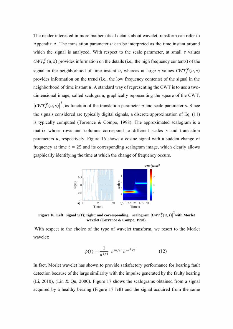
Figure 16. Left: Signal 𝐱(𝐭); right: and corresponding scalogram |𝑪𝑾𝑻𝒙𝝍(𝒖, 𝒔)|
𝟐with
Morlet wavelet (Torrence & Compo, 1998). .................................................................. 41
Figure 17. Left: scalogram of a signal acquired by a healthy bearing; Right: scalogram
of the signal acquired from the same bearing at the end of his life ................................ 42
Figure 18. Left: scalogram of a signal acquired by a healthy bearing before applying
Step 2; Right: scalogram of the signal acquired from the same bearing at the end of its
life before applying Step 2.............................................................................................. 44
Figure 19. Left: scalogram of a signal acquired by a healthy bearing after applying Step
2 with 𝒂𝒎𝒂𝒙 = 𝟏; Right: scalogram of the signal acquired from the same bearing at the
end of its life after applying Step 2 with 𝒂𝒎𝒂𝒙 = 𝟏. ...................................................... 45
Figure 20. Experimental test setup. ................................................................................ 48

List of Tables
Table 1. Validation set partition. .................................................................................... 31
Table 2. Test set partition. .............................................................................................. 31
Table 3. Comparison of the performance of the proposed method with the PCA based
approach.......................................................................................................................... 34
Table 4. Percentage of missed alarms considering sensor malfunctions of low, medium
and high intensities. ........................................................................................................ 34
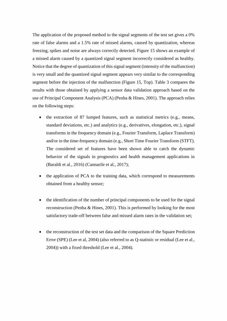
Table 5. Percentage of missed alarms considering multiple sensor malfunctions. ........ 35
Table 6. Description of the available bearing degradation trajectories. ......................... 49
Table 7. Data partitioning. .............................................................................................. 50
Table 8. Estimated hyperparameter set for each fold ..................................................... 50
Table 9. Estimated hyperparameter set for each fold ..................................................... 51
Table 10. Results ............................................................................................................ 51


Abstract
The detection of the onset of a degradation process and the identification of the
degradation level are fundamental tasks for the development of condition-based
maintenance approaches in industrial systems, which are expected to increase their
availability and safety, and, at the same time, reduce maintenance costs. The scope of the
present thesis work is the development of fault detection and diagnostic methods for
industrial systems. We consider the very common case in which, given the unavailability
of reliable physics-based models of the degradation process, data-driven methods should
be adopted. The detection and diagnostic models have typically to deal with non-
stationary time series, characterized by the fact that the frequency content of the signals
changes over time. This is due to the modifications of the environment in which the
industrial components operate and the effects of the degradation process on the measured
signals. The problem of properly treating these nonstationary time series for extracting
indicators of the equipment health state is also complicated by the presence of large noise
levels, which may mask the effects of the degradation. To tackle this issue, in this thesis
work, we propose a novel method which combines the use of Continuous Wavelet
Transform (CWT) with image analysis techniques. CWTs have been used due to their
ability to construct a time-frequency representation of a signal able to identify non-
stationary components with good time and frequency localization. The main steps of the
proposed method are: i) performing the CWT of the test signal, ii) building the
corresponding scalogram image and iii) comparing it with scalogram images obtained
from historical data collected from similar equipment in nominal conditions by means of
a properly defined similarity measure based on a pixel by pixel comparison. The
developed approach is applied with success to two experimental datasets concerning
sensor validation and bearing fault detection. The industrial problems of detecting
malfunctions of the sensors of an energy production plant and detecting anomalous
behaviors of the bearings of an engine.


Estratto
La detection del principio di deterioramento e l’identificazione della sua gravità sono dei
compiti fondamentali per lo sviluppo di approcci di manutenzione condition based i quali
mirano ad aumentare l'affidabilità e la sicurezza dell'intero sistema, e a ridurre i costi di
manutenzione. L’obiettivo di questa tesi è sviluppare un metodo di fault detection e
diagnostica per sistemi industriali. Consideriamo lo scenario comune nel quale, data
l’indisponibilità di modelli fisici affidabili per il processo di deterioramento, gli approcci
data-driver sono più efficaci. I modelli di detection e di diagnostica in genere devono
trattare time-series non stazionarie, cioè segnali la cui frequenza cambia nel tempo. Ciò
è dovuto alle modifiche dell’ambiente nel quale i componenti industriali operano e agli
effetti del processo di deterioramento sul segnale misurato. Il problema di trattare in
maniera adeguata time-series non stazionarie per estrarre indicatori sullo stato dei
componenti è anche complicato dalla presenza di rumore che può mascherare gli effetti
del deterioramento. Per affrontare il problema, in questa tesi, proponiamo un nuovo
metodo che unisce la Continuous Wavelet Transform (CWT) con l’analisi di immagine.
Le CWTs sono state già usate per la loro capacità di costruire una rappresentazione
tempo-frequenza di un segnale in grado di evidenziare le componenti non stazionarie. I
principali step del metodo sono: i) fare la CWT del segnale test, ii) ottenere la
corrispettiva immagine di scalogramma e iii) confrontarla con le immagini di
scalogrammi ottenute da dati storici di componenti simili in condizioni nominali mediante
una appropriata misura di similarità basata su un confronto pixel-pixel. Il metodo
sviluppato è stato applicato con successo a 2 dataset sperimentali, utilizzati
rispettivamente per la sensor data validation e la fault detection di cuscinetti.

1 Introduction
Prognostics and Health Management (PHM) is a field of research and application which
aims at making use of past, present and future information on the environmental,
operational and usage conditions of an equipment in order to achieve system reliability,
safety, maintainability, availability, supportability, and economic affordability (Zio,
2013). The main features of PHM include fault detection, isolation, degradation level
assessment, prognostics and maintenance decision (Pecht & Kang, 2010). In details,
prognostics predicts when (detection) and where (isolation) failure will occur letting the
users be able to mitigate system-level risks. The modern acquisition tools allow
continuously monitoring the equipment, recording in real-time signal values of the
physical parameters of interest (e.g., pressure, temperature, flow and vibration) (Jardine
et al, 2015), (Teng et al. 2016). In situations in which developing physics-based models
of the degradation and failure behavior of an equipment is not possible or favorable and
when sufficient historical data are available, data-driven PHM approach are typically
exploited (Schwabacher, 2005). Indeed, in contrast to model-based approaches which
require a priori knowledge of the process and equipment behavior, data-driven
approaches are developed on the basis of historical data (Hines & al, 2008). The acquired
signals are typically non-stationary, i.e., its frequency content changes over time, and
then, classical frequency analysis techniques based on Fourier Transform (FT) fail to
detect changes of the signal frequency content over time (Jaber & Bicker, 2014). In fact,
since FT does not provide any information about the time localization of important events,
it does not allow to properly detecting imminent faults or changes in the health state of
the component. For this reason, in this work will consider the development and
application of Time-Frequency methods (TF) which can reveal time variant features at
both high and low-frequency bands of nonstationary signal. The TF transform adopted in
this work is the Continuous Wavelet Transform (CWT). CWT is performed on the test
signal and a scalogram image is extracted. Following this, a pixel comparison is
performed between the extracted scalogram and scalograms which represent normal
operation of the monitored component and the test signal is then classified as anomalous
or non-anomalous. The practical industrial benefit of the technique is a visual
representation of fault detection.

In this work the proposed method is firstly applied to a real industrial case study
concerning the identification of anomalous signals recorded by a sensor, which we will
refer to sensor data validation. In fact, modern industrial plants are complex systems,
equipped with hundreds of sensors to measure physical parameters, such as pressures,
temperatures and flows for operation control and diagnostic purposes. In practice, sensors
may malfunction, i.e. they can provide inaccurate readings of the monitored physical
parameters. The most common types of sensor malfunctions are: freezing (or constant),
noise, spike (or short) quantization (Sharma et al., 2010) (Tolle et al., 2005). They can
lead to the incorrect intervention of plant operators and automatic control systems,
causing undesirable consequences, such as unnecessary component downtimes, or even
plant shutdowns with associated large financial losses. Thus, the task of promptly
detecting the occurrence of a sensor malfunction is of paramount importance. In particular
in our case the sensor data validation involves the following steps: 𝑖) performing the CWT
of the test signal,𝑖𝑖) computing the corresponding scalogram image and 𝑖𝑖𝑖) comparing
this scalogram with those obtained from historical data of the signals collected by the
sensor. With respect to the last step, the comparison between scalogram images is
performed by defining a proper measure of similarity between images based on a pixel
by pixel comparison. The same technique is then applied to the detection of the bearing
degradation onset through the analysis of its vibrational signal. Bearings in fact are the
most critical component in all rotating machineries and are the main cause of failure of
those machineries (Singleton et al. 2013). For this reason they are monitored through
several vibration sensors in order to acquire significant information about their health
state. We decided to apply the method also to the bearing degradation onset due to the
similarity with the sensor data validation task. In fact in both cases the signals are non-
stationary, due to the rapid changes of working conditions, in both cases the anomaly
alters the frequency content and in both cases a sufficient amount of historical data are
available to develop a data-driven model.
2 Sensor data validation
2.1 Introduction
Modern energy production plants are complex systems, equipped with hundreds of
sensors to measure, at relative high frequency, physical parameters, such as pressures,
temperatures and flows for operation control and diagnostic purposes. In practice, sensors
may malfunction, i.e. they can provide inaccurate readings of the monitored physical
parameters. The most common types of sensor malfunctions are: freezing (or constant),
noise, spike (or short) and quantization (Sharma et al., 2010) (Tolle et al., 2005). They
can lead to the incorrect intervention of plant operators and automatic control systems,
causing undesirable consequences, such as unnecessary component downtimes, or even
plant shutdowns with associated large financial losses. Thus, the task of promptly
detecting the occurrence of a sensor malfunction, which is often referred to as sensor data
validation, is of paramount importance. It has been addressed by a variety of methods
including Auto Associative Neural Network (AANN) (Wrest et al., 1996) (Hines et al.,
1998), Nonlinear Partial Least Squares Modeling (NLPLS) (Rasmussen et al., 2000),
Principal Component Analysis (PCA) (Penha & Hines, 2001) (Baraldi et al., 2011), Auto
Associative Kernel Regression (Baraldi et al., 2015) (Garvey et al., 2007), and
Multivariate State Estimation Technique (MSET) (Gross et al., 1997) (Zavaljevski &
Gross, 2000) (Coble et al., 2012).
A limitation of these approaches is that they only detect the abnormal behavior of the
measured signals, which, however, can be due to several causes, such as a sensor
malfunction, a process anomaly, a failure of a plant component. The subsequent
identification of the cause of the abnormal behavior is typically a time-consuming task,
which requires an intervention of the plant personnel or the use of other dedicated
diagnostic systems. Furthermore, data validation approaches typically detect the
anomalous behavior of a sensor using information provided by other sensors. The basic
idea is that a sensor malfunction causes a modification of the functional relationships
among the measured signal values. The use of data collected from other sensors may
cause difficulties from a practical point of view. For example, when hundreds of signals
are monitored in a plant, it is necessary to group them into several subsets, since it has
been shown in (Roverso et al., 2007), (Baraldi et al., 2011) that a single model based on

all (hundreds) signals is not able to provide satisfactory performances. Although the
problem of sensor grouping has been successfully addressed in (Baraldi et al., 2011) and
(Baraldi et al., 2014) by using ensemble of models dedicated to detection of sensor
malfunctions in a specific group of sensors, the proposed solutions have still some
practical limitations:
1. the necessity of periodically updating the models and the corresponding signal
grouping to take into account possible modifications of the signal relationships
(Roverso et al., 2007);
2. the fact that these models are not easily scalable to a fleet of plants (Baraldi et al.
2011). Since each plant has its own characteristics and, therefore, it requires a
dedicated grouping of the signals.
To overtake these limitations, we aim at developing a completely different approach for
detecting sensor malfunctions. The idea is to develop a dedicated data validation model
for each sensor, based on historical data collected from the sensor itself when it was
healthy. Since the approach does not consider relationships among different signals, it
can be systematically applied to a fleet of plants without requiring sensor grouping.
The proposed sensor data validation method builds up from the idea that a sensor fault
alters the regularity of a signal, i.e., its degree of smoothness. Continuous Wavelet
Transforms (CWT) are able to characterize and quantify the local regularity of a signal
(Mallat, 2008), and have been employed in many engineering applications. For example,
the Lipshitz-exponent, which can be estimated from CWT by using the Wavelet Modulus
Maxima (WMM) (Mallat & Hwang, 1992), has been used for bearing faults diagnostics
(Li, 2010), machinery health monitoring (Miao et al., 2007) and signal denoising (Mallat
& Hwang, 1992). A limitation of WMM is that it is sensible only to signal irregularities,
whereas it does not allow detecting types of sensor malfunctions which add regularity to
a signal, such as freezing. For this reason, in this work, we propose a novel method based
on the use of CWT scalograms, which are two-dimensional images representing the time
evolution of the squared magnitude (or power) of the CWT at different frequencies
(Mallat, 2008).
The method combines the use of CWT with image analysis techniques for the
identification of the similarity among the test data and an archive of historical data. It
involves the following steps:𝑖) performing the CWT of the test signal,𝑖𝑖) computing the

corresponding scalogram image and 𝑖𝑖𝑖) comparing this scalogram with those obtained
from historical data of the signals collected by the sensor. With respect to the last step,
the comparison between scalogram images is performed by defining a proper measure of
similarity between images based on a pixel by pixel comparison.
The main contributions of this work are:
• the use of CWT scalogram images to detect sensor malfunctions;
• the development of a method which allows the detection of a sensor malfunction
without using data measured by other sensors, is robust to different sensor
malfunction types and intensities and able to graphically motivate the reasons of
the detection through the use of scalograms.
• an original analysis about the characteristics of the scalograms of the signals
measured in case of different types of sensor malfunctions.
The performance of the proposed method has been verified with respect to data taken
from an energy production plant. Realistic examples of sensor malfunctions have been
artificially injected in the data streams and the proposed method has been compared with
a literature PCA-based approach from the point of view of the percentage of false and
missed alarms. The remainder of the chapter is organized as follows. Section 2.2 and 2.3
highlights the main issues associated to sensor data validation, provides a description of
the most common sensor malfunction types, introduce the problem statement and the
notation. In Section 2.4, some mathematical features of CWT at the basis of the proposed
method are discussed. Section 2.5 provides an in-depth discussion of the proposed
method. The case study and the application of the proposed method are shown in Section
2.6. Finally, Section 2.7 concludes the chapter.
2.2 Sensor data validation
The objective of this chapter is the development of a sensor data validation method for
online detecting sensor readings deviating from the ground truth values of the monitored
physical parameters. Signal deviations can be triggered by a single sensor fault or by the
failure of a node with attached several sensors, because of hardware failure or sensor
internal malfunction (e.g., losing the connection with the sensor board). According to

(Sharma et al., 2010), these types of malfunction are considered as non-functional faults
since they only impact the fidelity of the reported data. The different types of sensor
malfunctions are typically classified as (Ni et al., 2009) (Sharma et al., 2010):
• Spike (or short): a sharp change in the measured value between two successive
measurements. It produces a single isolated sensor reading with a value that is
significantly far from the signal ground truth (Figure 1).
• Noise: the variance of the sensor readings increases and the data becomes highly
uncorrelated with the true signal values (Figure 2).
• Freezing (or constant): the sensor reports a constant value for a large number of
successive samples. It may precede and/or follow an unexpected signal jump, with
readings that may fall outside the range of the measured phenomenon. Figures 3
and 4 show some examples of freezing without and with jump, respectively.
• Quantization: a reduction of the analogue-to-digital resolution conversion.
Quantization replaces signal ground truth values with their approximations into a
finite set of discrete levels. In practice, the sensor reading is characterized by
intervals with constant values followed by sharp changes (Figure 5).
Figure 1. Example of sensor spike. Left: ground truth signal values; right: corresponding readings
in case of sensor spike.
Figure 2. Example of sensor malfunction due to noise. Left: ground truth signal values; right:
corresponding readings in case with noise.

Figure 3. Example of sensor freezing. Left: ground truth signal values; right: corresponding
readings in case of sensor freezing.
Figure 4. Example of sensor freezing with jump. Left: ground truth signal value; right:
corresponding readings in case of sensor freezing with jump
Figure 5. Examples of sensor quantization. Left: ground truth signal value; right: corresponding
readings in case of sensor quantization.
2.3 Problem Statement and Notation
Let 𝑥(𝑡) be the measurement of a generic plant sensor at time 𝑡. The objective of the
present chapter is the development of a method for promptly detecting the occurrence of
sensor malfunctions. We assume:
i. to have available the historical measurements 𝑥(𝜏), 𝜏 < 𝑡, performed by the
sensor itself when it was healthy;

ii. the data in 𝑥(𝜏) are representative of all the plant operating conditions.
Although it is difficult to fully meet this latter assumption in real industrial applications,
we observe that real sensor data collected for long periods of time (e.g. years) typically
include a very large spectra of plant operating conditions, including the most common
plant anomalies which do not involve sensor malfunctions.
The detection of the sensor malfunction is based on the analysis of the measurements in
the time window 𝑥𝐿(𝑡) = {𝑥(𝑡 − 𝐿 + 1); 𝑥(𝑡)} made by the last 𝐿 collected
measurements, which will be also referred to as test pattern. The historical measurements
𝑥(𝜏) are organized into 𝑆 training vectors of length 𝐿 containing the measurements in the
time windows 𝑥𝐿,𝑗 = {𝑥𝑗(1 + (𝑗 − 1)Δ), 𝑥𝑗((𝑗 − 1)Δ + 𝐿)}with 𝑗 = 1,… , 𝑆 and 0 ≤ Δ <
𝐿. 𝐿 − Δ represents the overlapping between two consecutive time windows, i.e. the last
𝐿 − Δ measurements of the 𝑗 − 𝑡ℎ vector 𝑥𝐿,𝑗 coincide with the first 𝐿 − Δ measurements
of the vector 𝑥𝐿,𝑗+1.
2.4 Continuous Wavelet Transforms For Sensor malfunction Detection
Signal measurements in energy production plants may show transients and non-stationary
behaviors. Therefore, time or frequency-domain methods, which have been developed for
stationary signals, cannot be applied with success to the sensor data validation task. Due
to the time-varying frequency spectrum of the signals, suitable time–frequency
decomposition tools are needed for real-time signal data validation. Time–frequency
analysis can identify the signal frequency components and reveal their time-variant
features. Various time–frequency analysis methods have been proposed and applied to
fault detection, diagnostics and prognostics. Among these, short-time Fourier transform
(STFT), wavelet transforms (WT), Hilbert–Huang transform (HHT), and Wigner–Ville
distribution (WVD) are the most commonly used approaches.
Wavelet transform is a mathematical tool that converts a signal into a different form (Gao
& Yan, 2011). The objective of the conversion is twofold: i) to reveal signal
characteristics that are hidden in the time domain and ii) to provide a more succinct
representation of the original signal. A base wavelet function 𝜓(𝑡) is needed in order to
perform the wavelet transform. A wavelet is a small wave that has an oscillating wavelike
characteristic and has its energy concentrated in time. A wavelet is used as template for
analyzing time-varying or nonstationary signals by decomposing the signal into a 2D,
time-frequency domain representation (Gao & Yan, 2011) (Mallat, 2008). For any real
signal 𝑥(𝑡) ∈ 𝐿2(ℝ), the Continuous Wavelet Transform (CWT) with scale parameter
𝑠 > 0, translation parameter 𝑢 ∈ ℝ and wavelet function 𝜓(𝑡) is:
𝐶𝑊𝑇𝑥𝜓(𝑢, 𝑠) = ∫ 𝑥(𝑡)
1
√𝑠𝜓 (
𝑡 − 𝑢
𝑠) 𝑑𝑡
+∞
−∞
(1)
The reader interested in more mathematical details about wavelet transform can refer to
Appendix A.
The translation parameter 𝑢 can be interpreted as the time instant around which the signal
is analyzed. With respect to the scale parameter, at small 𝑠 values 𝐶𝑊𝑇𝑥𝜓(𝑢, 𝑠) provides
information on the details (i.e., the high frequency contents) of the signal in the
neighborhood of time instant 𝑢, whereas at large 𝑠 values 𝐶𝑊𝑇𝑥𝜓(𝑢, 𝑠) provides
information on the trend (i.e., the low frequency contents) of the signal in the
neighborhood of time instant 𝑢. A standard way of representing the CWT is to use a two-
dimensional image, called scalogram, graphically representing the square of the CWT,
|𝐶𝑊𝑇𝑥𝜓(𝑢, 𝑠)|
2, as function of the translation parameter 𝑢 and scale parameter 𝑠. Since
the signals considered are typically digital signals, a discrete approximation of Eq. (1) is
typically computed (Torrence & Compo, 1998). The approximated scalogram is a matrix
whose rows and columns correspond to different scales 𝑠 and translation parameters 𝑢,
respectively. Figure 6 shows a cosine signal with a sudden change of frequency at time
𝑡 = 25 and its corresponding scalogram image, which clearly allows graphically
identifying the time at which the change of frequency occurs.

Figure 6. Left: Signal 𝒙(𝒕); right: and corresponding scalogram |𝑪𝑾𝑻𝒙𝝍(𝒖, 𝒔)|
𝟐
As mentioned earlier, a sensor malfunction alters the regularity of a signal, i.e., its degree
of smoothness. For example: a sensor malfunction causing spikes adds irregularity to a
signal, being a spike an approximation of a Dirac distribution, which is not differentiable
(Mallat & Hwang, 1992); a sensor malfunction causing freezing of the sensor readings
adds regularity to the signal, since a constant signal is differentiable infinite times. A
measure of the local regularity of a signal is provided by the Lipshitz exponent 𝛼 (Mallat
& Hwang, 1992) which is introduced, from a mathematical point of view, in Appendix
B. Considering a function 𝑥(𝑡), it is possible to show that:
• If 𝑥(𝑡) is uniformely Lipschitz 𝛼 > 𝑛 in the neighborhood of 𝑡0, this implies that
𝑥(𝑡) is necessarily 𝑛 times continuously differentiable in this neighborhood
(Mallat, 2008);
• 𝛼 equal to 1 implies that 𝑥(𝑡) is a continuously and differentiable function at 𝑡0;
• 𝛼 ∈ (0,1) implies that the function 𝑥(𝑡) is continuous at 𝑡0 but the first derivative
of the function at that point is not continuous;
• 𝛼 equal to 0 implies that the function is discontinuous at 𝑡0 but bounded in the
neighborhood of 𝑡0.
In (Struzik, 2001), the estimation of the Lipschitz-exponent at a given point 𝑡0 has been
obtained through the use of the Wavelet Modulus Maxima (WMM). A WMM is defined
as any point (𝑢0, 𝑠0) such that |𝐶𝑊𝑇𝑡𝜓(𝑢, 𝑠0)| is a local maximum at 𝑢 = 𝑢0 and the
maxima line consists of the points that are local maxima. The approximated estimation
of 𝛼 is provided by:
𝛼 = 2
1𝑧−1
∑ 𝑙𝑜𝑔2(𝑠=𝑧−1𝑠=1
𝐶𝑊𝑇𝑥𝜓(𝑢,𝑠+1)
𝐶𝑊𝑇𝑥𝜓(𝑢,𝑠)
)
(2)
where 𝑧 is the length of the maxima line that propagates from coarse scales to fine scales.
This equation has been successfully applied in many engineering problems, like bearing
faults diagnostics (Li, 2010), machinery health monitoring problems (Miao et al., 2007)
and signal denoising (Mallat & Hwang, 1992). These works typically rely on the fact that
any irregularity can be detected by finding the translation parameter 𝑢 at which WMM
converge at fine scales (Mallat & Hwang, 1992). Notice, however, that methods for 𝛼
estimation based on WMM are only able to provide a rough approximation, since they
exploit only the information carried out by the first and last points of the maxima line
(Miao et al., 2007). A common problem of WMM-based techniques for the estimation of
𝛼 is that the limited resolution of a discrete signal implies that the scale 𝑠 cannot be
arbitrarily small, causing approximations which can lead to inaccurate Lipschitz exponent
estimation (Tu et al., 2005). Therefore, the use of WMM for sensor data validation is
applicable to detect only those types of sensor malfunctions adding irregularity to a signal,
such as spike and noise, whereas those adding regularity to a signal, such as freezing,
cannot be properly detected since none of the maxima lines converge to the 𝑢
corresponding to the freezing (Mallat & Hwang, 1992).
To overcome these limitations of the use of WMM for sensor data validation, in this work
we propose to directly work on scalogram images. This original approach is motivated
also by the possibility of taking full advantage of the redundancy provided by the CWT,
which allows avoiding loss of information (Kovačević & Chebira, 2007a) and has been
shown useful in many applications such as feature extraction (Sengüler, 2016).
With respect to the choice of the type of wavelet transform notice that different sensor
malfunctions influence the 𝐶𝑊𝑇 coefficients in specific and different scale ranges, as it
will be shown in Section 2.4.1 and Appendix B. For this reason, an efficient sensor
validation tool should be based on a wavelet transform able to provide an accurate scale
localization such Morlet wavelet:
𝜓(𝑡) =1
𝜋1/4 𝑒𝑖𝜋𝑓0𝑡 𝑒−𝑡
2/2 (3)
which has been shown to provide more accurate scale localization than other types of
wavelet transforms (Karacan & Olea, 2014).

2.4.1 Analysis of the scalogram characteristics in correspondence of different
types of sensor malfunction
In this Section, we discuss the characteristics of the scalograms of the signals measured
in case of different types of sensor malfunctions.
2.4.1.1 Spike
Figure 7 shows the scalograms obtained from a signal acquired by a healthy sensor (Figure 7a)
and the same signal to which a spike has been artificially injected at time 𝑡 = 50 (Figure 7b).
Figure 7. Top: scalogram of the signal of Figure 1(a) acquired by a healthy sensor; bottom:
scalogram of the signal of Figure 1(b) corresponding to the same signal with a spike at 𝒕 = 𝟓𝟎.
As expected, the main difference between the two scalogram images is observed in the
neighborhood of the time at which the spike has been injected and consists in the abrupt
increasing of the wavelet coefficients at small scales. This result is coherent with the fact
that, from a theoretical point of view, a spike can be seen as an approximation of a Dirac
distribution which is characterized by a Lipschitz exponent equal to -1 (Mallat & Hwang,
1992). Thus, the wavelet transform modulus maxima increase proportionally to 1𝑠 over a
large range of scales in the corresponding neighborhood (Mallat & Hwang, 1992). In
conclusion, a spike can be recognized for its large coefficients in the scalogram at small
scales.
2.4.1.2 Noise
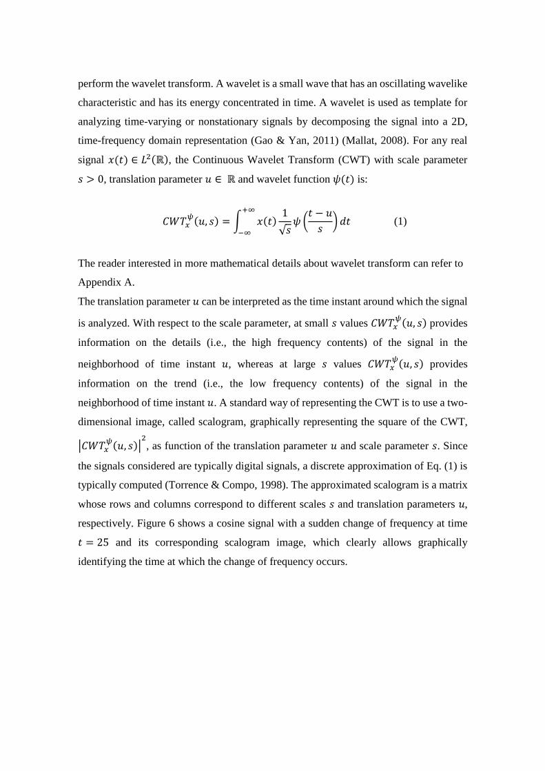
Figure 8 shows the scalograms obtained from a signal acquired by a healthy sensor
(Figure 8a) and the same signal to which noise has been artificially injected (Figure 8b).
The scalogram image shows larger CWT coefficients at all times in the case of presence
of noise. According to (Qiu et al., 2006), this is due to the fact that noise adds irregularity
to the signal in every sample, increasing its variance. In practice, a noisy signal shows
sharper changes than the nominal one, which can be seen as a combination of many low
intensity spikes. This implies CWT coefficients larger than in the case of a healthy sensor,
but smaller than those observed in correspondence of the spike.
Figure 8. Top: scalogram of the signal of Figure 2(a) acquired by a healthy sensor; bottom:
scalogram of the signal of Figure 2(b) corresponding to the same signal after artificially injecting a
noise malfunction.
2.4.1.3 Freezing
Figure 9 shows the scalograms obtained from a signal acquired by a healthy sensor
(Figure 3a) and the same signal to which a freezing has been artificially injected (Figure

3b). The scalogram obtained from the frozen signal is characterized by a large region with
zero CWT coefficients at small scale. The zero CWT coefficients are due to the fact that
when the wavelet atom 𝜓𝑢,𝑠(𝑡) support includes that of a constant signal 𝑥(𝑡) = 𝑐0, Eq.
(1) becomes:
𝐶𝑊𝑇𝑥𝜓(𝑢, 𝑠) = ∫ 𝑥(𝑡)
+∞
−∞
𝜓∗𝑢,𝑠(𝑡)𝑑𝑡 = ∫ 𝑐0𝜓
∗𝑢,𝑠(𝑡)𝑑𝑡
𝑠𝑢𝑝𝑝𝑜𝑟𝑡 𝜓𝑢,𝑠
= 0 (4)
where the last equality holds for the vanishing moment property (Eq. (33) in Appendix
B). Notice that, since the smaller is 𝑠, the smaller is the support of 𝜓𝑢,𝑠(𝑡), we can
conclude that for a fixed value of the translation parameter 𝑢, the support of the atom
𝜓𝑢,𝑎(𝑡) is included in that of the atom 𝜓𝑢,𝑏(𝑡) provided that 𝑎 < 𝑏. Thus, if the support
of 𝜓𝑢,𝑏(𝑡) includes the frozen signal interval, then also the support of 𝜓𝑢,𝑎(𝑡) includes
the same interval and, consequently, has a zero CWT coefficient. For this reason, the
region with zero CWT coefficient values becomes larger when 𝑠 decreases to zero and
tends to show a triangular shape (Figure 9).
Figure 9. Top: scalogram of the signal of the Figure 3(a) acquired by a healthy sensor; bottom:
scalogram of the signal of Figure 3(b) corresponding to the same signal after artificially injecting a
freeze without jump malfunction.
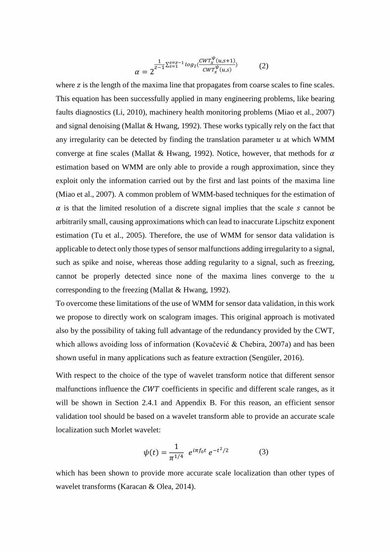
2.4.1.4 Quantization
Figure 10 shows the scalograms obtained from a signal acquired by a healthy sensor
(Figure 5a) and the same signal to which a quantization has been artificially injected

(Figure 5b). The comparison of these two Figures shows that the CWT coefficients at
large scales are very similar whereas there are differences at small scales. In detail, the
effect of the quantization is twofold:
• when the quantized signal is constant for several successive samples, the CWT
coefficients become smaller with respect to the same case without quantization
(dashed region in Figure 10b). This is due to the fact that the quantized signal
behaves like a frozen signal in this time interval;
• when quantization induces sudden jumps, the CWT coefficients become larger
than those of the same case without quantization. This is due to the fact that a
quantized signal behaves like a low intensity spike in these time intervals.
Thus, a quantized signal can be viewed as a signal in which short periods of freezing are
alternated to low intensity spikes.
Figure 10. Signal in nominal condition (left) corresponding to the same signal after artificially
injecting a quantization malfunction (right).
Figure 11. Top: scalogram of the signal of the Figure 5(a) acquired by a healthy sensor; bottom:
scalogram of the signal of Figure 5(b) corresponding to the same signal after artificially injecting a
quantization malfunction.
2.5 Sensor Malfunction Detection Method
The method proposed in this work is based on the idea of comparing the scalogram
obtained from the test vector 𝑥𝐿(𝑡) = {𝑥(𝑡 − 𝐿 + 1),… , 𝑥(𝑡)} to the scalograms obtained
from the training vectors 𝑥𝐿,𝑗 = {𝑥𝑗(1 + (𝑗 − Δ)), 𝑥𝑗((𝑗 − 1)Δ + 𝐿)}, 𝑗 = 1,… , 𝑆 , 0 ≤
Δ < 𝐿. First of all, each one of the training vector𝑥𝐿,𝑗 = 1,… 𝑆 is transformed in the
corresponding scalogram by applying the following procedure:
Step 1: Compute the CWT 𝐶𝑊𝑇𝑥𝐿𝝍 (𝑢, 𝑠) of the test vector 𝑥𝐿(t) and the corresponding
scalogram image 𝐼(𝑡). The scalogram 𝐼(𝑡) is a matrix of size 𝑁𝑥𝑀, where 𝑁 and 𝑀
depend on the discretization of the translation parameter 𝑢 (typically 𝑀 = 𝐿) and scale
parameter 𝑠. According to the results of the analysis of Section 2.4, large scale values do
not provide useful information for sensor malfunction detection and, consequently, the
analysis focuses on scale values lower than a prefixed threshold, i.e. 𝑠 < �̃�;
Step 2: Process the scalogram image to:

a) enhance the differences at low scales, which have been shown to be
relevant for the identification of a sensor malfunction caused by freezing
or quantization (Section 2.3.3 and 2.3.4);
b) normalize the intensities 𝐶𝑊𝑇𝑥𝐿𝝍 (𝑢, 𝑠) in the range [0, 1].
Step a) transforms the scalogram image 𝐼(𝑡) into a new scalogram image:
𝐼(𝑡)𝑝,𝑞 = {𝐼(𝑡)𝑝,𝑞𝑎𝑚𝑎𝑥
𝑖𝑓 𝐼(𝑡)𝑝,𝑞 ≤ 𝑎𝑚𝑎𝑥
𝑖𝑓 𝐼(𝑡)𝑝,𝑞 > 𝑎𝑚𝑎𝑥 (5)
where 𝑎𝑚𝑎𝑥 is a threshold. Step b) converts the scalogram 𝐼𝑗(𝑡) into a
greyscale image 𝐺𝑗(𝑡) by scaling its entries in the interval [0,1] as follows:
𝐺(𝑡)𝑝,𝑞 = 𝐼(𝑡)𝑝,𝑞 − 𝐼(𝑡)𝑚𝑖𝑛
𝐼(𝑡)𝑚𝑎𝑥 − 𝐼(𝑡)𝑚𝑖𝑛 (6)
where 𝐼(𝑡)𝑚𝑖𝑛 and 𝐼(𝑡)𝑚𝑎𝑥 are the minimum and the maximum values of the
matrix 𝐼(𝑡) in all the training scalograms.
Since two consecutive training vectors, 𝑥𝐿,𝑗 and 𝑥𝐿,𝑗+1,overlap of Δ − 𝐿 components
(Section 2.3), i.e., the last 𝐿 − Δ measurements of the 𝑗𝑡ℎ vector 𝑥𝐿,𝑗 coincides with the
first 𝐿 − Δ measurements of the vector 𝑥𝐿,𝑗+1, the effect on the scalogram of the
occurrence of an event, such as a plant transient, will be visible at different times in
different consecutive scalograms. This allows obtaining in the training scalograms an
overall representation of the signal measured by healthy sensors that is invariant from the
shift of the events.
Then, for the test vector 𝑥𝐿 , we repeat Steps 1 and 2 to obtain its corresponding scalogram
𝐼(𝑡). Notice that entries of matrix 𝐼(𝑡) (Eq. (5)) close to 𝑎𝑚𝑎𝑥 at low scales indicate sensor
malfunctions which add irregularity (i.e., noise and spike) and entries lower than 𝑎𝑚𝑎𝑥
indicate sensor malfunctions which add regularity (i.e., quantization and freezing). With
respect to matrix 𝐺(𝑡) in Eq. (6), entries close to 1 at low scales are typically of noise and
spike malfunctions, whereas entries close to 0 of quantization and freezing malfunctions.
Once the training and test grayscale images, 𝐺𝑗 and 𝐺, have been obtained, they are
compared by applying the following procedure:

a) Compute the dissimilarities 𝑑𝑗 between the greyscale image 𝐺(𝑡) and all the
greyscale images 𝐺𝑗 obtained from the historical signals 𝑥𝐿,𝑗, preprocessed
according to Steps 1-2:
𝑑𝑗 = ‖𝐺(𝑡) − 𝐺𝑗‖ 𝑗 = 1,… , 𝑆 (7)
where the matrix norm of the scalogram is:
‖𝐺(𝑡)‖ = ∑∑|𝐺(𝑡)𝑝,𝑞|
𝑀
𝑗=𝑞
𝑁
𝑝=1
(8)
b) Identify the scalogram of the training set most similar to the one currently tested,
i.e. the one characterized by the minimum dissimilarity 𝑑∗:
𝑑∗ = 𝑚𝑖𝑛𝑗=1,…,𝑆
𝑑𝑗 (9)
c) Compare 𝑑∗ with a fixed detection threshold 𝑇, if 𝑑∗ is greater than 𝑇, then a
sensor malfunction is detected.
Parameters 𝑇, 𝑎𝑚𝑎𝑥, and �̃� are set by minimizing a weighted sum of the number of false
and missed alarms, 𝑓𝑎 and 𝑚𝑎, on a validation set:
�̃� = 𝑤1𝑓𝑎 + 𝑤2𝑚𝑎 (10)
where the weights 𝑤1 and 𝑤2 are typically set by considering a proper trade off between
missed and false alarms. The validation set is formed by:
i. historical data collected when the sensor was healthy, different from those used
for the model training.
ii. Data representative of sensor malfunctions. If these latter data are not available,
they can be simulated using the procedure described in Appendix C.
Resorting to the big 𝑂 notation typically employed for evaluating algorithm complexity
(Wegener, 2005), the computational complexity of the different steps of the proposed
method is:
• step 1: 𝑂(𝑁𝐿 log 𝐿) for computing the wavelet transform of the test signal 𝑥𝐿(𝑡),
with 𝑂(𝐿 log 𝐿) representing the time complexity required per scale (Torrence &
Compo, 1998);

• step 2: 𝑂(𝑁𝐿) for scalogram preprocessing;
• step 3: 𝑂(𝑁𝐿𝑆) for computing all distances 𝑑𝑗;
• step 4: 𝑂(𝑆)
• step 5: 𝑂(1).
Notice that, in the worst case, i.e., when 𝐿 = 𝑁 = 𝑆, the computational complexity is
𝑂(𝐿3).
2.6 Case study
We consider a dataset containing real temperature measurements recorded at a sampling
frequency 𝑓𝑠 = 1 𝐻𝑧 from a component of an electricity production plant (Baraldi et al,
2015). The temperature signal has been segmented using a fixed time window of length
𝐿 = 120 samples (corresponding to 120 seconds), with overlapping of 20 samples. The
overlapping of the training pattern has been introduced to deal with the fact that a
malfunction can occur at any time of the test window. Therefore, in order to detect it,
various shifted training vectors with an overlap of 𝐿 − Δ = 20 samples are considered
in the training set. Since the available data have been collected by a healthy sensor, we
have artificially simulated sensor malfunctions of different types and intensities,
according to the procedure proposed in (Sharma et al., 2010) and reported in Appendix
C. We also assume that the historical signal vectors 𝑥𝐿,𝑗 collected from the same sensor
in healthy condition are representative of all the plant operational conditions. Figure 12
shows an example of signal behavior and Figure 13 examples of simulated low-intensity
sensor malfunctions.
Figure 12. Signal measurements obtained from a healthy sensor.

Figure 13. Simulated sensor malfunctions: freezing (top-left), spike (top-right), noise (down-left),
quantization (down-right).
2.6.1 Dataset partitioning
We have partitioned the available data into three subsets: 𝑖) a training set, 𝑖𝑖) a validation
set, and 𝑖𝑖𝑖) a test set. The training set is formed by 67 signal segments measured from a
healthy sensor and constitutes the set of vectors 𝑥𝐿,𝑗 from which the dissimilarity of the
test segment is computed in Step 3 (Section 2.5). The validation and test sets are formed
by 400 and 460 signal segments, respectively, and contain measurements from the healthy
sensor and artificially injected sensor malfunctions of different types and intensities,
according to the proportions of Tables 1 and 2. The validation set has been used to
determine the values of the parameters of the method: wavelet coefficient threshold 𝑎𝑚𝑎𝑥
(Step 2a), maximum scale �̃� (Step 1) and detection threshold 𝑇 (Step 5), whereas the test
set has been used to evaluate the performance of the proposed methodology. To better
mimic a real application, the signal segments of the training set temporally preceed those
of the validation set, which preceed those of the test set.

Type of sensor
malfunction
Number of signals in the
validation set
Freezing 100
Spike 100
Noise 100
Quantization 50
Healthy 50
Table 1. Validation set partition.
Sensor
malfunctions
Number of signals in the test
set
Freeze 100
Spike 100
Noise 100
Quantization 80
Healthy 80
Table 2. Test set partition.
2.6.2 Results
Wavelet coefficient threshold 𝑎𝑚𝑎𝑥, scale �̃� and detection threshold 𝑇 have been set by
minimizing the function �̃� Eq. (10) assuming 𝑤1 = 𝑤2 = 1, i.e., by giving same
importance to the contributes. By setting 𝑎𝑚𝑎𝑥 = 0.06, �̃� = 2.8, and 𝑇 = 884, we have
obtained the optimal trade off 1% of missed alarms and 4% of false alarms in the
validation set. This choice of the scale parameter �̃� results in a reduction of the original
scalogram dimensions from 591x120 to 50x120 with evident benefits in terms of
computational burden. Figure 14 shows the variations of the false alarm rates and of
different types of missed alarm rate with respect to variation of the detection threshold 𝑇.
It is interesting to observe that if the threshold 𝑇 is progressively increased, the first types
of missed alarms that occur are those caused by quantization and freezing malfunctions,
whereas spike and noise malfunctions are correctly recognized. This is due to the fact that
the scalograms corresponding to quantization and freezing malfunctions are more similar
to those obtained from a healthy sensor than those corresponding to spike and noise
malfunctions, as shown in Figures 7, 8, 9 and 11. Thus, the identification of quantization

and freezing malfunctions is more sensible to the threshold value than that of the spike
and noise malfunctions.
Figure 14. Variations of the false alarm rate (cross-dotted black line) and of the missed alarm rates
due to freezing (dashed blue curve), quantization malfunctions (dotted red curve), spike
malfunctions (circle-dotted purple curve), noise malfunctions (continuous green curve). The total
variation of the missed alarm rate is referred using the (dash-dot grey curve).
Figure 15. Example of missed alarm: the quantized signal segment (Top) and the corresponding
signal segment before the malfunction injection (Down).
The application of the proposed method to the signal segments of the test set gives a 0%
rate of false alarms and a 1.5% rate of missed alarms, caused by quantization, whereas
freezing, spikes and noise are always correctly detected. Figure 15 shows an example of
a missed alarm caused by a quantized signal segment incorrectly considered as healthy.
Notice that the degree of quantization of this signal segment (intensity of the malfunction)
is very small and the quantized signal segment appears very similar to the corresponding
segment before the injection of the malfunction (Figure 15, Top). Table 3 compares the
results with those obtained by applying a sensor data validation approach based on the
use of Principal Component Analysis (PCA) (Penha & Hines, 2001). The approach relies
on the following steps:
• the extraction of 87 lumped features, such as statistical metrics (e.g., means,
standard deviations, etc.) and analytics (e.g., derivatives, elongation, etc.), signal
transforms in the frequency domain (e.g., Fourier Transform, Laplace Transform)
and/or in the time-frequency domain (e.g., Short Time Fourier Transform (STFT).
The considered set of features have been shown able to catch the dynamic
behavior of the signals in prognostics and health management applications in
(Baraldi et al., 2016) (Cannarile et al., 2017);
• the application of PCA to the training data, which correspond to measurements
obtained from a healthy sensor;
• the identification of the number of principal components to be used for the signal
reconstruction (Penha & Hines, 2001). This is performed by looking for the most
satisfactory trade-off between false and missed alarm rates in the validation set;
• the reconstruction of the test set data and the comparison of the Square Prediction
Error (SPE) (Lee et al, 2004) (also referred to as Q-statistic or residual (Lee et al.,
2004)) with a fixed threshold (Lee et al., 2004).

METHOD
Percentage
of Missed
Alarm
Percentage of
False Alarm
Proposed Method 0% 1.25%
PCA-based Method
(𝑃 = 90%) 10.8%
1.25%
Table 3. Comparison of the performance of the proposed method with the PCA based approach.
The PCA proposed approach is less accurate than the proposed method: the percentage
of missed alarms increases from 0% to 10.8% (Table 3), with the same percentage of false
alarms.
We have evaluated the robustness of the proposed method with respect to different
intensities of the malfunctions, simulated according to (Sharma et al., 2010) (see
Appendix C). Table 4 reports the results in term of missed alarms for the different types
of sensor malfunctions. We can conclude that the method provides satisfactory
performances and, as expected, the overall percentage of missed alarms decreases as the
malfunction intensity increases.
Sensor
malfunctions
Low
Intensity
Medium
intensity
High
intensity
Freezing 0% 1% 0%
Spike 0% 0% 0%
Noise 0% 0% 0%
Quantization 6% 2% 0%
Table 4. Percentage of missed alarms considering sensor malfunctions of low, medium and high
intensities.
Furthermore, we have tested the proposed method on 100 signal segments characterized
by the simultaneous presence of two sensor malfunctions, obtained by randomly sampling
their times of occurrence and their intensities from the same probability distributions used
for the sampling low intensity single sensor malfunctions. Table 5 reports the results in
term of missed alarms for the different combinations of two sensor malfunctions. It is
interesting to observe that the percentage of missed alarms in case of quantization
malfunction decreases to 0% (it was 6% in case of single low intensity malfunction). This
is due to the fact that scalogram modifications caused by spike or noise malfunctions
(Figures 7 and 8) are easier to detect than those due to the quantization anomaly (Figure
11), and, therefore, the detection of the quantization malfunction is facilitated by the
simultaneous presence of spike and noise malfunctions
Sensor malfunctions Number of
segments
Missed
alarms
Quantization+Spike 20 0%
Quantization+Noise 20 0%
Freezing+Spike 20 0%
Noise+Spike 20 0%
Noise+Freeze 20 0%
Table 5. Percentage of missed alarms considering multiple sensor malfunctions.
With respect to the computational time, testing a signal segments formed by 𝐿 = 120
samples requires on average 0.052 seconds using an Intel Core i5-M430 @ 2.26 GHz
processor with 4 Gb RAM in a MATLAB 2017b environment. Therefore, the proposed
approach is suitable for being used in field operation.
2.7 Chapter conclusions
In this chapter, we have developed a novel method for sensor data validation, which
combines the use of Continuous Wavelet Transform with an image analysis technique.
Fault detection is performed by comparing the CWT scalogram obtained from the test
signal with those obtained from historical data of the same signal. The performance of
the method, measured in terms of false and missed alarm rates, is shown superior to that
of a PCA-based approach for data validation. From a practical point of view, the method,
differently from the traditional sensor data validation approaches which consider the

correlations among plant signals, is easily applicable to all the sensors of a fleet of plants
being the validation of the data measured from a sensor independent to that of other
sensors. Furthermore, it has been shown that the analysis of the obtained scalograms
allows distinguishing among the different types of sensor malfunction.
In this chapter, we have not considered the possible influence of one sensor malfunction
on the other sensor readings. In industrial complex systems characterized by many
interconnected components and in which the readings of some sensors are used for system
control, it can happen that one sensor malfunction causes anomalous behaviors in other
signals. In this case, although the proposed method correctly identifies the sensor affected
by the malfunction, it will also detect malfunctions in other sensors, which are correctly
working, but whose measured signals have anomalous behaviors due to the consequences
of the sensor malfunction.


3 Bearing degradation onset detection
3.1 Introduction
According to both the IEEE large machine survey and the Norwegian offshore and
petrochemical machines data, bearing-related defects are responsible of more than 40%
of the failure in industrial machines.Then, in industrial practice it is of great interest to
promptly detect the bearing degradation onset. At the earliest stage of bearing
degradation, information on the bearing health state, and, eventually, on the type of
degradation can be obtained by observing the machine vibrational behavior. In fact,
vibrations are among the most widely used signals for the detection of faults in the bearing
due to the defects in the inner race, outer race, or ball because these signals are an
indicator for bearing defects, provided that a suitable processing procedure is applied
(Bellini et al., 2008). Many studies have used vibration signals for bearing fault detection
(Li et al., 2000), (Amar et al., 2000) (Yang & Tang, 2011). In general approaches to fault
detection in bearings have been developed considering the vibrational signals in the
frequency domain and in time-frequency domain. In frequency-domain approaches, the
principal frequencies of the vibrational signals and their amplitudes are identified (Chebil
et al., 2009), (Blodt et al., 2008). Most of the proposed approaches to fault detection for
bearings in the frequency domain assume a priori knowledge of the principal frequencies
associated to the bearings faults (Chebil et al., 2009), moreover frequency-domain
method cannot localize the transients efficiently in time (Amar et al., 2015). This setting
is not feasible in many real cases where the environmental and operational conditions
modify the frequency spectra of the vibrational signals. Therefore, frequency-domain
methods, which have been developed for stationary signals, cannot be applied with
success to the bearing fault detection task. Due to the time-varying frequency spectrum
of the signals, suitable time–frequency decomposition tools are needed for real-time
bearing fault detection. Time–frequency analysis can identify the signal frequency
components and reveal their time-variant features. Various time–frequency analysis
methods have been proposed and applied to fault detection, diagnostics and prognostics.
Among these, short-time Fourier transform (STFT), Wavelet Transforms (WT), Hilbert–
Huang transform (HHT), and Wigner–Ville distribution (WVD) are the most commonly
used approaches. In (Gao et al., 2015) the STFT combined with non-negative matrix
factorization is used to detect the bearing fault from its vibrational signal. However,
accuracy of STFT might be a problem since constant-size windows are used in the
analysis for all frequencies. A better accuracy may be obtained by reducing the window
size, but inevitably increasing the computational burden (Jacop et al., 2017), moreover,
the detection of incipient faults, in which measured signals are weak, nonstationary and
masked with noises, requires a more flexible and effective approach (Jacop et al., 2017).
Wavelet transform seems to be a promising approach to overcome the window-size
problem as it provides a flexible window size for different frequencies (Jacod et al., 2017).
This characteristic makes it possible to analyze the vibration signals and detect better the
frequencies of the time-frequency varying signals. In (Li, 2010) an approach for detecting
localized faults in the outer or the inner races of a rolling element bearing based on CWT
is used. In (Jiang et al., 2014) an optimal lifting multiwavelet denoising method is
developed for bearing fault detection. In (Zhao et al., 2013) in order to track the
degradation trend of bearings a Morlet wavelet transform-based extraction method of is
proposed. In (Boufenar & Rechak, 2013) Sparse Code Shrinkage (SCS) method based on
maximum likelihood estimation for thresholding using an adapted wavelet is developed
for bearing fault detection. In this work, we propose a novel method for bearing fault
detection which combines the use of CWT with image analysis techniques for the
identification of the similarity among the test data and an archive of historical vibrational
data of healthy bearings. The CWT on the other hand uses a set of non-orthogonal wavelet
frames to provide highly redundant information that is suitable for detection of various
types of faults (Kovačević & Chebira, 2007 a). CWT is easier to interpret since its
redundancy tends to reinforce the relevant features for fault detection (Kovačević &
Chebira, 2007 b) and gains in “readability” and in representation, what it losses in terms
of computational burden, which is surely an important problem to be accounted but of
secondary importance when suitable feature extraction is the main objective.
For these reasons, we resort to the CWT coupled with image analysis, in fact in this way
all the information contained in the CWT are properly exploited and image processing
gives the possibility to visualize and efficiently refine the spectral features by eliminating

insignificant frequencies of incoherent noise, distributed over the entire spectral image
using a threshold technique (Amar et al., 2012).
In details, our method involves the following steps:𝑖) performing the CWT of the test
signal,𝑖𝑖) computing the corresponding scalogram image and 𝑖𝑖𝑖) comparing this
scalogram with those obtained from historical data of the vibrational signals collected by
healthy bearings. With respect to the last step, the comparison between scalogram images
is performed by defining a proper measure of similarity between images based on a pixel
by pixel comparison.
The performance of the proposed method has been verified with respect to data generated
by the NSF I/UCR Center for Intelligent Maintenance Systems (Qiu et al., 2006).
The remainder of the paper is organized as follows. In Section 3.2, some mathematical
features of CWT at the basis of the proposed method are discussed. Section 3.3 provides
the problem assumptions. Section 3.4 provides an in-depth discussion of the proposed
method. The case study and the application of the proposed method are shown in Section
3.5. Finally, Section 3.6 concludes the chapter.
3.2 Continuous Wavelet Transform for Bearing Fault Detection
Continuous Wavelet transform is a mathematical tool that converts a signal into a
different form (Gao & Yan, 2011). The objective of the conversion is twofold: i) to reveal
signal characteristics that are hidden in the time domain and ii) to provide a more succinct
representation of the original signal. A base wavelet function 𝜓(𝑡) is needed in order to
realize the wavelet transform. The wavelet is a small wave that has an oscillating wavelike
characteristic and has its energy concentrated in time. A wavelet is used as template for
analyzing time-varying or nonstationary signals by decomposing the signal into a 2D,
time-frequency domain (Gao & Yan, 2011) (Mallat, 2008). For any real signal 𝑥(𝑡) ∈
𝐿2(ℝ), the Continuous Wavelet Transform (CWT) with scale parameter 𝑠 > 0,
translation parameter 𝑢 ∈ ℝ and wavelet function 𝜓(𝑡) is:
𝐶𝑊𝑇𝑥𝜓(𝑢, 𝑠) = ∫ 𝑥(𝑡)
1
√𝑠𝜓 (
𝑡 − 𝑢
𝑠) 𝑑𝑡
+∞
−∞
(11)
The reader interested in more mathematical details about wavelet transform can refer to
Appendix A. The translation parameter 𝑢 can be interpreted as the time instant around
which the signal is analyzed. With respect to the scale parameter, at small 𝑠 values
𝐶𝑊𝑇𝑥𝜓(𝑢, 𝑠) provides information on the details (i.e., the high frequency contents) of the
signal in the neighborhood of time instant 𝑢, whereas at large 𝑠 values 𝐶𝑊𝑇𝑥𝜓(𝑢, 𝑠)
provides information on the trend (i.e., the low frequency contents) of the signal in the
neighborhood of time instant 𝑢. A standard way of representing the CWT is to use a two-
dimensional image, called scalogram, graphically representing the square of the CWT,
|𝐶𝑊𝑇𝑥𝜓(𝑢, 𝑠)|
2, as function of the translation parameter 𝑢 and scale parameter 𝑠. Since
the signals considered are typically digital signals, a discrete approximation of Eq. (11)
is typically computed (Torrence & Compo, 1998). The approximated scalogram is a
matrix whose rows and columns correspond to different scales 𝑠 and translation
parameters 𝑢, respectively. Figure 16 shows a cosine signal with a sudden change of
frequency at time 𝑡 = 25 and its corresponding scalogram image, which clearly allows
graphically identifying the time at which the change of frequency occurs.
Figure 16. Left: Signal 𝒙(𝒕); right: and corresponding scalogram |𝑪𝑾𝑻𝒙𝝍(𝒖, 𝒔)|
𝟐with Morlet
wavelet (Torrence & Compo, 1998).
With respect to the choice of the type of wavelet transform, we resort to the Morlet
wavelet:
𝜓(𝑡) =1
𝜋1/4 𝑒𝑖𝜋𝑓0𝑡 𝑒−𝑡
2/2 (12)
In fact, Morlet wavelet has shown to provide satisfactory performance for bearing fault
detection because of the large similarity with the impulse generated by the faulty bearing
(Li, 2010), (Lin & Qu, 2000). Figure 17 shows the scalograms obtained from a signal
acquired by a healthy bearing (Figure 17 left) and the signal acquired from the same

bearing at the end of his life (Figure 17 right) when it was faulty. Both signals have been
recorded at sampling frequency 𝑓𝑠=20000 𝐻𝑧.
Figure 17. Left: scalogram of a signal acquired by a healthy bearing; Right: scalogram of the signal
acquired from the same bearing at the end of his life
The main differences between the two scalogram images in Figure 17 is observed at small
scale, in particular at scales 100-200 corresponding to frequencies between 4-8kHz. The
increase of energy density at these frequencies is due to higher harmonics of the
characteristic frequency of the signal related to a defect on the bearing (Jacop et al., 2017).
3.3 Problem Statement and Notation
Let 𝑥(𝑡) be the measurement of the bearing vibration signal at time 𝑡. The objective of
the present work is to develop a method for promptly detecting the onset of the bearing
degradation. We assume that the historical measurements 𝑥(𝜏), 𝜏 < 𝑡, are available, taken
by the bearing itself when it was healthy (at the beginning of its life). The detection of the
bearing degradation onset is based on the analysis of the last 𝐿 measurements collected in
the time window 𝑥𝐿(𝑡) = {𝑥(𝑡 − 𝐿 + 1),… , 𝑥(𝑡)}, which will be also referred to as test
pattern. The historical measurements 𝑥(𝜏) are organized into 𝑆 vectors of length 𝐿
containing the measurements in the time windows 𝑥𝐿,𝑗 = {𝑥𝑗(1 + (𝑗 − 1)𝐿), 𝑗𝐿)} with
𝑗 = 1,… , 𝑆 and will be referred to as training-set. In addition, we also assume to have
available historical degradation trajectories from 𝑄 bearings similar to the one currently
monitored. Among the available 𝑄 degradation trajectories 𝑄𝐹 < 𝑄 are run-to-failure
degradation trajectories for which an onset of degradation has been detected and the
remaining 𝑄𝐻 = 𝑄 − 𝑄𝐹 are right-censored degradation trajectories for which no onset
of degradation has been detected. We will refer to these 𝑄 degradation trajectories as
validation-set. The measurement collected from the 𝑞𝑡ℎ, 𝑞 = 1,… , 𝑄𝐹 , 𝑄𝐹 + 1,… , 𝑄,
bearing in the validation set are organized into 𝐵𝑞 vectors of length 𝐿 containing the
measurements in the time windows 𝑥𝐿,𝑗𝑞,𝑞 = {𝑥𝑗
𝑞(1 + (𝑗𝑞 − 1)𝐿), 𝑗𝑞𝐿)} with 𝑗𝑞 =
1,… , 𝐵𝑞. The time windows of a faulty bearing corresponding to the onset of the
degradation will be indexed as 𝑡𝑞. For the 𝑄𝐹 faulty bearings the 𝐵𝑞 time windows are
further divided into two subsets 𝑆𝐻𝑞 and 𝑆𝐹
𝑞 containing the first 𝑡𝑞 − 1 time windows and
the remaining 𝐵𝑞 − 𝑡𝑞 + 1 time windows, respectively, i.e., 𝑆𝐻𝑞 contains time-windows
before the onset of the degradation and 𝑆𝐹𝑞 those after the onset of the degradation.
3.4 Bearing Fault Detection Method
The method proposed in this work is based on the idea of comparing the scalogram
obtained from the test vector 𝑥𝐿(𝑡) = {𝑥(𝑡 − 𝐿 + 1),… , 𝑥(𝑡)}, a signal segment, to the
scalograms obtained from the training vectors 𝑥𝐿,𝑗 = {𝑥𝑗(1 + (𝑗 − 1)L), 𝑥𝑗(𝑗𝐿)}, 𝑗 =
1, … , 𝑆.
First of all, each one of the training vector 𝑥𝐿,𝑗, = 1,… , 𝑆, is transformed in the
corresponding scalogram by applying the following procedure:
Step 1: Compute the Continuous Wavelet Transform (CWT) 𝐶𝑊𝑇𝑥𝐿𝝍 (𝑢, 𝑠) of the test
vector 𝑥𝐿(𝑡) and the corresponding scalogram image 𝐼(𝑡). The scalogram 𝐼(𝑡) is a matrix
of size 𝑁𝑥𝑀, where 𝑁 and 𝑀 depend on the discretization of the translation parameter 𝑢
and scales parameters. We will focus our analysis only on scale values lower than a
prefixed threshold, i.e. 𝑠 < �̃�. �̃� is an algorithm parameter that impact the number of rows
considered in the matrix 𝐼(𝑡). Considering only scale values 𝑠 < �̃� means considering
only the first �̃� rows of the matrix 𝐼(𝑡). Our algorithm parameter from now will be the
numbers of rows �̃� considered in the matric 𝐼(𝑡) instead of �̃�
Step 2: Process the scalogram image to:
a) enhance the differences between the scalogram of signals from a healthy bearing and
the scalogram of signals from a faulty bearing
b) normalize the intensities 𝐶𝑊𝑇𝑥𝐿,𝑗𝝍 (𝑢, 𝑠) in the range [0, 1].
Step a) transforms the scalogram image 𝐼(𝑡) into a new scalogram image:

𝐼𝑗(𝑡)𝑝,𝑞 = {𝐼𝑗(𝑡)𝑝,𝑞𝑎𝑚𝑎𝑥
𝑖𝑓 𝐼𝑗(𝑡)𝑝,𝑞 ≤ 𝑎𝑚𝑎𝑥
𝑖𝑓 𝐼𝑗(𝑡)𝑝,𝑞 > 𝑎𝑚𝑎𝑥 (13)
where 𝑎𝑚𝑎𝑥 is a threshold.
Step b) converts the scalogram 𝐼𝑗(𝑡) into a greyscale image 𝐺𝑗(𝑡) by scaling its
entries in the interval [0,1] as follows:
𝐺𝑗(𝑡)𝑝,𝑞 = 𝐼𝑗(𝑡)𝑝,𝑞 − 𝐼
𝑗(𝑡)𝑚𝑖𝑛
𝐼𝑗(𝑡)𝑚𝑎𝑥 − 𝐼𝑗(𝑡)𝑚𝑖𝑛 (14)
where 𝐼𝑗(𝑡)𝑚𝑖𝑛 and 𝐼𝑗(𝑡)𝑚𝑎𝑥 are the minimum and the maximum values of the
matrix 𝐼𝑗(𝑡) in all the training scalograms.
Then, for the test vector 𝑥𝐿 , we repeat Steps 1 and 2 to obtain its corresponding scalogram
𝐼(𝑡).
Figure 18 shows the scalograms obtained before applying Step 2 from vibration signals
corresponding to the bearing in healthy condition (Figure 18 left) and the vibration signal
acquired from the same bearing at the end of its life (failure) (Figure 18 right). Figure 19
shows the same scalograms shown in Figure 18 after the application of Step 2.
Figure 18. Left: scalogram of a signal acquired by a healthy bearing before applying Step 2; Right:
scalogram of the signal acquired from the same bearing at the end of its life before applying Step 2.
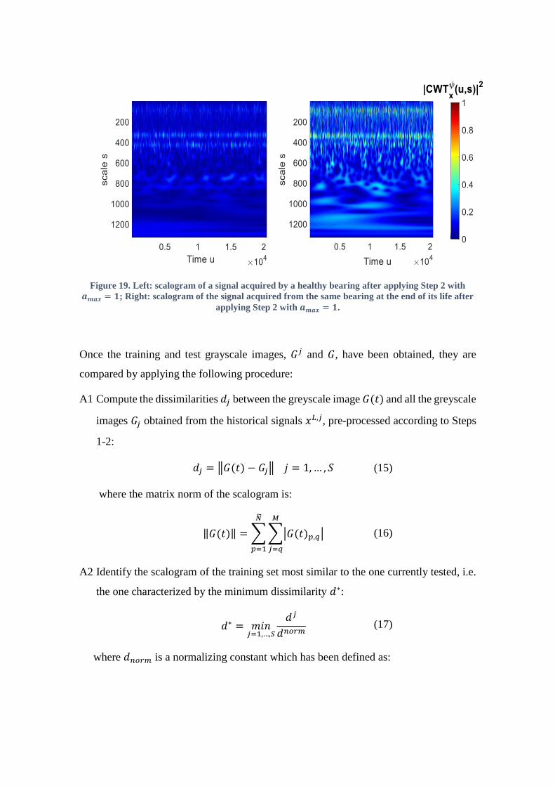
Figure 19. Left: scalogram of a signal acquired by a healthy bearing after applying Step 2 with
𝒂𝒎𝒂𝒙 = 𝟏; Right: scalogram of the signal acquired from the same bearing at the end of its life after
applying Step 2 with 𝒂𝒎𝒂𝒙 = 𝟏.
Once the training and test grayscale images, 𝐺𝑗 and 𝐺, have been obtained, they are
compared by applying the following procedure:
A1 Compute the dissimilarities 𝑑𝑗 between the greyscale image 𝐺(𝑡) and all the greyscale
images 𝐺𝑗 obtained from the historical signals 𝑥𝐿,𝑗, pre-processed according to Steps
1-2:
𝑑𝑗 = ‖𝐺(𝑡) − 𝐺𝑗‖ 𝑗 = 1,… , 𝑆 (15)
where the matrix norm of the scalogram is:
‖𝐺(𝑡)‖ = ∑∑|𝐺(𝑡)𝑝,𝑞|
𝑀
𝑗=𝑞
�̃�
𝑝=1
(16)
A2 Identify the scalogram of the training set most similar to the one currently tested, i.e.
the one characterized by the minimum dissimilarity 𝑑∗:
𝑑∗ = 𝑚𝑖𝑛𝑗=1,…,𝑆
𝑑𝑗
𝑑𝑛𝑜𝑟𝑚 (17)
where 𝑑𝑛𝑜𝑟𝑚 is a normalizing constant which has been defined as:
𝑑𝑛𝑜𝑟𝑚 = (∑ (𝑑𝑗
∗)2𝑆𝑧=1
𝑆)
0.5
(18)
𝑑𝑗∗ = 𝑚𝑖𝑛
𝑗=1,…,𝑆\{𝑘}𝑑𝑗,𝑘
(19)
In Eq. (19) 𝑑𝑗,𝑘 represents the dissimilarity between the scalogram of the 𝑗𝑡ℎ vibrational
signal in the training set with the scalogram of the 𝑘𝑡ℎ vibrational signal in the training
set, with 𝑗 ≠ 𝑘. Finally, the value 𝑑∗ is compared with a fixed detection threshold 𝑇∗: if
𝑑∗ is greater than 𝑇∗ for 𝑁∗ consecutive test vector then a degradation onset is detected.
The reason behind the decision to detect an alarm only if 𝑑∗ is greater than 𝑇∗ for 𝑁∗ is
to isolate the real degradation onset, an irreversible alteration that last for all the remaining
bearing life, from other temporary perturbations; the latter in fact will influence some
consecutive test signals but they won’t give an alarm if a proper 𝑁∗ is set.
In details, 𝑎𝑚𝑎𝑥, and �̃� are set by maximizing the dissimilarities among the scalograms of
the time-windows of the 𝑄𝐹 before the degradation onset with those after the degradation
onset. To do so, given a candidate threshold �̇� and a candidate number of rows �̇�, for each
of the 𝑄𝐹 faulty bearings we divide 𝑆𝐻𝑞 into two subsets 𝑇𝐻
𝑞 and 𝐻𝐻
𝑞. 𝑇𝐻
𝑞 contains the first
𝑟𝑞 time windows in 𝑆𝐻𝑞 and 𝐻𝐻
𝑞 contains the remaining 𝑡𝑞 − 1 − 𝑟𝑞 time-windows. For
each 𝑞 bearing of the 𝑄𝐹 faulty bearings we transform, doing the step 1 and 2 of the
method in Section 3.4 with threshold �̇� and number of rows �̇�, all the time-windows in
𝑇𝐻𝑞. Then we define 𝑑𝑞,𝑝
𝑗,𝐹 the distance in Eq. (15) between the scalogram of the signal
segment 𝑝 in 𝑆𝐹𝑄
and the scalogram of the signal segment 𝑗 in 𝑇𝐻𝑞, processed as step 1 and
2 of the method in Section 3.4 with threshold �̇� and number of rows �̇�, and finally the
distance 𝑑𝑞,𝑝∗,𝐹
is defined as:
𝑑𝑞,𝑝∗,𝐹 = 𝑚𝑖𝑛
𝑗=1,…,𝑟𝑞𝑑𝑞,𝑝𝑗,𝐹
(20)
In the same way, defining 𝑑𝑞,𝑝𝑗,𝐻
the distance in Eq. (15) between the scalogram of the
signal segment 𝑝 in 𝐻𝐹𝑄
and the scalogram of the signal segment 𝑗 in 𝑇𝐻𝑞, processed as
step 1 and 2 of the method in Section 3.4 with threshold �̇� and number of rows �̇�, then the
distance 𝑑𝑞,𝑝∗,𝐻
is defined as:
𝑑𝑞,𝑝∗,𝐻 = 𝑚𝑖𝑛
𝑗=1,…,𝑟𝑞𝑑𝑞,𝑝𝑗,𝐻
(21)
Defining 𝑀𝐹𝑞 as the mean of the distances {𝑑𝑞,𝑝
∗,𝐹 }𝑝=1
𝐵𝑞−𝑡𝑞+1 and 𝑀𝐻
𝑞 as the mean of the
distance {𝑑𝑞,𝑝∗,𝐻}
𝑝=1
𝑡𝑞−1−𝑟𝑞 , then 𝑎𝑚𝑎𝑥 and �̃� are defined :
(𝑎𝑚𝑎𝑥, �̃�) = 𝑎𝑟𝑔𝑚𝑎𝑥(𝑎,𝑟)∑(𝑀𝐹𝑞 −𝑀𝐻
𝑞
𝑀𝐻𝑞 )
𝑄𝐹
𝑞=1
(22)
Once the hyperparameters 𝑎𝑚𝑎𝑥 and �̃� have been set, the detection threshold 𝑇∗ and the
number 𝑁∗are set by minimizing two objective functions 𝑓1(�̇�, �̇�) and 𝑓2(�̇�, �̇�) using all
degradation trajectories in the validation set, i.e.,
(𝑁∗, 𝑇∗) = 𝑎𝑟𝑔𝑚𝑖𝑛(�̇�,�̇�)
{
𝑓1(�̇�, �̇�) = ∑|𝑡𝑞 − 𝑡𝑞
𝑑|
𝑄𝐹
𝑞=1
+∑|𝐵𝑞 − 𝑡𝑞𝑑|
𝑄𝐻
𝑞=1
𝑓2(�̇�, �̇�) = ∑𝑒𝑑,𝑞
𝑄
𝑞=1
(23)
where
• 𝑡𝑞𝑑 is the estimated time of the degradation onset for the 𝑞𝑡ℎ bearing;
• |𝑡𝑞 − 𝑡𝑞𝑑| represents the absolute error between the estimated time of the degradation
onset and the ground truth time of the degradatio onset for the 𝑞𝑡ℎ faulthy bearing;
• If the bearing 𝑞 is a right-censored degradation trajectory then, the time detection
error is defined as |𝐵𝑞 − 𝑡𝑞𝑑|. In this way the objective function penalizes all the time

detections 𝑡𝑞𝑑 which aren’t near enough to the end of the run-to failure test, that is
represented by the last time-window 𝐵𝑞 recorded for the right-censored bearing 𝑞
• 𝑒𝑑,𝑞 is the number of events that the model detects for the 𝑞𝑡ℎ bearing where we define
an event as follows: if there are 2 consecutive time windows of which one is classified
as anomalous and the other as healthy, then we have an event.
Finally, notice that 𝑓1 is a measure of the accuracy of the method, whereas 𝑓2 is a measure
of the volatility of the estimated events provided by the methods.
3.5 Case Study
The proposed method described in the previous sections has been tested on a database of
real vibrational data obtained from the National Science Foundation’s
Industry/University Cooperative Research Center for Intelligent Maintenance Systems
(IMS) through the NASA prognostic data repository (Qiu et al., 2007). The available
dataset contains real vibrational signals recorded from two run-to-failure tests which were
performed under normal load conditions on a specially designed test rig. The bearing test
rig hosts four test bearings on one shaft. The shaft is driven by an AC motor and coupled
by rub belts. The rotation speed was kept constant at 2000 rpm. A radial load of 6000 lbs.
is added to the shaft and bearing by a spring mechanism (Qiu et al., 2006) and an
accelerometer was installed on each bearing housing. A vibration time window of length
𝐿 =20480 samples was collected every 20 minutes for each bearing at a sampling rate of
20 kHz (Qiu et al., 2006), corresponding to one second of recording for each vibrational
signal segment. Figure 20 shows the experimental test setup (Qiu et al., 2006).
Figure 20. Experimental test setup.

At the end of the first run-to-failure test, it was found that an inner race fault occurred in
bearing 3 and a roller element defect fault in bearing 4, whereas at the end of the second
run-to-failure test, it was found that an outer race failure occurred in bearing 1. Moreover,
it is known from (Qiu et al., 2006) the time of the degradation onset for bearing 3 and 4
in the first run-to-failure test, while this information is not available for faulty bearing 1
in the second run-to-failure test. The total dataset is then composed by 5 trajectories:
• 2 right-censored bearing degradation trajectories, which we refer to 𝐵1,1 and 𝐵1,2
respectively.
• 2 run-to-failure trajectories with known fault time which we refer to 𝐵1,3 and 𝐵1,4
respectively
• 1 run-to-failure trajectory with unknown fault time, which we refer to 𝐵2,1.
Table 6 reports the main properties of the available bearing degradation trajectories.
Trajectory Type of
trajectory
Number of
signal segments
(𝑩𝒒)
Degradation
onset segment
(𝒕𝒒)
𝐵1,1 Right-censored
degradation
2156 none
𝐵1,2 Right-censored
degradation
2156 None
𝐵1,3 Run-to-failure 2156 1636
(Qiu et al., 2006)
𝐵1,4 Run-to-failure 2156 1594
(Qiu et al., 2006)
𝐵2,1 Run-to-failure 984 Unknown
Table 6. Description of the available bearing degradation trajectories.

To test the performance of the proposed method, we have resorted to a 4-Fold-Cross-
Validation (4CVV). Table 7 reports how degradation trajectories have been partitioned
within the 4CVV.
Fold Validation Set Test Set
1 𝐵1,1, 𝐵1,3, 𝐵1,4 𝐵1,2,𝐵2,1
2 𝐵1,2, 𝐵1,3, 𝐵1,4 𝐵1,1, 𝐵2,1
3 𝐵1,1, 𝐵1,3, 𝐵1,2 𝐵1,4, 𝐵2,1
4 𝐵1,1, 𝐵1,4, 𝐵1,2 𝐵1,3, 𝐵2,1
Table 7. Data partitioning.
Notice that, folds 1 and 2 the validation set comprises data from two faulty bearings,
whereas for folds 3 and 4 only data from one faulty bearing are used.
3.5.1 Results
For each fold the maximization and minimization problems in Eq (12) and Eq (13),
respectively, have been solved using a grid search with the discretization of parameters
𝑎𝑚𝑎𝑥, �̃� 𝑁∗ 𝑇∗ as reported in Table 8. For each parameter we build an uniform grid from
the 𝑚𝑖𝑛 value to the 𝑚𝑎𝑥 value with a 𝑁𝑢𝑚𝑏𝑒𝑟 𝑜𝑓 𝑣𝑎𝑙𝑢𝑒s steps.
Parameter
min
max
Number of
values
𝒂𝒎𝒂𝒙 0 3 240
�̃� 1 1250 1250
𝑻∗ 0 10 1000000
𝑵∗ 1 2200 2200
Table 8. Estimated hyperparameter set for each fold
Table 9 reports, for each fold, the estimates of the hyperparameters 𝑎𝑚𝑎𝑥, �̃�, 𝑇∗, 𝑁∗.
Fold
𝒂𝒎𝒂𝒙
�̃�
𝑻∗
𝑵∗
1 1 975 1.2360 326
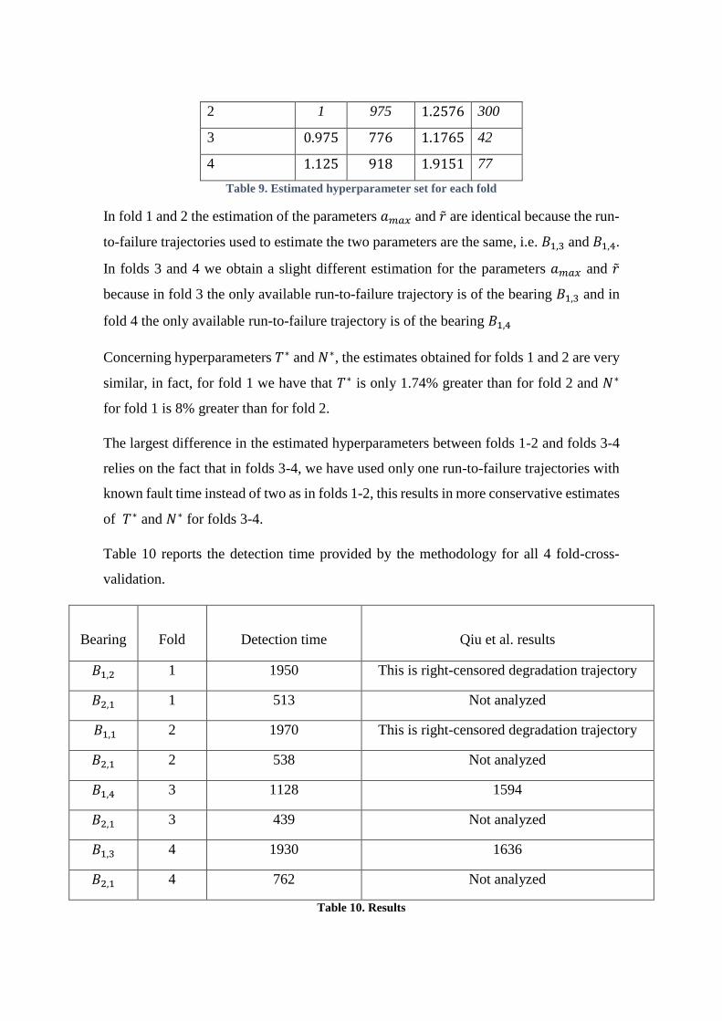
2 1 975 1.2576 300
3 0.975 776 1.1765 42
4 1.125 918 1.9151 77
Table 9. Estimated hyperparameter set for each fold
In fold 1 and 2 the estimation of the parameters 𝑎𝑚𝑎𝑥 and �̃� are identical because the run-
to-failure trajectories used to estimate the two parameters are the same, i.e. 𝐵1,3 and 𝐵1,4.
In folds 3 and 4 we obtain a slight different estimation for the parameters 𝑎𝑚𝑎𝑥 and �̃�
because in fold 3 the only available run-to-failure trajectory is of the bearing 𝐵1,3 and in
fold 4 the only available run-to-failure trajectory is of the bearing 𝐵1,4
Concerning hyperparameters 𝑇∗ and 𝑁∗, the estimates obtained for folds 1 and 2 are very
similar, in fact, for fold 1 we have that 𝑇∗ is only 1.74% greater than for fold 2 and 𝑁∗
for fold 1 is 8% greater than for fold 2.
The largest difference in the estimated hyperparameters between folds 1-2 and folds 3-4
relies on the fact that in folds 3-4, we have used only one run-to-failure trajectories with
known fault time instead of two as in folds 1-2, this results in more conservative estimates
of 𝑇∗ and 𝑁∗ for folds 3-4.
Table 10 reports the detection time provided by the methodology for all 4 fold-cross-
validation.
Bearing
Fold
Detection time
Qiu et al. results
𝐵1,2 1 1950 This is right-censored degradation trajectory
𝐵2,1 1 513 Not analyzed
𝐵1,1 2 1970 This is right-censored degradation trajectory
𝐵2,1 2 538 Not analyzed
𝐵1,4 3 1128 1594
𝐵2,1 3 439 Not analyzed
𝐵1,3 4 1930 1636
𝐵2,1 4 762 Not analyzed
Table 10. Results
The bearing 𝐵2,1 has a stable detection in all the folds but the 4. This bearing is a run-to-
failure trajectory and we detects an alarm in all the folds. The bearings 𝐵1,2 and 𝐵1,1 is
are right-censored degradation trajectories and we detect an alarm only at the end of the
test, from segments 1950 and 1970 respectively. We consider these results for the
bearings 𝐵1,2 and 𝐵1,1 to be reasonable, in fact, be taking into account the degradation
process.
For the bearing 𝐵1,4 we detect a stable alarm starting from the segments 1128, in (Qiu et
al., 2006) the fault was detect only from the segments 1594. For the bearing 𝐵1,3 we detect
the alarm only at the end of the test, at segment 1930, in (Qiu et al., 2006) the alarm is
detected from the segments 1636. The results for bearing 𝐵1,4 and 𝐵1,3 are obtanied
having in the validation set only one run-to-failure trajectory, then a less favorable
scenario than in folds 1 and 2
3.6 Chapter conclusions
In this chapter, we have developed a novel method for bearing fault detection, which
combines the use of CWT with an image analysis technique. Fault detection is performed
by comparing the CWT scalograms obtained from the test signal with those obtained from
historical data of the same bearing in healthy condition. The proposed method has been
tested using the data from real run-to-failure tests. The method has shown to give
reasonable results for the right-censored degradation trajectories, giving the alarm only at
the end of the run-to-failure test, and has shown to be able to detect the degradation onset
for the run-to-failure trajectories before the occurrence of the fault.


4 Conclusions
In this thesis work we have developed a fault detection method when the monitored
signals are nonstationary. The developed method is based on the following three steps:
1. performing the CWT of the test signal;
2. computing the corresponding scalogram image;
3. comparing this scalogram with those obtained from historical data;
With respect to the choice of the type of wavelet transform, we resort to the Morlet, a
wavelet that is well suited for our analysis. After the second step, the scalogram image of
the test signal is processed processed order to: i) enhance the differences between the
scalogram of signals recorded in nominal condition and the scalogram of signals that have
anomalous behavior; ii) normalize the entries of the scalogram in the range [0, 1].
With respect to the step 3, the comparison between scalogram images is performed by
defining a proper measure of similarity between images based on a pixel by pixel
comparison and, finally, the test signal is then classified as anomalous or non-anomalous.
The practical industrial benefit of the technique is a visual representation of fault
detection.
The proposed method was firstly applied to a real industrial case study concerning the
identification of anomalous signals recorded by a sensor, i.e. sensor data validation.
Several types of anomalies have been taken into consideration: freezing, noise, spike and
quantization, and for each one we have analyzed the effects on the scalogram image. The
underlying assumption for the sensor data validation problem are:
i. have available the historical measurements performed by the sensor itself when it
was healthy;
ii. the historical measurements are representative of all the plant operating
conditions.
The performance of the method, measured in terms of false and missed alarm rates, is
shown superior to that of a PCA-based approach for data validation, with a good
robustness considering different intensities of the malfunctions. Moreover, the method
doesn’t take advantage of correlations among plant signals, making it easily applicable to

all the sensors of a fleet of plants without requiring sensor grouping, being the validation
of the data measured from a sensor independent to that of other sensors.
The second industrial case concerns the application of the method to the bearings
degradation onset detection. The detection of the bearing degradation onset is based on
the analysis of the test pattern and comparing it with the historical measurements of the
same bearing when it was healthy. For setting the hyperparameters we assume to have
available historical degradation trajectories from bearings similar to the one currently
monitored. The method has shown to give reasonable results for the right-censored
degradation trajectories, giving the alarm only at the end of the run-to-failure test, and has
shown to be able to detect the degradation onset for the run-to-failure trajectories before
the occurrence of the fault.
Other possible future works would involve the extension of the method to other anomaly
detection problems such as: fault detections, system health monitoring, event detection in
sensor networks, intrusion detection and so on. Furthermore, the Morlet wavelet remained
the mother wavelet throughout the analysis, it would be interesting to optimize its shape
factor or to vary the mother wavelet itself. Finally, as an extension of the performed work,
the CWT could be used in the classification of the different abnormalities present. The
classification could be based on dictionary learning algorithm or artificial neural
networks, state of the art for image classification.
5 References
Amar, M., Gondal, I., Wilson, C. (2012). Unitary anomaly detection for ubiquitous safety
in machine health monitoring. Lecture Notes in Computer Science (including subseries
Lecture Notes in Artificial Intelligence and Lecture Notes in Bioinformatics), 7667
LNCS, pp. 361-368.
Baraldi, P., Di Maio, F., Turati, P., Zio, E. (2015). Robust signal reconstruction for
condition monitoring of industrial components via a modified Auto Associative Kernel
Regression method. Mechanical Systems and Signal Processing, 60, pp. 29-44.

Baraldi, P., Cannarile, F., Di Maio, F., Zio, E. (2016). Hierarchical k-nearest
neighbours classification and binary differential evolution for fault diagnostics of
automotive bearings operating under variable conditions. Engineering Applications of
Artificial Intelligence, 56, pp. 1-13.
Baraldi, P., Gola, G., Zio, E., Roverso, D., Hoffmann, M. (2011). A randomized model
ensemble approach for reconstructing signals from faulty sensors. Expert Systems with
Applications, 38 (8), pp. 9211-9224.
Baraldi, P., Mangili, F., Gola, G., Nystad, B.H., Zio, E., (2014). A hybrid ensemble-
based approach for process parameter estimation and degradation assessment in
offshore oil platforms. International Journal of Performability Engineering, 10 (5), pp.
497-509.
Baraldi, P., Zio, E., Gola, G., Roverso, D., Hoffmann, M., (2011). Two novel
procedures for aggregating randomized model ensemble outcomes for robust signal
reconstruction in nuclear power plants monitoring systems. Annals of Nuclear Energy,
38 (2-3), pp. 212-220.
Bellini, A., Immovilli, F., Rubini, R., Tassoni, C. (2008). Diagnosis of bearing faults in
induction machines by vibration or current signals: A critical comparison. Conference
Record - IAS Annual Meeting (IEEE Industry Applications Society), art. no. 4658814
Blodt, M., Granjon, P., Raison, B., Rostaing, G. (2008). Models for bearing damage
detection in induction motors using stator current monitoring IEEE Transactions on
Industrial Electronics, 55 (4), pp. 1813-1822.
Boufenar, M., Rechak, S. (2013). An enhanced technique for roller bearing defect
detection using an impulse response wavelet based sparse code shrinkage de-noising
algorithm. 2013 8th International Workshop on Systems, Signal Processing and Their
Applications, WoSSPA 2013, art. no. 6602400, pp. 407-412.
Cannarile, F., Baraldi, P., Compare, M., Zio, E., (2017). An unsupervised clustering
method for assessing the degradation state of cutting tools in the packaging industry.
Safety and Reliability: Theory and Application- Proceedings of the European Safety and
Reliability Conference, ESREL 2017, accepted.
Chebil, J., Noel, G., Mesbah, M., Deriche, M. (2009). Wavelet decomposition for the
detection and diagnosis of faults in rolling element bearings. Jordan Journal of
Mechanical and Industrial Engineering, 3 (4), pp. 260-267.
Coble, J.B., Meyer, R.M., Ramuhalli, P., Bond, L.J., Hashemian, H., Shumaker, B., et
al., 2012. A Review of Sensor Calibration Monitoring for Calibration Interval Extension
in Nuclear Power Plants. Pacific Northwest National Laboratory.
Gao, R. X., Yan, R., (2011). Wavelets: Theory and Applications for Manufacturing.
Wavelets: Theory and Applications for Manufacturing, pp. 1-224.
Gao, R. X, Yan, R. (2011). Wavelets Theory and Applications for Manufacturing.
Springer Science & Business Media.
Garvey, J., Garvey, D., Seibert, R., Hines, J.W. (2007). Validation of on-line monitoring
techniques to nuclear plant data. Nucl. Eng. Tech., 39 (2), pp. 149-158.
Gross, K.C., Singer, R.M., Wegerich, S.W., Herzog, J.P. (1997). Application of a
model-based fault detection system to nuclear plant signals. Proceedings of the
intelligent system applications to power systems, ISAP, Seoul, Korea, pp 66–70.
Hines, J.W., Uhrig, R.E., Wrest, D.J., (1998) Use of autoassociative neural networks for
signal validation. Journal of Intelligent and Robotic System, 21, pp. 143-154.

Holschneider, M., Tchamitchian, P., (1989). Regularite locale de la fonction non-
differentiable de Riemann. Les ondelettes en 1989, Lecture notes in Mathematics, P. G.
Lemarie, Ed. NewYork: Springer-Verlag, 1989.
Jacop, A., Khang, H. V., Robbersmyr, Kjell. G., Cardoso, A. J. M. (2017). Bearing fault
detection for drivetrains using adaptive filters based wavelet transform 20th
International Conference on Electrical Machines and Systems
Jiang, H., Wang, H., Zhou, Y. (2014). An optimal lifting multiwavelet for rotating
machinery fault detection Journal of Vibroengineering, 16 (1), pp. 303-311.
Kai, S., Jianmin, G., Zhiyong, G., Hongquan, J., Xu, G., (2015). Plant-wide quantitative
assessment of a process industry system's operating state based on color-spectrum.
Mechanical Systems and Signal Processing, 60, pp. 644-655.
Karacan, C.O., Olea, R.A., (2014). Inference of strata separation and gas emission
paths in longwall overburden using continuous wavelet transform of well logs and
geostatistical simulation. Journal of Applied Geophysics, 105, pp. 147-158.
Kovačević, J., Chebira, A., (2007a) Life beyond bases: The advent of frames (Part I).
IEEE Signal Processing Magazine, 24 (4), pp. 86-104.
Kovačević, J., Chebira, A. (2007 b). Life beyond bases: The advent of frames (Part II)
IEEE Signal Processing Magazine, 24 (5), pp. 115-125.
Lee, J.-M., Yoo, C.K., Choi, S.W., Vanrolleghem, P.A., Lee, I.-B, (2004). Nonlinear
process monitoring using kernel principal component analysis. Chemical Engineering
Science, 59 (1), pp. 223-234.
Li, B., Chow, M.-Y., Tipsuwan, Y., Hung, J.C. (2000). Neural-network-based motor
rolling bearing fault diagnosis IEEE Transactions on Industrial Electronics, 47 (5), pp.
1060-1069.
Li, H., (2010) Gear Fault Diagnosis Based on Continuous Morlet Wavelet Amplitude
and PhaseMap. Seventh International Conference on Fuzzy Systems and Knowledge
Discovery 2010, 6, pp. 2619-2622.
Lin, J., Qu, L. (2000). Feature extraction based on morlet wavelet and its application
for mechanical fault diagnosis Journal of Sound and Vibration, 234 (1), pp. 135-148.
Mallat, S., (2008). A Wavelet Tour of Signal Processing. Third edition Academic Press,
published 11 December 2008.
Mallat, S., Hwang, W.L., (1992). Singularity detection and processing with wavelets.
IEEE Transactions on Information Theory, 38 (2), pp. 617-643.
Miao, Q., Huang, H.-Z., Fan, X., (2007). Singularity detection in machinery health
monitoring using Lipschitz exponent function. Journal of Mechanical Science and
Technology, 21 (5), pp. 737-744.
Ni, K., Ramanathan, N., Chehade, M.N.H., Balzano, L., Nair, S., Zahedi, S., Kohler, E.,
Pottie, G., Hansen, M., Srivastava, M., (2009). Sensor network data fault types. ACM
Transactions on Sensor Networks, 5 (3), pp. 1-29.
Penha, R., Hines, J., (2001). Using principal component analysis modeling to monitor
temperature sensors in a nuclear research reactor. Maintenance and reliability
conference (MARCON 2001).
Peng, Z., He, Y., Chen, Z., Chu, F., (2002). Identification of the shaft orbit for rotating
machines using wavelet modulus maxima. Mechanical Systems and Signal Processing,
16 (4), pp. 623-635.
Qiu, H., Lee, J., Lin, J., Yu, G., (2006). Wavelet filter-based weak signature detection
method and its application on rolling element bearing prognostics. Journal of Sound
and Vibration, Volume 289, (4-5), pp. 1066-1090.
Rasmussen, B., Hines, J.W., Uhrig, R.E., (2000). Nonlinear partial least squares
modeling for instrument surveillance and calibration verification. Proceedings of the
maintenance and reliability conference (MARCON 2000).
Roverso, D., Hoffmann, M., Zio, E., Baraldi, P., Gola, G., (2007). Solutions for plant-
wide on-line calibration monitoring. Proceedings of the European Safety and Reliability
Conference 2007, ESREL 2007 - Risk, Reliability and Societal Safety.
Sengüler, T., Seker, S., (2016). Continuous wavelet transform for ferroresonance
detection in power systems. Electrical Engineering, 99 (2), pp. 595-600.
Sharma, A.B., Golubchik, L., Govindan, R., (2010). Sensor faults: Detection methods
and prevalence in real-world datasets. ACM Transactions on Sensor Networks, 6 (3),
art. no. 23.
Struzik, Z.R., (2001). Wavelet methods in (financial) time-series processing. Physica A:
Statistical Mechanics and its Applications, 296 (1-2), pp. 307-319.
Tolle, G., Polastre, J., Szewczyk, R., Culler, D., Turner, N., Tu, K., Burgess, S.,
Dawson, T., Buonadonna, P., Gay, D., and Hong, W., (2005). A Macroscope in the
Redwoods. Proceedings of the 2nd international conference on Embedded networked
sensor systems (SenSys), pp. 51–63.
Torrence, C., Compo, G.P., (1998). A Practical Guide to Wavelet Analysis. Bulletin of
the American Meteorological Society, 79 (1), pp. 61-78.
Tu, C.-L., Hwang, W.-L., Ho, J., (2005). Analysis of singularities from modulus maxima
of complex wavelets. IEEE Transactions on Information Theory, 51 (3), pp. 1049-1062.
Wegener, I., (2005). Complexity theory: Exploring the limits of efficient algorithms.
Complexity Theory: Exploring the Limits of Efficient Algorithms, pp. 1-308.
Wrest, D.J., Hines, J.W., Uhrig, R.E., (1996). Instrument surveillance and calibration
verification through plant wide monitoring using autoassociative neural networks. In
the proceedings of the 1996 American nuclear society international topical meeting on
nuclear plant instrumentation, Control and human machine interface technologies, pp 6–
9.
Yang, Y., Tang, W. (2011) Study of remote bearing fault diagnosis based on BP Neural
Network combination Proceedings - 2011 7th International Conference on Natural
Computation, ICNC 2011, 2, art. no. 6022177, pp. 618-621.
Zavaljevskiz N., Gross, K.C. (2000). Sensor fault detection in nuclear power plants
using multivariate state estimation technique and support vector machines. 3rd
International Conference of the Yugoslav Nuclear Society.
Zhao, C.-Y., Ning, P., Liu, B.-Y., Wang, L., Ni, X.-L., Ma, L. (2013). Best Morlet
wavelet-based full information energy entropy extraction with its application to rolling
bearing condition monitoring QR2MSE 2013 - Proceedings of 2013 International
Conference on Quality, Reliability, Risk, Maintenance, and Safety Engineering, art. no.
6625928, pp. 1808-1811.


6 Appendices A: Continuous Wavelet Transform
In mathematical terms, a wavelet is a function 𝜓(𝑡) ∈ 𝐿2(ℝ)satisfying the admissibility
condition (Mallat & Hwang, 1992):
∫|𝜉(𝜔)|2
𝜔𝑑𝜔 = ∫
|𝜉(𝜔)|2
|𝜔|𝑑𝜔 = 𝐶
0
−∞
< ∞+∞
0
(24)
where 𝐿2(ℝ) denotes the space of square-integrable functions and 𝜉(𝜔) the Fourier
transform of the wavelet function 𝜓(𝑡). The admissibility condition implies that the
Fourier transform of the function 𝜓(𝑡) vanishes at zero frequency:
|𝜉(𝜔)|𝜔=02= 0 (25)
and that the average value of the wavelet 𝜓(𝑡) is zero (Mallat & Hwang, 1992):
∫ 𝜓(𝑡)𝑑𝑡 = 0+∞
−∞
(26)
A dictionary of time-frequency atoms is defined from the wavelet function 𝜓(𝑡) by
scaling 𝜓(𝑡) by 𝑠 (referred to as the scale parameter) and translating it by 𝑢 (referred to
as translation parameter):
𝜓𝑢,𝑠(𝑡): =1
√𝑠𝜓 (
𝑡 − 𝑢
𝑠) 𝑢 ∈ ℝ, 𝑠 > 0 (27)
For any real signal 𝑥(𝑡) ∈ 𝐿2(ℝ), the Continuous Wavelet Transform (CWT) with scale
parameter 𝑠 and translation parameter 𝑢 is:
𝐶𝑊𝑇𝑥𝜓(𝑢, 𝑠) = ∫ 𝑥(𝑡)𝜓𝑢,𝑠(𝑡)𝑑𝑡
+∞
−∞
(28)
The factor 1
√𝑠 in Eq. (27) guarantees that the wavelet transform in Eq. (1) and Eq.(11) is
directly comparable at different scales.
7 Appendix B: Lipschitz exponent
A function 𝑥(𝑡) is pointwise Lipschitz 𝛼 ≥ 0 at 𝑡0, if there exist 𝐴 > 0 and a polynomial
𝑃𝑡0 of degree 𝑛𝛼 = ⌊𝛼⌋ , the greatest integer less than or equal to 𝛼, such that (Mallat,
2008):
|𝑥(𝑡) − 𝑃𝑡0 (𝑡)| ≤ 𝐴|𝑡 − 𝑡0|𝛼 ∀𝑡𝜖ℝ (29)
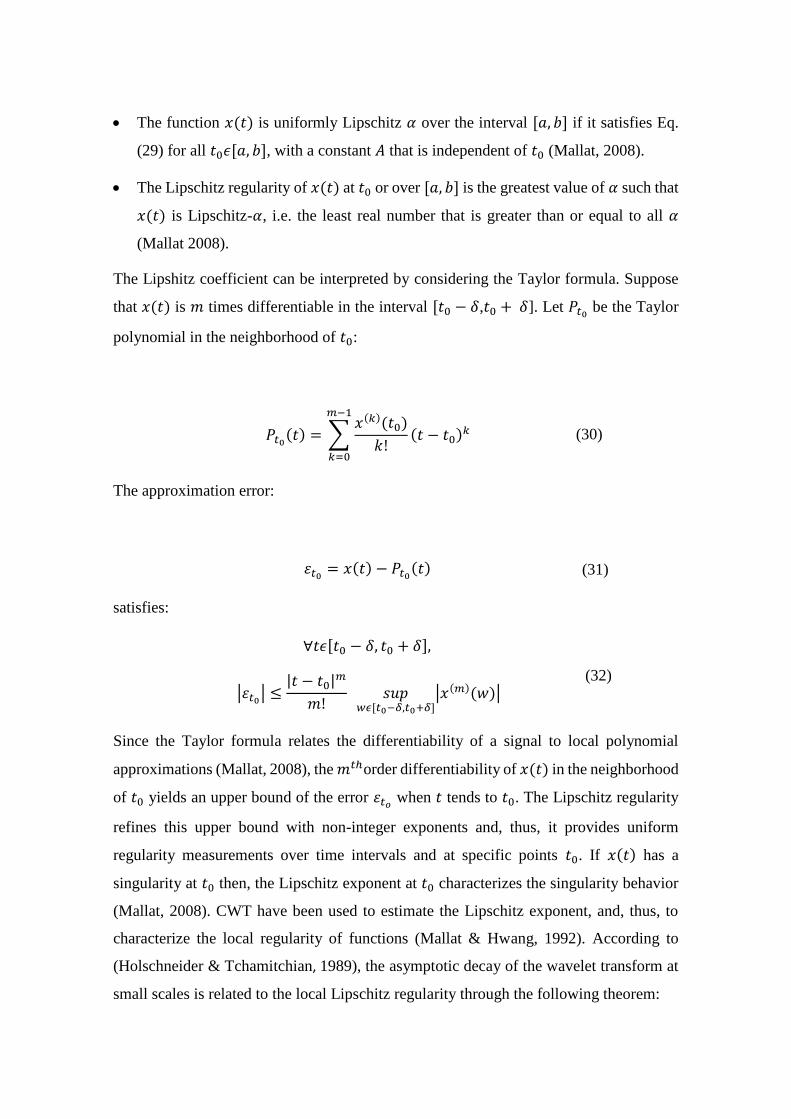
• The function 𝑥(𝑡) is uniformly Lipschitz 𝛼 over the interval [𝑎, 𝑏] if it satisfies Eq.
(29) for all 𝑡0𝜖[𝑎, 𝑏], with a constant 𝐴 that is independent of 𝑡0 (Mallat, 2008).
• The Lipschitz regularity of 𝑥(𝑡) at 𝑡0 or over [𝑎, 𝑏] is the greatest value of 𝛼 such that
𝑥(𝑡) is Lipschitz-𝛼, i.e. the least real number that is greater than or equal to all 𝛼
(Mallat 2008).
The Lipshitz coefficient can be interpreted by considering the Taylor formula. Suppose
that 𝑥(𝑡) is 𝑚 times differentiable in the interval [𝑡0 − 𝛿,𝑡0 + 𝛿]. Let 𝑃𝑡0 be the Taylor
polynomial in the neighborhood of 𝑡0:
𝑃𝑡0(𝑡) = ∑𝑥(𝑘)(𝑡0)
𝑘!(𝑡 − 𝑡0)
𝑘
𝑚−1
𝑘=0
(30)
The approximation error:
휀𝑡0 = 𝑥(𝑡) − 𝑃𝑡0(𝑡) (31)
satisfies:
∀𝑡𝜖[𝑡0 − 𝛿, 𝑡0 + 𝛿],
|휀𝑡0| ≤|𝑡 − 𝑡0|
𝑚
𝑚! 𝑠𝑢𝑝𝑤𝜖[𝑡0−𝛿,𝑡0+𝛿]
|𝑥(𝑚)(𝑤)| (32)
Since the Taylor formula relates the differentiability of a signal to local polynomial
approximations (Mallat, 2008), the 𝑚𝑡ℎorder differentiability of 𝑥(𝑡) in the neighborhood
of 𝑡0 yields an upper bound of the error 휀𝑡𝑜 when 𝑡 tends to 𝑡0. The Lipschitz regularity
refines this upper bound with non-integer exponents and, thus, it provides uniform
regularity measurements over time intervals and at specific points 𝑡0. If 𝑥(𝑡) has a
singularity at 𝑡0 then, the Lipschitz exponent at 𝑡0 characterizes the singularity behavior
(Mallat, 2008). CWT have been used to estimate the Lipschitz exponent, and, thus, to
characterize the local regularity of functions (Mallat & Hwang, 1992). According to
(Holschneider & Tchamitchian, 1989), the asymptotic decay of the wavelet transform at
small scales is related to the local Lipschitz regularity through the following theorem:
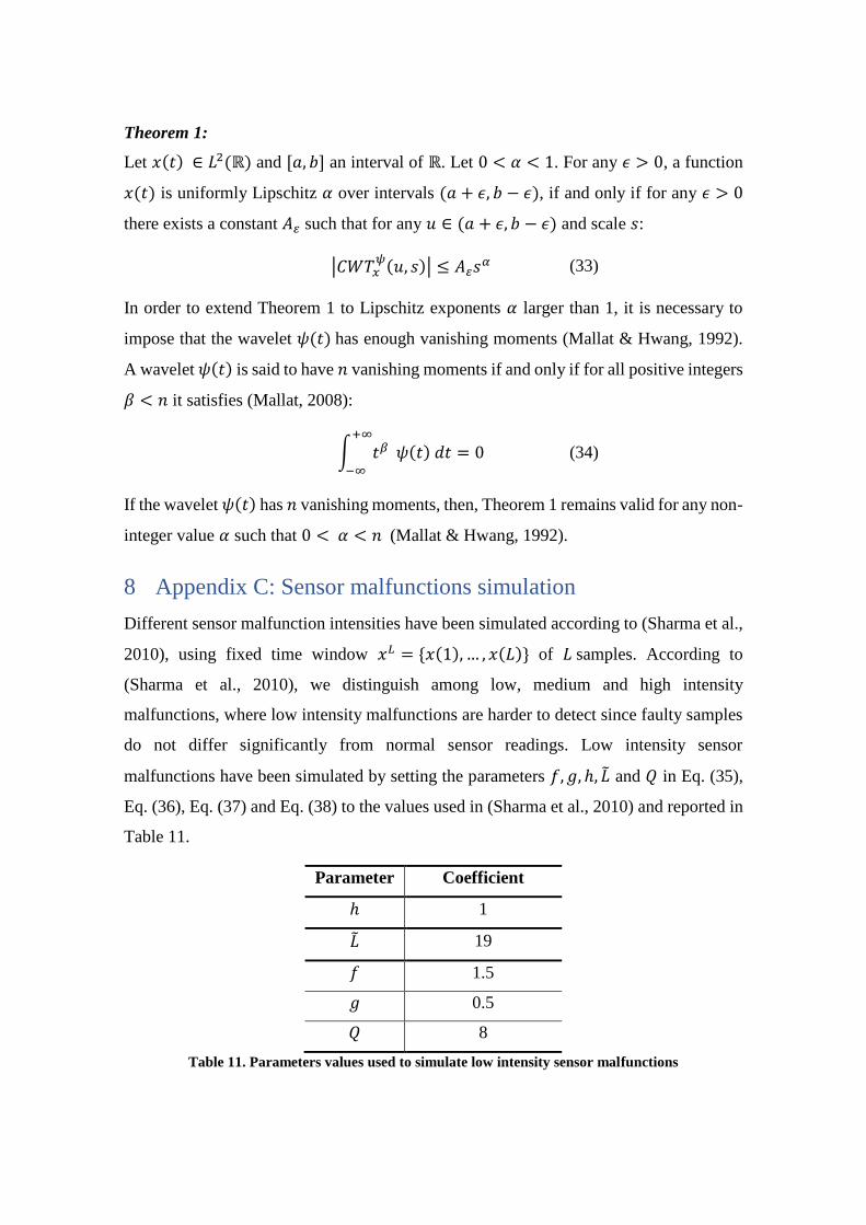
Theorem 1:
Let 𝑥(𝑡) ∈ 𝐿2(ℝ) and [𝑎, 𝑏] an interval of ℝ. Let 0 < 𝛼 < 1. For any 𝜖 > 0, a function
𝑥(𝑡) is uniformly Lipschitz 𝛼 over intervals (𝑎 + 𝜖, 𝑏 − 𝜖), if and only if for any 𝜖 > 0
there exists a constant 𝐴 such that for any 𝑢 ∈ (𝑎 + 𝜖, 𝑏 − 𝜖) and scale 𝑠:
|𝐶𝑊𝑇𝑥𝜓(𝑢, 𝑠)| ≤ 𝐴 𝑠𝛼 (33)
In order to extend Theorem 1 to Lipschitz exponents 𝛼 larger than 1, it is necessary to
impose that the wavelet 𝜓(𝑡) has enough vanishing moments (Mallat & Hwang, 1992).
A wavelet 𝜓(𝑡) is said to have 𝑛 vanishing moments if and only if for all positive integers
𝛽 < 𝑛 it satisfies (Mallat, 2008):
∫ 𝑡𝛽+∞
−∞
𝜓(𝑡) 𝑑𝑡 = 0 (34)
If the wavelet 𝜓(𝑡) has 𝑛 vanishing moments, then, Theorem 1 remains valid for any non-
integer value 𝛼 such that 0 < 𝛼 < 𝑛 (Mallat & Hwang, 1992).
8 Appendix C: Sensor malfunctions simulation
Different sensor malfunction intensities have been simulated according to (Sharma et al.,
2010), using fixed time window 𝑥𝐿 = {𝑥(1), … , 𝑥(𝐿)} of 𝐿 samples. According to
(Sharma et al., 2010), we distinguish among low, medium and high intensity
malfunctions, where low intensity malfunctions are harder to detect since faulty samples
do not differ significantly from normal sensor readings. Low intensity sensor
malfunctions have been simulated by setting the parameters 𝑓, 𝑔, ℎ, �̃� and 𝑄 in Eq. (35),
Eq. (36), Eq. (37) and Eq. (38) to the values used in (Sharma et al., 2010) and reported in
Table 11.
Parameter Coefficient
ℎ 1
�̃� 19
𝑓 1.5
𝑔 0.5
𝑄 8
Table 11. Parameters values used to simulate low intensity sensor malfunctions

To simulate medium and high intensity malfunctions the parameters 𝑓, 𝑔, ℎ and 𝑄 in Eq.
(35), Eq. (36), Eq. (37) and Eq. (38), have been set as in (Sharma et al., 2010) and are
reported in Table 12.
Parameters Coefficient for medium
intensity
Coefficient for
high intensity
ℎ 1 1
�̃� 40 80
𝑓 5 10
𝑔 1.5 3
𝑄 6 3
Table 12. Parameters values used to simulate low intensity sensor malfunctions
• Spike
Spike malfunctions have been simulated by randomly drawing a sample 𝑟 and
replacing the reported value 𝑥(𝑘) with
�̃�(𝑟) = 𝑥(𝑟) + 𝑓𝑥(𝑟) (35)
where the multiplicative factor 𝑓 determines the intensity of the spike faults.
• Noise
Noise malfunctions have been simulated selecting a set of successive samples
𝑊and added a random draw from a normal distribution, 𝑁(0, 𝑔2𝜎2), to each
sample 𝑥(𝑟) in 𝑊, i.e.,
�̃�(𝑟) = 𝑥(𝑟) + √𝑔2𝜎2𝑁(0,1) (36)
where 𝜎2 is the variance of the signal in nominal condition and 𝑔 is a
multiplicative factor, which allows controlling the intensity of noise malfunctions.
• Freezing
Freezing malfunctions have been simulated selecting the time length �̃� < 𝐿 for
which the signal measurement is affected by freezing, randomly drawing the time
of occurrence of the malfunction �̃� = 1,… , 𝐿 − �̃�, and replacing the sensor
reading with

�̃�(𝑟) = 𝑥(�̃�) + ℎ 𝑟 = �̃�, … , �̃� + �̃� − 1 (37)
where ℎ indicates the size of the sudden jump at the beginning of the freezing.
• Quantization
To inject quantization faults, we have firstly computed the minimum 𝑚𝑖𝑛 and the
maximum 𝑚𝑎𝑥 values within the time window 𝑥𝐿; then, we have selected the
number 𝑄 of discrete levels, so that the possible values that the quantized signal
can assume are
𝑦𝑙 = (𝑙 − 1) (𝑚𝑎𝑥 −𝑚𝑖𝑛
𝑄) +𝑚𝑖𝑛 𝑙 = 1,… , 𝑄 (38)
Finally, the reported value 𝑥(𝑟) is replaced with 𝑦𝑞∗(𝑟), where the index 𝑞∗(𝑟)
satisfies
𝑞∗(𝑟) = 𝑎𝑟𝑔𝑚𝑖𝑛𝑞=1,…,𝑄|𝑦𝑙 − 𝑥(𝑟)| (39)

Ringraziamenti
Desidero ringraziare il Prof. Piero Baraldi per la guida in questo progetto, per avermi
mostrato il metodo ed il rigore necessario per fare ricerca scientifica condividendo idee e
consigli utili per il mio lavoro.
Ringrazio il Prof. Enrico Zio per l’opportunità concessami di svolgere il lavoro di tesi con
lui, per avermi proposto un argomento di ricerca in un campo che mi ha subito
appassionato e che ho potuto scoprire e studiare in ogni giorno di questo lavoro.
Ringrazio Francesco per l’aiuto quotidiano che ha saputo darmi durante tutto il periodo
di tesi, per le spiegazioni al telefono lunghissime e per le discussioni in ufficio ad orari
improbabili (NON SI CAPISCE, RISCRIVI MEGLIO)
Ringrazio tutta mia famiglia, mio papà, mia mamma e mio fratello per il supporto e per
l’opportunità che mi hanno dato per seguire questo percorso non proprio lineare.
Non ultimi ringrazio tutti i miei amici, di Termoli, di Milano, Matematici, Meccanici,
aerospaziali, elettronici, nucleari e chi più ne ha più ne metta.


