Plug‐in Hybrid Powertrain Configuration C i U i Gl b l O i i iComparison Using Global Optimization
SAE 2009‐01‐1334
April 2009
Dominik Karbowski, Karl‐Felix Freiherr von Pechmann
Sylvain Pagerit, Jason Kwon, Aymeric RousseauArgonne National Laboratory
Sponsored by Lee Slezakp y
This presentation does not contain any proprietary, confidential, or otherwise restricted information
PHEVs Come in Various Powertrain Configurations: How to Compare Them?Configurations: How to Compare Them? Series, Parallel, Power‐split, etc.
Prototypes exist but built upon different requirements Prototypes exist, but built upon different requirements, sizes, electric ranges, etc.
PHEV control allows for much freedom in the power split
Simulation tools allows comparison on common grounds: Forward‐looking, such as Argonne’s PSAT
• Mimics real‐world chain of decision includes transient drivability• Mimics real‐world chain of decision, includes transient, drivability features
• Rule‐based controls need to be tuned
Global Optimization/Dynamic Programming Global Optimization/Dynamic Programming• Backward‐looking and cycle‐dependent approach makes this a theoretical tool
• Control is an output, each vehicle operates “at its best”p , p
Global optimization is ideal tool for “fair” comparison
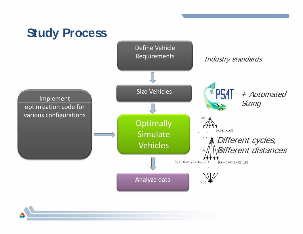
Study ProcessDefine Vehicle Requirements Industry standards
Size VehiclesImplement + Automated
Sizing
Optimally Si l t
optimization code for various configurations
Sizing
tSOCtP nm ,
0X
Simulate Vehicles
nm
tJtSOCtP 11
tU0 tU M
...
Different cycles,Different distances
Analyze data
tJtSOCtP '0,000 ,1',1 tJtSOCtP MMMM ',' ,1,1
TX
...
Outline
Vehicle Sizing
Global Optimization Algorithm
Simulation Results
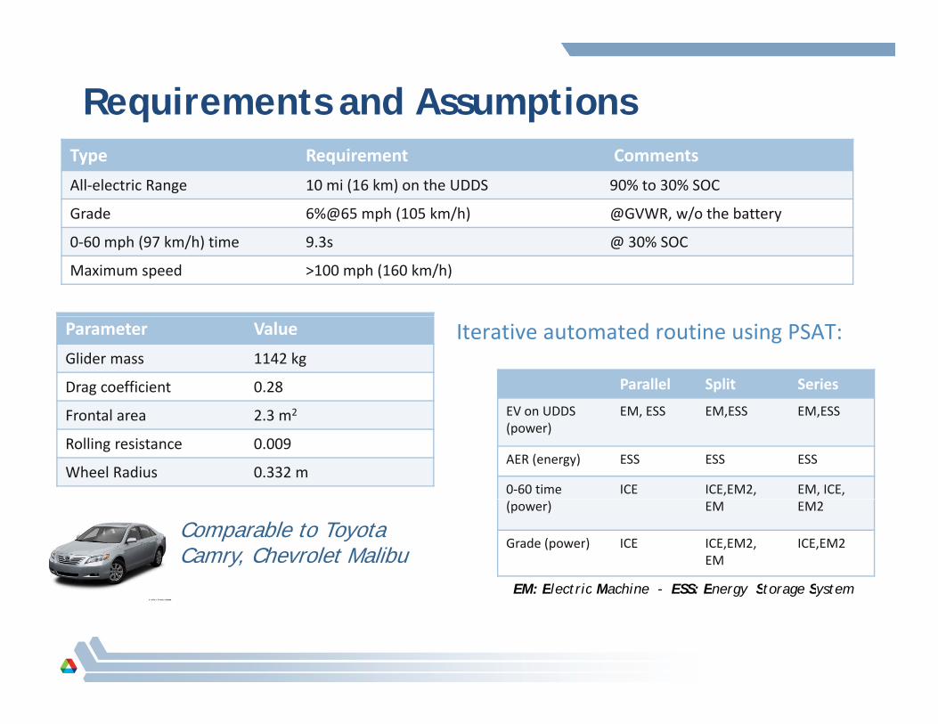
Requirements and AssumptionsType Requirement Comments
All‐electric Range 10 mi (16 km) on the UDDS 90% to 30% SOC
Grade 6%@65 mph (105 km/h) @GVWR, w/o the battery
0‐60 mph (97 km/h) time 9.3s @ 30% SOC
Maximum speed >100 mph (160 km/h)
Parameter Value
Glider mass 1142 kg
Drag coefficient 0.28
Iterative automated routine using PSAT:
Parallel Split Series
EV UDDS EM ESS EM ESS EM ESSFrontal area 2.3 m2
Rolling resistance 0.009
Wheel Radius 0.332 m
EV on UDDS (power)
EM, ESS EM,ESS EM,ESS
AER (energy) ESS ESS ESS
0‐60 time ICE ICE,EM2, EM, ICE,
Comparable to Toyota Camry, Chevrolet Malibu
(power) EM EM2
Grade (power) ICE ICE,EM2,EM
ICE,EM2
EM: Electric Machine - ESS: Energy Storage SystemEM: Electric Machine ESS: Energy Storage System
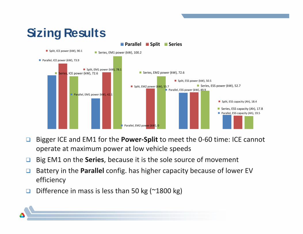
Sizing ResultsParallel Split Series
Parallel, ICE power (kW), 73.9
Split, ICE power (kW), 90.1
Split, EM1 power (kW), 78.1Series ICE power (kW) 72 6
Series, EM1 power (kW), 100.2
Series EM2 power (kW) 72 6
Parallel Split Series
Parallel, EM1 power (kW), 42.1
Parallel, ESS power (kW), 49.9Split, EM2 power (kW), 55.7
Split, ESS power (kW), 50.5
Split, ESS capacity (Ah), 18.4
Series, ICE power (kW), 72.6 Series, EM2 power (kW), 72.6
Series, ESS power (kW), 52.7
Parallel, EM2 power (kW), 0
Parallel, ESS capacity (Ah), 19.5
Split, ESS capacity (Ah), 18.4
Series, ESS capacity (Ah), 17.8
Bigger ICE and EM1 for the Power‐Split to meet the 0‐60 time: ICE cannot operate at maximum power at low vehicle speeds
Big EM1 on the Series, because it is the sole source of movement Big EM1 on the Series, because it is the sole source of movement
Battery in the Parallel config. has higher capacity because of lower EV efficiency
Difference in mass is less than 50 kg (~1800 kg) Difference in mass is less than 50 kg ( 1800 kg)
Outline
Vehicle Sizing
Global Optimization Algorithm
Simulation Results
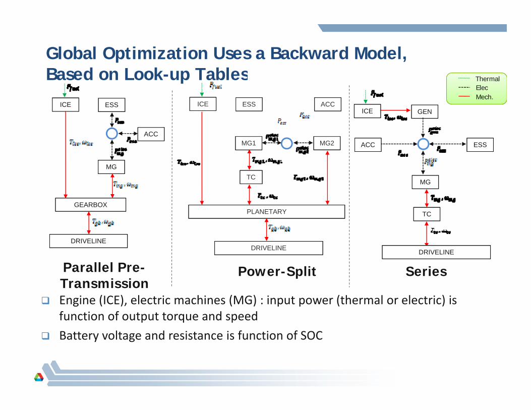
Global Optimization Uses a Backward Model, Based on Look-up TablesBased on Look-up Tables
ICE ESSICE GEN
ICE ACCESS
Thermal Elec. Mech.
ACC
MG
ACC ESSMG2MG1
TC
GEARBOX
MG
TC
TC
PLANETARY
DRIVELINEDRIVELINEDRIVELINE
Parallel Pre-Transmission
Power-Split SeriesTransmission
Engine (ICE), electric machines (MG) : input power (thermal or electric) is function of output torque and speed
Battery voltage and resistance is function of SOC Battery voltage and resistance is function of SOC
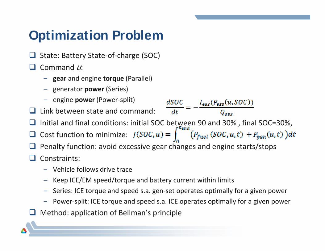
Optimization Problem State: Battery State‐of‐charge (SOC)
Command u: gear and engine torque (Parallel)– gear and engine torque (Parallel)
– generator power (Series)
– engine power (Power‐split)
Link between state and command Link between state and command:
Initial and final conditions: initial SOC between 90 and 30% , final SOC=30%,
Cost function to minimize:
Penalty function: avoid excessive gear changes and engine starts/stops
Constraints:– Vehicle follows drive trace
– Keep ICE/EM speed/torque and battery current within limits
– Series: ICE torque and speed s.a. gen‐set operates optimally for a given power
– Power‐split: ICE torque and speed s.a. ICE operates optimally for a given powerp q p p p y g p
Method: application of Bellman’s principle
Outline
Vehicle Sizing
Global Optimization Algorithm
Simulation Results
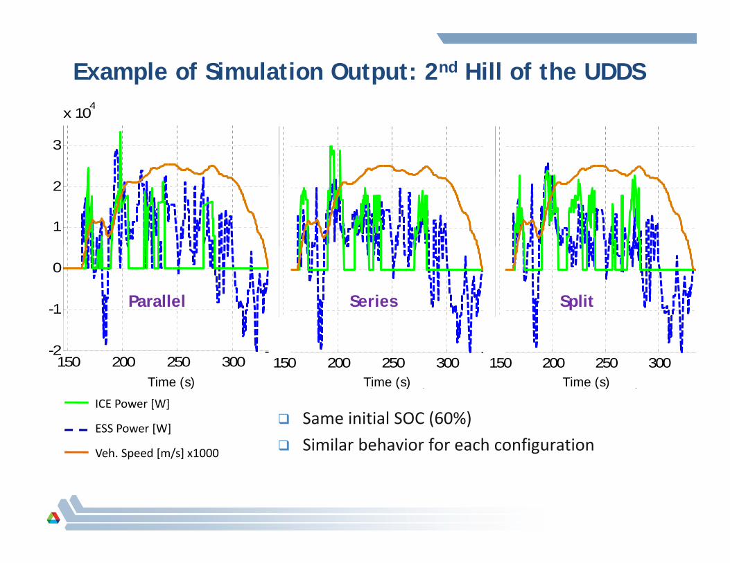
Example of Simulation Output: 2nd Hill of the UDDS4
333
x 104
1
2
1
2
1
2
-1
0
-1
0
-1
0
Parallel SplitSeries
150 200 250 300-2
time (seconds)
150 200 250 300
-2
time (seconds)
150 200 250 300-2
time (seconds)
Time (s) Time (s) Time (s)( )( )ICE Power [W]
ESS Power [W]
Veh. Speed [m/s] x1000
Same initial SOC (60%)
Similar behavior for each configuration
( ) ( ) ( )
p
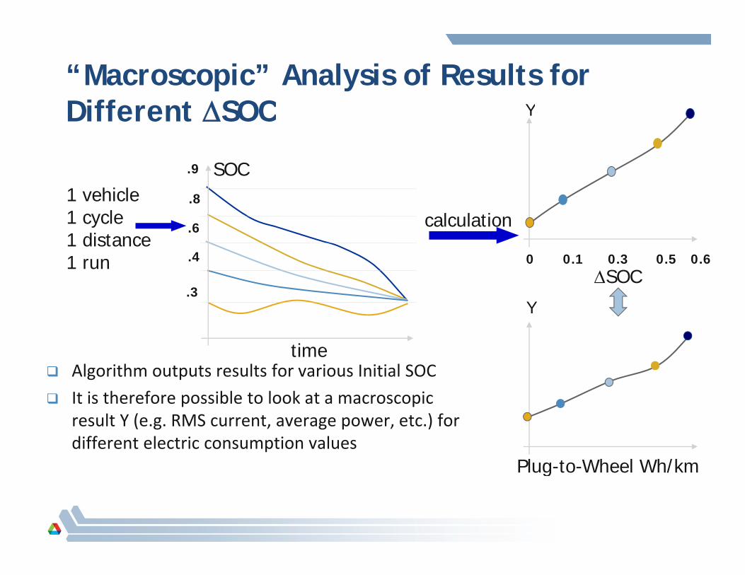
“Macroscopic” Analysis of Results for Different SOC YDifferent SOC
SOC.9
Y
1 vehicle1 cycle1 distance
calculation.8
.6
1 run .4
.3
0.60 0.1 0.3 0.5SOC
Y
time Algorithm outputs results for various Initial SOC
It is therefore possible to look at a macroscopic
Plug-to-Wheel Wh/km
It is therefore possible to look at a macroscopic result Y (e.g. RMS current, average power, etc.) for different electric consumption values
Plug to Wheel Wh/km
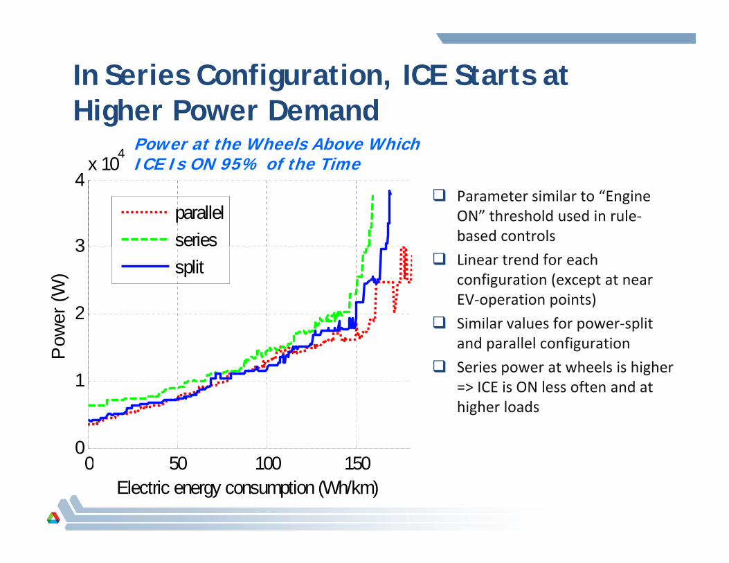
In Series Configuration, ICE Starts at High P D dHigher Power Demand
4x 10
4 Power at the Wheels Above Which ICE Is ON 95% of the Time
3
4
parallelseries
Parameter similar to “Engine ON” threshold used in rule‐based controls
2
3
er (W
)
se essplit Linear trend for each
configuration (except at near EV‐operation points)
f
1
2
Pow
e Similar values for power‐split and parallel configuration
Series power at wheels is higher => ICE is ON less often and at
0 50 100 1500
=> ICE is ON less often and at higher loadsUDDS x1
0 50 100 150Electric energy consumption (Wh/km)
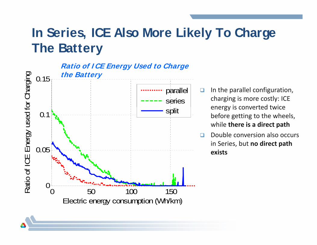
In Series, ICE Also More Likely To Charge Th B ttThe Battery
ng
Ratio of ICE Energy Used to Charge the Battery0.15
or C
harg
in parallelseries
In the parallel configuration, charging is more costly: ICE energy is converted twice
the Battery
0.1
rgy
used
fo split energy is converted twice before getting to the wheels, while there is a direct path
Double conversion also occurs
0.05
f IC
E E
ner
in Series, but no direct path existsUDDS x1
0 50 100 1500
Electric energy consumption (Wh/km)
Rat
io o
f
Electric energy consumption (Wh/km)
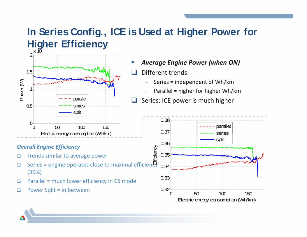
In Series Config., ICE is Used at Higher Power for Higher Efficiency Higher Efficiency
Average Engine Power (when ON)
Different trends:1.5
2x 10⁴
Different trends:– Series = independent of Wh/km
– Parallel = higher for higher Wh/km
Series: ICE power is much higher
1
Pow
er (W
)
parallel p g
0 50 100 1500
0.5
Electric energy consumption (Wh/km)
seriessplit
0.37
0.38 parallelseries
UDDS x1
Electric energy consumption (Wh/km)
0.35
0.36
0.37
Effi
cien
cy
seriessplit
Overall Engine Efficiency
Trends similar to average power
S i i t l t i l ffi i
0 50 100 1500.32
0.33
0.34E
Series = engine operates close to maximal efficiency (36%)
Parallel = much lower efficiency in CS mode
Power Split = in betweenUDDS x1
0 50 100 150Electric energy consumption (Wh/km)
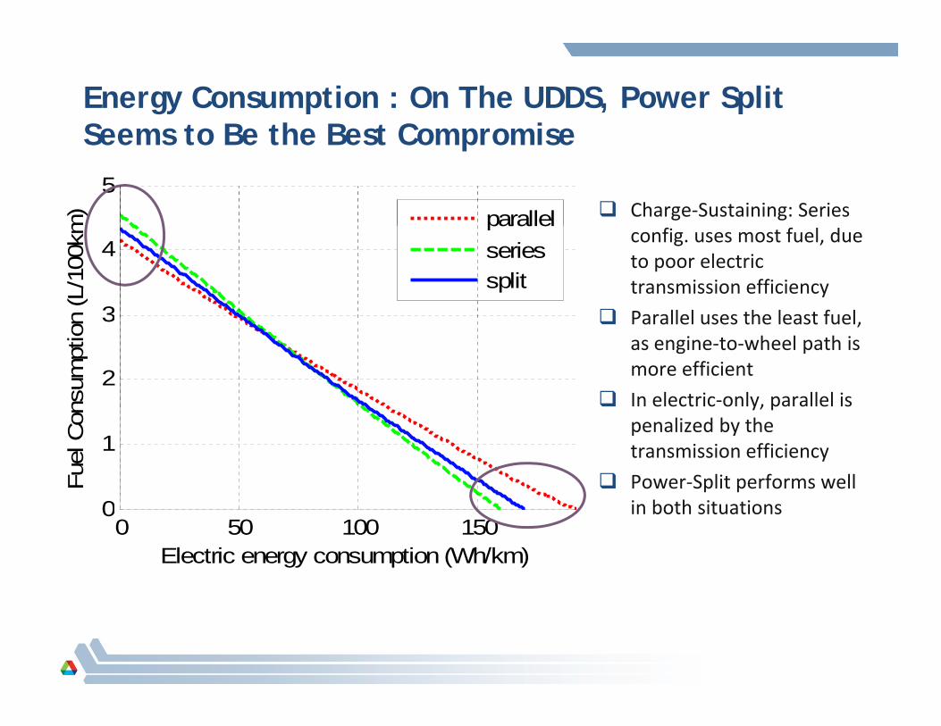
Energy Consumption : On The UDDS, Power Split Seems to Be the Best CompromiseSeems to Be the Best Compromise
Charge‐Sustaining: Series 5
m)
parallel
config. uses most fuel, due to poor electric transmission efficiency
Parallel uses the least fuel3
4
n (L
/100
km
parallelseriessplit
Parallel uses the least fuel, as engine‐to‐wheel path is more efficient
In electric‐only, parallel is 2
3
nsum
ptio
n
y, ppenalized by the transmission efficiency
Power‐Split performs well i b h i i0
1
Fuel
Con
in both situations0 50 100 150
0
Electric energy consumption (Wh/km)
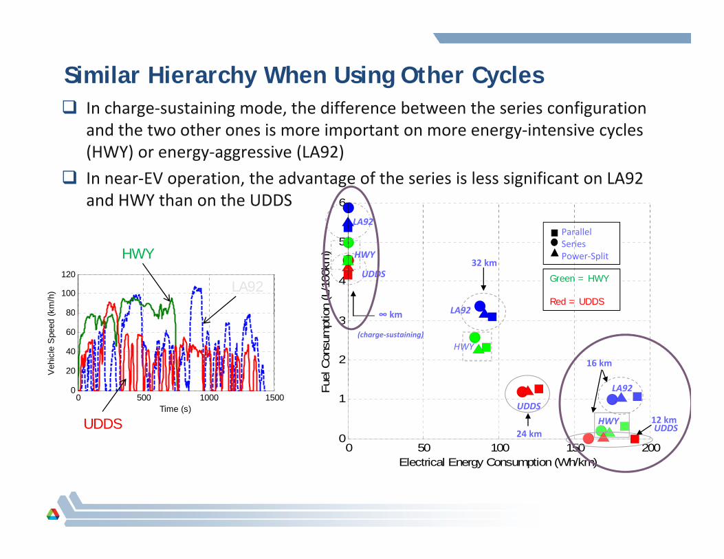
Similar Hierarchy When Using Other Cycles I h t i i d th diff b t th i fi ti In charge‐sustaining mode, the difference between the series configuration
and the two other ones is more important on more energy‐intensive cycles (HWY) or energy‐aggressive (LA92)
I EV ti th d t f th i i l i ifi t LA92
5
6
In near‐EV operation, the advantage of the series is less significant on LA92 and HWY than on the UDDS
LA92Parallel Series
4
5
on (L
/100
km)
LA92
HWY
UDDS32 km
∞ km
SeriesPower‐Split
Green = HWYBlue = LA92Red = UDDS
80
100
120
(km
/h)
HWY
LA92
2
3ue
l Con
sum
ptio
LA92
HWY
16 km
∞ km
(charge‐sustaining)
20
40
60
80
Veh
icle
Spe
ed (
0 50 100 150 2000
1
Fu
LA92
UDDS
HWYUDDS12 km
24 km
0 500 1000 15000
Time (s)
UDDS
Electrical Energy Consumption (Wh/km)
Conclusion
Comparing different powertrains requires a common set of requirements
An automated routine using PSAT allows to quickly size vehicles
Global optimization can be used to ensure “fair” comparison, because control is optimal
Series is potentiallymore efficient on the “electric‐only” side, parallel (pre‐tx) is potentiallymore efficient on the “charge‐sustaining” side, power‐split is a good compromise
Global optimization is a theoretical tool, and in real‐world optimal control is harder to get because:– it requires the knowledge of the cycle beforehand
– real‐world must also take into account drivability, safety, etc.
However it provides the theoretical boundaries, as well as control patterns
Future work will use patterns obtained from global optimization to implement adaptive rule‐based controls.


