Download - Planning Review Copy

Revie
w C
opy
Integrating CDU, FCC and Product Blending Models into Refinery
Planning
Li Wenkaia, Chi-Wai Huia,*, AnXue Lib
aChemical Engineering Department, Hong Kong University of Science and Technology,Clear Water Bay, Hong Kong
bDaqing Refining & Chemical Company, PetroChina Company Limited.
ABSTRACT
The accuracy of using linear models for crude distillation unit (CDU), fluidize-bed catalytic cracker (FCC) and
product blending in refinery planning has been debated for decades. Inaccuracy caused by nonrigorous linear
models may reduce the overall profitability or sacrifice product quality. On the other hand, using rigorous
process models for refinery planning imposes unnecessary complications on the problem because these models
lengthen the solution time and often hide critical issues and parameters for profit improvements. To overcome
these problems, this paper presents a refinery planning model that utilizes simplified empirical nonlinear process
models with considerations for crude characteristics, products’ yields and qualities, etc. The proposed model
can be easily solved with much higher accuracy than a traditional linear model. This paper will present how the
CDU, FCC and product blending models are formulated and applied to refinery planning. Several case studies
are used to illustrate the features of the refinery-planning model proposed.
Keywords: Refinery, Planning, CDU, FCC, Product Blending
1. Introduction
1.1 Two types of CDU and FCC models
Crude Distillation Unit (CDU) and Fluidize-bed Catalytic Cracking (FCC) are the major units in a refinery. To
model them, two types of modelsrigorous and empirical onesare commonly used. Rigorous models
simulate a CDU as a general distillation column, taking into account phase equilibrium, heat and mass balances
along the whole column. Results of a rigorous model include flow rates and compositions of all internal and
* Author to whom correspondence should be addressed. E-mail: [email protected]
1 of 63
Friday , June 11, 2004
Elsevier
This is the Pre-Published Version

Revie
w C
opy
external streams, and operating conditions such as tray temperatures and pressures. Considerable research has
been carried out with the aim of developing and/or improving rigorous CDU models. For example, Cechetti et
al. (1963) applied simultaneous modeling of the main column and side strippers using the θ method. Their
algorithm may fail to converge when modeling a CDU. Hess et al. (1977) extended this approach and proposed
a “Multi-θ method” to increase the convergent speed and broaden the generality of the algorithm. Russell (1983)
used a rather complicated “inside-out” class of methods to simulate CDU with good speed and wide
specifications variety. Lang et al. (1991) proposed an algorithm that integrated BP (Bubble-Point) and SR (Sum-
Rates) methods and showed that their calculated values and the experimental data were in good agreement. In
addition to these, some commercial software packages, such as Aspen Plus® (Aspentech), PRO/II® (SimSci-
Esscor) and DESIGN IITM (ChemShare), have also been developed and are commonly used. These accurate
simulation models are highly nonlinear due to the complexity of CDU.
Empirical models use empirical correlations to establish material and energy balances for CDU. First proposed
by Packie (1941), these models were further described in great detail by Watkins (1979). They are good for
preliminary designs with sufficient plant data and/or experience from previous designs (Perry et al, 1997).
Because of their simplicity, relatively easy application and adequate accuracy to reflect actual conditions of a
CDU, empirical models are suitable for overall optimization of a refinery.
Besides the CDU, FCC is another important unit that strongly influences the profitability of a refinery. Many
researchers have studied FCC models. Blanding (1953) developed a mathematical model based on a kinetic rate
expression. Jacob et al. (1976) proposed a more rigorous model using the concept of lumping groupings. These
kinetic models can be used to calculate the conversion of FCC from operation parameters such as reaction
temperature, feed composition, catalyst/oil ratio, etc. However, a planning model incorporated with these
models will be rather complicated and slow. Some correlations have been developed to obtain the yield of FCC
from simple feed properties and known conversion. Nelson (1958) and Gary et al. (2001) described different
methods to obtain the yields of FCC products by predetermined charts and figures. These correlations are very
useful for obtaining typical yields for preliminary studies and to determine the trends of product yields when
changes are made in conversion levels (Gary et al., 2001).
2 of 63
Friday , June 11, 2004
Elsevier
Revie
w C
opy
1.2 Current approaches to refinery planning
Mathematical programming has been extensively studied and implemented for long-term plant-wide refinery
planning. Although accurate results of processing units can be obtained by using rigorous models, their
complexity and the length of the solution time prevent them from being used commonly. Using rigorous models
for planning might be an overkill (Barsamian, 2001). The inefficiency of solution often hides critical issues and
parameters13. Some commercial software, such as Aspen PIMSTM (Aspentech), applied nonlinear recursion
algorithm to handle nonlinearities or provided interface to an external rigorous simulator to refinery planning.
This could be a time-consuming procedure due to the long solution time of external simulator. Zhang et al.
(2001) took into account the effect of changes in feed properties and operation conditions, using a linear
constraint with some parameters (e.g., the base yields of CDU fractions and the sizes of swing cuts) not directly
available in most of the refineries. In Zhang’s work, due to the inaccuracies arising from assuming fixed
volume/weight transfer ratios (the volume/weight percentage of a CDU fraction over the overall CDU feed) and
linear models of CDU and FCC, the cutpoints of CDU and conversion of FCC may not be rigorously optimized.
Results obtained in this way cannot guarantee that the properties of the final refinery products meet the required
specifications. Pinto et al. (1998, 2000) proposed a nonlinear planning model that took into account the
influences of feed properties and operation parameters such as severity and temperature on unit operation cost
and unit product yields. The overall accuracy of their planning model is limited due to the application of some
simple linear unit models such as FCC. Furthermore, the coefficients of highly nonlinear property calculation
correlations and the influences of operation condition on unit operation cost are not available in many refineries.
Appropriate tradeoff between the accuracy and the solvability of process unit models remains an essential
challenge in refinery planning and these will be the main concern to be addressed in this paper.
1.2.1 Approaches to modeling CDU in refinery planning
To include product yields and properties of the crude oil distillation in a refinery-planning model, approaches
that are lately reported include Fixed Yield Structure Representations model, Mode or Categorization model
(Brooks et al., 1999) and the Swing Cut model (Zhang et al., 2001). In the fixed yield structure representations
model, distillation behavior is predetermined using the crude assay with an external distillation simulation
program. The simulation program determines cuts at designated temperature, and then passes the resulting yield
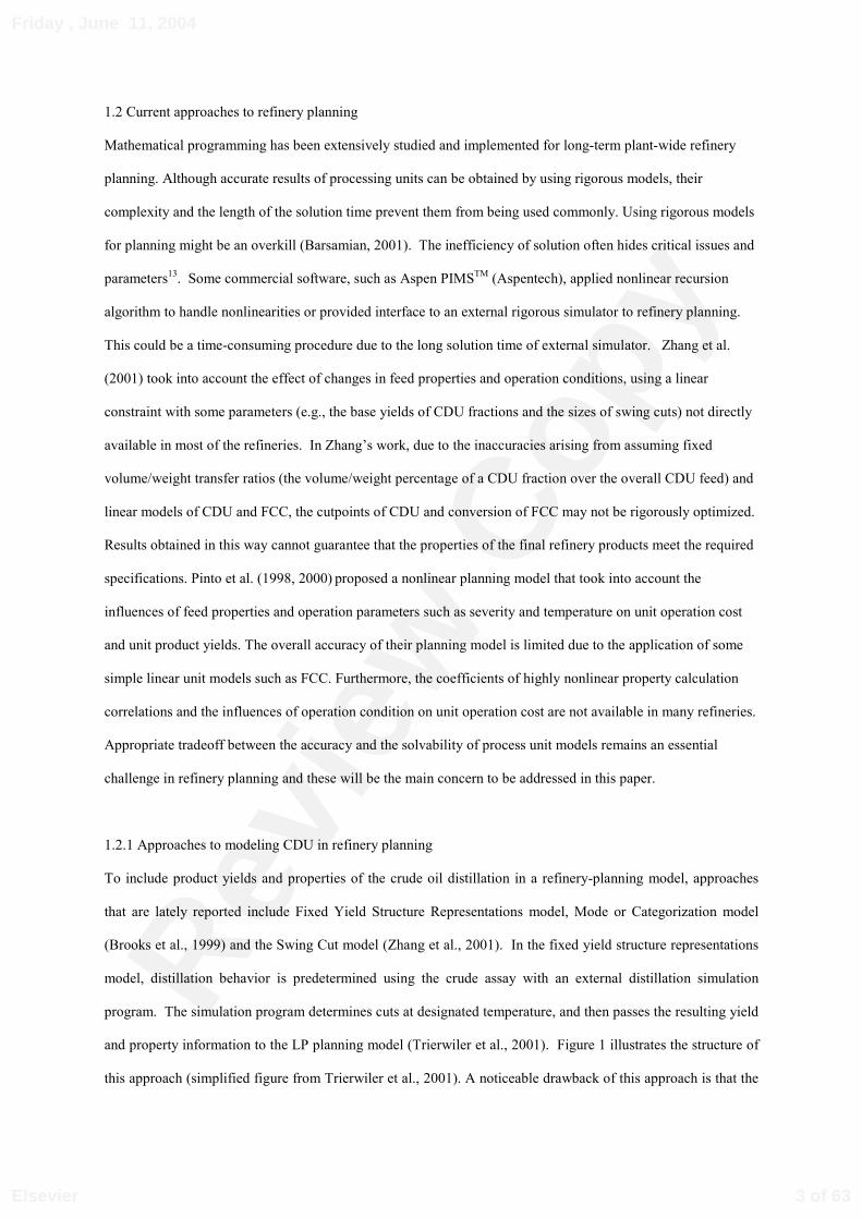
and property information to the LP planning model (Trierwiler et al., 2001). Figure 1 illustrates the structure of
this approach (simplified figure from Trierwiler et al., 2001). A noticeable drawback of this approach is that the
3 of 63
Friday , June 11, 2004
Elsevier
Revie
w C
opy
cutpoints of distillates are predetermined therefore cannot guarantee the optimality of the cutpoint settings for
CDU distillates. Some researchers (Trierwiler et al., 2001) applied a method called “Adherent Recursion” to
optimize cutpoints. The results of LP planning model (new cutpoints) were sent back to simulation software to
update the yields and properties. However, the long solution time of the simulation software running iteratively
made it a time-consuming procedure to obtain the final results.
In actual plant operation, CDU operations are often defined into several operating modes, such as gasoline mode
or diesel mode, according to the crude properties, process constraints and marketing strategies, etc. Each mode
has a set of predetermined cutpoints based upon the experience from the previous production settings. Until
now, quite a few of refineries are still using these operating modes for planning their operation due to the
simplicity of this method. In the mode or categorization approach, the LP planning model selects one of the
operation modes or the combinations of these modes to maximize the total profit. The challenge lies in how to
blend these modes effectively. Brooks et al. (1999) applied a visual approach using some figures to obtain
optimal plan by blending operating modes. They first calculated the yields and properties of CDU fractions
using rigorous CDU model. Then, taking into consideration the specifications of the final products, they used a
spreadsheet to blend CDU modes pair-wise in 1% steps. With the help of the spreadsheet, the procedure was
performed visually using some figures. However, applying their approach is rather time-consuming and, only
the yield of certain CDU fraction being maximized, the total profit maximization of a refinery is still not
guaranteed.
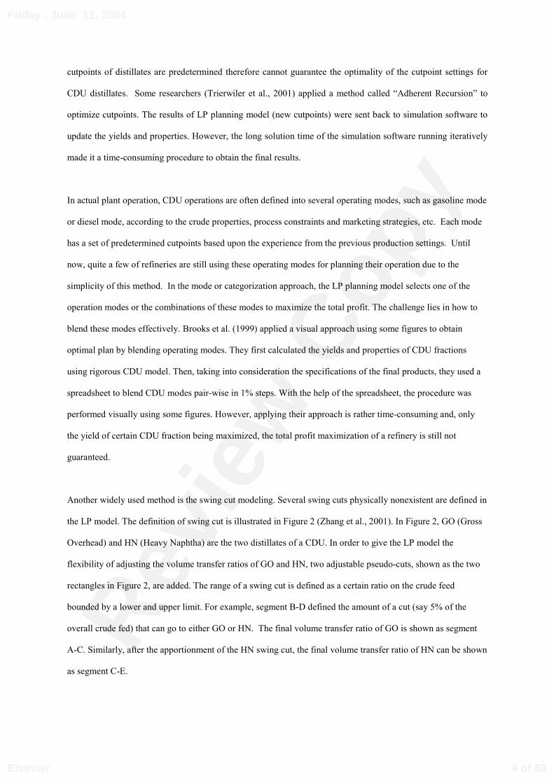
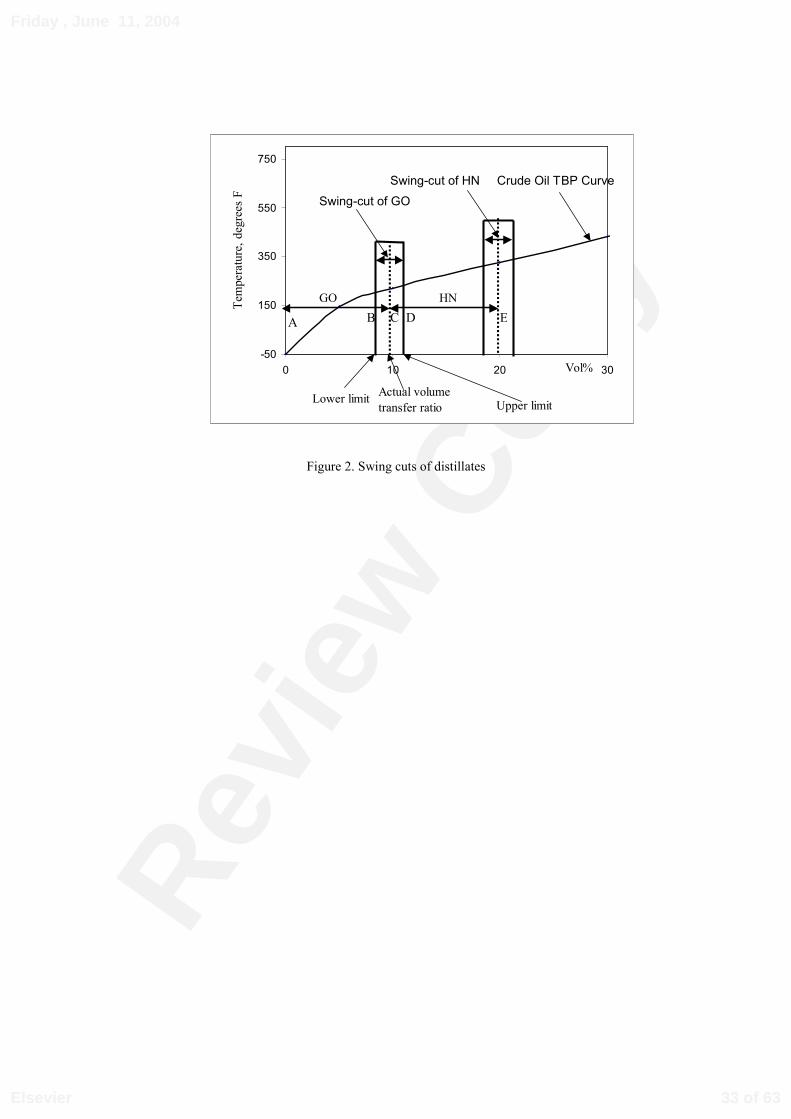
Another widely used method is the swing cut modeling. Several swing cuts physically nonexistent are defined in
the LP model. The definition of swing cut is illustrated in Figure 2 (Zhang et al., 2001). In Figure 2, GO (Gross
Overhead) and HN (Heavy Naphtha) are the two distillates of a CDU. In order to give the LP model the
flexibility of adjusting the volume transfer ratios of GO and HN, two adjustable pseudo-cuts, shown as the two
rectangles in Figure 2, are added. The range of a swing cut is defined as a certain ratio on the crude feed
bounded by a lower and upper limit. For example, segment B-D defined the amount of a cut (say 5% of the
overall crude fed) that can go to either GO or HN. The final volume transfer ratio of GO is shown as segment
A-C. Similarly, after the apportionment of the HN swing cut, the final volume transfer ratio of HN can be shown
as segment C-E.
4 of 63
Friday , June 11, 2004
Elsevier
Revie
w C
opy
Hartmann (1999) used swing cut, called “balancing cut” in his paper, to address the problem of setting cutpoints
of a CDU. The cutpoints were changed after the analysis of the marginal values of intermediate streams and
units. Zhang et al. (2001) determined the optimal flow rates of CDU fractions on the basis of fixed swing cuts.
They fixed the size of a swing cut to a certain proportion of the total feed whose value is not available directly
from a refinery.
In general, two issues need to be considered in swing cut modeling: the sizes of swing cuts and the properties of
the cut fractions. The size of a swing cut can either be expressed as certain volume transfer ratio on crude feed
or as certain boiling temperature range. Some researchers estimate the size of a swing cut by experience. Zhang
et al. (2001) used 5% and 7% volume transfer ratio on crude feed as the sizes of naphtha and kerosene swing
cuts respectively. A typical 50 degrees of boiling temperature range, can also be set to swing cuts (Trierwiler, et
al., 2001). Modelers commonly use a rather wide swing cut sizes in their initial LP run, and shorten the swing
cut sizes subsequently. This is a time-consuming procedure and also risks blocking an optimum cutpoint value
out of consideration (Trierwiler et al., 2001). Since the accurate sizes of swing cuts are unknown, some
researchers divide swing cuts into small segments in an attempt to improve modeling accuracy. Each segment is
allowed to be blended with adjacent distillates individually. While this approach may improve accuracy, the size
of the LP model grows significantly. This approach also involves applying complex mixed integer programming
to obtain reasonable results (Trierwiler et al., 2001).
In this paper, an effective method is proposed (see section 3) to determine the sizes of swing cuts. These sizes
are obtained by using the WTRs of CDU fractions, which are calculated using the empirical procedure described
by Watkins (1979) and ASTM boiling ranges for CDU fractions. Once the WTRs/swing cuts are determined, a
planning model is then used to optimize cutpoints of CDU.
The second issue is about the properties of swing cuts and fractions. Most of the research works of refinery
planning assumed that the properties of CDU fractions and the swing cut materials are constant across their
temperature ranges. However, moving a swing cut to its adjacent lighter distillate will bring heavy ends to this
lighter distillate. This will influence the properties such as octane number, pour point of the lighter distillate, and
the sulfur and cloud point that are sensitive to heavy ends. Similarly, moving a swing cut to its adjacent heavier
distillate will bring light ends to this heavier distillate, which will influence the octane number, pour point of the
5 of 63
Friday , June 11, 2004
Elsevier
Revie
w C
opy
heavier distillate, especially properties such as viscosity and flash point that are sensitive to light ends. Besides
being influenced by swing cuts, distillate properties themselves are most often highly nonlinear, and this is the
primary area where swing cut modeling fails to represent distillation behavior accurately (Trierwiler et al., 2001).
To address these problems, regression models based upon crude properties will be used to calculate the octane
numbers, pour points and API gravities of CDU distillates. Case studies are used to illustrate the importance of
the properties calculation.
In brief, the proposed refinery planning model optimizes CDU cutpoints by integrating a set of predefined
operating modes into a modified swing cut method. The predefined CDU modes are used to determine the sizes
of swing cuts (expressed as Weight Transfer Ratio Ranges (WTR) which will be defined in section 3). Beside
CDU cutpoints, the properties of CDU fractions, which are usually ignored in conventional planning models, are
calculated using the basic crude data.
1.2.2 Approaches to model FCC in refinery planning
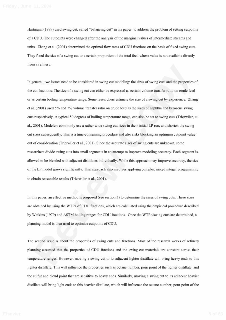
Pinto et al. (2000) used a linear model of FCC. Due to the nonlinearity of FCC behavior, a linear model of FCC
may give inaccurate yields and properties of FCC distillates. Figure 3 (Decroocq, 1984) shows a typical FCC
gasoline vs. FCC conversion level curve. The nonlinearity of this figure, especially in high conversion area, is
obvious. To accurately model FCC without introducing a too complex FCC model, a regression model based
upon the work from Gary et al. (2001) is applied in the proposed refinery planning model(section 4).
2. Problem description
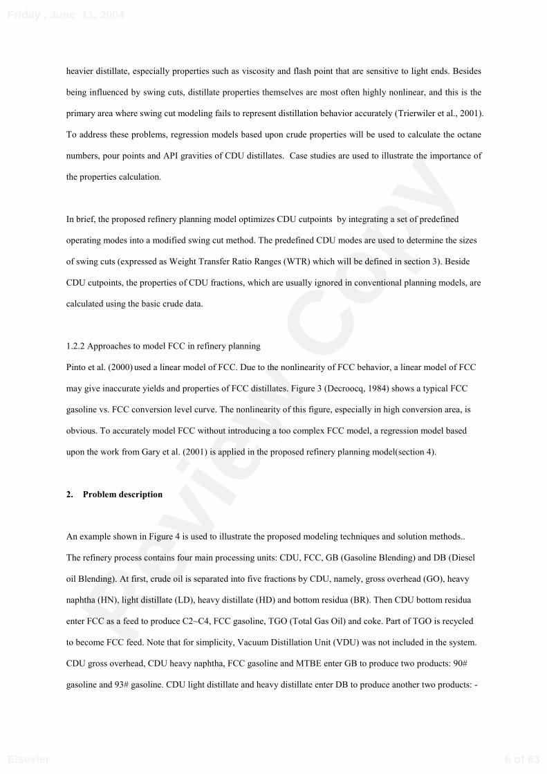
An example shown in Figure 4 is used to illustrate the proposed modeling techniques and solution methods..
The refinery process contains four main processing units: CDU, FCC, GB (Gasoline Blending) and DB (Diesel
oil Blending). At first, crude oil is separated into five fractions by CDU, namely, gross overhead (GO), heavy
naphtha (HN), light distillate (LD), heavy distillate (HD) and bottom residua (BR). Then CDU bottom residua
enter FCC as a feed to produce C2~C4, FCC gasoline, TGO (Total Gas Oil) and coke. Part of TGO is recycled
to become FCC feed. Note that for simplicity, Vacuum Distillation Unit (VDU) was not included in the system.
CDU gross overhead, CDU heavy naphtha, FCC gasoline and MTBE enter GB to produce two products: 90#
gasoline and 93# gasoline. CDU light distillate and heavy distillate enter DB to produce another two products: -
6 of 63
Friday , June 11, 2004
Elsevier

Revie
w C
opy
10# diesel oil and 0# diesel oil. C2~C4 from FCC and TGO, which is not recycled, are sold as final products.
Coke is assumed to be burned in regenerator thus valueless. The prices (yuan/ton) of raw materials and products
are shown in Table 1. The capacities of CDU and FCC are both 400 tons/day; the operation costs of CDU and
FCC are 20 and 110 yuan/ton, respectively. The market demand for each product is 200 tons/day. The octane
number of MTBE is 101. The blending requirement of gasoline blending is that the octane number of 90# and
93# gasoline products should be equal to or greater than 90 and 93, respectively. The blending requirement of
diesel oil blending is that the pour point of -10# and 0# diesel oil should be equal to or smaller than -10°C and
0°C, respectively. The objective of the problem is to maximize the total profit of the refinery by varying the
cutpoints of the CDU and conversion level of the FCC by taking into account the property changes of the
intermediate and final products.
3. Determination of the CDU Weight Transfer Ratio Ranges (WTR)
3.1. Determination of the volume transfer ratios of CDU fractions
The objective of this section is to describe the procedure of determining the flow rate range of each CDU
fraction. The ability of a refinery to meet all the specifications and conditions of final products is initially set by
the CDU fractions (Brooks et al., 1999). Thus the flow rates of CDU fractions are adjusted in a refinery all the
time to produce different quality and specification of products. However, these flow rates cannot be changed
arbitrarily, they can only be changed in their specific ranges. CDU is used to separate crude oil by distillation
into fractions according to boiling point. It is the first major processing unit in the refinery. Crude oil is a
mixture of some 100,000 liquid chemical compounds, primarily hydrocarbons ranging from methane to
extremely heavy hydrocarbon molecules with up to 80 carbon atoms. A CDU fraction is a mixture that usually
defined in terms of its ASTM (American Society for Testing Materials) boiling range. ASTM boiling range (see
Appendix A.1 for details) defines the general composition of the fraction and is usually one of the key
specifications for most distillates (Watkins, 1979). Different refineries have slightly different definitions of
ASTM boiling ranges for CDU fractions. According to the definitions of Watkins (1979), gross overhead
consists of light-ends through 250-275 °F ASTM end point; heavy naphtha consists of pentane through 400 °F
ASTM end point; light distillate has an ASTM boiling range of approximately 300-600 °F; heavy distillate has
7 of 63
Friday , June 11, 2004
Elsevier

Revie
w C
opy
an ASTM boiling range of approximately 525-675 °F. All distillates heavier than heavy distillate are called
bottom residua. Bottom residua have an ASTM end point over 1300 °F.
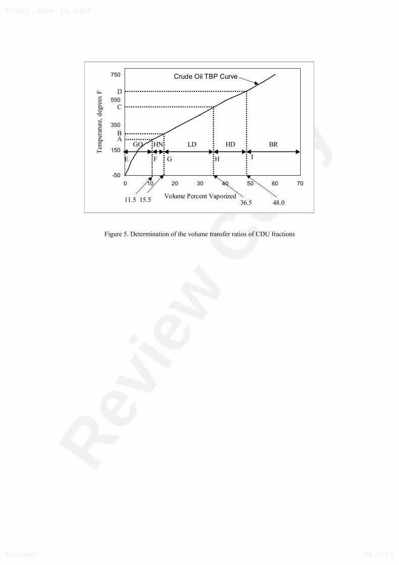
Figure 5 shows the TBP curve of a crude oil. True boiling point (TBP) distillation (see Appendix A.1 for details)
is used to analyze the component distribution of a material being tested. This method uses a distillation column
with certain number of stages and reflux so that the temperature on the curve represents the actual (true) boiling
point of the hydrocarbon material present at the corresponding volume percentage (Watkins, 1979). The
volumetric yield (also expressed as volume transfer ratio) of a CDU fraction can be obtained from the crude oil
TBP curve and its boiling point. In Figure 5, points “A”, “B”, “C” and “D” represent the cutpoints of GO, HN,
LD and HD, respectively. Draw a dotted horizontal line through each point; then draw a dotted vertical line
through the intersection of the dotted horizontal line and the crude oil TBP curve. The gap (such as segments E-
F, F-G, G-H and H-I in Figure 5) between two neighbor dotted vertical lines determines the volume transfer
ratio of a CDU fraction. In Figure 5, the volume transfer ratios of GO, HN, LD, HD and BR are 11.5, 4.0,
21.0,11.5 and 52 (=100-48.0), respectively.
3.2. Determination of operation modes
Since a CDU fraction is still a mixture of many hydrocarbons, it has a boiling range. To meet the demand for
different specifications of products from different customers or to maximize the total profit, the refinery has to
adjust the operation conditions to change the properties of CDU fractions; hence the boiling ranges of CDU
fractions vary under different operation conditions. A typical ASTM boiling range of CDU fractions is listed in
Table 2 (Watkins, 1979). The EPs (End Point, the temperature at which a distillate is 100% vaporized) and IBPs
(Initial Boiling Point, the temperature at which a distillate begins to boil) of CDU fractions provided by Watkins
(1979) are adopted in Table 2. The IBPs of HN and BR, which were not included in Watkins (1979), were
estimated here (see Appendix A.2 for details). Note that most of the refineries provide ASTM boiling ranges to
define CDU fractions, from which the boiling ranges can be adopted in Table 2.
Although ASTM boiling ranges can be easily obtained and used conveniently for product identifications, they
cannot be used directly to estimate weight transfer ratios of CDU fractions. Thus ASTM boiling ranges should
8 of 63
Friday , June 11, 2004
Elsevier
Revie
w C
opy
be converted to TBP boiling ranges. The conversion method is described in Appendix A.4. Table 3 lists the
converted TBP boiling ranges from the ASTM boiling ranges of Table 2.
Table 3 provides rough TBP ranges of the CDU fractions. For instance, if GO is the preferable product, the EP
of GO should be increased to its maximum value (290.9 °F); if HN is the preferable product, then a smaller
value (276.5 °F) is assigned to the EP of GO. With this understanding, the TBP boiling ranges of three CDU
operation modes can then be determined (Table 4). These operation modes are maximizing heavy naphtha
(M.N.), maximizing light distillate (M.L.) and maximizing heavy distillate (M.H.). The number of operation
modes defined above is relatively small and thus has a potential to reduce the size of a planning model. Note
that the three operation modes defined here are used for demonstrating the approach in this paper. Other sets of
operation modes, such as the frequently used five operation modes or the eight operation modes defined in
Brooks et al. (1999), are categorized for other CDUs according to their design and operation conditions. In fact,
the approach that we developed is independent of the number of operation modes. One can maximize the yield
of only one product on any given operation (Watkins, 1979). Thus a CDU can be at only one operation mode at
one time. A refinery can determine the operation of the CDU to be either at one of the operation modes or
somewhere among these operation modes.
3.3 Determination of Cutpoints
Due to the limitation of stage number and reflux ratio, the TBP boiling ranges of two adjacent CDU fractions
always overlap. To specify the separation temperature being used in conventional distillation columns between
two adjacent fractions, a “cutpoint” is used. It is defined as the mid-point of the TBP overlapping temperatures
(TBP cutpoint = 0.5*(EPL + IBPH), where EPL is the EP of the light fraction and IBPH is the IBP of adjacent
heavy fraction). The definition of TBP cutpoint between two fractions is shown in Figure 6 (Watkins, 1979).
The TBP cutpoint (point D) is the average temperature of the EP of light fraction (point A) and the IBP of heavy
fraction (point B). With the TBP cutpoints among fractions determined, the corresponding volume transfer
ratios of CDU fractions can then be obtained using the procedure described in Section 3.1.
3.4 Determination of VTR (Volume Transfer ratio Range)
9 of 63
Friday , June 11, 2004
Elsevier
Revie
w C
opy
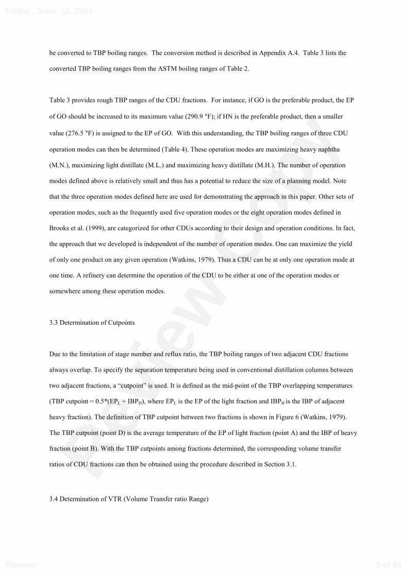
In a refinery, adjusting the cutpoints will change the volume transfer ratios (hence flow rates) and properties of
CDU fractions that affect the overall economics of the refinery. The cutpoints among CDU fractions can be
calculated using the procedure proposed in Section 3.3. These cutpoints are then used to determine VTR. The
maximum volume transfer ratio of a CDU fraction is called the upper limit of the VTR while the minimum
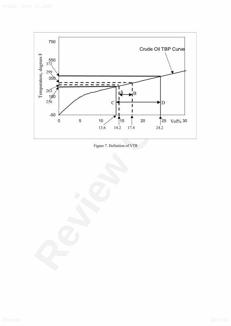
value, the lower limit of the VTR. This procedure is illustrated in Figure 7. For M.N. mode, using the data
given in Table 4, the cutpoints of HN can be calculated (256 °F for GO/HN and 372 °F for HN/LD). Then the
corresponding volume transfer ratio of HN is obtained 10.6% (=24.2%-13.6%) as shown by segment C-D.
Similarly, cutpoints in M.L. mode (263 °F for GO/HN and 299 °F for HN/LD) can be calculated, the
corresponding volume transfer ratio of HN is obtained 3.2% (= 17.4%-14.2%)) as shown by segment A-B. The
cutpoints in the M.H. mode are the same as those in the M.L. mode in this case, thus the volume transfer ratio of
HN in M.H. mode is the same. The upper limit of the VTR of HN is then 10.6% and the lower limit is 3.2%.
Thus the VTR of HN is (3.2%, 10.6%).
In a refinery, flow rates of CDU fractions are often based on weight. It is more convenient to express the ratios
of CDU fractions as weight transfer ratios. The volume transfer ratio in crude oil TBP curve should then be
converted to weight transfer ratio and the VTRs become WTRs. To perform this conversion, the API gravity
( 5.131141.5/d gravity API 15.615.6 −= , where 6.15
6.15d is the specific density at 60 °F) has to be used. This API gravity
is usually included in a crude assay. As an illustration, the crude assay data from Watkins (1979) are used here
to calculate the API gravity of crude oil and CDU fractions (see Appendix A.3 for details). For the example
illustrated in Figure 7, the corresponding WTR is (2.8%, 9.5%).
The VTR/WTR focuses on the transfer ratio range of a fraction while the commonly used swing cut is a pseudo-
cut that exists between two fractions. The sizes of swing cuts can be determined with the knowledge of
VTR/WTR, and vice versa. For the example illustrated in Figure 7, the size of the swing cut (if expressed as
volume ratio on crude feed) between GO and HN is 0.6% (= 14.2% – 13.6%) which is small and the size of the
swing cut between HN and LD is 6.8% (= 24.2% - 17.4%) which is rather large. The accurate sizes of swing
cuts can thus be determined by the procedure proposed in this paper. For easy integration of the CDU model
with the main planning model, VTR/WTR is used in this paper.
3.5. WTR determination procedure
10 of 63
Friday , June 11, 2004
Elsevier
Revie
w C
opy
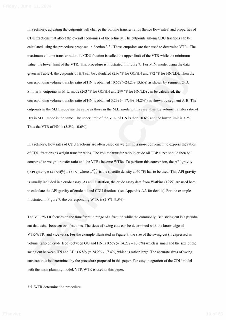
The procedure described in Sections 3.1 to 3.4 for determining the WTR of CDU fractions is summarized in this
section and illustrated in Figure 8. The manual procedure described by Watkins (1979), the accuracy of which is
tested by rigorous simulation in Appendix B.1, is used for computer calculation. The procedure uses ASTM
boiling ranges of CDU fractions and crude assay data available in most refineries. The detailed procedure
consists of four major steps as follows.
Step 1. The determination of ASTM D86 boiling ranges and operation modes
The ASTM boiling ranges of CDU fractions can be obtained from refineries, CDU designers or from literatures
(e.g., Watkins, 1979, Gary et al., 2001). These ASTM boiling ranges are used as the starting point of the
procedure proposed here. The ASTM boiling ranges used in this paper are listed in Table 2. These ASTM
boiling ranges are converted to TBP boiling ranges using the correlations developed by Watkins (1979) (see
Appendix A.4 for details). Other correlations (Arnold, 1985) for ASTM to TBP boiling range conversion can
also be used according to their accuracies for different crude oils. The converted TBP boiling ranges are listed in
Table 3 and the TBP boiling ranges of the three operation modes are then determined and listed in Table 4.
Step 2. Calculate the cutpoints for operation modes
The cutpoints for operation modes are calculated using the method described in Section 3.3. For example, to
calculate the cutpoint between GO and HN in the M.N. mode, we know from Table 4 that EPL is 276.5 °F and
IBPH is 235.4 °F, therefore the cutpoint of GO/HN is (276.5+235.4)*0.5 = 255.9 °F. The calculated cutpoints are
listed in Table 5.
Step 3. Calculate CDU fractions weight transfer ratios for the operation modes
The crude oil TBP data and CDU fractions API data from crude assay are correlated to form the crude oil TBP
equation and CDU fractions API equations (See Appendix A.3 for details). The calculated cutpoints for
operation modes (Table 5) are then sent to crude oil TBP equation to calculate the volume transfer ratios of
CDU fractions. For example, the cutpoint for GO/HN in the M.N. mode (255.9 °F) is sent to crude oil TBP
equation and then the volume transfer ratio of GO (13.61) in this mode can be obtained. The API gravity of each
fraction is calculated by inserting its volume transfer ratio into its API gravity equation. Using this calculated
API gravity, the volume transfer ratio of a CDU fraction is then converted to weight transfer ratio. The above
11 of 63
Friday , June 11, 2004
Elsevier

Revie
w C
opy
procedure is performed for each operation mode to obtain the weight transfer ratios of CDU fractions in each
mode. The calculated API gravities of CDU fractions are listed in the last column of Table 6. The calculated
weight transfer ratios and volume transfer ratios for each operation mode are listed in the second last and the
third last columns of Table 6, respectively.
Step 4. Determination of WTR
After the weight transfer ratios corresponding to the operation modes obtained in Step 3, the maximum and
minimum weight transfer ratios are selected from the modes for each CDU fraction. The maximum and
minimum volume and weight transfer ratios are listed in the third and fourth columns of Table 6, respectively.
For example, the number 11.73 in the fourth column is the maximum value of the three numbers (11.17, 11.72,
11.73) in the second last column; the number 11.17 in the fourth column is the minimum value of the three
numbers (11.17, 11.72, 11.73) in the second last column. These maximum and minimum weight transfer ratios
are then sent to the main planning model as WTRs to optimize the cutpoints of CDU fractions. It is assumed that
the crude oil is Tia Juana Light and the crude assay data from Watkins (1979) are used in this paper. The
calculated WTRs are also compared with results of rigorous simulation in Appendix B.2.
4. Model for FCC fractions transfer ratios
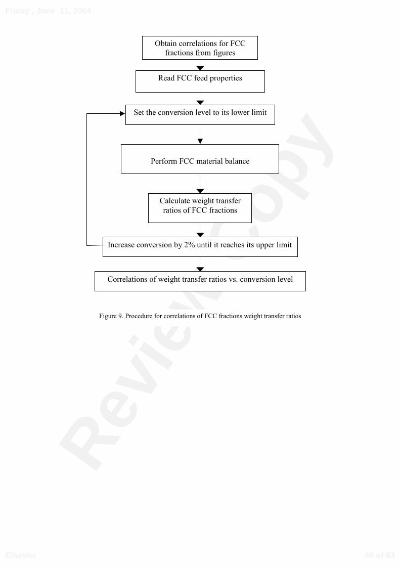
4.1 Description of the procedure
A procedure for the determination of FCC fractions’ weight transfer ratios (the weight percentage of a FCC
fraction over the overall FCC feed) as a function of FCC conversion is proposed in this section. The major
operating variables affecting the FCC conversion level are the cracking temperature, catalyst/oil ratio, space
velocity, etc. The hand-calculation procedure described by Gary et al. (2001) is implemented in our proposed
procedure. The procedure is illustrated in Figure 9. Firstly, we obtained FCC fractions yield correlations (when
zeolite catalyst is used in FCC) from figures provided by Gary et al. (2001) (see Appendix C for details). Then
the feed properties, API gravity and Watson characterization factor were read. The lower limit and upper limit
of FCC conversion are determined according to FCC operation conditions such as the regenerator coke burning
ability. The conversion range used in this paper is (60%, 85%). This is followed up by a sequence of actions: Set
the conversion level to its lower limit (60%), perform FCC material balance according to the procedure
12 of 63
Friday , June 11, 2004
Elsevier

Revie
w C
opy
described by Gary et al. (2001), and calculate the weight transfer ratios of FCC fractions. Next, there is the need
to increase the conversion by a small value (2%) and calculate the weight transfer ratios corresponding to the
current conversion level until the conversion level reaches its upper limit (85%). Finally, using the data obtained
above, FCC fractions weight transfer ratios and FCC conversion level are correlated. An equation of each FCC
fraction weight transfer ratio vs. FCC conversion level is now obtained and can be used in refinery planning
model to optimize the FCC conversion level. Table 7 lists the correlations for FCC fractions (the feed properties
is assumed to be: Watson characterization factor =11.8, API=19). In Table 7, “WT” represents the weight
transfer ratio of C2~C4 or FCC gasoline, etc. “Conv” represents the conversion level of FCC. For different feed
properties of FCC, one can apply the same procedure described above to obtain the same type of correlations
with different parameters.
4.2 Discussion of the procedure
The discrepancy between the correlations obtained above and the figures provided by Gary et al. (2001) is about
1~3%, which is within the accuracy of those figures. The procedure is much simpler and faster compared with a
rigorous FCC model. The required input (API gravity and characterization factor of the feed) can also be easily
obtained from refineries. The emphasis of the FCC model proposed in this paper was put on its solution speed
and the effectiveness so that it can be integrated into the main planning model directly. Since the input-output
relationship of FCC can be updated by some online learning methods or through the improvement of relevant
technologies, the FCC model can be readily updated with higher accuracy.
Further improvement for this procedure can be made by:
• Updating the figures provided by Gary et al. (2001). It is pointed out (Magee et al., 1993) that as the
improvement of catalysts and unit design, the yield data of FCC fractions will change and hence
corresponding figures should be updated. Besides, the yield of gasoline vs. conversion keeps increasing in
the figure provided in Gary et al. (2001). In reality, the yield of gasoline will decrease as the conversion
increases to a certain value.
13 of 63
Friday , June 11, 2004
Elsevier
Revie
w C
opy
• It is assumed in this paper that the feed properties of FCC feed remain constant. However, the physical
properties of the feed will change as the recycle stock or the CDU operation conditions change. This should
be considered in future works.
5. Product Blending
Blending is a very important and complicated issue in refinery planning. As a demonstration, two commonly
used blending models are described in this section. However, the whole modeling concept is not limited to these
two blending models which can be replaced by other state-of-the-art models.
5.1 Blending rule
Some quality indicators, such as octane number and freezing point, are used to prove whether or not the gasoline
meets the quality specifications. In the case of diesel oil, pour point, cetane number and viscosity, among others,
are used as key quality indicators. In this paper, octane number (ON) and pour point (PP) are used as the quality
index of gasoline and diesel oil, respectively.
• Gasoline blending
In gasoline blending, the octane number of a blended product can be simply calculated using the following
linear equations:
ppii f*Of*O =∑
ff pi =∑
where iO is the octane number of intermediate stream i; if is the flow rate of the intermediate stream i; pO is
the octane number of product p; pf is the sum of if .
• Diesel oil blending
For diesel blending, diesel properties such as pour point cannot be calculated using a simple linear equation.
Some correlations have been proposed for diesel oil blending. Reid and Allen (1951) used linear combination of
pour point blending indexes of intermediate streams to predict product pour points. Hu and Burn (1970)
proposed a nonlinear one-parameter pour point equation. Semwal et al. (1995) proposed an improved nonlinear
correlation which is used in this paper:
)(T*)(V1
iA
i∑=
=n
i
BBbT
where bT is the pour point of product, Vi and Ti are volume fraction and pour point (in the Rankine degree, °R)
of intermediate stream i, respectively. Four sets of parameters “A” and “B” are given in different pour point
14 of 63
Friday , June 11, 2004
Elsevier

Revie
w C
opy
ranges. The wide pour point range (from –21 to 51 °C) is used in this paper. The corresponding values of A and
B are 1.105 and 12.987, respectively.
5.2 Calculation of the properties of CDU fractions
The octane numbers or pour points of CDU fractions will change as the cutpoints of CDU change. In our
planning model, the octane numbers or pour points of CDU fractions are correlated to their mid-point weight
transfer ratios. The relationship between mid-point volume transfer ratio (Mid_VTR) and octane number/pour
point are given by Watkins (1979). In this paper, mid-point weight transfer ratio (Mid_WTR) is used instead of
Mid_VTR for consistence. The equations for relating mid-point weight transfer ratios and octane numbers/pour
points from the crude assay data provided by Watkins (1979) are given in Table 8. In Table 8, the outputs of
row “GO” and “HN” are octane numbers (ON) while the outputs of row “LD” and “HD” are pour points (PP).
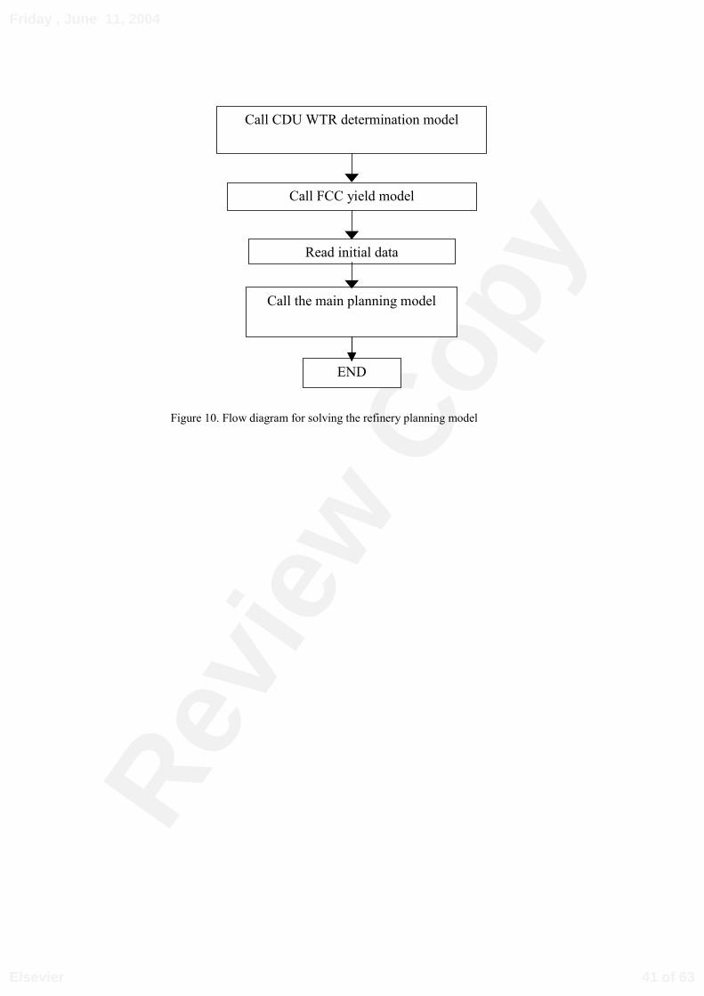
6. Main flow diagram for solving the refinery planning model
The main flow diagram for solving the refinery planning model is illustrated in Figure 10. The whole procedure
consists of the following steps:
• Call CDU WTR determination model to calculate the maximum and minimum weight transfer ratios of
CDU fractions.
• Call FCC yield model to obtain equations of FCC fraction weight transfer ratio vs. FCC conversion. These
equations are used in the refinery model.
• Read initial data, which include the data of unit capacities, unit operation costs, initial octane numbers and
pour points and CDU WTRs.
• Integrate the CDU and FCC models with the main NLP planning model and solve the main model.
Compare to the rigorous CDU and FCC models, the solution time of the two CDU and FCC models proposed
here was reduced significantly. In most of the cases tested in this study, the CPU time needed to solve the main
planning model is 0.1 to 0.2 second.
7. Case studies
15 of 63
Friday , June 11, 2004
Elsevier
Revie
w C
opy
Several case studies demonstrate the effectiveness of the CDU and FCC models proposed in this paper. The
refinery planning model is formulated in GAMS (Brooke et al., 1992) on a 933MHz Pentium III PC. The code
MINOS5 in GAMS 2.25 is used for NLP. The planning model is described in Appendix D.
The configuration of the cases studied here is illustrated in Figure 4. The price data for these cases are listed in
Table 1. The unit capacities, operation costs, market demands for products and blending requirements for
blending units are described in Section 2. The influences of different CDU cutpoint setting methods on total
profit will be studied in Section 7.1 while the influences of different FCC conversion level determination
methods on total profit and FCC fractions weight transfer ratios will be studied in Section 7.2. Finally Section
7.3 studies the influences of different methods of determining CDU fractions’ properties on total profit and the
weight transfer ratios of CDU fractions.
7.1 CDU cutpoints determination
Up to now, many refineries still use one of the operation modes, such as M.N., M.L. or M.H., as their CDU
operation condition, whose cutpoint setting of CDU fractions is not optimal. Different cutpoint setting methods
are compared here (The FCC conversion level and CDU fractions’ properties in these cases can be varied by the
planning model). Firstly, a refinery may fix the weight transfer ratios of CDU fractions at either M.N., M.L. or
M.H. mode. (The fixed weight transfer ratios of these modes are listed in Table 9). The corresponding solution
results are listed in the second to fourth rows of Table 10. The optimal solution (in which the weight transfer
ratios of CDU fractions are optimized) obtained by solving the planning model proposed in this paper, is listed
in the first row. It can be seen that the optimal cutpoint setting is located somewhere among the operation
modes. If the cutpoint’s setting is fixed for M.N., the profit will decrease by 24.5%. After the determination of
CDU WTRs from the proposed procedure and the data obtained from refineries, the optimal cutpoint can be
calculated by solving the planning model. A refinery should not set the CDU cutpoints according to any of the
operation modes arbitrarily. The optimal cutpoint should be obtained by solving the planning model with the
consideration of factors such as current market prices of raw materials and products, unit operation costs, and
processing constraints, etc. The results of this case study are mainly consistent with those of Brooks et al. (1999)
with total profit maximized and simpler procedure.
16 of 63
Friday , June 11, 2004
Elsevier

Revie
w C
opy
7.2 FCC conversion optimization
The FCC severity (expressed as conversion level) is a very important parameter in a refinery. Similar to the
setting of the cutpoints, the optimal FCC conversion should also be decided according to the current situation.
Two cases are studied in this section (The CDU fractions’ weight transfer ratios and properties can be varied
and optimized). The FCC conversion is fixed at 65.0% in the first case while the FCC conversion level is
calculated and optimized in the planning model in the second case. The results are listed in Table 11. It can be
seen from the table that the total profit of the fixed conversion level case decreased by 2.1% compared to the
optimal conversion (73.4%) case. A refinery should then adjust the FCC operation conditions, such as reaction
temperature or catalyst/oil ratio, to change the conversion to the optimal value.
7.3 Physical properties calculation
Most of the research works of refinery planning still assumed that the properties of CDU fractions are constant.
However, following the change of the cutpoints, the properties of fractions will also change. From Appendix
B.3, it can be seen that the octane numbers of CDU fractions change several units in different situations. Table
12 lists the comparison of different calculation methods of properties (The CDU weight transfer ratios and FCC
conversion level can be varied by the planning model). In the first row, the octane numbers and pour points are
calculated whenever the cutpoint settings are changed while the octane numbers and pour points are estimated
and fixed in the second and the third rows. After the planning model is solved (the first row), the final properties
can be obtained. For example, it is found that the final octane number of CDU gross overhead is 60.9. This
value can be used in gasoline blending to calculate the yield of final gasoline products. If the properties are
estimated and fixed to certain values, for example, the octane numbers of GO and HN are fixed to 50.0 and 65.0
respectively and the pour points of LD and HD to –40.0 and 5.0 degree C respectively, then the total profit may
be underestimated (the second row) or overestimated (the third row) and the corresponding CDU cutpoint
setting and product yields will also be influenced. The reason is that the product quality in the second row was
underestimated (The real octane number of 90# gasoline is 92.7) while the product quality in the third row was
overestimated (The real octane number of 90# gasoline is 88.3). The refinery may lose the potential of earning
more money (the second row) or risk the products refused by customers (the third row). Thus it is important to
calculate the properties of CDU fractions using some correlations.
17 of 63
Friday , June 11, 2004
Elsevier

Revie
w C
opy
8 Conclusions
In this paper, the optimal planning strategies of refineries are studied and a procedure for the CDU WTRs
determination is proposed. A yield model is used for the determination of equations of FCC fractions’ weight
transfer ratios vs. FCC conversion level. With the CDU and FCC models integrated into the planning model, the
CDU cutpoints and FCC conversion level can be optimized accurately. The properties of CDU fractions are
calculated in the model to reflect the influence of CDU cutpoints’ changes that guarantee the quality of the final
products. Finally, several case studies are described and solved using the proposed planning model to illustrate
the significance of the CDU and FCC models and the calculation of CDU fractions’ properties.
Acknowledgments
The authors would like to acknowledge financial support from the Research Grant Council of Hong Kong
(Grant No. HKUST6014/99P & DAG00/01.EG05), the National Science Foundation of China (Grant No.
79931000) and the Major State Basic Research Development Program (G2000026308).
18 of 63
Friday , June 11, 2004
Elsevier

Revie
w C
opy
References
Arnold, V. E. (1985) Microcomputer program converts TBP, ASTM, EFV distillation curves, Oil & Gas Journal. 83(6) Feb 11, 55-62
ASPEN PLUS, version 11.1; Aspen Technology, Inc. : Cambridge, MA, 2001
Barsamian, A. (2001) Fundamentals of Supply Chain Management for Refining, IBC Asia Oil &Gas SCM Conference Proceedings, April
26, Singapore
Blanding, F. H. (1953) Reaction rates in Catalytic Cracking of Petroleum, Industrial & Engineering Chemistry, 45(6), 1186~1197
Brooke, A., Kendrick, D. & Meeraus, A. (1992) GAMS — A User’s Guide (Release 2.25); San Francisco, CA: The Scientific Press.
Brooks, R.W. et al. (1999) Choosing cutpoints to optimize product yields, Hydrocarbon Processing, November, 53-60
Cechetti, R.C. et al. (1963) Hydrocarbon Processing, 42(9), 159
Decroocq, D., (1984) Catalytic Cracking of Heavy Petroleum Fractions, Editions Technip.
Gary, J. H., & Handwerk, G. E. (2001) Petroleum Refining Technology and Economics, 4th Ed., Marcel Dekker
Hartmann, J.C.M. (1999) Interpreting LP outputs, Hydrocarbon Processing, February, 64-68
Hartmann, J.C.M. (2001) Determine the optimum crude intake level—a case history, Hydrocarbon Processing, June, 77-84
Hess, F.E. et al. (1977) Hydrocarbon Processing, 56(6), 181
Hu, J., & Burns, A.M. (1970) New Method Predicts Cloud, Four Flash Points of Distillate Blends, Hydrocarbon Processing, 49(11), 213-16
Jacob, J.S., Gross, B., Voltz, S.E. & Weekman, V.W. (1976) A lumping and reaction scheme for catalytic cracking, AIChE J., 22(4),
701~713
Lang, P., et al. (1991) Modelling of a crude distillation column, Computers and Chemical Engineering, 15(2), 133-139
Magee, J.S., Maurice, M. & Mitchell, J. (1993) Fluid catalytic cracking: science and technology, Amsterdam : Elsevier
Nelson, W.L. (1958) Petroleum Refinery Engineering, 4th Ed., McGraw-Hill Book Co., Inc.
Packie, J.W. (1941) Distillation equipment in the oil-refining industry, AIChE Transactions, 37, 51-78
Perry, R. H., Green, D. W., & Maloney, J. O. (1997). Perry’s chemical engineers’ handbook (7th ed.). New York: McGraw-Hill.
Pinto J.M., Joly M. & Moro L.F.L (2000) Planning and scheduling models for refinery operations, Computers and Chemical Engineering, 24
(9-10), 2259-2276.
Reid, E.B., & Allen, H.L. (1951) Estimating Pour Points of Petroleum Dist. Blends, Petroleum Refiner, 30 (5), 93-95
Russell, R.A. (1983) A flexible and reliable method solves single-tower and crude-distillation-column problems, Chem. Engng., Oct 17, 53-
59
Semwal, P.B. & Varshney, R.G. (1995) Predictions of pour, cloud and cold filter plugging point for future diesel fuels with application to
diesel blending models, Fuel 74(3), 437-444
Trierwiler, D. & Tan, R.L. (2001) Advances in crude oil LP modeling, Hydrocarbon Asia, November/December, 11(8), 52-58
Watkins, R.N. (1979) Petroleum Refinery Distillation, 2nd Ed., Gulf Publishing Co., Houston
Zhang, J., Zhu, X.X. & Towler, G.P. (2001) A Level-by-Level Debottlenecking Approach in Refinery Operation, Industrial and
Engineering Chemical Research 40(6), 1528-1540
19 of 63
Friday , June 11, 2004
Elsevier

Revie
w C
opy
Appendix A
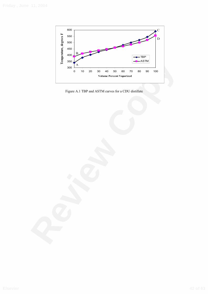
A.1 Definition of ASTM and TBP curves
True boiling point (TBP) is run in columns with 15 or more theoretical plates, which provides a very accurate
component distribution for the material being tested. However, due to the large sample size and time
requirement, TBP tests are generally only run on crude oil streams. The ASTM D86 test, which is the
standardized method established by the American Society for Testing Materials, is a batch laboratory distillation
involving approximately one equilibrium stage and no reflux. ASTM D86 test is mainly applied for products
and petroleum fractions such as CDU fractions. Typical TBP and ASTM curves of a CDU fraction are shown in
Figure A.1. Points A and B in Figure A.1 are the initial boiling points (IBP) of TBP and ASTM curves of a
CDU distillate, respectively. IBP is the temperature at which a distillate begins to boil. Points C and D in Figure
A.1 are the end points (EP) of TBP and ASTM curves of a CDU distillate. EP is the temperature at which a
distillate is 100% vaporized. Even though the ASTM tests are the simplest and most common distillations
performed on petroleum fractions, they do not provide the type of information given in TBP distillations
necessary for prediction of operating conditions or equipment design. Thus the ASTM data of petroleum
fractions need to be converted to TBP data using some correlations.
A.2 Estimation of the IBPs of HN and BR
The IBPs of HN are estimated in this paper with the consideration of the ASTM (5-95) Gap between GO and
HN. The ASTM (5-95) Gap defines the relative degree of separation between adjacent fractions. It is determined
by subtracting the 95 volume percent ASTM temperature of a fraction from the 5 volume percent ASTM
temperature of the adjacent heavy fraction (Watkins, 1979). The ASTM (5-95) Gap between GO and HN
recommended by Watkins (1979) is +20 to +30 °F. The IBPs of BR are estimated using a trial-and-error method
with the consideration of the TBP overlap between HD and BR. TBP overlap is determined by subtracting the
TBP EP of a fraction from the TBP IBP of the adjacent heavy fraction (TBP overlap = EPL- IBPH). A TBP
overlap of 80 to 100 °F between HD and BR is recommended by Watkins (1979).
A.3 Correlations of crude oil TBP curve and API gravity
20 of 63
Friday , June 11, 2004
Elsevier
Revie
w C
opy
The crude oil TBP data and CDU fractions API data from crude assay provided by Watkins (1979) are
correlated using LSM to form the crude oil TBP equation (Equation (A.1)) and CDU fractions API equations
(Equations (A.2) and (A.3)). The volume transfer ratios of CDU fractions can be calculated by inserting
cutpoints into Equation (A.1). Equation (A.2) is obtained after correlating the API gravity data of CDU fractions
(except BR) from crude assay data. The API gravity of BR is correlated into Equation (A.3). The API gravity of
each fraction can be calculated by inserting the volume transfer ratio of each fraction into Equation (A.2) or
(A.3). Note that in Equation (A.2), the API gravity is correlated to the mid-point volume transfer ratios. The
definition of a mid-point volume transfer ratio is shown in Figure A.2. The mid-point volume transfer ratio of a
CDU fraction is half of its volume transfer ratio plus the sum of the volume transfer ratios of fractions that are
lighter than it. For example, in Figure A.2, D is the mid-point of segment A-B, E is the mid-point of segment B-
C, then the mid-point volume transfer ratio of GO is shown by segment A-D and the mid-point volume transfer
ratio of HN is shown by segment A-E (= “A-B” + “B-E”).
∑=
=6
0
iz)-(TBP_CP*aVOL i
i
(A.1)
where: VOL, percent volume transfer ratios; TBP_CP, TBP cutpoint temperature;
a0, 31.25; a1, 0.09775; a2, 3.22E-06; a3, -7.646E-08; a4, 1.1817E-10; a5, -2.28E-14;
a6: -1.366E-16; z: 444.25
∑=
=8
0
iz)-(Mid_Vol*aAPI i
i(A.2)
where: API, API gravity of the CDU fraction (except BR);
Mid_Vol, Mid-volume transfer ratio of the CDU fraction;
a0, 35.4666; a1, -0.476; a2, -0.0034; a3, -0.0005855; a4, 0.0000291;
a5, 1.02E-06; a6: -3.7E-08; a7: -5.4E-10; a8: 1.6E-11; z: 41.97
∑=
=2
0
iz)-(Vol*aBR_API i
i(A.3)
where: BR_API, Bottom residua API gravity; Vol, percent volume transfer ratio of BR;
a0, 15.552; a1, 0.2932; a2, -0.00199; z, 41.6875
A.4 Conversion of ASTM boiling ranges to TBP boiling ranges
21 of 63
Friday , June 11, 2004
Elsevier
Revie
w C
opy
The ASTM boiling ranges are converted to TBP boiling ranges using the correlation proposed by Watkins
(1979). The figure for the relationships between ASTM and TBP initial and final boiling points provided by
Watkins (1979) are correlated in this paper to form Equations (A.4) and (A.5). The ASTM IBPs are converted to
TBP IBPs using Equation (A.4) while the ASTM EPs are converted to TBP EPs using Equation (A.5).
∑=
=4
0
iz)-(ASTM_IBP*aTBP_IBP i
i(A.4)
where: TBP_IBP, calculated TBP IBP; ASTM_IBP, ASTM IBP;
a0, 522.458; a1, 1.1274; a2, -8.27E-05; a3, -8.19E-07; a4, 3.336E-09; z: 555.0
∑=
=4
0
iz)-(ASTM_EP*aTBP_EP i
i(A.5)
where: TBP_EP, calculated TBP EP; ASTM_EP, ASTM EP;
a0, 547.783; a1, 1.06536; a2, -8.53E-06; a3, -8.5E-08; a4, 1.41E-09; z: 521.769
Appendix B: Comparison with Rigorous CDU Simulation Results
Part of the manual method described by Watkins (1979) is transformed for computer calculation and applied for
WTRs determination in this paper (described in section 3.5). In this appendix, the accuracies of the Watkins’
method, the WTRs determination procedure and the fractions’ property calculation are tested by rigorous CDU
simulation using Aspen Plus® version 11.1 (Aspentech, 2001). The configuration of the CDU is the same as
example 2.5 in Watkins (1979). The CDU has 29 stages in which the condenser is the first stage. Crude oil was
fed at stage 26. There exist three sidestrippers which draw oils from the main column at stages 7, 15 and 21,
respectively. Each sidestripper has 4 stages. The flow rates of the stripping steams of the main column and
sidestrippers 1# to 3# are 12,000 Ib/hr, 4,292 Ib/hr, 7,250 Ib/hr and 4,167 Ib/hr, respectively. No pumparound
exists in this example. The condenser and the bottom stage pressures are 27.8 and 38.5 psi, respectively. The
furnace overflash is 2.0 volume percent of crude feed.
The crude feed has a flow rate of 100,000 bbl/day, a temperature 200 °F and pressure 60 psi. The crude oil is Tia
Juana Light and the crude assay data (including the TBP curve, light ends composition and the API gravity
curve) from Watkins (1979) are used. The simulation is carried out with pseudocomponents spaced at 8 °F in the
range 100-800 °F and 10 °F in the range 800-1640 °F.
B.1 Comparison of the Watkins’ CDU calculation results
22 of 63
Friday , June 11, 2004
Elsevier
Revie
w C
opy
The end point settings of CDU fractions used in the Aspen Plus simulation are listed in the first row of Table
B.1. Note that the EP of HD is changed to 740 °F because the EPs of heavy fractions (HD and BR) calculated by
Aspen Plus are higher due to different property calculation methods used by Aspen Plus and Watkins. Table B.2
shows the Aspen Plus simulation results and the results calculated by Watkins. In Table B.2, it can be seen that
the difference of the mass balance between the two methods is rather small. For heat balance, as one of the
figures showing the accuracy, the calculated heat duty of the condenser by Watkins is 205.147 MMBTU/hr
while by Aspen Plus is 203.914 MMBTU/hr, where the difference is 0.6%.
The method by transforming the Watkins manual procedure to computer calculation is much faster than the
Aspen Plus simulation. The CDU mass balance by the method described in section 3.5 can be finished in 1
second while the Aspen Plus CDU simulation model needs around 30 to 190 seconds to obtain the results.
Another drawback of Aspen Plus CDU simulation model is its instability. We found that Aspen Plus CDU
simulation model sometimes gives us significantly different results even though we only reinitialize the
calculation without any changes or we change the value of a parameter a bit. It thus brings oscillations into main
planning model when incorporating Aspen Plus CDU simulation model into a commercial software such as
Aspen PIMSTM (Aspentech). We conclude that the method described in section 3.5 has higher accuracy than the
traditional linear CDU models and better solution speed than a rigorous simulation model.
B.2 Comparison of WTRs
The Aspen Plus CDU simulation model is used to calculate the WTRs by setting the end points of CDU
fractions at three operation modes (rows 2 to 4 in Table B.1). The IBPs of CDU fractions are ignored for easy
convergence. The weight transfer ratios of CDU fractions calculated by Aspen Plus CDU simulation model and
method used in this paper are listed in Table B.3. The calculated WTRs of CDU fractions are listed in Table B.4.
In Table B.3 and B.4, it can be seen that the difference of the results between the two methods is rather small.
The differences may originate from different correlations used for property calculation and CDU mass balance
and other unknown parameters such as the Murphree efficiencies of stages. In the Watkins’ manual calculation,
some correlations were read from graphs which may bring inaccuracies. For example, a curve for converting
ASTM initial boiling points to TBP initial boiling points (see Appendix A.4 for details) was used. With updated
correlations, the accuracy of the calculation can be readily improved.
23 of 63
Friday , June 11, 2004
Elsevier

Revie
w C
opy
B.3 Comparison of property calculation
As the change of the weight transfer ratios of CDU fractions, the properties of CDU fractions will also change.
Table B.5 lists the calculated octane numbers of GO and HN corresponding to the maximal and minimal weight
transfer ratios. Note that due to the nonlinearity of the property calculation, the maximal and minimal values of
CDU fractions’ properties may not happen when the weight transfer ratios take their maximal or minimal values.
It can be seen that the octane numbers of CDU fractions change several units in different situations. Assuming
fixed octane numbers of CDU fractions may not guarantee the quality of final products and may obtain sub-
optimal planning results. Similar results can be obtained for pour points calculation of CDU fractions.
Appendix C: Correlations of FCC fractions weight transfer ratios
Relevant figures provided by Gary et al. (2001) are correlated using LSM for computer calculation (Tables B.1
and B.2). As the results in Table C.1 show, the equation ∑∑= =
−− −−=3
1
2
1
11 )(*)(*i j
jiij yyxxaz should be used to
calculate the weight or volume transfer ratios of FCC fractions or the API gravity of FCC fractions. In column
“z”, “WT%” means the output is weight transfer ratio; “VOL%” means the output is volume transfer ratio and
“API” means the output is API gravity. Columns x and y show the two input variables. In x, “Conv” is the FCC
conversion level (in percentage); in y, K is the Watson characterization factor of FCC feed and API is the API
gravity of FCC feed. Note that Fuel Gas, C3=, C4=, i-C4, and n-C4 in Table C.1 are aggregated into one FCC
fraction “C2~C4” (Figure 4) in our planning model, TGO is the aggregate of HGO and LGO. Table C.2 shows
the correlated result of C3. The equation used for Table C.2 is )^2x-(conv*a2)x-(conv*a1a0Vol ++= ,
where “Vol” is the volume transfer ration of C3, “Conv” is the conversion level of FCC.
Appendix D: Definitions and mathematical formulations of the main planning model
C.1. Definitions of Indices and Parameters
(a) Indices
u = different units in the refinery, represents CDU and FCC
24 of 63
Friday , June 11, 2004
Elsevier
Revie
w C
opy
p = different types of products, represents 90#, 93# gasoline, -10#, 0# diesel oil, FCC C2~C4 and FCC heavy oil,
respectively
s,ss = different fractions from CDU, represents GO, HN, LD, HD and BR, respectively
t = different fractions from FCC, represents FCC C2~4, gasoline, HO and coke, respectively
n = coefficients of correlations
(b) Sets
U = units in a refinery
P = types of products
S = number of CDU fractions
T = number of FCC fractions
VSSs,ss = combinations when sequence order of ss less than that of s. The order of s increases from 1 to 5 as s
changes from s1 to s5
(c) Parameters
a_denss,n = coefficients for specific gravities of LD and HD
a_fccrtot,n = coefficients for FCC fractions weight transfer ratios
a_props,n = coefficients for octane numbers of GO and HN, pour points of LD and HD
CAPACITYu = the capacity of units
C_prodp = the price of product p
C_raw = the price of crude oil
C_MTBE = the price of MTBE
C_untu = operation cost of unit u
ON_MTBE, ON_U21 = octane numbers of MTBE and FCC gasoline, respectively
DMmaxp = maximum demand for product p
d) Variables
CDUrtios = weight transfer ratio of CDU fraction s
Conv = the conversion level of FCC
Denss = specific gravity of CDU fraction s. Only LD and HD are included.
Mid_wts = mid-point weight transfer ratio of CDU fraction s, BR not included
25 of 63
Friday , June 11, 2004
Elsevier

Revie
w C
opy
MTBEP01 = quantity of MTBE that attends the blending of 90# gasoline
MTBEP02 = quantity of MTBE that attends the blending of 93# gasoline
Fcdu_frts = flow rate of CDU fraction s
Ffcc_frtt = flow rate of FCC fraction t
FCCrtiot = weight transfer ratio of FCC fraction t
Frecycle = the recycle ratio of FCC
Prop_CDUs = Property of CDU fraction s. It represents octane number for GO and HN, represents pour point
(°R) for LD and HD. BR not included
profit = Total profit of the refinery
qprod p = production rate of product p
UNITu = load of unit u
U11P01 = quantity of GO that attends the blending of 90# gasoline
U11P02 = quantity of GO that attends the blending of 93# gasoline
U12P01 = quantity of HN that attends the blending of 90# gasoline
U12P02 = quantity of HN that attends the blending of 93# gasoline
U13P03 = quantity of LD that attends the blending of -10# diesel oil
U13P04 = quantity of LD that attends the blending of 0# diesel oil
U14P03 = quantity of HD that attends the blending of -10# diesel oil
U14P04 = quantity of HD that attends the blending of 0# diesel oil
U21P01 = quantity of FCC gasoline that attends the blending of 90# gasoline
U21P02 = quantity of FCC gasoline that attends the blending of 93# gasoline
VPU13P03,VPU14P03 = volume flow rates of LD and HD that attend the blending of -10# diesel oil
VPU13P04,VPU14P04 = volume flow rates of LD and HD that attend the blending of 0# diesel oil
C.2 Mathematical Formulations
C.2.1 Objective function
Total profit = money earned by selling products – crude oil cost – MTBE cost - unit operation costs.
26 of 63
Friday , June 11, 2004
Elsevier
Revie
w C
opy
)obj(C_unt*UNIT C_MTBE*MTBEP02)(MTBEP01
C_raw*UNIT
C_prod*qprodProfit Maximize
Uuuu
1u
pp
∑
∑
∈
=
∈
−
+−−
=
u
Pp
C.2.2 Constraints
Material Balance of Units
(i): The load of each unit should be less than its capacity.
Uu∈∀< ,CAPACITY UNIT uu (p1)
Material Balance of CDU Fractions
(ii): The flow rates of gross overhead or heavy naphtha from CDU equal the sum of gross overhead or heavy
naphtha that attends the blending of 90# and 93# gasoline.
= 0=U11P02-U11P01-Fcdu_frt s1s (p2_1)
= 0=U12P02-U12P01-Fcdu_frt s2s (p2_2)
(iii): The flow rates of light distillate or heavy distillate from CDU equal the sum of light distillate or heavy
distillate that attends the blending of -10# and 0# diesel oil.
= 0=U13P04-U13P03-Fcdu_frt s3s (p2_3)
0U14P04-U14P03-Fcdu_frt s4s == (p2_4)
(iv): The weight transfer ratio of each CDU fraction should be greater than its lower limit and less than its upper
limit.
1173.0CDUrtio 0.1117 s1s ≤≤ = (p3_1)
0.0946 CDUrtio 0.0279 s2s ≤≤ = (p3_2)
0.2621 CDUrtio 0.2004 s3s ≤≤ = (p3_3)
0.1289 CDUrtio 0.0687 s4s ≤≤ = (p3_4)
0.5245 CDUrtio 0.5156 s5s ≤≤ = (p3_5)
27 of 63
Friday , June 11, 2004
Elsevier

Revie
w C
opy
Note that the numbers 0.1117, 0.1173 etc. are CDU WTR limits calculated in CDU WTR determination model.
When the ASTM boiling ranges of CDU fractions or crude assay change, the WTR determination model should
be calculated again and the above numbers should be updated.
(v): The sum of the weight transfer ratios of CDU fractions should be 1.
∑∈
=Ss
s 1CDUrtio (p4)
(vi): Calculate the flow rate of CDU fractions.
Ss∈∀= = ,CDUrtio*UNIT Fcdu_frt su1us (p5)
(vii): Calculate the mid-point weight transfer ratios of CDU fractions.
Ssss ∈∀≠+= ∑∈
,5,)CDUrtio*0.5 CDUrtio(*100 Mid_wtsss,VSSss
ssss (p6)
(viii): Calculate the octane numbers of GO and HN; the pour points of LD and HD.
Ssss ∈∀≠+
+=
==
===
,5,)a_prop-(Mid_wt*a_prop
)a_prop-(Mid_wt*a_propa_prop Prop_CDU2
n3ns,sn2ns,
n3ns,sn1ns,n0ns,s(p7)
When s equals s1 and s2, Prop_CDUs represents the octane number of GO and HN. When s equals s3 and s4,
Prop_CDUs represents the pour point of LD and HD. n0ns,a_prop = , n1ns,a_prop = , n2ns,a_prop = and
n3ns,a_prop = represent a0, a1, a2 and z in row s of Table 8. For example, when s equals s1 (GO), the values
listed in the first row of Table 8 should be assigned to n0ns1,sa_prop == to n3ns1,sa_prop == , respectively.
Material Balance of FCC Fractions
(i): Calculate the weight transfer ratios of FCC fractions.
Tt∈∀+
+=
==
===
,)a_fccrto-(Conv*)a_fccrto
)a_fccrto-(Conv*a_fccrtoa_fccrto FCCrtio2
n3nt,n2nt,
n3nt,n1nt,n0nt,t(p8)
n0nt,a_fccrto = , n1nt,a_fccrto = , n2nt,a_fccrto = and n3nt,a_fccrto = represent a0, a1, a2 and z respectively in row t of
Table 7. Rows “t1” to “t4” represent the first to fourth rows of Table 7.
28 of 63
Friday , June 11, 2004
Elsevier
Revie
w C
opy
(ii): Calculate the flow rates of FCC fractions.
Ttu ∈∀= = ,FCCrtio*UNIT Ffcc_frt t2ut (p9)
(iii): Calculate the FCC feed flow rate.
FrecycleFcdu_frt UNIT s5s2u += ==u (p10)
(iv): Calculate the flow rate of FCC recycle.
0.5*Fcdu_frt Frecycle s5s=≤ (p11_1)
t3tFfcc_frt Frecycle =≤ (p11_2)
“0.5” is the upper limit of the recycle ratio used in this paper.
(v): The FCC conversion level should be greater than its lower limit and less than its upper limit.
60 85 ≥≥ Conv
“85” and “60” are respectively the upper limit and lower limit of FCC conversion level used in this paper.
(vi): The flow rate of FCC gasoline equals the sum of FCC gasoline that attends 90# and 93# gasoline blending.
0U21P02-U21P01-Ffcc_frt t2t == (p12)
Gasoline Blending
(i): Read the octane numbers of MTBE and FCC gasoline.
ON_U21= 95, ON_MTBE= 101
Due to lack of data on FCC gasoline, the octane number of FCC gasoline is assumed to be fixed at 95.0 in the
three cases in Table 12. This octane number can be correlated with the feed of FCC using some correlations
with data available. “101” is the octane number of MTBE.
(ii): The linear combination of the octane numbers of gross overhead, heavy naphtha, FCC gasoline and MTBE
that attend 90# gasoline blending should be equal to or greater than 90.
0qprod*90-U21P01*ON_U21 U12P01*Prop_CDU MTBEP01*ON_MTBEU11P01*Prop_CDU
p01p
s2ss1s
≥+++
=
== (p13)
29 of 63
Friday , June 11, 2004
Elsevier

Revie
w C
opy
(iii): The linear combination of the octane numbers of gross overhead, heavy naphtha, FCC gasoline and MTBE
that attend 93# gasoline blending should be equal to or greater than 93.
0qprod*93-U21P02*ON_U21 U12P02*Prop_CDU MTBEP02*ON_MTBEU11P02*Prop_CDU
p02p
s2ss1s
≥+++
=
== (p14)
Diesel Oil Blending
The nonlinear correlation proposed by Semwal et al. (1995) is used in this paper.
(i): Calculate the specific gravities of LD and HD.
43,)a_dens-(Mid_wt*a_dens
)a_dens-(Mid_wt*a_densa_dens Dens2
n3ns,sn2ns,
n3ns,sn1ns,n0ns,s
ssss =∪=+
+=
==
===(p15)
The above correlations are obtained by correlating the specific gravity data from crude assay provided by
Watkins (1979). The values of parameters used are listed in Table D.1.
(ii): Calculate the volume flow rates of LD and HD from their weight flow rates.
U13P03 = VPU13P03* Denss=s3 (p16_1)
U14P03 = VPU14P03* Denss=s4 (p16_2)
U13P04 = VPU13P04* Denss=s3 (p16_3)
U14P04 = VPU14P04* Denss=s4 (p16_4)
(iii): The pour point of –10# diesel oil should be less than –10. The correlation proposed by Semwal et al. (1995)
was rearranged to avoid possible overflow of variables.
(Prop_CDUs=s3/473.69)12.987*VPU13P031.105+ ((Prop_CDUs=s4/473.69)12.987*VPU14P031.105
< (VPU13P03+VPU14P03)1.105 (p17)
In the above equation, “473.69” (in degrees Rankine, °R) is the maximum pour point of –10# diesel oil.
(iii): The pour point of 0# diesel oil should be less than 0.
(Prop_CDUs=s3/491.69)12.987*VPU13P041.105+( Prop_CDUs=s4/491.69)12.987*VPU14P041.105
<(VPU13P04+VPU14P04)1.105 (p18)
In the above equation, “491.69” (in degrees Rankine, °R) is the maximum pour point of 0# diesel oil.
Product Quantity
30 of 63
Friday , June 11, 2004
Elsevier
Revie
w C
opy
(i) The production rate of each product equals the sum of the streams that attend its blending.
U21P01U12P01MTBEP01 U11P01qprod p01p +++== (P19)
+++== U21P02U12P02MTBEP02 U11P02p02pqprod (P20)
U14P03 U13P03qprod p03p +== (P21)
U14P04 U13P04qprod p04p +== (P22)
Frecycle-Ffcc_frtqprod t3tp05p == = (P23)
t1tp06p Ffcc_frtqprod == = (P24)
(ii) The production rate of each product sent to customers should be less than its market demand.
pp DMmax qprod ≤ (P25)
31 of 63
Friday , June 11, 2004
Elsevier

Revie
w C
opyFigure 1. The flow diagram of fixed yield structure representations approach
LP planning model
Crude Assay and CDU simulation software
Distillate Yields and Properties at pre-determined cutpoint temperature
32 of 63
Friday , June 11, 2004
Elsevier
Revie
w C
opy
Figure 2. Swing cuts of distillates
-50
150
350
550
750
0 10 20 30Vol%
Tem
pera
ture
,deg
rees
F
HN
Crude Oil TBP Curve
GO
Lower limit Upper limitActual volume transfer ratio
Swing-cut of GO
A B C D E
Swing-cut of HN
33 of 63
Friday , June 11, 2004
Elsevier

Revie
w C
opy
Figure 3. The yield of FCC gasoline vs. FCC conversion
FCC Gasoline Yield
30
50
70
40 60 80 100Conversion
Vol
%
34 of 63
Friday , June 11, 2004
Elsevier

Revie
w C
opy
C
D
U
Gross Overhead (GO) G
B
D
B
Light Distillate (LD)
90 # Gasoline
93 # Gasoline
-10 # Diesel Oil
MTBE
Crude Oil
FCC
C2~C4
Heavy Naphtha (HN)
Heavy Distillate (HD)
Bottom Residua (BR)
0 # Diesel Oil
FCC Gasoline
TGO
CokeRecycle Oil
Heavy Oil
Figure 4. Basic configuration of a refinery
35 of 63
Friday , June 11, 2004
Elsevier
Revie
w C
opy
Figure 5. Determination of the volume transfer ratios of CDU fractions
-50
150
350
550
750
0 10 20 30 40 50 60 70
Volume Percent Vaporized
Tem
pera
ture
,deg
rees
F
HN
Crude Oil TBP Curve
AB
E G IF H
GO LD HD
C
D
11.5 15.5 36.5 48.0
BR
36 of 63
Friday , June 11, 2004
Elsevier

Revie
w C
opy
Figure 6. Definition of cutpoint between two fractions
300
350
400
450
500
550
600
0 10 20 30 40 50 60 70 80 90 100Volume Percent Vaporized
Tem
pera
ture
,deg
rees
F
TBP Cutpoint
Crude Oil TBP Curve
Heavy Fraction TBP Curve
Light Fraction TBP Curve
IBP of Heavy Fraction
EP of Light Fraction
A
B
CD
37 of 63
Friday , June 11, 2004
Elsevier
Revie
w C
opy
Figure 7. Definition of VTR
-50
150
350
550
750
0 5 10 15 20 25 30Vol%
Tem
pera
ture
,deg
rees
F
Crude Oil TBP Curve
C D
A B
13.6 14.2 17.4 24.2
256
263
299
372
38 of 63
Friday , June 11, 2004
Elsevier

Revie
w C
opy
Convert ASTM boiling ranges to TBP boiling ranges; determine operation modes
Provide the ASTM boiling ranges of the CDU fractions
Obtain TBP curve of the crude oil
Calculate cutpoints for the operation modes
Calculate volume transfer ratios of CDU fractions for the operation modes
Calculate weight transfer ratios of CDU fractions for the operation modes
API gravity data of CDU fractions
Figure 8: Procedure for WTRs determination of CDU fractions
Determine the WTRs of CDU fractions
39 of 63
Friday , June 11, 2004
Elsevier
Revie
w C
opy
Increase conversion by 2% until it reaches its upper limit
Obtain correlations for FCC fractions from figures
Set the conversion level to its lower limit
Perform FCC material balance
Calculate weight transfer ratios of FCC fractions
Read FCC feed properties
Correlations of weight transfer ratios vs. conversion level
Figure 9. Procedure for correlations of FCC fractions weight transfer ratios
40 of 63
Friday , June 11, 2004
Elsevier
Revie
w C
opyRead initial data
Call the main planning model
END
Call FCC yield model
Call CDU WTR determination model
Figure 10. Flow diagram for solving the refinery planning model
41 of 63
Friday , June 11, 2004
Elsevier
Revie
w C
opy
Figure A.1 TBP and ASTM curves for a CDU distillate
300
350
400
450
500
550
600
0 10 20 30 40 50 60 70 80 90 100
Volume Percent Vaporized
Tem
pera
ture
,deg
rees
FTBPASTM
B
A
C
D
42 of 63
Friday , June 11, 2004
Elsevier

Revie
w C
opy
Figure A.2 Definition of mid-point volume transfer ratio
-50
150
350
550
750
0 5 10 15 20 25 30
Volume Percent Vaporized
Tem
pera
ture
,deg
rees
F
HN
Crude Oil TBP Curve
A B CD E
GO
43 of 63
Friday , June 11, 2004
Elsevier

Revie
w C
opy
Raw material Products
MTBE Crude oil FCC C2~C4
90# Gasoline
93# Gasoline
-10# Deisel Oil
0#Deisel oil FCC TGO
3500 1400 2500 3215 3387 3000 2500 1500
Table 1. Price data (yuan/ton)
44 of 63
Friday , June 11, 2004
Elsevier
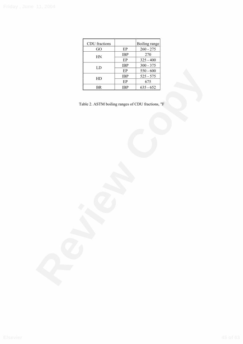
Revie
w C
opy
CDU fractions Boiling rangeGO EP 260 - 275
IBP 270 HN EP 325 - 400 IBP 300 - 375 LD EP 550 - 600 IBP 525 - 575 HD EP 675
BR IBP 635 - 652
Table 2. ASTM boiling ranges of CDU fractions, °F
45 of 63
Friday , June 11, 2004
Elsevier
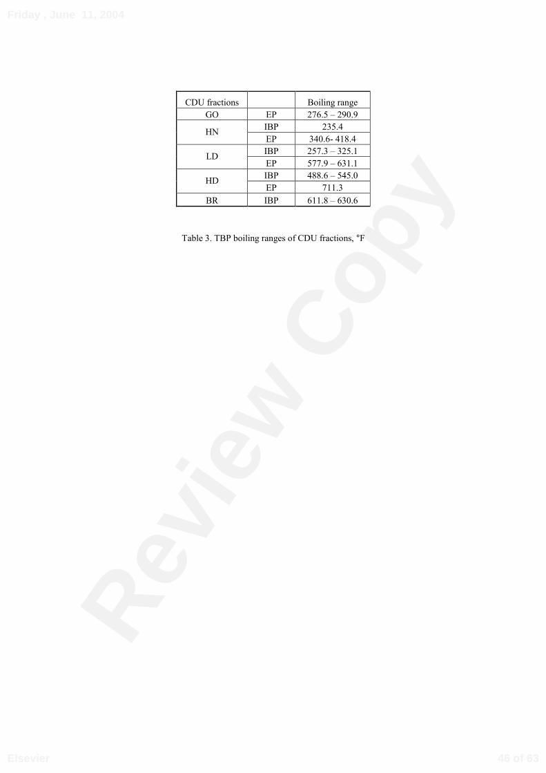
Revie
w C
opy
CDU fractions Boiling range GO EP 276.5 – 290.9
IBP 235.4 HN EP 340.6- 418.4 IBP 257.3 – 325.1 LDEP 577.9 – 631.1 IBP 488.6 – 545.0 HD EP 711.3
BR IBP 611.8 – 630.6
Table 3. TBP boiling ranges of CDU fractions, °F
46 of 63
Friday , June 11, 2004
Elsevier

Revie
w C
opy
CDU Fractions M.N., °F M.L., °F M.H., °FGO EP 276.5 290.9 290.9
IBP 235.4 235.4 235.4 HN EP 418.4 340.6 340.6 IBP 325.1 257.3 257.3 LD EP 631.1 631.1 577.9 IBP 545.0 545.0 488.6 HD EP 711.3 711.3 711.3
BR IBP 611.8 611.8 630.6
Table 4. TBP boiling ranges of CDU fractions in the three operation modes
47 of 63
Friday , June 11, 2004
Elsevier

Revie
w C
opy
GO/HN HN/LD LD/HD HD/BR
M. N. 255.9 371.8 588.0 661.6
M. L. 263.1 298.9 588.0 661.6
M. H. 263.1 298.9 533.2 670.9
Table 5. Calculated cutpoints, °F
48 of 63
Friday , June 11, 2004
Elsevier
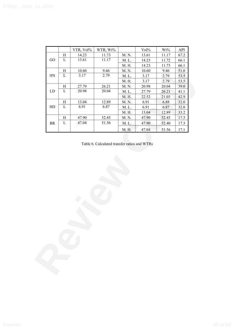
Revie
w C
opy
VTR, Vol% WTR, Wt% Vol% Wt% API H 14.23 11.73 M. N. 13.61 11.17 67.2
M. L. 14.23 11.72 66.1 GO L 13.61 11.17 M. H. 14.23 11.73 66.1
H 10.60 9.46 M. N. 10.60 9.46 51.0 M. L. 3.17 2.79 53.5 HN L 3.17 2.79 M. H. 3.17 2.79 53.5
H 27.79 26.21 M. N. 20.98 20.04 39.0 M. L. 27.79 26.21 41.1 LD L 20.98 20.04 M. H. 22.52 21.03 42.9
H 13.04 12.89 M. N. 6.91 6.88 32.0 M. L. 6.91 6.87 32.0 HD L 6.91 6.87 M. H. 13.04 12.89 33.2
H 47.90 52.45 M. N. 47.90 52.45 17.3 M. L. 47.90 52.40 17.3 BR L 47.04 51.56
M. H. 47.04 51.56 17.1
Table 6. Calculated transfer ratios and WTRs
49 of 63
Friday , June 11, 2004
Elsevier
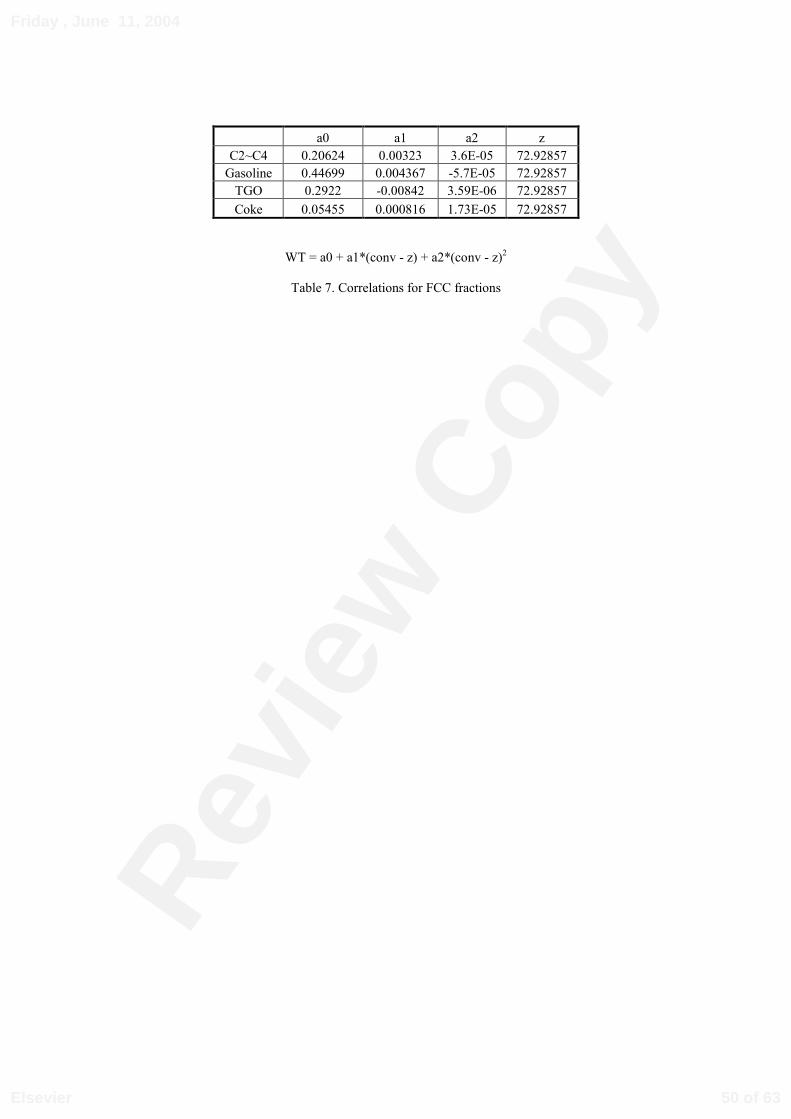
Revie
w C
opy
a0 a1 a2 z C2~C4 0.20624 0.00323 3.6E-05 72.92857
Gasoline 0.44699 0.004367 -5.7E-05 72.92857 TGO 0.2922 -0.00842 3.59E-06 72.92857 Coke 0.05455 0.000816 1.73E-05 72.92857
WT = a0 + a1*(conv - z) + a2*(conv - z)2
Table 7. Correlations for FCC fractions
50 of 63
Friday , June 11, 2004
Elsevier
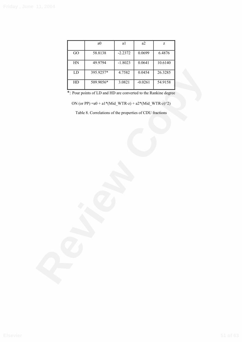
Revie
w C
opy
a0 a1 a2 z
GO 58.8138 -2.2372 0.0699 6.4876
HN 49.9794 -1.8023 0.0641 10.6140
LD 395.9257* 4.7582 0.0454 26.3285
HD 509.9056* 3.0821 -0.0261 54.9158
*: Pour points of LD and HD are converted to the Rankine degree
ON (or PP) =a0 + a1*(Mid_WTR-z) + a2*(Mid_WTR-z)^2)
Table 8. Correlations of the properties of CDU fractions
51 of 63
Friday , June 11, 2004
Elsevier

Revie
w C
opy
GO HN LD HD BR M. N. 11.17 9.46 20.04 6.88 52.45 M. L. 11.72 2.79 26.21 6.87 52.40 M. H. 11.73 2.79 21.03 12.89 51.56
Table 9. Fixed CDU fractions weight transfer ratios in the three modes, %
52 of 63
Friday , June 11, 2004
Elsevier
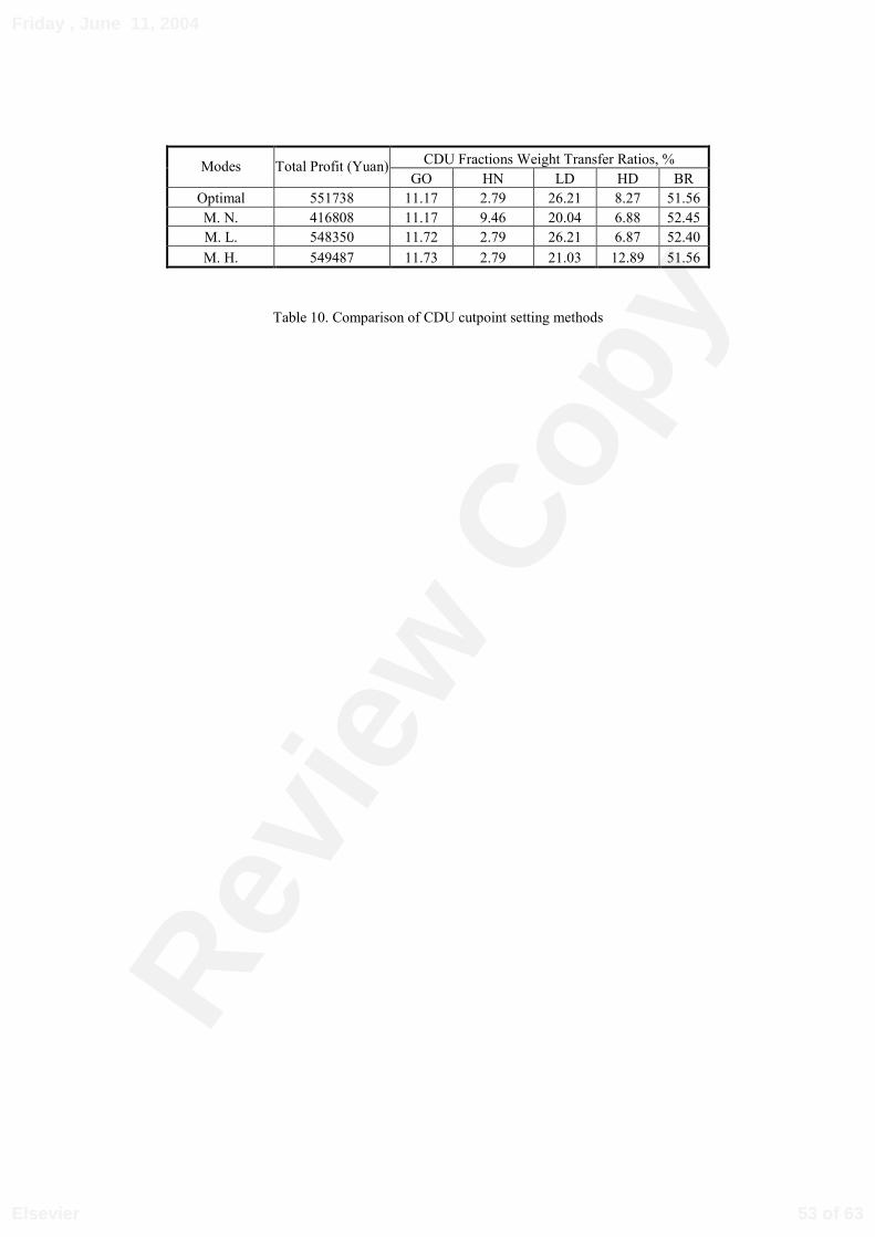
Revie
w C
opy
CDU Fractions Weight Transfer Ratios, % Modes Total Profit (Yuan)GO HN LD HD BR
Optimal 551738 11.17 2.79 26.21 8.27 51.56 M. N. 416808 11.17 9.46 20.04 6.88 52.45 M. L. 548350 11.72 2.79 26.21 6.87 52.40 M. H. 549487 11.73 2.79 21.03 12.89 51.56
Table 10. Comparison of CDU cutpoint setting methods
53 of 63
Friday , June 11, 2004
Elsevier
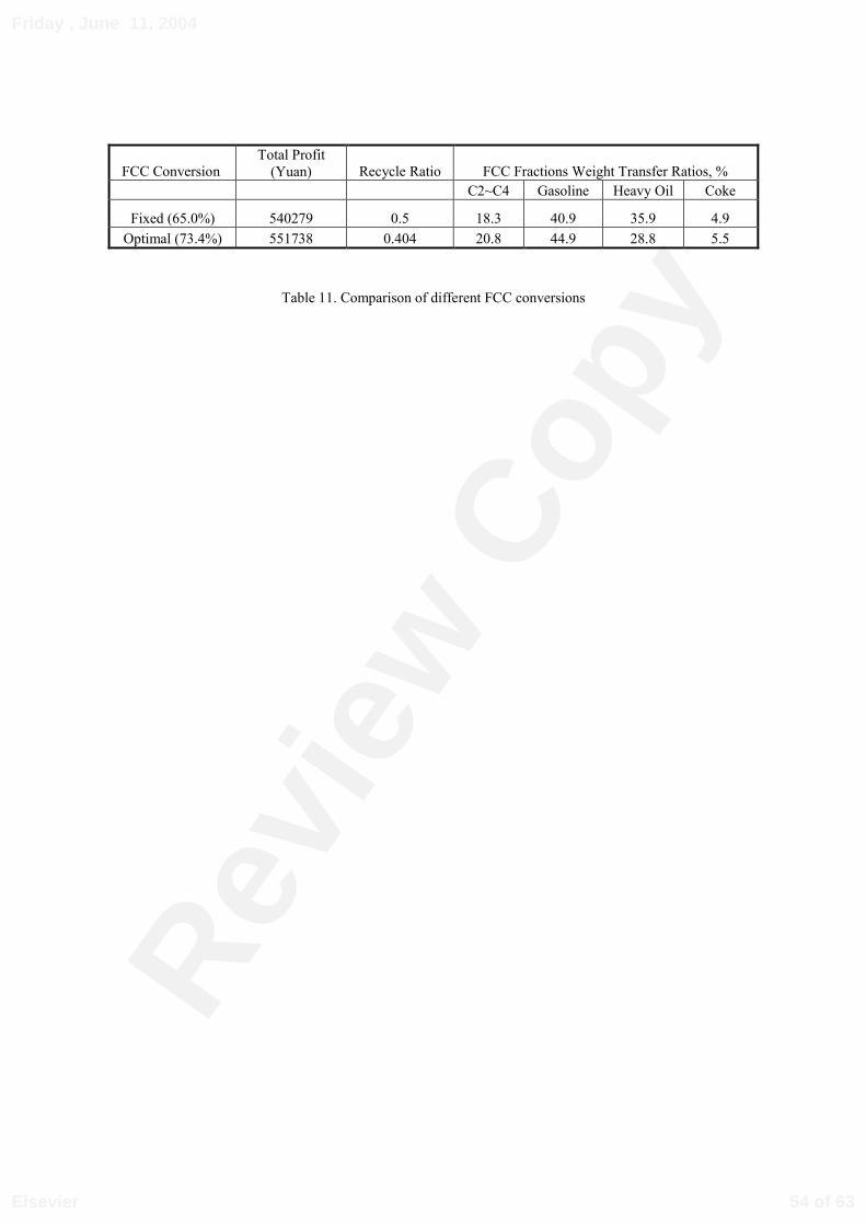
Revie
w C
opy
FCC Conversion Total Profit
(Yuan) Recycle Ratio FCC Fractions Weight Transfer Ratios, % C2~C4 Gasoline Heavy Oil Coke
Fixed (65.0%) 540279 0.5 18.3 40.9 35.9 4.9 Optimal (73.4%) 551738 0.404 20.8 44.9 28.8 5.5
Table 11. Comparison of different FCC conversions
54 of 63
Friday , June 11, 2004
Elsevier

Review Copy
Table 12. CDU fractions properties calculation
Octane Numbers (ON) or Pour Points (PP) Weight Transfer Ratios (%)Total Profit
(Yuan)GO
(ON)
HN
(ON)
LD
(PP)
HD
(PP)
GO HN LD HD BR
ON & PP Changeable 551738 60.9 46.7 -51.2 -9.7 11.17 2.79 26.21 8.27 51.56
ON & PP Estimated and Fixed 544421 50.0 65.0 -40.0 5.0 11.17 2.79 26.21 8.27 51.56
ON & PP Estimated and Fixed 581482 82.0 65.0 -40.0 5.0 11.73 2.79 26.21 7.71 51.56
55 of 63
Friday , June 11, 2004
Elsevier
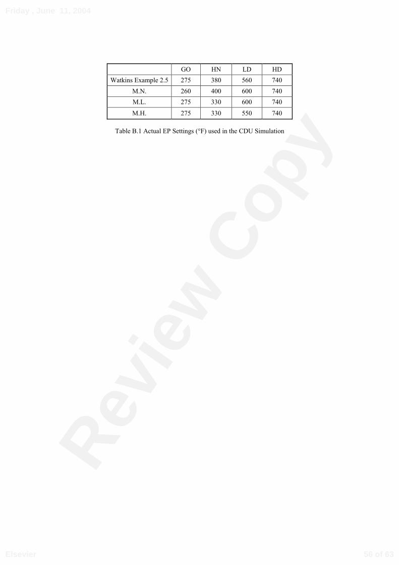
Revie
w C
opy
GO HN LD HD Watkins Example 2.5 275 380 560 740
M.N. 260 400 600 740 M.L. 275 330 600 740
M.H. 275 330 550 740
Table B.1 Actual EP Settings (°F) used in the CDU Simulation
56 of 63
Friday , June 11, 2004
Elsevier

Revie
w C
opy
Methods GO HN LD HD BR
ASPEN 142,386 113,245 203,083 123,952 682,363 Mass Flow(Ib/hr) Watkins 138,802 116,175 208,728 124,958 675,879
ASPEN 11.26 8.95 16.05 9.80 53.94
Watkins 10.98 9.19 16.51 9.88 53.45 Mass Ratio(%)
Difference,% 2.48 2.63 2.82 0.85 0.91
Table B.2 Results of CDU mass balance
57 of 63
Friday , June 11, 2004
Elsevier

Revie
w C
opy
Methods GO HN LD HD BR
ASPEN 9.87 12.66 16.97 5.30 55.20 M.N.
This Paper 11.17 9.46 20.04 6.88 52.45 ASPEN 12.04 2.45 25.47 4.58 55.46
M.L. This Paper 11.72 2.79 26.21 6.87 52.40
ASPEN 12.05 2.47 21.43 10.22 53.83 M.H.
This Paper 11.73 2.79 21.03 12.89 51.56
Table B.3 Weight Transfer Ratios of CDU Fractions by Aspen Plus simulation
58 of 63
Friday , June 11, 2004
Elsevier

Revie
w C
opy
This Paper ASPEN
H 11.73 12.05 GO L 11.17 9.87
H 9.46 12.66 HN
L 2.79 2.45
H 26.21 25.47 LD
L 20.04 16.97
H 12.89 10.22 HD
L 6.87 4.58
H 52.45 55.46 BR
L 51.56 53.83
Table B.4 WTRs of CDU Fractions
59 of 63
Friday , June 11, 2004
Elsevier
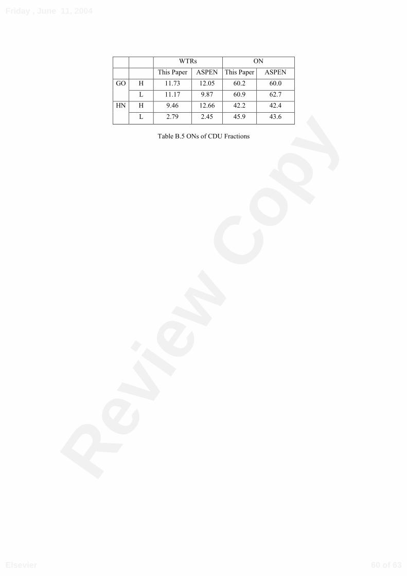
Revie
w C
opy
WTRs ON This Paper ASPEN This Paper ASPEN
H 11.73 12.05 60.2 60.0 GOL 11.17 9.87 60.9 62.7 H 9.46 12.66 42.2 42.4 HNL 2.79 2.45 45.9 43.6
Table B.5 ONs of CDU Fractions
60 of 63
Friday , June 11, 2004
Elsevier
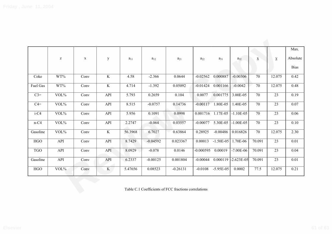
Review Copyz x y a11 a12 a21 a22 a31 a32 x y
Max.
Absolute
Bias
Coke WT% Conv K 4.58 -2.366 0.0644 -0.02562 0.000887 -0.00306 70 12.075 0.42
Fuel Gas WT% Conv K 4.714 -1.392 0.05092 -0.01424 0.001166 -0.0042 70 12.075 0.48
C3= VOL% Conv API 5.793 0.2659 0.104 0.0077 0.001775 3.00E-05 70 23 0.19
C4= VOL% Conv API 8.515 -0.0757 0.14736 -0.00117 1.80E-05 1.40E-05 70 23 0.07
i-C4 VOL% Conv API 5.956 0.1091 0.0998 0.001716 1.17E-05 -1.10E-05 70 23 0.06
n-C4 VOL% Conv API 2.2747 -0.064 0.03557 -0.00077 5.30E-05 -1.00E-05 70 23 0.10
Gasoline VOL% Conv K 56.3968 6.7027 0.63864 0.28925 -0.00486 0.016826 70 12.075 2.30
HGO API Conv API 8.7429 -0.04592 0.023367 0.00013 -1.50E-05 1.70E-06 70.091 23 0.01
TGO API Conv API 8.0929 -0.078 0.0146 -0.000595 0.00019 -7.00E-06 70.091 23 0.04
Gasoline API Conv API 6.2337 -0.00125 0.001804 -0.00044 0.000119 -2.623E-05 70.091 23 0.01
HGO VOL% Conv K 5.47656 0.08523 -0.26131 -0.0108 -5.95E-05 0.0002 77.5 12.075 0.21
Table C.1 Coefficients of FCC fractions correlations
61 of 63
Friday , June 11, 2004
Elsevier
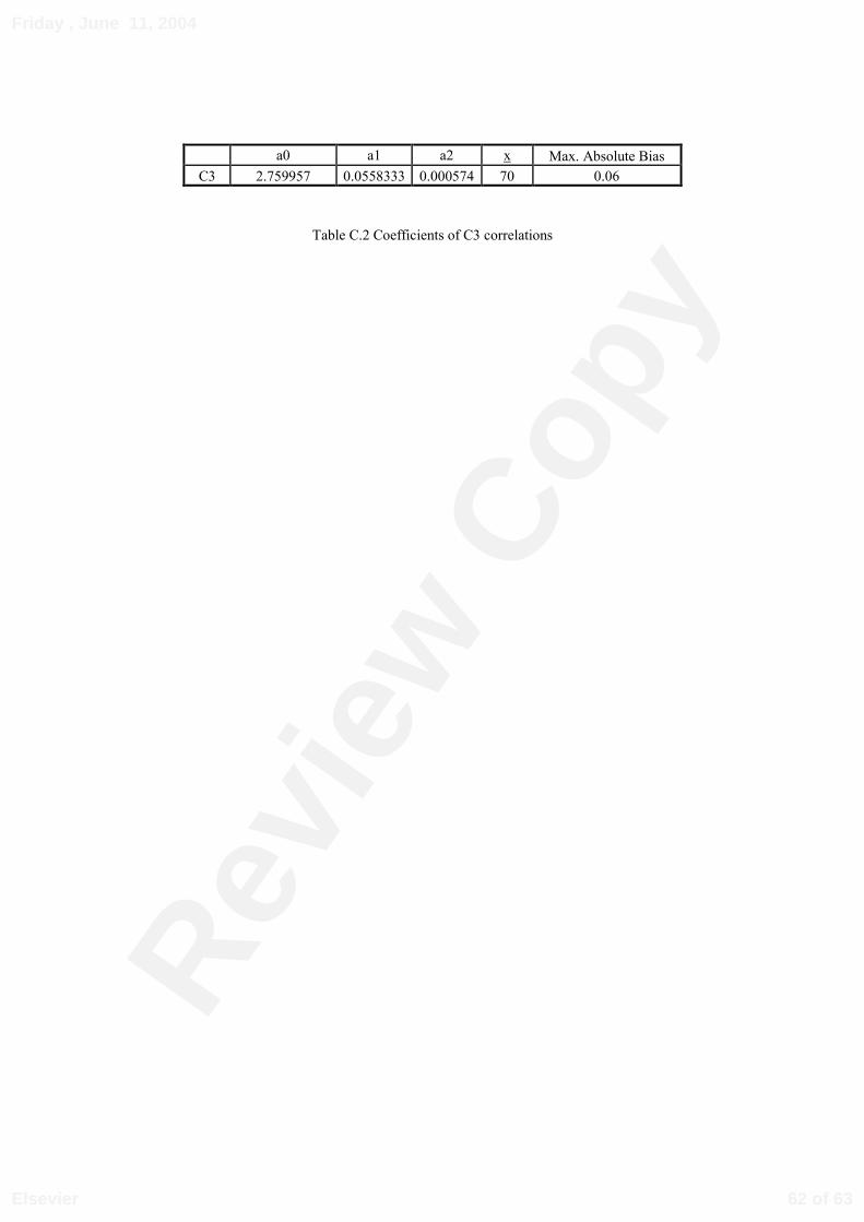
Revie
w C
opy
a0 a1 a2 x Max. Absolute Bias C3 2.759957 0.0558333 0.000574 70 0.06
Table C.2 Coefficients of C3 correlations
62 of 63
Friday , June 11, 2004
Elsevier

Revie
w C
opy
Fractions n0ns,a_dens = n1ns,a_dens = n2ns,a_dens = n3ns,a_dens =
s3 (LD) 0.8078 0.0033 -1.824E-5 26.3285 s4 (HD) 0.8818 0.0022 -1.407E-5 54.9158
Table D.1 Coefficients for specific gravities of LD and HD
63 of 63
Friday , June 11, 2004
Elsevier


