Pharmacokinetic Model for Alcohol
Nurefsan Davulcu
1324037
Fall 2014, Physics 2G03
December 8, 2014
Introduction
Pharmacokinetics
Pharmacokinetics is the study of drug absorption, distribution, metabolism, and excretion [2]. Some
common pharmacokinetic parameters are summarized in Table 1. The steady state in pharmacokinetics
occurs when the overall intake of the drug is fairly in dynamic equilibrium with its elimination [3].
Table 1: Common Parameters in Pharmacokinetic Models [3]
Characteristic Description Symbol Formula
Dose Amount of drug Administered
D
Cmax Peak plasma concentration of a drug after administration
Cmax
𝐶𝑠𝑠 Steady State Concentration
𝐶𝑠𝑠
tmax Time to reach Cmax tmax
Area under the Curve Area under the concentration-time curve
AUC
∫ 𝐶𝑑𝑡
∞
−∞
Clearance Volume of plasma cleared of the drug per unit time
CL 𝐷
𝐴𝑈𝐶
Infusion Rate The rate that a drug is administered to reach a steady state
𝑘𝑖𝑛
𝐶𝑠𝑠𝐶𝐿 =𝐶𝑠𝑠𝐷
𝐴𝑈𝐶
The parameters summarized in this table are drug related. In addition, factors depending on the
individual and their physiology have a large effect on how they metabolize a specific drug. Renal
function, genetic makeup, sex, age, obesity, hepatic failure, and dehydration are some contributing
factors [1].
A fundamental concept in pharmacokinetics is elimination of drugs from the body. In clinical practice,
this is not measured directly but is calculated by either of the following:
𝑐𝑙𝑒𝑎𝑟𝑎𝑛𝑐𝑒 = 𝐶𝐿 =𝐷
𝐴𝑈𝐶=
𝐷
∫ 𝐶𝑑𝑡∞
0
(1.1.1)
Equivalently 𝐷
𝐴𝑈𝐶=
𝐶𝑠𝑠𝐷
𝐴𝑈𝐶
𝐶𝑠𝑠=
𝑖𝑛𝑓𝑢𝑠𝑖𝑜𝑛 𝑟𝑎𝑡𝑒
𝐶𝑠𝑠 (1.1.2)
From these equations, it can be concluded that the elimination rate decreases as the AUC increases.
Equivalently, for a higher concentration of the drug for a given dose, the elimination will be slower [2].
Pharmacokinetic Models
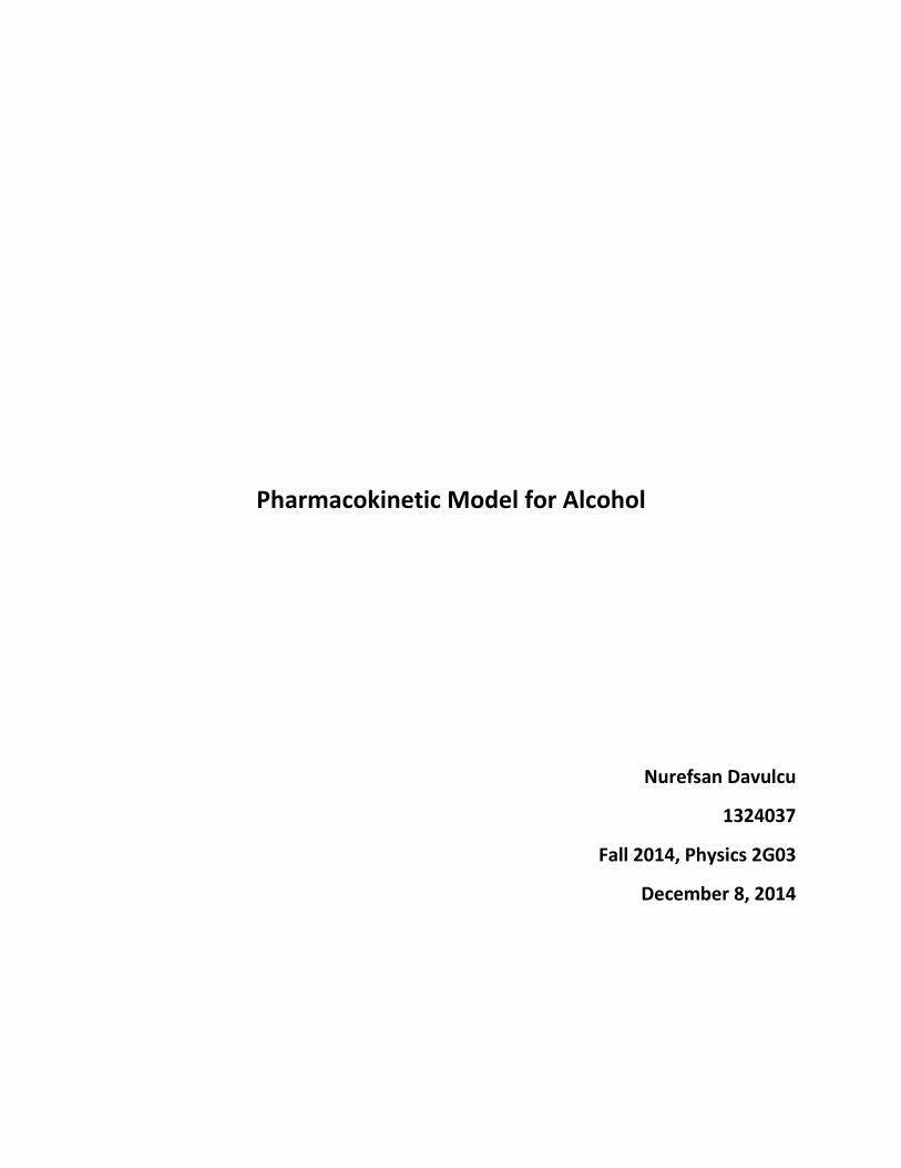
Many pharmacokinetic models follow the laws of first
order kinetics (linear pharmacokinetic models) , that is: 𝑑𝐶
𝑑𝑡= −𝑘𝐶 (1.2.1)
which has an explicit solution: 𝐶(𝑡) = 𝐶𝑜𝑒−𝑘𝑡
𝐶𝑜 in this case is 𝐷
𝑉 so 𝐶(𝑡) =
𝐷
𝑉𝑒−𝑘𝑡 (1.2.2)
This is shown graphically in Figure 1.
However, this model makes the assumption that the drug
is consumed and distributed instantaneously. These
assumptions are often not valid. A better model involves
accounting for the consumption period.
Consumption Period: 𝐶(𝑡) =𝐷
𝑉𝐾𝑇(1 − 𝑒−𝑘𝑡) where T=consumption period (2.3)
Post-consumption/ Elimination Period: 𝑑𝐶
𝑑𝑡= 𝐶(𝑇)𝑒−𝑘(𝑡−𝑇) (2.4)
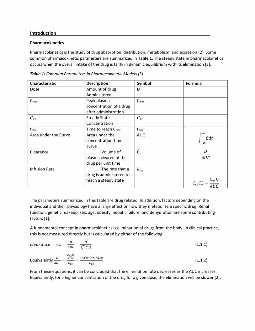
The elimination period is best fit to a multicompartment model (represented by more than one
equation) such as the one shown in Figure 2 [2].
Figure 2: Elimination Period for Multicompartment Pharmocokinetic Model [2]
Pharmacokinetic Models of Alcohol
A mathematical model for alcohol metabolism could be useful in forensics and legal medicine, for
example, in the investigation of alcohol-related crimes such as drunk driving or drug-related sexual
assaults. In the case of drunk driving, a blood sample may not be taken until several hours after the
offence was committed, but the suspect's blood alcohol concentration at the time of driving is needed
which requires a back-calculation. An accurate mathematical model to predict the BAC (Blood Alcohol
Concentration) would be needed to perform the back-calculation [4].
Figure 1: First-order Pharmocokinetic Model. C0 represents the initial concentration, assuming instantaneous administration and distribution [2].

I will compare my model to several sets of experimental data and computer models that were under
different testing conditions to see which testing conditions are most accurately represented by the
model and to identify limitations of the model.
To describe my model and the studies it will be compared to, it is important to understand the
parameters. These are summarized in Table 2.
Table 2: Definition of Common Parameters used in Pharmacokinetics of Alcohol [4]
Parameter Symbol Description Units
Disappearance Rate of Alcohol from the Blood
𝛽-slope Amount of Alcohol by Mass Eliminated for a given Volume of Blood per time step
mg/100ml/hour
Volume of Distribution (Also called Widmark's Rho Factor)
Vd Ratio between the concentration of alcohol in the body and the concentration in the blood. Alcohol mixes with total body water without binding to plasma proteins therefore this ratio is equivalent to the ratio of water content of the blood to the water content of the rest of the body.
g/kg, L/kg mg/100ml
Blood Alcohol Concentration BAC Amount of Alcohol by Mass present in a Volume of Whole Blood
g/L
A typical concentration-time profile is shown in Figure 3.
Figure 3: Pharmocokinetic Model for Alcohol for a male subject who drank neat whisky (0.80g ethanol/kg body weight) on an empty stomach. There is a rising BAC during absorption to reach a peack concentration (Cmax) at time tmax followed by the elimination phase. The elimination phase follows zero-order kinetics i.e. linear. as shown by Pearson's r=0.98. Linear regression analysis given the y-intercept (Co) and x-intercept (Mino) allowing determination of the elimination rate from blood (𝜷-slope) and distribution volume as shown (These are defined in Table 2) [4].

Hundreds of studies have been made of the pharmacokinetics of alcohol under various testing
conditions and the such as varying alcohol dose, speed of drinking, type of alcoholic beverage, and the
fed or fasted states of the subjects [4]. The sample of subjects chosen also varies between studies for
sample size, subject gender, age, drinking history, and physiology.
Widmark and Other Similiar Models
The first pharmacokinetic study on alcohol was done by Erik MP Widmark in the 1920s. Widmark
surveyed 20 men and 10 women who were all moderate drinkers in the following strictly controlled
drinking conditions:
Rapid drinking (5-15 minutes)
Consumption of alcohol on an empty stomach usually after an overnight (10h fast) and not 2-3h
after eating
Administration of a moderate dose (0.5-1.0 g/kg) as spirits and not as beer or wine
Blood-ethanol was determined in capillary (fingertip) blood
After Widmark, studies by Osterlind et al., Jokipii, and Jones were also done following the same drinking
conditions to try to duplicate his results. A summary of the results from Widmark and the following
three studies performed in the same drinking conditions are summarized in Table 3 [4].
Table 3: Average Elimination Rates of alcohol from blood (𝛽) and volume of distribution (Vd, rho factor)
from Four Studies (Widmark, Osterlind et al., Jokipii, and Jones) for Healthy Men and Women after they
drank a moderate dose of alcohol after an overnight fast. Values are mean ∓standard deviation [4].
Total Males Assessed
Average Male 𝛽-slope
Average Male Vd (distribution volume, rho factor)
Total Females Assessed
Average Female 𝛽-slope
Average Female Vd
(distribution volume, rho factor)
97 13.3 ∓ 2.9 0.68 ∓ 0.063 53 15.1 ∓ 2.02 0.59 ∓ 0.078 Widmark used his results to develop an algebraic equation to estimate any one of 6 variables given the
other 5 [6].
𝐴 =𝑊𝑟(𝐶𝑡+𝛽𝑡)
0.8𝑧 (1.3.1)
A=the number of drinks consumed
W=body weight in ounces
r=constant relating the distribution of water in the body in L/kg
Ct=the blood alcohol concentration (BAC) in Kg/L
𝛽=the alcohol elimination rate in Kg/L
t=time since the first drink in hours
z=the fluid ounces of alcohol per drink

My Model [5]
Constants
b =body water per given weight, for male: 0.7 L/kg=0.317544 L/pound, for female: 0.6 L/kg=0.2721552
L/pound (Jones, 2010)
v =gender parameter (male=4, female=0.4)
Variables (Also refer to Table 2 and Figure 3)
C =concentration of alcohol in the blood (BAC, % g/dL)
d =amount of alcohol consumed (unitless, ex: 5 drinks)
s =the length of the alcohol consumption period (hours)
w =weight (pounds)
𝑢 =𝑑
𝑏 × 𝑤 × 𝑠
𝛼=liver function parameter (higher value indicates better liver function)
𝛽=kidney function parameter (higher value indicates better kidney function)
t =time (hours)
Equations
During the Consumption Period: 𝑑𝐶
𝑑𝑡= 𝑢 −
𝛼×𝐶
𝑎+𝛽 , 0 ≤ 𝑡 ≤ 𝑠, 𝑎(0) = 0 (2.1.1)
This model is used to find the peak alcohol concentration (𝐶𝑚𝑎𝑥) which is assumed in this model to
occur at the end of the alcohol consumption period, i.e. 𝐶𝑚𝑎𝑥 = 𝐶(𝑠). This is a good approximation for
large s, however, 𝐶𝑚𝑎𝑥 actually occurs slightly after the end of alcohol consumption i.e. 𝑡𝑚𝑎𝑥 > 𝑠
During the Elimination Period: 𝑑𝐶
𝑑𝑡= −
𝛼×𝐶
𝑎+𝛽 , 𝑠 < 𝑡, 𝑎(𝑠) = 𝐶𝑚𝑎𝑥 (2.1.2)
The Program Code (cd project, make plot, plot)
AlcoholMetabolism.c My program uses a 4-step Runge-Kutta technique to integrate equations 2.1.1 and
2.1.2 (this is implemented in function a). Equations 2.1.1 and 2.1.2 are functions consumption and
elimination, respectively. The function a calls functions consumption and elimination at every step in the
Runge Kutta. The final time and BAC values are stored in arrays t and at. The arrays are written to data
files according to gender (ex: if we call function a twice for 2 females, it will store these in data files
female_output1.data and female_output2.data). This is specified by the float x and float y parameters in
function a. Float x indicates whether we want data for female and male(x=2), only male(x=1), or only
female(x=1). Float y indicates whether it is the first set of data or second set of data so that the function
knows to not overwrite the data already stored in the gender specific file. All functions in
AlcoholMetabolism.c are included in the header file AlcoholMetabolism.h.
plot.c There are four functions to vary a specific parameter while keeping the other parameters
constant (testgender,testdrink,testweight,testliver). I chose to vary these parameters so that I could
compare to the results from [5]. Each of the functions call the plot function for plotting. In the main
function, one of the calls to test (parameter name) is left uncommented to test for that parameter.
Results
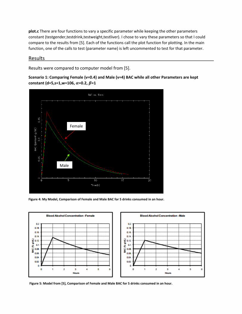
Results were compared to computer model from [5].
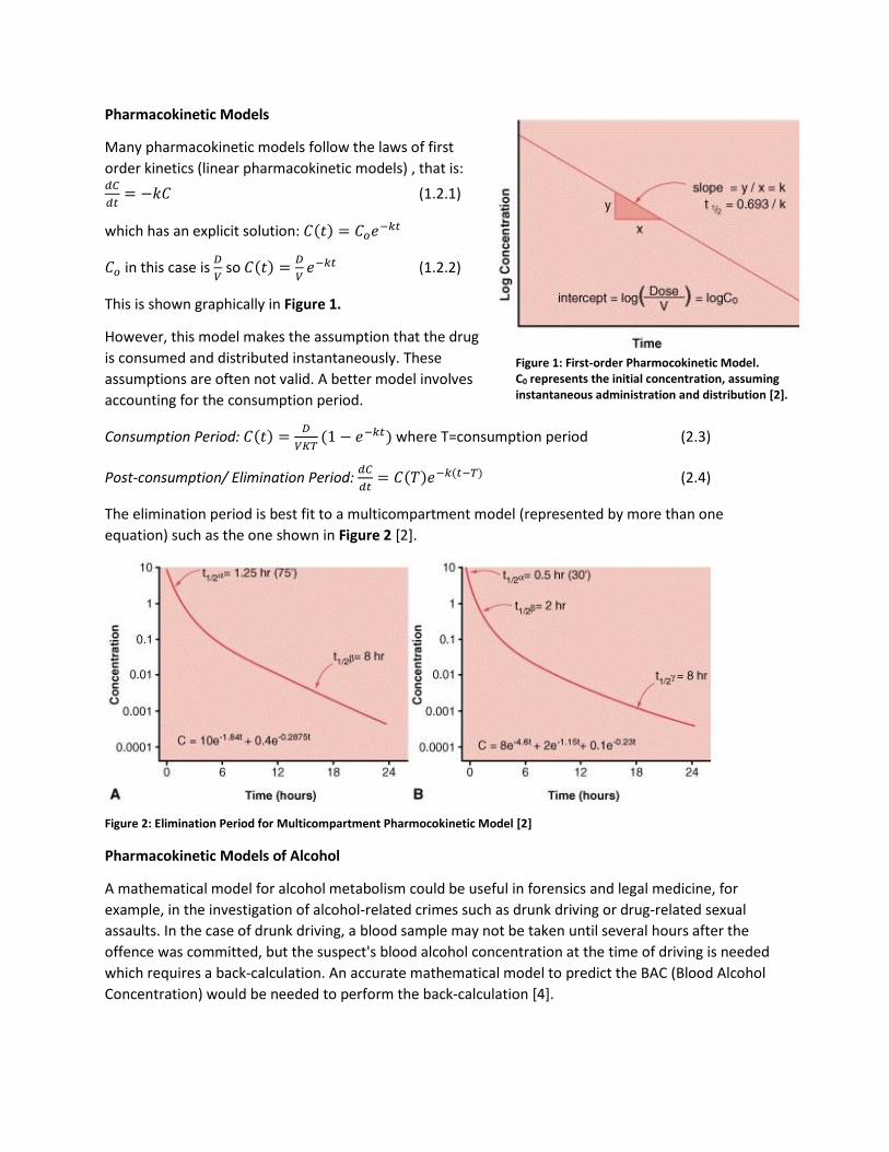
Scenario 1: Comparing Female (v=0.4) and Male (v=4) BAC while all other Parameters are kept
constant (d=5,s=1,w=106, 𝜶=0.2, 𝜷=1
Figure 4: My Model, Comparison of Female and Male BAC for 5 drinks consumed in an hour.
Female
Male
Figure 5: Model from [5], Comparison of Female and Male BAC for 5 drinks consumed in an hour.

Scenario 2: Comparing BAC of Two Males (v=4) with Different Weights (w=150 and w=250) while all
other Parameters are kept constant (d=4,s=3, 𝜶=0.2, 𝜷=1)
Figure 6: My model, Comparing BAC of two Males with Different Weights for Four Drinks consumed in 3 hours.
Figure 7: Model from [5], Comparing BAC of two Males with Different Weights for Four Drinks consumed in 3 hours.
150 pounds
250 pounds

Scenario 3: Comparing BAC of two females consuming different Amounts of Alcohol (d=2 and d=5)
while all other Parameters are kept constant (s=4,w=140, 𝜶=0.2, 𝜷=1)
Figure 9: My Model, Comparing BAC of Two Females, one consumed 2 drinks and the other consumed 5 over 4 hours.
Figure 10: Model from [5], Comparing BAC of Two Females, one consumed 2 drinks and the other consumed 5 over 4 hours.
5 drinks
2 drinks
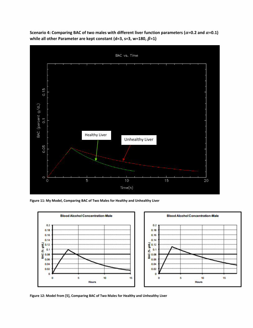
Scenario 4: Comparing BAC of two males with different liver function parameters (𝜶=0.2 and 𝜶=0.1)
while all other Parameter are kept constant (d=3, s=3, w=180, 𝜷=1)
Figure 11: My Model, Comparing BAC of Two Males for Healthy and Unhealthy Liver
Figure 12: Model from [5], Comparing BAC of Two Males for Healthy and Unhealthy Liver
Healthy Liver Unhealthy Liver
Analysis of Results
My model was consistent with the model from [5]. They both demonstrated that females have a higher
peak concentration (Cmax) and a slower rate of alcohol metabolism (longer time to reach Mino) compared
to men. Therefore 𝛽-slope (elimination rate) for females is greater than the 𝛽-slope for males. This
result is also consistent with the experimental data presented in Table 3.
In addition, the Cmax and β-slope were less for a subject that weighed more compared to a subject that
weighed less. It also took a longer time to reach Mino (slower rate of alcohol metabolism).
Furthermore, a higher dosage of alcohol resulted in a higher Cmax, β-slope and a longer time to reach
Mino.
Lastly, a healthy liver and unhealthy liver had Cmax that were almost the same for my model and very
close for the model from [5]. However, the healthy river was better at eliminating the alcohol as was
expected (lower 𝛽-slope and less time to reach Mino).
As stated in the introduction, the elimination period should follow zero-order kinetics (linear) however,
my model’s elimination period would fit a curve better than a linear model.
Extensions to my Model
In terms of the program code, a line of best fit could be plotted on to the BAC-time curves such as in
Figure 3 and extrapolation
could be used to determine the
exact values of Mino, Co, and β-
slope. Pearson’s R could be
calculated to determine how
closely the elimination period
was to linear which would
further test the accuracy of the
model. In addition, the BAC
values at each time step could
be plugged into equation 2.1.2
(elimination period) to
determine the elimination rates
precisely at each time step (per
hour).
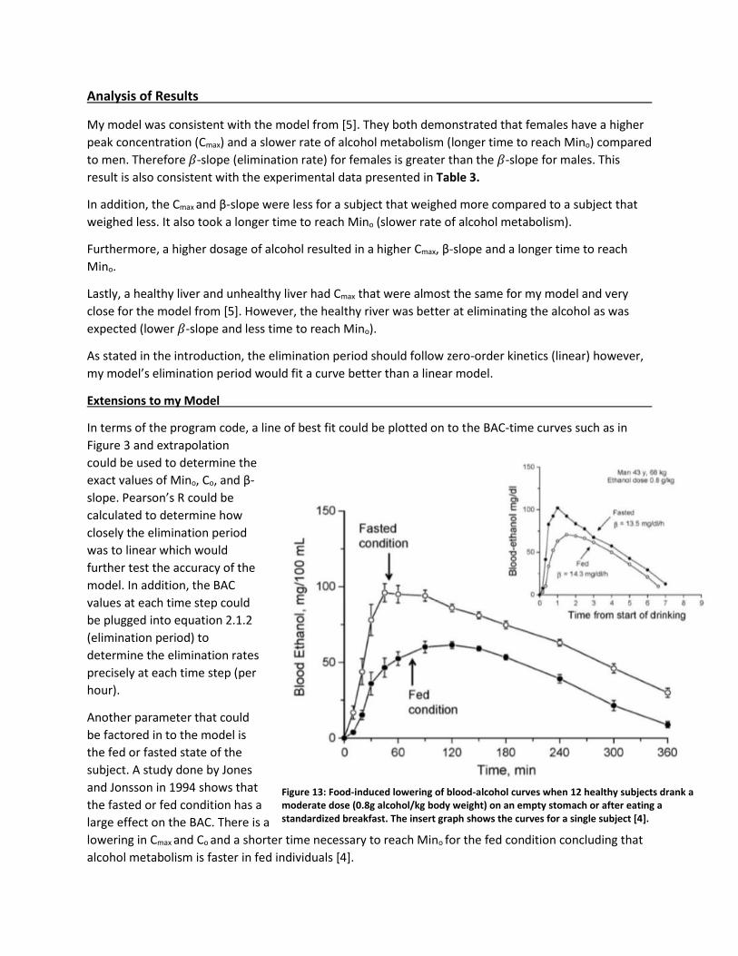
Another parameter that could
be factored in to the model is
the fed or fasted state of the
subject. A study done by Jones
and Jonsson in 1994 shows that
the fasted or fed condition has a
large effect on the BAC. There is a
lowering in Cmax and Co and a shorter time necessary to reach Mino for the fed condition concluding that
alcohol metabolism is faster in fed individuals [4].
Figure 13: Food-induced lowering of blood-alcohol curves when 12 healthy subjects drank a moderate dose (0.8g alcohol/kg body weight) on an empty stomach or after eating a standardized breakfast. The insert graph shows the curves for a single subject [4].

References
[1] Le J., (2014, May). Pharmacokinetics. The Merck Manual. Whitehouse Station, New Jersey. [Online]
Available
http://www.merckmanuals.com/professional/clinical_pharmacology/pharmacokinetics/overview_of_ph
armacokinetics.html
[2] Ratain, M.J., William K.P., (2003). Cancer Medicine. (6). [Online]. Available:
http://www.ncbi.nlm.nih.gov/books/NBK12815/
[3] Wikipedia contributors. (2014, December). Pharmacokinetics. Wikipedia. [Online] Available:
http://en.wikipedia.org/wiki/Pharmacokinetics
[4] Jones A.W. (2010, March). “Evidence-based survey of the elimination rates of ethanol from blood
applications in forensic casework.” Forensic Science International. [Online] 200(1-3), pp. 1-20. doi:
10.1016/j.forsciint.2010.02.021
[5] Elgindi M.B.M., Kouba S.J., Langer R.W. Exploring Mathematical Models for Calculating Blood Alcohol
Concentration. University of Wisconsin. Eau-Claire, WI. [Online]
[6] Widmark, E.M.P., “Principles and Applications of Medicolegal Alcohol Determination,” Journal of
Applied Toxicology, vol. 2, no. 5, pp. 4, Oct. 1982.


