Chapter1 Chapter2 Chapter3 Chapter4 Chapter5
Ph.D Thesis
Efficient Bayesian Estimation of Time SeriesModels and Its Applications
Yuta KUROSE
Graduate School of Economics, University of Tokyo
January 23, 2013
1 / 80
Chapter1 Chapter2 Chapter3 Chapter4 Chapter5
Outline
Chapter1 Overview
Chapter2 Bayesian analysis of time-varying quantiles using a smoothingspline
Chapter3 Dynamic equicorrelation stochastic volatility
Chapter4 Realized stochastic volatility with dynamic equicorrelation andcross leverage
Chapter5 Dynamic block-equicorrelation, realized stochastic volatilityand cross leverage
2 / 80
Chapter1 Chapter2 Chapter3 Chapter4 Chapter5
Overview
• Around 1990, the Markov chain Monte Carlo (MCMC)“revolution” occurred in Bayesian computing.
• e.g., the Gibbs sampler and the Metropolis-Hastings (MH)algorithm can greatly facilitate calculation of the integrals.
• With the development of high-power computing, researchersin diverse areas are trying to conduct a statistical modelingusing Bayesian approach.(e.g., Gelman et al (2003), Koop et al (2007))
3 / 80
Chapter1 Chapter2 Chapter3 Chapter4 Chapter5
Overview
• Time series modeling of economic and financial data · · ·the existence of so many time-dependent latent variables, e.g.,the mean, the variance and the covariance or the quantile.
• Need to calculate the integral of the likelihood function interms of a large number of such latent variables(maximizing the likelihood — very difficult)
• −→ Since MCMC methods enables evaluation of the integral,we take the Bayesian approach in this thesis.
4 / 80
Chapter1 Chapter2 Chapter3 Chapter4 Chapter5
Overview
• Unobserved parameters in time series models are oftentime-dependent and highly-correlated
• Many researchers take a Bayesian approach and propose aMCMC algorithms to draw samples from the posterior of theparameters, but part of them are known to be inefficient.
• This thesis provides Bayesian analyses of four time seriesmodels and also develops the fast and efficient estimationalgorithm using MCMC method.
• Our models with time-dependent latent variables are given inthe state space form (Durbin and Koopman (2001)).
• Furthermore, empirical studies are presented using economicand financial time series datasets.
5 / 80
Chapter1 Chapter2 Chapter3 Chapter4 Chapter5
Chapter2
Bayesian analysis of time-varying quantiles using asmoothing spline
6 / 80

Chapter1 Chapter2 Chapter3 Chapter4 Chapter5
Introduction
• Tail quantiles are especially important for financial riskmanagement or policy evaluation
• e.g., the Value at Risk (VaR) — one of the well-known riskmeasures that are associated with an asset or a portfolio ofassets
• time-varying quantiles of the dependent variables: ConditionalAutoregressive Value at Risk (CAViaR) model (Engle andManganelli (2004)), Quantile Autoregressive (QAR) model(Koenker and Xiao (2006)) and Dynamic Additive Quantile(DAQ) model (Gourieroux and Jasiak (2008)),threshold-CAViaR model (Gerlach et al (2011))
7 / 80
Chapter1 Chapter2 Chapter3 Chapter4 Chapter5
Quantile regression model
• yt : dependent variable at time t with distribution functionF (y) = Pr(yt ≤ y)
• Define a τ -quantile as
ξ(τ) := F−1(τ) = infy |F (y) ≥ τ, (1)
• For any fixed 0 < τ < 1, and we define the loss function,called a “check function” as
ρτ (u) = (τ − I(u < 0))(u). (2)
• The expected loss,
E(ρτ (yt − ξ(τ))), (3)
is minimized when ξ(τ) satisfies F (ξ(τ)) = τ .(Koenker and Bassett (1978))
8 / 80
Chapter1 Chapter2 Chapter3 Chapter4 Chapter5
Quantile regression model
• Assume that yt is i.i.d. with the probability density functiongiven ξ(τ),
f (yt |ξ(τ)) =τ(1− τ)
λexp
(− 1
λρτ (yt − ξ(τ))
), (4)
(asymmetric double exponential (or asymmetric Laplace)density)
• Note that ξ(τ) maximizes the logarithm of this densityfunction and minimizes the expected loss function, (2.3).
• Yu and Moyeed (2001) described an MCMC algorithm for thequantile regression using a Bayesian approach.
9 / 80
Chapter1 Chapter2 Chapter3 Chapter4 Chapter5
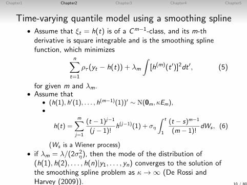
Time-varying quantile model using a smoothing spline• Assume that ξt = h(t) is of a Cm−1-class, and its m-thderivative is square integrable and is the smoothing splinefunction, which minimizes
n∑t=1
ρτ (yt − h(t)) + λm
∫[h(m)(t ′)]2dt ′, (5)
for given m and λm.• Assume that
• (h(1), h′(1), . . . , h(m−1)(1))′ ∼ N(0m, κEm),•
h(t) =m∑j=1
(t − 1)j−1
(j − 1)!h(j−1)(1) + ση
∫ t
1
(t − s)m−1
(m − 1)!dWs , (6)
(Ws is a Wiener process)
• if λm = λ/(2σ2η), then the mode of the distribution of
(h(1), h(2), . . . , h(n)|y1, . . . , yn) converges to the solution ofthe smoothing spline problem as κ → ∞ (De Rossi andHarvey (2009)). 10 / 80
Chapter1 Chapter2 Chapter3 Chapter4 Chapter5
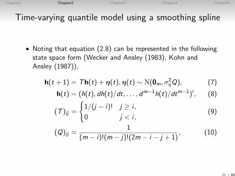
Time-varying quantile model using a smoothing spline
• Noting that equation (2.8) can be represented in the followingstate space form (Wecker and Ansley (1983), Kohn andAnsley (1987)),
h(t + 1) = Th(t) + η(t),η(t) ∼ N(0m, σ2ηQ), (7)
h(t) = (h(t), dh(t)/dt, . . . , dm−1h(t)/dtm−1)′, (8)
(T )ij =
1/(j − i)! j ≥ i ,
0 j < i ,(9)
(Q)ij =1
(m − i)!(m − j)!(2m − i − j + 1), (10)
11 / 80
Chapter1 Chapter2 Chapter3 Chapter4 Chapter5
Time-varying quantile model using a smoothing spline
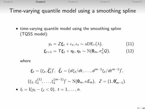
• time-varying quantile model using the smoothing spline(TQSS model):
yt = Zξt + εt , εt ∼ aDEτ (λ), (11)
ξt+1 = Tξt + ηt ,ηt ∼ N(0m, σ2ηQ), (12)
where
ξt = (ξt , ξ′t)
′, ξt = (dξt/dt, . . . , dm−1ξt/dt
m−1)′,
(ξ1, ξ(1)1 , . . . , ξ
(m−1)1 )′ ∼ N(0m, κEm), Z = (1, 0′m−1).
• It = I(yt − ξt < 0), t = 1, . . . , n.
12 / 80
Chapter1 Chapter2 Chapter3 Chapter4 Chapter5
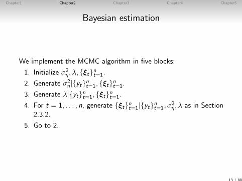
Bayesian estimation
We implement the MCMC algorithm in five blocks:
1. Initialize σ2η, λ, ξtnt=1.
2. Generate σ2η|ytnt=1, ξtnt=1.
3. Generate λ|ytnt=1, ξtnt=1.
4. For t = 1, . . . , n, generate ξtnt=1|ytnt=1, σ2η, λ as in Section
2.3.2.
5. Go to 2.
13 / 80
Chapter1 Chapter2 Chapter3 Chapter4 Chapter5
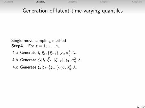
Generation of latent time-varying quantiles
Single-move sampling methodStep4. For t = 1, . . . , n,
4.a Generate It |ξt , ξ−t, yt , σ2η, λ.
4.b Generate ξt |It , ξt , ξ−t, yt , σ2η, λ.
4.c Generate ξt |ξt , ξ−t, yt , σ2η, λ.
14 / 80
Chapter1 Chapter2 Chapter3 Chapter4 Chapter5
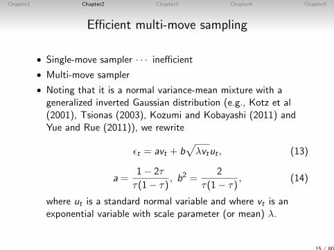
Efficient multi-move sampling
• Single-move sampler · · · inefficient
• Multi-move sampler
• Noting that it is a normal variance-mean mixture with ageneralized inverted Gaussian distribution (e.g., Kotz et al(2001), Tsionas (2003), Kozumi and Kobayashi (2011) andYue and Rue (2011)), we rewrite
εt = avt + b√
λvtut , (13)
a =1− 2τ
τ(1− τ), b2 =
2
τ(1− τ), (14)
where ut is a standard normal variable and where vt is anexponential variable with scale parameter (or mean) λ.
15 / 80
Chapter1 Chapter2 Chapter3 Chapter4 Chapter5
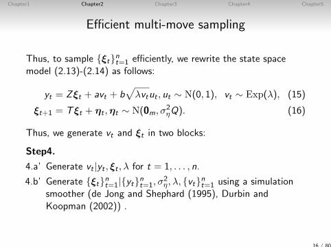
Efficient multi-move sampling
Thus, to sample ξtnt=1 efficiently, we rewrite the state spacemodel (2.13)-(2.14) as follows:
yt = Zξt + avt + b√
λvtut , ut ∼ N(0, 1), vt ∼ Exp(λ), (15)
ξt+1 = Tξt + ηt ,ηt ∼ N(0m, σ2ηQ). (16)
Thus, we generate vt and ξt in two blocks:
Step4.
4.a’ Generate vt |yt , ξt , λ for t = 1, . . . , n.
4.b’ Generate ξtnt=1|ytnt=1, σ2η, λ, vtnt=1 using a simulation
smoother (de Jong and Shephard (1995), Durbin andKoopman (2002)) .
16 / 80
Chapter1 Chapter2 Chapter3 Chapter4 Chapter5
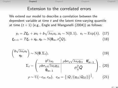
Extension to the correlated errors
We extend our model to describe a correlation between thedependent variable at time t and the latent time-varying quantileat time (t + 1) (e.g., Engle and Manganelli (2004)) as follows:
yt = Zξt + avt + b√
λvtut , ut ∼ N(0, 1), vt ∼ Exp(λ), (17)
ξt+1 = Tξt + ηt ,ηt ∼ N(0m, σ2ηQ), (18)
(b√λvtutηt
)∼ N(0,Σt), (19)
Σt =
b2λvt ρbση√λvtq11 0′m−1
ρbση√λvtq11
0m−1σ2ηQ
, (20)
ρ ∼ U(−cm, cm), cm =|Q|/(q11|Q22|)
12 , (21)
17 / 80
Chapter1 Chapter2 Chapter3 Chapter4 Chapter5
Extension to the correlated errors
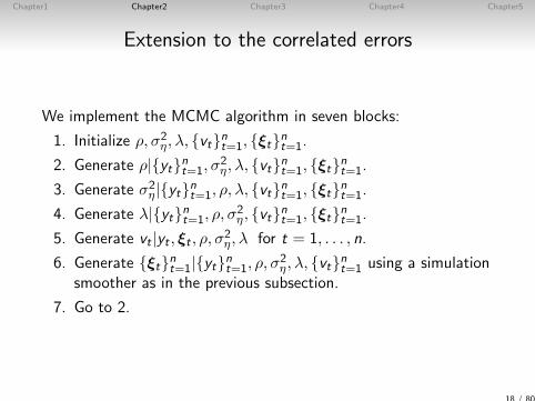
We implement the MCMC algorithm in seven blocks:
1. Initialize ρ, σ2η, λ, vtnt=1, ξtnt=1.
2. Generate ρ|ytnt=1, σ2η, λ, vtnt=1, ξtnt=1.
3. Generate σ2η|ytnt=1, ρ, λ, vtnt=1, ξtnt=1.
4. Generate λ|ytnt=1, ρ, σ2η, vtnt=1, ξtnt=1.
5. Generate vt |yt , ξt , ρ, σ2η, λ for t = 1, . . . , n.
6. Generate ξtnt=1|ytnt=1, ρ, σ2η, λ, vtnt=1 using a simulation
smoother as in the previous subsection.
7. Go to 2.
18 / 80
Chapter1 Chapter2 Chapter3 Chapter4 Chapter5
Illustrative examples using simulated data
• Simulation data: n = 300 for each τ .
• Using the single-move sampler, we generate 600,000(450,000) MCMC samples after discarding the first 1,000(1,000) samples as the burn-in period for τ = 0.1 (τ = 0.9).
• The multi-move sampler is used to generate 30,000 (15,000)MCMC samples after discarding the first 1,000 (1,000)samples as the burn-in period for τ = 0.1 (τ = 0.9).
• The inefficiency factor is defined as 1 + 2∑∞
g=1 ρ(g) (ρ(g) isthe sample autocorrelation at lag g). This is interpreted asthe ratio of the numerical variance of the posterior mean fromthe chain to the variance of the posterior mean fromhypothetical uncorrelated draws.
19 / 80
Chapter1 Chapter2 Chapter3 Chapter4 Chapter5
Illustrative examples using simulated data
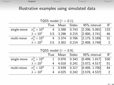
TQSS model (τ = 0.1).True Mean Stdev 95% interval IF
single-move σ2η × 103 4 3.398 0.743 [2.206, 5.091] 133
λ× 102 3.5 3.296 0.215 [2.900, 3.741] 46
multi-move σ2η × 103 4 3.374 0.766 [2.175, 5.169] 31
λ× 102 3.5 3.302 0.214 [2.908, 3.748] 2
TQSS model (τ = 0.9).True Mean Stdev 95% interval IF
single-move σ2η × 104 1 0.976 0.343 [0.499, 1.817] 530
λ× 102 4 4.018 0.241 [3.572, 4.517] 51
multi-move σ2η × 104 1 0.939 0.317 [0.495, 1.700] 44
λ× 102 4 4.025 0.242 [3.578, 4.537] 2
20 / 80
Chapter1 Chapter2 Chapter3 Chapter4 Chapter5
Empirical study
• Data — The upper and the lower tails of the distribution ofthe inflation rate of Japan, using the rate of change for thedomestic Corporate Goods Price Index (CGPI) excluding theconsumption tax for all commodities of Japan. The rate ofchange is calculated as yt = 100× (log pt − log pt−1).
• We consider the following two sample periods:
Period (I) : February, 1985 – June, 2008 (281 months) and
Period (II) : February, 1985 – January, 2010 (300 months).
• We set m = 2 and κ = 100.
• We generate 60,000 (30,000, 30,000) MCMC samples for themodel without correlations for τ = 0.1 (τ = 0.5, τ = 0.9)..
• We generate 60,000 (240,000, 240,000) MCMC samples forthe model with correlations for τ = 0.1 (τ = 0.5, τ = 0.9).
21 / 80
Chapter1 Chapter2 Chapter3 Chapter4 Chapter5
CAViaR model (Benchmark)
• As a benchmark, we consider the following asymmetric slopeCAViaR model discussed in Engle and Manganelli (2004):
ξt+1 = β1 + β2ξt + β3y+t + β4y
−t , (22)
where y+t = max(yt , 0) and y−t = −min(yt , 0) to modelasymmetry of the dynamics of the quantile.
22 / 80
Chapter1 Chapter2 Chapter3 Chapter4 Chapter5
Estimation results
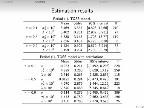
Period (I). TQSS model.Mean Stdev 95% interval IF
τ = 0.1 σ2η × 104 3.469 3.355 [0.523, 12.66] 210
λ× 102 3.402 0.261 [2.902, 3.931] 77
τ = 0.5 σ2η × 105 5.338 3.143 [1.703, 13.77] 119
λ× 102 7.626 0.487 [6.723, 8.638] 6
τ = 0.9 σ2η × 104 1.424 0.695 [0.570, 3.214] 87
λ× 102 3.159 0.204 [2.783, 3.579] 5
Period (I). TQSS model with correlations.Mean Stdev 95% interval IF
τ = 0.1 ρ -0.253 0.211 [-0.492, 0.293] 228σ2η × 104 4.299 3.268 [0.629, 13.19] 259
λ× 102 3.316 0.263 [2.825, 3.855] 115
τ = 0.5 ρ 0.0192 0.294 [-0.473, 0.476] 391σ2η × 105 4.970 2.876 [1.444, 12.26] 223
λ× 102 7.640 0.485 [6.745, 8.642] 18
τ = 0.9 ρ -0.114 0.278 [-0.485, 0.455] 389σ2η × 104 1.473 0.759 [0.562, 3.435] 196
λ× 102 3.150 0.205 [2.770, 3.576] 26
23 / 80
Chapter1 Chapter2 Chapter3 Chapter4 Chapter5
Estimation results
1985 1990 1995 2000 2005
0
1
τ=0.9
1985 1990 1995 2000 2005
0
1
τ=0.5
1985 1990 1995 2000 2005
0
1
τ=0.1
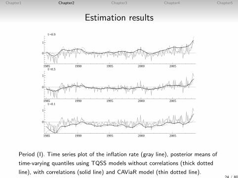
Period (I). Time series plot of the inflation rate (gray line), posterior means of
time-varying quantiles using TQSS models without correlations (thick dotted
line), with correlations (solid line) and CAViaR model (thin dotted line).24 / 80
Chapter1 Chapter2 Chapter3 Chapter4 Chapter5
Estimation results
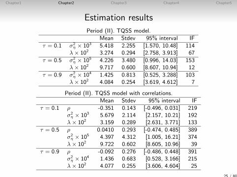
Period (II). TQSS model.Mean Stdev 95% interval IF
τ = 0.1 σ2η × 103 5.418 2.255 [1.570, 10.48] 114
λ× 102 3.274 0.294 [2.758, 3.913] 67
τ = 0.5 σ2η × 105 4.226 3.480 [0.996, 14.03] 153
λ× 102 9.717 0.600 [8.607, 10.94] 12
τ = 0.9 σ2η × 104 1.425 0.813 [0.525, 3.288] 103
λ× 102 4.084 0.254 [3.619, 4.612] 7
Period (II). TQSS model with correlations.Mean Stdev 95% interval IF
τ = 0.1 ρ -0.351 0.143 [-0.496, 0.031] 219σ2η × 103 5.679 2.114 [2.157, 10.21] 192
λ× 102 3.159 0.289 [2.631, 3.771] 133
τ = 0.5 ρ 0.0410 0.293 [-0.474, 0.485] 389σ2η × 105 4.397 4.312 [1.005, 16.21] 374
λ× 102 9.722 0.602 [8.605, 10.96] 39
τ = 0.9 ρ -0.092 0.276 [-0.486, 0.448] 391σ2η × 104 1.436 0.683 [0.528, 3.166] 215
λ× 102 4.077 0.255 [3.606, 4.604] 25
25 / 80
Chapter1 Chapter2 Chapter3 Chapter4 Chapter5
Estimation results
1985 1990 1995 2000 2005 2010
0
2
τ=0.9
1985 1990 1995 2000 2005 2010
0
2τ=0.5
1985 1990 1995 2000 2005 2010−2
0
2τ=0.1
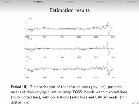
Period (II). Time series plot of the inflation rate (gray line), posterior
means of time-varying quantiles using TQSS models without correlations
(thick dotted line), with correlations (solid line) and CAViaR model (thin
dotted line). 26 / 80
Chapter1 Chapter2 Chapter3 Chapter4 Chapter5
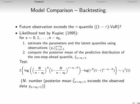
Model Comparison – Backtesting.
• Future observation exceeds the τ -quantile ((1− τ)-VaR)?
• Likelihood test by Kupiec (1995):for s = 0, 1, . . . , n − n0,
1. estimate the parameters and the latent quantiles usingobservations yts+n0
t=s+1
2. compute the posterior mean of the predictive distribution ofthe one-step-ahead quantile, ξs+n0+1.
Test:
2
log
(( N
n − n0
)N(1− N
n − n0
)n−n0−N)−log(τN(1−τ)n−n0−N)
∼ χ2(1)
(N: number (posterior mean ξs+n0+1 exceeds the observeddata ys+n0+1))
27 / 80
Chapter1 Chapter2 Chapter3 Chapter4 Chapter5
Model Comparison – Backtesting.
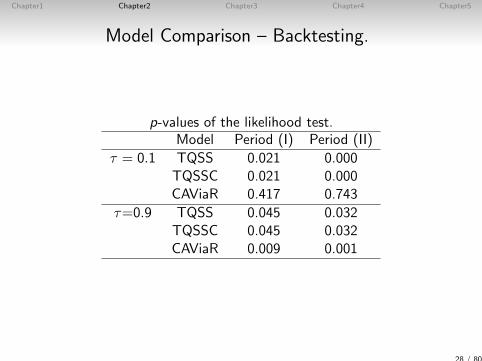
p-values of the likelihood test.Model Period (I) Period (II)
τ = 0.1 TQSS 0.021 0.000TQSSC 0.021 0.000CAViaR 0.417 0.743
τ=0.9 TQSS 0.045 0.032TQSSC 0.045 0.032CAViaR 0.009 0.001
28 / 80
Chapter1 Chapter2 Chapter3 Chapter4 Chapter5
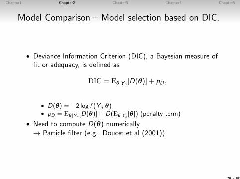
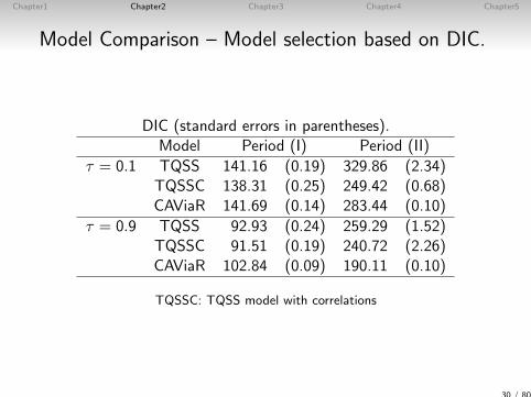
Model Comparison – Model selection based on DIC.
• Deviance Information Criterion (DIC), a Bayesian measure offit or adequacy, is defined as
DIC = Eθ|Yn[D(θ)] + pD ,
• D(θ) = −2 log f (Yn|θ)• pD = Eθ|Yn
[D(θ)]− D(Eθ|Yn[θ]) (penalty term)
• Need to compute D(θ) numerically→ Particle filter (e.g., Doucet et al (2001))
29 / 80
Chapter1 Chapter2 Chapter3 Chapter4 Chapter5
Model Comparison – Model selection based on DIC.
DIC (standard errors in parentheses).Model Period (I) Period (II)
τ = 0.1 TQSS 141.16 (0.19) 329.86 (2.34)TQSSC 138.31 (0.25) 249.42 (0.68)CAViaR 141.69 (0.14) 283.44 (0.10)
τ = 0.9 TQSS 92.93 (0.24) 259.29 (1.52)TQSSC 91.51 (0.19) 240.72 (2.26)CAViaR 102.84 (0.09) 190.11 (0.10)
TQSSC: TQSS model with correlations
30 / 80
Chapter1 Chapter2 Chapter3 Chapter4 Chapter5
Conclusion
This study
• proposes a novel smoothing spline model for time-varyingquantiles.
• proposes the efficient MCMC algorithm using a normalvariance-mean mixture representation of the measurementerror term.
• extends the model to incorporate a correlation between thedependent variable and its one-step-ahead quantile.
• provides empirical analysis of Japanese inflation rate andconduct model comparison regarding both one-aheadpredictions and goodness-of-fit.
31 / 80
Chapter1 Chapter2 Chapter3 Chapter4 Chapter5
Chapter3
Dynamic equicorrelation stochastic volatility
32 / 80

Chapter1 Chapter2 Chapter3 Chapter4 Chapter5
Introduction
• Daily stock return data ...• (time-varying) correlations• volatility-clustering• leverage effect and cross leverage effect
⇒ stochastic volatility model
• Equicorrelation assumption ...• superior portfolio allocation results• reduced estimation noise
(Elton and Gruber (1973))DCC model (e.g., Engle and Kelly (2012))
33 / 80
Chapter1 Chapter2 Chapter3 Chapter4 Chapter5
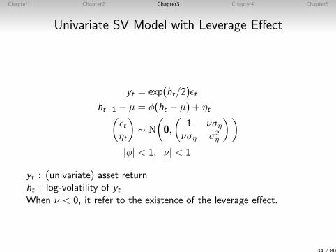
Univariate SV Model with Leverage Effect
yt = exp(ht/2)εt
ht+1 − µ = φ(ht − µ) + ηt(εtηt
)∼ N
(0,
(1 νση
νση σ2η
))|φ| < 1, |ν| < 1
yt : (univariate) asset returnht : log-volatility of ytWhen ν < 0, it refer to the existence of the leverage effect.
34 / 80
Chapter1 Chapter2 Chapter3 Chapter4 Chapter5
Equicorrelation Matrix
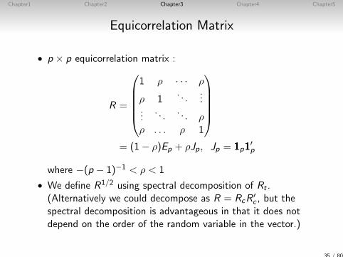
• p × p equicorrelation matrix :
R =
1 ρ · · · ρ
ρ 1. . .
......
. . .. . . ρ
ρ . . . ρ 1
= (1− ρ)Ep + ρJp, Jp = 1p1
′p
where −(p − 1)−1 < ρ < 1
• We define R1/2 using spectral decomposition of Rt .(Alternatively we could decompose as R = RcR
′c , but the
spectral decomposition is advantageous in that it does notdepend on the order of the random variable in the vector.)
35 / 80
Chapter1 Chapter2 Chapter3 Chapter4 Chapter5
MSV Model with DE and Cross Leverage
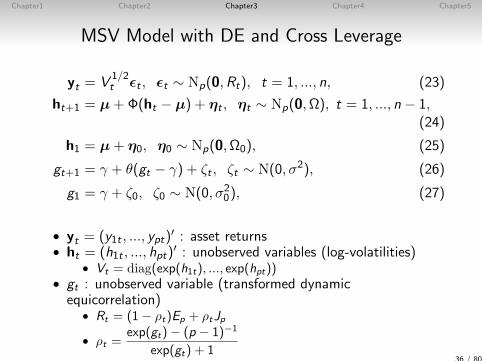
yt = V1/2t εt , εt ∼ Np(0,Rt), t = 1, ..., n, (23)
ht+1 = µ+Φ(ht − µ) + ηt , ηt ∼ Np(0,Ω), t = 1, ..., n − 1,(24)
h1 = µ+ η0, η0 ∼ Np(0,Ω0), (25)
gt+1 = γ + θ(gt − γ) + ζt , ζt ∼ N(0, σ2), (26)
g1 = γ + ζ0, ζ0 ∼ N(0, σ20), (27)
• yt = (y1t , ..., ypt)′ : asset returns
• ht = (h1t , ..., hpt)′ : unobserved variables (log-volatilities)
• Vt = diag(exp(h1t), ..., exp(hpt))• gt : unobserved variable (transformed dynamicequicorrelation)
• Rt = (1− ρt)Ep + ρtJp
• ρt =exp(gt)− (p − 1)−1
exp(gt) + 136 / 80
Chapter1 Chapter2 Chapter3 Chapter4 Chapter5
MSV Model with DE and Cross Leverage
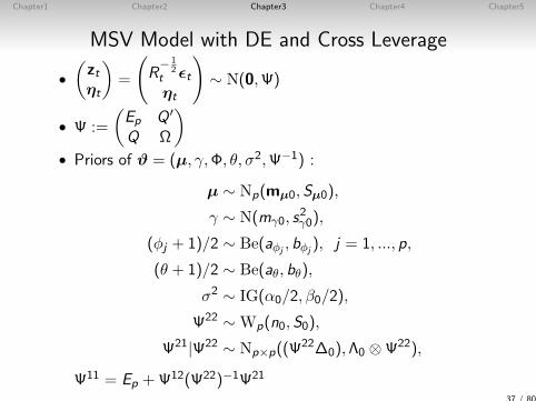
•(ztηt
)=
(R− 1
2t εtηt
)∼ N(0,Ψ)
• Ψ :=
(Ep Q ′
Q Ω
)• Priors of ϑ = (µ, γ,Φ, θ, σ2,Ψ−1) :
µ ∼ Np(mµ0,Sµ0),
γ ∼ N(mγ0, s2γ0),
(φj + 1)/2 ∼ Be(aφj, bφj
), j = 1, ..., p,
(θ + 1)/2 ∼ Be(aθ, bθ),
σ2 ∼ IG(α0/2, β0/2),
Ψ22 ∼ Wp(n0,S0),
Ψ21|Ψ22 ∼ Np×p((Ψ22∆0),Λ0 ⊗Ψ22),
Ψ11 = Ep +Ψ12(Ψ22)−1Ψ21
37 / 80
Chapter1 Chapter2 Chapter3 Chapter4 Chapter5
Bayesian Estimation
Posterior:
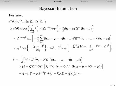
f (ϑ, htnt=1, gtnt=1|ytnt=1)
∝ π(ϑ)× exp
( n∑t=1
lt
)× |Ω0|−
12 exp
− 1
2(h1 − µ)′Ω−1
0 (h1 − µ)
× |Ω|−n−12 exp
[− 1
2
n−1∑t=1
ht+1 − µ− Φ(ht − µ)′Ω−1ht+1 − µ− Φ(ht − µ)]
× σ−10 exp
− (g1 − γ)2
2σ20
× (σ2)−
n−12 exp
[−∑n−1
t=1 gt+1 − (1− θ)γ − gt2
2σ2
],
lt = −1
2
[R
− 12
t V− 1
2t yt − Q ′
1Σ−1ht+1 − µ− Φ(ht − µ)
]′× (E − Q ′Ω−1Q)−1
[R
− 12
t V− 1
2t yt − Q ′Ω−1ht+1 − µ− Φ(ht − µ)
]− 1
2log(1− ρt)
p−1(1 + (p − 1)ρt) −1
2
∑pj=1 hjt .
38 / 80
Chapter1 Chapter2 Chapter3 Chapter4 Chapter5
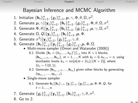
Bayesian Inference and MCMC Algorithm
1. Initialize htnt=1, gtnt=1,µ, γ,Φ, θ,Ω, σ2.
2. Generate µ, γ|ytnt=1, htnt=1, gtnt=1,Φ, θ,Ω, σ2.
3. Generate Φ, θ|ytnt=1, htnt=1, gtnt=1,µ, γ,Ω, σ2.
4. Generate Ω,Q|ytnt=1, htnt=1,µ,Φ.
5. Generate σ2|ytnt=1, gtnt=1, γ, θ.6. Generate htnt=1|ytnt=1, gtnt=1,µ,Φ,Ω.
• Multi-move sampler (Omori and Watanabe (2008))6.1 Divide ht = (h1t , ..., hpt)
′nt=1 into K + 1 blocks,(hkm−1+1, ..., hkm ), m = 1, ...,K with k0 = 0, kK+1 = n, usingstochastic knots km = int[n(m + Um)/(K + 2)], whereUm ∼ U(0, 1).
6.2 Generate (hkm−1+1, ..., hkm ) given other blocks by generating(ηkm−1 , ...,ηkm−1).
• Single-move sampler
6.1 Generate ht |hs−t , ytnt=1, gtnt=1,µ,Φ,Ψ,Q, fort = 1, ..., n.
7. Generate gtnt=1|ytnt=1, htnt=1, γ, θ, σ2.
8. Go to 2.39 / 80
Chapter1 Chapter2 Chapter3 Chapter4 Chapter5
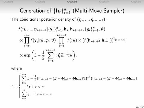
Generation of htnt=1 (Multi-Move Sampler)
The conditional posterior density of (ηs , ...,ηs+r−1) :
f (ηs , ...,ηs+r−1|ytnt=1,hs ,hs+r+1, gtnt=1,ϑ)
∝s+r∏t=s
f (yt |ht , gt ,ϑ)s+r−1∏t=s
f (ηt)× (f (hs+r+1|hs+r ))Is+r<n
∝ exp
(L− 1
2
s+r−1∑t=s
η′tΩ
−1ηt
),
where
L =
s+r∑t=s
lt −1
2hs+r+1 − (E − Φ)µ− Φhs+r′Ω−1hs+r+1 − (E − Φ)µ− Φhs+r
if s + r < n,n∑
t=s
lt if s + r = n,
40 / 80
Chapter1 Chapter2 Chapter3 Chapter4 Chapter5
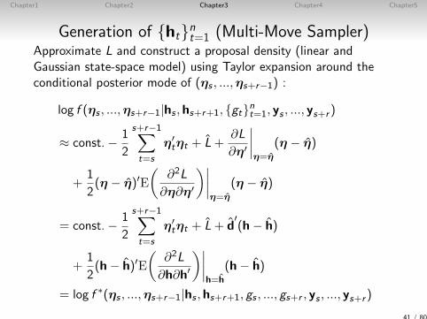
Generation of htnt=1 (Multi-Move Sampler)Approximate L and construct a proposal density (linear andGaussian state-space model) using Taylor expansion around theconditional posterior mode of (ηs , ...,ηs+r−1) :
log f (ηs , ...,ηs+r−1|hs ,hs+r+1, gtnt=1, ys , ..., ys+r )
≈ const.− 1
2
s+r−1∑t=s
η′tηt + L+
∂L
∂η′
∣∣∣∣η=η
(η − η)
+1
2(η − η)′E
(∂2L
∂η∂η′
)∣∣∣∣η=η
(η − η)
= const.− 1
2
s+r−1∑t=s
η′tηt + L+ d
′(h− h)
+1
2(h− h)′E
(∂2L
∂h∂h′
)∣∣∣∣h=h
(h− h)
= log f ∗(ηs , ...,ηs+r−1|hs ,hs+r+1, gs , ..., gs+r , ys , ..., ys+r )
41 / 80
Chapter1 Chapter2 Chapter3 Chapter4 Chapter5
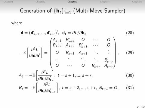
Generation of htnt=1 (Multi-Move Sampler)
where
d = (d′s+1, ...,d′s+r )
′, dt = ∂L/∂ht (28)
−E
[∂2L
∂h∂h′
]=
As+1 B ′
s+2 O · · · OBs+2 As+2 B ′
s+3 · · · O
O Bs+3 As+3. . .
......
. . .. . .
. . . B ′s+r
O · · · O Bs+r As+r
, (29)
At = −E
[∂2L
∂ht∂h′t
], t = s + 1, ..., s + r , (30)
Bt = −E
[∂2L
∂ht∂h′t−1
], t = s + 2, ..., s + r , Bs+1 = O. (31)
42 / 80
Chapter1 Chapter2 Chapter3 Chapter4 Chapter5
Generation of htnt=1 (Multi-Move Sampler)
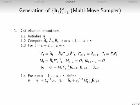
1. Disturbance smoother:
1.1 Initialize η1.2 Compute dt , At , Bt , t = s + 1, ..., s + r1.3 For t = s + 2, ..., s + r ,
Ct = At − BtC−1t−1B
′t , Cs+1 = As+1, Ct = FtF
′t
Mt = BtF′−1t−1, Ms+1 = O, Ms+r+1 = O
bt = dt −MtF−1t−1bt−1, bs+1 = ds+1
1.4 For t = s + 1, ..., s + r , defineyt = γt + C−1
t bt , γt = ht + F ′−1t M ′
t+1ht+1
43 / 80
Chapter1 Chapter2 Chapter3 Chapter4 Chapter5
Generation of htnt=1 (Multi-Move Sampler)
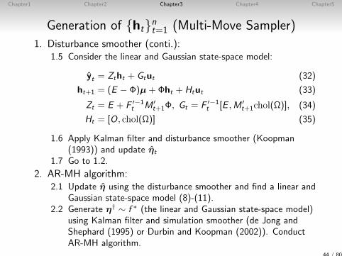
1. Disturbance smoother (conti.):1.5 Consider the linear and Gaussian state-space model:
yt = Ztht + Gtut (32)
ht+1 = (E − Φ)µ+Φht + Htut (33)
Zt = E + F ′−1t M ′
t+1Φ, Gt = F ′−1t [E ,M ′
t+1chol(Ω)], (34)
Ht = [O, chol(Ω)] (35)
1.6 Apply Kalman filter and disturbance smoother (Koopman(1993)) and update ηt
1.7 Go to 1.2.
2. AR-MH algorithm:2.1 Update η using the disturbance smoother and find a linear and
Gaussian state-space model (8)-(11).2.2 Generate η† ∼ f ∗ (the linear and Gaussian state-space model)
using Kalman filter and simulation smoother (de Jong andShephard (1995) or Durbin and Koopman (2002)). ConductAR-MH algorithm.
44 / 80
Chapter1 Chapter2 Chapter3 Chapter4 Chapter5
Generation of htnt=1 (Single-Move Sampler)
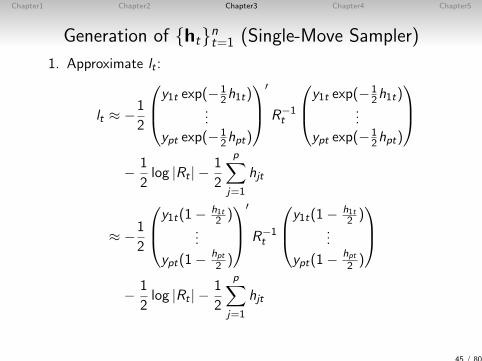
1. Approximate lt :
lt ≈ −1
2
y1t exp(−12h1t)
...ypt exp(−1
2hpt)
′
R−1t
y1t exp(−12h1t)
...ypt exp(−1
2hpt)
− 1
2log |Rt | −
1
2
p∑j=1
hjt
≈ −1
2
y1t(1− h1t2 )
...
ypt(1− hpt2 )
′
R−1t
y1t(1− h1t2 )
...
ypt(1− hpt2 )
− 1
2log |Rt | −
1
2
p∑j=1
hjt
45 / 80
Chapter1 Chapter2 Chapter3 Chapter4 Chapter5
Generation of htnt=1 (Single-Move Sampler)
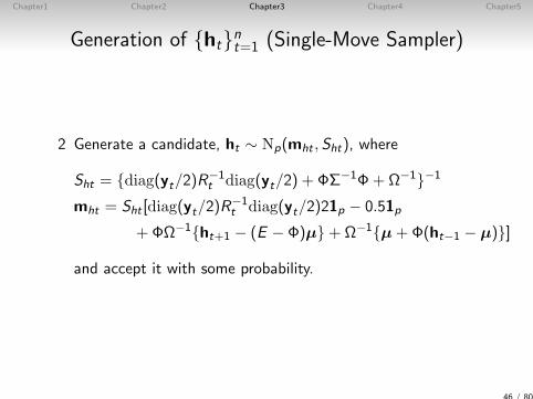
2 Generate a candidate, ht ∼ Np(mht ,Sht), where
Sht = diag(yt/2)R−1t diag(yt/2) + ΦΣ−1Φ+ Ω−1−1
mht = Sht [diag(yt/2)R−1t diag(yt/2)21p − 0.51p
+ΦΩ−1ht+1 − (E − Φ)µ+Ω−1µ+Φ(ht−1 − µ)]
and accept it with some probability.
46 / 80
Chapter1 Chapter2 Chapter3 Chapter4 Chapter5
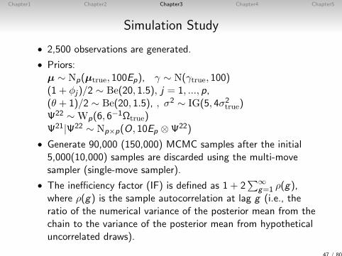
Simulation Study
• 2,500 observations are generated.
• Priors:µ ∼ Np(µtrue, 100Ep), γ ∼ N(γtrue, 100)(1 + φj)/2 ∼ Be(20, 1.5), j = 1, ..., p,(θ + 1)/2 ∼ Be(20, 1.5), , σ2 ∼ IG(5, 4σ2
true)Ψ22 ∼ Wp(6, 6
−1Ωtrue)Ψ21|Ψ22 ∼ Np×p(O, 10Ep ⊗Ψ22)
• Generate 90,000 (150,000) MCMC samples after the initial5,000(10,000) samples are discarded using the multi-movesampler (single-move sampler).
• The inefficiency factor (IF) is defined as 1 + 2∑∞
g=1 ρ(g),where ρ(g) is the sample autocorrelation at lag g (i.e., theratio of the numerical variance of the posterior mean from thechain to the variance of the posterior mean from hypotheticaluncorrelated draws).
47 / 80
Chapter1 Chapter2 Chapter3 Chapter4 Chapter5
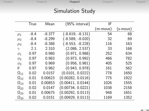
Simulation Study
True Mean (95% interval) IF(m-move) (s-move)
µ1 -8.4 -8.377 (-8.619, -8.131) 54 68µ2 -8.4 -8.299 (-8.589, -8.020) 32 69µ3 -8.4 -8.388 (-8.553, -8.228) 116 163γ 2.1 2.310 (2.086, 2.537) 33 168φ1 0.97 0.980 (0.971, 0.988) 252 634φ2 0.97 0.983 (0.973, 0.992) 466 782φ3 0.97 0.969 (0.956, 0.981) 405 525θ 0.97 0.962 (0.943, 0.978) 161 562Ω11 0.02 0.0157 (0.0101, 0.0222) 778 1650Ω12 0.01 0.00623 (0.00282, 0.0116) 775 1922Ω13 0.01 0.00853 (0.00411, 0.0144) 1026 1555Ω22 0.02 0.0147 (0.00734, 0.0221) 1038 2158Ω23 0.01 0.00675 (0.00292, 0.0113) 948 1651Ω33 0.02 0.0151 (0.00929, 0.0113) 1169 1352
48 / 80
Chapter1 Chapter2 Chapter3 Chapter4 Chapter5
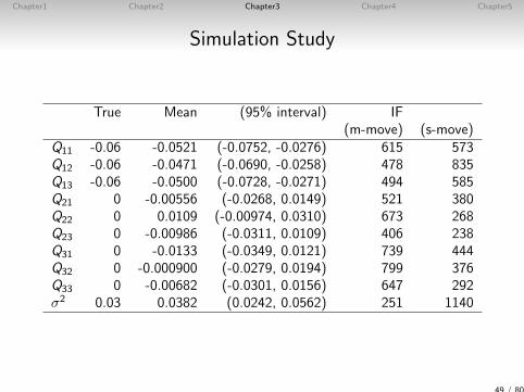
Simulation Study
True Mean (95% interval) IF(m-move) (s-move)
Q11 -0.06 -0.0521 (-0.0752, -0.0276) 615 573Q12 -0.06 -0.0471 (-0.0690, -0.0258) 478 835Q13 -0.06 -0.0500 (-0.0728, -0.0271) 494 585Q21 0 -0.00556 (-0.0268, 0.0149) 521 380Q22 0 0.0109 (-0.00974, 0.0310) 673 268Q23 0 -0.00986 (-0.0311, 0.0109) 406 238Q31 0 -0.0133 (-0.0349, 0.0121) 739 444Q32 0 -0.000900 (-0.0279, 0.0194) 799 376Q33 0 -0.00682 (-0.0301, 0.0156) 647 292σ2 0.03 0.0382 (0.0242, 0.0562) 251 1140
49 / 80
Chapter1 Chapter2 Chapter3 Chapter4 Chapter5
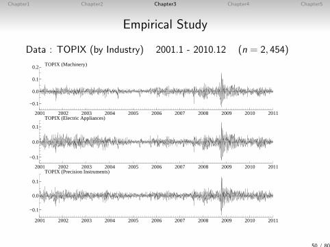
Empirical Study
Data : TOPIX (by Industry) 2001.1 - 2010.12 (n = 2, 454)
2001 2002 2003 2004 2005 2006 2007 2008 2009 2010 2011
−0.1
0.0
0.1
0.2 TOPIX (Machinery)
2001 2002 2003 2004 2005 2006 2007 2008 2009 2010 2011
−0.1
0.0
0.1
TOPIX (Electric Appliances)
2001 2002 2003 2004 2005 2006 2007 2008 2009 2010 2011
−0.1
0.0
0.1
TOPIX (Precision Instruments)
50 / 80
Chapter1 Chapter2 Chapter3 Chapter4 Chapter5
Empirical Study
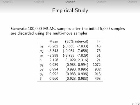
Generate 100,000 MCMC samples after the initial 5,000 samplesare discarded using the multi-move sampler.
Mean (95% interval) IFµ1 -8.262 (-8.660, -7.833) 43µ2 -8.343 (-9.054, -7.656) 76µ3 -8.298 (-8.739, -7.829) 51γ 2.126 (1.929, 2.316) 21φ1 0.989 (0.983, 0.994) 1072φ2 0.994 (0.990, 0.996) 902φ3 0.992 (0.988, 0.996) 913θ 0.960 (0.928, 0.983) 498
51 / 80
Chapter1 Chapter2 Chapter3 Chapter4 Chapter5
Empirical Study
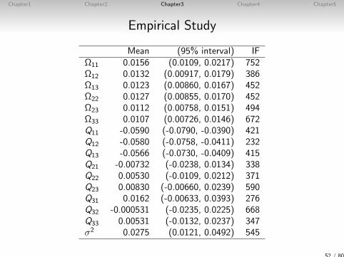
Mean (95% interval) IFΩ11 0.0156 (0.0109, 0.0217) 752Ω12 0.0132 (0.00917, 0.0179) 386Ω13 0.0123 (0.00860, 0.0167) 452Ω22 0.0127 (0.00855, 0.0170) 452Ω23 0.0112 (0.00758, 0.0151) 494Ω33 0.0107 (0.00726, 0.0146) 672Q11 -0.0590 (-0.0790, -0.0390) 421Q12 -0.0580 (-0.0758, -0.0411) 232Q13 -0.0566 (-0.0730, -0.0409) 415Q21 -0.00732 (-0.0238, 0.0134) 338Q22 0.00530 (-0.0109, 0.0212) 371Q23 0.00830 (-0.00660, 0.0239) 590Q31 0.0162 (-0.00633, 0.0393) 276Q32 -0.000531 (-0.0235, 0.0225) 668Q33 0.00531 (-0.0132, 0.0237) 347σ2 0.0275 (0.0121, 0.0492) 545
52 / 80
Chapter1 Chapter2 Chapter3 Chapter4 Chapter5
Empirical Study
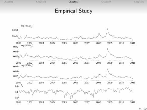
2001 2002 2003 2004 2005 2006 2007 2008 2009 2010 2011
0.025
0.050
exp(0.5 h1t)
2001 2002 2003 2004 2005 2006 2007 2008 2009 2010 2011
0.02
0.04
0.06 exp(0.5 h2t)
2001 2002 2003 2004 2005 2006 2007 2008 2009 2010 2011
0.02
0.04
0.06 exp(0.5 h3t)
2001 2002 2003 2004 2005 2006 2007 2008 2009 2010 2011
0.6
0.8
1.0 ρt
53 / 80
Chapter1 Chapter2 Chapter3 Chapter4 Chapter5
Empirical Study
2005 2010
−0.5
−0.4
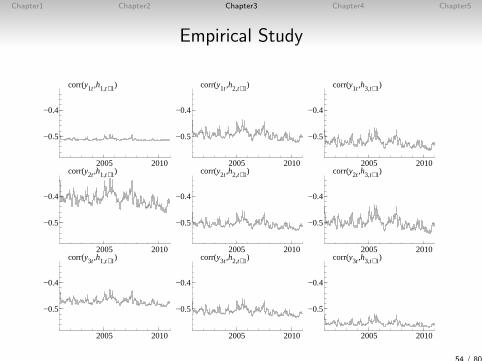
corr(y1t ,h1,t+1)
2005 2010
−0.5
−0.4
corr(y1t ,h2,t+1)
2005 2010
−0.5
−0.4
corr(y1t ,h3,t+1)
2005 2010
−0.5
−0.4
corr(y2t ,h1,t+1)
2005 2010
−0.5
−0.4
corr(y2t ,h2,t+1)
2005 2010
−0.5
−0.4
corr(y2t ,h3,t+1)
2005 2010
−0.5
−0.4
corr(y3t ,h1,t+1)
2005 2010
−0.5
−0.4
corr(y3t ,h2,t+1)
2005 2010
−0.5
−0.4
corr(y3t ,h3,t+1)
54 / 80
Chapter1 Chapter2 Chapter3 Chapter4 Chapter5
Summary
This study
• proposes the MSV model with dynamic equicorrelation andcross leverage
• proposes the efficient MCMC sampling algorithm
• provides empirical study using daily stock return data.
55 / 80

Chapter1 Chapter2 Chapter3 Chapter4 Chapter5
Chapter4
Realized stochastic volatility with dynamicequicorrelation and cross leverage
56 / 80

Chapter1 Chapter2 Chapter3 Chapter4 Chapter5
Introduction
• Realized measure has become available such as realizedvolatility by using high-frequency data (early studies are, e.g.,Andersen and Bollerslev (1998), Bandorff-Nielsen andShephard (2001)) in financial markets.
• Daily realized measures have some problems in the realmarkets and we should not regard such measures as therequired estimates (e.g., Hansen and Lunde (2006)).
• Why?The two major problems are:
1. market microstructure noise(caused mainly by (i) the presence of bid-ask spread, (ii)discrete trading and (iii) price adjustment)
2. non-trading hours
57 / 80
Chapter1 Chapter2 Chapter3 Chapter4 Chapter5
Introduction• On the other hand, the daily returns are not heavily affectedby such noise.
• The daily returns may provide us additional information toeliminate the bias
• Takahashi et al (2009) extend the univariate stochasticvolatility (SV) model and Realized stochastic volatility modelor RSV model.
• We extends the RSV model to the multivariate model byincorporating (1) the time-varying correlations between dailyreturns, (2) leverage effects and cross leverage effects (3)dynamic equicorrelation structure
• Realized covariance matrix : defined as the sum of the outerproduct of intraday returns over a specified period.
• Bandorff-Nielsen and Shephard (2004) show that it is aconsistent estimator of the quadratic cross-variance ofmultivariate log-price process with no microstructure noise.
• We obtain the realized variances and the realizedequicorrelation
58 / 80
Chapter1 Chapter2 Chapter3 Chapter4 Chapter5
Multivariate realized SV model with dynamicequicorrelation
• yt = (y1t , . . . , ypt)′: asset return vector
• xt = (x1t , . . . , xpt)′: vector of the logarithm of the
corresponding realized variances
• RCor t : the realized correlation matrix corresponding to yt• Define
x∗t = log
(p − 1)−1 + ρ∗t
1− ρ∗t
, ρ∗t =
2
p(p − 1)
∑j1<j2
(RCor t)j1j2 ,
as the transformed realized equicorrelation.
59 / 80
Chapter1 Chapter2 Chapter3 Chapter4 Chapter5
Multivariate realized SV model with dynamicequicorrelation
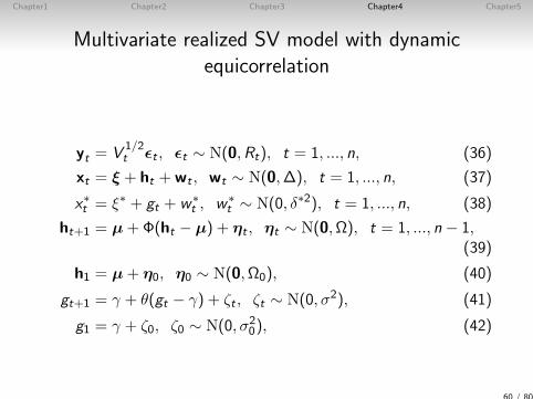
yt = V1/2t εt , εt ∼ N(0,Rt), t = 1, ..., n, (36)
xt = ξ + ht +wt , wt ∼ N(0,∆), t = 1, ..., n, (37)
x∗t = ξ∗ + gt + w∗t , w∗
t ∼ N(0, δ∗2), t = 1, ..., n, (38)
ht+1 = µ+Φ(ht − µ) + ηt , ηt ∼ N(0,Ω), t = 1, ..., n − 1,(39)
h1 = µ+ η0, η0 ∼ N(0,Ω0), (40)
gt+1 = γ + θ(gt − γ) + ζt , ζt ∼ N(0, σ2), (41)
g1 = γ + ζ0, ζ0 ∼ N(0, σ20), (42)
60 / 80
Chapter1 Chapter2 Chapter3 Chapter4 Chapter5
Multivariate realized SV model with dynamicequicorrelation
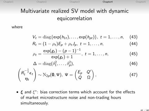
where
Vt = diagexp(h1t), . . . , exp(hpt), t = 1, . . . , n, (43)
Rt = (1− ρt)Ep + ρtJp, t = 1, . . . , n, (44)
ρt =exp(gt)− (p − 1)−1
exp(gt) + 1, t = 1, . . . , n, (45)
∆ = diag(δ21 , . . . , δ2p), (46)(
R− 1
2t εtηt
)∼ N2p(0,Ψ), Ψ =
(Ep Q ′
Q Ω
), (47)
• ξ and ξ∗: bias correction terms which account for the effectsof market microstructure noise and non-trading hourssimultaneously.
61 / 80
Chapter1 Chapter2 Chapter3 Chapter4 Chapter5
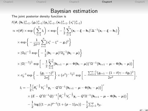
Bayesian estimationThe joint posterior density function is
f (ϑ, htnt=1, gtnt=1|ytnt=1, xtnt=1, x∗t nt=1)
∝ π(ϑ)× exp
( n∑t=1
lt
)× exp
−
1
2
n∑t=1
(xt − ξ − ht)′∆−1(xt − ξ − ht)
× exp
−
1
2δ∗2
n∑t=1
(x∗t − ξ∗ − gt)2
× |Ω0|−12 exp
−
1
2(h1 − µ)′Ω−1
0 (h1 − µ)
× |Ω|−n−12 exp
[−
1
2
n−1∑t=1
ht+1 − µ− Φ(ht − µ)′Ω−1ht+1 − µ− Φ(ht − µ)]
× σ−10 exp
−
(g1 − γ)2
2σ20
× (σ2)−
n−12 exp
[−
∑n−1t=1 gt+1 − (1− θ)γ − θgt2
2σ2
],
lt = −1
2
[R
− 12
t V− 1
2t yt − Q′Ω−1ht+1 − µ− Φ(ht − µ)
]′× (E − Q′Ω−1Q)−1
[R
− 12
t V− 1
2t yt − Q′Ω−1ht+1 − µ− Φ(ht − µ)
]−
1
2log(1− ρt)
p−1(1 + (p − 1)ρt) −1
2
∑pj=1 hjt .
62 / 80
Chapter1 Chapter2 Chapter3 Chapter4 Chapter5
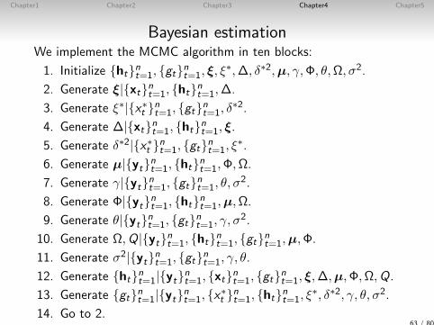
Bayesian estimationWe implement the MCMC algorithm in ten blocks:
1. Initialize htnt=1, gtnt=1, ξ, ξ∗,∆, δ∗2,µ, γ,Φ, θ,Ω, σ2.
2. Generate ξ|xtnt=1, htnt=1,∆.
3. Generate ξ∗|x∗t nt=1, gtnt=1, δ∗2.
4. Generate ∆|xtnt=1, htnt=1, ξ.
5. Generate δ∗2|x∗t nt=1, gtnt=1, ξ∗.
6. Generate µ|ytnt=1, htnt=1,Φ,Ω.
7. Generate γ|ytnt=1, gtnt=1, θ, σ2.
8. Generate Φ|ytnt=1, htnt=1,µ,Ω.
9. Generate θ|ytnt=1, gtnt=1, γ, σ2.
10. Generate Ω,Q|ytnt=1, htnt=1, gtnt=1,µ,Φ.
11. Generate σ2|ytnt=1, gtnt=1, γ, θ.
12. Generate htnt=1|ytnt=1, xtnt=1, gtnt=1, ξ,∆,µ,Φ,Ω,Q.
13. Generate gtnt=1|ytnt=1, x∗t nt=1, htnt=1, ξ∗, δ∗2, γ, θ, σ2.
14. Go to 2.63 / 80
Chapter1 Chapter2 Chapter3 Chapter4 Chapter5
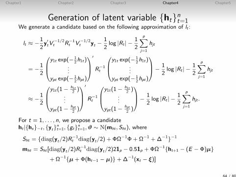
Generation of latent variable htnt=1We generate a candidate based on the following approximation of lt :
lt ≈ −1
2y′tV
−1/2t R−1
t V−1/2t yt −
1
2log |Rt | −
1
2
p∑j=1
hjt
= −1
2
y1t exp(− 12h1t)
...ypt exp(− 1
2hpt)
′
R−1t
y1t exp(− 12h1t)
...ypt exp(− 1
2hpt)
− 1
2log |Rt | −
1
2
p∑j=1
hjt
≈ −1
2
y1t(1− h1t2)
...
ypt(1− hpt2)
′
R−1t
y1t(1− h1t2)
...
ypt(1− hpt2)
− 1
2log |Rt | −
1
2
p∑j=1
hjt .
For t = 1, . . . , n, we propose a candidateht |hs−t , ytnt=1, gtnt=1,ϑ ∼ N(mht , Sht), where
Sht = diag(yt/2)R−1t diag(yt/2) + ΦΩ−1Φ+ Ω−1 +∆−1−1
mht = Sht [diag(yt/2)R−1t diag(yt/2)21p − 0.51p +ΦΩ−1ht+1 − (E − Φ)µ
+Ω−1µ+Φ(ht−1 − µ)+∆−1(xt − ξ)]
64 / 80
Chapter1 Chapter2 Chapter3 Chapter4 Chapter5
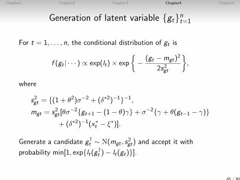
Generation of latent variable gtnt=1
For t = 1, . . . , n, the conditional distribution of gt is
f (gt | · · · ) ∝ exp(lt)× exp
− (gt −mgt)
2
2s2gt
,
where
s2gt = (1 + θ2)σ−2 + (δ∗2)−1−1,
mgt = s2gt [θσ−2gt+1 − (1− θ)γ+ σ−2γ + θ(gt−1 − γ)
+ (δ∗2)−1(x∗t − ξ∗)].
Generate a candidate g †t ∼ N(mgt , s
2gt) and accept it with
probability min[1, explt(g †t )− lt(gt)].
65 / 80
Chapter1 Chapter2 Chapter3 Chapter4 Chapter5
Illustrative example using simulated data
• We generate 2,500 observations (n = 2500).
• Using the single-move sampler, we generate 100,000 MCMCsamples after discarding the first 10,000 samples as theburn-in period.
66 / 80
Chapter1 Chapter2 Chapter3 Chapter4 Chapter5
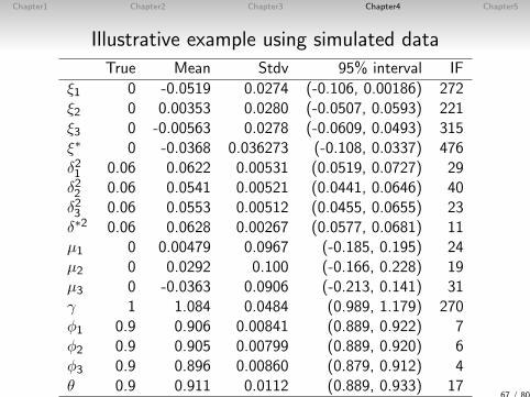
Illustrative example using simulated data
True Mean Stdv 95% interval IF
ξ1 0 -0.0519 0.0274 (-0.106, 0.00186) 272ξ2 0 0.00353 0.0280 (-0.0507, 0.0593) 221ξ3 0 -0.00563 0.0278 (-0.0609, 0.0493) 315ξ∗ 0 -0.0368 0.036273 (-0.108, 0.0337) 476δ21 0.06 0.0622 0.00531 (0.0519, 0.0727) 29δ22 0.06 0.0541 0.00521 (0.0441, 0.0646) 40δ23 0.06 0.0553 0.00512 (0.0455, 0.0655) 23δ∗2 0.06 0.0628 0.00267 (0.0577, 0.0681) 11µ1 0 0.00479 0.0967 (-0.185, 0.195) 24µ2 0 0.0292 0.100 (-0.166, 0.228) 19µ3 0 -0.0363 0.0906 (-0.213, 0.141) 31γ 1 1.084 0.0484 (0.989, 1.179) 270φ1 0.9 0.906 0.00841 (0.889, 0.922) 7φ2 0.9 0.905 0.00799 (0.889, 0.920) 6φ3 0.9 0.896 0.00860 (0.879, 0.912) 4θ 0.9 0.911 0.0112 (0.889, 0.933) 17
67 / 80
Chapter1 Chapter2 Chapter3 Chapter4 Chapter5
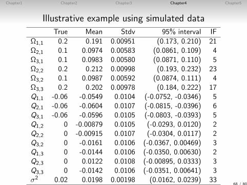
Illustrative example using simulated data
True Mean Stdv 95% interval IF
Ω1,1 0.2 0.191 0.00951 (0.173, 0.210) 21Ω2,1 0.1 0.0974 0.00583 (0.0861, 0.109) 4Ω3,1 0.1 0.0983 0.00580 (0.0871, 0.110) 5Ω2,2 0.2 0.212 0.00998 (0.193, 0.232) 23Ω3,2 0.1 0.0987 0.00592 (0.0874, 0.111) 4Ω3,3 0.2 0.202 0.00978 (0.184, 0.222) 17Q1,1 -0.06 -0.0549 0.0104 (-0.0752, -0.0346) 5Q2,1 -0.06 -0.0604 0.0107 (-0.0815, -0.0396) 6Q3,1 -0.06 -0.0596 0.0105 (-0.0803, -0.0393) 5Q1,2 0 -0.00879 0.0105 (-0.0293, 0.0120) 2Q2,2 0 -0.00915 0.0107 (-0.0304, 0.0117) 2Q3,2 0 -0.0161 0.0106 (-0.0367, 0.00469) 3Q1,3 0 -0.0144 0.0106 (-0.0350, 0.00630) 2Q2,3 0 0.0122 0.0108 (-0.00895, 0.0333) 3Q3,3 0 -0.0142 0.0106 (-0.0351, 0.00641) 3σ2 0.02 0.0198 0.00198 (0.0162, 0.0239) 33
68 / 80
Chapter1 Chapter2 Chapter3 Chapter4 Chapter5
Empirical study
• The daily close-to-close stock return and realized measuredata of: (1) Bank of America (BAC), (2) JP Morgan (JPM),(3) International Business Machines (IBM), (4) Microsoft(MSFT), (5) Exxon Mobil (XOM), (6) Alcoa (AA), (7)American Express (AXP), (8) Du Pont (DD), (9) GeneralElectric (GE) and (10) Coca Cola (KO).
• The sample period : February 1, 2001 - December 31, 2009(2228 observations)
69 / 80

Chapter1 Chapter2 Chapter3 Chapter4 Chapter5
Chapter5
Dynamic block-equicorrelation, realized stochasticvolatility and cross leverage
70 / 80
Chapter1 Chapter2 Chapter3 Chapter4 Chapter5
Introduction
• Dynamic equicorrelation assumption : too strong and runscounter to the intuition?
• The general model that all correlations between thedependent variables are not equal but time-varying: difficultto estimate / overfitting to the past data
• We introduce the multivariate RSV model with dynamic“block-equicorrelation” and cross leverage effect.(intermediate generalization of the model in Chapter 4)
• It is difficult to keep the block-equicorrelation matricespositive definite since we cannot define the support of thedynamic equicorrelation factors analytically.→ Required to use the realized measures.
71 / 80

Chapter1 Chapter2 Chapter3 Chapter4 Chapter5
Block-equicorrelation matrixSuppose that a random variable vector has a block equicorrelationstructure where the correlation matrix takes the form
R =
(1 − ρ11)Ep1 + ρ111p1 1′p1
ρ121p1 1′p2
· · · ρ1d1p1 1′pd
ρ121p2 1′p1
(1 − ρ22)Ep2 + ρ221p2 1′p2
. . ....
.
.
.. . .
. . . ρd−1,d1pd−11′pd
ρ1d1pd 1′p1
· · · ρd−1,d1pd 1′pd−1
(1 − ρdd )Epd + ρdd1pd 1′pd
The determinant is given by
|R| =d∏
l=1
(1− ρll)pl−1|RA + RBP|,
where
RA = diag(1− ρ11, . . . , 1− ρdd),
RB =
ρ11 · · · ρ1d...
. . ....
ρ1d · · · ρdd
, P = diag(p1, . . . , pd).
72 / 80
Chapter1 Chapter2 Chapter3 Chapter4 Chapter5
Block-equicorrelation matrix
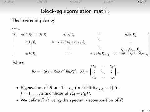
The inverse is given by
R−1 =
(1 − ρ11)−1Ep1 + r111p1 1
′p1
r121p1 1′p2
· · · r1d1p1 1′pd
r121p2 1′p1
(1 − ρ22)−1Ep2 + r221p2 1
′p2
. . ....
.
.
.. . .
. . . rd−1,d1pd−11′pd
r1d1pd 1′p1
· · · rd−1,d1pd 1′pd−1
(1 − ρdd )−1Epd + rdd1pd 1
′pd
,
where
RC = −(RA + RBP)−1RBR−1A , RC =
r11 · · · r1d...
. . ....
r1d · · · rdd
.
• Eigenvalues of R are 1− ρll (multiplicity pd − 1) forl = 1, . . . , d and those of RA + RBP.
• We define R1/2 using the spectral decomposition of R.
73 / 80
Chapter1 Chapter2 Chapter3 Chapter4 Chapter5
Multivariate realized SV model with dynamicblock-equicorrelation and cross leverage
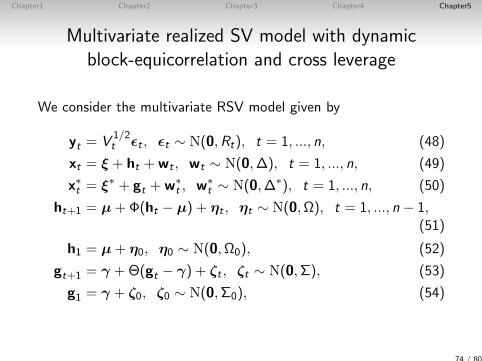
We consider the multivariate RSV model given by
yt = V1/2t εt , εt ∼ N(0,Rt), t = 1, ..., n, (48)
xt = ξ + ht +wt , wt ∼ N(0,∆), t = 1, ..., n, (49)
x∗t = ξ∗ + gt +w∗t , w∗
t ∼ N(0,∆∗), t = 1, ..., n, (50)
ht+1 = µ+Φ(ht − µ) + ηt , ηt ∼ N(0,Ω), t = 1, ..., n − 1,(51)
h1 = µ+ η0, η0 ∼ N(0,Ω0), (52)
gt+1 = γ +Θ(gt − γ) + ζt , ζt ∼ N(0,Σ), (53)
g1 = γ + ζ0, ζ0 ∼ N(0,Σ0), (54)
74 / 80
Chapter1 Chapter2 Chapter3 Chapter4 Chapter5
Multivariate realized SV model with dynamicblock-equicorrelation and cross leverage
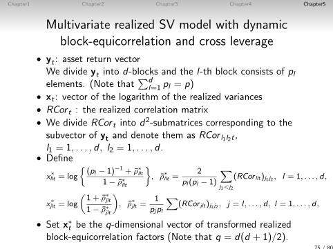
• yt : asset return vectorWe divide yt into d-blocks and the l-th block consists of plelements. (Note that
∑dl=1 pl = p)
• xt : vector of the logarithm of the realized variances• RCor t : the realized correlation matrix• We divide RCor t into d2-submatrices corresponding to thesubvector of yt and denote them as RCor l1l2t ,l1 = 1, . . . , d , l2 = 1, . . . , d .
• Define
x∗llt = log
(pl − 1)−1 + ρ∗llt
1− ρ∗llt
, ρ∗llt =
2
pl(pl − 1)
∑j1<j2
(RCor llt)j1j2 , l = 1, . . . , d ,
x∗jlt = log
(1 + ρ∗jlt1− ρ∗jlt
), ρ∗jlt =
1
pjpl
∑(RCor jlt)j1j2 , j = l , . . . , d , l = 1, . . . , d ,
• Set x∗t be the q-dimensional vector of transformed realizedblock-equicorrelation factors (Note that q = d(d + 1)/2).
75 / 80
Chapter1 Chapter2 Chapter3 Chapter4 Chapter5
Multivariate realized SV model with dynamicblock-equicorrelation and cross leverage
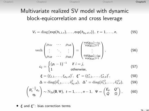
Vt = diagexp(h1,1,t), . . . , exp(hpd ,d,t), t = 1, . . . , n, (55)
vech
ρ11t · · · ρ1dt...
. . ....
ρ1dt · · · ρddt
=
exp(g11t )−c11exp(g11t )+1
...exp(gddt )−cddexp(gddt )+1
, (56)
cij =
(pi − 1)−1 if i = j ,
1 otherwise,(57)
ξ = (ξ1,1, . . . , ξpd ,d)′, ξ∗ = (ξ∗1,1, . . . , ξ
∗d,d)
′, (58)
∆ = diag(δ21,1, . . . , δ2pd ,d), ∆∗ = diag(δ∗21,1, . . . , δ
∗2d,d), (59)(
R− 1
2t εtηt
)∼ N2p(0,Ψ), t = 1, . . . , n − 1, Ψ =
(Ep Q ′
Q Ω
), (60)
• ξ and ξ∗: bias correction terms76 / 80
Chapter1 Chapter2 Chapter3 Chapter4 Chapter5
Bayesian estimation and MCMC algorithm
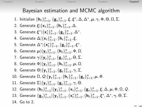
1. Initialize htnt=1, gtnt=1, ξ, ξ∗,∆,∆∗,µ,γ,Φ,Θ,Ω,Σ.
2. Generate ξ|xtnt=1, htnt=1,∆.
3. Generate ξ∗|x∗t nt=1, gtnt=1,∆∗.
4. Generate ∆|xtnt=1, htnt=1, ξ.
5. Generate ∆∗|x∗t nt=1, gtnt=1, ξ∗.
6. Generate µ|ytnt=1, htnt=1,Φ,Ω.
7. Generate γ|ytnt=1, gtnt=1,Θ,Σ.
8. Generate Φ|ytnt=1, htnt=1,µ,Ω.
9. Generate Θ|ytnt=1, gtnt=1,γ,Σ.
10. Generate Ω,Q|ytnt=1, htnt=1, gtnt=1,µ,Φ.
11. Generate Σ|ytnt=1, gtnt=1,γ,Θ.
12. Generate htnt=1|ytnt=1, xtnt=1, gtnt=1, ξ,∆,µ,Φ,Ω,Q.
13. Generate gtnt=1|ytnt=1, x∗t nt=1, htnt=1, ξ∗,∆∗,γ,Θ,Σ.
14. Go to 2.77 / 80
Chapter1 Chapter2 Chapter3 Chapter4 Chapter5
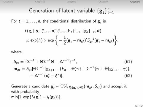
Generation of latent variable gtnt=1
For t = 1, . . . , n, the conditional distribution of gt is
f (gt |ytnt=1, x∗t nt=1, htnt=1, gt−t ,ϑ)
∝ exp(lt)× exp
− 1
2(gt −mgt)
′S−1gt (gt −mgt)
,
where
Sgt = Σ−1 +ΘΣ−1Θ+∆∗−1−1, (61)
mgt = Sgt [ΘΣ−1gt+1 − (Eq −Θ)γ+Σ−1γ +Θ(gt−1 − γ)+∆∗−1(x∗t − ξ∗)]. (62)
Generate a candidate g†t ∼ TNRt(gt)>0(mgt ,Sgt) and accept itwith probabilitymin[1, explt(g†t)− lt(gt)].
78 / 80
Chapter1 Chapter2 Chapter3 Chapter4 Chapter5
Generation of latent variable gtnt=1
Notice: the supports of gt , t = 1, . . . , n, are not expressedanalytically→ e.g., Random-walk MH algorithm with normal density cannotbe applied with ease because the normalizing constants ofq(gt , g
ct ) and q(gct , gt) are not equal.
In this case, the normalizing constants of q(gt , gct ) and q(gct , gt)
are coincided.
79 / 80

Chapter1 Chapter2 Chapter3 Chapter4 Chapter5
Empirical Study
• The daily close-to-close stock return and realized measuredata provided by Noureldin et al (2012)
• Group 1 (Finance):(1) Bank of America (BAC), (2) JP Morgan (JPM), (3)American Express (AXP),
• Group 2 (Information Technology and Others)(4) International Business Machines (IBM), (5) Microsoft(MSFT), (6) General Electric (GE),
• Group 3 (Materials)(7) Exxon Mobil (XOM), (8) Alcoa (AA), (9) Du Pont (DD).
• Three-block case (d = 3, q = 6) and each blocks consist ofthree components (p1 = p2 = p3 = 3, p = 9).
• The sample period : February 1, 2001 - December 31, 2009(2228 observations in total).
80 / 80


