
Michigan Technological UniversityDigital Commons @ Michigan
TechDissertations, Master's Theses and Master's Reports- Open Dissertations, Master's Theses and Master's Reports
2015
PETROPHYSICAL ANALYSIS AND ROCK-PHYSICS BASED PREDICTION OF SONICVELOCITIES IN CARBONATESYeliz EgemenMichigan Technological University
Copyright 2015 Yeliz Egemen
Follow this and additional works at: http://digitalcommons.mtu.edu/etds
Part of the Geophysics and Seismology Commons
Recommended CitationEgemen, Yeliz, "PETROPHYSICAL ANALYSIS AND ROCK-PHYSICS BASED PREDICTION OF SONIC VELOCITIES INCARBONATES", Master's Thesis, Michigan Technological University, 2015.http://digitalcommons.mtu.edu/etds/978

PETROPHYSICAL ANALYSIS AND ROCK-PHYSICS BASED PREDICTION OF SONIC VELOCITIES IN CARBONATES
By
Yeliz Egemen
A THESIS
Submitted in partial fulfillment of the requirements for the degree of
MASTER OF SCIENCE
In Geophysics
MICHIGAN TECHNOLOGICAL UNIVERSITY
2015
© 2015 Yeliz Egemen

This thesis has been approved in partial fulfillment of the requirements for the Degree of MASTER OF SCIENCE in Geophysics
Department of Geological and Mining Engineering and Sciences
Thesis Advisor: Dr. Wayne D. Pennington
Committee Member: Dr. Roger M. Turpening
Committee Member: Prof. Mir Sadri
Department Chair: Dr. John S. Gierke

iii
Table of Contents Acknowledgements ................................................................................................................ iv
Abstract ........................................................................................................................................ v
1 Introduction ........................................................................................................................ 1
2 Devonian System Geology .............................................................................................. 3
3 Methods ................................................................................................................................ 5
3.1 Picking Formation Tops .......................................................................................... 6
3.2 Petrophysical Analysis ............................................................................................ 8
3.3 Velocity Determinations ....................................................................................... 18
3.3.1 P-wave Velocity Determination from Wyllie’s Time-Average
Equation ............................................................................................................................ 18
3.3.2 S-wave Determination from Greenberg and Castagna ....................... 19
3.3.3 Velocity Determination from Rock Physics Modeling ........................ 20
3.4 Pore-type classification ........................................................................................ 30
4 Results & Discussion ...................................................................................................... 33
5 Conclusion ......................................................................................................................... 35
6 References ......................................................................................................................... 37
7 Appendices ........................................................................................................................ 39
7.1 Appendix (I): Crossplots ....................................................................................... 39
7.1.1 MID of DGA and UMA Crossplot .................................................................. 39
7.1.2 Additional Crossplots of Sampled Wells ................................................. 40
7.2 Appendix (II): Root-Mean-Square (RMS) Error Calculation .................... 51
7.3 Appendix (III): Lithology Log .............................................................................. 51
7.4 Appendix (IV): The Kuster-Toksöz Model (1974) ...................................... 53

iv
Acknowledgements First and foremost I would like to thanks to my advisor, Dr. Wayne D. Pennington. It was
his guidance, support, and expertise in geophysics that made my research and this paper
possible. Furthermore I would like to acknowledge the committee members in my
department, Professor Mir Sadri and Dr. Roger Turpening for their support and help.
I also want to recognize the team at Jason (now part of CGG) for the PowerLog software
they provided, enabling me to analyze the data necessary to complete my research.
Last but not least are my friends and family. Their support goes beyond words I can express
in this acknowledgment. My friends Evan Krettek, Qiang Guo, Lu Yang, Deniz Yener,
Fatmanur Karaman, Solmaz Hajmohammadi, Robert Richard and Paniz Khanmohammadi
Hazaveh have all helped me both personally and as a graduate student. My family, Selvin,
Yesim and Özdemir Egemen, played major roles in carrying me through tough times and
always pushing me to do my best.

v
Abstract
This study performs a petrophysical analysis and rock-physics modeling of the Traverse
Formation, using eleven different wells. In the first part of this study, well logs, crossplots,
and mineral identification were used to determine the rock components, lithology, and to
predict the sonic velocities of carbonate rocks using conventional methods for two of those
wells.
In the second part of this study, rock-physics modeling methods were used to predict the
sonic velocities using the Kuster-Toksöz equations. Sonic velocities are very difficult to
predict in carbonate rock because of their complex pore systems. To overcome this
difficulty, multiple aspect ratios for porosity were used to calculate sonic velocities for the
limestone, dolomite, quartz, anhydrite, and shale mixtures. Having determined the
lithology from conventional log analysis, the matrix moduli and densities were estimated.
Then the Kuster-Toksöz equations were used to calculate the elastic properties, using
different aspect ratios in an effort to obtain the best estimate for the observed P-wave
velocities, and to predict S-wave velocities (which had not been recorded), and compare
them with the predicted S-wave from Greenberg and Castagna equations.

1
1 Introduction Eleven wells were selected for this study, with appropriate logs covering the Traverse
Group Formation in the Michigan Basin, a Middle Devonian carbonate consisting of
calcite, dolomite, quartz, anhydrite and shale (Huntoon and Wylie, 2003).
This study attempts to use conventional logs in order to estimate sonic-log values.
Carbonate rocks are particularly challenging for such estimates due to the variety and
complexity of pore shapes (Xu and Payne, 2009). It is hoped that, through a systematic
approach of pore-shape analysis for different mineralogy as determined from conventional
logs, improved relations for sonic properties could be obtained. The conventional logs
include density (RHOB), neutron-porosity (NPHI, recorded on a limestone scale), gamma-
ray (GR), and photo-electric effect (PEF). Four different mineral components were found
to occur in the Traverse formation: calcite, dolomite, anhydrite, and quartz. Crossplots of
these four logs were used to identify those minerals.
Many empirical relations exist for the prediction of sonic velocities from other information,
such as porosity and matrix lithology. These have limited accuracy, and are particularly
problematic in carbonate rocks. Sonic velocities depend on many factors other than simple
porosity and lithology, including pore type. The Kuster-Toksöz (Kuster and Toksöz, 1974)
method assumes that pores can be approximated as penny-shaped ellipsoids of revolution,
with aspect ratios representing ranging from fine crack-like pores (between 0.001-0.01) to
spherical pores (1.0). Different mineral assemblages tend to exhibit behavior representing
2
different pore aspect ratios. Other investigators have found certain aspect ratios to be
useful in single-lithology rocks (Brie, 1985), and combinations of aspect ratios for mixed
lithologies (Xu and White, 1995).
In this study, inspired by the mixed-lithology studies by Xu and White (1995) and Xu and
Payne (2009), a complex set of lithologies, including a calcite-quartz mixture, and a
dolomite-anhydrite mixture, are analyzed in a systematic manner in an attempt to predict
sonic velocities using lithology-dependent pore aspect ratios for the porosity. The first part
of this thesis includes a description of the lithology estimate using the eleven wells as
examples shown in Appendix 7.1.3. In the second part of this thesis, the Kuster-Toksöz
method is used to predict sonic velocities for mixtures found in some of the wells studied.

3
2 Devonian System Geology The formation used in this study is found in the Michigan Basin. The Michigan Basin is
bounded by the Kankakee Arch, Cincinnati Arch and Findlay Arch (Rupp, 1997). The
Devonian System in the Michigan Basin is composed of five formations: Antrim Shale,
Traverse Formation, Traverse Limestone, Bell Shale, and Dundee Formation (Lilienthal,
1974). Carbonate and clastic rocks constitute the system with shale in the upper section.
The series of intermixed carbonates and clastic rock are due to multiple regression and
transgression events in the Middle Devonian (Huntoon and Wylie, 2003).
The uppermost layer of the Devonian System is the Antrim Shale, a dark brown organic
shale with a high radioactive response on the gamma-ray log (Lilienthal, 1974; Pringle,
1937). The Antrim Shale has a thickness of 60 ft to 220 ft (Hasenmueller and Bassett,
1979).
The Traverse Formation, Traverse Limestone and Bell Shale make up the Traverse Group.
The Traverse Group has a thickness ranging from 80 ft to 900 ft (Huntoon and Wylie,
2003). Traverse Formation is the uppermost layer of the Traverse Group and is composed
of gray shale and limestone (Huntoon and Wylie, 2003). The underlying Traverse
Limestone is the important formation in this group and consists of dolomite, shale, and
anhydrite, with substantial production of gas and oil (Catacosinos et al., 1990). The lowest
part of the Traverse Group, the Bell Shale, is a fossiliferous gray shale with thickness of
about 80 ft (Huntoon and Wylie, 2003).

4
The Dundee Limestone underlies the Traverse Group, and is brown to gray limestone with
a thickness of 25 ft to 35 ft (Catacosinos et al., 1990; Lilienthal, 1974). If the Bell Shale is
not present, then the Dundee directly underlies the Traverse Limestone. This thesis is
concerned only with the Traverse Limestone.
5
3 Methods Conventional sonic-log prediction can be exemplified by application of a simple sonic-
porosity relationship. This will be applied to a few wells, and that prediction compared
with recorded sonic values. The technique does not vary with lithology, except for the
value of a matrix velocity.
In order to perform more complicated analytical techniques, the lithology of the formation
must be known. The eleven wells selected for this study were all logged with the
conventional suite of logs (GR, RHOB, NPHI, PEF). In addition, they all had a sonic (DT)
log, for comparison with predictions.
Conventional log analysis, including picking of formation tops and crossplot analysis,
serves to identify the lithologies to be studied in the Traverse Limestone. Simple
predictions of sonic velocity are performed, using conventional approaches. Finally, the
Kuster-Toksöz equations are used, with pore aspect ratios determined in a systematic
manner, to predict the sonic velocities.

6
3.1 Picking Formation Tops This thesis will focus on the Traverse Limestone of the Traverse Group, consisting
primarily of limestone, frequently with high dolomite and shale content. For the most part,
the Gamma Ray (GR) log was used to pick tops, since the formations all have distinct GR
signatures.
The Traverse Group directly underlies the Antrim Shale with its characteristic high
radioactivity (more than 150° API). The top of the Traverse Formation is picked where the
GR values suddenly drop below 100° API. The Traverse Formation typically has
decreasing GR values with increasing depth. The top of Traverse Limestone, below the
Traverse Formation, is identified when the GR log values become stable with depth. The
top of Bell Shale, beneath the Traverse Limestone, is identified at the depth where the GR
log values suddenly increase, but then remain stable with increasing depth. The Dundee
Limestone, with extremely low and stable GR values, directly underlies the Bell Shale. An
example of logs with the tops picked is provided in Figure 3.1.

7
Figure 3.1 An example of the gamma ray (GR), density (RHOB), sonic (DT) and neutron porosity (NPHI) logs, with the tops of the Antrim Shale, Traverse Formation, Traverse Limestone, Bell Shale and Dundee picked in the Consumers Power Co well. This log displays use the following convention: The first column lists the depth, in feet. The first log track includes the GR log in black, and include the caliper (CAL) in dashed grey. The second log track displays the RHOB (blue), NPHI (red), and DT (green) and PEF (black).

8
3.2 Petrophysical Analysis The important parameters that determine the sonic velocities are the mineral composition
of the rocks and the porosity type; these parameters were estimated with petrophysical
analysis. The gamma ray log was used to determine shale content. The density log, neutron
log, and photoelectric absorption factor log were used to detect porosity of the rock,
calculate the volumetric factor and composition of the other minerals.
Various crossplots which include the Neutron-Density crossplot, the Mineral Identification
(MID) of dry grain density (DGA) and photo-electric effect (UMA) crossplot and the
Density-Photoelectric Absorption (PEF) crossplot were used to determine lithology.
These will be described individually here, with display parameters used in all presentations.
This discussion begins with an example of a limestone containing some quartz, using the
Martin well and Kennedy wells. The other lithology, present deeper in these wells, consists
of dolomite and anhydrite, and will be discussed later using the Kennedy well. These two
wells are provided as examples, and the remaining nine wells are presented in an appendix.
The shallower portion of the Traverse Limestone in the Martin well, with logs and
crossplots displayed in Figures 3.2.1-4, presents a limestone with a significant amount of
quartz typical of many wells. Some parts of the formation also contain a significant amount
of clay, but for this example the depths containing clay will be ignored. The logs are
displayed in Figure 3.2.1, covering a large depth interval with a range of lithologies (clean
limestone shallower and more clay-rich or shalier deeper).

9
Figure 3.2.1. A log suite for Traverse Limestone in the Martin well, with depth in ft. In the first track, the red line is gamma-ray log, GR, and the grey line is the caliper log, CALI. In the second track the red line is the neutron log, NPHI, the blue line represents the density log, RHOB. Finally, in the third track the green line is the sonic log, DT, and the black line represents the photo-electric factor log, PEF. The various log scales are indicated in the track headers. (The depth range used for crossplots in Figures 3.2.2 -3.2.4 is 3150-3250 ft).
In all of the wells studied, combinations of four logs, the gamma ray log, density log,
neutron log, and photoelectric absorption factor log were used to identify the five mineral
components: quartz, calcite, dolomite and anhydrite (the fifth constraint is that the sum of
their components must equal one, a feature exploited by the crossplots). Figure 3.2.2 shows
a typical neutron-density crossplot, with the color axis showing shale content (from GR

10
log), over a depth range that includes the limestone with quartz (3150-3250 ft). This
crossplot suggests that in this well, the Traverse Limestone includes not only limestone,
but also a significant amount of quartz and a small amount of clay. The mineral
identification “MID” crossplot of UMA and DGA in Figure 3.2.3 uses dry grain density
(DGA or RHOMAND), determined from RHOB and NPHI, and the photo-electric effect
(UMA or UMAP), determined from PEF and RHOB, to help estimate the mineral
components. The RHOB-PEF crossplot shown in Figure 3.2.4, also provides an estimate
of mineral composition. Together, the three crossplots yield a reliable estimate of
lithology. For the Martin well, with its simple lithology, all three crossplots yield similar
results, providing support to the interpretation that in this depth range the formation
consists of limestone (LS) with some quartz (labeled SS for sandstone on some plots). Note
that in this case, the RHOB-PEF crossplot could be interpreted as suggesting that the rock
is either a mixture of limestone and porous dolomite or a mixture of limestone and quartz;
the MID crossplot of UMA and DGA removes that ambiguity about dolomite.

11
3.2.2 Neutron porosity-Density crossplot of the clean limestone section of the Martin well
indicating limestone with quartz. The color bar shows the gamma ray log. Each data point is a different depth in the Traverse Limestone. As is the convention for petrophysical displays, this and other crossplots in this report show the density (RHOB), or the dry grain density (RHOMAND) on the vertical axis, with density values in decreasing order.
Figure 3.2.3. Mineral identification (MID) crossplot of UMA and DGA of the clean limestone portion of the Martin Well indicates limestone with quartz. The color bar in this crossplot shows the GR log of each data point.

12
Figure 3.2.4 Density-PEF crossplot of the clean limestone portion of the Martin Well indicates limestone with quartz, although without the other crossplots, this one could be interpreted as limestone with dolomite. The color bar shows depth.
The next example is taken from the Kennedy well, which shows two different results at
different depth ranges. The shallower layer is a limestone with a significant amount of
quartz and the deeper one is a dolomite with anhydrite. The log in Figure 3.2.5 displays the
Traverse Limestone that contains both lithologies.
13
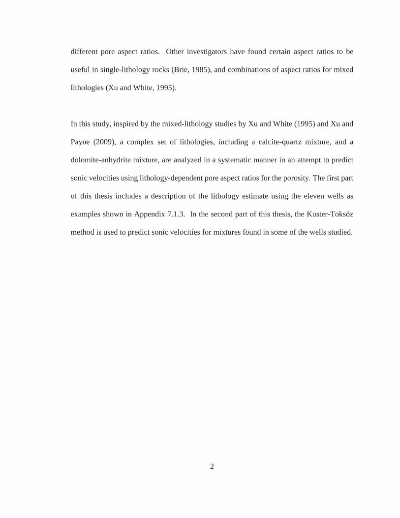
Figure 3.2.5. A log suite for the Kennedy well. Shallower than 2400 ft the lithology is predominantly limestone with quartz, and deeper than 2400 ft it is dolomite with anhydrite.
The first results are represented by the crossplots shown in Figures 3.2.6-8, each using a
depth range depth range of 2100 – 2200 ft. All three of the crossplots clearly illustrate that
this depth section of the well contains limestone with a significant amount of quartz.
14
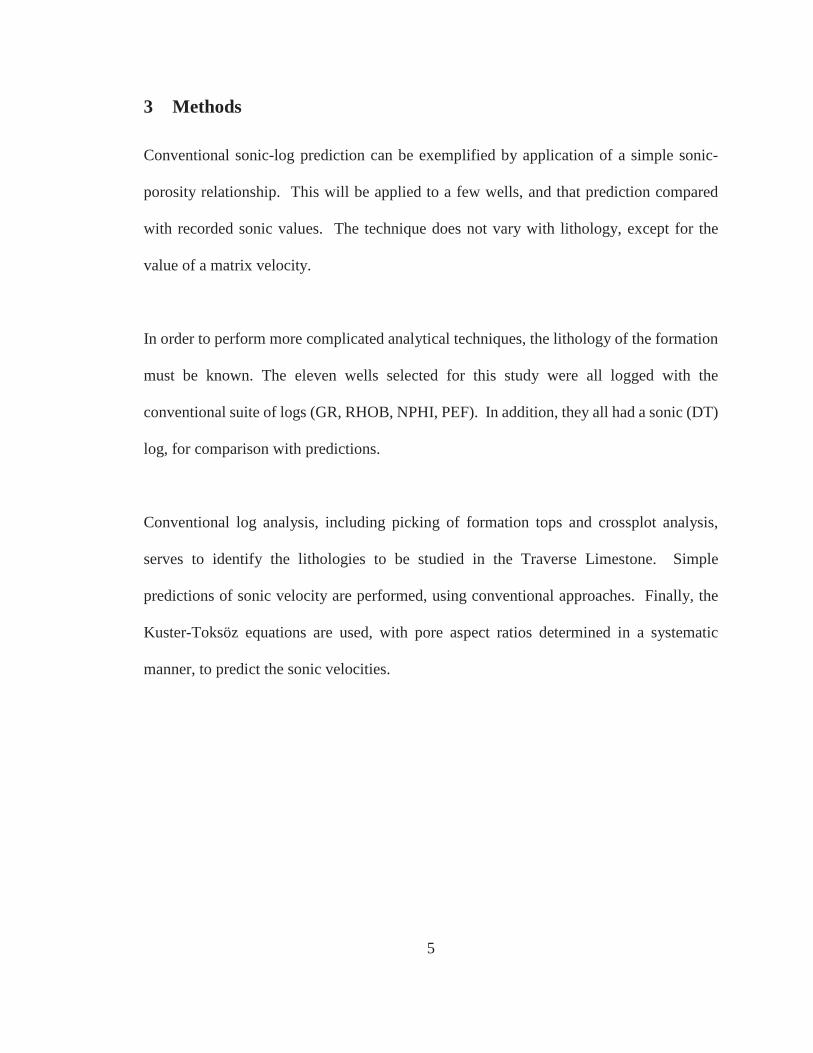
Figure 3.2.6. Density and Neutron porosity crossplot of the Kennedy well, showing limestone and quartz.
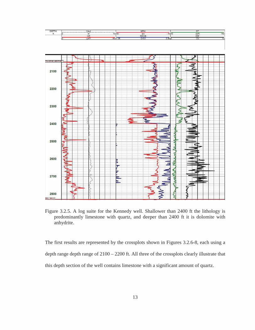
Figure 3.2.7. MID crossplot of UMA and DGA of Kennedy well illustrates the presence of limestone and quartz.
15
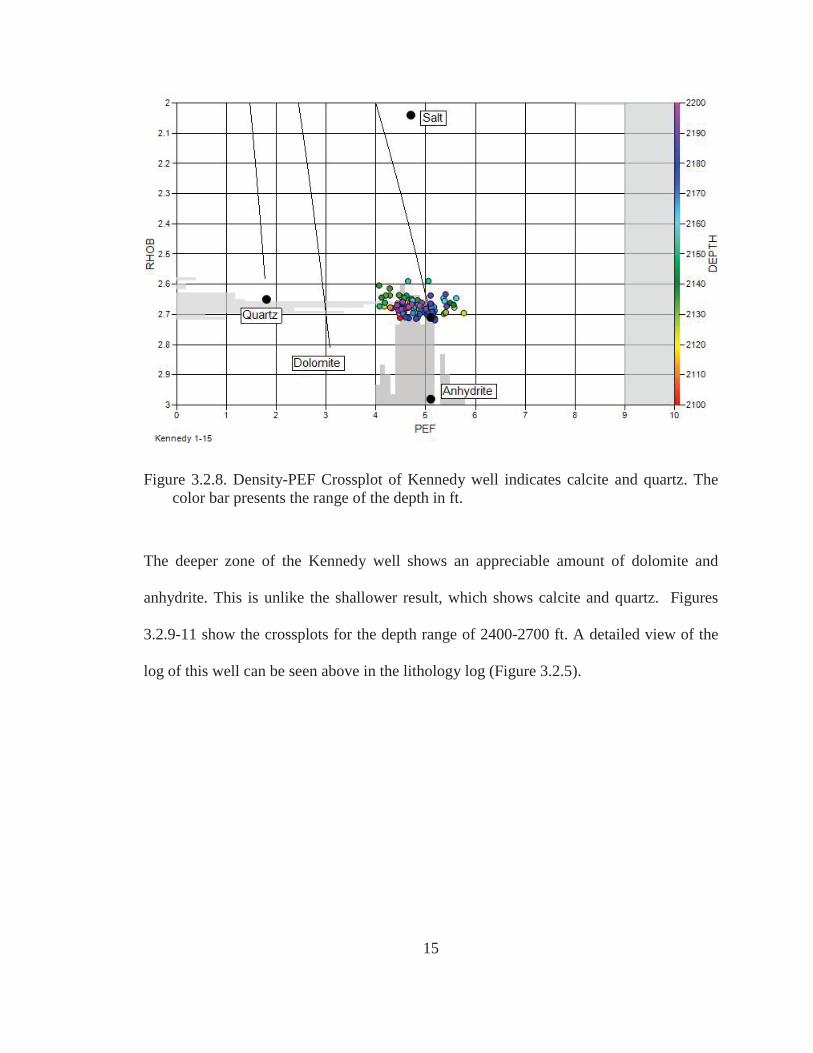
Figure 3.2.8. Density-PEF Crossplot of Kennedy well indicates calcite and quartz. The color bar presents the range of the depth in ft.
The deeper zone of the Kennedy well shows an appreciable amount of dolomite and
anhydrite. This is unlike the shallower result, which shows calcite and quartz. Figures
3.2.9-11 show the crossplots for the depth range of 2400-2700 ft. A detailed view of the
log of this well can be seen above in the lithology log (Figure 3.2.5).

16
Figure 3.2.9. Neutron porosity-Density crossplot of deeper portion of the Kennedy well suggests dolomite and anhydrite, but the interpretation from this plot alone is not unique.
Figure 3.2.10. MID Crossplot of UMA and DGA of Kennedy well indicates dolomite and anhydrite. In this case, the MID plot does not, by itself, indicate the presence of anhydrite, and is non-unique.

17
Figure 3.2.11.Density-PEF Crossplot of Kennedy indicate dolomite and anhydrite. This plot clearly indicates that the mineral combination is dolomite and anhydrite, and together with the other crossplots, the ambiguity is essentially eliminated.

18
3.3 Velocity Determinations
3.3.1 P-wave Velocity Determination from Wyllie’s Time-Average Equation
Wyllie’s Time-Average Equation (Wyllie et al., 1956) is used to estimate the P-wave transit
time using an estimate of porosity. A determination of lithology as described in the
previous section, an estimate of porosity from averaging the porosity logs, and the
assumption of full saturation with slightly brackish water are used to predict the sonic log.
The following form of the equation is used to predict the sonic log;
t = ( tq * Vq + tc * Vc + td * Vd + ta * Va + ts * Vs ) * (1 – ) + tf * (1)
t, tq, tc, td, ta, ts, and tf are, respectively, Travel Times (slownesses) of the bulk
rock and the matrix components quartz, calcite, dolomite, anhydrite, clay and the fluid. Vq,
Vc, Vd, Va and Vs are the fractional volume of the quartz, calcite, dolomite, anhydrite and
clay with respect to the total fractional volume. is total porosity.
The slowness of each mineral is presented in Table 3.3.1 (Pirson, 1983). The fractional
volumes (V) of the minerals were calculated from the crossplots. In the following section,
Figure 3.3.3.2 shows the P-wave velocity obtained from Wyllie’s Time-Average equation.
The predicted P-wave velocity was more accurate in limestone than in layers containing
significant shale or the dolomite zone; where there is shale or dolomite content in the
Traverse formation, the difference between the P-wave velocity observed and the P-wave
velocity from Wyllie’s Time-Average equation increases.
19
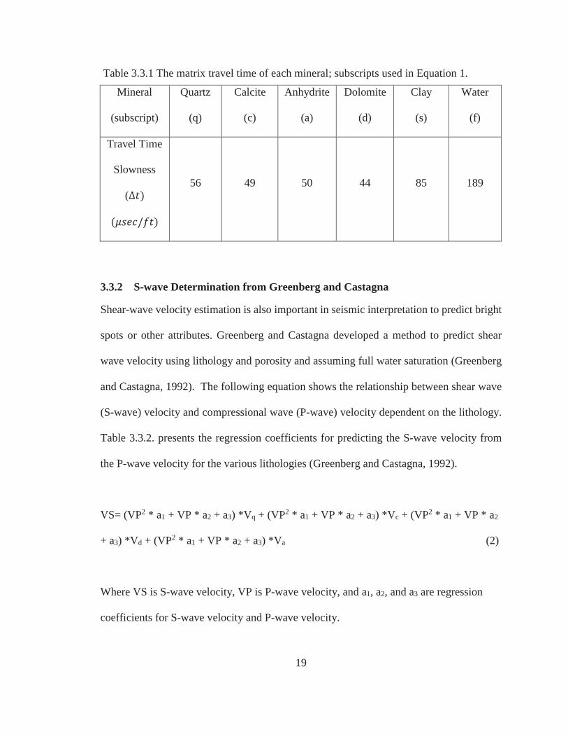
Table 3.3.1 The matrix travel time of each mineral; subscripts used in Equation 1.
Mineral
(subscript)
Quartz
(q)
Calcite
(c)
Anhydrite
(a)
Dolomite
(d)
Clay
(s)
Water
(f)
Travel Time
Slowness
( ) ( / )
56 49 50 44 85 189
3.3.2 S-wave Determination from Greenberg and Castagna
Shear-wave velocity estimation is also important in seismic interpretation to predict bright
spots or other attributes. Greenberg and Castagna developed a method to predict shear
wave velocity using lithology and porosity and assuming full water saturation (Greenberg
and Castagna, 1992). The following equation shows the relationship between shear wave
(S-wave) velocity and compressional wave (P-wave) velocity dependent on the lithology.
Table 3.3.2. presents the regression coefficients for predicting the S-wave velocity from
the P-wave velocity for the various lithologies (Greenberg and Castagna, 1992).
VS= (VP2 * a1 + VP * a2 + a3) *Vq + (VP2 * a1 + VP * a2 + a3) *Vc + (VP2 * a1 + VP * a2
+ a3) *Vd + (VP2 * a1 + VP * a2 + a3) *Va (2)
Where VS is S-wave velocity, VP is P-wave velocity, and a1, a2, and a3 are regression
coefficients for S-wave velocity and P-wave velocity.

20
Table 3.3.2. The regression coefficients (when velocities are in km/s) for P-wave and S-wave velocities in pure porous matrix
Lithology Sandstone Limestone Dolomite Shale
a1 0 -0.05508 0 0
a2 0.80416 1.01677 0.58321 0.76969
a3 -0.85588 -1.03049 -0.07775 -0.86735
Figure 3.3.3.2 shows the results of the S-wave velocity predictions from Greenberg and
Castagna as well as the results of the Kuster-Toksöz model, which will be discussed in the
next section. The relationship between P-wave and S-wave velocities helps to identify
lithology, but in this study, since no S-wave logs were recorded, it is not useful for lithology
identification.
3.3.3 Velocity Determination from Rock Physics Modeling
Predicting sonic velocities in carbonate rocks is complicated. Xu and White (1995)
developed a method of estimating compressional and shear-wave velocities in shaly and
clean sandstone using porosity (Xu and Keys, 2002). The Xu and White (1995) method
depends on the effect of clay content and the pore aspect ratios for the porosities associated
with clays and sands on velocity (Xu and Keys, 2002). The Xu and White (1995) method
estimates dry rock bulk moduli from the Gassmann equation (Gassmann, 1951) and shear
moduli for the mixture of sand by applying the effective medium method of the Kuster-
Toksöz (1974) model (Xu and Keys, 2002). Porosity and pore aspect ratio are the two
major factors in this model. The aspect ratio of a pore depends on the effects of clay,

21
cementation and pressure. Effective pressure affects the closure of the cracks when the
gaps have a low aspect ratio (Xu and Keys, 2002). A relationship between elastic properties
and lithology types was found when testing different aspect ratios of pores in carbonate
rocks for calcite, dolomite, and quartz components.
The Xu-White method relies on the gamma ray responses and porosity determination.
Inspired by the Xu-White method, this study applied a similar approach to the Traverse
Limestone. The Gassmann equation was not applied to find dry-rock values, as the Xu-
White method requires, but instead the method used here simply assumed water-saturated
properties. First, I analyzed rocks that had been determined to contain a mixture of
limestone and quartz. Eventually, more-complex lithologies were considered, including
dolomite and anhydrite. In these examples, I sought the pore aspect ratio that provided
predictions of DT that fit the observed logs best (in an RMS sense). The minimum Root
Mean Square (RMS) error, shown in Appendix 7.2, was found by searching through a
reasonable range of pore aspect ratios and comparing the P-wave velocity predicted with
that which was observed by the DT log. By starting with limestone with quartz, and
gradually adding complexity in the form of other lithologies, I was able, incrementally, to
obtain pore aspect ratios for the additional lithologies.
The mixture properties of bulk modulus and shear modulus were calculated using a
volume-weighted average according to the volume fractions of the components (the Voigt
average for moduli). The bulk modulus and shear modulus of the matrix minerals are given
in Table 3.3.3. (Mavko et all, 2009). The portion of the total porosity assigned to the quartz,
22
calcite, anhydrite, and dolomite components were computed using their volume fractions
(Appendix III), obtained in this study (for simplicity) from crossplots. The total porosity
equals the sum of the porosities of quartz, calcite, anhydrite, and dolomite. The porosity of
the clay fraction is almost zero, which is why the aspect ratio of the clay was not an
important factor. Because of this, the clay in the formation was ignored for the calculations.
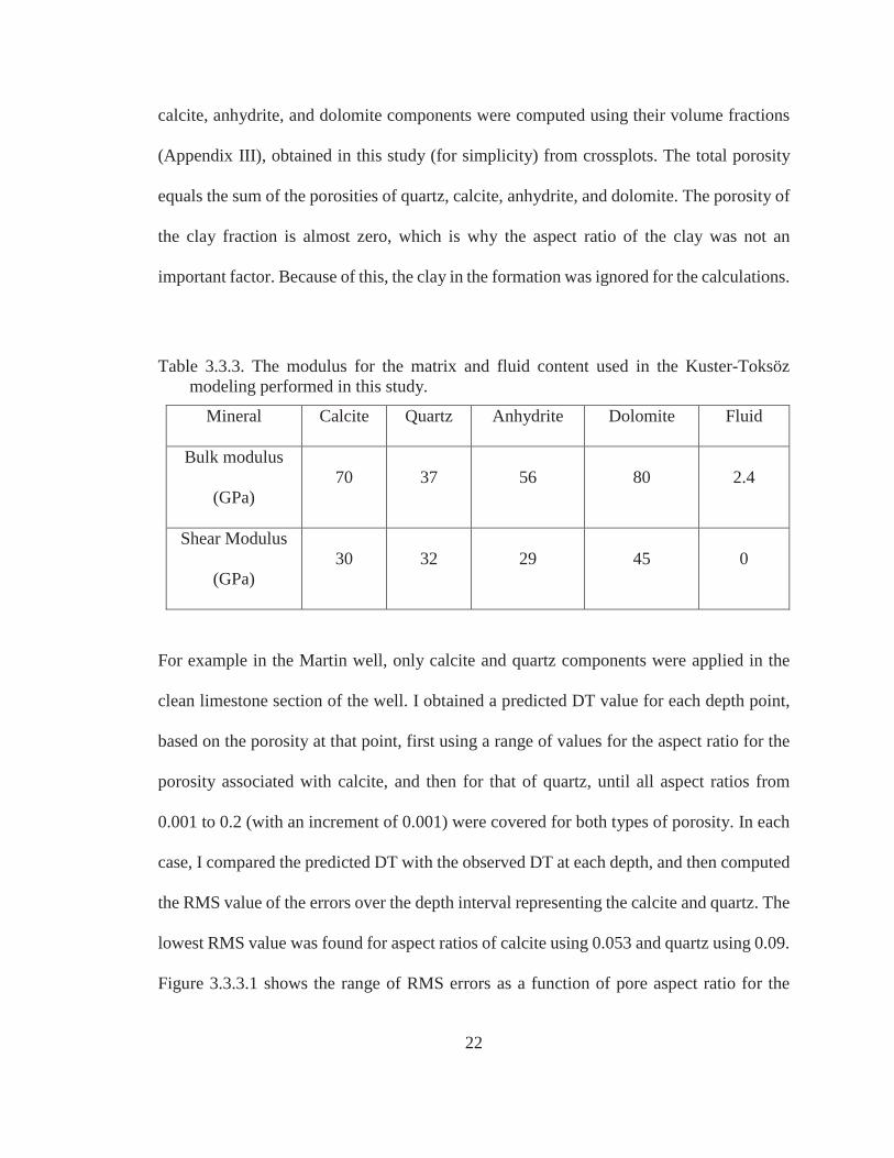
Table 3.3.3. The modulus for the matrix and fluid content used in the Kuster-Toksöz modeling performed in this study.
Mineral Calcite Quartz Anhydrite Dolomite Fluid
Bulk modulus
(GPa) 70 37 56 80 2.4
Shear Modulus
(GPa) 30 32 29 45 0
For example in the Martin well, only calcite and quartz components were applied in the
clean limestone section of the well. I obtained a predicted DT value for each depth point,
based on the porosity at that point, first using a range of values for the aspect ratio for the
porosity associated with calcite, and then for that of quartz, until all aspect ratios from
0.001 to 0.2 (with an increment of 0.001) were covered for both types of porosity. In each
case, I compared the predicted DT with the observed DT at each depth, and then computed
the RMS value of the errors over the depth interval representing the calcite and quartz. The
lowest RMS value was found for aspect ratios of calcite using 0.053 and quartz using 0.09.
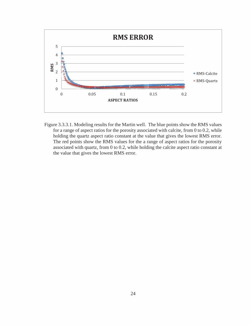
Figure 3.3.3.1 shows the range of RMS errors as a function of pore aspect ratio for the

23
Martin well while holding first one aspect ratio at its best value, then the other aspect ratio
at its best value. We can see in the figure that the aspect ratio of calcite that gives the
smallest RMS error is between 0.04 and 0.06 and the aspect ratio of quartz that gives the
smallest RMS error is between 0.07 and 0.1. However, the RMS error in each case is not
strongly affected by the aspect ratio because the porosity is very small everywhere.
Figure 3.3.3.2. displays the logs for the predicted P-wave velocity (using the technique
described here) and the P-wave velocity computed from the Wyllie Time-Average
Equation for comparison with the observed P-wave velocity from the DT log. It also shows
the S-wave velocity calculated from the approach described here, for comparison with that
obtained by the Greenberg and Castagna approach (recall that no S-wave logs were
available). The P-wave velocity prediction from the Kuster-Toksöz model gives a better fit
to the observed P-wave velocity than that calculated using the Wyllie Time-Average
Equation. The mineral fractions were calculated for the predictions as shown in Appendix
III.
24
Figure 3.3.3.1. Modeling results for the Martin well. The blue points show the RMS valuesfor a range of aspect ratios for the porosity associated with calcite, from 0 to 0.2, while holding the quartz aspect ratio constant at the value that gives the lowest RMS error. The red points show the RMS values for the a range of aspect ratios for the porosity associated with quartz, from 0 to 0.2, while holding the calcite aspect ratio constant at the value that gives the lowest RMS error.
0
1
2
3
4
5
0 0.05 0.1 0.15 0.2
RM
S
ASPECT RATIOS
RMS ERROR
RMS-Calcite
RMS-Quartz

25
Figure 3.3.3.2. The log displays for Traverse Limestone in the Martin well, the P-wave velocity observed (black line), P-wave velocity predicted using Wyllie’s Time Average equation (blue line), and P-wave velocity predicted using Kuster-Toksöz method (red line) in the first track. The second track shows the S-wave velocity (green line) using the Greenberg and Castagna equation and the S-wave velocity predicted (red line) using Kuster-Toksöz method.
26
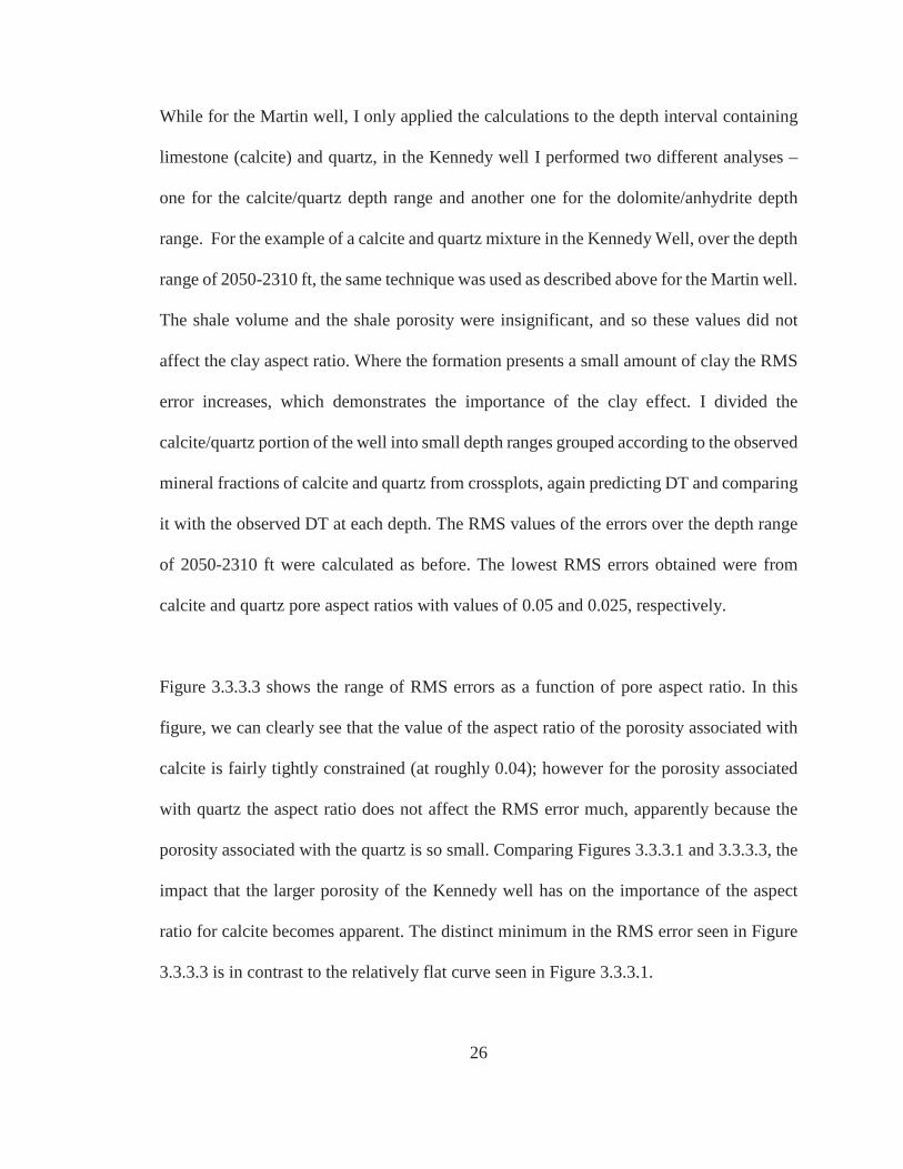
While for the Martin well, I only applied the calculations to the depth interval containing
limestone (calcite) and quartz, in the Kennedy well I performed two different analyses –
one for the calcite/quartz depth range and another one for the dolomite/anhydrite depth
range. For the example of a calcite and quartz mixture in the Kennedy Well, over the depth
range of 2050-2310 ft, the same technique was used as described above for the Martin well.
The shale volume and the shale porosity were insignificant, and so these values did not
affect the clay aspect ratio. Where the formation presents a small amount of clay the RMS
error increases, which demonstrates the importance of the clay effect. I divided the
calcite/quartz portion of the well into small depth ranges grouped according to the observed
mineral fractions of calcite and quartz from crossplots, again predicting DT and comparing
it with the observed DT at each depth. The RMS values of the errors over the depth range
of 2050-2310 ft were calculated as before. The lowest RMS errors obtained were from
calcite and quartz pore aspect ratios with values of 0.05 and 0.025, respectively.
Figure 3.3.3.3 shows the range of RMS errors as a function of pore aspect ratio. In this
figure, we can clearly see that the value of the aspect ratio of the porosity associated with
calcite is fairly tightly constrained (at roughly 0.04); however for the porosity associated
with quartz the aspect ratio does not affect the RMS error much, apparently because the
porosity associated with the quartz is so small. Comparing Figures 3.3.3.1 and 3.3.3.3, the
impact that the larger porosity of the Kennedy well has on the importance of the aspect
ratio for calcite becomes apparent. The distinct minimum in the RMS error seen in Figure
3.3.3.3 is in contrast to the relatively flat curve seen in Figure 3.3.3.1.

27
Figure 3.3.3.3. The scatter plot shows that in the blue line the RMS error changes with therange of calcite’s aspect ratios while holding the quartz’s aspect ratio constant and in the red line the RMS error changes with different range of aspect ratio of quartz while holding the calcite aspect ratio constant at it is best value that gives the lowest RMS error in Kennedy well.
The model for the deeper portion of the Kennedy well uses dolomite and anhydrite
components, over a depth range of 2310-2750 ft. There is assumed to be no porosity
associated with the anhydrite fraction. Still, the dolomite pore aspect ratio does not
significantly affect the RMS error for this depth because there is almost no porosity in the
bulk rock throughout this depth range. Figure 3.3.3.4 displays the RMS errors of the pore
aspect ratio.
00.20.40.60.8
11.21.41.6
0 0.2 0.4 0.6 0.8 1
RM
S
ASPECT RATIO
RMS ERROR
RMS-Calcite
RMS-Quartz

28
Figure 3.3.3.4. This scatter plot shows the RMS error changes with different aspect ratios of dolomite porosity in the Kennedy well with depth range of 2310-2750 ft.
In Figure 3.3.3.5, the observed P-wave velocity was compared with the result that
was obtained using the time-average equation and that predicted using the pore-
aspect ratios found to best fit the compressional wave velocity, all shown in the first
track. In this figure, the second track displays the S-wave velocity obtained from the
Kuster-Toksöz method and that from the Greenberg-Castagna equation. The lithology
log that I interpreted using the mineral fractions was calculated from the MID
crossplot of UMA and DGA and is described in Appendix III with an enlarged example
of the small interval of the depth.
0
2
4
6
8
10
0 0.1 0.2 0.3 0.4 0.5 0.6 0.7 0.8 0.9
RM
S fo
r D
olom
ite
Aspect Ratio
RMS ERROR

29
Figure 3.3.3.5. The log of the Kennedy well with Traverse Limestone where limestone and quartz are present in 2050-2310 ft range and anhydrite and dolomite are present in the 2310-2750 ft depth range (also some between 2090-2260 ft). In the first track, the black line is observed P-wave velocity, the red line displays the predicted P-wave velocity obtained from Kuster-Toksöz and the blue line is P-wave velocity obtained from Wyllie’s Time Equation. In the second track, the red line shows the predicted S-wave velocity obtained from Kuster-Toksöz, and the green line shows the S-wave velocity obtained from Greenberg and Castagna equations. The third track displays the lithology using the method described in the Appendix III.

30
3.4 Pore-type classification There have been other attempts to compare porosities with velocities in an attempt to
determine pore shapes. Here I examine one that uses the measured P-wave velocity and
the total porosity for clean carbonates.
This study used the Xu and Payne (2009) method to classify the pore types, employing
three different pore types similar to the Wang (1991) model (Xu and Payne, 2009). A
carbonate rock displays several different types of pores such as moldic, interparticle, and
microcracks, and these can be related to porosities and velocities.
The elastic properties are assumed to be homogenously distributed throughout the rock.
Typically, moldic pores can be described as round and make the rock stronger than an
equivalent porosity with flatter pores. In addition, the velocity is usually higher when the
pores are interparticle. Microcracks, in contrast, are generally flat and make the rock
weaker with a lower velocity (Xu and Payne, 2009).
Wang et al. (1991), demonstrated the usefulness of a reference line for identifying the effect
of pore types on the P-wave velocity, using laboratory data. This result is used here as two
different reference lines for the dolomite and limestone regions by applying the same
technique to the P-wave velocity of dolomite, which is faster than P-wave velocity of
limestone. The reference line by Wang et al. separates the two regions at the relationship
identified by an aspect ratio of 0.15. The moldic pores are represented by ratios between
0.15-0.8, the aspect ratio of the interparticle pores is assumed to lie directly on the reference

31
line of 0.15, and the aspect ratios of the microcrack pore fall between 0.02-0.15 (Wang et
al., 1991). In the plots, the moldic pores lie above the reference line, the cracks below it,
and the interparticle pores lie directly on the reference line.
From the relationship between porosity and P-wave velocity obtained from Kuster-Toksöz
equation for calcite and quartz in the Kennedy well in figure 3.3.3.6, we can see that almost
all the P-wave velocities are below the reference line, indicating microcrack pores. In
Figure 3.3.3.7 the majority of the relationship between P-wave velocity and porosity is also
in the lower limit of the reference line, which similarly shows microcracks.
Figure 3. The relationship between P-wave velocity estimated from Kuster-Toksöz equation and porosity, showing the pore types of a calcite-quartz mix in the Kennedy well. The black line shows the reference line for limestone which refers to be the aspect ratio of 0.15 demonstrated by Wang et al. (1991)

32
Figure 3. The relationship between P-wave velocity estimated from Kuster-Toksöz equation and porosity, showing the pore types of a dolomite-anhydrite mix in the Kennedy well. The black line shows the reference line for dolomite which refers to be the aspect ratio of 0.15 demonstrated by Wang et al. (1991)

33
4 Results & Discussion
This work attempted petrophysical analysis and rock physics modeling of the Traverse
Limestone formation. Carbonate rocks have a very complex matrix due to different pore
systems, which makes it difficult to predict their velocities. However, examining the
lithology log to identify the minerals in the well help improve velocity prediction using
rock physics modeling.
Mineral identification is achieved by studying the crossplots. The Neutron-density
crossplot and the MID crossplot of UMA and DGA provide indications of the mineral
components; however, the minerals in this system can be identified and seen more clearly
through the PEF-Density crossplot, (especially dolomite and anhydrite). Using all of the
crossplots mentioned above, an accurate result is determined. Identifying mineral
components helps to estimate sonic velocities from different approaches.
Prediction of the P-wave velocity from Wyllie’s Time Average equation was accurate in
clean limestone rocks. In dolomitic formations though, the neutron log gives higher
porosity on a limestone basis than the true porosity. If the porosity is not calculated through
a neutron-density crossplot (or similar calculation), the porosity values obtained are too
high. This gives a large error in the prediction of the P-wave velocity in dolomite using
the typical application of Wyllie’s Time equation. Sonic velocities are predicted from the
Kuster-Toksöz equation and this works well when the mineral identification is accurate.

34
The relationship between the P-wave velocity and porosity also plays an essential role in
the results of this study. We have obtained the best-fit aspect ratios for the calcite
component in the limestone (the other mineral types, including quartz, dolomite, and
anhydrite, have too low a porosity in our examples to provide best-fit aspect ratios). We
have found that the aspect ratio for calcite is about 0.04. Other studies (e.g., Wang et al.,
1991) have compared measured velocities directly with total porosity and classified pore
shapes based on that aspect ratio (0.04). For our data this approach suggests a microcrack
pore type. This determination of the pore types is consistent with the aspect ratios found
from our application of the Kuster-Toksöz method.
35
5 Conclusion
The Traverse Limestone formation is composed of calcite, dolomite, quartz, anhydrite and
a small amount of clay. In addition to the main limestone (calcite) fraction, some parts of
the formation include significant amounts of dolomite, quartz and anhydrite. To determine
these mineral components, the Neutron-density crossplots, MID crossplot of UMA and
DGA crossplots, and the PEF crossplot were used. The mineral fractions determined from
the crossplots were used to calculate the sonic velocities.
Sonic velocities were calculated from different approaches. The P-wave velocity was
predicted using Wyllie’s Time Average equation and the Kuster-Toksöz model. The two
predicted values were then compared with the obtained P-wave velocity. The predicted P-
wave velocity from Kuster-Toksöz model gave the best fit with the observed P-wave
velocity. Furthermore, S-wave velocity was predicted from the Greenberg-Castagna
equation and Kuster-Toksöz model. The predicted S-wave velocities gave similar results
between the two equations, but the observed S-wave velocity was not recorded nor
available for comparison.
The Wang (1991) modeling method was used by those authors to identify three different
pore shapes using the velocities obtained from the Kuster-Toksöz equation. Under a similar
assumption I created my own plot to show the relationship between porosity and the P-
wave velocity obtained from the Kuster-Toksöz method. Combined with the aspect ratios
that I obtained from the Kuster-Toksöz method and the Wang method, the conclusion is

36
that pore shapes generally tend to be microcracks when the formation includes a dolomite-
anhydrite mix and a calcite-quartz mix.

37
6 References
Adcock, S. (1993), In search of the well tie; what if I don’t have a sonic log?, The leading Edge, 12(12), 1161-1164, doi: 10.1190/1.1436929. Brie, A., D. L. Johnson, and R. D. Nurmi (1985), Effect of spherical pores on sonic and resistivity measurements: Presented at SPWLA 26th Annual Logging Symposium. Catacocinos, P. A, W.B. Harrison III, and P.A. Daniels, Jr. (1990), Structure, Stratigraphy, and Petroleum Geology of the Michigan Basin: Chapter 30: Part II. Selected Analog Interior Cratonic Basins: Analog BasinRep., 40 pp. Gassmann, F. (1951), Uber die Elastizität Poröser Medien: Vier. der Natur. Gesellschaft in Zürich 96, 1-23 Greenberg, M. L. and J. P. Castagna (1992), Shear-wave velocity estimation in porous rocks: Theoretical formulation, preliminary verification and applications: Geophysical Prospecting, 40, 195-209 Hasenmueller, N. R., and J. L. Bassett (1979), Maps of northern Indiana showing thicknesses of the Sunbury, Ellsworth, and Antrim Shales (New Albany Shale equivalents): Morgantown, W. Va., U.S. Dept. Energy, Morgantown Energy Technology Center, METC/EGSP Ser. No. 806 [1980]. Hill, R. (1952), The elastic behavior of a crystalline aggregate: Proceedings of the Physical Society, Section A, Volume 65, Issue 5, pp. 349-354 (1952). Huntoon, J. E. and A. S. Wylie Jr. (2003), Log-curve amplitude slicing: Visualization of log data and depositional trends in the Middle Devonian Traverse Group, Michigan basin, United States, AAPG Bulletin, 87(4), 581-608, doi: 10.1306/12040201057. Islam, N. (2011) Sonic log prediction in carbonates, Master's Thesis, Michigan Technological University, 2011. Jordan J. R. and F. L. Campbell (1986) Well Logging II – Electric and Acoustic Logging: SPE Monograph Series, SPE, Dallas, TX Keys, R. G. and S. Xu (2002), An approximation for the Xu-White velocity model, Geophysics, 67, 1406-1414. Kuster, G. T., and M. N. Toksöz (1974), Velocity and attenuation of seismic waves in two-phase media: Part1: Theoretical formulation: Geophysics, Geophysics 39, 587-606.

38
Lilenthal, R.T. (1974), Subsurface Geology of Barry County, Michigan. Geological Survey, 18 pp, Lansing, Michigan. Mavko G, T. Mukerji, and J. Dvorkin (2003), The rock physics handbook: Tools for seismic analysis in porous media. Cambridge University Press, Miller, S. L. M. and R. R. Stewart (1990), Effect of lithology, porosity and shaliness on P- and S-wave velocities from sonic logs: Canadian Journal of Exploration Geophysics, Vol. 26, Nos 1&1, P. 94-103 Prison J. S. (1983), Geologic well log analysis. Gulf Publishing Company, Houston, Texas, 475 pp Pringle, G. H. (1937), Progress Report Number Three, Geology of Arenac County. State of Michigan, 16 pp, Arena County. Sams, M. and T. Focht (2013), An effective inclusion-based rock physics model for a sand-shale sequence: First Break, 31, 61–71 Xu, S. and A. Payne (2009), Modeling elastic properties in carbonate rocks: The Leading Edge, 28, 66-74. Xu, S., and R. E. White (1995), A new velocity model for clay-sand mixtures: Geophysical Prospecting, 43, no. 1, 91–118 Wang Z, W. K. Hirsche and G. Sedgwick (1991), Seicmic velocities in carbonate rock: J. Canadian Petro. Tech., 30, 112-122 Wyllie, M. R. J., Gregory, A. R. & Gardner, G. H. F. 1958. An experimental investigation of factors affecting elastic wave velocities in porous media. Geophysics, 23: 459-93

39
7 Appendices
7.1 Appendix (I): Crossplots
7.1.1 MID of DGA and UMA Crossplot
For this crossplot, apparent grain density and apparent matrix volumetrix cross section with apparent total porosity are required to identify lithology using the data from density and litho-density log. DGA = RHOB RHOB1 PHIND
UMA = PEF RHOB + 0.18831.0704
DGA = Apparent Grain Density
t = Apparent total porosity
UMA = Apparent matrix photo-electric volumetric cross section
PEF = Photoelectric absorption cross section
40
7.1.2 Additional Crossplots of Sampled Wells
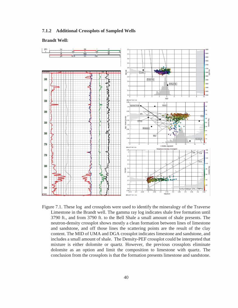
Brandt Well:
Figure 7.1. These log and crossplots were used to identify the mineralogy of the Traverse Limestone in the Brandt well. The gamma ray log indicates shale free formation until 3790 ft., and from 3790 ft. to the Bell Shale a small amount of shale presents. The neutron-density crossplot shows mostly a clean formation between lines of limestone and sandstone, and off those lines the scattering points are the result of the clay content. The MID of UMA and DGA crossplot indicates limestone and sandstone, and includes a small amount of shale. The Density-PEF crossplot could be interpreted that mixture is either dolomite or quartz. However, the previous crossplots eliminate dolomite as an option and limit the composition to limestone with quartz. The conclusion from the crossplots is that the formation presents limestone and sandstone.

41
Figure 7.2. These log and crossplots were used to identify the mineralogy of the Traverse
Limestone in the Coates well. The gamma ray log indicates a shaly formation. The
neutron-density crossplot depicts a clean limestone with shaly formation. The MID of
UMA and DGA crossplot indicates also limestone, and the data points located outside
of the limestone region are the result of the shale content. The Density-PEF crossplot
suggests a composition of calcite and quartz or a composition of calcite and dolomite.
However, the additional crossplot remove the ambiguity of the composition by
narrowing the possibility to quartz. The conclusion from all of the crossplots indicates
that this formation is a shaly limestone.
42
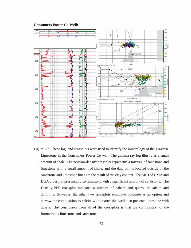
Consumers Power Co Well:
Figure 7.3. These log and crossplots were used to identify the mineralogy of the Traverse
Limestone in the Consumers Power Co well. The gamma ray log illustrates a small
amount of shale. The neutron-density crossplot represents a mixture of sandstone and
limestone with a small amount of shale, and the data points located outside of the
sandstone and limestone lines are the result of the clay content. The MID of UMA and
DGA crossplot presences also limestone with a significant amount of sandstone. The
Density-PEF crossplot indicates a mixture of calcite and quartz or calcite and
dolomite. However, the other two crossplots eliminate dolomite as an option and
narrow the composition to calcite with quartz, this well also presents limestone with
quartz. The conclusion from all of the crossplots is that the composition of the
formation is limestone and sandstone.

43
Gernaat Et Al Well:
Figure 7.4. These log and crossplots were used to identify the mineralogy of Traverse
Limestone at the Gernaat Et Al well. The gamma ray log indicates a small amount of
shale. The neutron-density crossplot indicates shale free limestone, a significant
amount of sandstone and a small amount of dolomite, and the remaining data points
not located within these regions are the result of the clay content . The MID of UMA
and DGA crossplot indicates also the mixture of limestone with a significant amount
of sandstone and small amount of shale free dolomite. The Density-PEF crossplot
shows a mixture of quartz, calcite, and a small amount of dolomite. The final result
from all crossplots is that the Traverse Formation contains limestone, sandstone, and
a small amount of dolomite.

44
Kennedy Well:
Figure 7.5. These log and crossplots were used to identify the mineralogy of the Traverse
Limestone in the Kennedy well. The gamma ray log shows a shale free formation. The
neutron-density crossplot indicates limestone with a significant amount of sandstone
and dolomite. The MID of UMA and DGA crossplot represents a mixture of limestone
with sandstone and dolomite and in the lower region there is a significant amount of
anhydrite. The Density-PEF crossplot presents a mixture of calcite and quartz and a
mixture of dolomite with a significant amount of anhydrite a various location of the
Traverse Limestone. The Density_PEF crossplot indicates that the formation contains
dolomite and anhydrite, underlying limestone and sandstone as depth is indicated in
color.

45
Martin Well:
Figure 7.6. These log and crossplots were used to identify the mineralogy of the Traverse
Limestone in the Martin well. The gamma ray log indicates a small amount of shale,
with a significant amount of shale underlying the formation that indicates a small
amount of shale. The neutron-density crossplot presents free shale formation of
limestone with a significant amount of quartz, and the data points outside of the
limestone and sandstone lines are the result of the clay content. The MID of UMA and
DGA crossplot indicates limestone with sandstone with a significant amount of shale,
and the data points located outside of the limestone and sandstone region as the result
of the clay content as the neutron-density crossplot. The Density-PEF crossplot also
shows a mixture of calcite and quartz. The final result of those crossplots is that the
formation contains limestone with quartz with increasing shaliness in the deeper
section.

46
Prevost Et Al Well:
Figure 7.7. These log and crossplots were used to identify the mineralogy of the Traverse
Limestone in the Prevost Et All well. The gamma ray log indicates a shaly formation.
The neutron-density crossplot presents shale free formation between sandstone and
limestone lines. The MID of UMA and DGA crossplot represents a mixture of
limestone and sandstone and from the ternary diagrams the result of the shale content.
The Density-PEF crossplot also gives a similar result as other two crossplot which
presents calcite and quartz. The conclusion of the all the crossplots is that the
formation contains limestone with significant amount of sandstone.

47
Snowplow Well:
Figure 7.8. These log and crossplots were used to identify the mineralogy of the Traverse
Limestone in the Snowplow well. The gamma ray log indicates a significant amount
shale. The neutron-density crossplot presents clean limestone at a range of the depths
with a small amount of sandstone, and also a significant amount of shale at the various
depths. The MID of UMA and DGA crossplot shows limestone and it also presents a
small amount of sandstone. The Density-PEF crossplot also indicates a mixture of
quartz and calcite. The result of the crossplots is that at various depths the formation
consists of clean limestone, clean limestone with a small amount of sandstone, and
shaly formation.

48
Visser Well:
Figure 7.9. These log and crossplots were used to identify the mineralogy of the Traverse
Limestone in the Visser well. The gamma ray log indicates a small amount of shale.
The neutron-density crossplot presents clean limestone and the data points outside of
the limestone region is the result of a small amount of shale content. The MID of UMA
and DGA crossplot shows also limestone. The Density-PEF crossplot interpretation
present clean calcite. The conclusion of the crossplots is that the formation consists of
clean limestone with small amounts of shale at various depths.

49
Haroutunian Unit Well:
Figure 7.10. These log and crossplots were used to identify the mineralogy of the Traverse
Limestone in the Haroutunian Unit well. The gamma ray log indicates a shaly formation,
and the caliper log gives some error where the formation has shale content. The neutron-
density crossplot presents clean limestone and a small amount of dolomite, while the other
data points the outside of the lines of limestone and dolomite is result of the large shale
content. The MID of UMA and DGA crossplot shows also limestone with a small amount
of dolomite. The Density-PEF crossplot interprets shale free limestone and dolomite, and
scattered data points because of shale, which is demonstrated on the depth axis. The
conclusion of the crossplots is the formation presents clean limestone and dolomite with a
significant amount of shale at the majority of the depth ranges.

50
Huber Well:
Figure 7.11. These log and crossplots were used to identify the mineralogy of the Traverse
Limestone in the Huber well. The gamma ray log indicates a shaly formation. The neutron-
density crossplot presents clean limestone and insignificant dolomite, while the other
scattered data points are out of the limestone region as a result of the large shale content.
The MID of UMA and DGA crossplot shows also limestone with a significant amount of
shale. The Density-PEF crossplot interprets shale free limestone and dolomite, and
scattered data points because of shale, which is depicted on the depth axis. The conclusion
of the crossplots is that the formation presents clean limestone and a very small amount of
dolomite with a significant amount of shale at the majority of the depth ranges.

51
7.2 Appendix (II): Root-Mean-Square (RMS) Error Calculation = (ÿ )
n = Depth
ÿ = Predicted values
y = Observed values
In this study, the depth range is selected to calculate RMS error for over the depth ranges
that are mostly quartz and calcite and that are mostly dolomite and anhydrite.
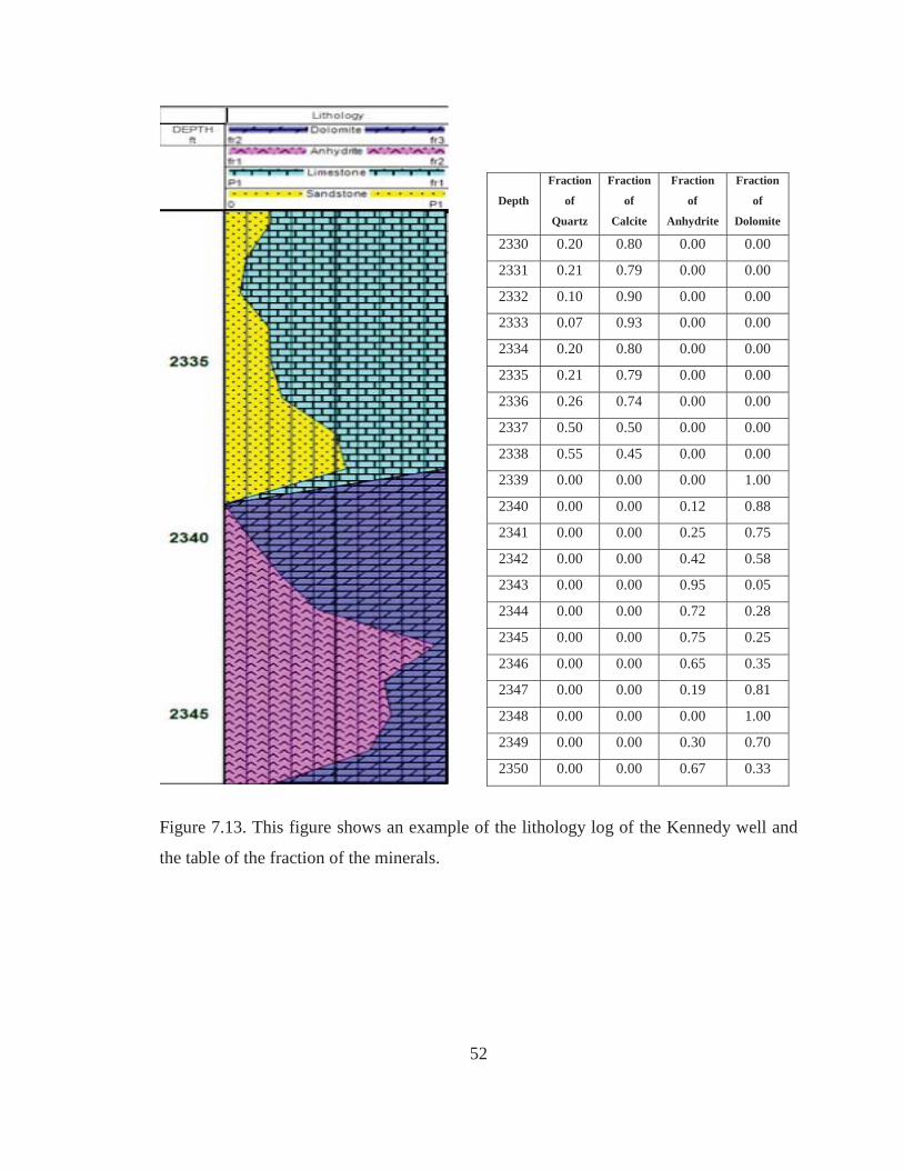
7.3 Appendix (III): Lithology Log The lithology log was made by using the mineral components derived from the crossplots.
The formation includes a small amount of shale which was ignored in the calculations. The
mineral fractional volume of each of the minerals was generally estimated from the ternary
diagram from the MID of DGA and MID crossplot for each depth with cross checking with
the other crossplots. An example of a small depth range of the formation is shown in Figure
7.13, with a table that shows the fractional volume by depth. This example is taken from
the Kennedy well, whose logs and crossplots are shown in Figure 3.2.5-11.
52
Figure 7.13. This figure shows an example of the lithology log of the Kennedy well and
the table of the fraction of the minerals.
Depth
Fraction
of
Quartz
Fraction
of
Calcite
Fraction
of
Anhydrite
Fraction
of
Dolomite
2330 0.20 0.80 0.00 0.00
2331 0.21 0.79 0.00 0.00
2332 0.10 0.90 0.00 0.00
2333 0.07 0.93 0.00 0.00
2334 0.20 0.80 0.00 0.00
2335 0.21 0.79 0.00 0.00
2336 0.26 0.74 0.00 0.00
2337 0.50 0.50 0.00 0.00
2338 0.55 0.45 0.00 0.00
2339 0.00 0.00 0.00 1.00
2340 0.00 0.00 0.12 0.88
2341 0.00 0.00 0.25 0.75
2342 0.00 0.00 0.42 0.58
2343 0.00 0.00 0.95 0.05
2344 0.00 0.00 0.72 0.28
2345 0.00 0.00 0.75 0.25
2346 0.00 0.00 0.65 0.35
2347 0.00 0.00 0.19 0.81
2348 0.00 0.00 0.00 1.00
2349 0.00 0.00 0.30 0.70
2350 0.00 0.00 0.67 0.33

53
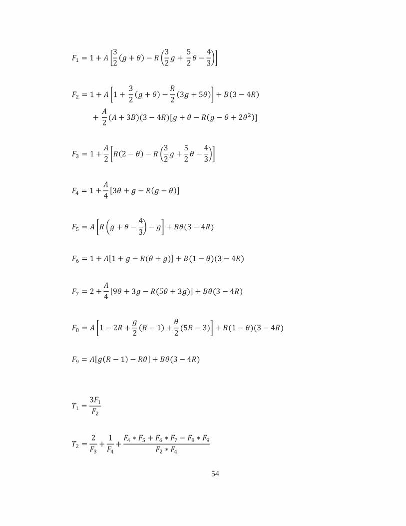
7.4 Appendix (IV): The Kuster-Toksöz Model (1974) The Kuster-Toksöz Model uses a combination of the porosities, the aspect ratios, and the
elastic properties of the different fractions in the matrix to calculate the sonic velocities of
the matrix. For Kuster-Toksöz equation, total porosity was calculated from neutron
porosity log and density log, and the fractions of the minerals were calculated from the
crossplots.
= + = 1
= 1 = The porosity of the matrix = The porosity of the clay
= The volume of the matrix
= The volume of the clay
= (1 ) cos ( ) 1
= 1 (3 2)
= 33 + 4
= 13
= 1
54
= 1 + 32 ( + ) 32 + 52 43
= 1 + 1 + 32 ( + ) 2 (3 + 5 ) + (3 4 ) + 2 ( + 3 )(3 4 )[ + ( + 2 )] = 1 + 2 (2 ) 32 + 52 43
= 1 + 4 [3 + ( )] = + 43 + (3 4 )
= 1 + [1 + ( + )] + (1 )(3 4 )
= 2 + 4 [9 + 3 (5 + 3 )] + (3 4 )
= 1 2 + 2 ( 1) + 2 (5 3) + (1 )(3 4 )
= [ ( 1) ] + (3 4 )
= 3
= 2 + 1 + +
55
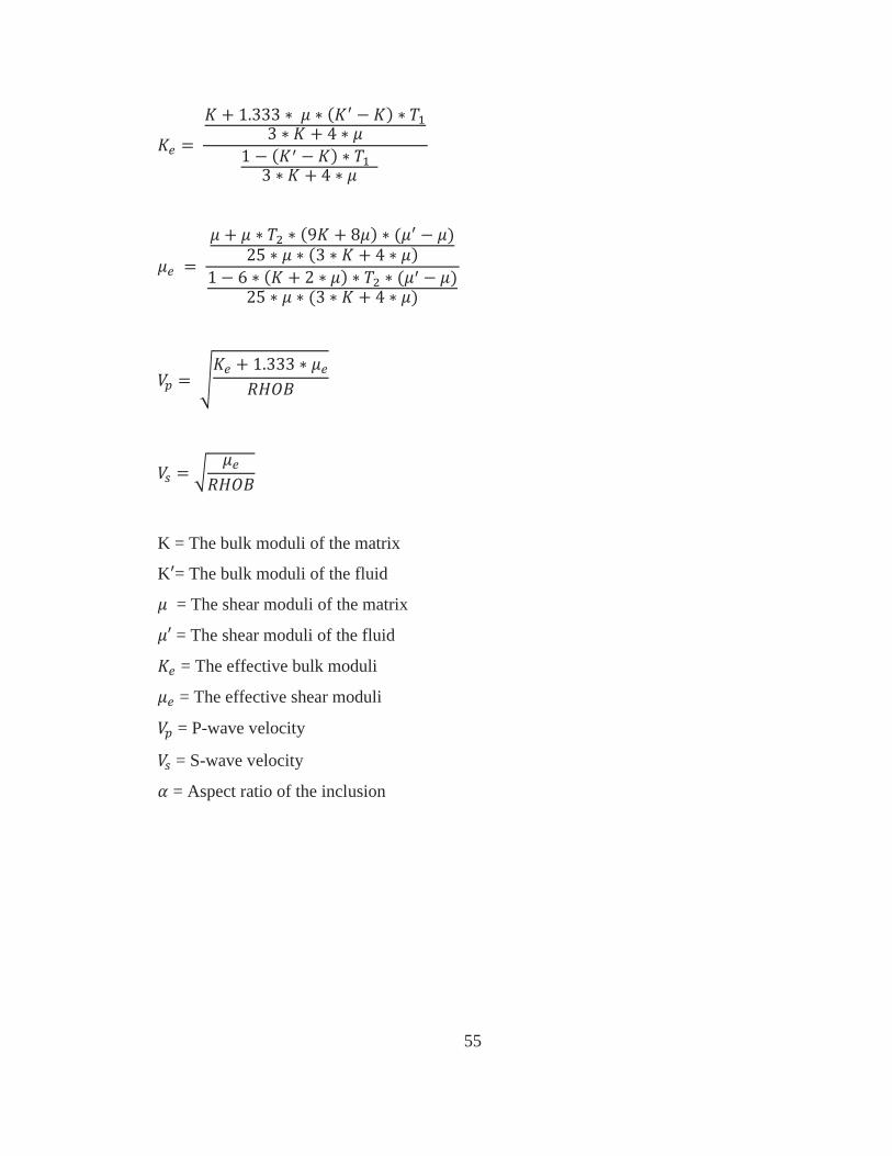
= + 1.333 ( )3 + 41 ( ) 3 + 4
= + (9 + 8 ) ( )25 (3 + 4 )1 6 ( + 2 ) ( )25 (3 + 4 )
= + 1.333
=
K = The bulk moduli of the matrix
K = The bulk moduli of the fluid
= The shear moduli of the matrix
= The shear moduli of the fluid
= The effective bulk moduli
= The effective shear moduli
= P-wave velocity
= S-wave velocity
= Aspect ratio of the inclusion


