Download - Performance Metrics for Estimation Filters

PERFORMANCE METRICS FOR FUNDAMENTAL ESTIMATION FILTERS
A THESIS SUBMITTED TO THE GRADUATE SCHOOL OF NATURAL AND APPLIED SCIENCES
OF MIDDLE EAST TECHNICAL UNIVERSITY
BY
KORAY AKÇAY
IN PARTIAL FULFILLMENT OF THE REQUIREMENTS FOR
THE DEGREE OF MASTER OF SCIENCE IN
ELECTRICAL AND ELECTRONIC ENGINEERING
SEPTEMBER 2005

Approval of the Graduate School of Natural and Applied Sciences
Prof. Dr. Canan ÖZGEN Director
ii
I certify that this thesis satisfies all the requirements as a thesis for the degree of Master of Science.
Prof.Dr. İsmet ERKMEN Head of Department
This is to certify that we have read this thesis and that in our opinion it is fully adequate, in scope and quality, as a thesis for the degree of Master of Science.
Prof. Dr. Mustafa KUZUOĞLU Supervisor Examining Committee Members Prof. Dr. Mübeccel DEMİREKLER (METU,EE)
Prof. Dr. Mustafa KUZUOĞLU (METU,EE)
Prof. Dr. Kemal LEBLEBİCİOĞLU (METU,EE)
Prof. Dr. Gönül Turhan SAYAN (METU,EE)
Elif YAVUZTÜRK (MSc.) (ASELSAN)

iii
I hereby declare that all information in this document has been obtained and presented in accordance with academic rules and ethical conduct. I also declare that, as required by these rules and conduct, I have fully cited and referenced all material and results that are not original to this work. Name, Last Name: Koray AKÇAY Signature :

iv
ABSTRACT
PERFORMANCE METRICS FOR FUNDAMENTAL ESTIMATION FILTERS
Akçay, Koray
M.Sc., Department of Electrical Electrnoics Engineering
Supervisor : Prof. Dr. Mustafa Kuzuoğlu
September 2005, 86 pages
This thesis analyzes fundamental estimation filters – Alpha-Beta Filter, Alpha-Beta-
Gamma Filter, Constant Velocity (CV) Kalman Filter, Constant Acceleration (CA)
Kalman Filter, Extended Kalman Filter, 2-model Interacting Multiple Model (IMM)
Filter and 3-model IMM with respect to their resource requirements and
performance. In resource requirement part, fundamental estimation filters are
compared according to their CPU usage, memory needs and complexity. The best
fundamental estimation filter which needs very low resources is the Alpha-Beta-
Filter. In performance evaluation part of this thesis, performance metrics used are:
Root-Mean-Square Error (RMSE), Average Euclidean Error (AEE), Geometric
Average Error (GAE) and normalized form of these. The normalized form of
performance metrics makes measure of error independent of range and the length of
trajectory. Fundamental estimation filters and performance metrics are implemented
in MATLAB. MONTE CARLO simulation method and 6 different air trajectories
are used for testing. Test results show that performance of fundamental estimation
filters varies according to trajectory and target dynamics used in constructing the
filter. Consequently, filter performance is application-dependent. Therefore, before
choosing an estimation filter, most probable target dynamics, hardware resources
and acceptable error level should be investigated. An estimation filter which
matches these requirements will be ‘the best estimation filter’.
Keywords: Estimation Filters, Error Analysis, Performance Metrics

v
ÖZ
TEMEL KESTİRİM SÜZGEÇLERİ İÇİN PERFORMANS ÖLÇÜTLERİ
Akçay, Koray
Yüksek Lisans, Elektrik-Elektronik Mühendisliği Bölümü
Tez Yöneticisi : Prof. Dr. Mustafa Kuzuoğlu
Eylül 2005, 86 sayfa
Bu çalışma, temel kestirim süzgeçleri: Alpha-Beta, Alpha-Beta-Gamma, Sabit Hız
Kalman, Sabit İvne Kalman, İleri Kalman Süzgeci (EKF), 2-model Etkileşimli
Çoklu Model ve 3-model Etkileşimli Çoklu Model Süzgeçlerini, kaynak
gereksimleri ve performanslarına göre incelemiştir. Kaynak gereksinim kısmında,
kestirim süzgeçleri işlemci kullanım, hafıza ihtiyacı ve karmaşıklıklarına göre
değerlendirilmiştir. En iyi sonucu veren süzgeç Alpha-Beta Süzgeci olmuştur.
Çalışmanın performans inceleme kısmında Etkin Değer (RMS) Hata, Ortalama
Euclidean Hata, Geometrik Ortalama Hata ve bunların normalize edilmiş halleri
kullanılmıştır. Hata hesaplamalarının normalize edilmesi, hataların menzil ve iz
boyundan bağımsız hale gelmesini sağlamaktadır. Kestirim süzgeçlerinin modelleri
ve hata hesaplamaları MATLAB ortamında gerçeklenmiştir. Testler için MONTE
CARLO yöntemi ve 6 farklı hava hedefi izi kullanılmıştır. Test sonuçlarından,
süzgeç performanslarının, temel kestirim süzgeçlerini oluştururken kullanılan hedef
dinamiği ve hedef izlerine göre değiştiği gözlemlenmiştir. Sonuç olarak, süzgeç
performansı uygulamaya bağımlıdır. Böylelikle bir kestirim süzgeci seçmeden önce,
hedeflerin olası hareket dinamikleri, sistemin kaynakları ve kabul edilebilir hata
payları ile ilgili bir çalışmanın yapılması gerekmektedir. Bu ihtiyaçlara cevap
verecek kestirim süzgeci uygulamaya uygun en iyi süzgeç olacaktır.
Anahtar Kelimeler: Kestirim Süzgeçleri, Hata Analizi, Performans Ölçütleri

To My Wife
vi

vii
ACKNOWLEDGMENTS
I would like to thank Prof. Dr. Mustafa Kuzuoğlu for his valuable supervision,
advice and criticism throughout the development and improvement of this thesis.
I would aslo like to express my deepest gratitude to Mr. Ahmet Mumcu for his
understanding and support. I am also grateful to ASELSAN Inc. for facilities
provided for the completition of this thesis.
I would like to extend my special appreciation to my parents for their
encouragement they have given me not only throughout my thesis but also
throughout my life.
Last, but not least I would like to thank my wife for her support. This thesis would
not have been completed without her endless love.

viii
TABLE OF CONTENTS PLAGIARISM...........................................................................................................iii ABSTRACT...............................................................................................................iv ÖZ...............................................................................................................................v ACKNOWLEDGMENTS........................................................................................vii TABLE OF CONTENTS........................................................................................viii LIST OF TABLES.....................................................................................................ix LIST OF FIGURES....................................................................................................x CHAPTER 1 INTRODUCTION................................................................................................... 1 2 ESTIMATION FILTERS........................................................................................ 4
2.1 Estimation .................................................................................................. 4 2.2 Tracking ..................................................................................................... 6 2.3 Filtering ...................................................................................................... 8
2.3.1 Alpha-Beta Filter................................................................................ 8 2.3.2 Alpha-Beta-Gamma Filter................................................................ 10 2.3.3 Kalman Filter ................................................................................... 11 2.3.4 Extended Kalman Filter – EKF........................................................ 17 2.3.5 Interacting Multiple Model Filter – IMM Filter .............................. 21
3 ERROR ANALYSIS............................................................................................. 24 3.1 Root Mean Square Error - RMSE ............................................................ 25 3.2 Average Euclidean Error – AEE.............................................................. 25 3.3 Geometric Average Error – GAE............................................................. 25 3.4 Normalized Error ..................................................................................... 26 3.5 Error Measures for Video Trackers.......................................................... 28
3.5.1 Probability of Detection ................................................................... 29 3.5.2 Degree of Vicinity............................................................................ 30
4 RESOURCE ANALYSIS ..................................................................................... 31 4.1 Memory Requirement .............................................................................. 32 4.2 CPU Usage ............................................................................................... 34 4.3 Algorithm Complexity ............................................................................. 37
5 SIMULATIONS.................................................................................................... 38 5.1 Trajectory Test Data................................................................................. 39
5.1.1 Trajectory – 1 ................................................................................... 39 5.1.2 Trajectory – 2 ................................................................................... 40 5.1.3 Trajectory – 3 ................................................................................... 41 5.1.4 Trajectory – 4 ................................................................................... 42
ix
5.1.5 Trajectory – 5 ................................................................................... 43 5.1.6 Trajectory – 6 ................................................................................... 44
5.2 Simulation Results ................................................................................... 45 5.2.1 Trajectory – 1 ................................................................................... 46 5.2.2 Trajectory – 2 ................................................................................... 52 5.2.3 Trajectory – 3 ................................................................................... 56 5.2.4 Trajectory – 4 ................................................................................... 61 5.2.5 Trajectory – 5 ................................................................................... 65 5.2.6 Trajectory – 6 ................................................................................... 69
5.3 Error vs. Filter Constructers..................................................................... 72 6 CONCLUSION..................................................................................................... 81 7 REFERENCES...................................................................................................... 85

x
LIST OF TABLES TABLES Table 4.1.1 Memory Requirements of Fundamental Estimation Filters…..…….…28

xi
LIST OF FIGURES FIGURES Figure 2.1.1 Founder’s Lifelines of the Probability and Estimation Theory…….5
Figure 2.1.2 Block diagram of State Estimation…………………………………6
Figure 2.2.1 Block diagram of typical Tracking System…………………………8
Figure 2.3.1.1 Block diagram of Alpha-Beta Filter………………………………9
Figure 2.3.2.1 Block diagram of Alpha-Beta-Gamma Filter………………….....11
Figure 2.3.1 Typical Kalman Filter Application………………………………...12
Figure 2.3.1 Summary of Kalman Filter……………………………………… 17
Figure 2.3.4.1 Summary of Extended Kalman Filter……………………………21
Figure 2.3.5.1 Summary of IMM Filter………………………………………….22
Figure 3.1 Estimation Error Vector…………..………………………………….24
Figure 3.4.1 Sensor Measurement Vector……………………………………….26
Figure 3.5.1 Ground Truth and Ground Truth Window…………………………29
Figure 4.1.1 Memory Requirements of Fundamental Estimation Filters………..34
Figure 4.2.1 Making MATLAB a Real-time Application in Windows OS……...35
Figure 4.2.2 CPU Usage of Estimation Filters…………………………………...36
Figure 5.1 Simulation User Interface……………………………………………..38
Figure 5.1.1.1 Trajectory – 1……………………………………………………..40
Figure 5.1.2.1 Trajectory – 2……………………………………………………..41
Figure 5.1.3.1 Trajectory – 3……………………………………………………..42
Figure 5.1.4.1 Trajectory – 4……………………………………………………..43
Figure 5.1.5.1 Trajectory – 5……………………………………………………..44
Figure 5.1.6.1 Trajectory – 6……………………………………………………..45
Figure 5.2.1.1 Simulation Results for Trajectory-1………………………………46
Figure 5.2.1.2 Error Distribution of Alpha-Beta Filter Output…………………...47
Figure 5.2.1.3 Error Distribution of Alpha-Beta-Gamma Filter Output………….48
Figure 5.2.1.4 Error Distribution of CV Kalman Filter Output…………………..48
Figure 5.2.1.5 Error Distribution of CA Kalman Filter Output…………………..49

xii
Figure 5.2.1.6 Error Distribution of EKF Output………………………………...50
Figure 5.2.1.7 Error Distribution of 2-model IMM Filter Output………………..50
Figure 5.2.1.8 Error Distribution of 3-model IMM Output………………………51
Figure 5.2.2.1 Simulation Results for Trajectory-2………………………………52
Figure 5.2.2.2 Error Distribution of Alpha-Beta Filter Output…………………...53
Figure 5.2.2.3 Error Distribution of Alpha-Beta-Gamma Filter Output………….53
Figure 5.2.2.4 Error Distribution of CV Kalman Filter Output…………………..54
Figure 5.2.2.5 Error Distribution of CA Kalman Filter Output…………………..54
Figure 5.2.2.6 Error Distribution for EKF Output………………………………..55
Figure 5.2.2.7 Error Distribution of 2-model IMM Filter Output………………..55
Figure 5.2.2.8 Error Distribution of 3-model IMM Filter Output………………..56
Figure 5.2.3.1 Simulation Results for Trajectory-3………………………………55
Figure 5.2.3.2 Error Distribution of Alpha-Beta Filter Output…………………...57
Figure 5.2.3.3 Error Distribution of Alpha-Beta-Gamma Filter Output………….58
Figure 5.2.3.4 Error Distribution of CV Kalman Filter Output…………………..58
Figure 5.2.3.5 Error Distribution of CA Kalman Filter Output…………………..59
Figure 5.2.3.6 Error Distribution of EKF Output………………………………...59
Figure 5.2.3.7 Error Distribution of 2-model IMM Filter Output………………..60
Figure 5.2.3.8 Error Distribution of 3-model IMM Output………………………61
Figure 5.2.4.1 Simulation Results for Trajectory-4………………………………61
Figure 5.2.4.2 Error Distribution of Alpha-Beta Filter Output…………………...61
Figure 5.2.4.3 Error Distribution of Alpha-Beta-Gamma Filter Output………….62
Figure 5.2.4.4 Error Distribution of CV Kalman Filter Output…………………..62
Figure 5.2.4.5 Error Distribution of CA Kalman Filter Output…………………..63
Figure 5.2.4.6 Error Distribution of EKF Output………………………………...63
Figure 5.2.4.7 Error Distribution of 2-model IMM Filter Output………………..64
Figure 5.2.4.8 Error Distribution of 3-model IMM Filter Output………………..65
Figure 5.2.5.1 Simulation Results for Trajectory-5………………………………65
Figure 5.2.5.2 Error Distribution of Alpha-Beta Filter Output…………………...66
Figure 5.2.5.3 Error Distribution of Alpha-Beta-Gamma Filter Output………….66
Figure 5.2.5.4 Error Distribution of CV Kalman Filter Output…………………..67
Figure 5.2.5.5 Error Distribution of CA Kalman Filter Output…………………..67
Figure 5.2.5.6 Error Distribution of EKF Output………………………………...68
Figure 5.2.5.7 Error Distribution of 2-model IMM Filter Output………………..68
Figure 5.2.5.8 Error Distribution of 3-model IMM Filter Output………………..68
Figure 5.2.6.1 Simulation Results for Trajectory-6………………………………69 xii Figure 5.2.6.2 Error Distribution of Alpha-Beta Filter Output…………………...69
Figure 5.2.6.3 Error Distribution of Alpha-Beta-Gamma Filter Output………….70
Figure 5.2.6.4 Error Distribution of CV Kalman Filter Output…………………..70
Figure 5.2.6.5 Error Distribution of CA Kalman Filter Output…………………..70
Figure 5.2.6.6 Error Distribution of EKF Output………………………………...71
Figure 5.2.6.7 Error Distribution of 2-model IMM Filter Output………………..71
Figure 5.2.6.8 Error Distribution of 3-model IMM Filter Output………………..71
Figure 5.3.1 RMSE vs. CV Kalman Filter Meas. Noise Cov. Matrix Coef……...73
Figure 5.3.2 RMSE vs. CA Kalman Filter Meas. Noise Cov. Matrix Coef……...74
Figure 5.3.3 RMSE vs. EKF Meas. Noise Cov. Matrix Coef…………………….75
Figure 5.3.4 RMSE vs. 2-model IMM Filter Meas. Noise Cov. Matrix Coef……76
Figure 5.3.5 RMSE vs. CV Kalman Filter Proc. Noise Cov. Matrix Coef……….77
Figure 5.3.6 RMSE vs. CA Kalman Filter Proc. Noise Cov. Matrix Coef……….78
Figure 5.3.7 RMSE vs. EKF Proc. Noise Cov. Matrix Coef……………………..79
Figure 5.3.8 RMSE vs. 2-model IMM Filter Proc. Noise Cov. Matrix Coef…….80
xiii
1
CHAPTER 1
INTRODUCTION Predicting future has always been an interesting subject to human being for ages.
While some went after fortune tellers, others tried to figure out the future from past.
Certainly, landing on moon was not achieved by clairvoyants; estimation theory
was ready there to put spacecraft into its orbits with some degree of accuracy. In the
world of estimation theory, one must keep in mind the fundamental assumption that
there is always an estimation error. While dealing with our chaotic cosmos, even
keeping the estimation in a considerable neighborhood of true value is enough.
However, what is the measure of accuracy? Which estimation method is better than
others? What is meant by ‘better’? In this thesis, these questions are tried to be
answered.
Before going further it is essential to give some definitions. One of the most popular
application areas of estimation theory is tracking. Tracking is the estimation of the
state of a moving object (target), based on measurements [1]. To simplify the
tracking problem, there are three basic items: measurement, estimation (filters) and
update. Measurement is acquired via sensors by receiving signals from the
environment. There is always a certain degree of measurement error due to sensors
(system) and environment. Depending on this observation, the next measurement is
estimated. Estimation is the process of inferring the value of a quantity of interest
from indirect, inaccurate and uncertain observations [1]. Next state of the target is
estimated with some degree of accuracy, therefore the whole tracking system
parameters must be updated with the true value of estimation. Updating the whole
tracking system (including estimation filters) makes it ready for the next
measurement with lower estimation error, assuming that the dynamics of the target
remain as it has been estimated. However, in a tracking system the dynamics of a

2
target can only be a model of the real life, as it is in all engineering areas. Therefore,
we must be assured that there is always an estimation error to be taken into account.
Estimation Error is the deviation from the estimatee value of the estimated
quantity. Estimatee is the quantity to be estimated. There are several methods for
error analysis. The aim of this thesis is to define an error term more meaningful and
useful to compare and evaluate estimation filters (or systems with estimation
filters).
In the second chapter, a brief background knowledge about Estimation, Tracking,
and Filtering is given. In Filtering sub-section, fundamental estimation filters (in
simple-to-complex order)
• Alpha-Beta Filter,
• Alpha-Beta-Gamma Filter
• Kalman Filter
• Extended Kalman Filter
• Interacting Multiple Model Filter
are discussed.
In the third chapter, error analysis of estimation filters is discussed. The following
Error measure methods are covered
• Root-mean-square Error
• Average Euclidean Error
• Geometric Average Error
• Normalized Error
Besides, Error Measures for Video Trackers is discussed.
In the fourth chapter, Resource Analysis of Filters: Memory Usage, CPU Usage,
and Complexity of Filters are investigated. When implementing an estimation filter
in an embedded hardware one must consider the requirements of filter despite of
limited resources of hardware.

3
In the fifth chapter, the results of simulations are discussed. Test trajectories used in
simulations and Error vs. Filter Constructers are demonstrated here.
In the sixth chapter, suggestions and conclusions on filters and error analysis are
given.

4
CHAPTER 2
ESTIMATION FILTERS
2.1 Estimation ‘Estimation is the process of inferring the value of a quantity of interest from
indirect, inaccurate and uncertain observations’ [1].
As a mathematical concept, the inevitability of measurement errors had been
recognized since the time of Galileo Galilei (1564-1642). The first method dealing
with these errors and forming an optimal estimate from noisy data is the method of
least squares by Carl Freidrich Gauss (1777-1855).
One of the greatest discoveries in the history of statistical estimation theory is
Kalman Filtering by Rudolf Emil Kalman (1930 - …). It has great value of
controlling complex dynamic systems such as aircraft, ships, or spacecraft. For
these applications, it is not always possible to measure every variable that you want
to control. Kalman Filter provides a means of inferring the missing information
from noisy measurements. In the following chapters, details of Kalman Filtering
will be given.
The fundamentals of Kalman Filtering depends on The Theory of Probability, so it
is worth to give brief historical milestones in this branch of mathematics. The
Italian Giroloma Cardano (1501-1576) stated that the accuracies of empirical
statistics tend to improve with the number of trials. Then, general treatments of
probabilities were followed by Blaise Pascal (1623-1662), Pierre De Fermat
(1601-1655), and Christian Huygens (1629-1695). James Bernoulli (1654-1705)
(considered to be the founder of probability by some historians) gave the first
rigorous proof of the law of large numbers. Thomas Bayes (1702-1761) derived the
famous rule for statistical inference. Abraham de Moivre (1667-1754), Pierre Simon

Marquis de Laplace (1749-1827), Adrien Marie Legendre (1752-1833), and Carl
Freidrich Gauss (1777-1855) continued development into the nineteenth century. In
the nineteenth and twentieth century, the probabilities began to take on more
meaning as physically significant attributes. James Clerk Maxwell (1831-1879)
established the probabilistic treatment of natural phenomena as a scientific
discipline. Andrei Nikolaevoich Kolmogorov (1903-1987) and H. Ya Khinchin
worked on the theory of random processes and the foundations of probability theory
on measurement theory. Norbert Wiener (1894-1964) was the first working on the
theory of optimal estimation for systems involving random processes. [2] The
lifelines of important names in the history of probability theory are shown in
Figure-2.1.1
1500 1600 1700 1800 1900 2000
CardanoGalileo
FermatPascal
HuygensNewton
BernoulliBayes
Laplace
LegendreGauss
MaxwellMarkovCholesky
WienerKolmogorov
KalmanBierman
1500 1600 1700 1800 1900 2000
CardanoGalileo
FermatPascal
HuygensNewton
BernoulliBayes
Laplace
LegendreGauss
MaxwellMarkovCholesky
WienerKolmogorov
KalmanBierman
Figure-2.1.1 Founder’s Lifelines of the Probability and Estimation Theory [2]
When talking about estimation, one of the confusing topics is decision. Decision is
the selection of one (the best choice) of a set of discrete alternatives [1]. Estimation
is interpreted as the possibility of not making a choice but obtaining some
conditional probabilities of the various alternatives.
5
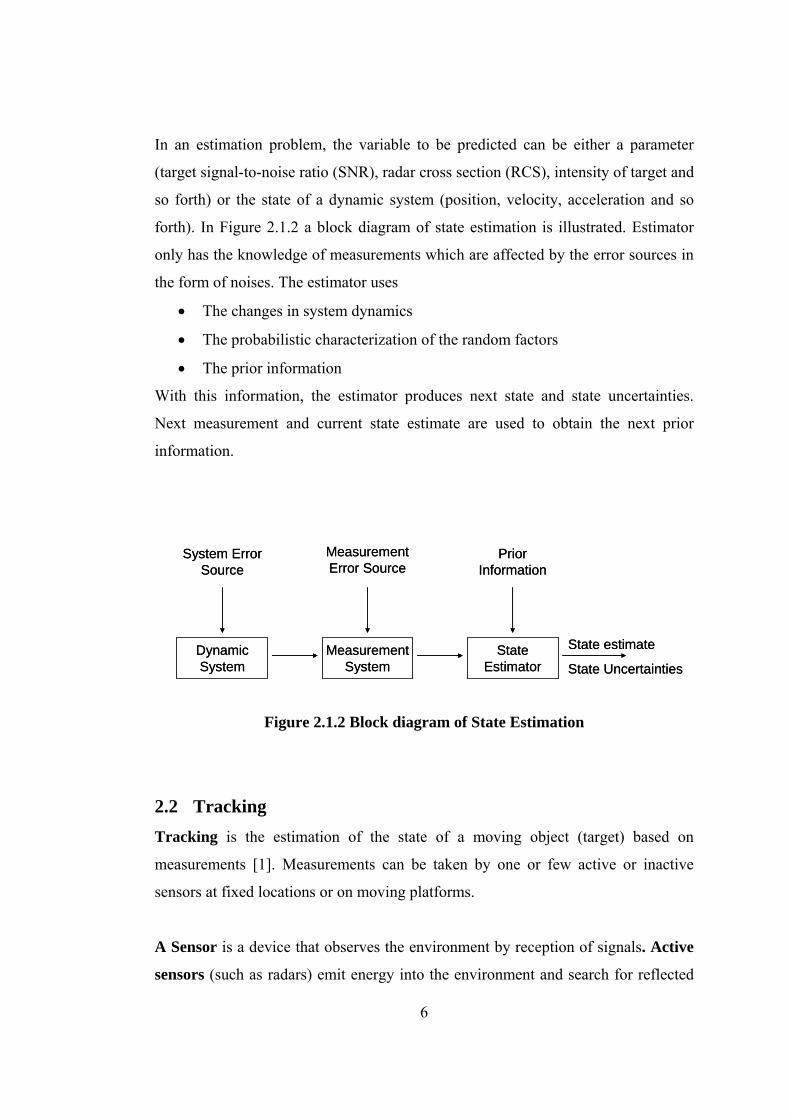
In an estimation problem, the variable to be predicted can be either a parameter
(target signal-to-noise ratio (SNR), radar cross section (RCS), intensity of target and
so forth) or the state of a dynamic system (position, velocity, acceleration and so
forth). In Figure 2.1.2 a block diagram of state estimation is illustrated. Estimator
only has the knowledge of measurements which are affected by the error sources in
the form of noises. The estimator uses
• The changes in system dynamics
• The probabilistic characterization of the random factors
• The prior information
With this information, the estimator produces next state and state uncertainties.
Next measurement and current state estimate are used to obtain the next prior
information.
DynamicSystem
MeasurementSystem
StateEstimator
System Error Source
Measurement Error Source
Prior Information
State estimate
State UncertaintiesDynamicSystem
MeasurementSystem
StateEstimator
System Error Source
Measurement Error Source
Prior Information
State estimate
State Uncertainties
Figure 2.1.2 Block diagram of State Estimation
2.2 Tracking Tracking is the estimation of the state of a moving object (target) based on
measurements [1]. Measurements can be taken by one or few active or inactive
sensors at fixed locations or on moving platforms.
A Sensor is a device that observes the environment by reception of signals. Active
sensors (such as radars) emit energy into the environment and search for reflected
6

7
energy, while passive sensors (such as cameras) search for energy emitted from the
target(s) [3].
Sensors at fixed locations deal only with the dynamics of the target, while sensors
on moving platforms has to take the dynamics of the moving platform into account
which makes the tracking problem more complex.
Tracking is an element of a wider system that performs surveillance, guidance,
obstacle avoidance, etc. Besides using all tools from estimation, tracking requires
extensive use of statistical decision theory. In Figure 2.2.1 a block diagram of a
typical tracking system is illustrated.
A typical multi target tracking system has the following common blocks [4]:
• Tracking Filters: The role of a tracking filter is to carry out recursive target
state estimation. The most common tracking filters are the fixed coefficient
filters (alpha-beta, alpha-beta-gamma), the Kalman Filter and the Extended
Kalman Filter (EKF). In the next section, details of these filters are given.
• Maneuver handling logic: Target motion can change suddenly, and the
tracker must adapt itself to changes in dynamics of target motion. Dynamic
models can be stationary, constant velocity, constant acceleration, etc.
Tracking system has to recognize changes and must choose the most
suitable dynamic model among others.
• Gating and data association: In a multi target environment, the tracking
system has to decide which measurement belongs to which track in order to
identify the origin of measurement.
• Track life management: Track status is typically defined in terms of three
life stages: tentative, confirmed and deleted track. By a tentative target it is
meant that a track has been initiated but not associated with any existing
track. In a confirmed track, measurements are consistent and associated with
an existing track. If for a certain time no track update is performed, than the
track is deleted.

Sensor Signal Processing
DataProcessing
Target State Estimates
Estimate uncertainities
Noise
Environment Sensor Sensor Tracking
Sign
al
Mea
sure
men
t
Sensor Signal Processing
DataProcessing
Target State Estimates
Estimate uncertainities
Noise
Environment Sensor Sensor Tracking
Sign
al
Mea
sure
men
t
Figure 2.2.1 Block diagram of typical Tracking System
2.3 Filtering Commonly, a filter is a physical device for removing unwanted fractions of
mixtures. In electronics the term “filter” was first applied to analog circuits that
filter (attenuate unwanted frequencies) electronic signals. In Estimation Theory,
filtering is the estimation of the current state of dynamic system. Here, the phrase
‘filtering’ is used for obtaining the ‘best estimate’ from noisy data which amounts
to ‘filtering out’ the noise.
Below, five fundamental filters in practical tracking problems (Alpha-Beta Filter,
Alpha-Beta-Gamma Filter, Kalman Filter, Extended Kalman Filter, and Interacting
Multiple Model – IMM Filtering) are discussed in historical - also simple to
advanced - order.
2.3.1 Alpha-Beta Filter
The Alpha-Beta Filter is the simplest constant-gain tracking algorithm. The tracker
has poor performance, but requires a very low computational load. The Alpha-Beta 8

Filter is used in tracking systems where position measurement updates are available
and the state vector consists of positions and velocities. The value of the gain is
preset for handling straight-line motion or turning motion. When the gain is set to
compensate for turning motion in a target, the straight-line performance will suffer
somewhat which is the trade-off for most filters below.
The structure of the Alpha-Beta Filter is based on the error estimation of a position
vector measurement. For example, if we suppose that the velocity of the X variable
is constant, we can predict (prediction phase) the position at time sample k+ 1.
)(*)()1( kVTkXkX p +=+ (2.3.1.1)
However, if the target maneuverability is not null we can update (update phase) this
prediction by adding a percentage of the error.
[ ])1()1()1()1( +−+++=+ kXkzAlphakXkX pp (2.3.1.2)
where, )1( +kz is the position measurement and Alpha is the first tracking
parameter. The same principle is used to attenuate the velocity noise. This new
updated velocity will be used for next prediction.
[ ])1()1()/()()1( +−++=+ kXkzTBetakVkV p (2.3.1.3)
+ +
Z-1
Filtered Position
+
+Filtered Velocity
Z-1
Predicted Position
Position
Alpha
Beta/T T
+ +
Z-1
Filtered Position
+
+Filtered Velocity
Z-1
Predicted Position
Position
Alpha
Beta/T T
Figure 2.3.1.1 Block diagram of Alpha-Beta Filter
9

2.3.2 Alpha-Beta-Gamma Filter
Alpha-Beta-Gamma Filter is similar to Alpha-Beta Filter but acceleration is
included into the state vector besides position and velocity. Only a few summations
and multiplications are added, so it also requires a very low computational load
similar to the Alpha-Beta Filter. Still only position update is needed.
As in the Alpha-Beta Filter, the structure of Alpha-Beta-Gamma Filter is based on
the error estimation of a position vector measurement. Suppose that the acceleration
of the X variable is constant, we can predict (prediction phase) the position at time
sample . 1+k
2/))(*()(*)()1( 2 kATkVTkXkX p ++=+ (2.3.2.1)
However, if there is a maneuver, we can update (update phase) this prediction by
adding a percentage of the error.
[ ])1()1()1()1( +−+++=+ kXkzAlphakXkX pp (2.3.2.2)
where, is the position measurement. The same principle is used for the
velocity and acceleration noise, these new values are used for the next prediction.
)1( +kz
[ ])1()1()/()()1( +−++=+ kXkzTBetakVkV p (2.3.2.3)
[ ]))1()1((*)/)*2(()()1( 2 +−++=+ kXkzTGammakAkA p (2.3.2.4)
10

+ +
Z-1
Filtered Position
+
+Filtered Velocity
Z-1
Predicted Position
Position
+
Z-1
Filtered Acceleration
Alpha
Beta/T
(2*Gamma)/T^2
T
(T^2)/2
+ +
Z-1
Filtered Position
+
+Filtered Velocity
Z-1
Predicted Position
Position
+
Z-1
Filtered Acceleration
Alpha
Beta/T
(2*Gamma)/T^2
T
(T^2)/2
Figure 2.3.2.1 Block diagram of Alpha-Beta-Gamma Filter
2.3.3 Kalman Filter
R.E. Kalman published his paper on recursive solution to the discrete-data linear
filtering in 1960, which is relatively recent although its root is as far back as C.F.
Gauss (1777-1855). Since that time, Kalman Filter has been applied in many
diverse areas like military, aerospace, nuclear plant, economics (even it is not
successful in economics) etc.
The Kalman filter is a multiple-input, multiple-output digital filter that can
optimally estimate, in real time, the states of a system based on its noisy outputs [7].
Here optimal means an algorithm that minimizes chosen error criteria. Since the
filter is recursive, it does not require all previous data to be kept in storage. This
makes it easier to implement Kalman Filter by hardware. The Kalman Filter
11

supports estimations of past, present and future states even when the precise nature
of the modeled system is unknown.
The fundamental assumption about the Kalman Filter is that the state is evaluated
with a known linear system equation which means that the filter is not designed to
handle maneuvering targets.
System
Sensors
System error
Measurement error
Controls
Observed Meas. KalmanFilter
Optimal estimate of system state
System
Sensors
System error
Measurement error
Controls
Observed Meas. KalmanFilter
Optimal estimate of system state
Figure 2.3.1 Typical Kalman Filter Application [9]
In dynamic systems, the state equations are expressed in matrix form. For example,
1+nX = (2.3.3.1) nXH ×
where
⎥⎦
⎤⎢⎣
⎡=
n
nn x
xX
& (2.3.3.2)
and
H = (2.3.3.3) ⎥⎦
⎤⎢⎣
⎡1 T
01
represents state transition matrix for the constant velocity target.
It is now simpler to give the random system dynamics model. Specifically, it
becomes
12

nnn UXHX +×=+1 (2.3.3.4)
where
⎥⎦
⎤⎢⎣
⎡=
nn u
U0
(2.3.3.5)
is the dynamic model noise vector.
We now express the trivial measurement equation in matrix form. It is given by
nnn NXFY +×= (2.3.3.6)
where
][[ ][ ] matrixt measuremen
errorn observatio matrixn observatio 0 1
nn
nn
yYvN
F
===
(2.3.3.7)
Equation 2.3.3.6 is called the observation system equation. This is because it relates
the quantities being estimated to the parameter being observed, which are not
necessarily to be the same. The parameters and (target range and velocity) are
being estimated (tracked) while only target range is observed. As another example,
one could track a target in rectangular coordinates (x,y,z) and make measurements
on the target in spherical coordinates (R,
nx nx&
θ ,φ ). In this case the observation matrix
F would transform from the rectangular coordinates being used by the tracking
filter to the spherical coordinates in which the radar makes its measurements.
nnnn XHX ,,1~~ ×=+ (2.3.3.8)
where
⎥⎥⎦
⎤
⎢⎢⎣
⎡=
nn
nn
nn x
xX
,
,
, ~
~~
& (2.3.3.9)
⎥⎥⎦
⎤
⎢⎢⎣
⎡=
+
+
+nn
nn
nn x
xX
,1
,1
,1 ~
~~
& (2.3.3.10)
13

This is called the prediction equation, because it predicts the position and velocity
of the target at time n+1 based on the position and velocity of the target at time n,
the predicted position and velocity being given by the state vector. Putting into
matrix form yields
)~ - ( ~~1,1,, −− ××+= nnnnnnnn XFYKXX (2.3.3.11)
This is called the Kalman Filtering equation because it provides the updated
estimate of the present position and velocity of the target. Since only position and
velocity are involved, this called Constant Velocity Kalman Filter. If acceleration
is added to the dynamic model, then the filter will be a Constant Acceleration
Kalman Filter. In Constant Velocity model, the response of the filter is faster then
Constant Acceleration model. However, although the response of the constant
velocity filter is faster, the rate of overshooting in the changes is much more than
the Acceleration model. In this work, both Constant Velocity and Constant
Acceleration Kalman Filters are implemented.
The matrix is a matrix giving the tracking-filter constants It is
given by
nK . and nn hg
⎥⎥⎥
⎦
⎤
⎢⎢⎢
⎣
⎡=
Thg
K n
n
n for the two-state alpha-beta or Kalman filter equations. This
form does not however tell us how to obtain In Kalman filter
application is obtained from
. and nn hg
nK
[ ] 11,1,
~ ~ −−− ××+××= T
nnnT
nnn FPFRFPK (2.3.3.12)
where predictor equation
~~1,1, n
Tnnnn QHPHP +××= −− (2.3.3.13)
and dynamic model noise covariance
[ ] [ ] Tnnnn UUEUCOVQ == (2.3.3.14)
[ ]1,1,1,1,~~)~(~
−−−− == nnT
nnnnnn XXEXCOVP (2.3.3.15)
(2.3.3.16) )()( Tnnnn NNENCOVR ==
14

[ ] )~(~2,11,11,1 −−−−−− ××−== nnnnnnn PFKIXCOVP (2.3.3.17)
Covariances apply as long as the entries of the column matrices
zero mean. Otherwise they have to be replaced by
nn NU and have
[ ] [ ]nnnn NENUEU −− and ,
respectively.
Physically, the matrix nnP ,1~
− is an estimate of our accuracy in predicting the target
position and velocity at time n based on the measurements made at time n-1. Here,
1,~
−nnP is the covariance matrix of the state vector 1,~
−nnX . To get a better feeling for
nnP ,1~
− , let us write it out for our two-state 1,~
−nnX .
)~~()~(1,1,1,
Tnnnnnn XXEXCOV−−− = = E ( ][ 1,1,
1,
1, ~ ~~
~−−
−
−
⎥⎥⎦
⎤
⎢⎢⎣
⎡nnnn
nn
nnxx
x
x&
)
= ⎥⎥⎦
⎤
⎢⎢⎣
⎡
−
−−
−−
−
)~(
)~~(
)~~(
)~(2
1,
1,1,
1,1,
21,
nn
nnnn
nnnn
nn
xE
xxE
xxE
xE&
&
&
= 1,~
−nnP (2.3.3.18)
[ ][ ][ ]2
v
2 )(
)(
σ=
=
==
n
Tnnnn
vE
vvENCOVR
(2.3.3.19)
The matrix gives the accuracy of the radar measurements. It is the covariance
matrix of the measurement error vector . For two-state filter, where it is assumed
that
nR
nN
xv σσ and are the root-mean-square of and , the assumption is that the
mean of is zero.
nv nx
nv
15
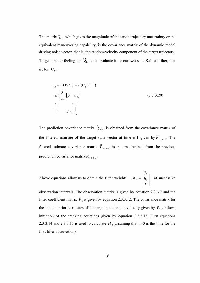
The matrix , which gives the magnitude of the target trajectory uncertainty or the
equivalent maneuvering capability, is the covariance matrix of the dynamic model
driving noise vector, that is, the random-velocity component of the target trajectory.
To get a better feeling for , let us evaluate it for our two-state Kalman filter, that
is, for .
nQ
nQ
nU
][
⎥⎦
⎤⎢⎣
⎡=
⎥⎦
⎤⎢⎣
⎡=
==
)(
0
00
) 00
(
)(
2n
nn
Tnnnn
uE
uu
E
UUECOVUQ
(2.3.3.20)
The prediction covariance matrix 1,~
−nnP is obtained from the covariance matrix of
the filtered estimate of the target state vector at time n-1 given by 1,1~
−− nnP . The
filtered estimate covariance matrix 1,1~
−− nnP is in turn obtained from the previous
prediction covariance matrix 2,1~
−− nnP .
Above equations allow us to obtain the filter weights
⎥⎥⎥
⎦
⎤
⎢⎢⎢
⎣
⎡=
Thg
K n
n
n at successive
observation intervals. The observation matrix is given by equation 2.3.3.7 and the
filter coefficient matrix is given by equation 2.3.3.12. The covariance matrix for
the initial a priori estimates of the target position and velocity given by allows
initiation of the tracking equations given by equation 2.3.3.13. First equations
2.3.3.14 and 2.3.3.15 is used to calculate (assuming that n=0 is the time for the
first filter observation).
nK
1,0 −P
0H
16

In Kalman Filtering, we can simply think that there are two stages: Time Update
and Measurement Update. In Time Update, prediction of the next observation is
calculated. In Measurement Update, the items of Time Update are corrected. In
literature Time Update is called Predictor and Measurement Update is called as
Corrector. Below is the summary of Kalman Filtering in two stage form.
Figure 2.3.1 Summary of Kalman Filter [6]
2.3.4 Extended Kalman Filter – EKF The fundamental assumption about the Kalman Filter is that it is based on linear
system equations where it expects linear measurements. This assumption makes
Kalman Filter weaker for observations from non-linear target dynamics. In most
cases due to the nature of sensors and target dynamics, the measurements are non-
linear. Extended Kalman Filter (EKF) solves this problem. The aim of EKF is to
estimate the state under the conditions of non-linear measurement processes and/or
non-linear target dynamics. The extended Kalman filter (EKF) is a Kalman filter
that linearizes the dynamic system about the current mean and covariance.
17

The nonlinear transformation may introduce bias to the solution, the covariance
calculation is not necessarily accurate, and the EKF can diverge if the initial
conditions are inaccurate. So it is crucial to use a coherent filter or take first few
measurements to initialize the EKF.
Linearization of the estimation around the current estimate using the partial
derivatives of the process is just like a Taylor series expansion [6]. Let us begin
with a state vector be defined as the state vector of a non-linear stochastic
difference equation
nRx∈
),,( 111 −−−= kkkk wuxfx (2.3.4.1)
Let nRz∈ be the measurement vector
),( kkk vxhz = (2.3.4.2)
where and kw kv are the random variables that represent the process and
measurement noise. Assume and have zero mean. kw kv
To estimate a process with non-linear state and measurement relationships, new
governing equations are obtained via a linearization of equations 2.3.4.1 and
2.3.4.2,
111 )~(~−−− +−+≈ kkkkk WwxxAxx (2.3.4.3)
kkkkk VvxxHzz +−+≈ )~(~ (2.3.4.4)
where
• and are the actual state and measurement vectors, kx kz
• kx~ and kz~ are the approximate state and measurement vectors from
equations 2.3.4.1 and 2.3.4.2,
• is an a posteriori estimate of the state at step k, kx
• The random variables and represent the process and measurement
noise
kw kv
• A is the Jacobian matrix of partial derivatives of with respect to x, f
[ ][ ]
[ ])0,,ˆ( 11, −−∂
∂= kk
j
iji ux
xf
A (2.3.4.5)
18

• W is the Jacobian matrix of partial derivatives of with respect to w, f
[ ][ ]
[ ])0,,ˆ( 11, −−∂
∂= kk
j
iji ux
wf
W (2.3.4.6)
• H is the Jacobian matrix of partial derivatives of with respect to x, f
[ ][ ]
[ ])0,~(, k
j
iji x
xh
H∂
∂= (2.3.4.7)
• V is the Jacobian matrix of partial derivatives of with respect to v, f
[ ][ ]
[ ])0,~(, k
j
iji x
vh
V∂
∂= (2.3.4.8)
In the notation, the time step subscript k is not used with the Jacobians A, W, H and
V even though they are in fact different at each time step.
New notations for the prediction error and the measurement residual are as follows:
kkx xxek
~~ −≡ (2.3.4.9)
(2.3.4.10) kkz zzek
~~ −≡
Using 2.3.4.9 and 2.3.4.10 we can write governing equations for an error process as
kkkx xxAek
ε+−≈ −− )~(~11 (2.3.4.11)
kxz kkeHe η+≈ ~~ (2.3.4.12)
where kε and kη represent new independent random variables having zero mean
and covariance matrices and . TWQW TVRV
Let us use the actual measurement residual in equation 2.3.4.10 and a second
(hypothetical) Kalman filter to estimate the prediction error
kze~
kxe~ given by equation
2.3.4.11. This estimate, call it , could then be used along with equation 2.3.4.9 to
obtain the a posteriori state estimates for the original non-linear process as
ke
kkk exx ˆ~ˆ += (2.3.4.13)
The equations 2.3.4.11 and 2.3.4.12 have approximately the following distributions
[ ]Txxx kkk
eeENep ~~,0(~)~( (2.3.4.14)
19

),0(~)( Tkk WWQNp ε (2.3.4.15)
),0(~)( Tkk VVRNp η (2.3.4.16)
Given these approximations and letting the predicted value of be zero, the
Kalman filter equation that is used to estimate is
ke
ke
kzkk eKe ~ˆ = (2.3.4.17)
By substituting Equation 2.3.4.15 back into Equation 2.3.4.13 and making use of
Equation 2.3.4.10 we see that we do not actually need the second (hypothetical)
Kalman filter:
)~(~~~ˆ kkkkzkk zzKxeKxxk
−+=+= (2.3.4.18)
Equation 2.3.4.18 can now be used for the measurement update in the extended
Kalman filter, with kx~ and kz~ coming from equations 2.3.4.1 and 2.3.4.2, and the
Kalman gain coming with the appropriate substitution for measurement error
covariance.
kK
As in the linear Kalman Filter, there two stages of the EK filter: Time Update and
Measurement Update. and are the process Jacobians at step k, and is the
process noise covariance at step k. h comes from Equation 2.3.4.2, and V are the
measurement Jacobians at step k, and
kA kW kQ
kH
kR is the measurement noise covariance at
step k. Below is the summary of Extended Kalman Filter.
20

Figure 2.3.4.1 Summary of Extended Kalman Filter [3]
2.3.5 Interacting Multiple Model Filter – IMM Filter
The Interacting Multiple Model filter is used to predict the current state of the target
whose behavior pattern changes with time using two or more dynamic models. For
example, if the target is expected to travel with constant velocity for a while and
then with a non-zero acceleration, the type of Kalman Filters (dynamic models) can
be Constant Velocity Kalman Filter and Constant Acceleration Kalman Filter. The
number of dynamic models used is dependent on the application.
In IMM filtering, multiple state equations are used for individual dynamic models.
A Markov transition matrix is used to specify the probability to use one of the target
dynamics. The values of Markov transition matrix are chosen according to target.
For example, if the target is a cargo airplane, then most of time it will travel with
constant velocity, which means that the probability to be in the constant velocity
model will be higher. If the target is a fighting airplane, then the percentage of
maneuvering in time will be higher, which means the probability to be in the turn
model should be taken accordingly.
21
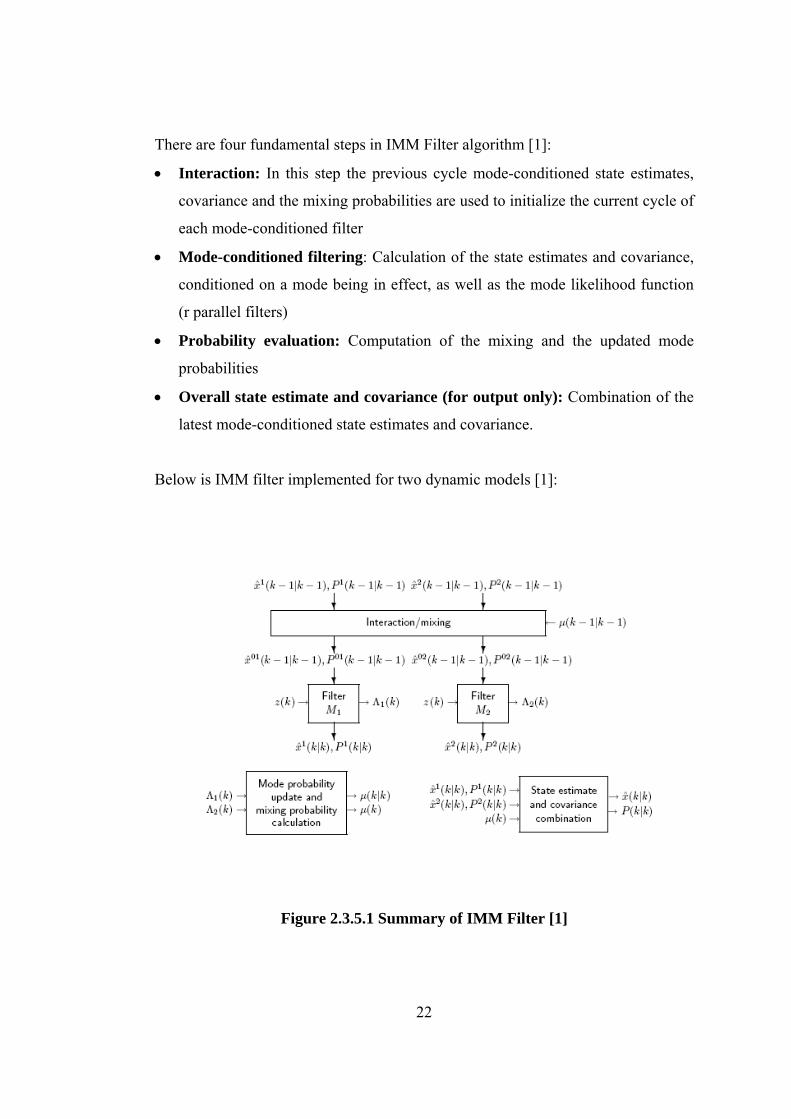
There are four fundamental steps in IMM Filter algorithm [1]:
• Interaction: In this step the previous cycle mode-conditioned state estimates,
covariance and the mixing probabilities are used to initialize the current cycle of
each mode-conditioned filter
• Mode-conditioned filtering: Calculation of the state estimates and covariance,
conditioned on a mode being in effect, as well as the mode likelihood function
(r parallel filters)
• Probability evaluation: Computation of the mixing and the updated mode
probabilities
• Overall state estimate and covariance (for output only): Combination of the
latest mode-conditioned state estimates and covariance.
Below is IMM filter implemented for two dynamic models [1]:
Figure 2.3.5.1 Summary of IMM Filter [1]
22

23
In this thesis, 2-model and 3-model IMM Filters are implemented. In 2-model IMM
Filter, Constant Velocity and Constant Acceleration Kalman Filters are used. In 3-
model IMM Filter, besides filters in 2-model IMM Filter, stationary target model is
added, which can be applicable to land targets.
CHAPTER 3
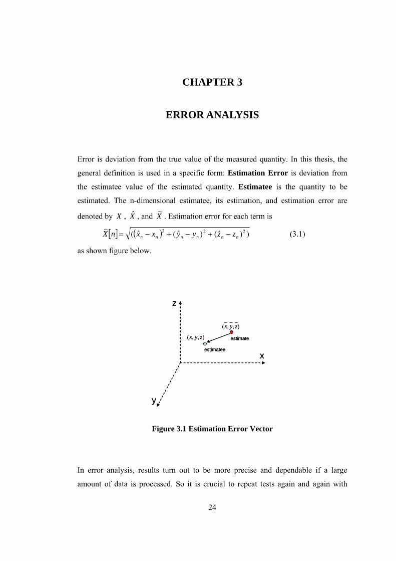
ERROR ANALYSIS Error is deviation from the true value of the measured quantity. In this thesis, the
general definition is used in a specific form: Estimation Error is deviation from
the estimatee value of the estimated quantity. Estimatee is the quantity to be
estimated. The n-dimensional estimatee, its estimation, and estimation error are
denoted by X , X , and X~ . Estimation error for each term is
[ ] ( ) ))ˆ()ˆ(ˆ(~ 222nnnnnn zzyyxxnX −+−+−= (3.1)
as shown figure below.
),,( zyx
),,( zyx
x
y
z
estimate
estimatee
),,( zyx
),,( zyx
x
y
z
estimate
estimatee
Figure 3.1 Estimation Error Vector
In error analysis, results turn out to be more precise and dependable if a large
amount of data is processed. So it is crucial to repeat tests again and again with
24

Monte-Carlo simulations. Here the total number of independent Monte-Carlo
simulations is denoted by M.
3.1 Root Mean Square Error - RMSE
∑ ∑= =
==M
i
M
iiii XX
MX
MXRMSE
1 1
21'2
12
2)~~1()~1()~( (3.1.1)
Root-Mean-Square Error (RMSE) is a widely used measure of estimation accuracy.
The popularity of RMSE comes from the fact that is it is older than the other
methods discussed below. RMSE is finite-sample approximation of the standard
error [ ]XXE ~~ ' , which is closely related with standard deviation. [11] Standard
deviation is an important parameter for probabilistic analysis, so RMSE is.
It is clear that smaller RMSE means a more accurate estimator.
3.2 Average Euclidean Error – AEE
∑ ∑= =
==M
i
M
iiii XX
MX
MXAEE
1 1
21'
2)~~(1~1)~( (3.2.1)
Average Euclidean Error (AEE) arises from Euclidean distance or Euclidean norm
[11]. AEE is finite-sample approximation of mean error [ ]2
~XE , which is in other
words mean deviation. Since mean deviation is never larger than standard deviation,
AEE is never larger than RMSE.
Again, smaller AEE means a more accurate estimator.
3.3 Geometric Average Error – GAE
M
iiMi XXXGAE
12
1'1 )~~()~( ⎥⎦
⎤⎢⎣⎡∏= = (3.3.1)
It is obvious that geometric average is never larger than arithmetic average, which is
never larger than the RMS value, GAE≤AEE≤RMSE. [11] GAE is useful to see the 25

existence of instantaneous large error. This is helpful to analyze the behavior of
filter with a maneuvering target. The estimation error increases when a straight
moving target begins to maneuver instantly, since it takes time for filter to update
its parameters.
Smaller GAE means a more accurate estimator.
3.4 Normalized Error In a radar tracking system, one of the main error sources is measurement error,
stemming from the sensor itself. To simplify the discussion, let us consider a two-
dimensional case of measurement from a sensor where ‘r’ and ‘a’ stands for range
and azimuth angle respectively:
a
r
x
ytarget
sensor a
r
x
ytarget
sensor
Figure 3.4.1 Sensor Measurement Vector
In cartesian coordinate;
( )arx cos= (3.4.1)
( )ary sin= (3.4.2)
assuming there is error both on range and angle measurement (r + Δr) and (a + Δa).
( ) ( )aarrxx Δ+Δ+=Δ+ cos (3.4.3)
26

( ) ( )aarryy Δ+Δ+=Δ+ sin (3.4.4)
Taking equation 3.4.3 and using trigonometric identities,
( )[ ]aaaarrxx Δ−ΔΔ+=Δ+ sinsincoscos (3.4.5)
for small Δa using Taylor series expansion;
( ) 12
1cos2
≈Δ
+≈Δaa (3.4.6)
( ) aaaa Δ≈Δ
−Δ≈Δ!3
sin3
(3.4.7)
Putting Equations 3.4.6 and 3.4.7 into Equation 3.4.5
( )[ aaarrxx ]Δ−Δ+=Δ+ )(sincos (3.4.8)
araraaararxx ΔΔ−Δ+ΔΔ−=Δ+ )(sin)(cos)(sincos (3.4.9)
Where
arx cos= (3.4.10)
aarrax ΔΔ−Δ=Δ )(sin)(cos (3.4.11)
0)(sin ≈ΔΔ ara (3.4.12)
As seen in equation 3.4.11, for small aΔ and rΔ , dominant figure in measurement
error is proportional to range. To make error measure independent of trajectory,
each error must be normalized with the range where error is calculated. Normalized
error at sample i in a trajectory is given by
i
ii r
xne
~= (3.4.15)
NE is n dimensional normalized error of a trajectory. NE is applicable to RMSE,
AEE, and GAE error measures. Instead of X~ , NE can be put into related equations.
∑ ∑= =
==M
i
M
iiii NENE
MNE
MXRMSENormalized
1 1
21'2
12
2)1()1()~( (3.4.13)
∑ ∑= =
==M
i
M
iiii NENE
MNE
MXAEENormalized
1 1
21'
2)(11)~( (3.4.14)
M
iiMi NENEXGAENormalized
12
1'1 )()~( ⎥⎦
⎤⎢⎣⎡∏= = (3.4.15)
27

Besides normalizing error measures, it can be helpful to make error analysis
independent of trajectory length. Making error analysis independent of trajectory,
we gain the possibility of using error measure as specification of a tracking system.
For this, each normalized error analysis results can be divided into total number of
samples for each Monte Carlo simulation (let us take number of samples: ‘k’) as
shown below.
kMXRMSENormalizedXSErmalizedRMgthIndepNoTrajectLen /)~()~( = (Eq.3.4.16)
kMXAEENormalizedXErmalizedAEgthIndepNoTrajectLen /)~()~( = (Eq.3.4.17)
kMXGAENormalizedXErmalizedGAgthIndepNoTrajectLen /)~()~( = (Eq.3.4.18)
3.5 Error Measures for Video Trackers When dealing with video tracking, one will find himself in the 2D world. In most
video tracking systems, there two phases: Detection and Tracking. In detection
period, where image processing methods are used, probable targets are figured out.
In tracking period, where estimation filters are at work, one or few of probable
targets’ next position are estimated. Therefore, in finding error measures for video
trackers, we have to take into account both image processing and estimation filter.
Most of the time, the gravity centre of target’s 2D image is ordered to track. In
minor cases, the edge of a target is the interest of tracking filters. From this point of
view, center of gravity of target image will be used as reference data to find out
estimation error. To find out the center of gravity of the target, one needs the exact
placement of target image in a series of frames, which is called ‘Ground Truth’.
To simplify the problem, it is enough to take the quadrangle window (‘Ground
Truth Window’) frame that each edge touches to the target. Ground truth of the
target is shown in Figure 3.5.1
28

Target’s center of gravity (Ground Truth)
Estimation output
Estimation errorGround Truth Window
Target’s center of gravity (Ground Truth)
Estimation output
Estimation errorGround Truth Window
Fig. 3.5.1 Ground Truth and Ground Truth Window
3.5.1 Probability of Detection
In video tracking systems, it is essential that estimation falls in Ground Truth
Window. Estimation is used to place detection window where target will be found
out in the next frame. If estimation is out of Ground Truth Window, then detection
window should be placed where another irrelevant target takes place. Probability of
estimation being in the Ground Truth Window is called ‘Probability of Detection’.
Sometimes Probability of Detection is used to define how accurate that target is
distinguished from the background in the detection phase of video tracking.
However, taking video tracking -detection and tracking phases- as a whole system,
detection and estimation errors are evaluated together. Probability of detection is
the best when it is 100%. Specification of a video tracking system, can be given in
terms of Probability of Detection.
Probability of = (Number of frames that estimation falls in Ground Truth
Detection Window / number of total frames under test) x 100
29

3.5.2 Degree of Vicinity
Another essential item in video tracking error analysis is how close estimations are
to Ground Truth, which can be called as ‘Degree of Vicinity’. Here again both
detection and estimation errors are evaluated together. In some cases, it is
acceptable to track a target with a constant deviation. This constant deviation can be
large enough to put estimation out of the Ground Truth Window. In such a case,
system itself can assign a constant to take estimation in Ground Truth Window.
Every system is designed with a limit before braking down, so it is crucial to know
the closeness of estimation to ground truth before giving up track.
Let us call error between estimation and Ground Truth as error and diagonal length
of Ground Truth Window as diagonal. Degree of Vicinity can be formulized as
21
2
2 ⎟⎟⎟⎟
⎠
⎞
⎜⎜⎜⎜
⎝
⎛
⎟⎟⎟
⎠
⎞
⎜⎜⎜
⎝
⎛= ∑ diagonal
errorDoV (3.5.2.1)
As it can be guessed, smaller DoV means a better video tracker system.
30

31
CHAPTER 4
RESOURCE ANALYSIS When implementing any algorithm into hardware, there are resource requirements
in terms of memory and processing power. One must take these into account, when
choosing the processor platform and amount of memory. Another issue about
hardware implementation is the complexity of algorithm related to the size of
Programmable Logic Cell Arrays.
However, the hardware implementation of an algorithm must be considered as a
part of system itself, not stand alone. For example, in a multi-target tracking system,
the amount of memory requirement increases geometrically as the number of targets
increases. Besides, if there is a real time requirement of the system, then all
resources must be revised again, e.g. parallel processing.
As mentioned before, five fundamental estimation filters and their variations are
investigated in this thesis:
• Alpha-Beta
• Alpha-Beta-Gamma
• Kalman – Constant Velocity
• Kalman – Constant Acceleration
• Extended Kalman Filter
• 2-model IMM Filter
• 3-model IMM Filter
In the next sub-sections; the memory requirement, processing power, and algorithm
complexity of above filters are discussed for single target tracking with one sample
estimation.

32
4.1 Memory Requirement The memory requirements of filters are examined in relation to the number of
constant, variable and temporal values used in the algorithms.
• Constants: These values are used without any change during execution of
algorithm
• Variables: These values change from one data set (e.g. estimation) to the
other.
• Temporal: These values are intermediate values which are not directly
related to filter constructers
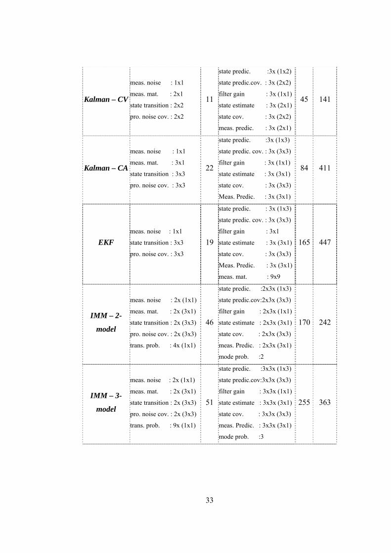
In the table below, memory requirements are given for estimation filters. When
evaluating filters by their memory requirements, total constants and total variables
are summed up to find out total memory needs. As its is guessed the memory
requirements of filters increase in the following order: Alpha-Beta, Alpha-Beta-
Gamma, Kalman – Constant Velocity, Kalman – Constant Acceleration, Extended
Kalman Filter, 2-model IMM Filter and 3-model IMM Filter.
Table 4.1.1 Memory Requirements of Fundamental Estimation Filters
Estimation
Filter Constants
Tot.
cons.Variables
Tot.
var. Temp.
Alpha-Beta alpha : 1x1
beta : 1x1
T : 1x1
3 position : 3x (1x1)
velocity : 3x (1x1) 6 12
Alpha-Beta-
Gamma
alpha : 1x1
beta : 1x1
Gamma : 1x1
T : 1x1
T^2 : 1x1
5 position : 3x (1x1)
velocity : 3x (1x1)
acceleration : 3x (1x1)
9 24
33
Kalman – CV
meas. noise : 1x1
meas. mat. : 2x1
state transition : 2x2
pro. noise cov. : 2x2
11
state predic. :3x (1x2)
state predic.cov. : 3x (2x2)
filter gain : 3x (1x1)
state estimate : 3x (2x1)
state cov. : 3x (2x2)
meas. predic. : 3x (2x1)
45 141
Kalman – CA
meas. noise : 1x1
meas. mat. : 3x1
state transition : 3x3
pro. noise cov. : 3x3
22
state predic. :3x (1x3)
state predic. cov. : 3x (3x3)
filter gain : 3x (1x1)
state estimate : 3x (3x1)
state cov. : 3x (3x3)
Meas. Predic. : 3x (3x1)
84 411
EKF meas. noise : 1x1
state transition : 3x3
pro. noise cov. : 3x3
19
state predic. : 3x (1x3)
state predic. cov. : 3x (3x3)
filter gain : 3x1
state estimate : 3x (3x1)
state cov. : 3x (3x3)
Meas. Predic. : 3x (3x1)
meas. mat. : 9x9
165 447
IMM – 2-
model
meas. noise : 2x (1x1)
meas. mat. : 2x (3x1)
state transition : 2x (3x3)
pro. noise cov. : 2x (3x3)
trans. prob. : 4x (1x1)
46
state predic. :2x3x (1x3)
state predic.cov:2x3x (3x3)
filter gain : 2x3x (1x1)
state estimate : 2x3x (3x1)
state cov. : 2x3x (3x3)
meas. Predic. : 2x3x (3x1)
mode prob. :2
170 242
IMM – 3-
model
meas. noise : 2x (1x1)
meas. mat. : 2x (3x1)
state transition : 2x (3x3)
pro. noise cov. : 2x (3x3)
trans. prob. : 9x (1x1)
51
state predic. :3x3x (1x3)
state predic.cov:3x3x (3x3)
filter gain : 3x3x (1x1)
state estimate : 3x3x (3x1)
state cov. : 3x3x (3x3)
meas. Predic. : 3x3x (3x1)
mode prob. :3
255 363

0
50
100
150
200
250
300
350
Alpha-B
eta
Alpha-B
eta-G
amma
Kalman
- CV
Kalman
- CA
EKF
IMM - 2
mod
el
IMM - 3
mod
el
Mem
ory
Req
uire
men
ts
Figure 4.1.1 Memory Requirements of Fundamental Estimation Filters
4.2 CPU Usage When implementing any algorithm in hardware with real-time requirement, one of
the primary questions to be answered is ‘Is this hardware fast enough to handle this
algorithm?’ Answer to this question may be found in two ways:
• Each arithmetic operator to be executed in algorithm can be counted,
number of operators gives total CPU usage. In a conventional CPU, each
type of arithmetic operator lasts differently, i.e. division lasts longer than
summation.
• Another method to find out CPU usage is to put algorithm into CPU, and
measure CPU time. In this thesis, this method is used, algorithms are
implemented in MATLAB. Codes below are used to calculate CPU time in
MATLAB [12].
34…

35
cputime;
);
CPU usage of estimation filters investigated in this thesis are examined below. For
The Alpha-Beta filter is taken as basis to compare the CPU usage of estimation
filters. Below is CPU usage of estimation filters discussed in this thesis. The results
are gathered from six different trajectories and several Monte Carlo simulations.
t =
surf(peaks(40)
e = cputime-t
e = 0.4667
…
CPU time calculation, the execution priority of the MATLAB is made ‘Realtime’ to
avoid CPU being blocked by other application. During simulations, the
configuration of PC is Pentium M Centrino 1300MHz CPU and 512MB RAM.
Figure 4.2.1 Making MATLAB a Real-time Application in Windows OS

36
or
ATLAB to distinguish from each other.
r implementation and again resolution of
ATLAB. While implementing both filters, same filter constructers are used,
odel IMM filter.
Figure 4.2.2 CPU Usage of Estimation Filters
It can be seen that Alpha-Beta and Alpha-Beta-Gamma filters’ CPU usage are close
to each other. The order of CPU usage for these filters is 10-4, which is very low f
M
Constant Velocity and Constant Acceleration Kalman filter’s CPU usage are also
close to each other. This is because of thei
M
except zeros are put into matrices since Constant Velocity Kalman filter does not
use these values. However, it is still acceptable that CPU usage of these two filters
is close to each other.
As expected, the CPU usage of other filters are arranged in ascending order as EKF,
2-model IMM and 3-m
Alpha-B
eta
Alpha-B
eta-G
amma
Kalman
- CV
Kalman
- CA
EKF
IMM - 2
mod
el
IMM - 3
mod
el
CPU
Usa
ge
37
les
. When the sizes of matrices increase by r rows and c columns
(i.e. ), the number of operations to multiply two matrices will
incre
4.3 Algorithm Complexity Algorithm Complexity is somehow a qualitative measure which depends on
implementation of the algorithm. In this thesis, Algorithm Complexity is defined
as the density of intermediate calculations and the number of matrices and variab
used in the algorithm.
Let us assume that an algorithm will be implemented on a Programmable Logic
Cell Array (PLCA). As the number of the intermediate calculations increases, the
area used on a PLCA will increase. As an example, we multiply two matrices with
size aa×
)()( cara +×+
ase by crcbcar −++ 222 .However, the number of cells in both matrices
increases by +r
In such a qualitative evaluation, it is bet pare algorithm complexities of
he lowest density of intermediate calculation is
ediate calculation; however the number of matrices and
ariables in CA Kalman filter is larger than matrices in CV Kalman filter. The
ously, 3-mode
this discussion, th
Alpha-Bet amma, CV Kalman, CA Kalman, EKF, 2-model IMM
nd 3-model IMM.
22 −c . 2
ter to com
filters with each other one by one. T
in Alpha-Beta filter, which is followed by Alpha-Beta-Gamma filter. Since each
parameter and coordinate value is calculated separately, the number of matrices and
variables used in both filters are nearly same. CV and CA Kalman filters have the
same number of interm
v
construction of EKF is nearly the same as the CA Kalman filter, however there are
linearization operations which add extra variables and intermediate calculations. 2-
model IMM filter has more intermediate calculation than EKF. As the number of
models used in IMM filter increases, number of intermediate operations ramp up.
Obvi l IMM filter has much more operations than any of the filters
above. From e filter complexity increases in the following order:
Alpha-Beta, a-G
a

38
Figure 5.1 Simulation User Interface
CHAPTER 5
SIMULATIONS MATLAB is chosen as the simulation tool, because of its flexibility in
mathematical environment. In the simulations, estimation filters discussed in
Chapter 2 are implemented. For error analysis, error measures in Chapter 3 (except
section 3.5) are coded. A user interface is designed to change inputs to the filters
and to monitor the outputs. In order to test implemented filters, benchmark
trajectories given in the literature [13] are used.

39
By the simulation user interface, trajectory data as measurement
ata and the number of Monte Carlo simulations. When the RUN button is pressed,
e chosen trajectory is fed to all estimation filters implemented: Alpha-Beta,
Alpha-Beta-Gamma, CV Kal 2-model IMM and 3-model
M filters. The results collected from filter output and trajectory data are used to
alculate error metrics: RMSE, AEE, GAE and normalized error (trajectory length
.1 Trajectory Test Data this thesis 6 different trajectories are used which are taken from Blair,W.D.,
atson,G.A., Kirubarajan, T., and Bar-Shalom,Y., et al, “Benchmark for Radar
the user can choose
d
th
man, CA Kalman, EKF,
IM
c
independent normalized error). The elapsed time of each filter is displayed
individually. The user can examine the error distribution of each filter separately.
The mean and variance of the error distributions are also displayed. The results of
filters can be displayed together with the trajectory.
5In
W
Allocation and Tracking in ECM” [13].
5.1.1 Trajectory – 1 The target flies with constant speed of 290 m/s at an altitude of 1.26 km for the first
60 s. Then, it turns with 2 g acceleration and flies with constant speed for another
30 s. Then, it turns with 3 g and flies to its final range. This trajectory simulates a
large aircraft. The trajectory is shown below:

40
Figure 5.1.1.1 Trajectory – 1
5.1.2 Trajectory – 2 The target flies with constant speed of 305 m/s at an altitude of 4.57 km for the first
60 s. Then, it turns 2/π with 2.5 g acceleration and descends to 3.05 km. Then, it
turns with 4 g and flies to its final range with constant speed of 305 km/s. This
trajectory represents a small maneuverable commercial jet. The trajectory is shown
below:
41
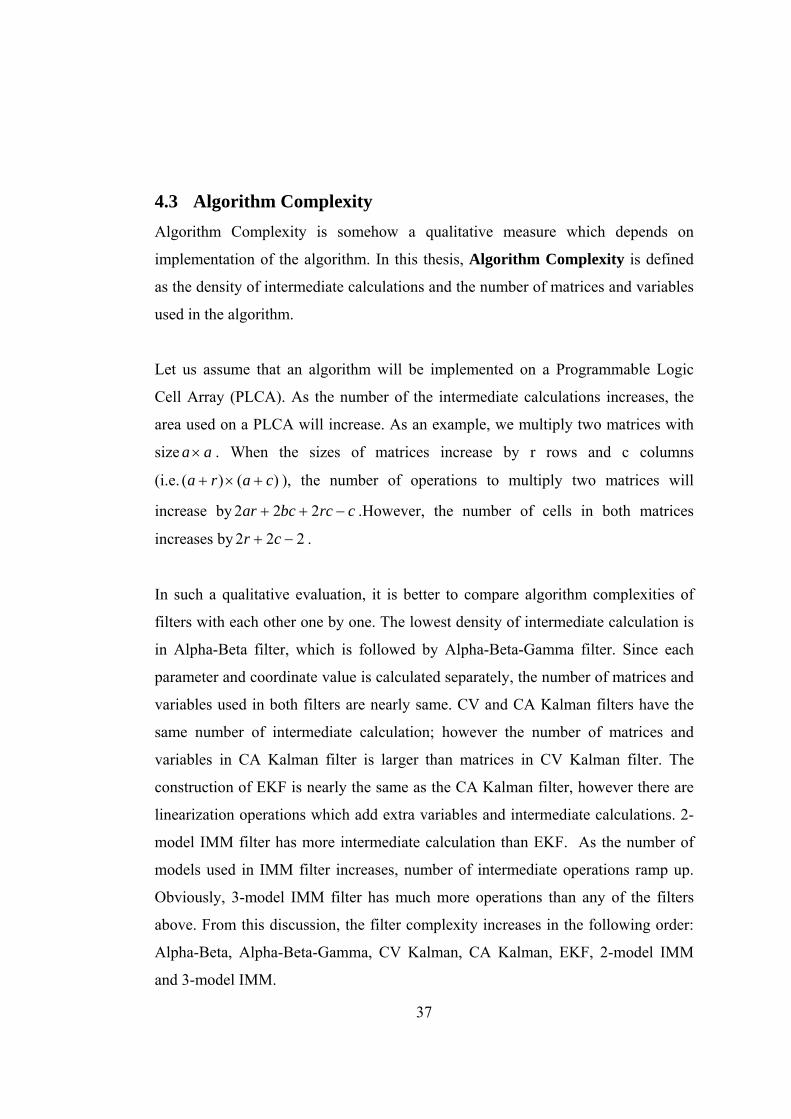
Figure 5.1.2.1 Trajectory – 2
5.1.3 Trajectory – 3 The target flies with constant speed of 457 m/s for the first 30 s. Then, it turns 4/π
with 4 g acceleration and it flies with a constant speed for another 30 s. Then, it
with 4 g and decreases its speed to 274 m/s. With this speed it flies to its turns 2/π
final range. This trajectory represents a medium bomber. The trajectory is shown
below:

Figure 5.1.3.1 Trajectory – 3
5.1.4 Trajectory – 4 The target flies with constant speed of 251 m/s at an altitude of 2.29 km for the first
30 s. Then, it turns 4/π with 4 g acceleration and flies with constant speed for
another 30 s. Then, it turns with 6 g and ascends to 2.9 km. It flies with constant
speed to its final destination. This trajectory again represents a medium bomber.
The trajectory is shown below:
42

43
Figure 5.1.4.1 Trajectory – 4
ectory with acceleration at an altitude of 1.5 km. For the
5.1.5 Trajectory – 5 The target begins its traj
first 30 s it flies with constant acceleration. Then, it turns with 5 g and flies with
constant speed for another 20 s. Then, it turns with 7 g and flies with constant speed
for 30 s. After flying with constant speed, it turns with 6 g. After reaching at
altitude of 4.45 km, it flies with a constant speed horizontally. This trajectory
represents a fighter. The trajectory is shown below:

44
Figure 5.1.5.1 Trajectory – 5
nal destination. This trajectory
represents a fighter, too. The trajectory is shown below:
5.1.6 Trajectory – 6 The target flies with constant speed of 426 m/s at an altitude of 1.55 km for the first
30 s. Then, it turns with 7 g and flies with constant speed for another 30 s. Then, it
turns with 6 g and descends until altitude of 0.79 km. It flies with a constant speed
for 30 s and then it turns with 6 g. Another constant speed flight is performed until 7
g turn. Then it flies with constant speed to its fi

Figure 5.1.6.1 Trajectory – 6
45
e of each filter.
One another useful information for error analysis is the distribution of error. The
frequency of each error value is put on plot where y-coordinate is repetition number
of error and x-coordinate is value of error, yielding the Error Distribution. Mean
and variance of Error Distribution are helpful statistical information for error
analysis.
5.2 Simulation Results Each trajectory is fed to estimation filters as measurement data and estimation
results of estimation filters are collected in separate arrays. From trajectory data and
estimation filter’s results, the error at each sample is calculated. By using error at
each sample, error measures are calculated according to methods discussed in
Chapter 3 (except subsection 3.5). Besides, elapsed time to process a trajectory by
an estimation filter is calculated to find out the CPU usag

46
In order to make simulation results more trustable, Monte Carlo simulation method
is used. Each trajectory is fed to the estimation filters several times with different
random noise added to the original data. Each result is taken individually to
calculate error measures. There is a trade-off between time consumption and
reliability of tests conducted. Here, the degree of the Monte Carlo is 3, which means
that the trajectory data is fed to estimation filters 3 times with different random
noise each time.
5.2.1 Trajectory – 1
he first trajectory is fed to the filters, and the above results are obtained. As can be
an maneuverable motion. CA Kalman filter is as bad as Alpha-Beta and
lpha-Beta-Gamma filters, because it is sensitive to acceleration but it is not
successful for motion with constant velocity. 2-model IMM is better than CA
Figure 5.2.1.1 Simulation Results for Trajectory-1
T
seen, EKF gives the best result, where lowest error value means that the estimation
filter output is closest to the measurement data. Actually, this is as expected since
EKF is more sensitive to maneuverable behavior and accelerated turn. CA Kalman
filter is worse than CV Kalman filter, due to the fact that constant velocity motion
is more th
A

47
IMM filter uses CP Kalman model which causes to increase error
te.
the average elapsed time in ascending order are: Alpha-
e to
Kalman and CV Kalman filters, which is acceptable since 2-model IMM has the
flexibility of both CA Kalman and CV Kalman filters. With this approach, it is
expected that 3-model IMM should give better results than 2-model IMM. Besides
CV Kalman and CA Kalman filters, Constant Position (CP) Kalman filter is used as
third model. Since trajectory-1 is a moving target, in some cases (even the
probability of being in CP Kalman model or change into CP Kalman model is kept
smaller) 3-model
ra
The filters according to
Beta, Alpha-Beta-Gamma, CV Kalman, CA Kalman, EKF, 2-model IMM and 3-
model IMM. The elapsed time for Alpha-Beta filter seems to be zero, this is du
the fact that the minimum sensible resolution is smaller than elapsed time.
Figure 5.2.1.2 Error Distribution of Alpha-Beta Filter Output
Error distribution of Alpha-Beta filter shows that most of error terms are gathered
around 0.0603 with variance 0.0001.
48
ilter’s,
athered around 0.0604 with variance 0.0001. Variance is a little higher, since
lpha-Beta-Gamma reacts to changes slower than the Alpha-Beta filter, in case of
maneuvering target.
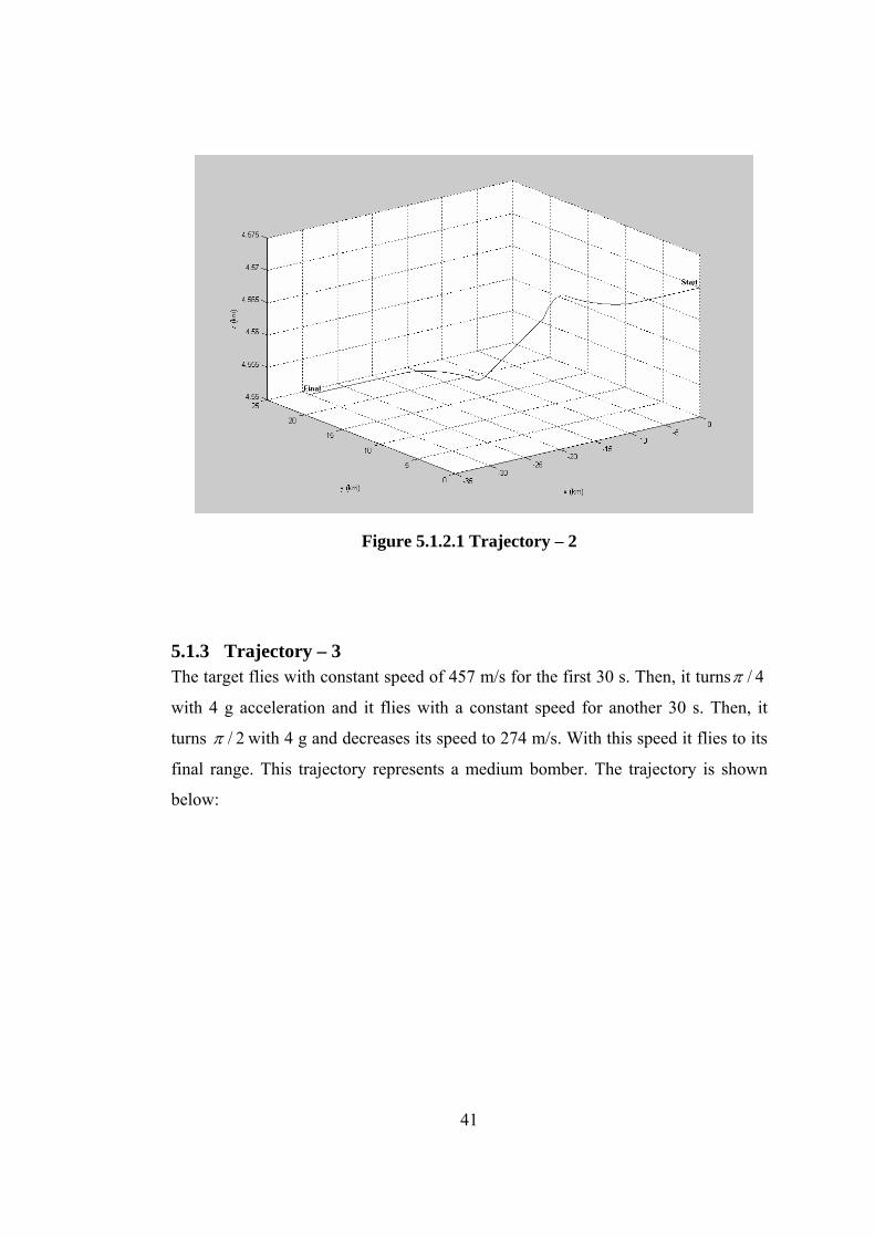
Figure 5.2.1.3 Error Distribution of Alpha-Beta-Gamma Filter Output
Error distribution of Alpha-Beta-Gamma filer is nearly same as Alpha-Beta f
g
A
Figure 5.2.1.4 Error Distribution of CV Kalman Filter Output

49
rror distribution values of CV Kalman filter are smaller than those of both filters
above. Mean is 0.0448 with variance of 0.0003. While error metric decreases,
variance increases. The estimated results are closer to the exact trajectory, however
the reaction of filter to changes of target maneuver is slower.
he mean of CA Kalman filter error distribution is 0.0563 with variance of 0.0005,
-
sed,
m
E
Figure 5.2.1.5 Error Distribution of CA Kalman Filter Output
T
which is larger than any of the values above. CA Kalman model is assuming that
most of the time target moves with acceleration, which is not the case for trajectory
1. Variance is larger, because of the fact that the degree of the filter is increa
eaning slower reaction to maneuver.

50
the
m
measure artesian
and spherical coordinate systems.
Figure 5.2.1.7 Error Distribution of 2-model IMM Filter Output
Figure 5.2.1.6 Error Distribution of EKF Output
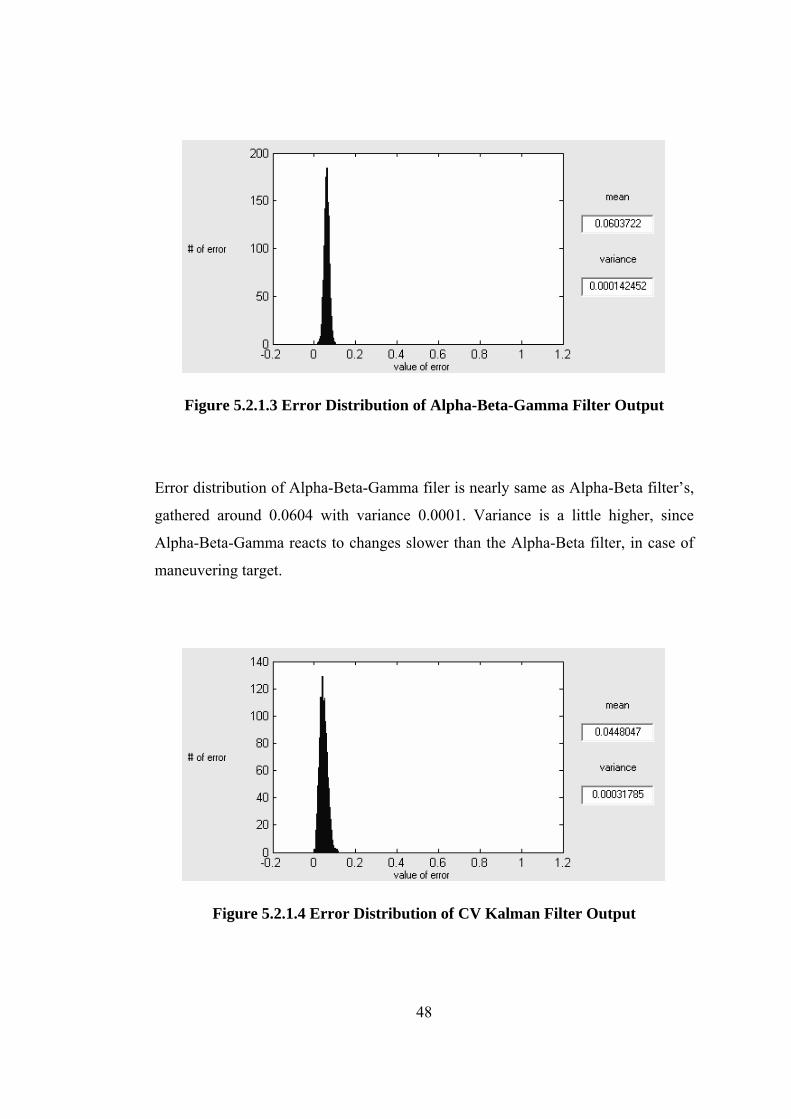
The error distribution of EKF output is interesting compared to the others. Mean is
0.0315 with variance 0.00009. It seems that all error terms are close to a single
point. This shows that there is a bias on error, which means that if we subtract
ean value from all error terms, the EKF estimation will be much closer to the
ment data. The source of this bias is the transformation between C
51
Mean of 2-model IMM filter’s error distribution is 0.0328 with variance 0.00016.
The means of the 2-model IMM filter’s error distribution (0.0315) and EKF’ error
distribution are very close to each other, while error metrics RMSE, AEE and GAE
are slightly different. This shows that it may not be proper to use mean of error
terms directly. It is useful to put them in a meaningful format to examine.
he error distribution of 3-model IMM filter output’s mean is 0.0401 and variance
ial
Figure 5.2.1.8 Error Distribution of 3-model IMM Output
T
is 0.00019. The mean and variance are larger than 2-model IMM filter’s, because
of 3rd model (Constant Position model), which is much applicable to terrestr
targets.

5.2.2 Trajectory – 2
52
Figure 5.2.2.1 Simulation Results for Trajectory-2
As in Trajectory-1, the order of filters in terms of error metrics are as follows :
Alpha-Beta,
model IMM and EKF. Also the order of the filter process elapsed time is the same
as above, however time is increased. This is because of the increase in target
Alpha-Beta-Gamma, CA Kalman, CV Kalman, 3-model IMM, 2-
maneuver.

53
Figure 5.2.2.2 Error Distribution of Alpha-Beta Filter Output
d 0.00014 of
ariance.
Figure 5.2.2.3 Error Distribution of Alpha-Beta-Gamma Filter Output
The error distribution of Alpha-Beta filter has mean of 0.0632 an
v
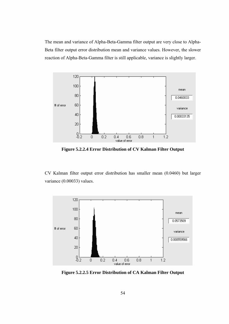
54
The mean and variance of Alpha-Beta-Gamma filter output are very close to Alpha-
Beta filter output error distribution mean and variance values. However, the slower
reaction of Alpha-Beta-Gamma filter is still applicable, variance is slightly larger.
igure 5.2.2.4 Error Distribution of CV Kalman Filter Output
Figure 5.2.2.5 Error Distribution of CA Kalman Filter Output
F
CV Kalman filter output error distribution has smaller mean (0.0460) but larger
variance (0.00033) values.

As in trajectory-1, trajectory-2 has also constant velocity motion most of time,
which decreases performance of the CA Kalman filter. Mean is 0.0574 and variance
55
0.00056.
possible to subtract mean (0.0339) from all error terms
to remove biasing.
Figure 5.2.2.7 Error Distribution of 2-model IMM Filter Output
is
Figure 5.2.2.6 Error Distribution for EKF Output
Error distribution of EKF output is the same as before, error terms are collected
around one value. It is still

56
, respectively.
Figure utput
– 3
The mean and variance of 2-model IMM filter output error distribution is 0.0336
and 0.00017
5.2.2.8 Error Distribution of 3-model IMM Filter O
The mean is 0.0418 and the variance is 0.00022, which are larger than above.
5.2.3 Trajectory
Figure 5.2.3.1 Simulation Results for Trajectory-3

57
ers form worse to better is: Alpha-Beta, Alpha-Beta-
Gamma, CA Kalman, CV Kalman, 3-model IMM, EKF and 2-model IMM. The
roles of 2-model IMM filter and EKF seems to be changed, however in Figure
5.2.3.6 there is still bias on EKF output error terms. If this biasing is canceled out,
then EKF will give the best result. The value of biasing is related to the coordinate
transformation, and the cancellation value should be defined during this
transformation.
Figure 5.2.3.2 Error Distribution of Alpha-Beta Filter Output
The mean and variance of Alpha-Beta-Gamma filter output error distribution are
0.0927 and 0.00015, respectively.
For this trajectory, 2-model IMM filter gives the best result in terms of error
metrics. The order of filt

58
Alpha-Beta-Gamma Filter Output
For trajectory-3, the mean and variance values of Alpha-Beta-Gamma are nearly
same as in Alpha-Beta.
ribution of CV Kalman Filter Output
The mean and variance of CV Kalman filter output’s error distribution is 0.0563
and 0.00039, respectively.
Figure 5.2.3.3 Error Distribution of
Figure 5.2.3.4 Error Dist

59
Figure 5.2.3.5 Error Distribution of CA Kalman Filter Output
of CV Kalman filter output’s error distribution is 0.0658
nd 0.00067, respectively.
Figure 5.2.3.6 Error Distribution of EKF Output
The mean and variance
a

60
Bias on error terms is still effective, to cancel biasing mean value can be subtracted
Figure 5.2.3.7 Error Distribution of 2-model IMM Filter Output
he error distribution of 2-model IMM filter has mean of 0.0431 and variance of
.00019.
Figure 5.2.3.8 Error Distribution of 3-model IMM Output
from error terms.
T
0
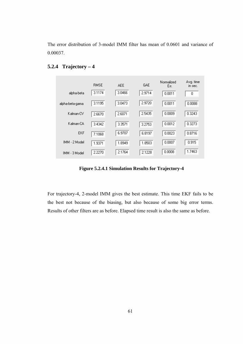
The error distribution of 3-model IMM filter has mean of 0.0601 and variance of
0.00037.
61
5.2.4 Trajectory – 4
Figure 5.2.4.1 Simulation Results for Trajectory-4
For trajectory-4, 2-model IMM gives the best estimate. This time EKF fails to be
the best not because of the biasing, but also because of some big error terms.
Results of other filters are as before. Elapsed time result is also the same as before.

62
Figure 5.2.4.2 Error Distribution of Alpha-Beta Filter Output
The mean and variance of Alpha-Beta filter output error distribution are 0.0529 and
0.00014, respectively.
Figure 5.2.4.3 Error Distribution of Alpha-Beta-Gamma Filter Output
The mean and variance of Alpha-Beta-Gamma filter output error distribution are
nearly the same as Alpha-Beta results.

63
Figure 5.2.4.4 Error Distribution of CV Kalman Filter Output
The error distribution of CV Kalman filter has mean of 0.0431 and variance of
0.00019.
Figure 5.2.4.5 Error Distribution of CA Kalman Filter Output
The error distribution of CV Kalman filter output has mean of 0.0431 and variance
of 0.00019.

64
at there are some big error terms that affect the variance value. Actually,
e mean of EKF output error distribution is 20% larger than the mean of 2-model
M filter output error distribution, while RMSE of EKF is 3.5 times larger than
Figure 5.2.4.7 Error Distribution of 2-model IMM Filter Output
Figure 5.2.4.6 Error Distribution of EKF Output
The mean of the error distribution of EKF output is 0.0518 with variance 0.0167. It
is clear th
th
IM
RMSE of 2-model IMM. RMSE emphasizes big error terms; it prevents big error
terms being canceled by small terms. This shows the benefit of using RMSE instead
of mean.

65
The error distribution of CV Kalman filter output has mean of 0.0312 and variance
of 0.00016.
istribution of CV Kalman filter output has mean of 0.0361 and variance
5.2.
Figure 5.2.4.8 Error Distribution of 3-model IMM Filter Output
The error d
of 0.00020.
5 Trajectory – 5
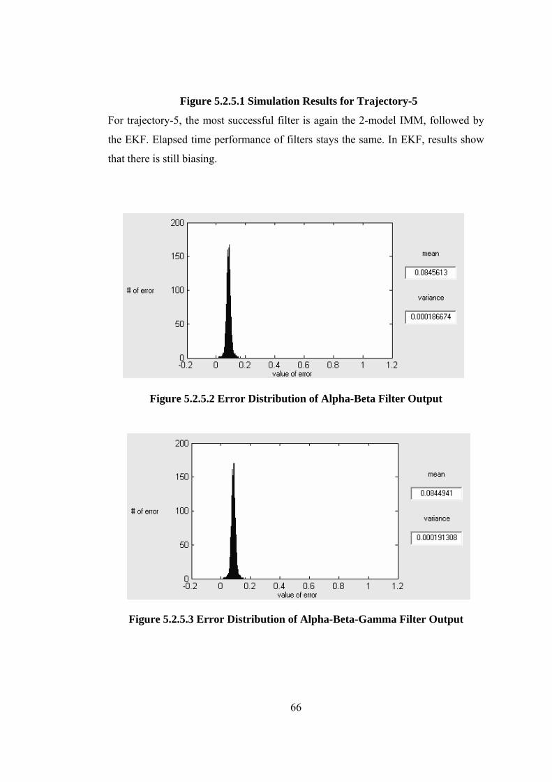
66
Figure 5.2.5.1 Simulation Results for Trajectory-5
psed time performance of filters stays the same. In EKF, results show
that there is still biasing.
Figure 5.2.5.2 Error Distribution of Alpha-Beta Filter Output
Figure 5.2.5.3 Error Distribution of Alpha-Beta-Gamma Filter Output
For trajectory-5, the most successful filter is again the 2-model IMM, followed by
the EKF. Ela

67
Figure 5.2.5.4 Error Distribution of CV Kalman Filter Output
Figure 5.2.5.5 Error Distribution of CA Kalman Filter Output

68
Figure 5.2.5.8 Error Distribution of 3-model IMM Filter Output
Figure 5.2.5.6 Error Distribution of EKF Output
Figure 5.2.5.7 Error Distribution of 2-model IMM Filter Output

69
5.2.6 Trajectory – 6
Figure 5.2.6.1 Simulation Results for Trajectory-6
In trajectory-6, the best estimate is given by the 2-model IMM filter, while CV
Kalman is the second best filter. 3-model IMM filter follows CV Kalman filter. If
biasing on EKF results are removed, the ranking can be changed in favor of EKF.
Ranking with respect to filter process elapsed time is the same as above.
Figure 5.2.6.2 Error Distribution of Alpha-Beta Filter Output

Figure 5.2.6.3 Error Distribution of Alpha-Beta-Gamma Filter Output
70
Figure 5.2.6.4 Error Distribution of CV Kalman Filter Output
t
Figure 5.2.6.5 Error Distribution of CA Kalman Filter Outpu

71
Figure 5.2.6.6 Error Distribution of EKF Output
Figure 5.2.6.7 Error Distribution of 2-model IMM Filter Output
Figure 5.2.6.8 Error Distribution of 3-model IMM Filter Output

72
5.3 ErThe selection of measurement noise covariance and process noise covariance
matrices has direct effect on performance of estimation filters: CV Kalman, CA
Kalman, EKF and IMM filters.
However, process noise covariance is adaptive during the filtering operation, until it
finally converges to a constant matrix in CA Kalman, CV Kalman and EKF. It will
be seen from the coming up simulation results that the initial condition of process
noise covariance is important, although it becomes stable regardless of
measurement data. In IMM filtering it stays adaptive during the complete process.
Process noise covariance matrix changes according to the target model used to
construc
The situation for the measurement noise covariance matrix is different. It stays
constant during the whole filtering process, which means that the initial choice is
important.
The four figures given below illustrate the relation between RMSE and
measurement noise covariance matrix coefficient. As the measurement noise
covariance matrix coefficient is changed, trajectory measurement data are fed to
filters for each measurement noise covariance matrix coefficient. The output of the
filter is collected
ror vs. Filter Constructers
t the filter.
to produce RMSE values individually.

73
Figure 5.3.1 RMSE vs. CV Kalman Filter Meas. Noise Cov. Matrix Coef.
The main aim is to make the RMSE value as small as possible, so for measurement
noise covariance matrix coefficient, the value around 1 and 3 is suitable for all
trajectories if CV Kalman filter will be used.

74
For E
value for all trajectories. For some trajectories it is around 2, however for some
trajectories it is around 9.
Figure 5.3.2 RMSE vs. CA Kalman Filter Meas. Noise Cov. Matrix Coef.
CA Kalman filter, there is no single range of values that decreases the RMS

Figure 5.3.3 RMSE vs. EKF Meas. Noise Cov. Matrix Coef.
75
variance matrix coefficient according to a single result
will degrade the error performance of the other trajectories.
For EKF, measurement noise covariance matrix coefficient can be chosen between
3.5 and 5. Only one trajectory shows that 1 is suitable to choose, however adjusting
the measurement noise co

76
Figure Coef.
SE and process noise
ovariance matrix. Trajectories are fed to filters for different process noise
covariance matrix coefficient. Each curve shows the results for a different
trajectory.
5.3.4 RMSE vs. 2-model IMM Filter Meas. Noise Cov. Matrix
For 2-model IMM filter, measurement noise covariance matrix coefficient can be
chosen between 3 and 5.
The four figures given below show the relation between RM
c

Figure 5.3.5 RMSE vs. CV Kalman Filter Proc. Noise Cov. Matrix Coef.
77
point according to the used target model regardless of
easurement data. Process noise covariance matrix coefficient can be chosen
.
For CV Kalman filter, process noise covariance matrix is adaptive during filtering,
until it reaches a stable
m
between 10 and 20. Since process noise covariance matrix reaches a stable point
regardless of measurement data, its best value can be found without measurement
data and initial condition can be chosen according to this value while filter is
constructed

Figure 5.3.6 RMSE vs. CA Kalman Filter Proc. Noise Cov. Matrix Coef.
For CA Kalman filter, a single process noise covariance matrix coefficient is not
possible, since for each trajectory minimum RMSE value has appeared at different
values. As in the case of measurement process noise covariance matrix, CA Kalman
is not a robust filtering method, which yields different results for different
trajectories.
78

Figure 5.3.7 RMSE vs. EKF Proc. Noise Cov. Matrix Coef.
For EKF, process noise covariance matrix can be chosen between 3 and 5.
79

80
Figure Coef.
uring all
filtering operation. This is because of the adaptive structure of IMM filtering. In
IMM filtering, which model is used with what percentage, is decided according to
the measurement data. The percentage of the model being used, determines process
noise covariance matrix structure. However, still the initial condition is effective on
RMSE value. For this simulation case, process noise covariance matrix coefficient
can be chosen between 2 and 9.
5.3.8 RMSE vs. 2-model IMM Filter Proc. Noise Cov. Matrix
In 2-model IMM filter case, process noise covariance matrix is adaptive d

81
CHAPTER 6
CONCLUSION In this thesis, the performance of 7 fundamental estimation filters is examined.
These are:
• Alpha-Beta
• Alpha-Beta-Gamma
• CV Kalman
• CA Kalman
• EKF
• 2-model IMM
Estimation filters are investigated with re ard to performance metrics and resource
e discussed.
RMSE and AEE are finite-sample approximation of standard error and mean error,
respectively [11]. AEE has a physical meaning while RMSE is a statistical term.
The physical meaning of AEE is the average distance between estimation and
measurement. RMSE is directly related to standard deviation. GAE prevents that
small errors are suppressed by large errors. In a radar system case, the order of the
error is related to range or in a video tracker system the order of error is related to
• 3-model IMM
g
requirement.
The aim of defining performance metrics is to put the error information in a more
usable and easily understandable format. In this thesis, four types of performance
metrics (RMSE, AEE, GAE and normalized from these) for general estimation
filters and two types of performance metrics (Probability of Detection and Degree
of Vicinity) for video trackers, ar

82
the size of the target. Therefore ful to normalize error terms to
ake error metric independent of range or target size.
Implementing an estimation f ssible by either software or
ardware or both. In all cases, it is essential to plan what kind of hardware is needed
run software or what kind of hardware is to be implemented. If there is real-time
ore crucial.
Res r n estimation filter can be defined in terms of CPU
usa s and complexity. In this thesis, fundamental estimation filters
are im MATLAB environment. In order to make an objective
com implementation the filter part of the MATLAB code is kept as
sim rder to measure the CPU usage of an estimation filter, CPU
tim f er is recorded. However, it is assured that there is no other
task disturbing CPU. Estimation filters arranged in order according to their CPU
alman, CA Kalman, EKF, 2-model IMM and 3-model IMM.
, it is more meaning
m
ilter into a system is po
h
to
requirement and besides other tasks are pending, then managing the resources
becomes m
ou ce requirements of a
ge, memory need
plemented in
parison, during
ple as possible. In o
e o estimation filt
usage is similar to the historical appearance of filters: Alpha-Beta, Alpha-Beta-
Gamma, CV K
In order to understand memory needs; variables, constants and intermediate
variables in MATLAB code of each filter are counted. Each cell of matrices is taken
as an individual memory element. The result again exhibits a parallelism with the
historical picture: Alpha-Beta, Alpha-Beta-Gamma, CV Kalman, CA Kalman, EKF,
2-model IMM and 3-model IMM.
Complexity of an estimation filter is defined as the density of intermediate
calculations and variables. Estimation filters are examined according to their
complexity, and the result is not surprising (from less to more): Alpha-Beta, Alpha-
Beta-Gamma, CV Kalman, CA Kalman, EKF, 2-model IMM and 3-model IMM.

83
is needed. However, it is not
fficient to work with a single trajectory, since each filter may be successful for a
e to fit the target trajectory and during this time it swings
round measurement data. Alpha-Beta-Gamma filter behaves in a similar way as
re inaccurate, then EKF will diverge. To reduce
e probability of EKF to diverge, it is recommended to begin with a robust filter
el
M and 3-model IMM filters are implemented. In 2-model IMM filter, CV and
CA Kalman filters are used and its success can be seen from simulation results.
Evaluation of estimation filters according to their performance metrics is quite
subtle. For trustable results, a set of measurement data
su
specific scenario. Alpha-Beta filter is the simplest estimation filter with constant
gains. Because of its simplicity, it is very suitable for real-time applications.
However, as it is seen from the simulation results that Alpha-Beta filter gives the
worst results. Alpha-Beta filter is not fast enough to respond to changes when there
is maneuver. It takes tim
a
the Alpha-Beta filter, except that it responds to acceleration on target motion. This
makes Alpha-Beta-Gamma filter more sensitive to maneuver.
CV Kalman filter is better than both of the filters above. However, it is more
complex and uses more resources. CV Kalman filter is also better than CA Kalman
filter. This is because of the acceleration terms in CA Kalman filter. Acceleration
part of the CA Kalman filter makes it slower to give response to the maneuvering
target. When estimations proceed, it takes longer for CA Kalman filter to fit back to
the trajectory.
All the above filters process each Cartesian coordinate variation individually, which
make these filters weaker in spherical motions. In EKF, this problem is solved by
linearizing measurement function around the measurement. Therefore, in most of
cases, EKF will give the best result, assuming that the divergence problem of EKF
is solved. If the initial estimates a
th
(like Kalman filter), use this period to initialize the EKF then continue with EKF.
The best filter all among the others is IMM filter, which gives flexibility to change
target dynamic model according to the measurement data. In this thesis, 2-mod
IM

84
error level should be
vestigated. An estimation filter which matches these requirements will be ‘the
Although, 3-model IMM filter has more alternative dynamic models than the 2-
model IMM filter, it gives the worse results. This is because of dynamic models
used in the 3-model IMM: CV Kalman, CA Kalman and Constant Position (CP)
Kalman. Since trajectories are chosen from aircrafts, CP Kalman is not suitable for
this kind of targets. CP Kalman model is chosen consciously to show that increase
in resource requirements or complexity does not always imply the best
performance.
An estimation filter can be called ‘the best estimation filter’ only with respect to a
particular application. Therefore, before choosing an estimation filter, most
probable target dynamics, hardware resources and acceptable
in
best estimation filter’.

85
, Artech House, Norwood, 1993
] M.S. Grewal, and A.P. Andrews, “Kalman Filtering: Theory and Practice”, 2nd
plications”, Artech House, Boston, 2004
] D.A. Wilson, Analysis Of Tracking and Identification Characteristics Of
iverse Systems and Data Sources For Sensor Fusion, A Master Thesis, California,
001
] G. Welch, and G. Bishop, “An Introduction to Kalman Filter”, Transaction of
epartment of Computer Science University of North Carolina, Chapel Hill, 2002
] L.J. Levy, “The Kalman Filter: Navigation's Integration Workhorse”,
ransaction of Applied Physics Laboratory of the Johns Hopkins University, 1997
] D. Simon, “Kalman Filtering”, Transaction of Innovative Software, 2001
] P.S. Maybeck, “Stochastic Models, Estimation and Control”, Academic Press
Inc., London, 1979
[10] R.E. Kalman, “A New Approach to Linear Filtering and Prediction Problems”,
Baltimore: Transactions of the ASME–Journal of Basic Engineering 82 (Series D):
35-45., 1960
[11] X.R. Li and Z. Zhao, “Practical Measures for Performance Evaluation of
Estimators and Filters”, Proceedings of the Workshop on Estimation, Monterey,
2001
[12] MATLAB User Guide Ver. 6.5 Relase 13, The MathWorks Inc., 2002
REFERENCES
[1] Y. Bar-Shalom, and X.R. Li, “Estimation and Tracking: Principles, Techniques,
and Software”
[2
Wiley Interscience, New York, 2001
[3] Y. Bar-Shalom and X.R. Li, “Multitarget-Multisensor Tracking: Principles and
Techniques”, YBS, Storrs, 1995
[4] B. Ristic, Arulampalam, S. and Gordon, N., “Beyond the Kalman Filter: Particle
Filters for Tracking Ap
[5
D
2
[6
D
[7
T
[8
[9

86
[13] W.D. Blair, G.A. Watson, T. Kirubarajan, and Bar-Shalom, “Benchmark for
Radar Allocation and Tracking in ECM”, IEEE Transactions on Aerospace and
Electronic Systems, Vol.34, No.4, October 1998
4] D.C. Montgomery, “Design and Analysis of Experiments”, 5th Ed., Wiley &
ons, Inc., New York, 2001
Tracking/Fusion Evaluation”, IEEE
“Practical Measures and Test for Credibility
-Shalom, Monterey, May 2001
. Brookner, “Tracking and Kalman Filtering Made Easy”, John Wiley & Sons
[1
S
[15] D.Y. Hsu, “Spatial Error Analysis”, IEEE Press, New York, 1999
[16] C.Y Chong, “Problem Characterization in
AESS Systems Magazine, p.12-17, July 2001
[17] X.R. Li, Z. Zhao and V.P. Jilkov,
of an Estimator”, Proceedings of the Workshop on Estimation, Tracking and
Fusion: A Tribute to Yaakov Bar
[18] D.R. Cox and N. Reid, “The Theory of the Design of Experiments”,
Chapman& Hall/CRC, New York, 2000
[19] S. Blackman and R. Popoli, “Design and Analysis of Modern Tracking
Systems”, Artech House, Nordwood, 1999
[20] E
Inc., New York,1998


