
1
1
Lec-02: Performance and Processor Architecture
ECE-720t4: Innovations in Processor Design
Mark Aagaard
2
Schedule01 Intro and Overview
02
03
04
05
06
07
08
09
10
11
12
13
Performance; Architecture
Pipelining review
Superscalar execution
Out-of-order execution: ctrl and data
Out-of-order execution: reordering
Processor Survey
Processor Trends
Data reuse and speculation
Multithreading concepts
Multithreading techniques
Review
PowerPC 620 vs Intel P6
In-orderexecution
O-o-Oexecution
Currentpractice
Recentadvances
3
Outline of Lecture• Historical definitions of performance • Amdahl’s law• “Iron law” of computer performance• Instruction set design• Pipelining• Instruction-level parallelism (not in lecture slides)
4
Outline of Chapter 1Processor Design
• 1.1 The Evolution of Microprocessors• 1.2 Instruction-Set Processor Design• 1.3 Principles of Processor Performance• 1.4 Instruction-Level Parallel Processing• 1.5 Summary

2
5
Origins of Measuring Performance• In early decades of computers, each new generation
required a new technique to evaluate performance.
Mid 1960s• Mainstream computers:
• had reasonably similar instruction sets• each instruction took same length of time to perform
• Performance measure: time to perform a single instruction (e.g. add)
6
Gibson Mix (1970)• Computers evolved so that some instructions took longer
to execute than others.• Gibson proposed: time to execute an average instruction,
based on weighted average of different instructions.
• Weights based on analyzing collection of typical programs
• Instruction frequency: static vs dynamic
7
Whetstone (1973)• Pipelining, caches, etc caused time to perform a single
instruction dependent upon instructions before and after.• Late 1960s: UK National Physical Laboratory
benchmarked programs using the Whetstone interpreter for Algol 60.
• 1971: portable benchmark with real programs was becoming too time consuming
• Whetstone: synthetic benchmark program• Relatively short (quick and easy to run)• Reflected distribution and order of typical scientific
program• Measure was KWIPS, then KMIPS, then MIPS
8
MIPS• MIPS = • Different types of MIPS
• Fastest instruction (e.g. NOP)• Typical instruction (e.g. ADD)• Weighted average (Gibson, Whetstone, Dhrystone)
• Advantages of MIPS:• simpler to explain to management• bigger is better.

3
9
Relative MIPS (1977)• IBM marketing claimed IBM 370/158 was (first?) 1MIPS
computer• DEC VAX 11/780 developers ran programs on IBM
370/158 and on VAX 11/780• Programs took same time on both computers,
therefore performance of VAX 11/780 was 1 MIPS• No one actually measured MIPS for VAX 11/780• VAX 11/780 become de facto standard for 1 MIPS
• 1981: Joel Emer from DEC measured VAX 11/780 as 0.5 MIPS
10
Dhrystone (1984)• Synthetic benchmark program• Focus on integer performance• Created by Reinhold Weicker (Seimens AG)
12
What Really Matters• The real definition of performance is how long it takes to
run your programs.
13
SPEC Benchmarks• Collection of real programs run for realistic lengths of time• Updated roughly every 5 years• Benchmarks for integer, floating point, graphics,
multiprocessors, Java client/server, mail servers, network file systems, web servers.
• spec.org: great resource before you buy your next computer!

4
14
Defining Equations for Performance
• To double performance• do the same amount of work in half the time• OR: do twice the work in the same amount of time
• Time is easy to measure• Challenge is to define or measure work• Benchmarketing is all about defining work to make your
product appear faster than your competitors’
TimeWorkPerformance
15
“Iron Law” of Performance
H&P , S&L 1.3
TimeProgram
InstrsProgram
CyclesInstr
TimeCycle
16
Tradeoffs
H&P , S&L 1.3.2
InstrsProgram
CyclesInstr
TimeCycle
17
Other Performance Equations
Speedup
n%faster
TSlowTFast
Speedup 1
1TSlowTFast
TSlowTFast
TFast
WeightedAvg ∑i=1
n%i × Ti

5
18
Example: Integer and Floating Point• Average time to execute an integer and floating-point
instruction on two computers:
CPU1CPU2
Int Float2.0ns 3.5ns2.5ns 3.0ns
• Q: Which CPU has greater performance for integer programs, and how much faster is it?
• Q: If the average program is 90% integer instructions and 10% floating-point instructions, which CPU has greater performance, and how much greater is the performance?
19
Example: Integer and Floating Point• Q: If we want to optimize the slower CPU to match the
performance of the faster CPU, should we optimize integer or floating-point instructions?
• Q: If you have to fire all of your computer architects because your stock price plummets, how can you get the slower CPU to match the performance of the faster CPU?
20
Amdahl’s Law• Supercomputers in 70s and 80s:
• multiple processors• scalar instructions: run on main processor• vector instructions: run on all processors
(useful for matrix and array operations)
Time
Act
ive
proc
esso
rs
Time
Act
ive
proc
esso
rs
100%
s
100% -- s
• Amdahl’s definition of efficiency
N
1×s + N×(100% -- s)N
21
Amdahl’s Speedup
1-ff
Time
Act
ive
proc
esso
rs
TFast
sN
TSlow
f = percentage of work done in vector mode100% -- f = percentage of work done in scalar mode
TFast = Time if have N processorsTSlow = Time if have just 1 processor
Speedup =

6
22
Amdahl and Pipelining
Time
Act
ive
stag
es
Time
Act
ive
stag
es
Time
Act
ive
stag
es
Time
Act
ive
stag
es
Affect of stalls:
23
Performance and Time• In the computer field, performance increases at an
exponential rate.• On average, doubles every 18 – 24 months.• Moore’s law says that number of available transistors
doubles every 18 – 24 months. • It’s up to the compiler writers, computer architects,
computer engineers, and electrical engineers to use the ever increasing number of transistors to improve performance.
• Equation for performance increasing by factor of n every k units of time:
P(t) = n(t/k)
24
Example: Perf. and Time to Market• Q: If performance doubles every 2 years, how much does
it increase each week?
• Q: You are considering a performance optimization that will delay your schedule by 4 weeks, but increase your performance by 5%, should you do the optimization?
25
Overview of Instruction Sets

7
26
Levels of Abstraction• ESL (electronic system level): several processors,
software, custom hardware. Software model of entire system to predict behaviour and performance.
• Transaction level: example transaction = (transfer packet from main-cpu to cryptography engine; encrypt; transfer packet back to main-cpu)
• ISA (instruction-set architecture)• architecture: 5—15 blocks per processor• microarchitecture: building blocks are pipeline stages and
memory arrays• HLM (high-level model): behavioural description of
hardware• RTL (register-transfer level): 100k – 1M lines of code per
processor
27
Levels of Abstraction (2)• Structural: HDL description of gates (e.g. C <= A + B)• Gates / Cells: graphical description of design, often with
sizing information• Transistors• Masks• Silicon
28
Application Domains for Processors• Servers• Desktop• Embedded
• Low-power• Signal processing• Graphics• Network• (Re)configurable
29
ISA Features• To justify a new instruction set, it must offer twice the
performance of existing instruction sets• Hardware architecture optimization must provide 3%
improvement• Performance increases 1% per week on average• Takes up to ten years to design an ISA before production,
and then at least five years from first product release to full deployment with complete software distribution

8
30
ISA History• IBM 360: 195x• Intel x86: 1971• Motorola 6400,68000, coldfire 1974 • ARM 1985 (??)• IBM Power: 1990• PA-Risc: 1990• MIPS 1990 (?)• Sun SPARC 1990 (?)• DEC Alpha 1990• Itanium 1998
31
Dynamic (HW) vs Static (SW) • ISA defines dynamic/static (e.g. hw/sw) interface (Yale
Patt??)• Static: program is static, doesn’t change• Dynamic: execution trace of program in hardware is
dynamic: can get different behaviour in different runs of the program
• Static optimizations done by compiler• Dynamic optimizations done on-the-fly by hardware at
runtime
32
Static (SW) (Dynamic (HW)Datastructures
Effectiveaddresses
Algorithms
Windowof instrs
33
Ex: Instruction Sets and PerformanceEvaluate performance impact of adding a
combined multiply/add instruction• Half of the multiply instructions are followed by an add
that can be combined into a single multiply/add instruction• ADD: CPI=0.8, 15%• MUL: CPI=1.2, 5%• Other: CPI=1.0, 80%• Option1: No change• Option2: add MAC instr, increase clock period by 20%,
MAC has same CPI as MUL• Option3: add MAC instr, keep same clock period, CPI of
MAC is 50% greater than MUL• Q: Which option is faster, and by how much?
9
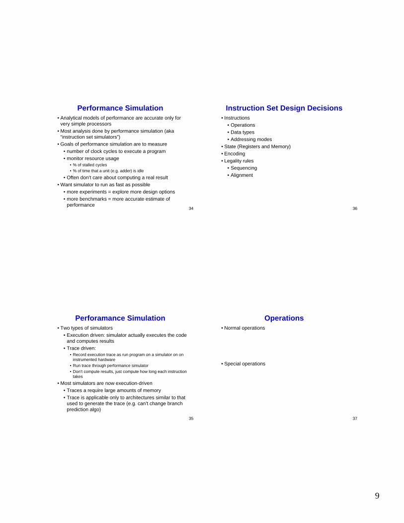
34
Performance Simulation• Analytical models of performance are accurate only for
very simple processors• Most analysis done by performance simulation (aka
“instruction set simulators”)• Goals of performance simulation are to measure
• number of clock cycles to execute a program• monitor resource usage
• % of stalled cycles• % of time that a unit (e.g. adder) is idle
• Often don’t care about computing a real result• Want simulator to run as fast as possible
• more experiments = explore more design options• more benchmarks = more accurate estimate of
performance
35
Perforamance Simulation• Two types of simulators
• Execution driven: simulator actually executes the code and computes results
• Trace driven: • Record execution trace as run program on a simulator on on
instrumented hardware• Run trace through performance simulator• Don’t compute results, just compute how long each instruction
takes
• Most simulators are now execution-driven• Traces a require large amounts of memory• Trace is applicable only to architectures similar to that
used to generate the trace (e.g. can’t change branch prediction algo)
36
Instruction Set Design Decisions• Instructions
• Operations• Data types• Addressing modes
• State (Registers and Memory)• Encoding• Legality rules
• Sequencing• Alignment
37
Operations• Normal operations
• Special operations
10
38
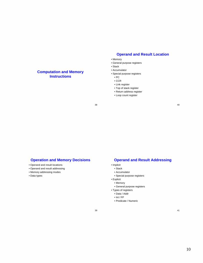
Computation and Memory Instructions
39
Operation and Memory Decisions• Operand and result locations• Operand and result addressing• Memory addressing modes• Data types
40
Operand and Result Location• Memory• General purpose registers• Stack• Accumulator• Special purpose registers
• PC• CCR• Link register• Top of stack register• Return address register• Loop count register
41
Operand and Result Addressing• Implicit
• Stack• Accumulator• Special purpose registers
• Explicit• Memory• General purpose registers
• Types of registers• Data / Addr• Int / FP• Predicate / Numeric

11
42
Memory Addressing• Alignment
• Byte, Half-word, Word, Double-word• Addressing modes
• Register• Immediate• Displacement• Register indirect• Indexed• Direct (or absolute)• Memory indirect• Pre/Post inc/dec rement• Scaled
43
Data Width• Most common data widths:
• 8b byte• 16b short• 32b word• 64b double
• Special cases• Internal registers of greater width to improve precision
of arithmetic• Vectors
• MMX vs general vector instructions
• CISC strings
44
Control Flow Instructions
45
Programming Language Control FlowProgramming language constructs that lead to
control flow instructions• Case/switch• If-then-else• Subroutine, procedure, function call• Subroutine, procedure, function return• Loop
12
46
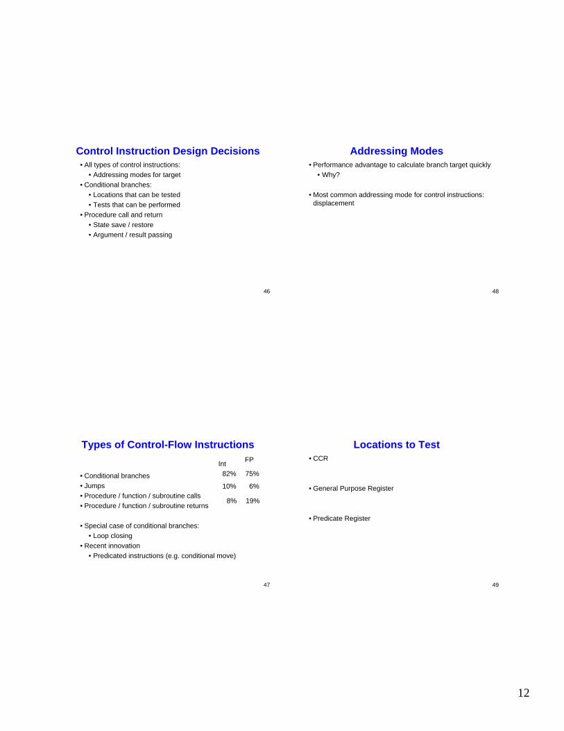
Control Instruction Design Decisions• All types of control instructions:
• Addressing modes for target• Conditional branches:
• Locations that can be tested• Tests that can be performed
• Procedure call and return• State save / restore• Argument / result passing
47
Types of Control-Flow Instructions
• Conditional branches• Jumps• Procedure / function / subroutine calls• Procedure / function / subroutine returns
• Special case of conditional branches:• Loop closing
• Recent innovation• Predicated instructions (e.g. conditional move)
8%
10%
82%
19%
6%
75%Int FP
48
Addressing Modes• Performance advantage to calculate branch target quickly
• Why?
• Most common addressing mode for control instructions: displacement
49
Locations to Test• CCR
• General Purpose Register
• Predicate Register

13
50
Tests• Flag set / unset• Comparison• <0, ≤0, =0, ≥0, >0
51
State Save/Restore• What’s the problem?
• In CISC processors, often could save or restore state with a single instruction.
• VAX Calls instruction: extremely general, extremely slow, not used.
• RISC approach: • let compiler do the work• establish compiler conventions
• caller-save or callee-save• registers for stack pointer and link pointer
• Register windows
52
Argument/Result Passing• Similar to state save/restore
• CISC: special purpose instructions• RISC: let the compiler do the work
• RISC alternative: register windows• Berkeley RISC I, SUN Sparc, Intel Itanium• Architectural carbunkle or elegant alternative to
register renaming?
53
Example: Braniac vs Speed Demon• AMD Athlon 1.2 GHz, 409 SPECint• Fujitsu SPARC64: 675 MHz, 443 SPECint• Assume that it requires 20% more instructions to write a
program in Sparc64 than in IA-32• Q: Which processor has higher performance?
• Q: What is the ratio between the CPIs?
• Q: What is the CPI of the AMD Athlon?
14
54
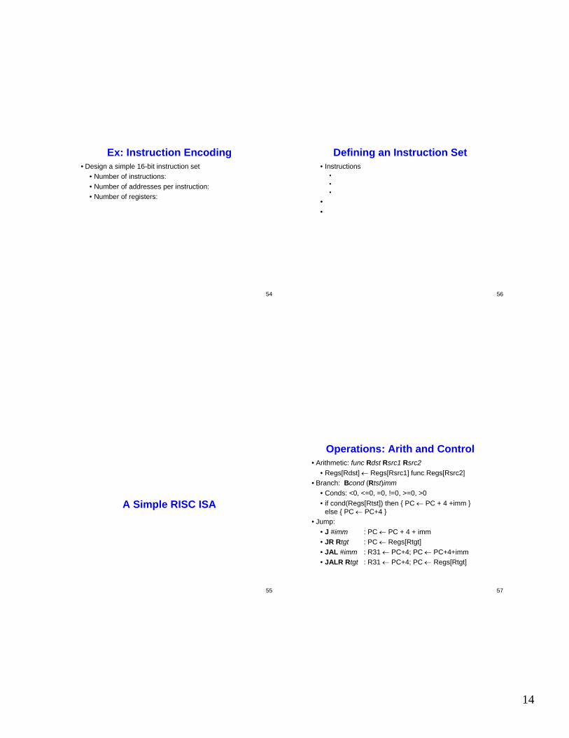
Ex: Instruction Encoding• Design a simple 16-bit instruction set
• Number of instructions:• Number of addresses per instruction:• Number of registers:
55
A Simple RISC ISA
56
Defining an Instruction Set• Instructions
•••
••
57
Operations: Arith and Control• Arithmetic: func Rdst Rsrc1 Rsrc2
• Regs[Rdst] ← Regs[Rsrc1] func Regs[Rsrc2]• Branch: Bcond (Rtst)imm
• Conds: <0, <=0, =0, !=0, >=0, >0• if cond(Regs[Rtst]) then { PC ← PC + 4 +imm }
else { PC ← PC+4 }• Jump:
• J #imm : PC ← PC + 4 + imm• JR Rtgt : PC ← Regs[Rtgt]• JAL #imm : R31 ← PC+4; PC ← PC+4+imm• JALR Rtgt : R31 ← PC+4; PC ← Regs[Rtgt]
15
58
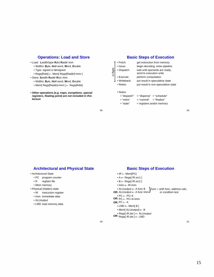
Operations: Load and Store• Load: Lwidth/type Rdst Raddr imm
• Widths: Byte, Half-word, Word, Double• Type: signed or Unsigned• Regs[Rdst] ← Mem[ Regs[Raddr]+imm ]
• Store: Swidth Raddr Rsrc imm• Widths: Byte, Half-word, Word, Double• Mem[ Regs[Raddr]+imm ] ← Regs[Rdst]
• Other operations (e.g. traps, exceptions, special registers, floating point) are not included in this lecture
59
Architectural and Physical State• Architectural State
• PC program counter• R register file• Mem memory
• Physical (hidden) state• IR instruction register• Imm immediate data• ALUoutput• LMD load memory data
60
Basic Steps of Execution• Fetch: get instruction from memory• Issue: begin decoding, enter pipeline• Dispatch: wait until operands are ready,
send to execution units• Execute: perform computation• Writeback: put result in speculative state• Retire: put result in non-speculative state
• Notes: • “dispatch” = “disperse” = “schedule”• “retire” = “commit” = “finalize”• “state” = registers and/or memory
in-fl
ight
61
Basic Steps of Execution• IR ← Mem[PC]• A ← Regs[ IR.src1 ]• B ← Regs[ IR.src2 ]• Imm ← IR.imm• ALUoutput ← A func B
ALUoutput ← A func Imm• PC ← PC+4
PC ← PC+4+immPC ← A
• LMD ← Mem[ B ]• Mem[ ALUoutput] ← B• Regs[ IR.dst ] ← ALUoutput
Regs[ IR.dst ] ← LMD
OR:
OR:
OR:
func = arith func, address calc, or condition test}
OR:

16
62
A Simple ProcessorMem
IRA
BALUoutput
Imm
LMD
Add
rD
ata
PC
4
Src1Src2
Add
rD
ata
Add
rD
ata
Regs
Dst
Add
rD
ata
Add
rD
ata
63
Perform an ALU Reg-Reg instrMem
IRA
BALUoutput
Imm
LMD
Add
rD
ata
PC
4
Src1Src2
Add
rD
ata
Add
rD
ata
Regs
Dst
Add
rD
ata
Add
rD
ata
64
Perform an ALU Reg-Imm instrMem
IRA
BALUoutput
Imm
LMD
Add
rD
ata
PC
4
Src1Src2
Add
rD
ata
Add
rD
ata
Regs
Dst
Add
rD
ata
Add
rD
ata
65
Perform a StoreMem
IRA
BALUoutput
Imm
LMD
Add
rD
ata
PC
4
Src1Src2
Add
rD
ata
Add
rD
ata
Regs
Dst
Add
rD
ata
Add
rD
ata
17
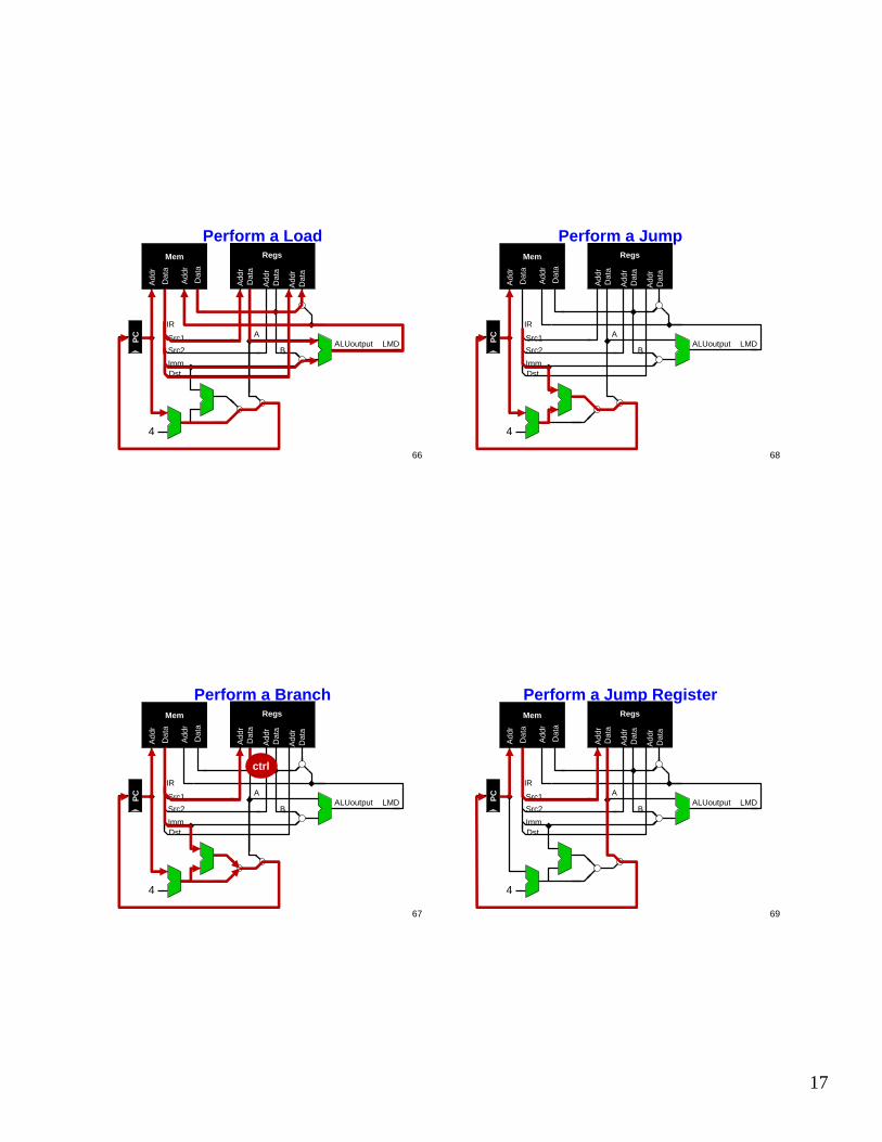
66
Perform a LoadMem
IRA
BALUoutput
Imm
LMD
Add
rD
ata
PC
4
Src1Src2
Add
rD
ata
Add
rD
ata
Regs
Dst
Add
rD
ata
Add
rD
ata
67
Perform a BranchMem
IRA
BALUoutput
Imm
LMD
Add
rD
ata
PC
4
Src1Src2
Add
rD
ata
Add
rD
ata
Regs
Dst
Add
rD
ata
Add
rD
ata
ctrl
68
Perform a JumpMem
IRA
BALUoutput
Imm
LMD
Add
rD
ata
PC
4
Src1Src2
Add
rD
ata
Add
rD
ata
Regs
Dst
Add
rD
ata
Add
rD
ata
69
Perform a Jump RegisterMem
IRA
BALUoutput
Imm
LMD
Add
rD
ata
PC
4
Src1Src2
Add
rD
ata
Add
rD
ata
Regs
Dst
Add
rD
ata
Add
rD
ata
18
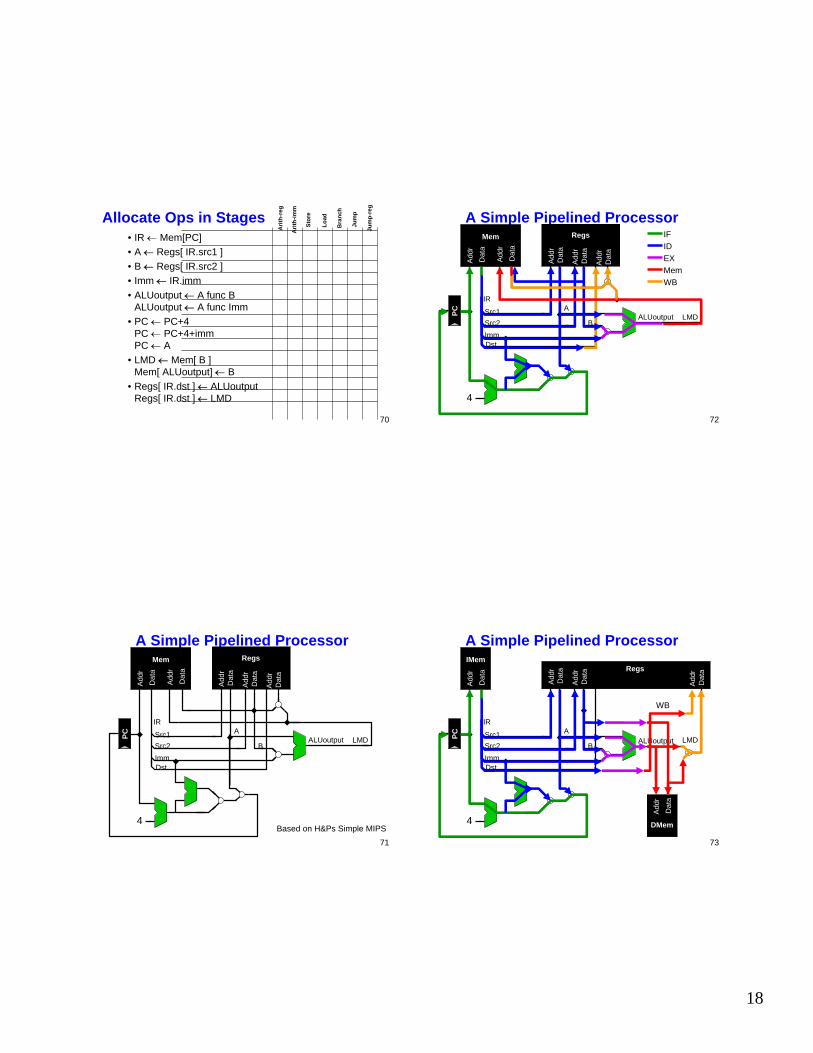
70
Allocate Ops in Stages• IR ← Mem[PC]• A ← Regs[ IR.src1 ]• B ← Regs[ IR.src2 ]• Imm ← IR.imm• ALUoutput ← A func B
ALUoutput ← A func Imm• PC ← PC+4
PC ← PC+4+immPC ← A
• LMD ← Mem[ B ]Mem[ ALUoutput] ← B
• Regs[ IR.dst ] ← ALUoutputRegs[ IR.dst ] ← LMD
Arit
h-re
g
Arit
h-im
m
Stor
e
Load
Bra
nch
Jum
p
Jum
p-re
g
71
A Simple Pipelined ProcessorMem
IRA
BALUoutput
Imm
LMD
Add
rD
ata
PC
4
Src1Src2
Add
rD
ata
Add
rD
ata
Regs
Dst
Add
rD
ata
Add
rD
ata
Based on H&Ps Simple MIPS
72
A Simple Pipelined ProcessorMem
IRA
BALUoutput
Imm
LMD
Add
rD
ata
PC
4
Src1Src2
Add
rD
ata
Add
rD
ata
Regs
Dst
Add
rD
ata
Add
rD
ata
IFIDEXMemWB
73
A Simple Pipelined ProcessorIMem
IRA
BALUoutput
Imm
LMD
Add
rD
ata
PC
4
Src1Src2
Add
rD
ata
Add
rD
ataRegs
Dst
Add
rD
ata
WB
DMem
Add
rD
ata
19
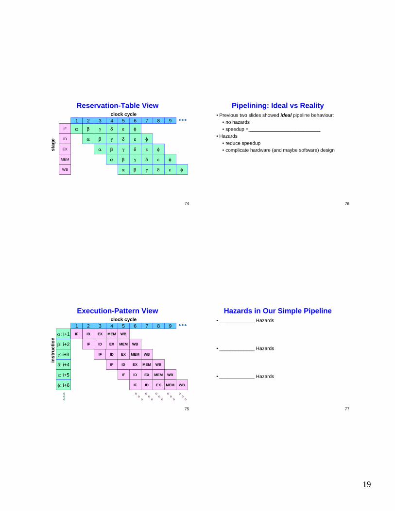
74
Reservation-Table Viewclock cycle
stag
e
1 2 3 4 5 6 7 8 9α β γ δIF
ID
EX
MEM
WB
α
α
α
α
β γ δ
β γ δ
β γ δ
β γ δ
ε φ
ε φ
ε φ
ε φ
ε φ
75
Execution-Pattern Viewclock cycle
inst
ruct
ion
1 2 3 4 5 6 7 8 9α: i+1
β: i+2
γ: i+3
δ: i+4
IF
IF
IF
IF
ID EX MEM WB
ID EX MEM WB
ID EX MEM WB
ID EX MEM WB
ε: i+5
φ: i+6
IF
IF
ID EX MEM WB
ID EX MEM WB
76
Pipelining: Ideal vs Reality• Previous two slides showed ideal pipeline behaviour:
• no hazards• speedup = __________________________
• Hazards • reduce speedup• complicate hardware (and maybe software) design
77
Hazards in Our Simple Pipeline• _____________ Hazards
• _____________ Hazards
• _____________ Hazards
20
78
clock cycle
stag
e
1 2 3 4 5 6 7 8 9IF
ID
EX
MEM
WB
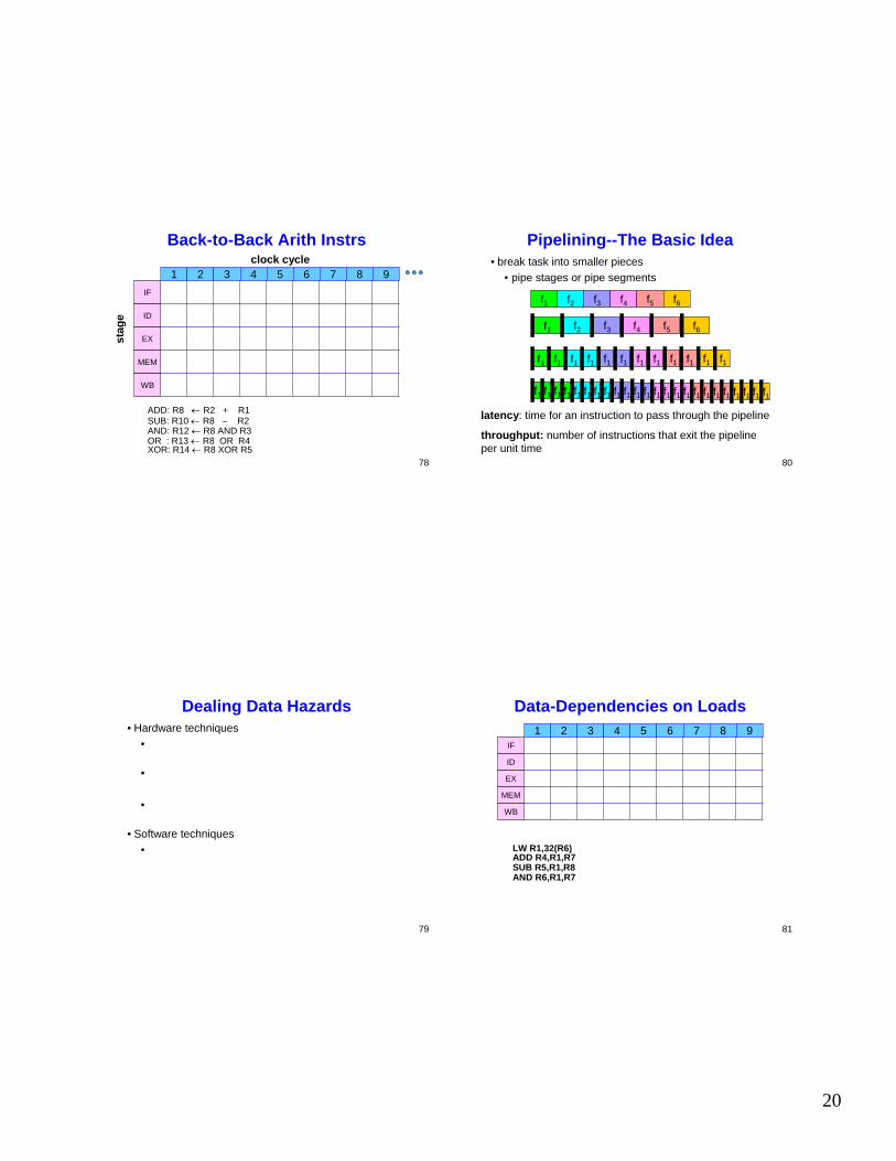
Back-to-Back Arith Instrs
ADD: R8 ← R2 + R1SUB: R10 ← R8 – R2AND: R12 ← R8 AND R3OR : R13 ← R8 OR R4XOR: R14 ← R8 XOR R5
79
Dealing Data Hazards• Hardware techniques
•
•
•
• Software techniques•
80
Pipelining--The Basic Idea• break task into smaller pieces
• pipe stages or pipe segments
latency: time for an instruction to pass through the pipeline
f1 f2 f3 f4 f5 f6
f1 f1 f1 f1 f1 f1 f1 f1 f1 f1 f1 f1
f1 f1 f1 f1 f1 f1 f1 f1 f1 f1 f1 f1 f1 f1 f1 f1 f1 f1 f1 f1 f1 f1 f1 f1
f1 f2 f3 f4 f5 f6
throughput: number of instructions that exit the pipeline per unit time
81
Data-Dependencies on Loads
AND R6,R1,R7SUB R5,R1,R8ADD R4,R1,R7LW R1,32(R6)
1 2 3 4 5 6 7 8 9
WB
MEM
EX
ID
IF
21
82
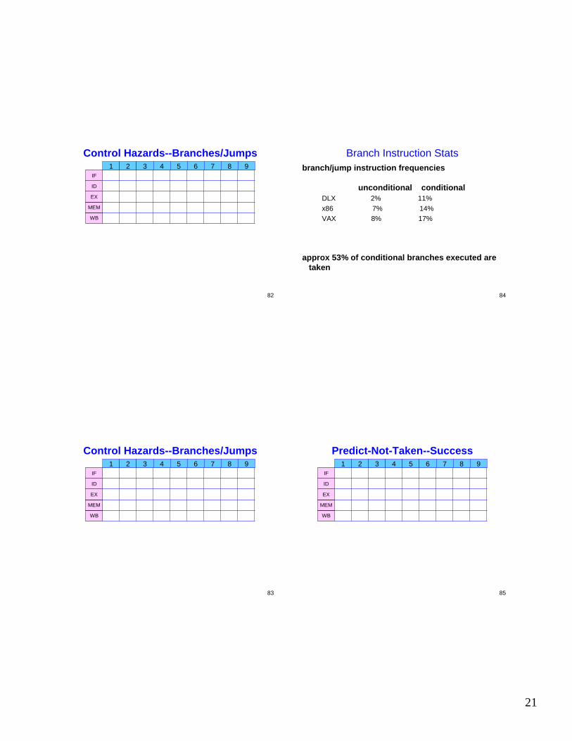
Control Hazards--Branches/Jumps1 2 3 4 5 6 7 8 9
WB
MEM
EX
ID
IF
83
Control Hazards--Branches/Jumps1 2 3 4 5 6 7 8 9
WB
MEM
EX
ID
IF
84
Branch Instruction Statsbranch/jump instruction frequencies
unconditional conditionalDLX 2% 11%x86 7% 14%VAX 8% 17%
approx 53% of conditional branches executed are taken
85
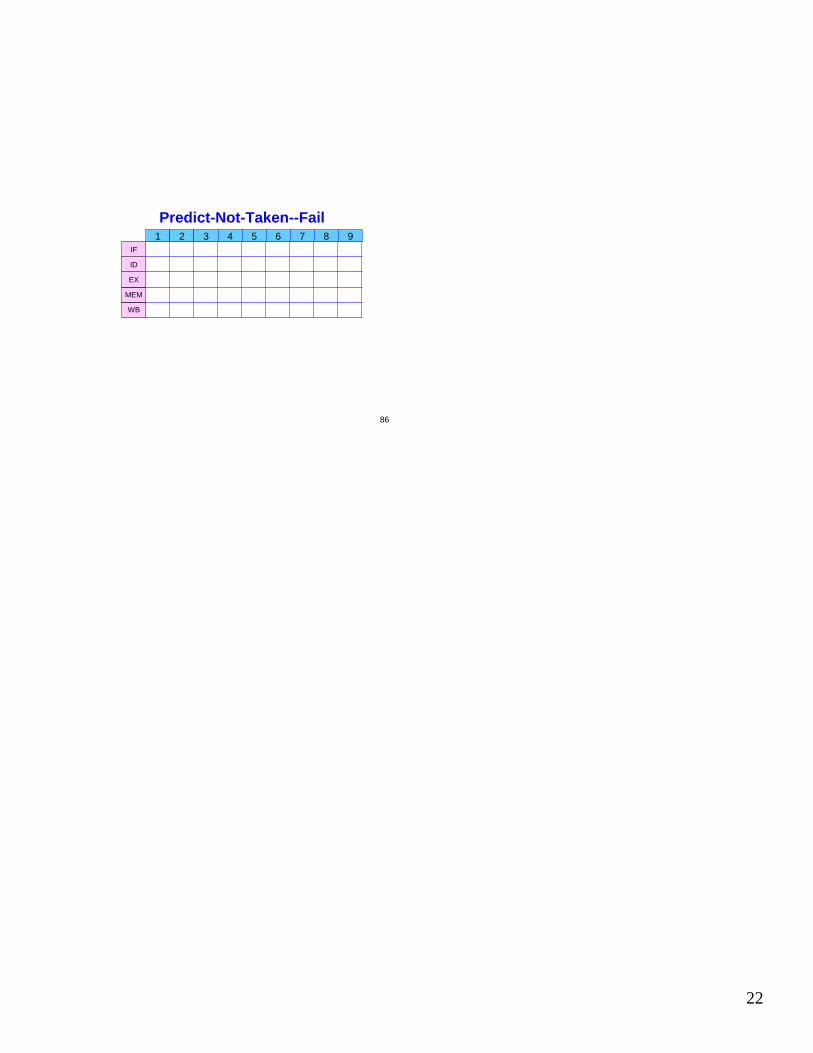
Predict-Not-Taken--Success1 2 3 4 5 6 7 8 9
WB
MEM
EX
ID
IF
22
86
Predict-Not-Taken--Fail1 2 3 4 5 6 7 8 9
WB
MEM
EX
ID
IF


