
5
Pathways for Quantitative Analysis by X-Ray Diffraction
J.D. Martín-Ramos1, J.L. Díaz-Hernández2, A. Cambeses1, J.H. Scarrow1 and A. López-Galindo3
1University of Granada, Department of Mineralogy and Petrology 2IFAPA Camino de Purchil, Departament of Natural Resources, Junta de Andalucía
3Instituto Andaluz de Ciencias de la Tierra (IACT, CSIC-UGR) Spain
1. Introduction
Quantitative analysis by powder X-Ray diffraction (Q-PXRD) is hardly ever carried out by
simple or obvious methods. Although the theory has been well established for some time
(Clark, 1936; Alexander et al., 1948; Chung, 1974, 1975; Brindley, 1980; Bish et al., 1988; etc.),
in practice imprecise results are obtained because of experimental oversimplification usually
introduced as a result of the complexity of the problem. Most of the usual methods are
based on the correspondence between the intensities diffracted by each crystalline phase
and their weight content in a multiple component mixture, without previously assuming
that this correspondence is linear.
A straightforward simplification of the general equation of the intensity diffracted by a crystal [1] allows us to estimate the weight fraction (Xp) of a phase (P) diffracting at intensity Ihkl,P[2]:
Ihkl,P = Io/64r · e2/mec2 Whkl/V2P · |Fhkl,P|2 · Lp· Xv,P /S (1)
(Whkl = multiplicity, V = unit-cell volume, Lp= Lorentz-polarization factor, Xv,P = volume fraction of phase P)
XP = KD · (/)S · (M · [C · I/|F|2]hkl )P (2)
In this expression, the subscripts refer to each phase (P) of the sample (S), to the experimental
geometry of the diffractometer (D) and to the reflections (hkl) of each of the individual phases.
This means that analysis quality is conditioned by factors affecting not only each component of
the sample analyzed, but also other factor including the set of minerals making up the sample
(/)S, texture (Chkl,P) and the experimental device itself KD, the last being a general constant
considered to be unvarying in all diffraction experiments in a given laboratory.
2. Methods of quantitative analysis
The various ways in which the parameters of formula [2] can be simplified give rise to the various methods of Q-PXRD.
www.intechopen.com

An Introduction to the Study of Mineralogy
74
2.1 Semi-quantitative or simple quantitative analysis
In this case, a single reflection is used per phase, absorption correction is omitted and the
result is adjusted so that the sum of XP = 1. The results obtained by this method usually have
considerable error and are not susceptible to statistical analysis. In other words:
XP = ([M · IDBmax/IDB· I]hkl )P (3)
with Mhkl,P being equivalent to 1/RIR, IDBmax = Maximum intensity of standard database
patterns (normally 100 or 1000) and IDB = Intensity of used reflection from database patterns.
When the maximum intensity reflection is used, the value of IDBmax/IDB is obviously 1.
The example shown in table 1 corresponds to a semi-quantitive analysis of the diffractogram
from figure 1 (sample F3). The scale factors are taken from database PDF2 (International
Centre for Diffraction Data, 2003), the reflections used were those with the highest
intensities and without interferences with other phases. Percentages are given as whole
numbers given that the maximum permitted precision is around 10%. The correct results are
those given in table 3 (see below) they differ significantly from the results in table 1.
Phase hkl Set-file Int(100) RIR %
Aragonite 111 41-1475 7.4 1.00 12
Calcite 104 81-2027 100.0 0.31 49
Celestine 121 89-7355 10.2 0.53 8
Dolomite 104 73-2324 50.0 0.40 31
Sum 100
Table 1. Simple quantitative analysis (semi-quantitative) of a four high crystallinity components sample. Reference intensity ratio (RIR) are from PDF2 database pattern I/Icor values.
Fig. 1. Diffractogram pattern of the mineral mixture indicated. Grey points=calculated pattern. Purple line=observed pattern. Green = Difference between observed and calculated diffractograms + 50 % elevation.
www.intechopen.com

Pathways for Quantitative Analysis by X-Ray Diffraction
75
In a general way, by adding a known amount of internal-standard to the sample we can substantially improve the results of the semi-quantitative method. There is an abundance of bibliographical references on this subject beginning with Chung (1974). Otherwise, simplification is achieved by using the relation between the mass coefficients of the total sample and of each component (Absorption-Diffraction method).
XP = (Ihkl,S / Ihkl,P) . (/)P / (/)S (4)
2.2 Rietveld methods
In this case the complete profile of the theoretical diffractogram that best fits the
experimental results is calculated on the basis of the known crystalline structures of the
sample components, the fit of some instrumental parameters, and the distribution functions
describe the shape of the reflections.
The method depends on the relationship:
WP = (S·M·V)P / (S·Z·M·V)i (5)
(W = weight fraction, P = each phase, n = number of phases, i = blank notation (1 to n), S = Scale factor, Z = Number of formulas per unit-cell, M = Molecular weight, V = unit-cell Volume).
As in other quantitive methods it is necessary to use adequate Reference Intensity Ratio
(RIR) to obtain the best results. Non-linear minimal squares methods are used that minimize
the accordance factor, R, whose most general form is:
R = [w |Io - Ic|]i / [w Io]i (6)
(i = each experimental point (blank, 1 to number of measured points), o = observed intensities,
c = calculated intensities, w = statistic weight). The quantitative results are obtained on the
basis of the scale factors used by each diffractogram partially determined by the experimental
conditions. This process refines: the unit cell, coordinates, factors of temperature and atomic
occupancies, profile parameters (mainly width and asymmetry), 2 displacements, preferred
orientation, background radiation parameters, extinction and microabsorption. The orientation
factors and scale factors of each phase are also refined. This method is elegant. The R values
achieved can be very low and the diffractograms of differences (Io-Ic)i are usually very flat (i is
each point of the diffractogram), although at times the quality of an analysis may be masked
by the complicated mathematical operations and the results can have an ‘excessively’
theoretical component. There are there are several excellent programs that use Rietveld
methods in general, and some have been specifically created for use in quantitative analysis
(Quanto). See http://www.ccp14.ac.uk/solution/rietveld_software/index.html. Typical
Rietveld analyses for sample F3 are shown in table 2 and in figure 2.
2.3 Full pattern fitting using experimental data
The relative mixtures of experimental diffractograms of pure phases can be used to simulate a problem sample using least squares methods (LS) as in the Rietveld method (Rietveld, 1969). If the chemical composition and the cell parameters of each phase are known,
www.intechopen.com

An Introduction to the Study of Mineralogy
76
Phase %
Aragonite 12.9 0.3
Calcite 53.9 0.3
Celestine 12.2 0.2
Dolomite 21.0 0.2
Table 2. Quantitative Rietveld analysis. Experimental data: 2θ step 0.01 º ; Radiation Cu K; Measured points= 5201; Counts per 8 sec; Total elapsed time = 702 min ; Maximum measured counts= 1247002 (divided by a suitable factor by set in appropriate scale); Final RInt = 0.0382.
Fig. 2. A) Rietveld plot showing experimental patterns (green), calculated pattern (grey points), difference pattern (red line at diffractogram middle maximum). B) Details of Rietveld analysis of sample F3, Bragg´s bar positions and their unique full-profiles. 2θ positions of partial components are displayed before zero shift refinement
absorption corrections can be made. This is a real alternative to the Rietveld methods that
can sometimes provide more realistic solutions. In general, we can omit the tuning of some
instrumental factors and other aspects concerning the sample itself that might affect the final
results, such as profile parameters, orientation parameters or radiation background. The
method behaves like a black-box model regarding the crystalline structure of each phase,
but this can only be an advantage when starting with phases with a chemical composition,
crystallinity and orientation model similar to those of the sample in question. This method is
www.intechopen.com

Pathways for Quantitative Analysis by X-Ray Diffraction
77
that of the XPowder© program, which uses a definition of the RInt parameter very similar to
the general one in equation [6].
RInt = { [ w ( Io-Ic )2 ]i / [w · Io2 ]i } (n· p) (7)
where Io are observed intensities and Ic calculated intensities, I = each experimental point, n = number of experimental points, p = number of standard patterns, (n· p) is constant for each analysis and is used only for scale purposes.
Another factor that has to be taken into account is the variation in absorption coefficients of each multiple component mixture and each component in isomorphic phases. A range of correction models have been used (for example see [4]), these usually produce different results that depend on the geometry of the diffractometer. The best result is usually obtained by using a multicomponent standard that has similar mass absorption coefficients to the analyzed sample. In this case the composition of each component is affected by a scale factor given by:
Si = [Xi/ Xp] · [W%p /W%i ] (8)
where i is each component; P is the reference component that should be the most common in the samples (although not necessarily present in all of them); X is the weight fraction of each component of the diffractogram, and W% is the real weight of each component in the matrix W (see Appendix [A6]). Of course, these factors only have to be calculated for the standard sample, formed of the components i and P. This approximation gives sufficiently exact results.
An additional advantage is that amorphous phases can be treated in the same way as the crystalline compounds, if the isolated amorphous component is available. When all the partial diffractograms and the given sample are recorded in the same experimental conditions (same sample carrier, recording conditions, etc.) and the intensity of the incident rays is stable, it is not usually necessary to carry out any scale correction when absolute units or time units are used. However, if the intensities are used in relative mode (e.g., when the values are adjusted to a maximum value of 1000) a standard sample of known composition must be used to calculate the MP factor of each phase.
This method also has the advantage that it is not necessary to perform the diffractogram analyses with the precision needed by the Rietveld method. As is well known the latter requires static analysis of various seconds per point (see 2.2, table 2), with between measurement intervals (2θ step) of 0.02 and 0.002º of 2θ. Analysis of a sample under such
conditions can take up to a whole day. With the method discussed in this section, it is enough to use the typical working method of any diffractometer laboratory (12 to 30 minutes per analysis) but making sure to analyze standards under the same conditions. On the other hand, with the current method it is not necessary to adjust the ‘instrumental function’, ‘Caglioti function’, asymmetry, sample profile function, etc., given that these data are included in the standard analyses. In any case, it is clear that the results are more correct when the quality of the experimental data is better.
The main difficulty for application of this method is finding suitable standard substances. However, they can be obtained and when available the results are very precise. Table 3 shows the data for XPowder© program quantitative batch mode analysis of various samples that have the same qualitative composition as before.
www.intechopen.com

An Introduction to the Study of Mineralogy
78
Sample Ara Ara- Cal Cal- Cel Cel- Dol Dol- Rint Cycles Sigma
F1 19.5 0.2 40.0 0.2 19.8 0.2 20.7 0.2 0.00499 3 0.00064 F2 15.6 0.2 33.6 0.2 32.8 0.2 18.0 0.3 0.00467 3 0.00060 F3 14.3 0.2 53.8 0.2 13.2 0.2 18.6 0.2 0.00369 3 0.00061 F4 27.6 0.3 21.5 0.4 41.0 0.3 10.0 0.5 0.00604 3 0.00068 F5 22.0 0.2 30.9 0.2 6.0 0.2 41.1 0.2 0.00439 2 0.00064
Table 3. Qualitative and quantitative composition of studied samples and standard deviation. Note that R values are <<0.01, indicating good adjustment. Known % weigh quantitative composition of sample F1 are: Ara: Aragonite 19.53, Cal: Calcite 39.91, Cel: Celestine 19.86 and Dol: Dolomite 20.71 was used as P component in [8]. With σ, as a standard deviation results of adjustment of each mineral.
In any case, there are multiple occasions when it is not necessary to evaluate the whole sample and so it is not necessary to have all the individual standards. The possibility to use natural or synthetic standards provides the opportunity to analyze individual components instead of a crystalline or partially amorphous matrix, always when a stable diffractogram is produced. As an example, it is possible to estimate the amount of a mineral in an organic matrix mix; the principal active pharmaceutical component amongst commercial additive such as starch or lactose; the amount of gypsum added to ‘clinker‘ powder in a ‘Portland‘ cement.
The given examples, and also the following, were obtained the XPowder© program that allows the component total to be adjusted to 100%, or alternatively to use one of the components, artificially added or not, as an internal standard with an aim to determine the absolute quantity of each independently of the composition of the components in the mix. The details of the calculation performed are in the appendix. The functions defined in the present work include adjustments of possible 2θ angle displacements, corrections related to component absorption coefficients as estimated from the database chemical formulas and absorption mass coefficient of the whole sample that is obtained iteratively from the calculated mineral composition. An option is that the intensity values can be statistically weighed with I-½.
The application of this method is simple in transformations that convert one crystalline phase into another during a natural industrial process. It is also useful in crystalline processes in which the independent variable is, for example, time, concentration, pressure or temperature. The method is very precise when the chemical composition varies bit by bit, such as in dehydration for example. Crystallization of adhesives has been successfully tested as has crystallization of cements and cement glues and sulphate dehydration of Mg, Ca and Na (Cardell et al., 2007).
The following example (figure 3) is of the dehydration transformation of hidrotalcite. The process was monitored by X-ray diffraction and the results represented on a bidimensional map where colours represent relative intensities (greys represent low intensities). Angles are shown on the x-axis and temperatures on the y-axis. Recrystallization began during heating at around 100ºC. In this example the absorption correction was not done because of lack of information about the samples true composition. Nevertheless, this correction should not be important given that few changes are noted in the global chemistry. For the quantitative calculation the first and last diffractograms were used as standards, the others were defined as a sample of these.
www.intechopen.com

Pathways for Quantitative Analysis by X-Ray Diffraction
79
Fig. 3. XPowder© false colour 2D representation that shows the evolution of the diffractograms of hidrotalcite obtained during heating between 25-150ºC. The image corresponds to the computer screen, so the characters are reduced to be able to read them in the present format: the header presents the database mineral information, in different colours and with diameters for each reflection point, including the hkl reflection. The false colour represents the relative intensities, absolute values are shown by contour lines.
Table 4 shows the low values obtained for RInt and standard deviation (. This indicates the
high quality of the results. These highest indices values correspond to temperatures between
95 and 115 ºC. This is due to the presence of an important amorphous phase produced
between the melting of the low temperature phase and the crystallization of the new high
temperature phase. These results could be improved with a longer diffractogram analysis
with a more gradual temperature increase. Diffractograms may also be used to 100 ºC to
quantify the process, such that an third amorphous low crystallinity component could easily
be evaluated.
The method that adjusts the whole profile permits weighting between components that have
an identical nature but somewhat different characteristics. For example, it is possible to use
standards with very different crystallinities to weight the crystallinities of minerals
intermediate compositions. This method has recently been used in very low crystallinity
such as starch in the food industry. Use of this peculiarity is common in classic
mineralogical studies about the measurement of illite, graphite, carbonates, etc. Despite this
www.intechopen.com

An Introduction to the Study of Mineralogy
80
it is common to weight the crystallinity using the classic method full width, half maximum
(FWHM) that is not very sensitive in most cases, or is affected by the diffractometer optics
especially by instrumental function which makes the analysis unreliable despite a frequent
use of phase standards.
Sample ºC Deh σ Hyd σ Rint cycles σ
HTC_001 25 0.0 0.0 100.0 0.0 0.00000 2 0.00000
HTC_002 30 1.7 0.6 98.3 0.5 0.00155 2 0.00005
HTC_003 35 1.5 0.6 98.5 0.5 0.00171 2 0.00006
HTC_004 40 1.7 0.6 98.3 0.5 0.00163 2 0.00005
HTC_005 45 1.8 0.6 98.2 0.5 0.00175 2 0.00006
HTC_006 50 3.1 0.7 96.9 0.5 0.00218 2 0.00006
HTC_007 55 3.7 0.7 96.3 0.6 0.00242 2 0.00007
HTC_008 60 4.8 0.8 95.2 0.6 0.00280 2 0.00007
HTC_009 65 6.6 0.9 93.4 0.7 0.00433 2 0.00009
HTC_010 70 8.6 0.9 91.4 0.8 0.00446 2 0.00009
HTC_011 75 12.4 1.0 87.6 0.9 0.00569 3 0.00010
HTC_012 80 15.2 1.1 84.8 1.0 0.00704 3 0.00012
HTC_013 85 21.3 1.4 78.7 1.2 0.00844 3 0.00013
HTC_014 90 25.9 1.5 74.1 1.4 0.00973 3 0.00014
HTC_015 95 33.3 1.8 66.7 1.6 0.01166 3 0.00016
HTC_016 100 41.2 1.8 58.8 1.7 0.01116 3 0.00016
HTC_017 105 50.0 2.1 50.0 2.1 0.01094 3 0.00016
HTC_018 110 59.2 1.8 40.8 1.8 0.00712 3 0.00013
HTC_019 115 67.5 1.5 32.5 1.6 0.00620 3 0.00012
HTC_020 120 74.6 1.1 25.4 1.1 0.00416 3 0.00010
HTC_021 135 79.9 0.8 20.1 0.9 0.00333 3 0.00009
HTC_022 140 85.1 0.7 14.9 0.8 0.00278 2 0.00008
HTC_023 145 90.9 0.6 9.1 0.7 0.00257 2 0.00008
HTC_024 150 95.3 0.5 4.7 0.6 0.00199 2 0.00006
HTC_025 155 97.3 0.5 2.7 0.6 0.00191 2 0.00006
HTC_026 160 100.0 0.0 0.0 0.0 0.00000 2 0.00000
Table 4. XPowder© output quantitative analysis in a thermodiffraction analyses of hidrotalcite. Sum fitted 100 %. The percentages have been calculated weighing data. Angles 2θ have been refined. Normalization criteria: Max. counts = 1.
The possibility to break a diffractogram down into its component parts (figure 4) permits consideration of additional aspects in the interpretation of results. So, some ideas, such as the profile studies (for example Williamson-Hall, 1953 or Warren-Averbach, 1950) require availability of diffractograms of pure phases. In the example of figure 5, difference diagram mainly correspond to dolomitic phase diagram.
www.intechopen.com

Pathways for Quantitative Analysis by X-Ray Diffraction
81
Fig. 4. Detail of the analysis represented in figure 1 that also includes the partially weighted components obtained in the least-squares calculation.
Fig. 5. Isolation of one of the components from the whole diffractogram. In the example the graph of differences coincides with the isolated diffractogram of dolomite, given that this was not included in the calculation and so was the main cause of the differences between the observed and calculated graphics.
3. Adjustement of diffractogram to bar-chart database content
This method can be used when pure phases of sample components are not available, It
consists in adjusting the theoretical mixture of the bar-charts found in some databases
(PDF2, AMCSD, etc.) to the sample diffractogram. The proportion of each component used
in this mixture forms the basis for the quantitative calculation. This method is also contained
in the XPowder© program, which uses non-linear least-squares methods for the calculation
and definition of Rint of [6]. The 2 database content and experimental diagram values can
be redefined (see figure 6, table 5).
www.intechopen.com
An Introduction to the Study of Mineralogy
82
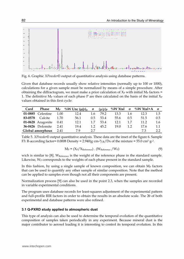
Fig. 6. Graphic XPowder© output of quantitative analysis using database patterns.
Given that database records usually show relative intensities (normally up to 100 or 1000), calculations for a given sample must be normalized by means of a simple procedure. After obtaining the diffractogram, we must make a prior calculation of XP with initial MP factors = 1. The definitive MP values of each phase P are then calculated on the basis of the initial XP values obtained in this first cycle:
Card Phase MP %W Unc (µ/)p σ P %W Xtal σ %W Xtal+A σ
01-0885 Celestine 1.00 12.4 1.6 79.2 13.3 1.6 12.3 1.5 83-0578 Calcite 1.70 56.1 0.5 53.4 55.6 0.5 51.5 0.5 01-0628 Aragonite 0.41 12.1 1.7 53.4 12.1 1.7 11.2 1.6 36-0426 Dolomite 2.41 19.4 1.2 45.2 19.0 1.2 17.6 1.1 Global amorphous 2.41 7.9 2.7 7.3 2.2
Table 5. XPowder© output quantitative analysis. These data are the inset of the figure 6. Sample F3: R-according factor= 0.0008 Density = 2.940(g·cm-³) µ/Dx of the mixture = 55.0 cm²·g-¹.
MP = (XP/XReference) . (WReference /WP) (9)
wich is similar to [8]. WReference is the weight of the reference phase in the standard sample. Likewise, WP corresponds to the weights of each phase present in the standard sample.
In this fashion, by using a single sample of known composition, we can obtain MP factors that can be used to quantify any other sample of similar composition. Note that the method can be applied to samples even though not all their components are present.
Normalization process [9] can also be used in the point 2.3, when the samples are recorded in variable experimental conditions.
The program uses database records for least-squares adjustment of the experimental pattern and full-profile RIR factors in order to obtain the results in an absolute scale. The 2 of both experimental and database patterns were also refined.
3.1 Q-PXRD study applied to atmospheric dust
This type of analysis can also be used to determine the temporal evolution of the quantitative composition of samples taken periodically in any experiment. Because mineral dust is the major contributor to aerosol loading it is interesting to control its temporal evolution. In this
www.intechopen.com

Pathways for Quantitative Analysis by X-Ray Diffraction
83
way it has been possible to study atmospheric dust and its temporal evolution (figure 7 and table 6) in the south of the Iberian peninsula as is shown in the following example.
The standard patterns for individual phases were obtained to pure minerals belonging mainly from the Mineralogy Museum, University of Granada, forming thus a database of pure standard phases with initial ‘Scale Factors’ = 1. The RIR values for the complete profiles were calculated using [9]. The know composition of same samples was used as a standard. In addition, quartz was a common standard for all samples. The goodness of the fit was assessed using the according factor (RInt) for quantification obtained by the XPowder© program using the expression [7], with n=p=1.
RInt > 0.1 imply represent good analyses. On the contrary, RInt imply rejection of the analysis and the factors involved in this error must be studied (generally due to experimental causes). In the case of persistent error, the pattern must be rejected.
Fig. 7. XPowder© false colour 2D representation of the temporal evolution of mineral phases contained on atmospheric dust deposited on south-eastern Spain along 1992. Note the continuity of quartz during the sampling period.
In this example the following mineral phases have been detected (table 6): bassanite, calcite, chlorite, dolomite, feldspars, graphite, gypsum, halite, kaolinite, illite/muscovite, paragonite, quartz and various smectite types. In addition, some non-classifiable amorphous materials were quantified. From these results interesting conclusions can be draw about the behaviour of mineral aerosols in the atmosphere and enviroment (Díaz-Hernández et al., 2011), as for example the role played by smectites in the atmospheric processing of SO2 and in secondary sulphate genesis.
www.intechopen.com

An Introduction to the Study of Mineralogy
84
Table 6. XPowder© output quantitative analysis of samples of figure 7. Qtz: Quartz; Fd: Feldespar; Gph: Graphite; Cal: Calcite; Dolo: Dolomite; Bas: Bassanite; Gyp: Gypsum; Hal: Halite; Sm: Smectite; Clh: Clinochlore; Mus: Muscovite; Par: Paragonite; Kao: Kaolinite; A: Amorphous and R: according factor.
www.intechopen.com

Pathways for Quantitative Analysis by X-Ray Diffraction
85
3.2 Q-PXRD study applied to potassic volcanic rocks
Volcanic rocks are excellent samples to apply Q-PXRD study because in many cases mineral
grain size is very fine and it is difficult establish the modal proportions of minerals that
compose the rock, even if study is made using petrographic microscopy. Generally, potassic
volcanic rocks have a fine grain size related to fast cooling, among others factors (Mitchell
and Bergman, 1991). In these rocks it is necessary know the minerals that form the rock as
well as the modal proportions, which are one criteria to classify the sample in the potassic
volcanic rocks clan ( Mitchell and Bergman, 1991; Le Maitre et al., 2002).
Here we present the result of a Q-PXRDv study of the Zeneta potassic volcanic rocks of the
southeast of Spain volcanic region (Fig. 8), classified by many authors as lamproites
(Venturelli et al., 1984; Mitchell and Bergman, 1991; Toscani et al., 1995; Duggen et al., 2005;
Coticelli et al., 2009). However, recent studies show significant greats mineralogical and
geochemical variations, which indicate that the Zeneta volcanic rocks do not correspond to a
classical definition of lamproites (Cambeses, 2011).
Fig. 8. XPowder© false colour 2D representation of principal mineral phases showing in the most representative samples from rocks of Zeneta volcanic rocks.
Minerals identified in the Zeneta volcanic rocks in the XRD pattern and in petrographic thin section were olivine, diopside, biotite-phlogopite (brown mica), anorthite, sanidine and secondary quartz (Fig. 8). Quantification methodology was performed in fifty-six samples.
www.intechopen.com

An Introduction to the Study of Mineralogy
86
Table 7 includes representative analyses. The methodology is based on conversion to absolute values using scale factors for normalization as determined from the diffractogram of a standard with a know composition and modal proportion (sample Z_1_002 in Table 7). The mineral reference was sanidine, for the Zeneta volcanic rocks, due to its high crystallochemical stability its presence in all analyzed samples. The scale factor reference intensity ratios (RIR) were obtained from expression [9]. The goodness of the fit was assesed using the according factor (RInt) for quantification obtained using the XPowder© program from the expression [6], using n=p=1.
The results obtained show a very good correlation between Q-PXRD and petrographically determined modal proportions. For this reason we suggest that the XRD results for all samples indicate real petrographic modal proportions (Cambeses, 2011).
Knowing the mineral content of each of the samples permits determination of mineral distribution in the volcanic centre using a simple Krigin interpolation by creating layers with the same isovalues of mineral content based on the quantitative XRD results for each sample.
In Zeneta samples were selected distributed throughout the outcrop (Fig. 9A) and maps were made of all mineral phases identified in the fifty-six quantitative XRD analysis. In present work we show mapping of brown mica, diopside and sanidine distribution (Fig. 9B, C and D).
Fig. 9. A) Mapping from Zeneta volcanic rocks outcrop (Cambeses and Scarrow, submitted) B), C) and D) Q-PXRD data interpolated show Brown mica, diopside and sanidine relative modal proportion respectively.
www.intechopen.com

Pathways for Quantitative Analysis by X-Ray Diffraction
87
Table 7. Q-PXRD result from Zeneta volcanic rocks of olivine, Ol, diopside, Did, Phlogopite-biotite, Brw-M, Anorthite, An, Sanidine, San, Quartz, Qtz and amorphous, Amor. With σ, as a standard deviation results of adjustment of each mineral. R values is according factor related to adjustment in function of standard diffractogram. Coordinates in UTM projection.
www.intechopen.com

An Introduction to the Study of Mineralogy
88
Q-PXRD analyses indicate a heterogeneous distribution of minerals in the Zeneta volcanic rocks. Data obtained reveal how minerals such as diopside and sanidine, typical of lamproites (Mitchell and Bergman, 1991), have their highest modal proportions in central part of the outcrop (Fig. 9C and D). On other hand, brown micas have a higher modal proportion at the edge of the outcrop. Thus a process causing the mineralogical variation may be related to a petrogenetic model for the formation and emplacement of the potassic volcanic rocks (Cambeses, 2011).
For these reasons Q-PXRD analyses may be considered an excellent methodology for the study of volcanic and igneous rocks generally because it is a quick and simple method that provides valuable information about the modal proportions of all the mineral phases present in a sample. Results obtained are in good agreement with conventional methodologies such as modal proportion estimates from petrographic studies. In addition, Q-PXRD results indicate variations in mineral distributions throughout the outcrop potentially providing key information that can be used in petrogenetic interpretations.
4. Conclusions
The use of powerful computers with appropriate software facilitates X-Ray powder diffraction quantitative analysis. Nevertheless, the scientific literature only shows the use of massive semiquantitative analysis in which real measurements of reflective powers are not available because, in part, of the lack of natural standards that are pure enough and have a comparable crystallinity to the samples being studies. In the cases of precise analyses, obtaining good data requires an excessive amount of time in, for example, calculations. In this sense the Rietveld method was a great advance in controlling the experimental parameters and compositions and details of each mineral in mixes. Despite this, the productive capacity of this method is limited and requires a lot of data processing and data interpretation skills. In addition, even with excellent results complications in data processing may obscure data quality.
The least-squares method, applied to the calculation of a diffractogram that is to be compared with experimental data can be simplified as suggested by Rietveld if it is used to calculate experimental diffractograms from a database of a laboratory that applies these methods. This is what was done using methods 2.3 and 3 of the present chapter. Moreover, if pure standards are not available a complex known composition standard may be used to calculate global reference factors (full profile RIR) that can be applied to samples with a similar qualitative composition. Given that programs are available to do these calculations automatically it is possible to do these analyses in a routine manner on natural and industrial substances (online control in industry or mining). Table 8 shows the analytical results for sample F3, this allows the four methods to be compared.
The easiest to use method is ‘Simple Quantitative’ (semi-quantitative analysis), but this
includes large errors although the experimental work and calculations are simple. The
Rietveld method gives good results with small standard deviations but a considerable
amount of time and effort is required to obtain the results (analytical time 11.7 hours). This
necessitates selection of a preferential orientation model and refinement of paramenters
which could affect the calculation of the global scale factor for phases with few reflections.
The method is not applicable when the structure of some of the sample components is
www.intechopen.com
Pathways for Quantitative Analysis by X-Ray Diffraction
89
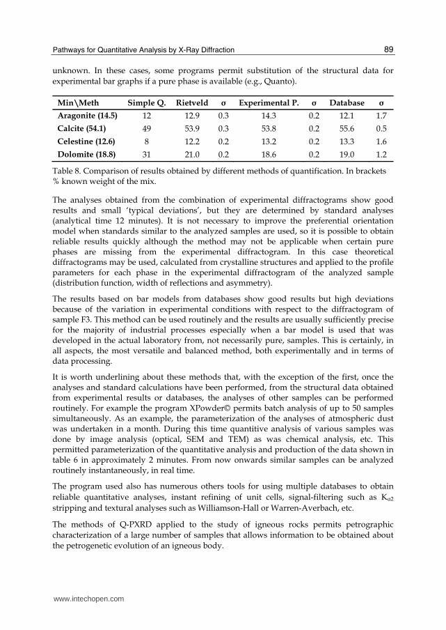
unknown. In these cases, some programs permit substitution of the structural data for
experimental bar graphs if a pure phase is available (e.g., Quanto).
Min\Meth Simple Q. Rietveld σ Experimental P. σ Database σ
Aragonite (14.5) 12 12.9 0.3 14.3 0.2 12.1 1.7
Calcite (54.1) 49 53.9 0.3 53.8 0.2 55.6 0.5
Celestine (12.6) 8 12.2 0.2 13.2 0.2 13.3 1.6
Dolomite (18.8) 31 21.0 0.2 18.6 0.2 19.0 1.2
Table 8. Comparison of results obtained by different methods of quantification. In brackets % known weight of the mix.
The analyses obtained from the combination of experimental diffractograms show good results and small ‘typical deviations’, but they are determined by standard analyses (analytical time 12 minutes). It is not necessary to improve the preferential orientation model when standards similar to the analyzed samples are used, so it is possible to obtain reliable results quickly although the method may not be applicable when certain pure phases are missing from the experimental diffractogram. In this case theoretical diffractograms may be used, calculated from crystalline structures and applied to the profile parameters for each phase in the experimental diffractogram of the analyzed sample (distribution function, width of reflections and asymmetry).
The results based on bar models from databases show good results but high deviations because of the variation in experimental conditions with respect to the diffractogram of sample F3. This method can be used routinely and the results are usually sufficiently precise for the majority of industrial processes especially when a bar model is used that was developed in the actual laboratory from, not necessarily pure, samples. This is certainly, in all aspects, the most versatile and balanced method, both experimentally and in terms of data processing.
It is worth underlining about these methods that, with the exception of the first, once the analyses and standard calculations have been performed, from the structural data obtained from experimental results or databases, the analyses of other samples can be performed routinely. For example the program XPowder© permits batch analysis of up to 50 samples simultaneously. As an example, the parameterization of the analyses of atmospheric dust was undertaken in a month. During this time quantitive analysis of various samples was done by image analysis (optical, SEM and TEM) as was chemical analysis, etc. This permitted parameterization of the quantitative analysis and production of the data shown in table 6 in approximately 2 minutes. From now onwards similar samples can be analyzed routinely instantaneously, in real time.
The program used also has numerous others tools for using multiple databases to obtain
reliable quantitative analyses, instant refining of unit cells, signal-filtering such as Kα2
stripping and textural analyses such as Williamson-Hall or Warren-Averbach, etc.
The methods of Q-PXRD applied to the study of igneous rocks permits petrographic
characterization of a large number of samples that allows information to be obtained about
the petrogenetic evolution of an igneous body.
www.intechopen.com

An Introduction to the Study of Mineralogy
90
5. Acknowledgments
This study was supported by the spanish projects CGL2010-16369, CGL2009-09249 and
CGL2008-02864 of the Ministerio de Ciencia e Innovación (MICINN), and by the Andalusian
grant RNM1595.
6. APPENDIX. The general least-squares methods used by the XPowder© program
Consideration on m linear functions (Y1 to Ym) with n variables. These variables can be
thought of as defining a space whose value at any point is determined by x1...xn and the
parameters w1…wn. If the values of the Y functions are measured at n different points (n
points for diffraction pattern), we can write:
w1X1,1+w2X1,2+...+wnX1,n = Y1 (being n>m) (A1)
w2X2,1+w2X2,2+...+wnX2,n = Y2
wmXm,1+w2Xm,2+...+wnXm,n = Ym
The principle of least squares (LS) states that the best values for parameters w1…wn are
those that minimize the sums of the squares of the differences between the experimental
(Yoi) and calculated (Yi) values of the function for all the observed (i) points.
Thus, the value to be minimized will be:
d = ∑i ωi (Yoi-Yi)2 with ωi = statistic weight, 1 ≤ i ≤ m (A2)
The minimization problem is treated by differentiating the right-hand side of [A2] in turn
and setting the derivative equal to zero:
∑i wi (Yoi-Yi) ∂Yi/∂wk = 0 with 1 ≤ k ≤ n (A3)
Expanding and rearranging:
∑iωiw1Xi,1Xi,1+ ∑iωiw2Xi,1 Xi,2 ··· + ∑iωiwm Xi,1 Xi,m = ∑iωiYoi Xi,1(A4)
∑iωiw1Xi,2Xi,1+ ∑iωiw2Xi,2 Xi,2 ··· + ∑iωiwm Xi,2 Xi,m = ∑iωiYoi Xi,2
∑iωiw1Xi,mXi,1+ ∑iωiw2Xi,m Xi,2 ··· + ∑iωiwm Xi,n Xi,n = ∑iωiYoi Xi,m
Solution of these m equations gives the best values of w parameters in the least-squares
sense.
In a matritial way:
X· W = Y (A5)
Where the elements of matrix X are defined as:
xf,c=∑iwiXi,f · Xi,c
www.intechopen.com

Pathways for Quantitative Analysis by X-Ray Diffraction
91
The elements of matrix Y are: yf= ∑i wiYoi Xi,f, where
i = 1, 2,… n (pattern points) f = 1, 2,… m (files) c = 1, 2,… m (columns)
X is a square symmetric matrix of know dimensions (m· m), W is a column matrix of unknowns, of dimension m, and Y is a know column matrix of dimension m. Multiplying each side of equation [A5] by X-1 gives:
X-1· X· W = X-1· Y
W = X-1· Y (A6)
with the W column being matrix the solution of a normal equation containing wi phase weights.
7. References
Alexander, L. & Klug, H.P. (1948). X-Ray diffraction analysis of crystalline dusts. Analitycal
Chemistry, Vol.20, No.10, pp. 886-894, ISSN 0003-2700.
Bish, D.L. & Howard, S.A. (1988). Quantitative phase analysis using the Rietveld method.
Journal of Applied Crystallography, Vol.21, No.2, pp. 86-91, ISSN 0021-8898.
Brindley, G.W. (1980). Quantitative X-Ray mineral analysis of clays. In G.W. Brindley and G.
Broen, eds. Crystal Structures of Clay Minerals and their X-Ray identification.
Mineralogical Society, London, pp. 411-438.
Cambeses, A. & Scarrow, J.H. (submitted). The Mediterranean Tortonian ‘salinity crisis’,
southern Spain: Potassic volcanic centres as potential paleographical indicators.
Geologica Acta, ISSN-1695-6133.
Cambeses, A. (2011). Caracterization of the volcanic centres at Zeneta and La Aljorra, Murcia:
evidence of minette formation by lamproite-trachyte magma mixing. Master thesis,
University of Granada, 249 pp.
Cardell, C.; Sánchez-Navas, A.; Olmo-Reyes, F.J. & Martín-Ramos, J.D. (2007). Powder X-
Ray thermodiffraction study of mirabilite and epsomite dehydration. Effects of
direct IR-irradiation on samples. Analitical Chemistry, Vol.79, No.12, pp. 4455-62,
ISSN 0003-2700.
Chung, F.H. (1974). Quantitative interpretation of X-Ray diffraction patterns of mixtures. I.
Matrix-flushing method of quantitative multicomponent analysis. Journal of Applied
Crystallography, Vol.7, No.6, pp. 519-525, ISSN 0021-8898.
Chung, F.H. (1975). Quantitative interpretation of X-Ray diffraction patterns. III.
Simultaneous determination of a set of reference intensities. Journal of Applied
Crystallography, Vol.8, No.1, pp. 17-19, ISSN 0021-8898.
Clark, G.L. & Reynolds, D.H. (1936). Quantitative analysis of mine dusts: an X-Ray
diffraction method. Industrial Engineering Chemistry, Analytical Edition, Vol.8, No.1,
pp. 36-40, ISSN 0096-4484.
Conticelli, S.; Guarnieri, L.; Farinelli, A.; Mattei, M.; Avanzinelli, R.; Bianchini, G.; Boari, E.;
Tommasini, S.; Tiepolo, M.; Prelevic, D. & Venturelli, G. (2009). Trace elements and
www.intechopen.com

An Introduction to the Study of Mineralogy
92
Sr-Nd-Pb isotopes of K-rich, shoshonitic, and calc-alkaline magmatism of the
Western Mediterranean Region: Genesis of ultrapotassic to calc-alkaline magmatic
associations in a post-collisional geodynamic setting. Lithos, Vol.107, pp. 68-92,
ISSN 0024-4937.
Díaz-Hernández, J.L.; Martín-Ramos, J.D. & López-Galindo, A. (2011). Quantitative
analysis of mineral phases in atmospheric dust deposited in the south-eastern
Iberian Peninsula. Atmospheric Environment, Vol.45, No.18, pp. 3015-3024, ISSN
1352-2310.
Duggen, S.; Hoernle, K.; Van Den Bogaard, P. & Garbe-Schonberg, D. (2005). Post-
Collisional Transition from Subduction- to Intraplate-type Magmatism in the
Westernmost Mediterranean: Evidence for Continental-Edge Delamination of
Subcontinental Lithosphere. Jounal of Petrology, Vol.46, No.16, pp. 1155-1201, ISSN
1460-2415.
Le Maitre, R. W.; Streckeisen, A.; Zanettin, B.; Le Bas, M.J.; Bonin, B. & Bateman, P. (Eds.).
(2002). Igneous Rocks. A Classification and Glossary of Terms. Recommendations of the
International Union of Geological Sciences Subcommission on the Systematics of Igneous
Rocks. Cambridge University Press, ISBN 0-521-66215-X, Cambridge.
Martín-Ramos, J.D. (2004). Using XPowder©, a software package for powder X-Ray
diffraction analysis. D.L.GR-1001/04. Spain. ISBN: 84-609-1497-6.
Mitchell, R. & Bergman, S.C. (Eds.). (1991). Petrology of Lamproites. Plenum Pres, ISBN 0-306-
43556-X, New York
Rietveld, H.M. (1969). A profile refinement method for nuclear and magnetic structures.
Journal of Applied Crystallography, Vol.2, No.2, pp. 65-71. ISSN 0021-8898.
Toscani, L.; Contini, S. & Ferrarini, M. (1995). Lamproitic rocks from Cabezo Negro de
Zeneta: Brown micas as a record of magma mixing. Mineralogy and Petrology,
Vol.55, No.4, pp. 281-292, ISSN: 1438-1168.
Venturelli, G.; Capedri, S.; Di Battistini, G.; Crawford, A.; Kogarko, L.N. & Celestini, S.
(1984). The ultrapotassic rocks from southeastern Spain. Lithos, Vol.17, pp. 37-54,
ISSN 0024-4937.
Warren, B.E. & Averbach, B.L. (1950). The effect of cold-work distortion on X-Ray patterns.
Journal of Applied Physics, Vol.21, No.6, pp. 595-599, ISSN 0021-8979.
Williamson, G.K. & Hall, W.H. (1953). X-Ray line broadening from filed aluminium and
wolfram. Acta Metallurgica, Vol.1, No.1, pp. 22-31, ISSN 0001-6160.
www.intechopen.com

An Introduction to the Study of MineralogyEdited by Prof. Cumhur Aydinalp
ISBN 978-953-307-896-0Hard cover, 154 pagesPublisher InTechPublished online 01, February, 2012Published in print edition February, 2012
InTech EuropeUniversity Campus STeP Ri Slavka Krautzeka 83/A 51000 Rijeka, Croatia Phone: +385 (51) 770 447 Fax: +385 (51) 686 166www.intechopen.com
InTech ChinaUnit 405, Office Block, Hotel Equatorial Shanghai No.65, Yan An Road (West), Shanghai, 200040, China
Phone: +86-21-62489820 Fax: +86-21-62489821
An Introduction to the Study of Mineralogy is a collection of papers that can be easily understood by a widevariety of readers, whether they wish to use it in their work, or simply to extend their knowledge. It is unique inthat it presents a broad view of the mineralogy field. The book is intended for chemists, physicists, engineers,and the students of geology, geophysics, and soil science, but it will also be invaluable to the more advancedstudents of mineralogy who are looking for a concise revision guide.
How to referenceIn order to correctly reference this scholarly work, feel free to copy and paste the following:
J.D. Martín-Ramos, J.L. Díaz-Hernández, A. Cambeses, J.H. Scarrow and A. López-Galindo (2012). Pathwaysfor Quantitative Analysis by X-Ray Diffraction, An Introduction to the Study of Mineralogy, Prof. CumhurAydinalp (Ed.), ISBN: 978-953-307-896-0, InTech, Available from: http://www.intechopen.com/books/an-introduction-to-the-study-of-mineralogy/pathways-for-quantitative-analysis-by-x-ray-diffraction


