
Paradise Lost and Found? The Econometric Contributions of Clive W.J. Granger and Robert F. Engle
by
Peter Hans Matthew
September 2004
MIDDLEBURY COLLEGE ECONOMICS DISCUSSION PAPER NO. 04-16
DEPARTMENT OF ECONOMICS MIDDLEBURY COLLEGE
MIDDLEBURY, VERMONT 05753
http://www.middlebury.edu/~econ
Paradise Lost and Found? The EconometricContributions of Clive W. J. Granger and
Robert F. Engle
Peter Hans MatthewsDepartment of Economics
Munroe HallMiddlebury College
Middlebury Vermont [email protected]
September 12, 2004
Abstract
This paper provides a non-technical and illustrated introduction tothe econometric contributions of the 2003 Nobel Prize winners, RobertEngle and Clive Granger, with special emphasis on their implications forheterodox economists.
Keywords: ARCH, GARCH, cointegration, error correction model,general-to-speci…c
JEL Codes: B23, B40, C22
1
1 Introduction1
The 2003 Bank of Sweden Nobel Prize in Economic Science was awarded to
Clive W. J. Granger, Professor Emeritus of Economics at the University of
California at San Diego, and Robert F. Engle, the Michael Armelinno Professor
of Finance at the Stern School at New York University, for their contributions
to time series econometrics. In its o¢cial announcement, the Royal Swedish
Academy of Sciences cited Granger’s work on "common trends" or cointegration
and Engle’s on "time-varying volatility," but this understates their in‡uence,
both on the broader profession and, in this particular case, on each other.
Much of the research that the Royal Academy cited, not least their co-
authored papers on cointegration (Engle & Granger, 1987) and "long memory
processes" (Ding, Granger & Engle,1993), has been published over the last two
decades, but even before then, both laureates were well known for their other
contributions to econometrics. Granger’s (1969) eponymous causality test and
the results of his Monte Carlo studies with Paul Newbold on spurious regression
(Granger & Newbold, 1974) were already (and still are) part of most economists’
tool kits, Engle’s (1974a) research on urban economics was familiar to special-
ists, and both (Granger & Hatanaka, 1964, Engle, 1973) were pioneers in the
application of spectral methods to economic data. And both have pursued
other, if related, research avenues since then: Granger continues to build on his
earlier research on nonlinear models (Granger & Anderson, 1978), forecasting
(Granger & Bates, 1969) and long memory models (Granger & Joyeux, 1980),
and in addition to his seminal paper on the concept of exogeneity (Engle, Hendry
& Richard, 1983), Engle has become the preeminent practitioner of the "new
…nancial econometrics" and its practical applications, like value at risk (Engle
& Manganelli, 2001) and options pricing (Engle & Rosenberg, 1995).
For more than two decades from the mid-1970s until the late 1990s, Engle
and Granger were colleagues at the University of California at San Diego, during1 I thank Carolyn Craven and one of the editors for their comments on an earlier draft.
The usual disclaimers hold.
2

which time its Economics Department joined LSE and Yale as the most produc-
tive centers of econometric research in the world. The paths that took them
to UCSD were quite di¤erent, however. Clive Granger was born in Swansea,
Wales, in 1934, and completed both his undergraduate (B.A. 1955) and gradu-
ate (Ph.D. 1959) degrees in statistics at the University of Nottingham, where he
remained to research and teach, as a member of the Mathematics Department,
until 1973. In an interview with Peter C. B. Phillips (1997, p. 257), he recalls
that when he …rst started to reach, "I knew all about Borel sets ... but I did
not know how to form a variance from data ... so I had to learn real statistics
as I went along." But as someone who was from the start interested in the
application of statistical methods, he bene…tted from his position as the lone
"o¢cial statistician" on campus:
Faculty from all kinds of areas would come to me with their statis-
tical problems. I would have people from the History Department,
the English Department, Chemistry, Psychology, and it was terri…c
training for a young statistician to be given data from all kinds of
di¤erent places and be asked to help analyze it. I learned a lot, just
from being forced to read things and think about ... diverse types of
problems with di¤erent kinds of data sets. I think that now people,
on the whole, do not get that kind of training. (Phillips, 1997, p.
258)
Some of his earliest publications reveal this breadth: in addition to his …rst
papers in economics, there are papers on (real) sunspots (Granger, 1957), tidal
river ‡oods (Granger, 1959) and personality disorders (Granger, Craft & Stephen-
son, 1964)! By the time Granger had moved to southern California, in 1974,
his reputation as an innovative econometrician with a preference for "empiri-
cal relevance" over "mathematical niceties" (Phillips, 1997, p. 254) was well-
established.
Robert Engle was born almost a decade later, in 1942, in Syracuse, New
York, and received a B.Sc. from Williams in physics in 1964. He continued
3
these studies at a superconductivity lab at Cornell but switched to economics
after one year, earning his Ph.D. in 1969. In a recent interview with Francis
Diebold (2003), he re‡ected brie‡y on this transformation. When Diebold
(2003, p. 1161) observes that Engle is one of several prominent econometricians -
he mentions John Cochrane, Joel Horowitz, Glenn Rudebusch, James Stock and
another Nobel laureate, Daniel McFadden - with a physics background, Engle
responds that "physicists are continually worried about integrating theory and
data, and that’s why ... physicists tend to make good econometricians [since]
that’s what econometricians do." So far, so good. But when he later recounts
his job interviews at Yale and MIT, he speculates that "one of things that
impressed them was that I knew things from my physics background that had
been useful in analyzing this time aggregation problem, like contour integrals
and stu¤ like that, and they thought ’Oh, anyone who can do that can probably
do something else!’" (Diebold 2003, p. 1164). To be fair, and as this remark
hints, his dissertation, written under the supervision of T. C. Liu, tackled an
important econometric problem, namely the relationship between the frequency
of economic data and model speci…cation, and lead to his …rst professional
publication (Engle & Liu, 1972). Furthermore, a number of the tools and ideas
would later become relevant for his research on cointegration. After six years at
MIT, where he found a climate that was "inhospitable in an intellectual sense for
the time-series people" (Diebold 2003, p. 1166) - one immediate consequence
of which was an impressive series of papers (Engle, 1974a, 1974b, 1976, and
Engle, Bradbury, Irvine & Rothenberg, 1977, for example) in urban economics
- he moved to UCSD in 1974.
The new econometricians at UCSD - another theorist, Halbert White, was
hired soon after, for example - found themselves in a world where the pre-
sumptions of classical statistics - stationary (constant mean and …nite variance)
random variables with "thin-tailed" (normal, for example) distributions - were
often implausible and the usual remedies had become suspect. In short, par-
adise lost.
As the next section describes, the development of autoregressive conditional
4
heteroscedastic (ARCH) models, and the extensions it soon inspired - GARCH,
ARCH-M, IGARCH, EGARCH, FIGARCH and TARCH, to mention just a
few! - allowed researchers to model the otherwise unexplained variability of
some time series in a more systematic fashion and, in the process, to represent
(at least) two common properties of numerous series, clustered volatility and
the leptokurtosis (or fat tailedness) of unconditional distributions. The third
section considers Granger’s radical reformulation of the old nonsense correlation
problem, a consequence of the unre‡ective use of non-stationary data, and his
new solution of it - paradise found? - based on the concept of cointegration.
Because Granger’s name will (also) be forever linked to the problem of causality
- even if this was not the reason he was awarded the Prize - the fourth section
provides a brief but critical review of this literature, as well as some of the
laureates’ other contributions. The …fth section then provides the rationale for
the question mark in the title: it re‡ects on several practical and methodological
criticisms of the "revolution" in time series econometrics, with emphasis on the
particular concerns of heterodox economists.
2 Paradise Lost and Found, Part I
Consider the annual rate of return on the American stock market from 1871 to
2002, as reported in Shiller (2003). As the histogram in Figure 1 reveals, the dis-
tribution of returns is fatter tailed than the (superimposed) normal distribution
or, as Mandelbrot (1963) was one of the …rst to appreciate, "extreme values"
are more common in economics than in nature. (Inasmuch as Mandelbrot and
his intellectual heirs have been most interested in …nancial market data, this
seems an appropriate point of departure.) The plot of the squares of these re-
turns in Figure 2 also hints, however, that if one were to model these returns as
independent draws from some leptokurtic distribution, important information
would be lost. In particular, it seems that extreme returns were more common
when returns in the previous period(s) were also extreme, a phenomenon known
5
as volatility clustering. One reason for the immediate success of ARCH models,
…rst introduced in Engle (1982), was their consistency with both features.
[Insert Figures 1 and 2 About Here]
To illustrate, consider another sort of time series, an important but under-
studied element of labor market behavior, the recipient rate for unemployment
insurance (UI) in the United States between 1950 and 1997, as depicted in Fig-
ure 3. The recipient rate, the ratio of insured to total unemployment, is an
imperfect measure of UI utilization: while the collection rate and fraction of
insured unemployment (Blank & Card 1991) are perhaps more intuitive mea-
sures, both are more di¢cult to measure.2 As Figure 3 shows, this rate peaked,
at close to 100 percent, in the early 1950s, but has fallen, more or less steadily,
ever since, with two sharp declines in the mid 1960s and early 1980s. At the
end of the sample period, it stood at 39 percent, close to its nadir of 36 percent
in 1984.
[Insert Figure 3 About Here]
The simplest dynamic model of the recipient rate would perhaps assume that
its di¤erence from one year to the next, ¢RECt , was equal to:
¢RECt = β0 +Pp
j=1 β j¢RECt¡j + ut (1)
where ut is some mean zero, constant variance error or "innovation." Under this
speci…cation, the expected annual change in the recipient rate will be β 0/(1 ¡Pp
j=1 βj) over the long run, but the expected change in any one year, conditional
on the history of past changes, can be higher or lower than this. The standard
speci…cation tests reveal p = 3 to be a reasonable choice, and least squares
estimation of (1) produces:
2 The insured unemployment rate is itself de…ned to be the ratio of UI claims to coveredemployment, but not all workers are covered and not all claims are honored. Inasmuch asboth the proportion of covered workers and the disquali…cation rates have varied over time,‡uctuations in the recipient rate must therefore be interpreted with some care.
6

¢RECt = ¡2.38 ¡ 0.33¢RECt¡1 ¡ 0.42¢RECt¡2 ¡ 0.35¢RECt¡3 + ut
(1.02) (0.15) (0.14) (0.13) (2)
R2 = 0.27 BP (1) = 0.58 BP (2) = 1.80
where the numbers in parantheses are standard errors and BP (x) are Breusch-
Godfrey test statistics, which indicate that the null hypothesis of no serial corre-
lation cannot be rejected at even the 10% level. The estimated annual decrease
in the recipient rate in the long run is 1.13 percentage points, which exceeds the
sample mean of 0.98, but as the comparison of actual di¤erences and (one) step
ahead forecasts in Figure 4 hints, the information contained in past di¤erences
could be useful to those who, for example, set UI premia.
[Insert Figure 4 About Here]
It is not clear, however, how con…dent policy-makers should be about these
forecasts, even if the simple model that produced them is believed to be "sensible."
The reason for this is that the standard con…dence intervals for such forecasts
assume that both the conditional and unconditional variances of the error term
ut are constant and equal. And while applied econometricians have known for
decades how to incorporate some forms of heteroscedasticty into their models,
none of the proposed variations systematically captured the intuition of most
policy-makers that (a) some periods are more turbulent than others and (b) in
such periods, forecast con…dence is diminished.
To see whether UI claim behavior exhibits such turbulence, consider the
behavior of the squared residuals u2t from this model over time, as depicted in
Figure 5. If clusters were present, these squared residuals should persistently
exceed their sample mean, the horizontal line in the same diagram, for sustained
periods of time. With the exception of a run of three years in the late 1950s -
which comes as a surprise inasmuch as this has never been considered a turbulent
period from the perspective of the UI program - there is little evidence of this.
7

[Insert Figure 5 About Here]
A more formal test of whether or not the introduction of ARCH e¤ects is
warranted was …rst proposed in Engle (1982): in an auxiliary regression of the
squared residuals on a constant and q lags of themselves, the product of the
sample size T and R2 will be distributed χ2(q) under the null hypothesis of no
ARCH e¤ects. Consistent with Figure 5, the null cannot be rejected at the
10% level - or for that matter, the 50% level - in this model.
In this context, it is still useful to understand how such e¤ects could be
incorporated into the model. In the spirit of Engle (1982), suppose the error
term ut is equal to vt
qδo + δ1u2
t¡1, where vt is an independent and identically
distributed (iid) random variable with mean 0 and variance 1, and the parame-
ters are restricted such that δo > 0 and 0 · δ1 < 1. It is not di¢cult to show
that the unconditional variance of ut will be constant and equal to δo/(1 ¡ δ1)
- the reason for the restrictions on δo and δ1 - but that, conditional on u2t¡1,
the variance of ut+k, k = 0, 1, .., is δo(1 + δ1 + δ21 + ... + δk¡2
1 ) + δk¡11 u2
t¡1.
Furthermore, the kurtosis of the (unconditional) distribution of innovations is
3(1¡δ21)/(1¡3δ2
1) which exceeds that of the normal (which is 3) if δ1 ¸ 0, and is
therefore consistent with "fat tails." This is the ARCH (1) model but in most
applications with high(er) frequency data, a natural extension of this model,
ARCH(p), is needed, in which ut = vt
qδo + δ1u2
t¡1 + δ2u2t¡2 + ... + δpu2
t¡p.
In his …rst illustration of the concept, for example, Engle (1982) …t an
ARCH(4) to a similar (autoregressive, that is) model of quarterly in‡ation
rates in the UK and soon after, Engle & Kraft (1983) would conclude that an
ARCH(8) model was needed to represent clustered volaility in quarterly US in-
‡ation rates. And while other macroeconomic applications soon followed, it had
become clear, Diebold (2004) believes, that evidence of ARCH e¤ects in macro
data was mixed unlike, or so it soon seemed, …nancial market data. The "new
…nancial econometrics" tidal wave that followed can be traced to a small number
of papers: French, Schwert & Stambaugh (1987) were the …rst to estimate the
relationship between stock market returns and "predictable volatility," Engle,
8

Lilien & Robins (1987) introduced the ARCH-M model (about which below)
to calculate time-varying risk premia in the term structure of interest rates,
and Bollerslev, Engle & Wooldridge (1988) would reframe the empirical capital
asset pricing model (CAPM) in terms of conditional variances. (Intellectual
historians will perhaps wonder, with some cause, about the broader political
and cultural determinants of this tidal wave.)
To return to the behavior of recipient rates, the maximum likelihood esti-
mates for the previous model supplemented with ARCH(1) errors are:
¢RECt = ¡2.32 ¡ 0.28¢RECt¡1 ¡ 0.41¢RECt¡2 ¡ 0.32¢RECt¡3 + ut
(0.92) (0.19) (0.13) (0.12)
σ2t = 32.1 + 0.16u2
t¡1 (3)
(12.1) (0.32)
where σ2t is the conditional variance of ut. Given the results of the Engle
(1982) test, it comes as no surprise that this has little e¤ect: the estimated
coe¢cients on the ¢RECt¡k variables, and their standard errors, are almost
the same as in (2), and the coe¢cient on u2t¡1, which drives the ARCH e¤ect,
is statistically insigni…cant. The size of the last coe¢cient calls for comment,
however: if signi…cant, it would mean that a squared residual of 100 in one
year, which is substantial but not implausible in this context, would push the
conditional variance in the next year to 48.1, or 25% above the unconditional
variance of 38.2 and, as a result, diminish forecast con…dence.
Two of ARCH’s numerous descendants also deserve mention in this context.
Generalized ARCH, or GARCH, models, the brainchild of Tim Bollerslev (1982),
a student and later collaborator of Engle’s, have become even more common
than their ancestor. A GARCH(q, r) speci…cation, for example, assumes that
the conditional variance of the error in period t, σ2t , is δo + δ1u
2t¡1 + δ2u
2t¡2 +
... + δqu2t¡q + τ 1σ
2t¡r+ ... + τrσ
2t¡r , but this is more parsimonious than …rst
seems: in practice, GARCH(1, 1) or GARCH(2, 1) are often su¢cient.
9
If heterodox economists should be interested in GARCH models for practical
reasons, the ARCH in mean or ARCH-M speci…cation, …rst proposed in Engle,
Lilien & Robins (1987), is important for substantive reasons. In the UI exam-
ple, it could have been the case that the recipient rate was itself a function of
labor market turbulence or, to be more precise, conditional variance both past
and present:
¢RECt = β0 +Pp
j=1 β j¢RECt¡j +Pw
k=0 βkσ2t¡k + ut
where the conditional variance of ut is modelled as an ARCH or GARCH process.
In a similar vein, the determination of wages, or even the "division of the working
day," could re‡ect not just relative bargaining power, however measured, but
also the conditional turbulence of this process. (As alluded to earlier, it was
not Marx that inspired Engle, Lilien & Robins (1987), however, but William
Sharpe, one of the founders of modern …nance!)
It should be noted, however, that in small samples like this one - and some-
times in much more substantial ones - the algorithms that econometric software
programs use to calculate the maxima of likelihood functions often fail to con-
verge. (Over some of its domain, the likelihood function is so "‡at" that local
maxima are di¢cult to …nd.) Indeed, in this particular case, where the evi-
dence of ARCH e¤ects is far from decisive, it would not surprise experienced
practitioners that neither GARCH(1, 1) nor ARCH ¡M (1) converged reliably.)
Finally, the development of ARCH owes at least little to the in‡uence of
David Hendry and the "LSE approach" to econometrics: in his interview
with Diebold (2003), Engle recalls that the …rst ARCH paper (Engle 1982)
was started, and then …nished, while on leave at LSE, and that Hendry’s in‡u-
ence even extended to the choice of name and memorable acronym. Because
cointegration is also consistent with, perhaps even a hallmark of, this approach,
a more detailed discussion will be postponed until the …fth section.
10
3 Paradise Lost and Found, Part II
Cointegration theory is perhaps best understood as a new approach to the iden-
ti…cation of long-run (equilibrium) relationships in data with stochastic trends.
Few recent contributions to economics have in‡uenced its actual practice more:
a keyword search of EconLit shows almost three and a half thousand papers on
"cointegration," most of them published since 1990, a number that is more than
four …fths that for "Keynes" or more than double that for "Marx." The two
most common sorts of application have been the reconsideration of traditional
(that is, orthodox) macroeconomic relationships - the list of canonical examples
includes the consumption function (Banarjee & Hendry, 1992), the demand for
money (Dickey, Jansen & Thornton, 1991) and purchasing power parity (Taylor,
l995) - and the behavior of asset prices (Campbell & Shiller, 1987).
Interest in cointegration has not been limited to the mainstream, however.
Zacharias’ (2001) reevaluation of the evidence for pro…t rate equalization in
the United States, for example, has a distinct classical, even Marxian, ‡avor,
and Loranger (2001) speci…es a "regulationist" model of the Canadian economy
in these terms. And despite the concerns of Davidson (1991) about reliance
on probabilistic methods in an uncertain world, a substantial number of post
Keynesians have used these methods: in a series of papers, Atesoglu (2000, 2002)
…nds support for what he calls the Keynes-Weintraub-Davidson (!) model of
employment, while Lopez & Alberto (2000) discern the operation of Thirlwall’s
Law in several Latin American economies. Cliometricians have sometimes
adopted this framework as well: Rappoport & White (1993), for example,
conclude that it rea¢rms the once traditional view that a "bubble" in‡ated the
pre-Depression stock market.
To understand better both its appeal and possible limitations, consider the
data on recipient rates once more. The simple and self-referential model of the
previous section cannot meet the expectations of those heterodox (and other)
economists interested in structure : it is almost silent on the possible causes of
claim behavior.
11
In contrast, Blank & Card (1991) conclude that much of the decline in
the recipient rate over the last …ve decades can be attributed to a decrease in
collection rates, which prompts the question why so many eligible workers do
not, or are somehow unable to, claim UI bene…ts. To answer it, Blank & Card
(1991) exploit the substantial interstate variation in recipient rates, and …nd
that a combination of economic and social factors - from the replacement rate,
the ratio of bene…ts to wages, and the mean duration of jobless spells to the
shares of non-white, female and unionized workers - can explain a substantial
fraction of this variation, consistent with Matthews, Kandilov & Maxwell (2002)
who also discerm evidence of a "political culture" e¤ect.
For purposes of exposition, the in‡uence of a "consolidated" explanatory
variable, denoted Z , is considered …rst. A scatter plot of REC and Z , depicted
in Figure 6, holds considerable promise, and the results of a simple bivariate
regression seems to con…rm this:
REC = 102.8 ¡ 0.51Z + ut (4)
(2.68) (0.29)
¹R2 = 0.86 DW = 1.09
Under the usual (if unfortunate) rhetorical conventions, this streamlined model
"explains" 86% of the variation in recipient rates over time, and the in‡uence
of Z is statistically signi…cant at the 1% (0.1%, in fact) level. More impressive,
it passes a battery of diagnostic checks, including the so-called RESET test
for omitted variables and/or misspeci…ed functional form, the CUSUM test for
structural change and Breusch-Pagan test for non-spherical (heteroscedastic)
errors.3
[Insert Figure 6 About Here]
3 In fact, except for Ramsey’s RESET test, it passes all of these tests with ‡ying colors. Inthe RESET case, the null of no omitted variables can just be rejected at the 5% level, but notat the 1% level. Some econometricians would see this as a "red ‡ag," but most, I suspect,would not.
12

The one obvious cause for concern, in fact, is the smallish Durbin-Watson
statistic, consistent with the presence of serial correlation. The usual (…rst
order) correction appears to solve the problem, however - the Durbin-Watson
statistic of the transformed model increases, to 1.81 - and has almost no e¤ect
on the estimated coe¢cients and some, but not much, e¤ect on their standard
errors, so is not reported here. The step ahead forecasts based on this pattern
of serial correlation seem to track actual recipient rates well, as evidenced in
Figure 7.
[Insert Figure 7 About Here]
As a …nal check, a narrow(er) variable, the replacement rate, REPt , was
added to the model. After correction for serial correlation, the results are:
REC = ¡30.0 ¡ 0.53Z + 3.85REP + ut (5)
(33.9) (0.09) (0.97)
¹R2 = 0.65 DW = 1.67 ρ = 0.76
The importance of the consolidated variable Z seems to be con…rmed: its esti-
mated coe¢cient is close to its previous value and remains signi…cant at the 1%
level. On the other hand, consistent with the borderline results for the RESET
test, it appears that Z does not capture the e¤ects of the replacement rate on
claim behavior. Both the sign and size of the REP coe¢cient are plausible - a
one percent increase in the (relative) value of UI bene…ts is associated with an
almost four percent increase in the recipient rate - and it, too, is signi…cant at
the 1% level.
So what, if anything, is wrong with (5), and where does Granger …t in?
The immediate problem is that what Z "consolidates" isn’t data on UI claim
behavior but rather the weather where I live: it is the cumulative snowfall in
Burlington, Vermont, in meters and with normalized initial value, over the same
period!4 This is the sort of "structure" that econometricians can do without.4 Readers familiar with Hendry’s (1980) in‡uential "Alchemy or Science?" paper will have
13
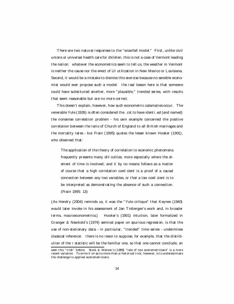
There are two natural responses to the "snowfall model." First, unlike civil
unions or universal health care for children, this is not a case of Vermont leading
the nation: whatever the econometrics seem to tell us, the weather in Vermont
is neither the cause nor the e¤ect of UI utilization in New Mexico or Louisiana.
Second, it would be a mistake to dismiss this exercise because no sensible econo-
mist would ever propose such a model: the real lesson here is that someone
could have substituted another, more "plausible," trended series, with results
that seem reasonable but are no more correct.
This doesn’t explain, however, how such econometric calamaties occur. The
venerable Yule (1926) is often considered the …rst to have identi…ed (and named)
the nonsense correlation problem - his own example concerned the positive
correlation between the ratio of Church of England to all British marriages and
the mortality rates - but Frain (1995) quotes the lesser known Hooker (1901),
who observed that:
The application of the theory of correlation to economic phenomena
frequently presents many di¢culties, more especially where the el-
ement of time is involved; and it by no means follows as a matter
of course that a high correlation coe¢cient is a proof of a causal
connection between any two variables, or that a low coe¢cient is to
be interpreted as demonstrating the absence of such a connection.
(Frain 1995: 13)
(As Hendry (2004) reminds us, it was the "Yule critique" that Keynes (1940)
would later invoke in his assessment of Jan Tinbergen’s work and, in broader
terms, macroeconometrics.) Hooker’s (1901) intuition, later formalized in
Granger & Newbold’s (1974) seminal paper on spurious regression, is that the
use of non-stationary data - in particular, "trended" time series - undermines
classical inference: there is no reson to suppose, for example, that the distrib-
ution of the t statistic will be the familiar one, so that one cannot conclude, on
seen this "trick" before. Stock & Watson’s (1988) "tale of two econometricians" is a morerecent variation. To write it o¤ as no more than a rhetorical trick, however, is to underestimatethe challenge to applied econometricians.
14
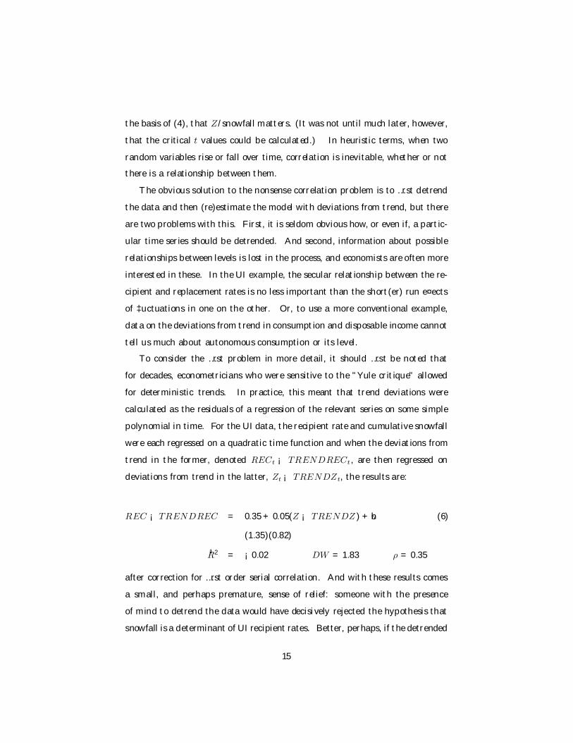
the basis of (4), that Z/snowfall matters. (It was not until much later, however,
that the critical t values could be calculated.) In heuristic terms, when two
random variables rise or fall over time, correlation is inevitable, whether or not
there is a relationship between them.
The obvious solution to the nonsense correlation problem is to …rst detrend
the data and then (re)estimate the model with deviations from trend, but there
are two problems with this. First, it is seldom obvious how, or even if, a partic-
ular time series should be detrended. And second, information about possible
relationships between levels is lost in the process, and economists are often more
interested in these. In the UI example, the secular relationship between the re-
cipient and replacement rates is no less important than the short(er) run e¤ects
of ‡uctuations in one on the other. Or, to use a more conventional example,
data on the deviations from trend in consumption and disposable income cannot
tell us much about autonomous consumption or its level.
To consider the …rst problem in more detail, it should …rst be noted that
for decades, econometricians who were sensitive to the "Yule critique" allowed
for deterministic trends. In practice, this meant that trend deviations were
calculated as the residuals of a regression of the relevant series on some simple
polynomial in time. For the UI data, the recipient rate and cumulative snowfall
were each regressed on a quadratic time function and when the deviations from
trend in the former, denoted RECt ¡ TRENDRECt , are then regressed on
deviations from trend in the latter, Zt ¡ TRENDZt, the results are:
REC ¡ TRENDREC = 0.35 + 0.05(Z ¡ TRENDZ ) + bu (6)
(1.35)(0.82)
¹R2 = ¡0.02 DW = 1.83 ρ = 0.35
after correction for …rst order serial correlation. And with these results comes
a small, and perhaps premature, sense of relief: someone with the presence
of mind to detrend the data would have decisively rejected the hypothesis that
snowfall is a determinant of UI recipient rates. Better, perhaps, if the detrended
15

replacement rate is added to the model, the results are:
REC ¡ TRENDREC = ¡0.10 ¡ 0.97(Z ¡ T RENDZ) + 3.76(REP ¡ T RENDREP )
(1.29) (0.79) (1.04)
¹R2 = 0.19 DW = 1.48 ρ = 0.40
Snowfall still doesn’t matter - even if the rejection is much less emphatic than
it was in (6) - but replacement rates do.
To situate Granger & Newbold’s (1974) contribution, reconsider the funda-
mental premise of this exercise, that all of the variables are stationary around
some deterministic trend or, as this property is sometimes called, trend station-
ary. This means that each time series Xt can be decomposed into the sum of (at
least) two parts, TRENDt + CY CLEt , where T REN Dt is some non-random
function, more often than not of time, and CY CLEt is an autocorrelated series
with mean zero and …nite and constant variance. In the case of cumulative
snowfall, for example, TRENDt was estimated to be 25.7 + 2.55t ¡ 0.002t2 for
t = Y EAR ¡ 1950. As a consequence, the best forecast of Xt+k in period t
tends to T RENDt+k, its trend value, as k increases. In other wrods, the e¤ects
of CY CLEt are assumed to wear out over time, a formulation that reinforces
the (too) sharp distinction between the short and long runs that is characteristic
of much empirical research.
But as some Vermonters would put it, no one but a "‡atlander" would model
cumulative snowfall as a trend stationary process: last winter’s substantial
snows have increased forecasts of cumulative snowfall one, …ve, ten or even …fty
years from now the same amount. Conventional wisdom about winter is better
represented as:
Zt ¡ Zt¡1 = θZ + ut (7)
where θZ can be viewed as "normal" annual snowfall and ut as the annual
surplus or de…cit relative to this norm, an example of a random walk with (no
16

pun intended) drift. This can be rewritten, after repeated substitution, as Zt =
Z0+tθZ +Pt¡1
j=0 ut+j or even TRENDt +CY CLEt , where T RENDt = Z0+tθZ
and CY CLEt =Pt¡1
j=0 ut+j. The similarities to the previous decomposition are
more cosmetic than real, however. The trend component is not deterministic,
but random, since the value of Z0 must itself be random. And the remainder,Pt¡1
j=0 ut+j , cannot be stationary, since the mean is zero but the variance is
neither constant nor, for that matter, even bounded: limt!1 E(Pt¡1
j=0 ut+j)2 =
limt!1 t E(u2) = 1 as t ! 1.
Under these conditions, cumulative snowfall will be di¤erence stationary,
however: ¢Zt will be stationary, with mean θZ and variance E(u2t ). In broader
terms, it is said that a series Xt is integrated of order d, written Xt » I(d), if
its dth di¤erence is stationary: in this case, Zt » I(1). Linear functions of I(1)
variables will of course be I(1) and, with an important class of exceptions to
be discussed later, a linear combination of I(1) variables will also be I(1). (In
fact, if Xt » I(d) and Yt » I(e), then αXt + βYt » I(f ), where f = max[d, e].)
This has two important implications. First, if RECt is also I(1), the re-
searcher must contend with the modern version of the Yule critique, the problem
of spurious regression. In what would soon become "one of the most in‡uential
Monte Carlo studies of all time" (Phillips 1997, p. 273), Granger & Newbold
(1974) constructed 100 pairs of independent I(1) variables and found that in
simple bivariate regressions, the hypothesis that the slope coe¢cient was zero
was rejected (at the 5% level) almost 80 percent of the time for conventional
critical values of the t statistic. In addition, they found that in most cases,
the R2 was surprisingly high, but the Durbin-Watson statistic, the usual mea-
sure of serial correlation, was low, and this combination is still considered an
important, if informal, diagnostic. (It should be noted, therefore, that the …rst
results for (3) should have sounded the alarm: the R2 is 0.86 but the DW is
about 1.) Granger recalls that when he …rst presented the results in a seminar
at LSE, they were "met with total disbelief ...[t]heir reaction was that we must
have gottten the Monte Carlo wrong, [that] we must have done the program-
ming wrong" so that if "I had been part of the LSE group, they might well have
17
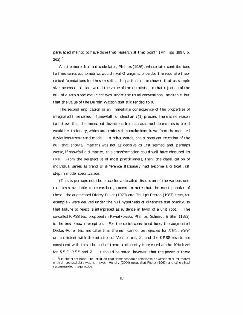
persuaded me not to have done that research at that point" (Phillips, 1997, p.
262).5
A little more than a decade later, Phillips (1986), whose later contributions
to time series econometrics would rival Granger’s, provided the requisite theo-
retical foundations for these results. In particular, he showed that as sample
size increased, so, too, would the value of the t statistic, so that rejection of the
null of a zero slope coe¢cient was, under the usual conventions, inevitable, but
that the value of the Durbin Watson statistic tended to 0.
The second implication is an immediate consequence of the properties of
integrated time series: if snowfall is indeed an I(1) process, there is no reason
to believe that the measured deviations from an assumed deterministic trend
would be stationary, which undermines the conclusions drawn from the modi…ed
deviations-from-trend model. In other words, the subsequent rejection of the
null that snowfall matters was not as decisive as …rst seemed and, perhaps
worse, if snowfall did matter, this transformation could well have obscured its
role! From the perspective of most practitioners, then, the classi…cation of
individual series as trend or di¤erence stationary had become a critical …rst
step in model speci…cation.
(This is perhaps not the place for a detailed discussion of the various unit
root tests available to researchers, except to note that the most popular of
these - the augmented Dickey-Fuller (1979) and Phillips-Perron (1987) tests, for
example - were derived under the null hypothesis of di¤erence stationarity, so
that failure to reject is interpreted as evidence in favor of a unit root. The
so-called KPSS test proposed in Kwiatkowski, Phillips, Schmidt & Shin (1992)
is the best known exception. For the series considered here, the augmented
Dickey-Fuller test indicates that the null cannot be rejected for REC , REP
or, consistent with the intuition of Vermonters, Z , and the KPSS results are
consistent with this: the null of trend stationarity is rejected at the 10% level
for REC, REP and Z . It should be noted, however, that the power of these5 On the other hand, the intuition that some economic relationships were better estimated
with di¤erenced data was not novel. Hendry (2004) notes that Fisher (1962) and others hadrecommended the practice.
18

tests in small samples and against "local alternatives" if often poor, an issue
that will be revisited later.)
If, on this basis, the relationship between recipient rates and cumulative
snowfall is estimated in …rst di¤erences, the results are:
¢REC = ¡0.52 ¡ 0.19¢Z + ut (8)
(4.01) (1.61)
¹R2 = 0.00 DW = 2.09 ρ = ¡0.14
after correction for serial correlation. The rejection of the pure snowfall model
is no less decisive than it was when deviations from some deterministic trend
were used. If the …rst di¤erences in replacement rates and the duration of un-
employment are then added to the model, the results become:
¢REC = ¡0.41 ¡ 0.18¢Z + 4.67¢REP + u
(3.62) (1.44) (0.93) (9)
¹R2 = 0.33 DW = 1.89 ρ = 0.09
Snowfall is still statistically insigni…cant at any level and the in‡uence of the
replacement rate is, in a limited sense, con…rmed. (The caveat would lose
some of its force if the second result survived the addition of other plausible
determinants of UI claim behavior.)
As mentioned earlier, the second problem with models based on transformed
data, whether deviations from deterministic trend or …rst di¤erences, is that
information about relationships between levels is lost. If the data are trend
stationary, the problem is easily solved: it is an implication of the Frisch-
Waugh (1933) Theorem, perhaps better known as the partialling out result,
that the addition of a time trend to a model is equivalent to the transformed
model in which each variable is instead detrended.
If the data are di¤erence stationary, the problem is more complicated, and it
is Granger’s solution, and his appreciation for its broad(er) implications, rather
19
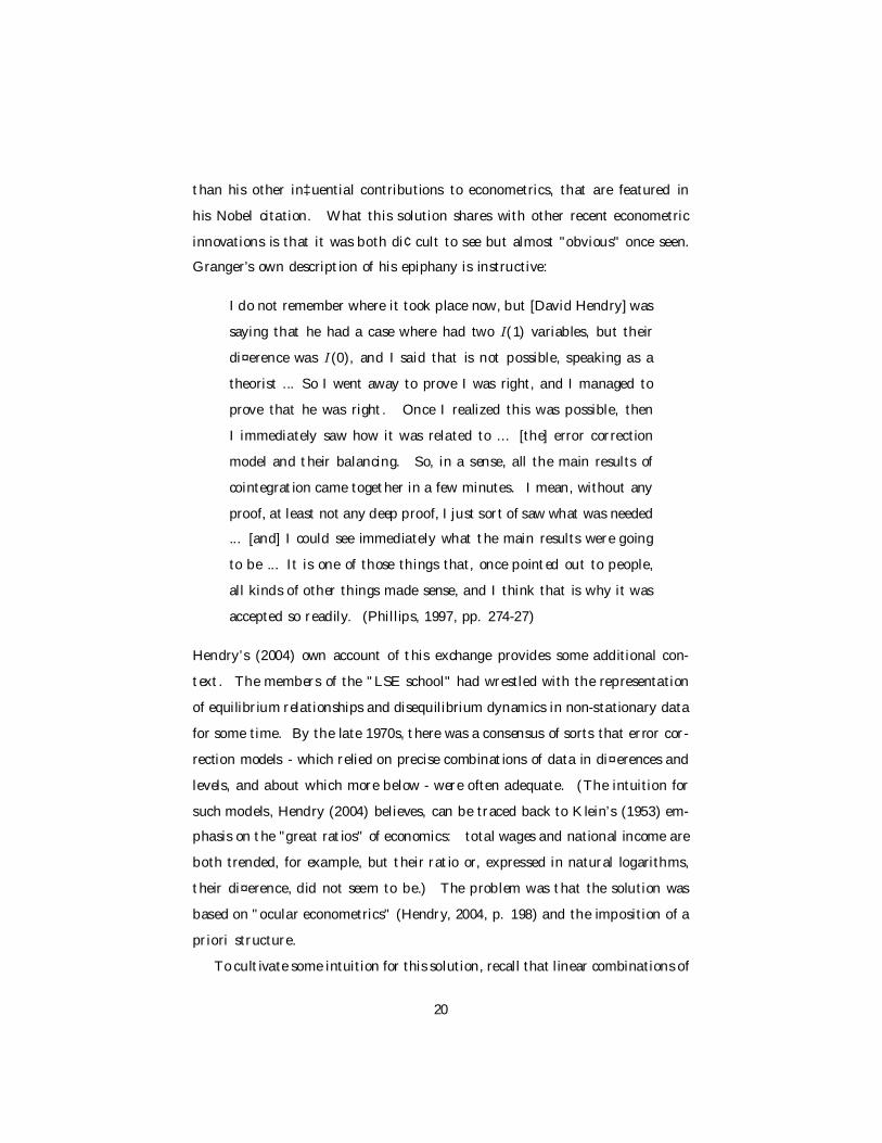
than his other in‡uential contributions to econometrics, that are featured in
his Nobel citation. What this solution shares with other recent econometric
innovations is that it was both di¢cult to see but almost "obvious" once seen.
Granger’s own description of his epiphany is instructive:
I do not remember where it took place now, but [David Hendry] was
saying that he had a case where had two I(1) variables, but their
di¤erence was I(0), and I said that is not possible, speaking as a
theorist ... So I went away to prove I was right, and I managed to
prove that he was right. Once I realized this was possible, then
I immediately saw how it was related to ... [the] error correction
model and their balancing. So, in a sense, all the main results of
cointegration came together in a few minutes. I mean, without any
proof, at least not any deep proof, I just sort of saw what was needed
... [and] I could see immediately what the main results were going
to be ... It is one of those things that, once pointed out to people,
all kinds of other things made sense, and I think that is why it was
accepted so readily. (Phillips, 1997, pp. 274-27)
Hendry’s (2004) own account of this exchange provides some additional con-
text. The members of the "LSE school" had wrestled with the representation
of equilibrium relationships and disequilibrium dynamics in non-stationary data
for some time. By the late 1970s, there was a consensus of sorts that error cor-
rection models - which relied on precise combinations of data in di¤erences and
levels, and about which more below - were often adequate. (The intuition for
such models, Hendry (2004) believes, can be traced back to Klein’s (1953) em-
phasis on the "great ratios" of economics: total wages and national income are
both trended, for example, but their ratio or, expressed in natural logarithms,
their di¤erence, did not seem to be.) The problem was that the solution was
based on "ocular econometrics" (Hendry, 2004, p. 198) and the imposition of a
priori structure.
To cultivate some intuition for this solution, recall that linear combinations of
20
nonstationary I(1) variables are, as a rule, also I(1), so that Granger’s suspicions
about Hendry’s claim were, in some sense, well-founded. This means, for
example, that if Yt and Xt are both I(1), the linear combination Yt ¡ βXt =
α + ut - that is, the combination embedded in the classical linear model - will
also be I(1), as will (therefore) the error term ut . In the absence of some sort of
"equilibrium relationship" between Yt and Xt, the two series will therefore tend
to drift apart from one another over time. But if there is such a relationship,
some sort of mechanism that prevents such drift, there will exist one (and, in
this case, no more than one) combination such that Yt ¡ βXt , and therefore
ut , will be stationary or I(0). In this special case, the two variables are said to
be cointegrated, the term that Granger (1981) coined almost two decades ago.
To be more precise, the vector of N random variables Xt = (X1t ,X 2
t , ..., XNt )
will be cointegrated of order d,b, denoted Xt » CI(d, b), if each X it » I(d)
and there exists some cointegrating vector ¯ = (β1, β2, ..., βN ) such that Zt =PN
i=1 β iX it » I(d ¡ b). There can be at most N ¡ 1 such vectors, each of
them unique up to a scale factor, but there will often be fewer. The most
common procedures to determine this number, and therefore the number of
equilibrium relationships, are those described in Johansen (1988), another pre-
eminent contributor to the literature. So in the simple bivariate case, if Yt
and Xt are both I(1), then each will be non-stationary in levels but stationary
in …rst di¤erences, but if, in addition, (Yt , Xt) is CI(1, 1), then some linear
combination Yt ¡ βXt will also be stationary.
Murray’s (1994) variation on the drunkard’s walk metaphor, the standard
illustration of the most famous I(1) process, the random walk, provides some
homespun intuition. In the parable of the "drunk and the dog," it is impossible
to predict where the next steps of either will take them - in which case the best
forecast of whether each will be a few hours from now is where each started,
which isn’t much of a prediction - unless the dog is hers, in which case the two
never drift far apart. It will still be di¢cult to predict where the pair will be,
but the distance between them will be stationary. Or, in other words, their
paths will be cointegrated.
21

From this intuition comes the almost "obvious" test for cointegration …rst
proposed in Engle & Granger (1987), perhaps the most cited paper in either
laureate’s vita. In terms of UI claim behavior, if RECt and REPt are CI(1, 1),
it should be that RECt ¡ α ¡ βREPt = ut is not I(1) but I(0) - that is,
stationary - for some β. We do not know the "true" value of β or observe
the "true" errors ut , but there are natural proxies for both, namely the least
squares estimates and the associated residuals. The Engle-Granger test is, in
e¤ect, a unit root test of the residuals, where rejection of the null (di¤erence
stationarity) is interpreted as (indirect, to be sure) evidence of cointegration.
In this case, it is di¢cult to reject - for some speci…cations of the test, it can be
rejected at the 10% level, but no lower - so that the evidence of an equilibirum
relationship between REC and REP is, at best, mixed. (This shouldn’t come
as much of a surprise: this is, after all, a "toy model.")
The Granger Representation Theorem, …rst articulated in Granger and Weiss
(1983), then provides the desired relationship between levels and (…rst or other)
di¤erences of cointegrated time series. As the previous quotation and the sub-
sequent discussion both hinted, the connection can be described in terms of the
error correction models or ECMs that predated this work. (The most familiar
ECM is perhaps the DHSY model of consumption (Davidson, Hendry, Srba &
Yeo, 1978) but (the other) Phillips’ (1957) much earlier work on stabilization is
another example.)
To illustrate, consider a dynamic version of the simple bivariate model, Yt =
γ0 + γ1Xt + γ2Yt¡1 + γ3Xt¡1 + et , which has the steady state equilibrium
Y = α + βX , where α = γ0/(1 ¡ γ2) and β = (γ1 + γ3)/(1 ¡ γ2). It is not
di¢cult to show that the model can be rewritten as:
¢Yt = γ1¢Xt + (γ2 ¡ 1)(Yt¡1 ¡ α ¡ βXt¡1) + et (10)
This is the so-called error correction form: period-to-period ‡uctuations in Yt
depend both on ‡uctuations in Xt and the extent to which the model was in
disequilibrium the previous period, Yt¡1 ¡ α ¡ βXt¡1. If (Yt, Xt) » CI(1, 1),
22

then all of the variables in the ECM are I(0) and its coe¢cients can be estimated
with standard (classical) methods. If Yt and Xt are not cointegrated, on the
other hand, then Yt¡1 ¡α¡βXt¡1 will not be stationary, and classical methods
are inappropriate.
To provide a more formal statement of the theorem, recall that if the N
random variables Xt » CI(d,b), there will exist some r£ N matrix B of rank r
such that the r random variables Zt = B0Xt » I(0). (This is just a restatement
of the previous de…nition, where the rows of B0 are the cointegrating vectors.)
Now suppose that the evolution of Xt can be modelled as a vector autoregression
of order k , denoted V AR(k), a generalization of the dynamic model in the
previous paragraph:
Xt = ® + Á1Xt¡1 + Á2Xt¡2 + ... + ÁkXt¡k + ²t (11)
where ® is a column vector, and Á1, ..., Ák square matrices, of coe¢cients. The
theorem asserts that there will exist an N £ r matrix A such that:
I ¡ Á1 ¡ Á2¡... ¡ Ák= AB0 (12)
and k ¡ 1 square matrices ª1, ª2, ..., ªk¡1 such that:
¢Xt = ª1¢Xt¡1+ª2¢Xt¡2 +...+ªk¡1¢Xt¡k+1 +® ¡ AB0Xt¡1+ ²t (13)
which is the multivariate version of the error correction model.6
For the UI data, the equation we are most interested in is:
¢RECt = α1 + λ1(β1RECt¡1 + β2REPt¡1) +Pk¡1
i=1 γ i1¢RECt¡i (14)
+Pk¡1
i=1 γ i2¢REPt¡i + ε1t
where β1RECt¡1 +β2REPt¡1 or, after normalization, RECt¡1¡β 2REPt¡1, is
often understood as last period’s deviation from equilibrium, and the parameter
λ1 measures the speed of adjustment.6 This is the version of the theorem, or at least part of it, presented in Hamilton’s (1994)
useful text.
23

Engle & Granger’s (1987) two step estimator for (14) was the …rst, and re-
mains the simplest, available to time series econometricians. Building on the
work of Stock (1987), who showed that least squares estimates of the cointe-
grating vector [β1, β2] were superconsistent - that is, converged more rapidly
than usual - they demonstrated that if these estimates were substituted into
the ECM and the values of the other paramaters α1, λ1, γ11, ..., γ
k¡11 ,γ1
2, ..., γk¡12
estimated via maximum likelihood, the results would be both consistent and
asymptotically normal.
The Johansen (1988) test reveals, however, that the evidence that RECt and
REPt are cointegrated is at best mixed. Nevertheless, for k = 4, the maximum
likelihood estimate of the (standardized) cointegrating vector is [1, 5.67], while
the estimate of λ1 is ¡0.12. So if an equilibrium relationship does exist, the
speed of adjustment is quite slow, consistent with the view that in the short
run, ‡uctuations in the replacement rate can drive claim behavior far from its
eventual "equilibrium." This said, the …tted values of the estimated ECM track
the observed …rst di¤erences remarkably well, as illustrated in Figure 8.
[Insert Figure 8 About Here]
Three extensions of the CI framework deserve special mention in this con-
text. Hylleberg, Engle, Granger & Yoo (1990) introduced the notion of seasonal
cointegration. Granger & Lee (1989) developed multicointegration to model
stock-‡ow relationships. In their example, if sales and output are CI(1, 1) then
the di¤erence, or investment in inventories, will be stationary, but the stock of
inventories will not be. If the stock of inventories and sales are also cointe-
grated, however, then sales and output will be multicointegrated. And Granger
& Swanson (1995) have considered nonlinear cointegration.
4 A Few Words About Causality and Prediction
Granger (1986) was also the …rst to notice an important connection between
CI models and his own much earlier work (Granger, 1969) on causality. In
24

particular, he perceived that if a pair of economic time series was cointegrated,
then one of them must Granger cause the other. Most readers will recall
that the de…nition of Granger causality embodies two crucial axioms (Granger,
1987): uniqueness, which is the principle that the "cause" contain unique
information about the "e¤ect," and strict temporal priority. In operational
terms, this amounts to a condition on prediction variance: in crude terms, if
one stationary time series is better predicted with a second series than without
it, the latter is said to cause the former. It was not Granger’s (1969) paper
that launched a thousand cauality test ships, however, but rather Sims’ (1972):
regressing the logarithm of current nominal GNP on a number of its own lags
and lags of the logarithm of either "broad money" or the monetary base, and
then vice versa, he famously concluded that "money causes income" but that
"income does not cause money." A little more three decates later, empirical
macroeconomists continue to publish variations on this simple exercise, among
them a number of post Keynesians who believe - mistakenly, it seems to me -
that the debate with the mainstream about the endogeneity of money, or for
that matter the internal debate between structuralist and accommodationist
explanations of endogeneity, will be resolved on this basis.7 Granger himself
remains ambivalent about Sims’ (1972) paper. Much later, he would observe
that "part of the defense of the people who did not like the conclusion of [this]
paper was that this was not real causality, this was only ’Granger causality’ [and]
they kept using the phrase ... everywhere in their writings, which I thought was
very ine¢cient, but ... made my name very prominent" (Phillips, 1997, p.
272). More important, he believes that the most common form of the test,
based on a comparison of in sample …ts, violates the spirit, and perhaps the
letter, of his own de…nition, which emphasizes the importance of (out of sample)
predictability.
7 The most impressive example of this literature is perhaps Palley (1994), who uses Grangercausality tests to evaluate the orthodox, structuralist and accommodationist approaches, con-cluding that the evidence favors the last of these.
25
If Granger’s (1969) causality paper is the most visible of his other contribu-
tions to econometric theory, it remains his most controversial. Tobin’s (1970)
sharp reminder of the perils of post hoc ergo propted hoc reasoning in economics
was written in response to Friedman and Schwartz (1963), but it can also be read
as a critique of the later Sims (1972). It was for this reason that Leamer (1985)
would recommend that econometricians substitute "precedence" for "causality."
In a similar vein, Zellner (1979) dismisses the notion that causal relations can
be de…ned, or detected, without respect to economic laws.
Granger himself remains unrepentant. He believes that the test - the intu-
ition for which is found outside economics, in the work of the mathematician
Norbert Weiner - is "still the best pragmatic de…nition [or] operational de…ni-
tion" (Phillips, 1997, p. 272). And he believes that the philosphers have started
to come around:
The philosophers ... initially did not like this de…nition very much,
but in recent years several books on philosophy have discussed it in
a much more positive way, not saying that it is right, but also saying
that it is not wrong. I view that as supporting my position that it
is probably a component of what eventually will be a de…nition of
causation that is sound. (Phillips, 1997, p. 272)
At the least, Granger’s paper remains the point of departure for most "prag-
matic" discussions of causality in economics, a number of which (Hoover, 2001,
for example) have produced viable extensions or alternatives. It is also embed-
ded in other econometric concepts: it is part, for example, of the de…nition of
strong exogeneity (Engle, Hendry & Richard, 1983).
In some sense, Granger’s research on causality can be viewed as a particular
manifestation of his interest in prediction or forecasting, one that he shares with
co-laureate Engle. Published at the same time as the (now, if not then) better
known causality paper, for example, Bates & Granger (1969) were the …rst to
prove the once counterintuitive result that pooled forecasts tend to perform
better than individual ones. For those familiar with James Surowiecki’s recent
26

The Wisdom of Crowds (2004), the intuition is similar: pooled forecasts allow
di¤erential biases to o¤set one another. And in the last few years, Granger
(2001) has returned to the problem of forecast evaluation.
Diebold (2004, p. 169) believes that "Engle’s preference for parametric, par-
simonious models [also re‡ects a] long-standing concern with forecasting ...[that]
guard against in-sample over…tting or data mining," but adds that he is also
responsible for several more speci…c contributions to the literature. Engle &
Yoo (1987), for example, was one of the …rst papers to explore the properties of
forecasts made on the basis of cointegrated systems. From a broader perspec-
tive, the whole ARCH framework can be understood as an attempt to produce
better forecasts, or at least better estimates of forecast error variances.
5 Trouble In Paradise?
It seems reasonable to suppose that with the increased attention that ARCH
and CI models have received since the Royal Academy’s announcement, more
economists outside the mainstream will be tempted to experiment with one or
both. There is reason to be cautious, however. The most important opera-
tional criticism of the common trends framework, for example, is that testing
for unit roots or estimating cointegrating vectors is problematic in small(ish)
samples. For the researcher armed with annual, or even quarterly, data, for ex-
ample, the bene…ts are uncertain. Miron (1991, p. 212), himself a contributor
to the technical literature, believes that "since we can never know whether the
data are trend stationary or di¤erence stationary [in …nite samples], any result
that relies on the distinction is inherently uninteresting." The implicit advice,
that researchers should …t both sorts of models to time series data, even in those
cases where test results seem decisive, strikes (at least) me as sound. For the
UI claim data, for example, the conclusion that recipient and replacement rates
share a common trend, or that short run ‡uctuations in replacement rates are
associated with substantial movements in claims, is a more robust one than it
would have been if both alternatives had not been considered.
27

One of the most persuasive illustrations of this problem is Perron’s (1989)
paper on unit root tests in a world which, if trend stationary, is trend stationary
with structural breaks. It is important to appreciate that at the time the paper
was published, the conventional wisdom held that almost all macroeconomic
time series were either I(1) or I(2): Nelson & Plosser’s (1982) often cited
article, for example, found that for 13 of 14 series - the one exception was the
unemployment rate - the null hypothesis of a unit root could not be rejected.
The immediate and widespread success of Engle and Granger (1987), which
provided researchers with a tractable framework for the analysis of relationships
between such series, owed at least a little to this near consensus. What Perron
(1991) showed, however, was that if one allowed for just two structural breaks
- what he describes as the "intercept shift" of the Great Crash of 1929 and
the "slope shift" of the oil price shock of 1973 - around an otherwise stable,
trend stationary, process, the unit root hypothesis could now be rejected for
11 of the same 14 series! While later studies have quali…ed Perron’s reversal -
Zivot & Andrews (1992), for example, endogenized the selection of breakpoints
and found that 6 of the 14 series were not di¤erence stationary - the lesson for
empirical researchers, heterodox or otherwise, is clear: there is still much to be
learned from old fashioned, if more ‡exible, decompositions of economic time
series.
ARCH models su¤er from their own small sample woes, as Engle himself
understood from the beginning (Engle, Hendry & Richard, 1985). On the
basis of their own Monte Carlo studies, for example, Hwang and Periera (2003)
…nd that at least 250 observations are required to o¤set the bias problem in
ARCH(1) models, and more than 500(!) in GARCH(1,1) models. This is
seldom a constraint with daily, or even weekly, …nancial market data, but it
represents a very long time indeed when the data source is annual state UI
reports!
(At this point, little is known about the interaction of these small sample
problems. Mantalos (2001) …nds, however, that I(1) series with GARCH(1, 1)
errors, the null hypothesis tends to be overrejected or, in other words, that
28
cointegration is detected more often than it should be.)
A second practical concern about ARCH/GARCH models is related to their
common, and sometimes lucrative, application to …nancial market data. The
most important of these involve the use of conditional variances to improve es-
timates of value at risk, as embodied in J. P. Morgan’s in‡uential RiskMetrics
paradigm. In this context, it is important to ask how well this class of models
capture the stylized facts of asset markets. It has already been observed, for
example, that clustered volatility and the information release e¤ect can be rep-
resented, and it can be shown that another variant, Nelson’s (1991) EGARCH,
can accommodate a leverage e¤ect.8 But there is some evidence (Brock & Pot-
ter, 1993, Brock & de Lima, 1996) that there is otherwise unmodelled nonlinear
structure in …nancial data.
The contribution of ARCH/GARCH models to the "new …nancial economet-
rics" raises broader questions, however, about the existence of such structure.
In a recent critique, Mayer (1999), for example, observes that "[Basle’s] abdi-
cation of supervisory function followed J. P. Morgan’s publication of its Risk-
Metrics methodology, which supposedly enabled banks to measure the extent of
their risks looking forward into the realm where uncertainty, not of probability,
reigns" (emphasis added).
Concerns about statistical inference in a world where outcomes are uncertain,
rather than probabilistic, extend to CI models, too. Davidson (1994) is perhaps
the most prominent of the post Keynesians to assert that economic processes are
nonergodic and thus nonstationary, and that this di¤erence cannot be "undone"
with the use of di¤erenced data. If true, the structure uncovered in such models
will often be an artifact. Lawrence Klein, the Nobel laureate who for decades
embodied the older Cowles Commission approach to macroeconometrics, shares
a practical concern about the (over)use of di¤erences, if not the post Keynesian
premise:
I do not think economic data are necessarily stationary or that
8 EGARCH models were one of the …rst asymmetric conditional variance models, and allowthe volatilties of positive and negative shocks to di¤er.
29

economic processes are stationary. The technique of cointegration,
to keep di¤erencing the data until stationarity is obtained and then
relate the stationary series, I think can do damage. It does damage
in the sense that it almost always done on a bivariate or maybe
trivariate basis. That keeps the analysis simple ... but the world is
not simple.
[I] would conclude that one should accept the fact that economic
data are not stationary, relate the non-stationary data, but include
the explicit [deterministic] trends and think about what could cause
the trends in the relationship. One then uses that more complicated
relationship with trend variables. Successive di¤erencing, as it is
done in cointegration techniques, may introduce new relationation-
ships, some of which we do not want to have in our analysis (Klein,
1994, p. 34, emphasis added)
Klein (1994, p. 34) also expresses some unease that the "youngest ... generation
of econometricians simply do [this] mechanically ... and do not understand the
original data series as well as they should."
The heterodox economist who is still tempted to use the CI framework must
also consider its unfortunate - but I believe inessential - link to the "real business
cycle" or RBC paradigm. The near consensus that once existed that almost all
macro time series were I(1) or I(2) but that subsets of these formed cointegrated
systems was, and to some extent still is, linked to the rise of RBC models. (I
am tempted to add that if, as some believe, the term "heterodox" is too broad
to be useful, the widespread rejection of such models could be the exception
that proves the rule.) The reason is not di¢cult to infer: if real output has
a "strong unit root," for example, then one could interpret its evolution over
time in terms of a series of permanent shocks or, as Shapiro & Watson (1988)
concluded, as random increases in potential income, rather than a sequence of
transitory shocks around some deterministic trend/potential. Furthermore, as
King, Plosser, Stock & Watson (1988, p. 320) reminded their readers, in the
30

presence of technology shocks, "balanced growth under uncertainty implies that
consumption, investment and output [will be] integrated."
There are at least two reasons to suppose that the connection is more tenuous
than …rst seems, however. First, as De Long & Summers (1988) have observed,
the strength of the unit root in real output is in some measure an artifact, a
consequence of macroeconomists’ preoccupation with post World War II data.
(Of course, to the extent that earlier data is either unavailable or unreliable, the
preoccupation is an understandable one.) Viewed from this perspective, the
diminished importance of "transitory ‡uctuations" in this period has less to do
with RBCs that with the success of old fashioned Keynesianism at stabilization,
a point also made, albeit in a di¤erent context, by Tobin (1982).
The second is that whether or not balanced growth is su¢cient for cointegra-
tion, it does not follow that it is also necessary. It is not clear that old fashioned
Keynesianism, or any other heterodox approach, requires that the evolution of
critical time series be limited to stationary ‡uctuations around some determin-
istic trend. It is not clear to me, for example, that the existence of a stochastic
trend is incompatible with some sort of Harrodian, or demand driven, model of
economic growth.
There is another, more subtle, explanation for this connection, one that is
related to current methodological debates in econometrics. The recent concern
over the use of incredible restrictions as a means of identi…cation, the fashion for
"unrestricted" vector autoregressions, the interest in cointegrating vectors and
ECMs and, to a lesser extent, the use of ARCH models can all be understood
as manifestations of the LSE or general-to-speci…c approach to empirical re-
search. Like "rational" expectations, however, general-to-speci…c is not always
the unalloyed virtue it …rst seems. For each new variable added to an ECM,
for example, there is a substantial increase in the number of new parameters to
estimate, a mild version of the curse of dimensionality. (To assume a priori
that some of these coe¢cients are zero is, of course, to impose the sort of re-
strictions that "old fashioned" econometricians have relied on for decades.) As
a result, most CI or ECM models tend to be parsimonious and while there are
31

no doubt exceptions to the rule, the models of orthodox economists tend to be
"lower dimensional" than those of their heterodox counterparts (Pandit 1999).
If in‡ation is "always and everywhere a monetary phenomenon," for example,
then a bivariate VAR is su¢cient for many purposes! Pandit (1999) also cites
Klein (1999) as a source of examples of cases in which parsimonious models lead
to incorrect conclusions.
6 Conclusion
It is not uncommon for some outside the mainstream to remind us that the Bank
of Sweden’s prize for "economic science" is newer than, and di¤erent from, the
other Nobels, or to protest that it resembles a "beauty contest" that some kinds
of contestants will never win. There is some truth to this, of course: the failure
to award the prize to Joan Robinson, for example, is still incomprehensible. To
dismiss the achievements of those who have won, however, because of those who
haven’t is facile. More than a few laureates have challenged, and sometimes
informed, various heterodox traditions. It would be naive to claim, for example,
that the in‡uence of Arrow, who shared the 1972 prize, Leontief (1973), Myrdal
(1974), Lewis (1979), Tobin (1981), Nash (1994), Sen (1998), Akerlof (2001) or
Stiglitz (2001) were limited to the mainstream.
Should Engle and/or Granger be added to this illustrious list? However
durable their technical accomplishments prove, there is little doubt that each
has in‡uenced how we think about and sometimes organize economic data.
7 References
Atesoglu, H. S. (2000) Income, employment, in‡ation and money in theUnited States, Journal of Post Keynesian Economics, 22, pp. 639-646.
Atesoglu, H. S. (2002) Stock prices and employment, Journal of Post Key-nesian Economics, 24, pp. 493-498.
Banarjee, A. & Hendry, D. F. (1992) Testing integration and cointegration:an overview, Oxford Economic Papers, 54, pp. 225-255.
32

Bates, J. M. & Granger, C. W. J. (1969) The combination of forecasts,Operations Research Quarterly, 20, pp. 451-468.
Blank, R. & Card, D. (1991) Recent trends in insured and uninsuredunemployment: is there an explanation? Quarterly Journal of Economics, 106,pp. 1157-1189.
Bollerslev, T., Engle, R. F. & Wooldridge, J. M. (1986) A capital assetpricing model with time-varying covariances, Journal of Political Economy, 96,pp. 116-131.
Bollerslev, T. (1986) Generalized autoregressive conditional heteroscedastic-ity, Journal of Econometrics, 31, pp. 307-327.
Brock, W. & Potter, S. (1993) Nonlinear time series and macroeconomet-rics, in: G. S. Maddala, C. R. Rao & H. D. Vinod (Eds) Handbook of Statistics,11, pp. 195-229.
Brock, W. & De Lima, P. (1995) Nonlinear time series, complexity theoryand …nance, in: G. S. Maddala & C. R. Rao (Eds) Handbook of Statistics, 14.
Campbell, J. Y. & Shiller, R. J. (1987) Cointegration and tests of presentvalue models, Journal of Political Economy, 95, pp. 1062-1088.
Davidson, J. E. H., Hendry, D. F., Srba, F. & Yeo, S. (1978) Econometricmodelling of the aggregate time-series relationship between consumers’ expen-diture and income in the United Kingdom, Economic Journal, 88, pp. 661-692.
Davidson, P. (1991) Is probability theory relevant for uncertainty: a postKeyensian perspective, Journal of Economic Perspectives, 5, pp. 129-143.
De Long, J. B. & Summers, L. (1988) On the existence and interpretationof a "unit root" in US GDP, NBER Working Paper, 2716.
Dickey, D. A. & Fuller, W. A. (1979) Distribution of the estimators forautoregressive time series with a unit root, Journal of the American StatisticalAssociation, 74, pp. 427-431.
Dickey, D. A., Jansen, D. W. & Thornton, D. L. (1992) A primer on cointe-gration with an application to money and income, Federal Reserve Bank of St.Louis Review, 73, pp. 58-78.
Diebold, F. X. (2003) The ET interview: Professor Robert F. Engle, Econo-metric Theory, 19, pp. 1159-1193.
Diebold, F. X. (2004) The Nobel Memorial Prize for Robert F. Engle,Scandinavian Journal of Economics, 106, pp. 165-185.
33

Ding, Z., Granger, C. W. J. & Engle, R. F. (1993) A long memory propertyof stock market returns and a new model, Journal of Empirical Finance, 1, pp.83-106.
Engle, R. F., Bradbury, K., Irvine, O. & Rothenberg, J. (1977) Simultane-ous estimation of the supply and demand for household location in a multizonedmetropolitan area, in: G. K. Ingram (Ed) Residential Location and Urban Hous-ing Markets (Cambridge, Ballinger).
Engle, R. F. & Granger, C. W. J. (1987) Cointegration and error correction:representation, estimation and testing, Econometrica, 55, pp. 251-276.
Engle, R.F., Granger, C. W. J. & Robins, R. (1986) Wholesale and retailprices: bivariate modeling with forecastable variances, in: D. Belsey and E. Kuh(Eds) Model Reliability (Cambridge, MIT Press).
Engle, R. F., Hendry, D. F. & Richard, J.-F. (1983) Exogeneity, Economet-rica, 51, pp. 277-304.
Engle, R. F., Hendry, D. F. & Trumble, D. (1985) Small-sample propertiesof ARCH estimators are tests, Canadian Journal of Economics, 18, pp. 66-93.
Engle, R. F. & Kraft, D. (1983) Multiperiod forecast error variances ofin‡ation estimated from ARCH models, in A. Zellner (Ed) Applied Time SeriesAnalysis of Economic Data (Washington, Bureau of the Census).
Engle, R. F., Lilien, D. M. & Robins, R. P. (1987) Estimating time varyingrisk premia in the term structure: the ARCH-M model, Econometrica, 55, pp.391-407.
Engle, R. F. & Liu, T. C. (1972) E¤ects of aggregation over time on dynamiccharacteristics of an economic model, in: B. G. Hickman (Ed) Econometric Mod-els of Cyclical Behavior: Studies in Income and Wealth (New York, NationalBureau of Economic Research).
Engle, R. F. & Manganelli, S. (2001) CAViaR: conditional autoregressivevalue at risk by regression quantiles, NBER Working Paper, W7341.
Engle, R. F. & Rosenberg (1995) GARCH gammas, Journal of Derivatives,2, pp. 47-59.
Engle, R. F. & Yoo, B. S. (1987) Forecasting and testing in co-integratedsystems, Journal of Econometrics, 35, pp. 143-159.
Engle, R. F. (1973) Band spectrum regression, International EconomicReview, 15, pp. 1-11.
34
Engle, R. F. (1974a) Issues in the speci…cation of an econometric model ofmetropolitan growth, Journal of Urban Economics, 1, pp. 250-267.
Engle, R. F. (1974b) A disequilibrium model of regional investment, Journalof Regional Science, 14, pp. 367-376.
Engle, R. F. (1976) Policy pills for a metropolitan economy, Papers andProceedings of the Regional Science Association, 35, pp. 191-205.
Engle, R. F. (1982) Autoregressive conditional heteroscedasticity with es-timates of the variance of United Kingdom in‡ation, Econometrica, 50, pp.987-1007.
Fisher, F. M. (1962) A Priori Information and Time Series Analysis (Am-sterdam, North-Holland).
Frain, J. (1995) Econometrics and truth, Bank of Ireland Technical Paper,2/RT/95.
French, K. R., Schwert, W. G. & Stambaugh, R. F. (1987) Expected stockreturns and volatility, Journal of Finance, 19, pp. 3-29.
Friedman, M. & Schwartz, A. (1963) Monetary History of the United States,1870-1960 (Princeton, Princeton University Press).
Frisch, R. & Waugh, F. V. (1933) Partial time regression as compared withindividual trends, Econometrica, 1, pp. 221-223.
Granger, C. W. J. (1957) A statistical model for sunspot activity, Astro-physical Journal, 126, pp. 152-158.
Granger, C. W. J. (1959) Estimating the probability of ‡ooding on a tidalriver, Journal of the Institution of Water Engineers, 13, pp. 165-174.
Granger. C. W. J. (1969) Investigating causal relations by econometricmodels and cross-spectral methods, Econometrica, 37, pp. 424-438.
Granger, C. W. J. (1981) Some properties of time series data and their usein econometric model speci…cation, Journal of Econometrics, 16, pp. 121-130.
Granger, C. W. J. (1986) Developments in the study of cointegrated eco-nomic variables, Oxford Bulletin of Economics and Statistics, 48, pp. 213-228.
Granger, C. W. J. (1987) Causal inference, in: J. Eatwell, M. Milgate andP. Newman (Eds) The New Palgrave: Econometrics (New York, Norton).
35

Granger, C. W. J. (2001) Evaluation of forecasts, in: D. F. Hendry & N. R.Ericsson (Eds) Understanding Economic Forecasts (Cambridge, MIT Press).
Granger, C. W. J. & Anderson, A. P. (1978) Introduction to Bilinear TimeSeries Models (Gottingen, Vandenhoeck & Ruprecht).
Granger, C. W. J. & Bates, J. (1969) The combination of forecats, Opera-tions Research Quarterly, 20, pp. 451-468.
Granger, C. W. J., Craft, M. & Stephenson, G. (1964) The relationship be-tween severity of personality disorder and certain adverse childhood in‡uences,British Journal of Psychiatry, 110, pp. 392-396.
Granger, C. W. J. & Hatanaka, M. (1964) Spectral Analysis of EconomicTime Series (Princeton, Princeton University Press).
Granger, C. W. J. & Joyeux, R. (1980) An introduction to long-memorytime series models and fractional di¤erencing, Journal of Time Series Analysis,1, pp. 15-30.
Granger, C. W. J. & Lee, T.H. (1989) Investigation of production, salesand inventory relationships using multicointegration and non-symmetric errorcorrection models, Journal of Applied Econometrics, 4, pp. 145-159.
Granger, C. W. J. & Newbold, P. (1974) Spurious regression in econometrics,Journal of Econometrics, 2, pp. 111-120.
Granger, C. W. J. & Swanson, N. R. (1995) Further developments in thestudy of cointegrated variables, Oxford Bul letin of Economics and Statistics, 58,pp. 537-553.
Granger, C. W. J. & Weiss, A. A. (1983) Time series analysis of errorcorrection models, in: S. Karlin, T. Amemiya & L. A. Goodman (Eds) Studiesin Econometrics, Time Series and Multivariate Statistics in Honor of T. W.Anderson (San Diego, Academic Press).
Hamilton, J. D. (1994) Time Series Analysis (Princeton, Princeton Univer-sity Press).
Hendry, D. F. (1977) On the time series approach to econometric modelbuilding, in: C. A. Sims (Ed) New Methods in Business Cycle Research (Min-neapolis, Federal Reserve Bank).
Hendry, D. F. (2004) The Nobel Memorial Prize for Clive W. J. Granger,Scandinavian Journal of Economics, 106, pp. 187-213.
36
Hooker, R. H. (1901) Correlation of the marriage rate with trade, Journalof the Royal Statistical Society, 64, pp. 485-492.
Hoover, K. (2001) Causality in Macroeconomics (Cambridge, CambridgeUniversity Press).
Hwang, S. & Periera, P. L. V. (2003) Small sample properties of GARCHestimates and persistence, Imbec Finance Lab Working Paper.
Hylleberg, S., Engle, R. F., Granger, C. W. J. & Yoo, B. S. (1990) Seasonalcointegration, Journal of Econometrics, 44, pp. 215-238.
Johansen, S. (1988) Statistical analysis of cointegrating vectors, Journal ofEconomic Dynamics and Control, 12, pp. 231-254.
Keynes, J. M. (1940) Comment, Economics Journal, 50, pp. 154-156.
King, R. G., Plosser, C. I., Stock, J. H. & Watson, M. W. (1991) Stochastictrends and economic ‡uctuations, American Economic Review, 81, pp. 819-840.
Klein, L. R. (1954) A Textbook of Econometrics (Evanston, Row, Peterson& Company).
Klein, L. R. (1994) Problems with modern economics, Atlantic EconomicJournal, 22, pp. 34-39.
Klein, L.R. (1999) Economic stabilization policy: pitfalls of parsimoniousmodelling, Journal of Quantitative Economics,15.
Kwiatkowski, D., Phillips, P. C. B., Schmidt, P. & Shin, T. (1992) Testingthe null hypothesis of stationarity against the alternative of a unit root: howsure are we that economic series have a unit root? Journal of Econometrics, 54,pp. 159-178.
Leamer, E. E. (1985) Vector autoregressions for causal inference? CarnegieRochester Conference Series on Public Policy, 22, pp. 255-303.
Lopez G. J. & Cruz, A. B. (2000) Thirlwall’s Law and beyond: the LatinAmerican experience, Journal of Post Keynesian Economics, 22, pp. 477-495.
Loranger, J-G. (2001) Structural form of an accumulation model: an analy-sis of cointegration of the long term growth of the Canadian economy, Universityof Montreal Working Paper.
Mantalos, P. (2001) ECM-cointegration tests with GARCH(1,1) errors,Interstat, March 2001. Online at http://interstat.stat.vt.edu/InterStat/.
37
Matthews, P. H., Kandilov, I. T. & Maxwell, B. (2002) Interstate di¤erencesin insured unemployment: some recent evidence, Applied Economics Letters, 9,pp. 945-948.
Mayer, M. (1999) Somebody turn on the lights, Derivatives Strategy,November.
Miron, J. (1991) Comment, NBER Macroeconomics Annual, pp. 211-219.
Mizon, G. E. (1995) Progressive modelling of macroeconomic time series, in:K. D. Hoover (Ed) Macroeconometrics: Developments, Tensions and Prospects(Boston, Kluwer).
Murray, M. (1994) A drunk and her dog: an illustration of cointegrationand error correction, The American Statistician, 48, pp. 37-39.
Nelson, C. R. & Plosser, C. I. (1982) Trends and random walks in macro-economic time series, Journal of Monetary Economics, 10, pp. 139-162.
Nelson, D. B. (1991) Conditional heteroscedasticity in asset returns: a newapproach, Econometrica, 59, pp. 347-390.
Palley, T. (1994) Competing views of the money supply process: theory andevidence, Metroeconomica, 45, pp. 67-88.
Pandit, V. (1999) Structural modelling under challenge, Center for Devel-opment Economics/Delhi School of Economics Working Paper, 98.
Perron, P. (1989) The great crash, the oil price shock, and the unit roothypothesis, Econometrica, 57, pp. 1361-1401.
Phelps, E. (1988) Comment on recent developments in macroeconomics,Journal of Money, Credit and Banking, 20, pp. 456-458.
Phillips, A. W. (1957) Stabilization policy and the time forms of laggedresponses, Economic Journal, 67, pp. 265-277.
Phillips, P. C. B. (1986) Understanding spurious regressions in econometrics,Journal of Econometrics, 33, pp. 311-340.
Phillips, P. C. B. (1997) The ET interview: Professor Clive Granger, Econo-metric Theory,13, pp. 253-303.
Phillips, P. C. B. & Perron, P. (1987) Testing for a unit root in a time seriesregression, Biometrika, 75, pp. 335-346.
38
Rappaport, P. & White, E. N. (1993) Was there a bubble in the 1929 stockmarket? Journal of Economic History, 53, pp. 549-574.
Shapiro, M. D. & Watson, M. W. (1988) Sources of business cycle ‡uctua-tions, NBER Macroeconomics Annual, pp. 111-148.
Shiller, R. J. (2003) From e¢cienct markets theory to behavioral …nance,Journal of Economic Perspectives, 17, pp. 83-104.
Sims, C. A. (1972) Money, income and causality, American Economic Re-view, 62: 540-552.
Stock, J. H. (1987) Asymptotic properties of least squares estimators ofcointegrating vectors, Econometrica, 55, pp. 1035-1056.
Stock, J. H. & Watson, M. W. (1988) Variable trends in economic timeseries, Journal of Economic Perspectives, 2, pp. 141-174.
Surowiecki, J. (2004) The Wisdom of Crowds (New York, Random House).
Taylor, A. (1995) International capital mobility in history: purchasing-powerparity in the long run, NBER Working Paper, 5742.
Tobin, J. (1970) Money and income: post hoc ergo propter hoc? QuarterlyJournal of Economics, 94, pp. 301-317.
Tobin, J. (1982) Asset Accumulation and Economic Activity: Re‡ections onContemporary Macroeconomic Theory (Chicago, University of Chicago Press).
Yule, G. U. (1926) Why do we sometimes get nonsense correlations betweeentime series? A study in the sampling and nature of time series, Journal of theRoyal Statistical Society, 89, pp. 1-6.
Zacharias, A. (2001) Testing pro…t rate equalization in the US manufactur-ing sector: 1947-1998, Jerome Levy Institute Working Paper.
Zellner, A. (1979) Causality and econometrics, Carnegie Rochester Serieson Public Policy, 10, pp. 9-54.
Zivot, E. and Andrews, D. W. K. (1992) Further evidence on the GreatCrash, oil price shock and the unit root hypothesis, Journal of Business andEconomic Statistics, 10, pp. 251-270.
39

0.5
11
.52
2.5
De
nsi
ty
-.4 -.2 0 .2 .4 .6Rate of Return
Figure 1. Rates of Return in the Stock Market 1871-2002

0.0
5.1
.15
.2.2
5R
etu
rn
1850 1900 1950 2000Year
Figure 2. Squared Returns in the Stock Market 1871-2002
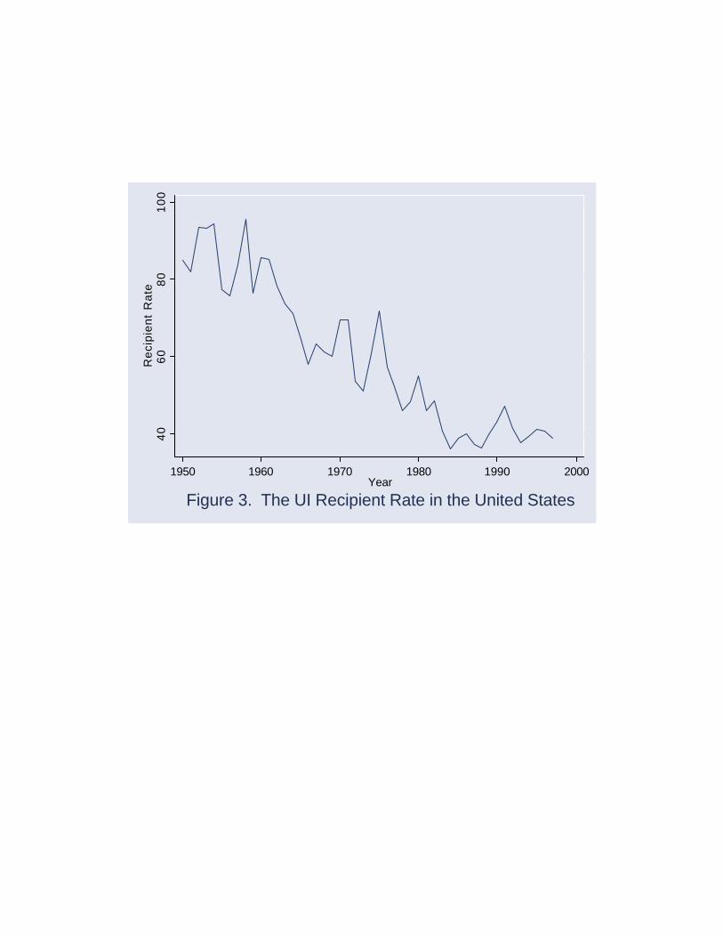
40
60
80
10
0R
eci
pie
nt
Ra
te
1950 1960 1970 1980 1990 2000Year
Figure 3. The UI Recipient Rate in the United States

-20
-10
01
0C
ha
ng
e in
Re
cip
ien
t R
ate
1950 1960 1970 1980 1990 2000Year
Figure 4. Actual and Predicted Changes in Recipient Rates

05
01
00
15
02
00
Sq
ua
red
Re
sid
ua
ls
1950 1960 1970 1980 1990 2000Year
Figure 5. Squared Residuals From Simple Model
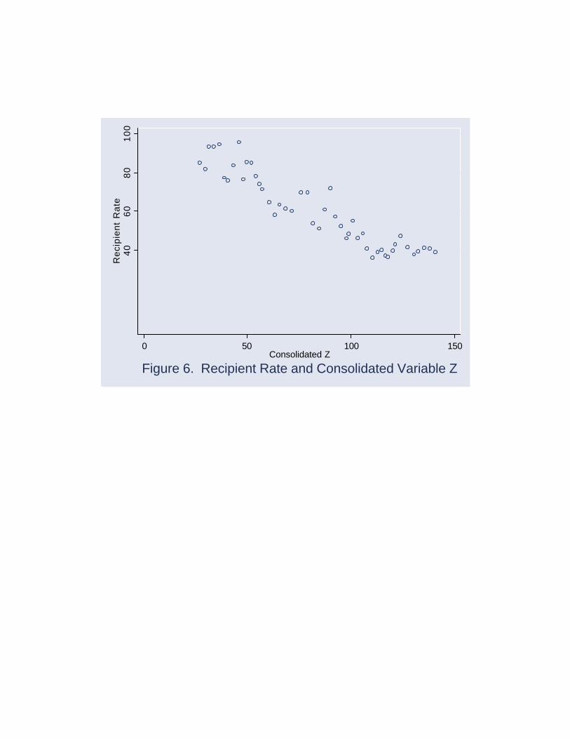
40
60
80
10
0R
eci
pie
nt
Ra
te
0 50 100 150Consolidated Z
Figure 6. Recipient Rate and Consolidated Variable Z

40
60
80
10
0R
eci
pie
nt
Ra
te (
%)
1950 1960 1970 1980 1990 2000Year
Actual Forecast
Figure 7. Actual and Forecast Recipient Rates/Bivariate Model

-20
-10
01
0F
irst
Diff
ere
nce
in
Re
cip
ien
t R
ate
1950 1960 1970 1980 1990 2000year
Actual Observed
Figure 8. Observed and Predicted Differences in ECM

![CWS ParadiseLine. · 2019-04-02 · 12 ] Paradise Air Bar 13 ] Paradise Seatcleaner 14 ] Paradise Toiletpaper 15 ] Paradise Superroll 16 ] Paradise Paper Bin 17 ] Paradise Ladycare](https://cdn.vdocuments.us/doc/165x107/5f4d115eb47f9811753b5af9/cws-2019-04-02-12-paradise-air-bar-13-paradise-seatcleaner-14-paradise.jpg)


