
Page 1
EXPERT
Study Guide for MOS Objectives (Expert) in Microsoft Excel 2013 Illustrated
1.0 Manage and Share Workbooks
1.1 Manage Multiple Workbooks Pages Where Covered
Modifying existing templates 356 (Step 7 Tip)
Merging multiple workbooks 325 (Clue)
Managing versions of a workbook 353 (Clue)
Copying styles from template to template See MOS reference
Copying macros from workbook to workbook 382 (Clue)
Linking to external data
310 (Steps 1-7), 308 (Steps 1-6), 140 (Steps
1-4), 302 (Steps 1-3), 312 (Steps 1-7), 280
(Step 3 Tip), 332 (Steps 1-3), 336 (Steps 1-3),
334 (Steps 1-6)
1.2 Prepare a Workbook for Review Pages Where Covered
Setting tracking options 326 (Steps 1-6)
Limiting editors
See MOS reference, 328-329, 132-133, 138
(Steps 2-8)
Creating workspaces Removed from Excel 2013
Restricting editing 132 (Steps 1-7)
Controlling recalculation 348 (Steps 1-7)
Protecting worksheet structure 132 (Steps 1-7)
Marking as final 138 (Step 7)
Removing workbook metadata 138 (Steps 1-4)
Encrypting workbooks with a password 328 (Step 1)
1.3 Manage Workbook Changes Pages Where Covered
Tracking changes 326 (Steps 1-7)
Managing comments 352 (Steps 1-8)
Identifying errors 346 (Steps 1-8)
Troubleshooting with tracing 346 (Step 4 Tip), (Steps 5-8)
Displaying all changes 326 (Steps 2-7)
Retaining all changes See MOS reference
2.0 Apply Custom Formats and
Layouts
2.1 Apply Custom Data Formats Pages Where Covered
Creating custom formats (Number, Time, Date) See MOS reference
Creating custom accounting formats See MOS reference
Using advanced Fill Series options 354 (Steps 1-7)
2.2 Apply Advanced Conditional Formatting and FilteringPages Where Covered
Writing custom conditional formats 183 (Clue)
Using functions to format cells See MOS reference
Creating advanced filters 182 (Steps 1-5), 184 (Steps 1-5)
Managing conditional formatting rule 64 (Clue), 181 (Clue)
2.3 Apply Custom Styles and Templates Pages Where Covered
Creating custom color formats See MOS reference
Creating and modifying cell styles See MOS reference
Creating and modifying custom templates 356 (Step 7 Tip), (Steps 1-8)
Creating form fields 217 (Clue)
Page 2
EXPERT
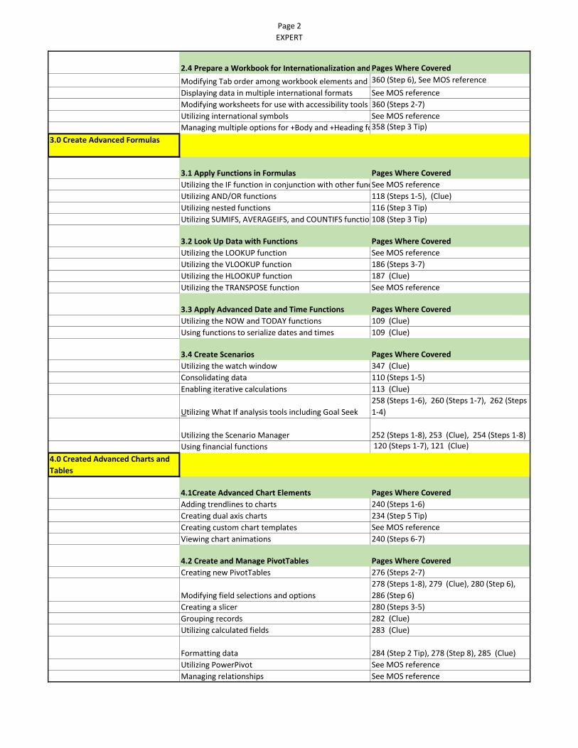
2.4 Prepare a Workbook for Internationalization and AccessibilityPages Where Covered
Modifying Tab order among workbook elements and objects360 (Step 6), See MOS reference
Displaying data in multiple international formats See MOS reference
Modifying worksheets for use with accessibility tools 360 (Steps 2-7)
Utilizing international symbols See MOS reference
Managing multiple options for +Body and +Heading fonts358 (Step 3 Tip)
3.0 Create Advanced Formulas
3.1 Apply Functions in Formulas Pages Where Covered
Utilizing the IF function in conjunction with other functionsSee MOS reference
Utilizing AND/OR functions 118 (Steps 1-5), (Clue)
Utilizing nested functions 116 (Step 3 Tip)
Utilizing SUMIFS, AVERAGEIFS, and COUNTIFS functions108 (Step 3 Tip)
3.2 Look Up Data with Functions Pages Where Covered
Utilizing the LOOKUP function See MOS reference
Utilizing the VLOOKUP function 186 (Steps 3-7)
Utilizing the HLOOKUP function 187 (Clue)
Utilizing the TRANSPOSE function See MOS reference
3.3 Apply Advanced Date and Time Functions Pages Where Covered
Utilizing the NOW and TODAY functions 109 (Clue)
Using functions to serialize dates and times 109 (Clue)
3.4 Create Scenarios Pages Where Covered
Utilizing the watch window 347 (Clue)
Consolidating data 110 (Steps 1-5)
Enabling iterative calculations 113 (Clue)
Utilizing What If analysis tools including Goal Seek
258 (Steps 1-6), 260 (Steps 1-7), 262 (Steps
1-4)
Utilizing the Scenario Manager 252 (Steps 1-8), 253 (Clue), 254 (Steps 1-8)
Using financial functions 120 (Steps 1-7), 121 (Clue)
4.0 Created Advanced Charts and
Tables
4.1Create Advanced Chart Elements Pages Where Covered
Adding trendlines to charts 240 (Steps 1-6)
Creating dual axis charts 234 (Step 5 Tip)
Creating custom chart templates See MOS reference
Viewing chart animations 240 (Steps 6-7)
4.2 Create and Manage PivotTables Pages Where Covered
Creating new PivotTables 276 (Steps 2-7)
Modifying field selections and options
278 (Steps 1-8), 279 (Clue), 280 (Step 6),
286 (Step 6)
Creating a slicer 280 (Steps 3-5)
Grouping records 282 (Clue)
Utilizing calculated fields 283 (Clue)
Formatting data 284 (Step 2 Tip), 278 (Step 8), 285 (Clue)
Utilizing PowerPivot See MOS reference
Managing relationships See MOS reference

Page 3
EXPERT
4.3 Create and Manage Pivot Charts Pages Where Covered
Creating new PivotCharts 286 (Steps 2-8)
Manipulating options in existing PivotCharts 286 (Steps 5-8)
Applying styles to PivotCharts 286 (Step 4 Tip)
Microsoft Office Specialist (MOS) Reference: Excel 2013 (EXPERT)
Study Guide for additional MOS skills Page 1 of 10 For Microsoft Excel 2013 Illustrated Complete
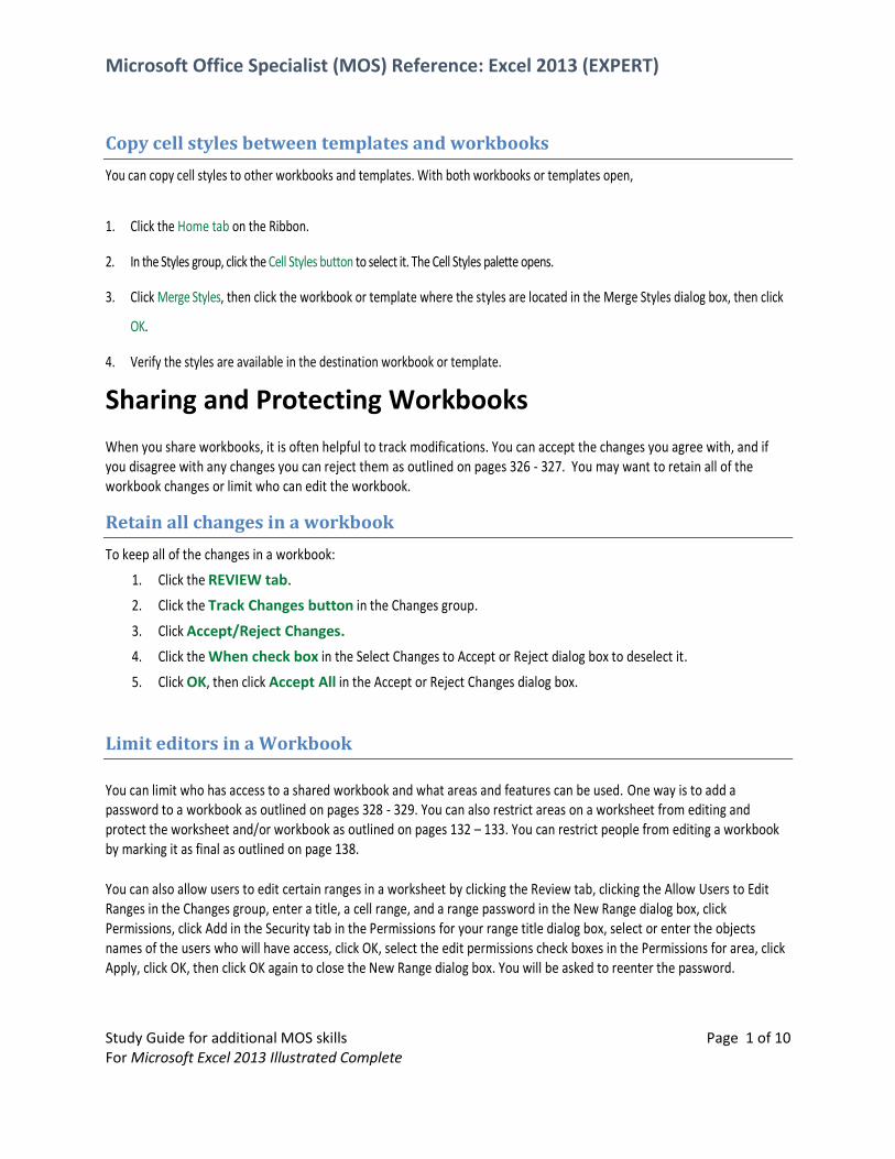
Copy cell styles between templates and workbooks
You can copy cell styles to other workbooks and templates. With both workbooks or templates open,
1. Click the Home tab on the Ribbon.
2. In the Styles group, click the Cell Styles button to select it. The Cell Styles palette opens.
3. Click Merge Styles, then click the workbook or template where the styles are located in the Merge Styles dialog box, then click
OK.
4. Verify the styles are available in the destination workbook or template.
Sharing and Protecting Workbooks
When you share workbooks, it is often helpful to track modifications. You can accept the changes you agree with, and if you disagree with any changes you can reject them as outlined on pages 326 - 327. You may want to retain all of the workbook changes or limit who can edit the workbook.
Retain all changes in a workbook
To keep all of the changes in a workbook:
1. Click the REVIEW tab.
2. Click the Track Changes button in the Changes group.
3. Click Accept/Reject Changes.
4. Click the When check box in the Select Changes to Accept or Reject dialog box to deselect it.
5. Click OK, then click Accept All in the Accept or Reject Changes dialog box.
Limit editors in a Workbook
You can limit who has access to a shared workbook and what areas and features can be used. One way is to add a password to a workbook as outlined on pages 328 - 329. You can also restrict areas on a worksheet from editing and protect the worksheet and/or workbook as outlined on pages 132 – 133. You can restrict people from editing a workbook by marking it as final as outlined on page 138.
You can also allow users to edit certain ranges in a worksheet by clicking the Review tab, clicking the Allow Users to Edit Ranges in the Changes group, enter a title, a cell range, and a range password in the New Range dialog box, click Permissions, click Add in the Security tab in the Permissions for your range title dialog box, select or enter the objects names of the users who will have access, click OK, select the edit permissions check boxes in the Permissions for area, click Apply, click OK, then click OK again to close the New Range dialog box. You will be asked to reenter the password.

Microsoft Office Specialist (MOS) Reference: Excel 2013 (EXPERT)
Study Guide for additional MOS skills Page 2 of 10 For Microsoft Excel 2013 Illustrated Complete
Creating custom number, time, date, and accounting
formats
When you use numbers, times and dates in worksheets or calculations, you can apply the Excel custom number formats, or create
your own custom formats. To apply a custom cell format, click the HOME tab, click the Format button in the Cells group, then click
Format Cells. If necessary, click the Number tab in the Format Cells dialog box, click Custom in the Category list, then click the
format you want. A number format can have four parts, each one separated by semicolons: [positive numbers];[negative
numbers];[zeroes];[text]. You don’t need to specify all four parts. Many of the custom formats contain codes: # represents any
digit and 0 represents a digit that will always be displayed, even if the digit is 0. An underscore adds space for alignment of positive
numbers and negative numbers enclosed in parentheses. For example, the value -1234.65 appears as (1,235) if the cell is
formatted as #,##0 _); (#,##0).
You can also use custom date and time formats. For example 2/28/2016 appears as 28-Feb if the cell is formatted as d-mmm and
5:00 appears as 5:00:00 if the cell is formatted as [h]:mm:ss. To create your own custom format, click a format that resembles the
one you want and customize it in the Type text box. For example, you could edit the #,##0_);[Red](#,##0) format to show negative
numbers in blue by changing it to read #,##0_);[Blue](#,##0).
You can also customize the Accounting format by beginning with a cell formatted with the Accounting format, click the HOME tab,
click the Format button in the Cells group, then click Format Cells. If necessary, click the Number tab in the Format Cells dialog box,
click Custom in the Category list, your format will be displayed in the Type text box, then edit the format to the accounting format
you wish to customize. For example entering 123.45 and formatting it as Accounting, the following is displayed in the Type
textbox: _($* #,##0.00_);_($* (#,##0.00);_($* "-"??_);_(@_). If you prefer to display negative numbers in red, you can edit the
Type to: _($* #,##0.00_);[Red]_($* (#,##0.00);_($* "-"??_);_(@_)
Using functions to format cells
You can use a function to conditionally format cells in a worksheet. For example, if you have a column of
invoice dates and you want to format the dates that are overdue, you can use the TODAY() function in a
conditional formatting rule. In the figure below, the dates are in the range A1:A9.
Format cells using the TODAY function
1. Select the dates that will be formatted (In this example A1:A9.)
2. Click the HOME tab, click the Conditional Formatting button in the Styles group, then click New
Rule.
3. Click Use a formula to determine which cells to format in the New Formatting Rule dialog box.
4. Enter the formula seen in the Format values where this formula is true text box in the figure
below, then click Format.
Microsoft Office Specialist (MOS) Reference: Excel 2013 (EXPERT)
Study Guide for additional MOS skills Page 3 of 10 For Microsoft Excel 2013 Illustrated Complete
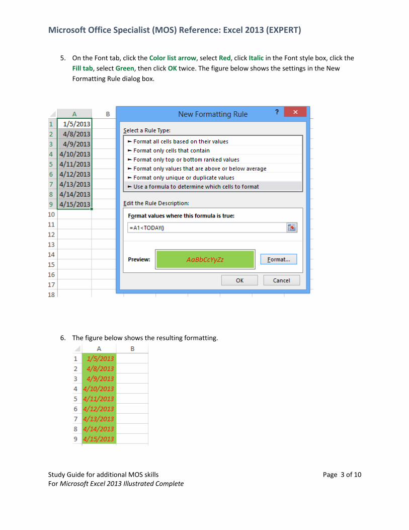
5. On the Font tab, click the Color list arrow, select Red, click Italic in the Font style box, click the
Fill tab, select Green, then click OK twice. The figure below shows the settings in the New
Formatting Rule dialog box.
6. The figure below shows the resulting formatting.

Microsoft Office Specialist (MOS) Reference: Excel 2013 (EXPERT)
Study Guide for additional MOS skills Page 4 of 10 For Microsoft Excel 2013 Illustrated Complete
Creating Custom Color Formats
You can create custom color formats for fills or fonts.
Create a custom color format
1. Click the Home tab on the Ribbon.
2. In the Cells group, click the Format list arrow, then click Format Cells. The Format Cells dialog box opens.
3. Click the Fill or Font tab, (On the Font tab click the Color list arrow) click More Colors, click the Custom tab, enter the RGB
color codes or click to create a color, then click OK twice.
The colors will be available in the bottom of the color palette under Recent Colors.
Create new cell styles
1. Click the Home tab on the Ribbon.
2. In the Styles group, click the Cell Styles button to select it. The Cell Styles palette opens.
3. Click New Cell Style. The Style dialog box opens.
4. Type a name in the Style Name text box, then select or deselect style options from the Style Includes (By Example)
list.
5. Click the Format button to choose customized formatting for your style, then click
OK twice.
Modify cell styles
1. Click the Home tab on the Ribbon.
2. In the Styles group, click the Cell Styles button to select it. The Cell Styles palette opens.
3. Right-click the cell style that you want to modify, then click Modify on the shortcut menu. The Style dialog box
opens.
4. Verify the style name in the Style name text box, then select or deselect style options from the Style Includes (By
Example) list.
5. Click the Format button to choose new customized formatting for the style, then click

Microsoft Office Specialist (MOS) Reference: Excel 2013 (EXPERT)
Study Guide for additional MOS skills Page 5 of 10 For Microsoft Excel 2013 Illustrated Complete
OK twice.
Utilizing international formats and symbols
Excel has many international tools to help you customize your workbooks for use in other countries and
languages.
You can use international currency symbols in Excel by clicking Format on the HOME tab, clicking Format
Cells, then select the Number tab in the Format Cells dialog box, if necessary. Click either the Currency
or Accounting category, click the Symbol list arrow, then click the desired currency symbol.
Excel also has a Euro Currency Tools Add-In that will convert and format your data into the Euro
currency. To add the Euro Currency Tools to your Excel workbooks click the FILE tab, click Options, click
Add-Ins in the Excel Options dialog box, click Euro Currency Tools in the Add-Ins list, then click OK.
You can also use keyboard shortcuts to insert international characters. For example to insert an accent
grave in the French language, press [CTRL] + ` + the letter. For example the letter a with an accent grave
is: à. To display ï you need to press [CTRL] + [SHIFT] + : + the letter i. You can use Microsoft’s Help to
find other international keyboard shortcuts.
You can set your language preferences by clicking the FILE tab, clicking Options, clicking Language in the
Excel Options dialog box, then selecting an editing language, a display and Help language with language
priority for buttons, tabs, and Help, and a ScreenTip language. You can add additional languages for all
of the settings and set the language priority order.
Utilizing the IF function in conjunction with other
functions
You can use the IF function with other functions if you have multiple conditions to test. For example,
below a student receives a passing grade only if both the average and the attendance are 60 or above.
You can use and AND statement to test these two conditions and an IF statement to determine the
grade. The formula is: =IF(AND(B2>=60, C2>=60),"P", "F") and the result is shown below.

Microsoft Office Specialist (MOS) Reference: Excel 2013 (EXPERT)
Study Guide for additional MOS skills Page 6 of 10 For Microsoft Excel 2013 Illustrated Complete
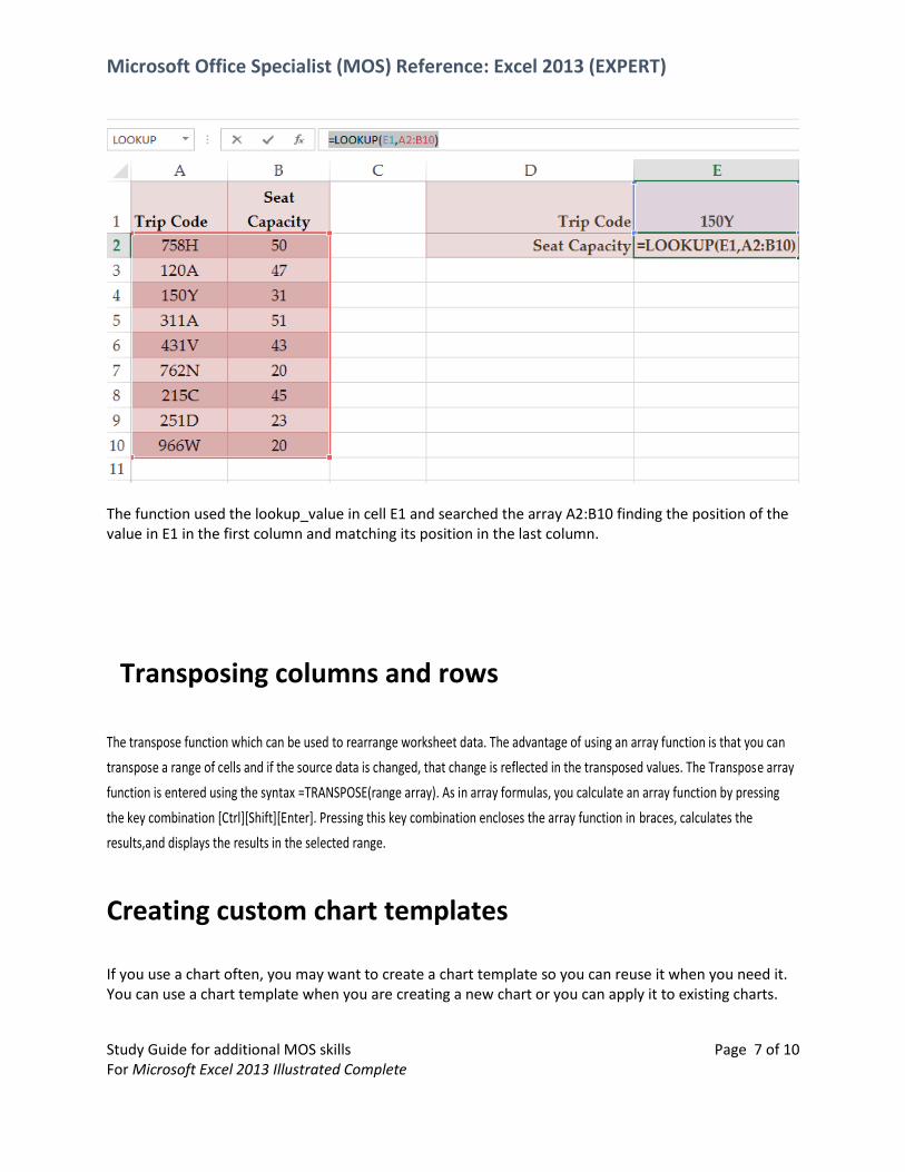
Utilizing the LOOKUP function
You can use the LOOKUP function to find the value at the corresponding position of a range or array. For example, in the range A2:B10 below, you can find the seat capacity in the range B2:B10 for a trip code in the range A2:A10 using the formula: =LOOKUP(E1,A2:A10,B2:B10)
The syntax for the LOOKUP formula is LOOKUP(lookup_value, lookup_vector, [result_vector])
The lookup_value is the value that will be used in the search, the lookup_vector is the range that will be searched for the lookup_value and it can only be one row or one column. These values must be sorted in ascending order because if the value can’t be matched, the function will return the closest value less than the lookup_value. The result_vector is not required. If it is entered, it represents the range which will be used to find the matching position of the value in the lookup_vector. This vector can also be only one row or column and the same size as the lookup_vector.
LOOKUP functions can also be used with arrays. Here the LOOKUP formula searches the first row or column of an array range for the lookup_value, and finds the value at the corresponding position in the array’s last row or column. The syntax is: LOOKUP(lookup_value, array) The example below the same information as above is found using an array of A2:B10 in the LOOKUP function:
=LOOKUP(E1,A2:B10)
Microsoft Office Specialist (MOS) Reference: Excel 2013 (EXPERT)
Study Guide for additional MOS skills Page 7 of 10 For Microsoft Excel 2013 Illustrated Complete
The function used the lookup_value in cell E1 and searched the array A2:B10 finding the position of the value in E1 in the first column and matching its position in the last column.
Transposing columns and rows
The transpose function which can be used to rearrange worksheet data. The advantage of using an array function is that you can
transpose a range of cells and if the source data is changed, that change is reflected in the transposed values. The Transpose array
function is entered using the syntax =TRANSPOSE(range array). As in array formulas, you calculate an array function by pressing
the key combination [Ctrl][Shift][Enter]. Pressing this key combination encloses the array function in braces, calculates the
results,and displays the results in the selected range.
Creating custom chart templates
If you use a chart often, you may want to create a chart template so you can reuse it when you need it. You can use a chart template when you are creating a new chart or you can apply it to existing charts.

Microsoft Office Specialist (MOS) Reference: Excel 2013 (EXPERT)
Study Guide for additional MOS skills Page 8 of 10 For Microsoft Excel 2013 Illustrated Complete
To save a chart as a chart template, right-click the chart, click Save as Template on the shortcut menu, enter the File name in the Save Chart Template dialog box, make sure the location where the chart will be saved is in the Charts folder inside the Templates folder, then click Save. The chart template is saved with a file extension of .crtx.
To apply the template to a new chart, select the data that you want to include in a chart, click the Quick Analysis tool, click CHARTS, click More Charts, then click All Charts in the Insert Chart dialog box. Click Templates in the Insert Chart dialog box, click the template that you want to use in the My Templates section, then click OK.
To apply the template to an existing chart, select the chart, click the CHART TOOLS DESIGN tab, click the Change Chart Type button in the Type group, click the Templates folder, click the chart template in the Change Chart Type dialog box, then click OK. The chart template acts like a custom chart type.
Utilizing PowerPivot
PowerPivot is a data analysis tool built-in to Excel 2013 as an add-in. The add-in is available in Microsoft Office Professional Plus. Before Excel 2013 had the ability to handle large data sets efficiently, PowerPivot was required for this task. PowerPivot in Excel 2013 is used to enhance Excel data models. To enable PowerPivot click FILE, click Options, click Add-Ins, click the Manage list arrow, click COM Add-ins, click Go, click the Microsoft Office PowerPivot for Excel 2013 checkbox to select it, then click OK.
To import Access table data into an Excel workbook using PowerPivot, click the POWERPPIVOT tab, click the Manage button in the Data Model group, click the Get External Data button in the PowerPivot for Excel window, click From Database, click From Access, click Browse in the Table Import Wizard to locate the Access file, click Next, click Next, select the tables for import, select Finish, then click Close after the import is completed. The imported table names are displayed at the bottom of the PowerPivot window. You can click on a table name to see the table data.
The imported data can be formatted and sorted using the Home tab on the PowerPivot sheet. You can also add calculations and change the way data is viewed using these buttons. The Design tab buttons allow you to add additional calculations, work with columns and manage relationships between fields.
Creating and managing Excel data relationships
You can expand the types of data to include in your PT by creating relationships between data in different tables of a PivotTable. To create a relationship in PowerPivot, click the POWERPIVOT tab if necessary, click the Manage button in the Data Model group, click the Design tab, in the PowerPivot for Excel window, click the Create Relationship in the Relationships group, select the Tables and Columns that you want to create a relationship between in the Create Relationship dialog box, then click Create.
Microsoft Office Specialist (MOS) Reference: Excel 2013 (EXPERT)
Study Guide for additional MOS skills Page 9 of 10 For Microsoft Excel 2013 Illustrated Complete
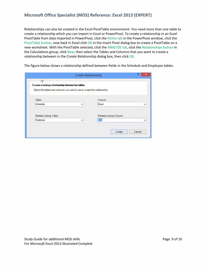
Relationships can also be created in the Excel PivotTable environment. You need more than one table to create a relationship which you can import in Excel or PowerPivot. To create a relationship in an Excel PivotTable from data imported in PowerPivot, click the Home tab in the PowerPivot window, click the PivotTable button, now back in Excel click OK in the Insert Pivot dialog box to create a PivotTable on a new worksheet. With the PivotTable selected, click the ANALYZE tab, click the Relationships button in the Calculations group, click New, then select the Tables and Columns that you want to create a relationship between in the Create Relationship dialog box, then click OK.
The figure below shows a relationship defined between fields in the Schedule and Employee tables.

Microsoft Office Specialist (MOS) Reference: Excel 2013 (EXPERT)
Study Guide for additional MOS skills Page 10 of 10 For Microsoft Excel 2013 Illustrated Complete
The figure below shows a Pivot Table that uses the relationship between two tables, defined in the above figure, to replace employee
numbers with names to show the hours worked.


