
Output high order sliding mode control of unity-power-factor in three-phase
AC/DC Boost Converter
www.utbm.frLaboratoire SeT
JianXing Liu, Salah Laghrouche, Maxim WackLaboratoire Systèmes Et Transports (SET)

Contents of the presentation
www.utbm.fr
Introduction
Problem Formulation
Second order sliding mode controller design
Second order sliding mode observer design
Simulation results with proposed controller
Conclusions

AC-DC power conversion
www.utbm.fr
AC-DC power conversion is required by all electronic devices
virtually
MOSFET, IGBT, are commonly used for AC-DC Converters
The electric utility grid has a sinusoidal waveform, and most electronic equipment needs a DC power supply.

AC-DC power conversion
www.utbm.fr
Power factor reflects the efficiency and quality of such process. Different control algorithms have been used to achieve unity power factor.
An output second order sliding mode control is designed here.
Problem:1. The performance and efficiency of power converters
with unknown varying load and internal uncertainties2. Minimize the number of the sensors

Model of three phase AC/DC converter
www.utbm.fr
Fig1 Three phase boost type AC/DC converter
The circuit of three phase AC/DC boost converterlinki

Model
www.utbm.fr
Model in Phase Coordinate Frame:101
1 1 2 3
2022 2 1 2
33 03 3 1 2
0 01 1 2 2 3 3
(2 )6
(2 )6
(2 )6
1 ( )2
g
g
g
l
UUdi r i u u udt L L L
UUdi r i u u udt L L L
Udi Ur i u u udt L L LdU U u i u i u idt R C C
= − − − − +
= − − − − + = − − − − + = − + + +

Model in (d,q) Coordinate Frame
www.utbm.fr
It is convenient to design the control in the rotating reference frame synchronized with the supply frequency.Transformation Matrix:
1
2
3
2 2cos( ) cos( ) cos( )2 3 32 23 sin( ) sin( ) sin( )3 3
d
q
xt t txx
xt t t x
ω ω π ω π
ω ω π ω π
− + = − − − − +
Define:2 2cos( ) cos( ) cos( )2 3 32 23 sin( ) sin( ) sin( )3 3
t t tC
t t t
ω ω π ω π
ω ω π ω π
− + =
− − − − +
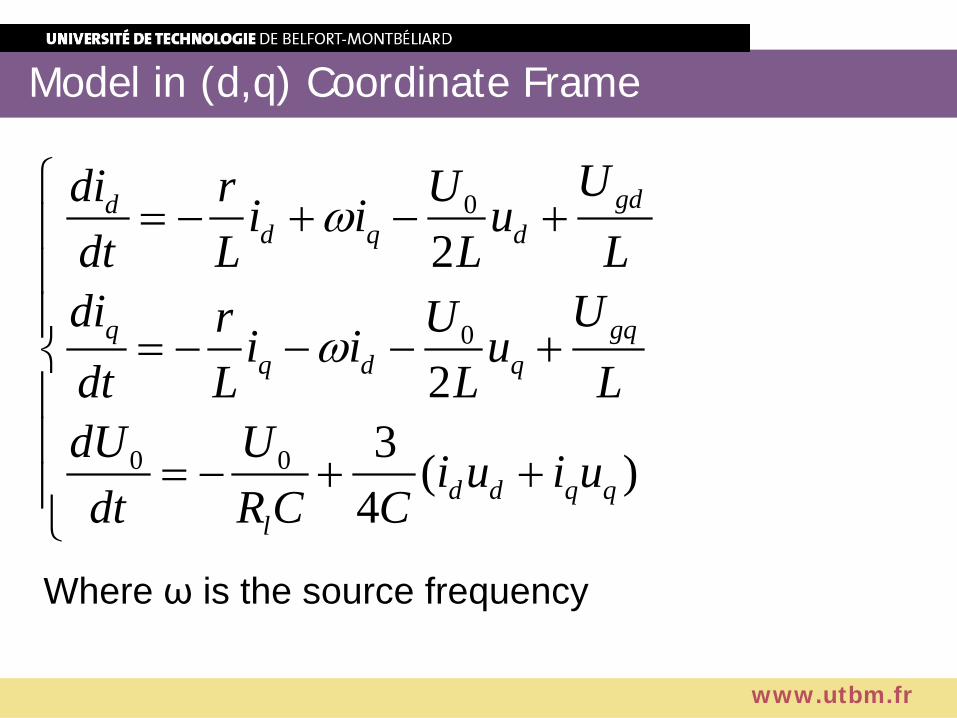
Model in (d,q) Coordinate Frame
www.utbm.fr
Where ω is the source frequency
0
0
0 0
2
23 ( )
4
gddd q d
q gqq d q
d d q ql
Udi Ur i i udt L L Ldi UUr i i udt L L LdU U i u i udt R C C
ω
ω
= − + − +
= − − − + = − + +
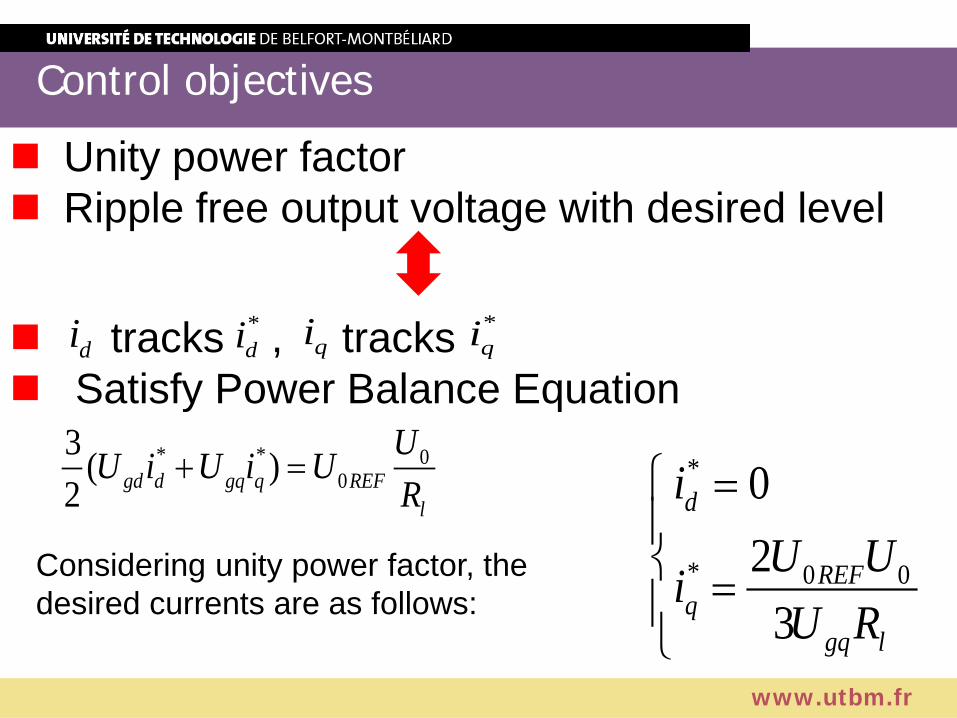
Control objectives
www.utbm.fr
Unity power factor Ripple free output voltage with desired level
tracks , tracks Satisfy Power Balance Equation
di*di qi *
qi
* * 00
3 ( )2 gd d gq q REF
l
UU i U i UR
+ =
Considering unity power factor, the desired currents are as follows:
*
* 0 0
02
3
d
REFq
gq l
iU UiU R
= =
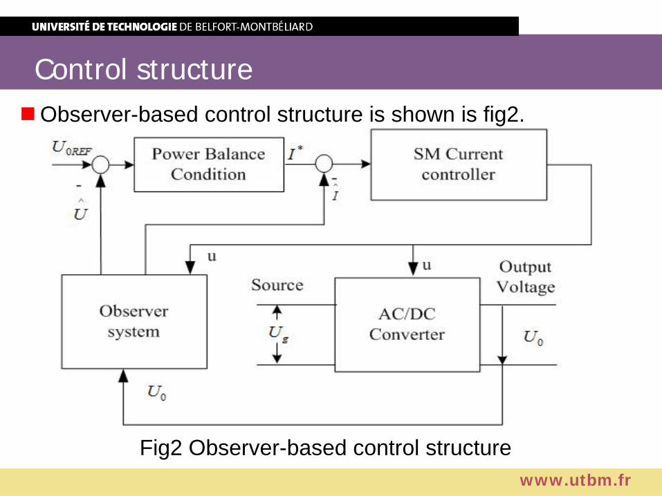
Control structure
www.utbm.fr
Fig2 Observer-based control structure
Observer-based control structure is shown is fig2.

Super-Twisting sliding mode
www.utbm.fr
Robustness property with respect to perturbations and parametric uncertainties.
Smoother than the classic sliding mode control
Advantages:
where , , !nx f b∈( , ) ( , )( )
x f x t b x t uy s x
⋅
= +=
Design12( ), ( ) ( ) ( ) ,( , 0)u s s s sign s sign s dtυ υ λ α λ α= − = + >∫
Control Objective: Force to zero.( )s x
The relative degree with respect to is equal to one.( )s x

Step1:Sliding manifolds design
www.utbm.fr
Design the switching functions:*
*d d d
q q q
s i is i i= −
= −To find a domain in the system space from which any state trajectory converges to the sliding manifold(sd=0,sq=0).
*1
0 02
*3
2 2
gdd d q
d d d
q qgqq q q d
Ur ui i is u fU UL L C uu fU L Lrs i i i u
L L
ω
ω
⋅⋅
⋅ ⋅
− − − = + = + − − +
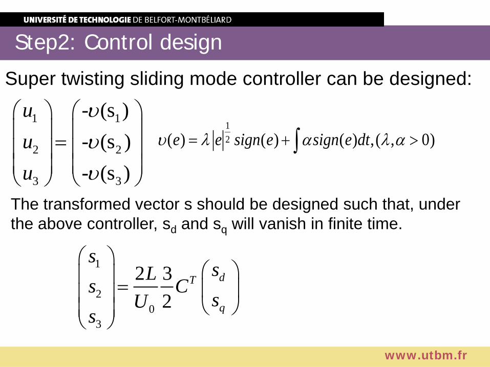
Step2: Control design
www.utbm.fr
Super twisting sliding mode controller can be designed:
12( ) ( ) ( ) ,( , 0)e e sign e sign e dtυ λ α λ α= + >∫
1
20
3
2 32
dT
q
ssLs CsU
s
=
1 1
2 2
3 3
- (s )- (s )- (s )
uuu
υυυ
= The transformed vector s should be designed such that, under the above controller, sd and sq will vanish in finite time.

Super-Twisting Observation Design
www.utbm.fr
Assuming that only the output voltage(U0) is measured, a super-twisting sliding observer is constructed as a copy of the original system.
Define observation error:
1
2
3 0 0
d d
q q
e i i
e i i
e U U
∧
∧
∧
= −
= − = −
01 3
02 3
0 03 3
( )2
( )2
3 ( ) ( )4
gddd q d
q gqq d q
d d q ql
Ud i Ur i i u k edt L L L
d i UUr i i u k edt L L L
d U U i u i u k edt R C C
ω υ
ω υ
υ
∧ ∧∧ ∧
∧ ∧∧ ∧
∧ ∧∧ ∧
= − + − + −
= − − − + − = − + + −
12
3 3 3 3( ) ( ) ( ) ,( , 0)e e sign e sign e dtυ λ α λ α= + >∫Where

Super-Twisting Observation Design
www.utbm.fr
The estimation error dynamics are:
11 2 3 1 3
22 1 3 2 3
33 1 2 3 3
( )2
( )2
1 3 ( ) ( )4
d
q
d ql
ude r e e e k edt L L
ude r e e e k edt L Lde e u e u e k edt R C C
ω υ
ω υ
υ
= − + − − = − − − − = − + + −
The sliding surface defined as s=e3=0.
Choosing a large positive constant k3 can assure the convergence of s(e3=0) in finite time.

Observer convergence proof
www.utbm.fr
Dynamics on the sliding manifold
The equivalent switching function is: 3 1 23
1( ) ( )2 d qe u e u e
k Cυ = +
Substitute into the two equations of error dynamics,
As A is a Hurwitz matrix, there exists a unique positive definite symmetric matrix P that satisfies the equation with positive definite symmetric matrix Q.
TPA A P Q+ = −The Lyapunov function is given as:
12 12
~1 1 11 1 1 1
2 2 2 22 232
( )
1 , , ,0 0 0 02d q d q
dq
e e
r re e ek k k ku u u uL LA A U
k k k kr e e rk CeL Lψ
ω ω
ω ω
⋅
⋅
− − = − = = = − − − −
12 12 12( ) TV e e Pe=

Observer convergence proof
www.utbm.fr
The derivative of V(e12) is 12 12 12
12 12
( ) ( )V VV e Ae ee e
ψ⋅ ∂ ∂
= +∂ ∂
The first term: 212 12 12 12 12 min 12 2
12
( ) ( )T T TV Ae e PA A P e e Qe Q ee
λ∂
= + = − ≤ −∂
The second term can be expressed as:
12 12 12 12 1222 2 2212 2
( ) 2 ( ) 2 ( )TV e e P e P e eeψ ψ ψ∂
≤ ≤∂
~
12 12 122 2 2223 3
1 2( ) ,2 2dqe A U e e
k C k Cηψ ρ ρ≤ ≤ =
112~ ~ ~
2 2 2max 1 2
2
( ) 2( )T
A A A k kη λ
= = = +
2 212 min 12 max 122 2
( ) ( ) 2 ( )V e Q e P eλ ρλ⋅
⇒ ≤ − +
If ,the origin is globally exponentially stable.min
max
( )2 ( )
QP
λρλ
<

Observation of Source Phase Voltage
www.utbm.fr
A link current sensor is used to estimate the source phase voltage.
Design the sliding mode observer:
011 1 2 3
12
1 1
1(2 ) ( ),6
( ) ( ) ( ) , link
Ud i r i u u u M edt L L L
e e sign e sign e dt e u i i
υ
υ λ α
∧∧
∧
= − − − − +
= + = − ∫
1 ( )gU M ere eL L
υ⋅ −⇒ = − +
Choose sufficiently large observer gain M, the sliding mode will be enforced in finite time.
1 ( )gU M eυ∧
=
1
2
3
link
ii i
i
=
1 2 3u u u≠ =
2 1 3u u u≠ =
3 1 2u u u≠ =
if
if
if
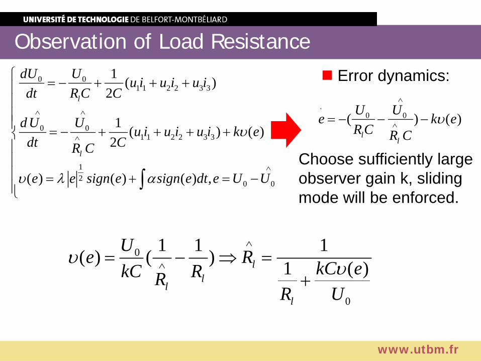
Observation of Load Resistance
www.utbm.fr
Error dynamics:0 01 1 2 2 3 3
0 01 1 2 2 3 3
12
0 0
1 ( )2
1 ( ) ( )2
( ) ( ) ( ) ,
l
l
dU U u i u i u idt R C C
d U U u i u i u i k edt CR C
e e sign e sign e dt e U U
υ
υ λ α
∧ ∧
∧
∧
= − + + + = − + + + + = + = −
∫
0 0( ) ( )l
l
U Ue k eR C R C
υ∧
⋅
∧= − − −
Choose sufficiently large observer gain k, sliding mode will be enforced.
0
0
1 1 1( ) ( ) 1 ( )ll
ll
Ue R kC ekC RRR U
υ υ∧
∧= − ⇒ =+

Power Factor Calculation
www.utbm.fr
1 cos( )h dIPF PF PFI
φ= × = ×
hPF harmonic distortion
φ phase shift between input current and main voltage
1I main current harmonic
I total current RMS
0
1( ( )) ( )T
RMS i t i dT
τ τ= ∫ T is the period of i(t)
Remark: Using Fourier analysis, harmonic distortion measurement, trigonometric modules in matlab, the power factor of the system can easily be obtained.
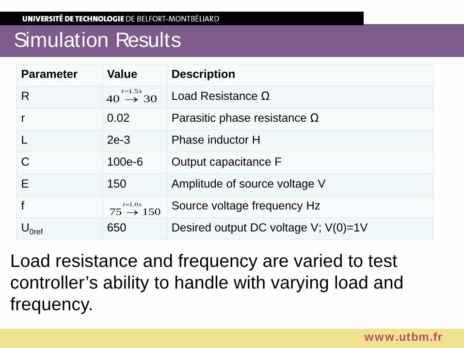
Simulation Results
www.utbm.fr
Parameter Value Description
R Load Resistance Ω
r 0.02 Parasitic phase resistance Ω
L 2e-3 Phase inductor H
C 100e-6 Output capacitance F
E 150 Amplitude of source voltage V
f Source voltage frequency Hz
U0ref 650 Desired output DC voltage V; V(0)=1V
1.540 30
t s=
→
1.075 150
t s=
→
Load resistance and frequency are varied to test controller’s ability to handle with varying load and frequency.
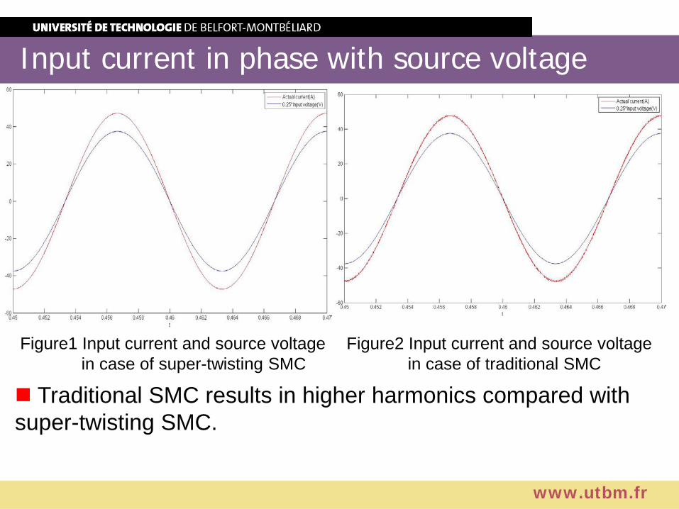
www.utbm.fr
Figure1 Input current and source voltagein case of super-twisting SMC
Traditional SMC results in higher harmonics compared with super-twisting SMC.
Figure2 Input current and source voltagein case of traditional SMC
Input current in phase with source voltage

www.utbm.fr
Figure3 Source voltage Ug1 estimation within the windows when ilink is equal to i1
Source voltage can be reconstructed with super-twisting observer without designing a low-pass filter.
Source Voltage Estimation

www.utbm.fr
Figure4 Load resistance R estimator performance
Figure4 shows the performance of load resistance estimation.
Load Resistance Estimation

www.utbm.fr
Figure5 Output voltage estimatorperformance
Figure6 Current estimator performance0U
∧qi
∧
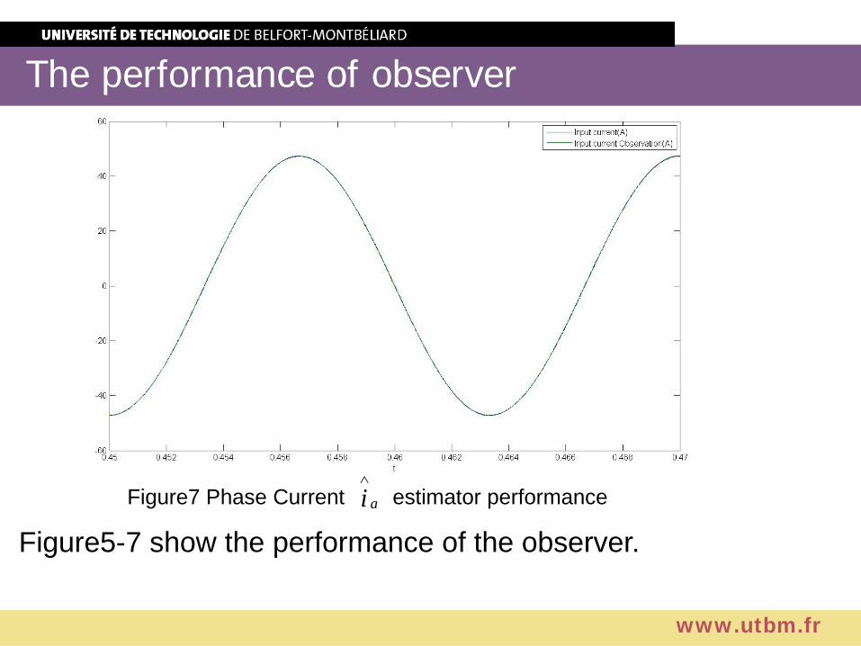
The performance of observer
www.utbm.fr
Figure5-7 show the performance of the observer.Figure7 Phase Current estimator performanceai
∧
The performance of observer
www.utbm.fr
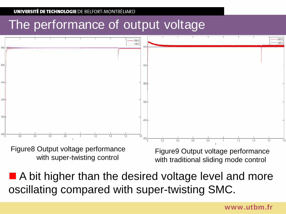
Figure8 Output voltage performance with super-twisting control
A bit higher than the desired voltage level and more oscillating compared with super-twisting SMC.
Figure9 Output voltage performance with traditional sliding mode control
The performance of output voltage

www.utbm.fr
Figure10 Power factor with super-twisting control
Less value and more oscillations compared with super-twisting control. The super-twisting control was able to produce a power factor that was more than 99%, and can withstand the changing conditions.
Figure11 Power factor with Traditional SMC
Power Factor
Conclusions
www.utbm.fr
The proposed control method can achieve a power factor close to unity.
Power Balance Condition is taken into account to achieve the desired performance of the system.
The proposed super-twisting observer demonstrates its robustness to the change in operational conditions.
Source Voltage Estimation is achieved with ilink via super-twisting method without using low-pass filter.

Thanks!If you have any questions, I would be pleased to answer them!
www.utbm.fr


