Oskar Norald Nyheim Solbraekke
Cross-country differences in returns to capital in the oil and gas industry
Dissertação de Mestrado
Dissertation presented to the Programa de Pós-graduação em Macroeconomia e Finanças of the Departamento de Economia, PUC-Rio, in partial fulfillment of the requirements for the degree of Mestre em Macroeconomia e Finanças.
Advisor: Prof. Pablo Salgado
Co-advisor: Prof. Arthur Bragança
Rio de Janeiro April 2018
PUC
-Rio
-Cer
tific
ação
Dig
italN
º151
3677
/CA

Oskar Norald Nyheim Solbraekke
Cross country differences in returns to capital in the oil and gas industry
Dissertation presented to the Programa de Pós-Graduação em Macroeconomia e Finanças of the Departamento de Economia, PUC-Rio as a partial fulfillment of the requirements for the degree of Mestre em Macroeconomia e Finanças. Approved by the following comission:
Prof. Pablo Salgado Advisor
Departamento de Economia – PUC-Rio
Prof. Arthur Bragança Co-Advisor
Departamento de Economia – PUC-Rio
Prof. Marcelo Medeiros Departamento de Economia – PUC-Rio
Prof. Fernando Roriz Ventor Investimentos
Prof. Augusto Cesar Pinheirto da Silva Vice Dean of Graduate Studies
Centro de Ciências Sociais – PUC-Rio
Rio de Janeiro, April 20th, 2018.
PU
C-R
io-C
ertif
icaç
ãoD
igita
lNº1
5136
77/C
A
All rights reserved.
Oskar Norald Nyheim Solbraekke
Economics graduate from PUC-Rio in 2014, with the bachelor thesis about the natural resource curse and with a Master in economics at PUC-Rio concluded in 2018. Currently working at Scatec Solar in Oslo, Norway.
Bibliographic data
CDD: 330
Solbraekke, Oskar Norald Nyheim Cross-country differences in returns to capital in the oil and gas industry / Oskar Norald Nyheim Solbraekke ; advisor: Pablo Salgado; co-advisor: Arthur Bragança. – 2018. 58 f. ; 30 cm Dissertação (mestrado) – Pontifícia Universidade Católica do Rio de Janeiro, Departamento de Economia, 2018. Inclui bibliografia 1. Economia – Teses. 2. Fluxos de capital. 3. Paradoxo de Lucas. 4. Desenvolvimento econômico. 5. Economia de petróleo e gás. 6. Instituições. I. Seuanez Salgado, Pablo Hector. II. Bragança, Arthur Amorim. III. Pontifícia Universidade Católica do Rio de Janeiro. Departamento de Economia. IV. Título.
PU
C-R
io-C
ertif
icaç
ãoD
igita
lNº1
5136
77/C
A

Abstract
Solbraekke, Oskar Norald Nyheim; Salgado, Pablo (Advisor); Bragança, Arthur (Co-advisor). Cross country differences in returns to capital in the oil and gas industry. Rio de Janeiro, 2018. 58p. Dissertação de Mestrado, Departamento de Economia, Pontifícia Universidade Católica do Rio de Janeiro.
This thesis makes use of a unique and vast dataset of investment and
production in the oil and gas industry from 1950 to 2016, to explore the Lucas
Paradox and the drivers of returns to capital in the industry. Firstly, the thesis
examines to what extent poor countries possess higher average returns to capital
than rich countries. Secondly, it investigates whether the differences in returns
between countries are correlated with institutional factors, variance and/or
asymmetry in the returns. The results demonstrate that poorer countries have
enjoyed significantly higher returns to capital than richer countries. Moreover, the
findings show that institutional factors such as property rights protection, level of
corruption and level of schooling possess a positive and statistically significant
correlation with returns to capital. However, both these findings are not
particularly economically significant. Variance and asymmetry of the returns
appear to be an irrelevant explanation for the Lucas Paradox. On the other hand,
asset-specific factors, that were, ex-ante, expected to be merely insignificant
control variables, such as the size of the reservoir, or whether the asset is located
onshore or offshore, have large R-squared impact on returns to capital. The
findings in this thesis are important because the largely insignificant magnitude of
country-specific variables highlight the importance of adapting economic
development theory to account for sector-specific differences, as emphasized by
Feyrer and Caselli (2008). Moreover, the results indicate that profit maximizing oil
and gas companies considering new investments in a country should not be overly
concerned with the GDP per capita nor the institutional quality of the country in
question. Several potential explanations and paths for future studies are delineated.
Keywords
Capital flows; Lucas paradox; Development economics; Oil and gas economics; Institutions.
PU
C-R
io-C
ertif
icaç
ãoD
igita
lNº1
5136
77/C
A

Resumo
Solbraekke, Oskar Norald Nyheim; Salgado, Pablo (Advisor); Bragança, Arthur (Co-advisor). Diferenças de retornos de capital entre países na indústria de petróleo e gás. Rio de Janeiro, 2018. 58p. Dissertação de Mestrado, Departamento de Economia, Pontifícia Universidade Católica do Rio de Janeiro.
Primeiramente, o trabalho examina em que medida os países pobres
possuem retornos de capital mais elevados que os países ricos. Em segundo lugar,
investiga se as diferenças nos retornos de capital entre países estão
correlacionadas com fatores institucionais, variância e/ou assimetria nos retornos.
Os resultados indicam uma relação negativa entre os retornos e o PIB per capita
mas com pouca significância econômica. Ademais, os resultados indicam
correlações significantes entre retornos de capital e alguns fatores institucionais,
embora esses também não sejam economicamente significativos. O desvio padrão
ou a assimetria nos retornos não parecem estar correlacionados com os retornos.
Em suma, os achados indicam que uma pior qualidade institucional é, até certo
ponto, uma explicação plausível para altos retornos de capital nos países pobres.
Ainda assim, a falta de significância econômica encontrada destaca a natureza
idiossincrática dos retornos nesta indústria devido a independência entre retornos
e fatores específicos ao país. Os resultados indicam a necessidade de adaptar a
teoria economia à differenças setoriais e também é importante na prática para
empresas privadas no setor de petróleo e gás, pois os resultados indicam que estas
não devem se preocupar particularmente com o PIB per capita ou as instituições
dos países em que considera investir. Ao invés disso, os resultados indicam que as
empresas devem olhar principalmente para características dos poços mesmo.
Diversas explicações plausíveis para os resultados são delineadas.
Palavras-chave
Fluxos de capital; Paradoxo de Lucas; Desenvolvimento econômico; Economia de Petróleo e Gás; Instituições.
PU
C-R
io-C
ertif
icaç
ãoD
igita
lNº1
5136
77/C
A

Table of contents
1 Introduction 7
2 The Data 12
2.1 The Rystad Energy Database 12 2.2 The Sample 12 2.3 Description of variables 13 2.4 The lifecycle of oil and gas assets 18
3 Method 21
3.1 Creating measures of return to capital 21 3.1.2 “Return lifecycle” 21 3.1.3 “Return twenty” 22 3.2 Multivariate regression: What explains the returns to capital during the lifecycle of oil and gas assets? 23 3.3 Robustness Exercise: Testing one institutional factor at a time 27 3.4 Robustness Exercise II: Testing different measures of returns 32 3.5 Robustness Exercise III: Running the regressions without government take 35 3.6 Robustness Exercise IV: Running the regressions with different institutional variables 36 3.7 Relationship between average returns to capital and variance and assymetry of returns 38
4 Discussion of results 41
4.1 Discussion of results 41 4.2 Limitations and assumptions 42
5 Conclusion 44
6 References 45
7 Appendix 47
PU
C-R
io-C
ertif
icaç
ãoD
igita
lNº1
5136
77/C
A
1 Introduction
In 1990, Robert Lucas raised an important and puzzling question: Why does
capital not flow from rich to poor countries?1 According to Lucas’ argument, the
traditional Solow framework implies the marginal product of capital should be 58
times higher in rich countries than in poor countries to explain the existing
differences in output per worker. Consequently, even when allowing for highly
imperfect capital mobility, these differences would make investing in rich
countries irrational and thus induce vast amounts of capital to move from rich to
poor countries. However, the opposite has been observed empirically. This
apparent economic development puzzle was later coined “the Lucas paradox”.
The Lucas paradox should thus be understood as a criticism of the neoclassical
framework and has become a classic concept in modern development economics.2
Another way of stating the underlying theoretical problem is as follows: Can one
rationalize why capital does not flow from rich countries to poor countries despite
the fact that poor countries exhibit higher marginal returns to capital? And, if it
may indeed be rationalized, what are the most important factors impeding such
capital flows? This thesis makes use of a unique, extensive and complete cross-
country panel dataset of cash-flows and production figures for the oil and gas
industry from 1950 to 2016 to examine the following: I) Ceteris paribus, do less
developed countries exhibit higher rates of return to capital than more developed
countries in the oil and gas industry? II) Can institutional quality or variance
and/or asymmetry in returns help explain the return differentials between poor and
rich countries?
A distinct feature making the oil and gas industry attractive for cross-
country comparisons of returns to capital is that it is arguably the most
homogenous industry in the world in terms of inputs and outputs of production.
Both the technology used for production (inputs) and the final product (oil, gas
1 Lucas, Robert. 1990. “Why doesn’t capital flow from rich to poor countries? The American Economic Review, p.92-96. 2 For a summary of the explanations and importance of the Lucas Paradox see Laura Alfaro et al 2008. "Why Doesn't Capital Flow from Rich to Poor Countries? An Empirical Investigation," The Review of Economics and Statistics, MIT Press, vol. 90(2), p.347-368.
PU
C-R
io-C
ertif
icaç
ãoD
igita
lNº1
5136
77/C
A

and other natural liquids) are largely the same worldwide, which permits
“comparing apples with apples”. Moreover, the oil and gas industry is one of the
largest industries in the world and represents a high percentage share of the GDP
of many countries, in particular of developing countries. If one finds that the
returns to capital in the oil and gas industry are substantially higher in poor than in
rich countries, this would indicate a potential presence of the Lucas paradox in
this specific industry.
The results found in this thesis indicate that that poor countries, as measured
by GDP per capita, do not exhibit higher returns to capital (in the oil and gas
sector) than rich countries. Moreover, results indicate that although some country-
specific institutional factors, such as level of corruption, level of schooling,
property rights protection possess a (mostly) robust and (almost always)
statistically significant correlation with returns to capital between 1950 and 2016,
such results are rather economically insignificant, while a myriad of other
intuitional factors that are tested for do not at all correlate with returns to capital.
Instead, other factors related to the characteristics of the assets (namely, the size
of the hydrocarbon reserves and whether the asset is located onshore or offshore)
are, under all specifications, more impactful than any institutional variables.
Lastly, the thesis does not find evidence for any correlation between returns and
variance nor asymmetry of the returns which could potentially help rationalize
return differentials. A plethora of theoretical explanations for the Lucas paradox
have emerged since 1990, but the evidence is not particularly robust and the
explanations lack consensus. Alfaro et al. (2003) categorize the explanations in
two main lines of reasoning: 1) differences in fundamentals affecting the
production structure, such as factors of production, government policies and
quality of institutions, and 2) international capital market imperfections, mainly
sovereign risk and asymmetric information. For each of these two lines of
reasoning, authors have adopted various methodologies to test the validity.
Regarding differences in fundamentals of the production function as an
explanation for the paradox, a popular procedure, performed by Alfaro et al
(2003), Caselli and Feyrer (2008) and Steger and Schularick (2008) for example,
is performed by expanding the basic neoclassical production function so that it
incorporates endowments of complementary factors of production, such as human
PUC
-Rio
-Cer
tific
ação
Dig
italN
º151
3677
/CA

capital. Subsequently, a calibration exercise for the expanded model is performed
and tested against a given dataset.
One would expect poor countries to exhibit higher rates of return to capital
simply because of the scarcity of capital per worker. Nonetheless, while factors
such as human capital and low total factor productivity (TFP) decreases the
marginal product of capital, bad government policies and low institutional quality
increases its inherent risk since the marginal product of capital becomes more
volatile. For instance, Besly (1995) provide convincing empirical evidence to
support the view that poor property right protection has significantly lowered rates
of investment in Ghana. As such, bad government policies (e.g. rent-seeking
behavior or expropriation) and low institutional quality may be viewed as factors
of production omitted by the neoclassical production function and, thus, as
components representing risk for investors. Following this line of reasoning, a
large return to capital disparity between poor and rich countries may be
rationalized by the fact that investors require higher expected returns to
compensate for the additional risk incurred by investing in poor countries. In other
words, it is possible that the expected risk-adjusted returns to capital are actually
quite similar across countries and that therefore there is no Lucas paradox.
Similar cross-country risk-adjusted returns to capital is often referred to as
“return equalization”. Alfaro et al. (2003) attempts to directly measure the
determinants of capital inflows through cross-country regressions to “solve” the
paradox. Their results showed that for the period 1971–1998, institutional quality
is the most important and causal explanatory factor determining capital flows,
while capital market imperfections, or market failures, play a role but are less
economically significant. Furthermore, the authors point to the fact that
international capital market failures cannot be an explanation for the lack of flows
before 1945 since “during that time, the entire so-called third world was subject to
European legal arrangements imposed through colonialism,” meaning that the gap
in institutional quality between poor and rich countries was negligible pre-WWII,
but lack of capital flows was still occurring. A fundamental assumption for the
return equalization approach is that under conditions approximating perfect
competition in the global capital market, the marginal productivity to capital is
equal to the rate of return to capital.
PUC
-Rio
-Cer
tific
ação
Dig
italN
º151
3677
/CA

Steger and Schularick (2008) extend Lucas’s original model to account for
the impact institutional quality has on differentials of returns. The authors argue
that the gap in institutional quality between poor and rich countries was much
narrower before WWII because the legal and economic arrangements of private
contracts were most of the time directly imposed by European powers, an effect
often referred to as the “empire effect.” Thus, they argue, the fact that flows of
capital from rich to poor countries have decreased substantially between 1914 and
today can be rationalized by the fact that the institutional gap, specifically
property rights, has also substantially increased. An equivalent way of looking at
it is that sovereign-risk in emerging markets is relatively higher today than in
1914, which may explain why capital flows from rich to poor countries have
decreased. Hence, Steger and Schularick (2008) and Alfaro et al. (2003) agree that
institutional quality is a paramount explanation for the paradox.
Caselli and Feyrer (2007) also analyzes the Lucas Paradox through
analyzing differences in fundamentals of the production function, but they
estimate the marginal returns to capital, instead of capital flows determinants as
the aforementioned authors. They find that the marginal return to capital is
remarkably similar across countries when explicitly adjusting the neoclassical
model to account for the higher relative price of capital in poor countries than in
rich countries and, simultaneously, distinguishing between reproducible rates of
capital and non-reproducible rates of capital. The authors argue that standard
measures of returns to capital use a capital share that is inappropriate because it
conflates the incoming flowing to capital accumulated through investment flows
with natural capital in the form of land and natural resources. Together, the two
abovementioned facts are enough for returns to capital to be essentially equalized
between the countries in their sample, which they argue means that one may
rationalize all the cross-country variation in returns to capital without appealing to
credit-market imperfections. Hence, according to these authors, there is no
support for the view that international credit frictions play a major role in
preventing capital flows from rich to poor countries.
The second main line of academic papers examines the credit market
imperfection explanation for the Lucas paradox by measuring specific hypotheses
through microeconomic data and natural experiments. Notably, Udry and Anagol
PUC
-Rio
-Cer
tific
ação
Dig
italN
º151
3677
/CA

(2006) calculate the returns to capital in Ghana’s agricultural sector. They show
that the real return to capital in Ghana’s informal sector is high. For farmers, they
find annual returns ranging from 205–350% in the new technology of pineapple
cultivation which is more informal and generally has less access to credit than
other agricultural activities, and 30– 50% in well-established food crop
cultivation. A more recent paper by David, Henriksen and Simonovska (2014)
finds that poor and emerging markets do, in fact, present higher average returns to
capital than rich countries through panel-regressions of a set of 144 countries
between 1950 and 2011. However, crucially, the authors document that capital
does not flow to poor countries until returns are equalized precisely because these
countries represent the riskiest investments. More specifically, the authors
document a strong correlation between the countries’ expected returns and the
beta of US stocks. “Countries that have high returns tend to have a high beta with
US returns”, they conclude. Both of these papers may be used as evidence to
support the view that credit market imperfections are indeed a significant
explanation for the Lucas Paradox.
Lastly, although not directly motivated by the Lucas Paradox, Hsieh and
Klenow (2008) examine the source of resource misallocation and its negative
effects on total factor productivity. The authors provide evidence that the variance
and skewness of the marginal products of labor and capital in India and China is
much higher than in the US. They then proceed to show that if the marginal
products to capital and labor were as efficiently (more evenly distributed, that is)
allocated as in the US, India and China could experience an increase between 30–
60% in total factor productivity. This is a different branch of research, but
nevertheless relevant to this thesis because high returns to capital in poor
countries could be potentially be correlated with high variance or asymmetry in
returns and thus serve as a potential underlying explanation for returns
differentials. Nonetheless, the empirical evidence presented herein does not
support standard deviation or asymmetry as possible explanations for the Lucas
paradox.
PUC
-Rio
-Cer
tific
ação
Dig
italN
º151
3677
/CA

2 The Data 2.1 The Rystad Energy Database
The database from which the sample originates is owned by Rystad Energy,
a Norwegian-based consultancy and business intelligence firm used by investment
banks, governments and universities around the world. Rystad Energy owns
several databases, but only their “UCube” (an abbreviation for Upstream Cube) is
used in this study. The UCube includes historical production and economic
figures for about 65,000 oil and gas upstream assets and 3,200 operators in 70
countries3. The economic figures encompass capital expenditure, operational
expenditure and government take4 between 1900 and 2016. Furthermore, the
economic and production data per asset are classified by whether they are located
onshore or offshore and by country and operator. Assets located offshore are
further broken down by categories of water depth.5
2.2 The sample
For the purpose of answering the questions proposed, several important
restrictions were applied to the data. A subset of 29 countries was chosen from a
total of 70 countries in the original database. The countries were selected
according to a few criteria. First, assets within countries with the largest volume
of oil and gas production in 2016 were selected. Second, only assets with a total
sum of economics (capex + opex + government take) exceeding 20 million
nominal USD over the lifecycle6 of the asset were included. The rationale behind
these exclusions is that oilfields with very small total cost are more prone to
measurement error due to their small magnitudes and because these small assets
3 Upstream is usually defined as a synonym of the exploration and production (E&P). However, to avoid confusions with midstream and downstream phases, perhaps “exploration and extraction of hydrocarbons” would be a more precise description of the term. Assets are synonymous of oil and gas fields. Operators are firms responsible for operations on the oilfield. See section 2.4 for details 4 Or received, in the case of negative values for government take. See section 2.4. 5 See section 2.4 for more detailed descriptions. 6 See explanation and details about lifecycle in section 2.3.
PU
C-R
io-C
ertif
icaç
ãoD
igita
lNº1
5136
77/C
A

are less closely followed by Rystad. Furthermore, estimating the average rate of
return to capital within a country with very few and economically insignificant
assets could potentially lead to miscomputing the variance and asymmetry of
returns within that country. There is no reason to believe that this exclusion
should lead to any systemic bias in the calculations, even though a large sample of
countries could of course have increased the precision cross-country regressions.
Lastly, observations before 1950 were excluded due to the presence of outliers
and incomplete observations.
2.3 Description of variables
A short explanation of each of the relevant variables in my analysis is in
order here, as follows:
ASSET
Asset refers to the name of a specific oil and gas field. Originally, the total
number of assets was 10,524 assets. After making relevant exclusions, such as
deleting assets for which no capex was listed and restricting the years of the
sample to only 1950–2016, a total of 10,194 assets were included in the final
dataset. I also used the same dataset but restricted to the interval 1996-2016 to
check for correlations with a second dataset for institutional quality that was only
available for 1996 to 2016.
COUNTRY
Naturally, the country variable refers to the country in which the asset is
physically located. The countries included are selected on the basis of being the
largest oil producing countries in 2016. It is important that the countries included
have a significant amount of oil and gas assets because of the increased precision
of my variance estimates later on. See Table A for an overview of countries and
the number of assets in each country.
PUC
-Rio
-Cer
tific
ação
Dig
italN
º151
3677
/CA

Table A: Number of assets and the income classification of the world bank by country
COUNTRY Country Code Number of assets Income
classification
United Arab Emirates AE
42 High income
Angola AO 83 Lower middle
income
Argentina AR 376 Upper middle
income
Australia AU 427 Upper middle
income
Azerbaijan AZ 40 Upper middle
income
Brazil BR 200 Lower middle
income
Chile CL 57 Upper middle
income
China CN 464 Lower middle
income
Congo CO 392 Low income
Denmark DK 17 High income
Algeria DZ 115 Lower middle
income
Egypt EG 20 Lower middle
income
Great Britain GB 306 Upper middle
income
Indonesia ID 493 Lower middle
income
India IN 228 Lower middle
income
Iraq IQ 56 Upper middle
income
Iran IR 91 Upper middle
income
Kuwait KW 11 High income
Libya LY 114 Lower middle
income
Mexico MX 313 Upper middle
income
Malaysia MY 290 Low income
Nigeria NG 244 Low income
Norway NO 86 High income
Qatar QA 24 High income
PUC
-Rio
-Cer
tific
ação
Dig
italN
º151
3677
/CA

Saudi Arabia SA 34 High income
Venezuela VE 211 Lower middle
income
Canada CA 1492 Upper middle
income
Russia RU 1558 Upper middle
income
United States US 2142 High income
OPERATIONAL EXPENDITURE
Opex includes all operational expenses directly related to the oil and gas
activities of an asset. Included items are production costs (i.e., salaries, lease costs
and maintenance work), transport costs (processing costs and transport fees) and
general and administrative costs. Negative values for opex should not occur and
assets with such values were thus excluded in the final sample.
CAPITAL EXPENDITURE
Capex includes investment costs incurred related to the development of
infrastructure, drilling and the completion of wells, as well as modifications and
maintenance on installed infrastructures. It is important to note that this measure
captures only the capital expenditure related to a specific oil field. Any capital
expenditure spent by the operator on non-field-specific costs is not accounted for.
On the other side, as most operators in the oil and gas supply-chain operate in
several countries, there is little reason to believe this would create any type of
systemic bias in my returns of capital estimates. Additionally, neither of my cost
measures explicitly captures the exploration costs (costs related to encountering,
evaluating and appraising the oil and gas fields) because this figure was not
available. This creates a potential bias for my estimates of the real rate of return to
capital because it is possible that some countries possess geological conditions
that would make finding and appraising fields much costlier on average than in
other countries. Controlling for whether the asset is located onshore or offshore
should attenuate this problem, but there is no guarantee it resolves it entirely.
GOVERNMENT TAKE
Government take includes not only all cash flows destined for authorities
and governments but also rent payments to private land owners (particularly
PUC
-Rio
-Cer
tific
ação
Dig
italN
º151
3677
/CA

relevant for the US), export duties, bonuses, income taxes and all other taxes and
fees. Government take is the only one of my variables that includes negative
values. Negative values for government take represent payments from authorities
to the operators in the form of subsidies.
PRODUCTION
Production is the total amount of barrels of oil equivalents (BOE) produced
from an asset. BOE is a form of combining and incorporating the production of
natural gas and other liquids into an energy measure equivalent to that of oil and
gas. Some imprecision is introduced through using BOE as a measure of
production since the monetary value of natural gas is somewhat lower than crude
oil. It is possible that this imprecision may lead to minor bias in the data if some
countries possess much higher proportions of low quality liquids and natural gas,
but this is not likely to yield major differences.
REVENUE
Revenue is simply equal to the production in a given year multiplied by the
oil price in the corresponding year. The oil price utilized in the calculations is an
average of the Brent and WTI prices. Revenue is given in nominal USD.
ONSHORE VS. OFFSHORE
This variable is a dummy variable, taking on the value 1 if the asset is
located offshore (that is, at sea) and 0 if the asset is located onshore (that is, on
land). It is important to make this distinction because one would expect that capex
and opex are generally higher for assets located in the water due to geological and
logistical challenges.
WATER DEPTH CATEGORY
Water depth splits the assets into categories of different water depth. The
“depth” is a measure of the distance between the facility (platform, FPSO, etc.)
and the wellbore. In general, a lengthier distance implies greater operational and
capital expenditure due to the logistical and geological challenges. For very deep
water depths, such as the pre-salt region in Brazil, the operator will have to drill
PUC
-Rio
-Cer
tific
ação
Dig
italN
º151
3677
/CA

through thousands of meters of water, salt and various rock formations, which
makes production in these areas costlier. The intervals of the categories are 25
meters up to 200 meters, and hence the intervals increase with the water depth.
This variable is thus an important control variable in the methodology because it
serves as a control for geological difficulties in extracting the hydrocarbons.
Unfortunately, this variable is the sole control variable for geological challenges
in my regressions. Ideally, one would also control for variables that relate more
directly to the geological and geophysical particularities of the reservoirs in each
asset (such as the type of rock formation, porosity, permeability, pressure, etc.).
Unfortunately, figures for such characteristics were not available in the database.
On the other hand, there is little reason to believe that this omission would lead to
a systemic bias when measuring differences of returns to capital between poor and
rich countries. Instead, it likely represents a source of imprecision of unknown
magnitude.
INSTITUTIONAL MEASURES
As earlier described, one would expect countries with poorer institutional
quality to display higher marginal return. To measure the role of institutional
quality, I run my three distinct measures of returns to capital against two different
datasets of institutional quality. The first regressions rely on data derived from the
World Governance Indicators (WGIs) by the World Bank. These measures range
between 1996 and 2016 and include four distinct measures of institutional quality:
control of corruption, government effectiveness, political stability and absence of
violence/terrorism and regulatory quality. The measures of the institutional quality
in each country are derived from the World Bank’s governance indicators. The
Worldwide Governance Indicators (WGI) cover over 200 countries and territories,
measuring six dimensions of governance starting in 1996. Voice and
Accountability, Political Stability and Absence of Violence/Terrorism,
Government Effectiveness, Regulatory Quality, Rule of Law and Control of
Corruption. Political stability and absence of violence/terrorism measures
perceptions of the likelihood of political instability and/or politically motivated
violence, including terrorism. Regulatory quality captures perceptions of the
ability of the government to formulate and implement sound policies and
PUC
-Rio
-Cer
tific
ação
Dig
italN
º151
3677
/CA

regulations that permit and promote private sector development. Control of
corruption captures perceptions of the extent to which public power is exercised
for private gain, including both petty and grand forms of corruption as well as the
“capture” of the state by elites and private interests.7 Government effectiveness
captures perceptions of the quality of public services, the quality of the civil
service and the degree of its independence from political pressures, the quality of
policy formulation and implementation and the credibility of the government’s
commitment to such policies.
A second source for institutional measures is derived from the “Quality of
Government” database provided by Oxford University Press in 1999. Differently
than the above-mentioned dataset, this dataset is not longitudinal but only cross-
section. One may argue, nevertheless, that this is not a problem for the precision
of the results given the slow-paced change of measures of institutional quality.
GDP PER CAPITA
As the research question clearly stated, the first objective of this thesis is to
verify whether poor countries exhibit higher returns to capital than rich countries
in the oil and gas industry. The results, summarized in tables I-VIII indicate, as
expected, that low income countries do possess higher returns to capital than high
income countries in my sample, although the effect is generally quite small in
terms of magnitude. As previously mentioned, one would expect, based on
previous academic findings, a negative correlation between GDP per capita and
returns to capital in the oil and gas sector. The GDP per capita measures provided
by the Institute for Health Metrics and Evaluation have been used in this thesis
because they contain complete data for all countries in the sample and between
years 1950 and 2016.
2.4 The lifecycle of oil and gas assets
It is important to elaborate and clarify what is meant by the lifecycle of an
oil and gas asset to understand how many years are included in the calculation of
the returns to capital and thus better understand the data. Lifecycle refers to the 7 https://info.worldbank.org/governance/wgi/pdf/cc.pdf
PUC
-Rio
-Cer
tific
ação
Dig
italN
º151
3677
/CA

lifespan of the field divided into distinct phases. Some of the phases may overlap
and possess more detailed information, but this summary should nonetheless
suffice for the purpose of this exercise. Below I present these phases in a
stereotypical, simplistic and summarized manner.
PHASE 1 – LICENSING
Licensing consists of screening and identifying prospective areas to explore.
Then the operator acquires leased acreage from the government, typically in
exchange for a fee and some form of performance or work obligation, such as the
acquisition of seismic data or drilling a well.
PHASE 2 – SEISMIC, SURVEYS AND EXPLORATION DRILLING (3–5 YEARS)
Seismic, and sometimes magnetic and electromagnetic, surveys are
developed to understand the geology below the surface. If the results indicate the
existence of potential hydrocarbon reservoirs, the oil and gas company, or
operator, may continue with site surveys. The site surveys are performed to gain
more information on the prospect area. Next, the operator can drill one or more
exploration wells to gather further data to evaluate whether the well is viable for
production. This includes information such as flow rates, pressures and
temperatures.
PHASE 3 – APPRAISAL (4–10 YEARS)
If substantial hydrocarbon reservoirs are confirmed, a field appraisal is used
to determine the methodology of extraction and whether the field is indeed
economically viable.
PHASE 4 – DEVELOPMENT (1–7 YEARS)
After a prospect has been judged commercially and technically viable, a
development plan is submitted to the authorities, and necessary goods and
services are procured. Production wells are then drilled, followed by the
commissioning of the area to attain a stable production level.
PUC
-Rio
-Cer
tific
ação
Dig
italN
º151
3677
/CA

PHASE 5 – PRODUCTION (10–30 YEARS)
There is a large variety of alternatives for how an oil and gas asset will
produce, depending on the type of field (onshore vs. offshore, deep water vs.
shallow water, pre vs. post salt, etc.), the country and environmental conditions.
Production is generally gradually increased to peak production, the level at which
the asset will produce at plateau level for some time. At some point, the
production starts to decline due to falling pressure, at which point the operator
may inject water or gas to maintain the pressure or, alternatively, use techniques
such as infill drilling to connect nearby reservoirs to the developed facility.
As previously mentioned, the very concept of life cycles in the reason why I
have chosen to include future projections for production, capex and opex. The
database provider I have used can easily deliver unbiased, albeit not necessarily
exact, estimates for the remaining life cycles of an oil and gas asset. For example,
if an asset has been explored, appraised and produced for one year up until 2016,
Rystad Energy knows, with a high degree of certainty, that more oil and gas will
be produced. If this future production is not accounted for, the returns to capital
for countries with many such assets will be unrealistically penalized. In other
words, a cutoff in year 2016 would create a bias for countries with a large number
of assets that are in the later stages of production. Of course, cost projections are
also included. The scenario used for projecting the cost values (Opex and
Government take) is based on the taxation and subsidy regimes per 2016. Such
cost projections are subject to changes in government policy, for example changes
in taxation, which would alter government take in the future and hence this is a
source of potential measurement errors. Nevertheless, there is little reason to
believe there are any systematic differences between poor and rich countries with
this regard. All this means that we can effectively and fairly compare assets in
different countries. To put it even more informally, the concept of lifecycles
allows us not only to compare apples to other apples, but whole apples to whole
apples. Lastly, in table A you may see descriptive statistics showing the countries
included, number of assets, income classification to give on overview of which
countries are included in the study.
PUC
-Rio
-Cer
tific
ação
Dig
italN
º151
3677
/CA
3 Method 3.1 Creating measures of return to capital
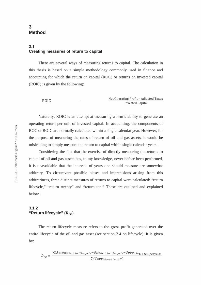
There are several ways of measuring returns to capital. The calculation in
this thesis is based on a simple methodology commonly used in finance and
accounting for which the return on capital (ROC) or returns on invested capital
(ROIC) is given by the following:
=
Naturally, ROIC is an attempt at measuring a firm’s ability to generate an
operating return per unit of invested capital. In accounting, the components of
ROC or ROIC are normally calculated within a single calendar year. However, for
the purpose of measuring the rates of return of oil and gas assets, it would be
misleading to simply measure the return to capital within single calendar years.
Considering the fact that the exercise of directly measuring the returns to
capital of oil and gas assets has, to my knowledge, never before been performed,
it is unavoidable that the intervals of years one should measure are somewhat
arbitrary. To circumvent possible biases and imprecisions arising from this
arbitrariness, three distinct measures of returns to capital were calculated: “return
lifecycle,” “return twenty” and “return ten.” These are outlined and explained
below.
3.1.2 “Return lifecycle” (
The return lifecycle measure refers to the gross profit generated over the
entire lifecycle of the oil and gas asset (see section 2.4 on lifecycle). It is given
by:
=
PU
C-R
io-C
ertif
icaç
ãoD
igita
lNº1
5136
77/C
A

where “t” refers to the time horizon for each variable. The reference point (t = 0)
is the first year of observed production of each particular asset.
The reference point (t = 0) is the first year of observed production of each
particular asset.
“ ” refers to the sum of all operational expenses for an
asset incurred between the first year of production (t = 0) and the last year of
production (lifecycle).
“ ” refers to the sum of all revenue generated for an
asset between the first year of production (t = 0) and the last year of production
(lifecycle).
“ ” refers to the sum of all government take
incurred/received between the first year of production (t = 0) and the last year of
production (lifecycle).
“ ” refers to the sum of all capital expenses for an asset
incurred 10 years before the first year of production (t = -10) and the 10th year of
production (t = 10).
This is the benchmark, or standard, measure of returns to capital on an asset
used in this thesis. It is realistic in the sense that it includes all the observed cash
flows for a particular asset. Thus, it provides a good estimate of how much gross
revenue has been generated per capital expenditure invested. It is important to
note, however, that one potential issue with this measure is that the number of
years of revenue will vary between assets. In other words, the time span between
the first and last year of production is not constant.
3.1.3 “Return twenty” (
The “return twenty” measure is the return in the 20 subsequent years after
the first year of production.
The advantage of this measure compared with “return lifecycle” is that the
PUC
-Rio
-Cer
tific
ação
Dig
italN
º151
3677
/CA

time span between the first and last years of production is always 20 years. The
disadvantage is, naturally, that we are actually not capturing what realistically has
been produced after the first 20 years.
3.1.4 “Return ten” (
The only difference between “return ten” and “return twenty” is the time
span from the first year of production. The advantage of this measure compared
with “return lifecycle” is that the time span between the first and last years of
production is always 10 years. Again, the reason why I chose to create three
different measures of return to capital is simply to increase the robustness of my
findings.
3.2 Multivariate regression: What explains the returns to capital during the lifecycle of oil and gas assets?
The factors affecting returns to capital over the lifecycle of an oil and gas
assets is estimated for a given asset. The benchmark OLS estimation equation is
given by:
(1)
PUC
-Rio
-Cer
tific
ação
Dig
italN
º151
3677
/CA
The dependent variable, , is a logarithmic transformation of “return
lifecycle”. The first independent variable is the level of schooling in 1997 in the
country which each asset is located. Level of schooling is a scale from 1 to 10 and
is a “level variable”, which means that, ceteris paribus, if the level of schooling is
augmented by 1 point, increases by approximately 100 x . The second
independent variable the level of corruption in 1996, which is also measured on a
scale from 1 to 10. The third independent variable is Property rights protection in
1997, again measured on a scale from 1 to 10. All these institutional variables
possess the same above-mentioned interpretation. The fourth independent variable
is a natural log transformation of the Gross Domestic Product per capita in the
country in which the asset is located and in the first year of observed production
of each asset. The interpretation of this result is that a 10% increase in GDP per
capita is associated with a % decrease in . The fifth independent
variable is the log transformation of the total reservoir size of each asset in order
to control for returns to scale effects. The interpretation of this result is that a 10%
rise in the total volume of reserves in the field implies an average of increase of
approximately % in returns to capital. The sixth regressor is a dummy
variable, taking on the value 1 if an asset is located offshore and 0 if the asset is
located onshore. The interpretation is that if an asset is located onshore, is on
average approximately higher than if the asset is located offshore.
The last control variable that is introduced is a fixed year effects in order to
control for economic cycles and technological advancements that may have
occurred in the period from 1950 to 2016.
Table I presents OLS coefficients for specifications in which the
independent variables are gradually introduced. In column 1, three variables
measuring the institutional quality of the variables are introduced without any
additional controls. Both level control of corruption and property rights protection
are both have a positive influence on while, surprisingly “level of schooling”
actually has a strong negative correlation under this specification (as one
introduces more control variables, however, this strange result disappears).
Column 2 introduces the log of GDP per capita as a control variable. As one
would expect, the results show a negative correlation which makes sense
according to the logic of Lucas Paradox; countries with higher GDP per capita,
PUC
-Rio
-Cer
tific
ação
Dig
italN
º151
3677
/CA

should exhibit lower marginal returns to capital. Furthermore, column 3 adds a
fixed-effect for each year in the sample, which increases the R-squared from 0.14
to 0.62. In other words, it is essential to control for economic boom and bust
cycles and the development of relative cost of capital in my sample period. The
same pattern may be recognized in different specifications. In column 4, the log of
the reservoir size as a control variable is introduced, as a manner of controlling for
the returns to scale, since larger assets are expected to yield lower fixed
(operational and capital) costs. This variable has a coefficient of about 0,98,
which means that a 1% increase in reservoir size, leads to a 0,98% rise in .
Lastly, a dummy variable indicating whether a given asset is located onshore or
offshore was introduced as a control variable. The results indicate that onshore
assets exhibit an that is approximately 21,6% higher than offshore assets.
Column 5 is the final benchmark multivariate regression with all controls in place.
The results indicate that an increase in 1 in the index for level of schooling
increases by 32,5%, that a 1 point increase in level of corruption increases
by 9% and that a 1 point increase in property rights protection increases
by 8,7%. In other words, as expected, institutional quality plays a significant
role for returns to capital over the lifecycle of oil and gas assets. Moreover, the
log of GDP per capita in the first year of production of a given asset is negatively
correlated with . An asset located in a country with 10% higher GDP in the
first year of production exhibits an average of approximately 2,31% lower . It
this benchmark regression, all the coefficients are statistically significant at 1%
confidence interval, which is of course mostly a consequence of the sizeable
number of observations.
PUC
-Rio
-Cer
tific
ação
Dig
italN
º151
3677
/CA

Table I: Results are derived from equation (1). The table shows OLS coefficients
with ln of (Return lifecycle) from 1950-2016 as dependent variable. Column
(1) has control of corruption in 1996, level of schooling in 1996 and property
rights in 1997 as independent variables. Column (2) adds the natural logarithm of
GDP per capita in the first year of production as an additional independent
variable. Column (3) adds fixed effects per year as a control variable. Column (4)
adds adds reservoir size, measuring the size of total reserves in the field over its
lifecycle, as a control measure of returns to scale. Column (5) adds the “onshore or
offshore” dummy, as a control for natural given differences. Robust standard errors
are reported in parenthesis. Significance: p<0.01 = ***, p<0.05 = **, p<0.10 = *
Panel A: ln vs Property rights, Corruption and level of schooling under different specifications
(1) (2) (3) (4) (5)
Dependent variable = Level of schooling in 1996 -2.05***
(.138) -0.861***
(.150) -1.107***
(.085) 0.397***
(.055) 0.325***
(.053)
Control of corruption in 1996 0.342*** (.019)
0.501*** (.018)
0.291*** (.0147)
0.091*** (.008)
0.090*** (.008)
Property rights protection 1997 0.543*** (.070)
0.179* (.065)
0.492*** (.038)
0.024*** (.022)
0.087*** (.022)
Log of GDP per capita (first year of production)
-1.113*** (.030)
-0.243*** (.029)
-0.227*** (.023)
-0.231*** (.020)
Log of reservoir size 0.973*** (.011)
0.982*** (.007)
Onshore vs Offshore dummy 0.216*** (.019)
Fixed effects year Yes Yes Yes
0.001 0.14 0.62
0.87
0.88
Number of assets 6539 6539 6488 6488 6488
Average number of assets per country
272 272 270 270 270
Average number of assets per year
99 99 98
98
98
PUC
-Rio
-Cer
tific
ação
Dig
italN
º151
3677
/CA

3.3 Robustness Exercise: Testing one institutional factor at a time
In order to increase the robustness of the findings in section 3.2,
specifications using only one of the institutional variables at the time have also
been tested. The OLS estimation equation for table II, below, is given by:
(2):
When running this multivariate regression (2), with Property Rights
protection being the only institutional variable, the most significant change is that
log of GDP per capita decreases from the benchmark regression (1), even though
the effect is still negative and significant. It is also worth noting that the difference
in average between offshore and onshore shrinks to approximately 14,3%
(compared to 21,6% in table II). The results for regression (2) are summarized in
table II.
The next regression estimated includes control of corruption as the sole
institutional variable, as portrayed in equation (3) below:
(3):
PUC
-Rio
-Cer
tific
ação
Dig
italN
º151
3677
/CA

Under this specification, summarized in table III, the influence of GDP per
capita and onshore vs offshore differential also decreases slightly compared with
(1), while the coefficients for reservoir size and the control of corruption remains
very similar to the benchmark specification.
Lastly, a multivariate regression with level of schooling as the only
institutional variable is estimated, according to the following regression equation:
(4):
The results, summarized in table IV, indicate that level of schooling has
statistically significant and relatively large effect on . The correlation is about
twice as large as the result from the benchmark specification (1). It indicates that
an increase in 1 point in the level of schooling index, leads to an average 75,5%
increase in .
PUC
-Rio
-Cer
tific
ação
Dig
italN
º151
3677
/CA

Table II: Results are derived from equation (2). The table shows OLS
coefficients with ln of (Return lifecycle) from 1950-2016 as dependent
variable. Column (1) has only property rights protection in 1997 as an
independent variable. Column (2) adds the natural logarithm of GDP per capita in
the first year of production. Column (3) adds fixed effects per year as a control
variable. Column (4) adds adds reservoir size which is a category variable
measuring the size of total reserves in the field over its lifecycle, as a control
measure of returns to scale. Column (5) adds the “onshore or offshore” dummy
variable. Robust standard errors are reported in parenthesis. Significance: p<0.01
= ***, p<0.05 = **, p<0.10 = *
Panel A: ln vs Property rights under different specifications
(1) (2) (3) (4) (5)
Dependent variable = Property rights protection 1997 0.052***
(.14) 0.414***
(.02) 0.043** (.015)
0.065*** (.008)
0.077*** (0.009)
Log of GDP per capita (first year of production)
- 0.554*** (.02)
-0.025** (.012)
-0.021*** (.006)
-0.031*** (.006)
Log of reservoir size 1.01*** (.007)
1.006*** (.007)
Onshore vs Offshore dummy 0.143*** (.028)
Fixed effects year Yes Yes Yes
0.02 0.48 0.54
0.88
0.88
Number of assets 9395 9395 9224
9224
9224
Average number of assets per country
319 319 318 318 318
Average number of assets per year
140 140 140 140 140
PUC
-Rio
-Cer
tific
ação
Dig
italN
º151
3677
/CA
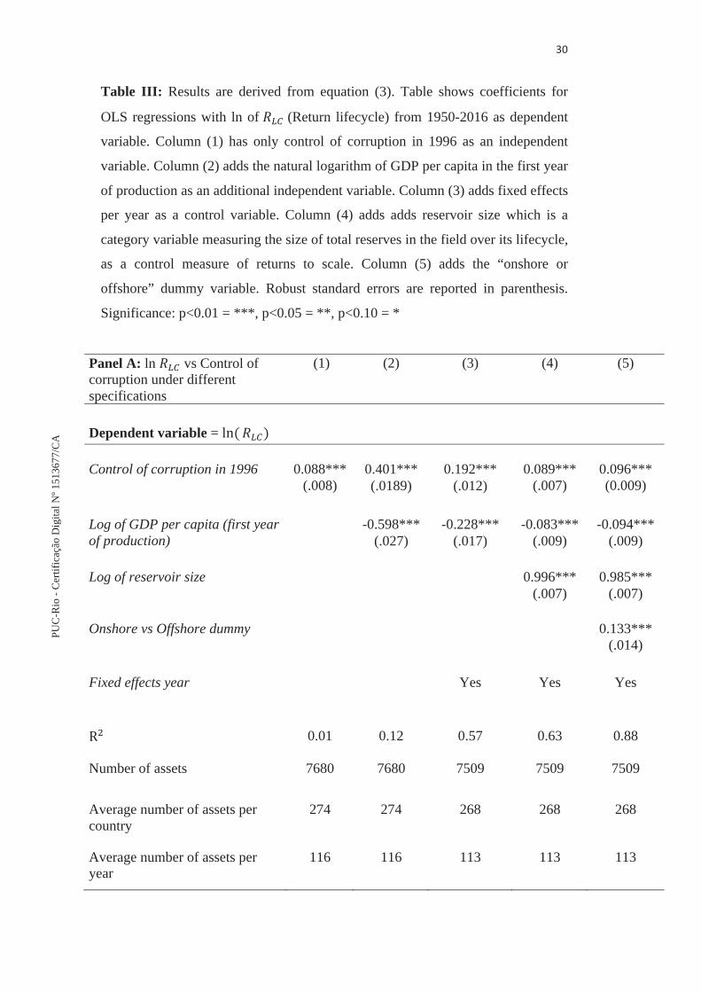
Table III: Results are derived from equation (3). Table shows coefficients for
OLS regressions with ln of (Return lifecycle) from 1950-2016 as dependent
variable. Column (1) has only control of corruption in 1996 as an independent
variable. Column (2) adds the natural logarithm of GDP per capita in the first year
of production as an additional independent variable. Column (3) adds fixed effects
per year as a control variable. Column (4) adds adds reservoir size which is a
category variable measuring the size of total reserves in the field over its lifecycle,
as a control measure of returns to scale. Column (5) adds the “onshore or
offshore” dummy variable. Robust standard errors are reported in parenthesis.
Significance: p<0.01 = ***, p<0.05 = **, p<0.10 = *
Panel A: ln vs Control of corruption under different specifications
(1) (2) (3) (4) (5)
Dependent variable = Control of corruption in 1996 0.088***
(.008) 0.401*** (.0189)
0.192*** (.012)
0.089*** (.007)
0.096*** (0.009)
Log of GDP per capita (first year of production)
-0.598*** (.027)
-0.228*** (.017)
-0.083*** (.009)
-0.094*** (.009)
Log of reservoir size 0.996*** (.007)
0.985*** (.007)
Onshore vs Offshore dummy 0.133*** (.014)
Fixed effects year Yes Yes Yes
0.01 0.12 0.57
0.63
0.88
Number of assets 7680 7680 7509 7509 7509
Average number of assets per country
274 274 268 268 268
Average number of assets per year
116 116 113 113 113
PUC
-Rio
-Cer
tific
ação
Dig
italN
º151
3677
/CA

Table IV Results are derived from equation (4). The table shows OLS
coefficients with ln of (Return lifecycle) from 1950-2016 as dependent
variable. Column (1) has only control of corruption in 1996 as an independent
variable. Column (2) adds the natural logarithm of GDP per capita in the first year
of production as an additional independent variable. Column (3) adds fixed effects
per year as a control variable. Column (4) adds adds reservoir size which is a
category variable measuring the size of total reserves in the field over its lifecycle,
as a control measure of returns to scale. Column (5) adds the “onshore or
offshore” dummy variable. Robust standard errors are reported in parenthesis.
Significance: p<0.01 = ***, p<0.05 = **, p<0.10 = *
Panel A: ln vs Level of schooling under different specifications
(1) (2) (3) (4) (5)
Dependent variable = Level of schooling in 1996 0.278***
(.044) 2.794***
(.123) 0.715***
(.085) 0.711***
(.007) 0.755*** (.0666)
Log of GDP per capita (first year of production)
-.969*** (.041)
- 0.166*** (.017)
-0.196*** (.009)
- 0.203*** (.020)
Log of reservoir size 1.000*** (.010)
0.982*** (.007)
Onshore vs Offshore dummy 0.191*** (.017)
Fixed effects year Yes Yes Yes
0.001 0.14 0.57
0.87
0.88
Number of assets 6539 6539 6488 6488 6488
Average number of assets per country
272 272 270 270 270
Average number of assets per year
99 99 98
98
98
PUC
-Rio
-Cer
tific
ação
Dig
italN
º151
3677
/CA

3.4 Robustness Exercise II: Testing different measures of returns
In this section I emulate the regressions reported in table I with one
important dissimilarity; the dependent variable (that is, the way of measuring
returns to capital). In equation (5) below, the only difference from (1) is that
is substituted for . The results are reported in table V. Similarly, in equation
(6), the only difference from (1) is that is exchanged for . In table V, the
most notable discrepancy from (1) is that “level of schooling” is now both
economically and statistically insignificant. Also, the coefficient for the reservoir
size is considerably smaller than the benchmark, while the difference in return to
capital between onshore and offshore asset is slightly larger than the benchmark
under this specification. In table VI, “level of schooling” is still statistically
significant, but only at 10% level of significance and with a relatively small economic
effect. Other than that, the results only differ slightly in magnitude from table V.
(5)
(6)
PUC
-Rio
-Cer
tific
ação
Dig
italN
º151
3677
/CA

Table V: Results are derived from equation (5). The table shows OLS coefficients
with ln of (Return lifecycle) from 1950-2016 as dependent variable. Column
(1) has control of corruption in 1996, level of schooling in 1996 and property
rights in 1997 as independent variables. Column (2) adds the natural logarithm of
GDP per capita in the first year of production as an additional independent
variable. Column (3) adds fixed effects per year as a control variable. Column (4)
adds adds reservoir size, measuring the size of total reserves in the field over its
lifecycle, as a control measure of returns to scale. Column (5) adds the “onshore or
offshore” dummy, as a control for natural given differences. Robust standard errors
are reported in parenthesis. Significance: p<0.01 = ***, p<0.05 = **, p<0.10 = *
Panel A: ln vs Property rights, Corruption and level of schooling under different specifications
(1) (2) (3) (4) (5)
Dependent variable = Level of schooling in 1996 -1.338***
(.083) -1.779***
(.111) -0.978***
(.099) -0.037 (.072)
0.043 (.072)
Control of corruption in 1996 0.104*** (.012)
0.085*** (.012)
0.136*** (.011)
0.016* (.009)
0.016* (.009)
Property rights protection 1997 0.573*** (.037)
0.641*** (.039)
0.453*** (.035)
0.171*** (.028)
0.104*** (.030)
Log of GDP per capita (first year of production)
0.156*** (.021)
-0.096*** (.029)
-0.093*** (.023)
-0.094*** (.020)
Log of reservoir size 0.599*** (.011)
0.625*** (.016)
Onshore vs Offshore dummy 0.227*** (.023)
Fixed effects year Yes Yes Yes
0.05 0.06 0.25
0.52
0.52
Number of assets 6809 6809 6809 6809 6809
Average number of assets per country
235 235 235 235 235
Average number of assets per year
105 105 105 105 105
PUC
-Rio
-Cer
tific
ação
Dig
italN
º151
3677
/CA

Table VI: Results are derived from equation (6). The table shows OLS
coefficients with ln of (Return lifecycle) from 1950-2016 as dependent
variable. Column (1) has control of corruption in 1996, level of schooling in 1996
and property rights in 1997 as independent variables. Column (2) adds the natural
logarithm of GDP per capita in the first year of production as an additional
independent variable. Column (3) adds fixed effects per year as a control variable.
Column (4) adds adds reservoir size, measuring the size of total reserves in the field
over its lifecycle, as a control measure of returns to scale. Column (5) adds the “onshore
or offshore” dummy, as a control for natural given differences. Robust standard errors
are reported in parenthesis. Significance: p<0.01 = ***, p<0.05 = **, p<0.10 = *
Panel A: ln vs Property rights, Corruption and level of schooling under different specifications
(1) (2) (3) (4) (5)
Dependent variable = Level of schooling in 1996 -1.608***
(.088) -1.191***
(.109) -0.996***
(.108) 0.077 (.079)
0.139* (.079)
Control of corruption in 1996 0.170*** (.013)
0.195*** (.013)
0.196*** (.013)
0.048*** (.008)
0.049*** (.011)
Property rights protection 1997 0.566*** (.041)
0.525* (.042)
0.440*** (.040)
0.096** (.032)
0.044** (.0335)
Log of GDP per capita (first year of production)
-0.166*** (.024)
-0.172*** (.026)
-0.150*** (.022)
-0.147*** (.023)
Log of reservoir size 0.715*** (.014)
0.735*** (.007)
Onshore vs Offshore dummy 0.176*** (.025)
Fixed effects year Yes Yes Yes
0.001 0.14 0.19
0.50
0.51
Number of assets 6621 6621 6621 6621 6621
Average number of assets per country
228 228 228 228 228
Average number of assets p. year 102 102 102 102 102
PUC
-Rio
-Cer
tific
ação
Dig
italN
º151
3677
/CA

3.5 Robustness Exercise III: Running the regressions without government take
In this section I re-run regression (1) except one important distinction; I
exclude government take from the numerator. Thus, the dependent variable
becomes simply:
The reasoning behind this exclusion is that “government take” has a much
more exogenous nature than the other cost variables and is a result of policy, not
productivity. Either way, the results change only slightly from the benchmark
regressions, which is due to the small portion government take represent of the
total fraction.
Table VII: Results are derived from equation (1). The table shows OLS
coefficients with ln of (Return lifecycle – without government take) from
1950-2016 as dependent variable. Column (1) has control of corruption in 1996,
level of schooling in 1996 and property rights in 1997 as independent variables.
Column (2) adds the natural logarithm of GDP per capita in the first year of
production as an additional independent variable. Column (3) adds fixed effects
per year as a control variable. Column (4) adds adds reservoir size, measuring the
size of total reserves in the field over its lifecycle, as a control measure of returns
to scale. Column (5) adds the “onshore or offshore” dummy, as a control for
natural given differences. Robust standard errors are reported in parenthesis.
Significance: p<0.01 = ***, p<0.05 = **, p<0.10 = *
PUC
-Rio
-Cer
tific
ação
Dig
italN
º151
3677
/CA

Panel A: ln vs Property rights, Corruption and level of schooling under different specifications
(1) (2) (3) (4) (5)
Dependent variable =
Level of schooling in 1996 -2.124***
(.138) 0.596***
(.139) -1.499***
(.109) 0.023***
(.039) -0.012***
(.039)
Control of corruption in 1996 0.333*** (.019)
0.478*** (.022)
0.266*** (.015)
0.045*** (.008)
0.045*** (.005)
Property rights protection 1997 0.548*** (.053)
0.225* (.055)
0.501*** (.038)
-0.015*** (.014)
0.015*** (.014)
Log of GDP per capita (first year of production)
-1.033*** (.049)
-0.118*** (.026)
-0.057*** (.013)
-0.060*** (.013)
Log of reservoir size 1.044*** (.008)
1.03*** (.008)
Onshore vs Offshore dummy 0.102*** (.013)
Fixed effects year Yes Yes Yes
0.007 0.21 0.64
0.93
0.93
Number of assets 6550 6550 6550 6550 6550
Average number of assets per country
226 226 226 226 226
Average number of assets per year
101 101 101 101 101
3.6 Robustness Exercise IV: Running the regressions with different institutional variables
In this section I run the same regressions as in section 3.2, but with a
different sample period (1996-2016) and, very importantly, with a different
dataset of institutional quality variables. The institutional variables in this section
are derived from the World Governance Indicators, created by the World Bank
and span from 1996 to 2016.
The regression run is of the following form:
PUC
-Rio
-Cer
tific
ação
Dig
italN
º151
3677
/CA

(8)
The results are summarized in table VIII. Overall, the results indicate that
these novel institutional factors were less statistically significant than the previous
specifications, while the coefficients for reservoir size and offshore vs onshore
dummy remain positive and large in magnitude. More specifically, the measures
of control of corruption and regulatory quality are actually statistically
insignificant, while political stability has a slightly negative and significant
impact.
Table VIII: Results are derived from equation (1). The table shows OLS
coefficients with ln of from 1996-2016 as dependent variable. Column (1) has
control of corruption between 1996-2016, Government effectiveness 1996-2016,
Political Stability 1996-2016 and regulatory quality 1996-2016 as independent
variables. Column (2) adds the natural logarithm of GDP per capita in the first
year of production as an additional independent variable. Column (3) adds fixed
effects per year as a control variable. Column (4) adds adds reservoir size,
measuring the size of total reserves in the field over its lifecycle, as a control
measure of returns to scale. Column (5) adds the “onshore or offshore” dummy, as
a control for natural given differences. Robust standard errors are reported in
parenthesis. Significance: p<0.01 = ***, p<0.05 = **, p<0.10 = *
PUC
-Rio
-Cer
tific
ação
Dig
italN
º151
3677
/CA

Panel A: ln vs Control of corruption, Government effectiveness, political stability and regulatory quality.
(1) (2) (3) (4) (5)
Dependent variable =
Control of corruption 1996-2016 0.313**
(.075) 0.313***
(.139) 0.202***
(.078) -0.067 (.039)
-0.071 (.032)
Government effectiveness 1996-2016
-0.618*** (.063)
-.620*** (.022)
-0.424*** (.062)
0.207*** (.027)
0.206*** (.027)
Political Stability 1996-2016 0.186*** (.049)
0.178*** (.051)
0.151*** (.047)
-0.097*** (.020)
-0.079*** (.021)
Regulatory Quality 1996-2016 0.135 (.053)
0.259*** (.055)
0.108 (.050)
-0.001 (.021)
0.023 (.021)
Log of GDP per capita (first year of production)
0.200*** (.049)
-0.075*** (.018)
.0127*** (.009)
-0.013 (.009)
Log of reservoir size 0.974*** (.008)
0.969*** (.008)
Onshore vs Offshore dummy 0.145*** (.013)
Fixed effects year Yes Yes Yes
0.03 0.05 0.23
0.87
0.93
Number of assets 4863 4863 4863 4863 4863
Average number of assets per country
168 168 168 168 168
Average number of assets per year
75 75 75 75 75
3.7 Relationship between average returns to capital and variance and assymetry of returns
As explained in the introduction, and in line with the results of Hsieh and
Klenow (2008), one would expect poor countries to exhibit higher variance of
returns to capital than rich countries. An intuitive way of understanding this is that
the least productive firms in a developing nation are likely to be far less efficient
than the least productive firms in a developed nation. On the other hand, the
PUC
-Rio
-Cer
tific
ação
Dig
italN
º151
3677
/CA

disparity between the most productive firms in a developing nation and the most
productive firms in a developed nation is likely to be much smaller. If this
reasoning holds true, one would thus expect the standard deviation of returns to
capital in the oil and gas industry to be higher in less developed countries than in
more developed countries. The standard deviation of returns is of course a direct
way of verifying a risk component of an investment. Thus, if one finds that poor
countries exhibit significantly higher standard deviation in returns, this may help
rationalize why poor countries have higher average returns to capital. The
standard deviation was calculated for each country and compared simply per
income classification. Contrary to what was expected, however, the results,
summarized in the bottom of table B, indicate that the standard deviation of
returns is actually higher in high income countries than in low income countries.
Certainly, the data does not indicate that returns are more volatile in low income
countries than high income countries, as hypothesized.
Lastly, inspired by Klenow and Hsieh (2008), following the same line of
reasoning as above, it was analyzed whether asymmetry in returns might help
rationalize high returns to capita in poor countries. In other words, whether assets
located in poor countries possess thicker tails in the distribution of returns to
capital. For instance, one would expect that the difference in average returns to
capital between the 90th/10th percentile of returns in a poor country to be larger
than in rich countries. That is because one would expect a larger disparity in
returns between highly competitive companies and weaker companies in less
developed countries. The results, however, are counterintuitive to this logic and
indicate that the disparity between the 90th and 10th percentile of assets is actually
larger in rich countries than in poor countries, as may be observed in table C.
Tables 16-18 in the appendix provide even more detailed information on standard
deviation and the percentile ratios and even adds a second percentile ratio
(99th/90th percentile), with all this data telling the same story as elucidated above.
PUC
-Rio
-Cer
tific
ação
Dig
italN
º151
3677
/CA
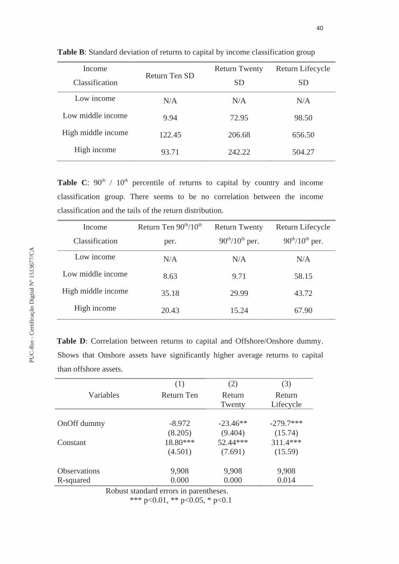
Table B: Standard deviation of returns to capital by income classification group
Income
Classification Return Ten SD
Return Twenty
SD
Return Lifecycle
SD
Low income N/A N/A N/A
Low middle income 9.94 72.95 98.50
High middle income 122.45 206.68 656.50
High income 93.71 242.22 504.27
Table C: 90th / 10th percentile of returns to capital by country and income
classification group. There seems to be no correlation between the income
classification and the tails of the return distribution.
Income
Classification
Return Ten 90th/10th
per.
Return Twenty
90th/10th per.
Return Lifecycle
90th/10th per.
Low income N/A N/A N/A
Low middle income 8.63 9.71 58.15
High middle income 35.18 29.99 43.72
High income 20.43 15.24 67.90
Table D: Correlation between returns to capital and Offshore/Onshore dummy.
Shows that Onshore assets have significantly higher average returns to capital
than offshore assets.
(1) (2) (3) Variables Return Ten Return
Twenty Return
Lifecycle OnOff dummy -8.972 -23.46** -279.7*** (8.205) (9.404) (15.74) Constant 18.80*** 52.44*** 311.4*** (4.501) (7.691) (15.59) Observations 9,908 9,908 9,908 R-squared 0.000 0.000 0.014
Robust standard errors in parentheses. *** p<0.01, ** p<0.05, * p<0.1
PUC
-Rio
-Cer
tific
ação
Dig
italN
º151
3677
/CA

4 Discussion of results 4.1 Discussion of results
When running multivariate regressions of the log of GDP per capita against
the log of returns to capital in section, all specifications in section 3 indicate a
negative correlation, as hypothesized. However, the miniscule economic
significance certainly deserves to be highlighted. The GDP per capita of the
country in which an asset is located is not an important predictor of returns to
capital. By comparison, whether an asset is located onshore or offshore (a purely
geological factor) is far more relevant for the magnitude of the returns under all
specifications and sample periods. The size of the hydrocarbon reserves in also a
far more important determinant of returns to capital in the oil and gas industry
from 1950 to 2016 under all specifications and sample periods. Furthermore,
some institutional factors, namely, level of corruption, level of schooling and
property rights protection possess a statistically significant and positive
correlation with returns to capital, also as hypothesized. Nevertheless, as was the
case with GDP per capita, even though robust statistical correlations were
identified, the correlations were without exception economically quite
insignificant in terms of incremental R-squares.
One may contemplate several potential explanations for the above-
mentioned lack of strong correlations between returns to capital and institutional
quality. To begin with, an important argument is that these rates of return to
capital are, as Caselli and Feyrer (2008) highlighted, so-called “non-reproducible
rates of capital”. For example, the type of rock formations, reservoir quality
(porosity, permeability and the existence of trap) and weather conditions are all
factors that determine the potential revenue (and thus returns to capital) of an oil
and gas asset. Hence, even when holding constant the size of the reservoir and
whether the asset is located onshore or offshore, as is done in this thesis, there are
still a plethora of factors affecting returns to capital that are not country-specific,
but rather geologically determined. As such, this represents an important potential
source of omitted variable bias.
PU
C-R
io-C
ertif
icaç
ãoD
igita
lNº1
5136
77/C
A

Secondly, an important reason that may help explain why returns to capital
are largely independent of country specific variables is that only realized projects
are included in the data. Therefore, capital investments in assets that were not
completed due to high risk or low expected returns are not incorporated in the
data. Since one would expect less developed countries with weaker institutions to
be characterized by higher risk than rich countries, this could be a source for
overestimating the actual returns in poor countries. In other words, a project that
has a marginally positive expected return to capital (and would thus decrease the
average returns in that country) in a poor country would not be completed due to
higher inherent risk. If a geologically similar project were evaluated in a
developed nation, that project could potentially be completed. This is of course
speculative and not observable in the data, but it is consistent with financial
theory, in particular net present value and discount factor theory.
Finally, this thesis finds no evidence that poor countries possess a higher
standard deviation or asymmetry of returns to capital than richer countries in the
oil and gas industry from 1950 to 2016. As stated in the introduction, the standard
deviation and asymmetry of returns were factors that could potentially help
rationalize the difference in returns to capital between poor and rich countries. My
data (counter-intuitively) shows that both the variance and asymmetry are actually
largest in middle-income countries and lowest in lower-middle income countries.
In other words, according to this data, they are not valid or important factors that
may rationalize returns to capital differentials. Supplementary details on
asymmetry can be found in tables 17 and 18 in the appendix.
4.2 Limitations and assumptions
A fundamental assumption is that under conditions approximating perfect
competition in the global capital market, the marginal productivity to capital is
equal to the rate of return to capital. This is an assumption used by Feyrer and
Caselli (2008), which has also been applied in this thesis. It is of course not
entirely realistic, but given the global nature of the oil and gas industry, it might
not be an excessive abstraction, and it is difficult to imagine how the assumption
would create systemically biased results.
PUC
-Rio
-Cer
tific
ação
Dig
italN
º151
3677
/CA

Moreover, the sole manner of controlling for geological differences in this
study is through controlling for the water depth of the oil and gas asset. Albeit
important, this is, however, likely to be an insufficient way of controlling for
geological differences between countries. Other geological characteristics are very
likely to affect the rates of return to capital. This includes, but is not restricted to,
the type of rock formation, porosity, permeability, etc. Future studies could try to
hold these factors constant and verify whether this fundamentally changes the rate
of return differentials between poor and rich countries.
Another limitation of this thesis is the small sample size of countries.
However, this is partly justified by the fact that there simply is not a vast amount
of countries with significant historical production of oil and gas and that countries
with insignificant amounts of production would be more prone to measurement
errors and less precise estimates of variance and asymmetry in returns.
PUC
-Rio
-Cer
tific
ação
Dig
italN
º151
3677
/CA

5 Conclusion
This thesis provides robust evidence demonstrating that poorer countries
enjoyed significantly higher returns to capital than richer countries, in the oil and
gas industry between 1950–2016. Although the results are not particularly
economically significant, this finding is in accordance with what was
hypothesized. Furthermore, the findings providee evidence that certain
institutional factors such as property rights protection, level of corruption and
level of schooling possess a positive and statistically significant correlation with
returns to capital, whilst some other institutional measures tested were not
statistically significant under all specifications. Lastly, neither variance nor
asymmetry in returns look like plausible explanations for returns to capital in the
oil and gas industry, since they are both, differently than hypothesized, lower in
poor countries than rich countries.
The findings in this thesis are important for several reasons. From a
theoretical standpoint, the largely insignificant magnitude of country-specific
variables (as opposed to factors related to the characteristics of the assets)
highlights the importance of adapting economic development theory to account
for sector-specific differences, for example by distinguishing between
reproducible and non-reproducible returns to capital, as emphasized by Feyrer and
Caselli (2008). Lastly, from a practical viewpoint, the results indicate that oil and
gas operators considering making investments in an oil and gas asset should not
be particularly concerned with neither the stage of development nor the
institutional quality of the country in which the asset is located (perhaps, and most
likely, with the exception of very high levels of corruption, big risk of
expropriation or very low levels of schooling). Future studies could further
explore forms of controlling for additional geological factors besides the water
depth of the assets, and, additionally, look for more robust ways of testing which
the validity and magnitude of institutional measures.
PU
C-R
io-C
ertif
icaç
ãoD
igita
lNº1
5136
77/C
A

6
References ACEMOGLU, Daron; DELL, Melissa. Productivity Differences Between and Within Countries. American Economic Journal: Macroeconomics, 2(1), 2010, p.169-88.
AKHTARUZZAMAN, Hajzler & Owen. Does institutional quality resolve the Lucas Paradox? Applied Economics, v.50, Iss. 5, 2018.
ATKINSON, A. B. On the Measurement of Inequality. Journal of Economic Theory, 2, 1970, p.244-63.
BANERJEE, Abhijit V.; MUNSHI, Kaivan. How Efficiently is Capital Allocated? Evidence from the Knitted Garment Industry in Tirupur. Review of Economic Studies, 71(1), 2004, p.19-42.
BANERJEE, Abhijit V.; DUFLO, Esther; MUNSHI, Kaivan. The (Mis)Allocation of Capital. Journal of the European Economic Association, 1(2–3), 2003, p.484-94.
BIGSTEN, Arne; ISAKSSON, Anders; SODERBOM, Mans; COLLIER, Paul et al. Rates of Return on Physical and Human Capital in Africa’s Manufacturing Sector. Economic Development and Cultural Change, 48(4), 2000, p.801-27.
BLACKORBY, C.; DONALDSON, D.; AUERSPERG, M. A New Procedure for the Measurement of Inequality Within and Between Population Subgroups. Canadian Journal of Economics, 14, 1981, p.665-85.
CASELLI, Francesco; FEYRER, James. Marginal Product of capital. IMF, 2006.
CHARLES, Amélie; DARNÉ, Olivier. Volatility Persistence in Crude Oil Markets. Energy Policy, 65 Feb. 2014, p.729-42. Disponível em: http://dx.doi.org/10.1016/j.enpol.2013.10.042.
COULTER, P. Measuring Inequality – A Methodological Handbook. USA: Westview Press, 1989.
COWELL, F. A. Measuring Inequality. Hemel Hempstead: Prentice-Hall/Harvester-Wheatsheaf, 1995.
______. Measurement of Inequality. In: Handbook of Income Distribution. V.1, Eds. A. B. Atkinson and F. Bourguignon. Amsterdam: Elsevier Science, 2000. p.5985.
______; JENKINS, S. P. How Much Inequality Can We Explain? A Methodology and An Application to the USA. Economic Journal, 105, 1995, p.421-30.
David, Henriksen, and Simonovska. 2014. The Risky Capital of Emerging Markets. NBER, Dec. 2014.
DE MEL, Suresh; McKenzie, David; WOODRUFF, Christopher. Returns to Capital in Microenterprises: Evidence from a Field Experiment. The Quarterly Journal of Economics, 123 (4), 2008. 1329-72.
PU
C-R
io-C
ertif
icaç
ãoD
igita
lNº1
5136
77/C
A
HAUGHTON, J.; KHANDKER, S. R. Handbook on Poverty and Inequality. The World Bank, 2009.
HSIEH, Chang-Tai; KLENOW, Peter J. Misallocation and Manufacturing TFP in China and India. Quarterly journal of economics, 2008.
JENKINS, Stephen P. INEQDEC0: Stata Module to Calculate Inequality Indices with Decomposition by Subgroup. Statistical Software Components S366007, Boston College Department of Economics, 1999, revised 22 jan 2015.
KHANDKHER, S. Poverty Manual. Attacking Poverty Program, World Bank Institute, 2002.
LUCAS, Robert. Why Doesn’t Capital Flow from Rich to Poor Countries? American Economic Review, 80(2), 1990, p.92-9.
MANKIW, Gregory; ROMER, David; WEIL, David. A Contribution to the Empirics of Economic Growth. Quarterly Journal of Economics 107(2), 1992, p.407-37.
SHORROCKS, A. F. The Class of Additively Decomposable Inequality Measures. Econometrica, 48(3), 1980, p.613-25.
STEGER, Schularick. Evidence from Two Eras of Financial Globalization. Review of Economics and Statistics, v.92, Issue 4, November 2010, p.756-68.
UDRY, Christopher. Credit Markets in Northern Nigeria: Credit as Insurance in a Rural Economy. World Bank Economic Review, 4(3), 1990, p.251-69.
______; ANAGOL, Santosh. The Return to Capital in Ghana. American Economic Review, 96(2006), 2006, p.388-93.
WHITEHOUSE, E. Measures of Inequality in Stata. Stata Technical Bulletin, 4(23), 1994.
YIN, Libo. Does Oil Price Respond to Macroeconomic Uncertainty? New Evidence. Empirical Economics, 51(3), 2016, p.921.
PUC
-Rio
-Cer
tific
ação
Dig
italN
º151
3677
/CA

7 Appendix
Table 6.1: Correlation between log of returns to capital and GDP per capita.
Shows a non-robust relationship.
(1) (2) (3) Variables Log Return
Ten Log Return
Twenty Log Return Lifecycle
GDP per capita (IHME) 3.95e-06*** 7.68e-07 -8.05e-06*** (1.22e-06) (1.28e-06) (2.12e-06) Constant 1.823*** 2.580*** 3.273*** (0.0231) (0.0239) (0.0318) Observations 4,081 4,023 3,968 R-squared 0.003 0.000 0.006
Robust standard errors in parentheses. *** p<0.01, ** p<0.05, * p<0.1
Table 6.2: Correlation between log of returns to capital and log of GDP per capita.
For return twenty and return lifecycle one may see that assets located in countries
with lower GDP do indeed exhibit (slightly) higher returns to capital.
(1) (2) (3) Variables Log Return
Ten Log Return
Twenty Log Return Lifecycle
Log of GDP per capita (IHME)
-0.00799 -0.0446*** -0.163***
(0.00994) (0.0108) (0.0128) Constant 1.930*** 2.943*** 4.475*** (0.0820) (0.0870) (0.103) Observations 4,081 4,023 3,968 R-squared 0.000 0.004 0.033
Robust standard errors in parentheses. *** p<0.01, ** p<0.05, * p<0.1
PU
C-R
io-C
ertif
icaç
ãoD
igita
lNº1
5136
77/C
A

Table 7: Summary of correlations between returns to capital measures and various
measures of institutional quality (Significant and robust results are reported in
more detail in separate tables)
Variable Log Return
Ten
Log Return
Twenty
Log Return
Lifecycle
Bureaucratic delays 0.0115 -0.0228*** -0.0140
Infrastructure quality 0.00760 -0.00932* 0.00919
Corruption level (see table 7) 0.0228*** 0.0342*** 0.0877***
Tax Evasion 0.0819*** -0.0133 -0.133***
Level of Schooling (see table 8) 0.101*** 0.0852*** 0.302***
Adult illiteracy rate (see
table 9) 0.0146*** 0.00911*** 0.00690***
Av.Gov.wages/GDP per cap
(see table 10) 0.113*** 0.0880*** 0.103***
Political rights index -0.0235*** -0.0137** 0.00767
Democracy Score 0.0108*** 0.00519*
0.0152*** Property Rights Index (see
table 11) 0.0240** 0.0185* 0.0509***
Business Regulation Score
(see table 12) 0.0552*** 0.0532*** 0.108***
*** p<0.01, ** p<0.05, * p<0.1
PUC
-Rio
-Cer
tific
ação
Dig
italN
º151
3677
/CA

Table 8: Correlation between returns to capital and Level of corruption (1) (2) (3) Variables Log Return
Ten Log Return
Twenty Log Return Lifecycle
Corruption level 0.0228*** 0.0342*** 0.0877*** (0.00524) (0.00579) (0.00878) Constant 1.688*** 2.384*** 2.780*** (0.0404) (0.0432) (0.0606) Observations 8,136 8,079 7,963 R-squared 0.002 0.004 0.013
Robust standard errors in parentheses *** p<0.01, ** p<0.05, * p<0.1
Table 9: Correlation between returns to capital and Level of schooling (1) (2) (3) Variables Log Return
Ten Log Return
Twenty Log Return Lifecycle
Level of schooling 0.101*** 0.0852*** 0.302*** (0.0260) (0.0277) (0.0376) Constant 1.597*** 2.416*** 2.761*** (0.0537) (0.0568) (0.0733) Observations 6,955 6,897 6,792 R-squared 0.002 0.001 0.007
Robust standard errors in parentheses *** p<0.01, ** p<0.05, * p<0.1
Table 10: Correlation between returns to capital and Adult illiteracy rate (1) (2) (3) Variables Log Return
Ten Log Return
Twenty Log Return Lifecycle
Adult illiteracy rate 0.0146*** 0.00911*** 0.00690*** (0.00127) (0.00140) (0.00179) Constant 1.454*** 2.380*** 3.104*** (0.0396) (0.0438) (0.0534) Observations 3,669 3,612 3,576 R-squared 0.033 0.012 0.004
Robust standard errors in parentheses *** p<0.01, ** p<0.05, * p<0.1
PUC
-Rio
-Cer
tific
ação
Dig
italN
º151
3677
/CA
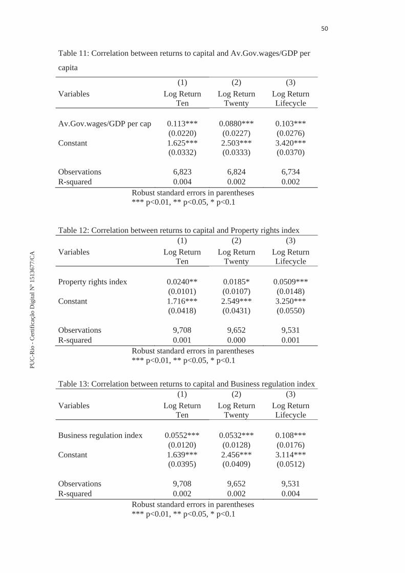
Table 11: Correlation between returns to capital and Av.Gov.wages/GDP per
capita
(1) (2) (3) Variables Log Return
Ten Log Return
Twenty Log Return Lifecycle
Av.Gov.wages/GDP per cap 0.113*** 0.0880*** 0.103*** (0.0220) (0.0227) (0.0276) Constant 1.625*** 2.503*** 3.420*** (0.0332) (0.0333) (0.0370) Observations 6,823 6,824 6,734 R-squared 0.004 0.002 0.002
Robust standard errors in parentheses *** p<0.01, ** p<0.05, * p<0.1
Table 12: Correlation between returns to capital and Property rights index (1) (2) (3) Variables Log Return
Ten Log Return
Twenty Log Return Lifecycle
Property rights index 0.0240** 0.0185* 0.0509*** (0.0101) (0.0107) (0.0148) Constant 1.716*** 2.549*** 3.250*** (0.0418) (0.0431) (0.0550) Observations 9,708 9,652 9,531 R-squared 0.001 0.000 0.001
Robust standard errors in parentheses *** p<0.01, ** p<0.05, * p<0.1
Table 13: Correlation between returns to capital and Business regulation index (1) (2) (3) Variables Log Return
Ten Log Return
Twenty Log Return Lifecycle
Business regulation index 0.0552*** 0.0532*** 0.108*** (0.0120) (0.0128) (0.0176) Constant 1.639*** 2.456*** 3.114*** (0.0395) (0.0409) (0.0512) Observations 9,708 9,652 9,531 R-squared 0.002 0.002 0.004
Robust standard errors in parentheses *** p<0.01, ** p<0.05, * p<0.1
PUC
-Rio
-Cer
tific
ação
Dig
italN
º151
3677
/CA

Table 14: Summary of correlations between returns to capital measures and the
world bank’s dataset of institutional quality between years 1996-2016.
Institutional Variable Log Return
Ten
Log Return Twenty Log Return
Lifecycle
Control of corruption 0.0521*** 0.0281*** 0.0115
Government
Effectiveness 0.0538*** -0.00501 -0.0563***
Corruption level 0.103*** 0.0770*** 0.0142
Political Stability 0.0567*** 0.0196 -0.00157
Robust standard errors in parentheses *** p<0.01, ** p<0.05, * p<0.1
Table 15: Shows the three different average returns to capital of all assets in each
country and income group in detail.
COUNTRY Return Ten
Average
Return Twenty
Average
Return Lifecycle
Average
United Arab Emirates 15.87 51.28 507.19
Angola 8.87 14.51 23.09
Argentina 15.31 46.62 66.82
Australia 9.23 27.08 23.97
Azerbaijan 5.95 13.61 69.04
Brazil 11.78 35.80 494.87
Chile 6.58 14.84 32.06
China 12.45 25.52 66.10
Congo 7.30 17.15 21.10
Denmark 13.72 73.79 45.70
Algeria 115.87 193.80 327.85
Egypt 0.55 1.20 114.49
Great Britain 11.14 70.74 23.65
PUC
-Rio
-Cer
tific
ação
Dig
italN
º151
3677
/CA
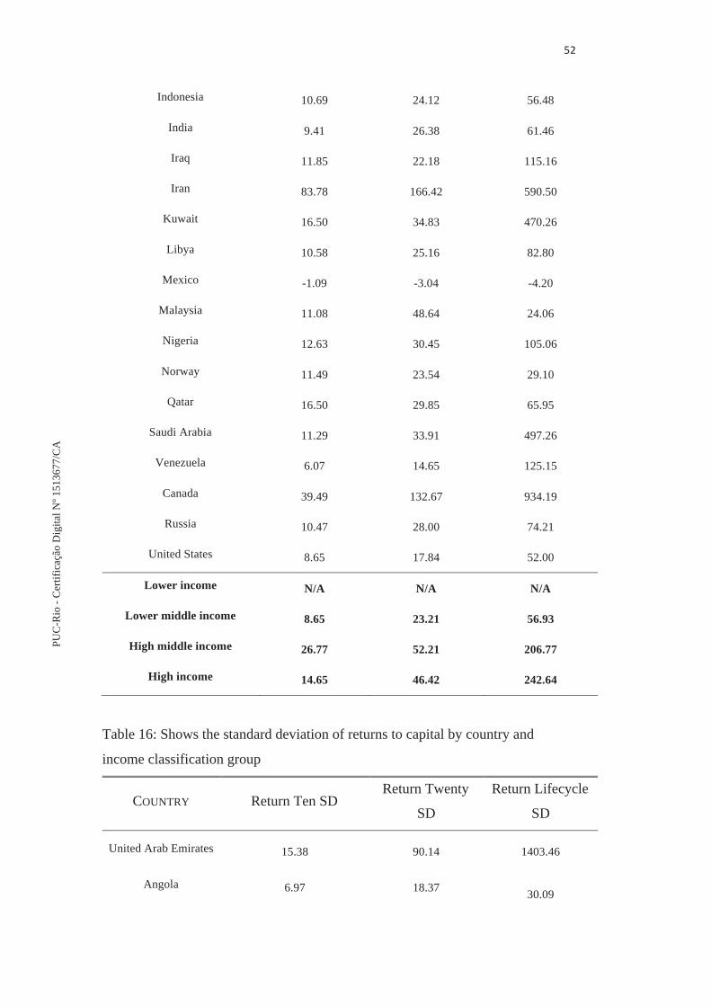
Indonesia 10.69 24.12 56.48
India 9.41 26.38 61.46
Iraq 11.85 22.18 115.16
Iran 83.78 166.42 590.50
Kuwait 16.50 34.83 470.26
Libya 10.58 25.16 82.80
Mexico -1.09 -3.04 -4.20
Malaysia 11.08 48.64 24.06
Nigeria 12.63 30.45 105.06
Norway 11.49 23.54 29.10
Qatar 16.50 29.85 65.95
Saudi Arabia 11.29 33.91 497.26
Venezuela 6.07 14.65 125.15
Canada 39.49 132.67 934.19
Russia 10.47 28.00 74.21
United States 8.65 17.84 52.00
Lower income N/A N/A N/A
Lower middle income 8.65 23.21 56.93
High middle income 26.77 52.21 206.77
High income 14.65 46.42 242.64
Table 16: Shows the standard deviation of returns to capital by country and
income classification group
COUNTRY Return Ten SD Return Twenty
SD
Return Lifecycle
SD
United Arab Emirates
15.38
90.14 1403.46
Angola 6.97 18.37
30.09
PUC
-Rio
-Cer
tific
ação
Dig
italN
º151
3677
/CA

Argentina 68.22 150.62
140.66
Australia 8.71 87.61
52.31
Azerbaijan 6.93 14.84
65.50
Brazil 19.72 78.44
2344.13
Chile 4.28 28.69
69.82
China 11.61 24.16
153.83
Congo 25.81 69.30
33.75
Denmark 16.01 201.52
40.08
Algeria 964.68 1524.31
1792.87
Egypt 0.68 1.48
160.61
Great Britain 9.18 862.42
37.89
Indonesia 9.68 60.55
149.19
India 7.70 36.79
103.97
Iraq 14.97 26.32
180.30
Iran 149.78 276.45
1067.73
Kuwait 21.68 33.76
382.60
Libya 9.09 21.03
101.82
Mexico 3.00 7.76
14.85
Malaysia 9.28 286.03
21.58
Nigeria 9.49 38.09
145.38
Norway 14.15 32.13
37.56
Qatar 16.00 22.61
50.41
Saudi Arabia 13.72 37.75
721.64
Venezuela 9.09 16.58
137.91
Canada 924.58 1300.15
2307.56
Russia 35.61 76.86
119.12
United States 12.65 59.44
366.06
PUC
-Rio
-Cer
tific
ação
Dig
italN
º151
3677
/CA
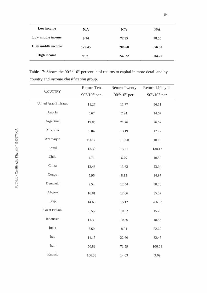
Low income N/A N/A N/A
Low middle income 9.94 72.95 98.50
High middle income 122.45 206.68 656.50
High income 93.71 242.22 504.27
Table 17: Shows the 90th / 10th percentile of returns to capital in more detail and by
country and income classification group.
COUNTRY Return Ten
90th/10th per.
Return Twenty
90th/10th per.
Return Lifecycle
90th/10th per.
United Arab Emirates 11.27 11.77 56.11
Angola 5.67 7.24 14.67
Argentina 19.85 21.76 76.62
Australia 9.04 13.19 12.77
Azerbaijan 196.39 115.00 18.18
Brazil 12.30 13.71 138.17
Chile 4.71 6.79 10.50
China 13.48 13.62 23.14
Congo 5.96 8.13 14.97
Denmark 9.54 12.54 38.86
Algeria 16.81 12.66 35.07
Egypt 14.65 15.12 266.03
Great Britain 8.55 10.32 15.20
Indonesia 11.39 10.56 18.56
India 7.60 8.04 22.62
Iraq 14.15 22.60 32.45
Iran 50.83 71.59 106.68
Kuwait 106.33 14.63 9.69
PUC
-Rio
-Cer
tific
ação
Dig
italN
º151
3677
/CA
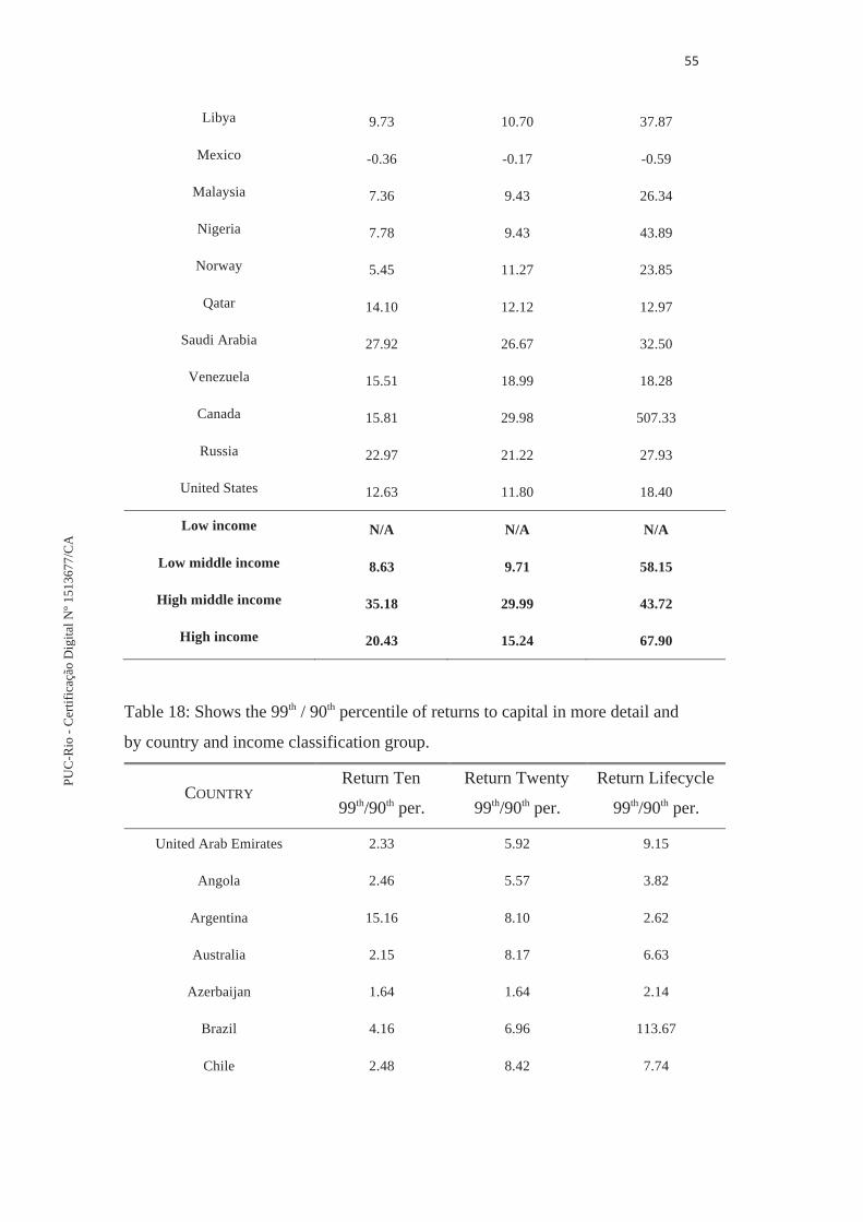
Libya 9.73 10.70 37.87
Mexico -0.36 -0.17 -0.59
Malaysia 7.36 9.43 26.34
Nigeria 7.78 9.43 43.89
Norway 5.45 11.27 23.85
Qatar 14.10 12.12 12.97
Saudi Arabia 27.92 26.67 32.50
Venezuela 15.51 18.99 18.28
Canada 15.81 29.98 507.33
Russia 22.97 21.22 27.93
United States 12.63 11.80 18.40
Low income N/A N/A N/A
Low middle income 8.63 9.71 58.15
High middle income 35.18 29.99 43.72
High income 20.43 15.24 67.90
Table 18: Shows the 99th / 90th percentile of returns to capital in more detail and
by country and income classification group.
COUNTRY Return Ten
99th/90th per.
Return Twenty
99th/90th per.
Return Lifecycle
99th/90th per.
United Arab Emirates 2.33 5.92 9.15
Angola 2.46 5.57 3.82
Argentina 15.16 8.10 2.62
Australia 2.15 8.17 6.63
Azerbaijan 1.64 1.64 2.14
Brazil 4.16 6.96 113.67
Chile 2.48 8.42 7.74
PUC
-Rio
-Cer
tific
ação
Dig
italN
º151
3677
/CA

China 2.27 1.85 5.00
Congo 4.46 8.49 3.74
Denmark 2.01 8.86 1.49
Algeria 38.51 26.24 5.43
Egypt 1.00 1.00 1.00
Great Britain 1.91 3.64 6.03
Indonesia 1.83 3.23 4.74
India 1.97 3.21 4.20
Iraq 4.31 2.17 2.54
Iran 3.77 2.87 3.58
Kuwait 1.21 1.17 1.25
Libya 2.28 1.67 1.86
Mexico 1.67 2.50 5.37
Malaysia 2.08 11.71 2.25
Nigeria 1.71 2.47 2.98
Norway 5.68 4.53 4.06
Qatar 1.71 1.62 1.14
Saudi Arabia 1.88 1.25 4.16
Venezuela 4.15 2.40 2.31
Canada 2.86 7.48 2.55
Russia 2.79 4.00 3.14
United States 3.10 3.72 9.66
Low income N/A N/A N/A
Low middle income 2.22 5.10 3.25
High middle income 6.55 5.23 14.50
High income 3.54 5.24 4.71
PUC
-Rio
-Cer
tific
ação
Dig
italN
º151
3677
/CA

Table 19: Descriptive statistics for the measures of GDP per capita from IMHE
(Given in USD and normalized to 2005 and PPP) from 1950 to 2016.
COUNTRY Average SD Minimum Maximum
United Arab Emirates 56193 14625.23 34652 80779
Angola 3811 1383.719 1988 6123
Argentina 8852 1883.721 5469 16179
Australia 29601 7452.065 10679 41723
Azerbaijan 3740 2590.375 846 11421
Brazil 7125 2346.822 2259 11808
Chile 8555 4151.68 3413 15662
China 4341 3103.167 206 10467
Congo 3134 618.2883 1225 3714
Denmark 23192 8576.685 9547 36738
Algeria 5100 1263.975 2744 7624
Egypt 2829 1528.004 1112 6471
Great Britain 27679 6431.241 10107 35613
Indonesia 2354 1176.747 575 5178
India 1878 1119.193 541 4354
Iraq 4588 1423.372 2028 9296
Iran 7403 2352.306 2744 11137
Kuwait 60672 29021.88 23930 115403
Libya 18134 7335.086 3665 32449
Mexico 9115 2846.069 3900 14756
Malaysia 747 381.4898 154 1269
Nigeria 1590 410.2086 986 2551
Norway 36264 14030.08 10033 51644
Qatar 85291 23045.21 45958 124998
PUC
-Rio
-Cer
tific
ação
Dig
italN
º151
3677
/CA

Saudi Arabia 18202 7081.96 5453 31696
Venezuela 8972 1170.762 6747 12106
Canada 24005 8531.667 11180 38229
Russia 10247 3070.476 4964 16944
United States 28218 7612.025 13168 48242
PUC
-Rio
-Cer
tific
ação
Dig
italN
º151
3677
/CA


