
1
OPTIMAL ALGORITHM FOR THE DEMAND ROUTING PROBLEM IN
MULTICOMMODITY FLOW DISTRIBUTION NETWORKS WITH
DIVERSIFICATION CONSTRAINTS AND CONCAVE COSTS
Abstract.-
Distribution problems are of high relevance within the supply chain system. In real life
situations various different commodities may flow in the distribution process.
Furthermore, the connection between production and demand centres makes use of
complex mesh networks that can include diversification constraints to avoid
overcharged paths. In addition, the consideration in certain situations of economies of
scale gives rise to non-linear cost functions that make it difficult to deal with an optimal
routing scheme. This problem is well represented by the multicommodity flow
distribution networks with diversification constraints and concave costs (MFDCC)
problem. Here we present an optimal algorithm based on the Kuhn-Tucker optimality
conditions of the problem and capable of supplying optimal distribution routes in such
complex networks. The algorithm follows an iterative procedure. Each iteration
constructive solutions are checked with respect to the Kuhn-Tucker optimality
conditions. Solutions consider a set of paths transporting all the demand allowed by its
diversification constraint (saturated paths), a set of empty paths, and an indicator path
transporting the remaining demand to satisfy the demand equation. The algorithm
reduces the total cost in the network in a monotonic sequence to the optimum. The
algorithm was tested in a trial library and the optimum was reached for all the instances.
The algorithm showed a major dependency with respect to the number of nodes and
arcs of the graph, as well as the density of arcs in the graph.
Keywords: demand routing; concave cost; distribution network; Kuhn Tucker
conditions
1. Introduction
Distribution problems are of high relevance within the supply chain system. One of the
principal root problems in the family is the transportation problem that was introduced
in 1941 by Hitchcock (Hitchcock, 1941). This has been researched extensively due to its
importance and the wide range of applications it has. The transportation problem
involves a network with a group of production centres willing to send their commodity
to a group of demand centres through a set of arcs with linear costs.
However, in real life situations various different commodities may flow instead of just
one commodity (e.g. Kengpol et al., 2011). Furthermore, each production centre is not
connected with each demand centre using a single arc but rather with a mesh network of
different arcs (Ubeda et al., 2010). Certain cases cannot be correctly modelled using a
linear cost function and require a more complex way of modelling (Tsao et al. 2010).
Sometimes more accurate results can be achieved with concave cost functions. This
situation arises when dealing with economies of scale which are very common in many
fields such as freight distribution and demand routing systems, and even other
technological fields such as telecommunication networks.
2
In this paper, we consider a mesh network with a set of nodes as the origin of demand
and a set of nodes as the demand destination. Each pair of nodes constitutes an origin-
destination pair which is known as a specific commodity, converting the problem into a
multicommodity flow problem. Additionally, the costs in arcs are modelled by concave
costs. Lastly, we propose the diversification constraints needed to prevent the arcs from
becoming extremely loaded which can produce malfunction effects on the network and
may arise when concave costs are involved as a result of the benefits offered by
economies of scale. This type of constraint increases the survivability and reliability of
the networks.
Distribution problems with concave costs are NP-Hard and their optimal solution cannot
be found in polynomial time. Several authors have proposed approximate methods to
tackle this problem, such as the linear approximation by Thach (1992), the lagrangian
relaxation by Larsson et al. (1994), or the dynamic programming approach by Zangwill
(1968), Florian and Klein (1971) and Burkard et al. (2001). Metaheuristic approaches
have also been tested although mainly in telecommunication network problems
(Kapsalis et al, 1993; Dengiz et al, 1997; Altiparmak et al, 2003; Zhou and Gen, 2003).
In a more general case, Yan and Luo (1999) developed a heuristic based on simulated
annealing and threshold acceptance, and Altiparmark and Karaoglan (2008) proposed a
tabu approach to solve the transportation problem with concave costs. Here, we have
developed an optimal approach based on the optimality Kuhn-Tucker conditions of the
mathematical formulation of the problem.
The paper then defines the problem and its mathematical formulation in Section 2.
Section 3 presents the Kuhn-Tucker optimality conditions for the demand routing
problem in multicommodity flow networks with diversification constraints and concave
costs that has been described in the previous section. Next, the solution based on the
optimality constraints demand routing algorithm is proposed is Section 4. The results
for a trial library with 27 generated instances are presented in Section 5 and the detailed
procedure for an example network is developed. Finally, the main conclusions are
presented in Section 6.
2. Problem definition and formulation
Given a graph G=(N,E) where N is the set of nodes and E the set of arcs, a set of
commodities K is considered and represents every origin-destination pair of demand.
We define each arc of the network as e∈E and the set of paths connecting every origin-
destination pair is given by P(k). A subset of this set is given by the arc-disjoint paths,
Pd(k).
Let γk be the demand volume for each origin-destination pair, k, and δk the
diversification parameter for each pair k, so that the demand of pair k is routed along
1 kδ different paths. As paths and arcs are pre-computed, ϕeh is a binary parameter
that determines if arc e is on path h.
The variables of the problem are the demand fraction related to the origin-destination
pair k that is routed on path h, which is a continuous variable given by pkh, and the total
3
flow transported on arc e, including the total amount of flow from all the commodities
on the arc, which is a continuous variable given by xe.
Owing to the nature of the problem described, numerous concave cost functions can be
considered. We used the objective function given by ( )e e e ec x d x= for arc e, where xe
has been previously explained and de means the per unit variable cost corresponding to
the arc. We selected this function because it provides a widely acknowledged basis of
analysis of scale economies’ effect in transportation problems, and because it is taken as
a representative cost function very similar to many transportation cost functions in
practice (see detailed arguments in LeBlanc 1976; Larsson et al. 1994; Yan and Luo
1999; and Altiparmak and Karaoglan 2008). The cost concave function is, therefore, a
differentiable function. Note that the objective function is used to provide comparable
numerical examples in the subsequent results section. The selection of this function
does not condition the methodology and developed algorithm, because the objective
function only affects the procedure for the calculation of the derivative providing
numerical data.
As a result, the demand routing problem in multicommodity flow networks with
diversification constraints and concave costs (MFDCC problem) can be formulated as:
( )
( )
( )
Minimize
, 1
, 2
,
e e
e E
e eh kh
k K h ( k )
kh k
h ( k )
kh k k
c x
s.t. :
x p e E
p k K
p h
∈
∈ ∈Ρ
∈Ρ
= ϕ ∀ ∈
= γ ∀ ∈
≤ δ γ ∀ ∈ Ρ
∑
∑ ∑
∑
( ) ( ) , 3
0 , 0
d
e kh
k k K
x p
∀ ∈
≥ ≥
Constraint (1) calculates the total amount of flow on the arc e; constraint (2) ensures
that the demand for every origin-destination pair is met; and constraint (3) ensures that
the demand is routed along 1 kδ alternative paths. Set Pd(k) represents all the feasible
disjoint paths for each origin-destination pair. The “disjoint” concept is important and
can be weakly imposed on the arcs or strongly imposed on the nodes. Here, we have
chosen the arc diversification concept because in most cases it is normally only
necessary to take this weak constraint into consideration. Using an example from
telecommunications, disjoint arcs can be used to model reality, since the optical cross-
connect (OXC) in an all-optical WDM mesh network is seldom broke. The OXC is a
device which switches an optical signal from an incoming fibre to an outgoing fibre on
the same wavelength. So, constraint (3) is equivalent to:
� ( ) ( ) , d
kh kp i, j h , h P k : k K≤ δ ∀ ∈ ∈ ∈ , constraint for arc-disjoint paths
� ( ) , d
kh kp j h , h P k : k K≤ δ ∀ ∈ ∈ ∈ , constraint for node-disjoint paths
depending on what is being considered and as explained above, we are looking at
4
constraints for arc-disjoint paths.
3. Kuhn Tucker conditions for the demand routing problem in multicommodity
flow networks with diversification constraints and concave costs
Every solution verifying the necessary and sufficient Kuhn-Tucker conditions of any
problem will be the optimal solution of problem. This fact is proven for linear or non-
linear problems since they are global optimality conditions. Additionally, duality theory
can be regarded as a particular case of the Kuhn-Tucker conditions for linear problems.
See classic theory such as Hillier and Lieberman (1977), Nocedal and Wright (1999),
Avriel (2003) for detailed explanations on Kuhn-Tucker conditions. Appendix 1 depicts
a general overview on the Kuhn-Tucker necessary optimality conditions and their
detailed corresponding application to MFDCC problem, and appendix 2 depicts the
equivalent general overview and detailed application of the Kuhn-Tucker sufficient
optimality conditions to the MFDCC problem.
Next, we re-formulate MFDCC problem to specify the objective function in terms of pkh
variables. This can be done because pkh and xe are inter-related by constraint (2).
Therefore, constraint (2) is included in the objective function to re-formulate the
problem and subsequently formulate the Kuhn-Tucker necessary optimality conditions:
( ) ( ) ( )
( )
= 0 , (free multipliers)
0 , , (non-negative multip
∈
∈
≡ ≡
γ − ∀ ∈ ← µ
− δ γ ≤ ∀ ∈ ∀ ∈ ←
∑
∑
kh
h P(k)
e e
e E
k k
d
kh k k kh
p
Minimize c x Minimize C x Minimize C p
s.t. :
k K
p · h P k k K v
( )
liers)
0 , , (non-negative multipliers)− ≤ ∀ ∈ ∀ ∈ ←d
kh khp h P k k K u
Kuhn-Tucker conditions state that all ( )dh P k∈ and k K∈ can be written as:
kh khk
kh
k khkkh
khkh
C(p) = u v
p
( · ) · = 0p v
· = 0p u
-
-
∂µ
∂
γδ
-
(4)
By calculating the cost function variation related to the demand fraction routed along
path h, we replace the expression of the total cost in the network C(p) with the sum of
the costs of the flows in the arcs, and then we substitute the value of the flow xe
accordingly with equation (1):
5
ϕϕ eheeEe
ehkhP(k)hKk
kh
eeEe
kh
e
e
ee
Eekh
ee
Eekh
eeEe
kh
)x(c = pp
)x(c =
= p
x
x
)x(c =
p
)x(c =
p
)x(c =
p
C(p)
'·' ∑
∑∑
∂
∂∑
∂
∂
∂
∂∑
∂
∂∑
∂
∑∂
∂
∂
∈∈∈∈
∈∈
∈
(5)
that corresponds to the sum of cost variations on the arcs belonging to path h. The
optimality conditions are thus enforced on the increase of the cost and not on its
absolute value. By analysing these conditions, we can differentiate the meaning of the
conditions and three different types of paths are found:
� Case 1: the origin-destination pair does not use path h to establish a
communication.
kh khkh
khk
kh
e khe eh k
e E
ee eh k
e E
= 0 0 and = 0 p u v
C(p) - = 0u
p
c' ( ) - = 0x u
c' ( ) x
∈
∈
⇒ ≥
∂≥µ
∂
≥ϕ µ
≥ϕ µ
∑
∑
(6)
Therefore, the sum of the cost variations corresponding to the arcs on the empty
or void paths that are not used by the origin-destination pair k is greater than kµ .
� Case 2: the origin-destination pair uses path h to establish a communication.
Here, two possibilities arise:
o Case 2.a: the arc transports all the flow allowed by the diversification
constraint. There are 1
1k
− δ
paths in this case. In this case, the Kuhn-
Tucker conditions are reduced to:
k kh khkh
khk
kh
e khe eh k
e E
ee eh k
e E
= = 0 and 0 p u v
C(p) - = - 0v
p
c' ( ) - = - 0x v
c' ( ) x
∈
∈
⇒ ≥δ
∂≤µ
∂
≤ϕ µ
≤ϕ µ
∑
∑
(7)
The sum of the cost variations corresponding to the arcs on the saturated
paths used by the origin-destination pair k, i.e. ( )dh P k∈ , is upper
bounded by kµ .
6
o Case 2.b: the arc transports less flow than the limitation imposed by the
diversification constraint. There is only one path that verifies this
situation, which is:
k kh khkh
k
kh
e eh k
e E
< = 0 and = 0p u v
C(p) - = 0
p
c'( ) = x∈
⇒δ
∂µ
∂
ϕ µ∑
(8)
The sum of the cost variations corresponding to the arcs on the path that
transports a positive amount of flow but below the maximum value
imposed by the diversification constraint related to the origin-destination
pair k is equal to kµ . This path will be known as the indicator path. This
is a concept that appears in similar terms in the traditional transportation
problem (when links in the graph are grouped into three sets; a set of
slacks equal to zero; a set of slacks equal to the capacity, that is empty
arcs; and one link with an amount of flow equal to the difference
between the demand and the sum of all the flow in arcs with slack equal
to zero). We originally introduced this term in Cortes et al. (2006).
The existence of only one indicator path is also intuitive. Note that if there was a
cheaper path, that path would be full, and if there was a more expensive path it should
be empty, and so the path in the middle separating cheap paths from expensive paths
should transport the rest of demand to satisfy the demand equation. There could be only
two particular cases: (i) the rest of demand is equal to the capacity, so it would be full,
(ii) there is a draw between two paths, corresponding to a case of alternative solutions,
but the solution cost would be the same, and these two cases do not condition the
algorithm procedure that will be later detailed in section 4, because either of the
drawing paths could act as indicator as a matter of fact.
In summary:
� For every origin-destination pair, k, cheap, expensive and indicator paths can be
considered.
The cheap paths are saturated and transport as much flow as possible, i.e.:
kh k kp ·= δ γ .
The expensive paths are empty and do not transport flow, i.e.: 0kh
p =
The indicator path transports the necessary amount of flow to satisfy the demand
equation (eq. 2), which is less than k k·δ γ and more than 0.
� The transported product that flows through the communication paths in order to
satisfy the demand of all origin-destination pairs will be optimum if the
“separator cost concept” is given by ek eh
e E
c'( ) x∈
=µ ϕ∑ in the indicator path.
In this way, the Kuhn-Tucker multipliers include the following meanings:

7
'hk ic ∼µ It is a concept associated with the value of the derivative of the cost
function along the indicator path.
( )hshkh c -c vi
''∼ It is a concept associated with the deviation between the values of the
derivative of the cost function of the indicator path and each
saturated path. The Kuhn-Tucker optimality conditions determine
that this deviation must be positive for every ( )dh P k∈ and k K∈ .
( )iv hhkh c -c u ''∼ It is a concept associated with the deviation between the values of the
derivative of the cost function of each empty path and the indicator
path. The Kuhn-Tucker optimality conditions determine that this
deviation must be positive for every ( )dh P k∈ and k K∈ .
4. Demand routing algorithm
After having explained the Kuhn-Tucker optimality conditions above, this section
describes an optimal iterative algorithm that can be used to solve the demand routing
problem in multicommodity flow networks with diversification constraints and concave
costs. The algorithm converges to the optimal process by reducing the non-feasibility
after every iteration.
The algorithm needs to pre-compute all the paths of the graph between a pair of nodes.
This is done with an algorithm based on a depth first search routine that is shown in
appendix 4. Although the problem of finding all the paths between every pair of nodes
in a graph is a NP-Hard problem, we consider sparse networks, so that results can be
obtained quickly as the result section shows next.
Step 1. Initialisation. Greedy heuristic
The procedure is based on the k shortest disjoint path algorithm provided by Kleinberg
(1996).
1. Order the origin-destination pairs according to the demand volume, γk.
Subsequently, following that order:
2. For each origin-destination pair, k:
a. For a number of times equal to 1 kδ -1
i. Calculate the shortest path between the origin o(k) and the
destination d(k).This is a saturated path hs∈ Pd(k).
ii. Assign a volume of demand equal to δ k·γk.
iii. Erase the path to search for a new disjoint path.
b. Calculate the shortest path between the origin o(k) and the destination
d(k), and assign the remaining demand to satisfy equation (2). This is the
candidate indicator path hi∈ Pd(k).
In the greedy heuristic the costs of the arcs are simplified to ( )e e ec x d= in order to
calculate the shortest paths. Dijkstra’s algorithm can, therefore, be applied. This initial
flow load provides a determined level of flow along the paths, pkh0, corresponding to a
8
specific level of flow load on the arcs of the network, xe0.
We used this greedy heuristic with the objective of providing an initial set of disjoint
paths. It starts selecting a set of edge-disjoint paths that provides an initial set that is
only considered as the seed of the algorithm. After that, the iterative algorithm (next
steps of the iterative routine that forces to accomplish the Kuhn-Tucker conditions)
guides the flow in the paths from that seed to optimality by testing the optimality
conditions for all the paths of the graph connecting such pair k. The main reason to use
this shortest path based initialization algorithm is to generate a seed quickly.
Furthermore, as the shortest path tries to minimise the cost between a pair of nodes, this
can be taken as a reasonably good initial solution following the arguments detailed in
Kleinberg (1996).
Step 2.Checking the Kuhn-Tucker optimality conditions
The Kuhn-Tucker conditions are checked for every origin-destination pair, k. The
condition is given by (9):
( ) ( ) ( )( ) ( ) ( ){ } ( )
( ) ( )
0 0 0
0
for every saturated path indicator path empty or void path
where
s i vh kh h kh h kh
d
s i v
h kh e e eh
e E
c' p c' p c' p
h h ,h ,h P k
c' p c' x∈
≤ ≤
= ∈
= ⋅ϕ∑ (9)
After the saturated and indicator paths have been obtained (as a result of step 1 or the
iterative process), we have to check the conditions for all the empty paths of the graph
(it has to be taken into account that the condition must be verified for all the empty
paths in the graph as well. These do not necessarily have to be disjoint paths).
The iterative process comes to an end if the optimality conditions are checked;
otherwise, the procedure follows step 3.
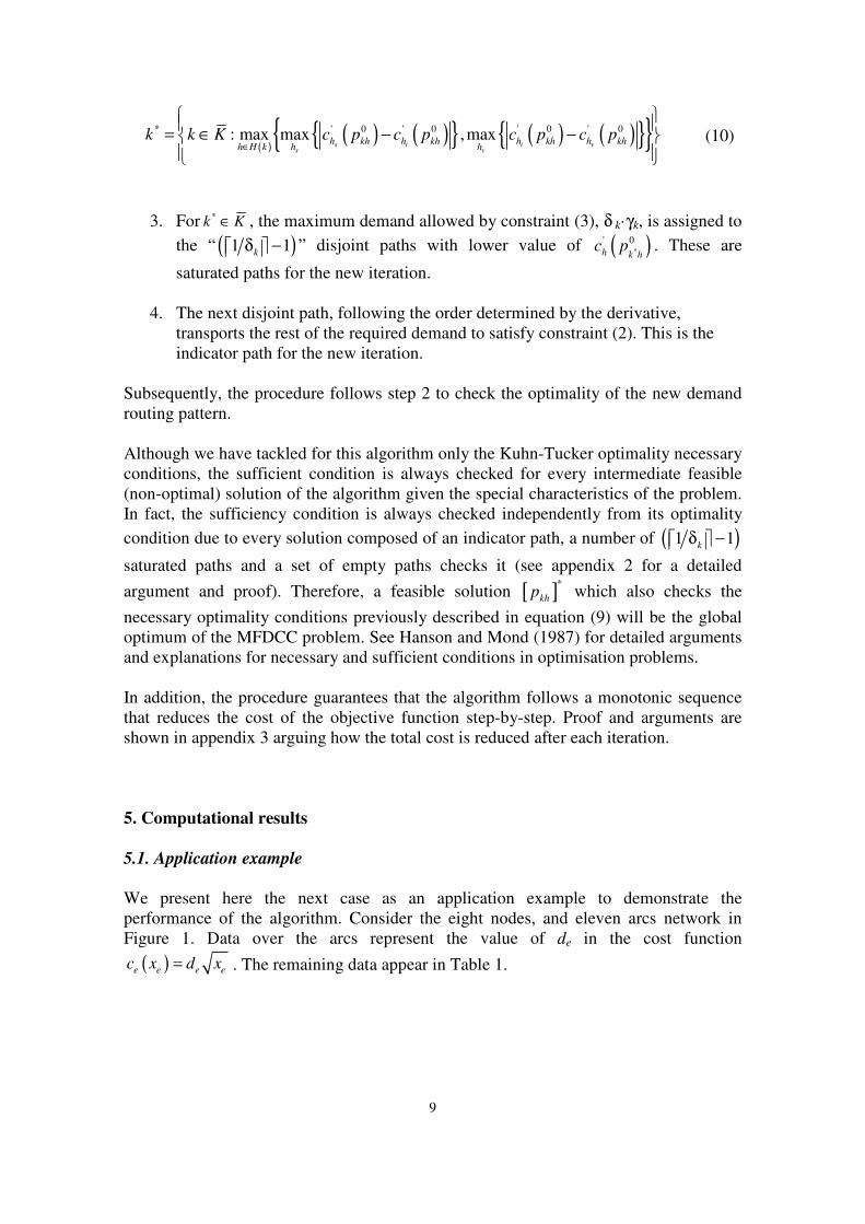
Step 3. Iteration
All the origin-destination pairs that do not check the optimality conditions shape the set
K (we say that k K∈ if pair k does not verify the Kuhn-Tucker conditions, i.e. eq. 9).
For these pairs, the set H(k) is defined as the paths that do not check the condition of
such pair, k K∈ . Next procedure is followed:
1. For every k K∈ , paths in H(k) are arranged in increasing order according to the
derivative of the cost function assessed for the previous (step 2) demand routing
pattern, 0
khp . That is, ( ) ( )0 0' 'h kh e e eh
e E
c p c x∈
= ⋅ϕ∑ is calculated for every h∈ H(k),
for every k K∈ .
2. Origin-destination pair k* is selected as it is the pair that provides the highest
absolute deviation with respect to the optimality conditions, as calculated in
(10).
9
( )( ) ( ){ } ( ) ( ){ }{ }* ' 0 ' 0 ' 0 ' 0: max max ,max
s i i vs v
h kh h kh h kh h khh H k h h
k k K c p c p c p c p∈
= ∈ − −
(10)
3. For *k K∈ , the maximum demand allowed by constraint (3), δ k·γk, is assigned to
the “ ( )1 1k
δ − ” disjoint paths with lower value of ( )*
' 0
h k hc p . These are
saturated paths for the new iteration.
4. The next disjoint path, following the order determined by the derivative,
transports the rest of the required demand to satisfy constraint (2). This is the
indicator path for the new iteration.
Subsequently, the procedure follows step 2 to check the optimality of the new demand
routing pattern.
Although we have tackled for this algorithm only the Kuhn-Tucker optimality necessary
conditions, the sufficient condition is always checked for every intermediate feasible
(non-optimal) solution of the algorithm given the special characteristics of the problem.
In fact, the sufficiency condition is always checked independently from its optimality
condition due to every solution composed of an indicator path, a number of ( )1 1k
δ −
saturated paths and a set of empty paths checks it (see appendix 2 for a detailed
argument and proof). Therefore, a feasible solution [ ]*
khp which also checks the
necessary optimality conditions previously described in equation (9) will be the global
optimum of the MFDCC problem. See Hanson and Mond (1987) for detailed arguments
and explanations for necessary and sufficient conditions in optimisation problems.
In addition, the procedure guarantees that the algorithm follows a monotonic sequence
that reduces the cost of the objective function step-by-step. Proof and arguments are
shown in appendix 3 arguing how the total cost is reduced after each iteration.
5. Computational results
5.1. Application example
We present here the next case as an application example to demonstrate the
performance of the algorithm. Consider the eight nodes, and eleven arcs network in
Figure 1. Data over the arcs represent the value of de in the cost function
( )e e e ec x d x= . The remaining data appear in Table 1.

10
Figure 1. Example network
Table 1. Origin-destination data
k ∈Κ∈Κ∈Κ∈Κ origin-destination γγγγκκκκ δk
1 1-2 46 1.00
2 1-3 12 0.53
3 1-5 31 0.89
4 1-8 51 0.51
5 1-6 3 1.00
6 1-7 36 1.00
7 2-5 33 0.8
8 2-8 16 0.95
9 2-6 3 1.00
10 3-8 44 0.38
11 3-6 6 1.00
12 4-8 33 1.00
13 7-8 34 1.00
Although this example network is a simple case, the size of the problem leads to 37
constraints (11 corresponding to the flow evaluation in the arc, eq. [1]; 13
corresponding to the demand satisfaction equation, eq. [2]; and 13 corresponding to the
diversification constraint, eq. [3]), and 154 variables (143 path variables,kh
p , and 11
flow variables, xe). The example provides an idea of how complex the problem is in real
cases.
We initialise the demand routing pattern in the network with the values shown in Table
2:
Table 2. Greedy heuristic: first demand routing pattern
k∈Κ∈Κ∈Κ∈Κ Origin-destination pkh Path
1 1-2 46.00 (1,2)
2 1-3 6.31 (1,3) hs
5.69 (1,2);(2,3) hi
3 1-5 27.47 (1,2);(2,5) hs
3.53 (1,3);(3,5) hi
4 1-8 26.01 (1,2);(2,5);(5,8) hs
24.99 (1,3);(3,6);(6,8) hi
0.00 (1,4);(4,7);(7,8) hv
5 1-6 3.00 (1,3);(3,6) hs 0.00 (1,2);(2,3);(3,6) hv
6 1-7 36.00 (1,4);(4,7)
7 2-5 26.37 (2,5) hs
6.63 (2;3);(3,5) hi
8 2-8 15.12 (2,5);(5,8) hs
0.88 (2,3);(3,6);(6,8) hi
9 2-6 3.00 (2,3);(3,6)
10 3-8 36.55 (3,5);(5,8) hs
7.45 (3,6);(6,8) hi
11 3-6 6.00 (3,6)
12 4-8 33.00 (4,7);(7,8)
13 7-8 34.00 (7,8)

11
This assignment provided a total cost given by (11) and equal to 105.02.
e e e e e kh eh
e E e E e E k E h P( k )
CT c ( x ) d x d p∈ ∈ ∈ ∈ ∈
= = = ϕ∑ ∑ ∑ ∑ ∑ (11)
The second step was to check the optimality conditions in pairs 2; 3; 4; 5; 7; 8; and 10.
To do so, we needed to calculate the value of the derivatives, ( )h khc' p , for every path
connecting such pairs (eq. 12):
( ) ( )0
2 2
e e
h kh e e eh eh ehkh
e E e E e Ee kh e
k K h P( k )
d dc' p c' x
x p∈ ∈ ∈
∈ ∈
= ⋅ϕ = ⋅ϕ = ⋅ϕ δ
∑ ∑ ∑∑ ∑
(12)
By computing the values for those origin-destination pairs, the following results were
obtained (Table 3):
Table 3. Checking the optimality conditions. 1
st iteration
k∈Κ∈Κ∈Κ∈Κ Origin-destination pkh Path Type ( )h khc' p
2 1-3 6.31 (1,3) hs 0.163 5.69 (1,2);(2,3) hi 0.173
3 1-5 27.47 (1,2);(2,5) hs 0.151 3.53 (1,3);(3,5) hi 0.236
4 1-8 26.01 (1,2);(2,5);(5,8) hs 0.208 24.99 (1,3);(3,6);(6,8) hi 0.323
0.00 (1,4);(4,7);(7,8) hv 0.265
5 1-6 3.00 (1,3);(3,6) hs 0.237 0.00 (1,2);(2,3);(3,6) hv 0.247
7 2-5 26.37 (2,5) hs 0.103
6.63 (2;3);(3,5) hi 0.197
8 2-8 15.12 (2,5);(5,8) hs 0.159 0.88 (2,3);(3,6);(6,8) hi 0.285
10 3-8 36.55 (3,5);(5,8) hs 0.130 7.45 (3,6);(6,8) hi 0.161
The optimality conditions as stated in (9) were not checked for pair 4, specifically, it
was the comparison value between the indicator and empty paths of pair k = 4 that was
not checked. Values are shown in bold and italic figures. So, in this case { }4K = with k*
= 4 as well. The saturated path stayed the same (it had the lowest value for the
derivative) and the indicator and empty paths had to be swapped. So, according to the
algorithm 24.99 units of flow followed path (1,4);(4,7);(7,8) and path (1,3);(3,6);(6,8)
remained empty.
This modification affected not only pair 4, but also every pair whose communicating
paths contained some of the arcs whose relative demand fraction had been modified.
Subsequently, we recalculated the values as shown in Table 4:
Table 4. Checking the optimality conditions. 2
nd iteration
k∈Κ∈Κ∈Κ∈Κ Origin-destination pkh Path Type ( )h khc' p
2 1-3 6.31 (1,3) hs 0.279
5.69 (1,2);(2,3) hi 0.173
3 1-5 27.47 (1,2);(2,5) hs 0.151

12
�� = �2,5�.
3.53 (1,3);(3,5) hi 0.352
4 1-8 26.01 (1,2);(2,5);(5,8) hs 0.208 24.99 (1,4);(4,7);(7,8) hi 0.219 0.00 (1,3);(3,6);(6,8) hv 0.563
5 1-6 3.00 (1,3);(3,6) hs 0.390
0.00 (1,2);(2,3);(3,6) hv 0.284
7 2-5 26.37 (2,5) hs 0.103
6.63 (2;3);(3,5) hi 0.197
8 2-8 15.12 (2,5);(5,8) hs 0.159 0.88 (2,3);(3,6);(6,8) hi 0.408
10 3-8 36.55 (3,5);(5,8) hs 0.130 7.45 (3,6);(6,8) hi 0.284
This new assignment provided a total cost given by (11) and equal to 100.77.
The optimality conditions were not checked by pair 2 (where the derivative of the
saturated path was greater than the derivative of the indicator path) and pair 5 (where
the derivative of the saturated path was greater than the derivative of the empty path) as
can be viewed in Table 4 (values are shown in bold and italic figures) being
The difference (equation 10) is the same for both cases and equal to 0.106, and any of
them can be chosen. We selected for this iteration k*
= 2. By performing the
corresponding re-arrangement for pair 2, the following results were obtained (Table 5):
Table 5. Checking the optimality conditions. 3
rd iteration
k∈Κ∈Κ∈Κ∈Κ Origin-destination pkh Path Type ( )h khc' p
2 1-3 6.31 (1,2);(2,3) hs 0.171 5.69 (1,3) hi 0.286
3 1-5 27.47 (1,2);(2,5) hs 0.151 3.53 (1,3);(3,5) hi 0.359
4 1-8 26.01 (1,2);(2,5);(5,8) hs 0.208 24.99 (1,4);(4,7);(7,8) hi 0.219 0.00 (1,3);(3,6);(6,8) hv 0.570
5 1-6 3.00 (1,3);(3,6) hs 0.397
0.00 (1,2);(2,3);(3,6) hv 0.281
7 2-5 26.37 (2,5) hs 0.103
6.63 (2;3);(3,5) hi 0.195
8 2-8 15.12 (2,5);(5,8) hs 0.159 0.88 (2,3);(3,6);(6,8) hi 0.406
10 3-8 36.55 (3,5);(5,8) hs 0.130 7.45 (3,6);(6,8) hi 0.284
This new assignment provided a total cost given by (11) and equal to 100.70.
Again, the optimality conditions were not checked by pair 5 (where the derivative of the
saturated path was greater than the derivative of the empty path) as Table 5 depicts.
Therefore, the flow was recirculated between both paths and (1,2);(2,3);(3,6) turned into
the saturated path meanwhile (1,3);(3,6) remained as the empty path. Calculating again
the values for the fourth iteration (Table 6):
Table 6. Checking the optimality conditions. 4rth
iteration
k∈Κ∈Κ∈Κ∈Κ Origin-destination pkh Path Type ( )h khc' p
2 1-3 6.31 (1,2);(2,3) hs 0.160 5.69 (1,3) hi 0.329
13
3 1-5 27.47 (1,2);(2,5) hs 0.151 3.53 (1,3);(3,5) hi 0.402
4 1-8 26.01 (1,2);(2,5);(5,8) hs 0.207 24.99 (1,4);(4,7);(7,8) hi 0.219 0.00 (1,3);(3,6);(6,8) hv 0.613
5 1-6 3.00 (1,2);(2,3);(3,6) hs 0.271 0.00 (1,3);(3,6) hv 0.440
7 2-5 26.37 (2,5) hs 0.103
6.63 (2;3);(3,5) hi 0.185
8 2-8 15.12 (2,5);(5,8) hs 0.159 0.88 (2,3);(3,6);(6,8) hi 0.396
10 3-8 36.55 (3,5);(5,8) hs 0.130 7.45 (3,6);(6,8) hi 0.284
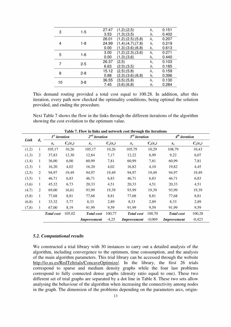
This demand routing provided a total cost equal to 100.28. In addition, after this
iteration, every path now checked the optimality conditions, being optimal the solution
provided, and ending the procedure.
Next Table 7 shows the flow in the links through the different iterations of the algorithm
showing the cost evolution to the optimum value.
Table 7. Flow in links and network cost through the iterations
Link de 1
st iteration 2
nd iteration 3
rd iteration 4
th iteration
xe Ce(xe) xe Ce(xe) xe Ce(xe) xe Ce(xe)
(1,2) 1 105,17 10,26 105,17 10,26 105,79 10,29 108,79 10,43
(1,3) 2 37,83 12,30 12,84 7,17 12,22 6,99 9,22 6,07
(1,4) 1 36,00 6,00 60,99 7,81 60,99 7,81 60,99 7,81
(2,3) 1 16,20 4,02 16,20 4,02 16,82 4,10 19,82 4,45
(2,5) 2 94,97 19,49 94,97 19,49 94,97 19,49 94,97 19,49
(3,5) 1 46,71 6,83 46,71 6,83 46,71 6,83 46,71 6,83
(3,6) 1 45,32 6,73 20,33 4,51 20,33 4,51 20,33 4,51
(4,7) 2 69,00 16,61 93,99 19,39 93,99 19,39 93,99 19,39
(5,8) 1 77,68 8,81 77,68 8,81 77,68 8,81 77,68 8,81
(6,8) 1 33,32 5,77 8,33 2,89 8,33 2,89 8,33 2,89
(7,8) 1 67,00 8,19 91,99 9,59 91,99 9,59 91,99 9,59
Total cost 105,02 Total cost 100,77 Total cost 100,70 Total cost 100,28
Improvement -4,25 Improvement -0,069 Improvement -0,423
5.2. Computational results
We constructed a trial library with 30 instances to carry out a detailed analysis of the
algorithm, including convergence to the optimum, time consumption, and the analysis
of the main algorithm parameters. This trial library can be accessed through the website
http://io.us.es/RedTeltrials/ConcaveOptimize/. In the library, the first 26 trials
correspond to sparse and medium density graphs while the four last problems
correspond to fully connected dense graphs (density ratio equal to one). These two
different set of trial graphs are separated by a dot line in Table 8. These two sets allow
analysing the behaviour of the algorithm when increasing the connectivity among nodes
in the graph. The dimension of the problems depending on the parameters arcs, origin-

14
2 � · � − 1��⁄
destination pairs, and number of paths communicating such pairs varies from around
500 constraints and 200 variables (instances 6 or 13) to more than 2,000 constraints and
1,000 variables (instances 1, 2 8, 16, 18, 29 or 30). This variety provides a good basis
for the analysis.
The considered parameters are detailed in Table 8. First, we included the number of
nodes, N, arcs, E, and origin-destination pairs, K. We have, also, analysed the volume of
demand in the network noted as kγ∑ , and the level of alternative paths forced in the
demand routing that we have called diversification and is given by kδ∑ (a lower result
from the sum requires a higher degree of alternative routing paths).
The main output values from our analysis are the cost, the algorithm computational time
and the required number of iterations, and they are compared with respect to the main
design parameter. The considered parameters were: (i) the number of nodes; (ii) the
number of arcs; (iii) the density of the graph that is calculated as the ratio between the
arcs and the maximum number of arcs considering possible connections among all the
nodes. So, the ratio is calculated as: ; (iv) the number of origin-
destination pairs; (v) the total demand volume in the network; and (vi) the
diversification parameter.
Table 8 provides the results obtained for the 30 instance library. Data related to the cost
and the required computational time and number of iterations to obtain the optimum are
provided together with data related to preparation of the problem. That is, the required
time for finding the paths in the graph connecting every origin-destination pair, as well
as the number of paths that was found.

15
Table 8. Summary of the trial library result
No.
Graph
Nodes
(N)
Arcs
(E) Density
Origin-destination
pairs (K) kγ∑ kδ∑
Pre-computing(1) Number of
iterations
Algorithm
time
(seconds)
Cost Time for
finding paths
Number of
paths
1 29 76 0.19 325 7500 243.60 0.093 8284 51 1415 2330.99
2 16 40 0.33 101 2470 74.52 0.015 653 19 52 867.90
3 17 44 0.32 134 2748 81.30 0.062 2832 20 128 929.25
4 28 64 0.17 349 6040 175.14 0.078 7221 23 1544 1976.86
5 24 65 0.24 235 5699 167.73 0.063 6290 42 756 1815.33
6 11 22 0.40 48 1184 37.31 0.063 171 8 11 363.51
7 21 49 0.23 165 3114 97.17 0.016 866 15 87 1163.39
8 26 65 0.20 284 5366 169.77 0.015 14950 34 2705 1846.75
9 10 14 0.31 37 671 22.44 0.001 91 2 1 274.93
10 19 47 0.27 162 4143 122.84 0.001 5442 19 215 1096.81
11 26 64 0.20 287 6984 217.22 0.079 15327 39 1312 2012.19
12 23 56 0.22 206 3915 125.53 0.001 3519 12 171 1236.76
13 18 31 0.20 137 2381 76.76 0.156 921 4 14 832.22
14 10 18 0.40 38 661 22.21 0.046 113 3 13 292.31
15 13 27 0.35 62 1440 47.23 0.047 227 5 11 559.51
16 30 73 0.17 346 6988 206.28 0.001 16882 28 2498 2284.20
17 14 28 0.31 66 1315 38.93 0.016 219 4 24 478.74
18 24 66 0.24 252 6353 179.64 0.001 18071 38 2767 1831.47
19 20 52 0.27 162 3597 100.10 0.001 2094 23 144 1148.47
20 21 56 0.27 173 3690 104.53 0.001 3050 22 160 1203.23
21 28 68 0.18 322 7438 244.62 0.094 6412 31 563 2337.84
22 15 37 0.35 94 1625 47.08 0.063 933 18 51 605.38
23 21 53 0.25 174 3890 128.89 0.063 3870 46 489 1270.06
24 17 37 0.27 111 2573 84.58 0.001 648 13 27 891.24
25 12 26 0.39 53 1069 31.22 0.001 181 7 28 448.28
26 15 31 0.30 78 1418 44.49 0.015 333 9 16 528.53
27 10 45 1.00 45 1099 44.01 0.005 1013 14 23 265.39
28 12 66 1.00 66 1695 64,01 0.005 4083 21 49 387.04
29 15 105 1.00 105 2638 103,01 0.005 32752 49 2890 618.72
30 16 120 1.00 120 3102 109 0.015 65519 51 3801 745.69 (1) See appendix 4
In next sections, we make a graphical analysis of the results in Table 8 (done in figures
2 to 6) in order to appreciate tendencies, dominances, etc. Firstly, we provide an
analysis for the set of sparse and medium density graphs, and secondly an analysis for
the four dense graphs is provided. The reason for separating them in the analysis is for
avoiding possible interferences between different conceptual graphs with a very
different density of arcs.
5.3. Analysis of the results for sparse and medium density graphs
First, we analyse tendencies and dependencies for sparse and medium density graphs.
Starting with the objective function dependencies with respect to the main parameters,
we can say that the cost of the problem maintains an approximately linear tendency with
respect to the number of nodes, the number of origin-destination pairs, the total demand
volume in the network, and the diversification parameter. On the other hand, the
relation with respect to the number of arcs in the graph slightly shows a higher than
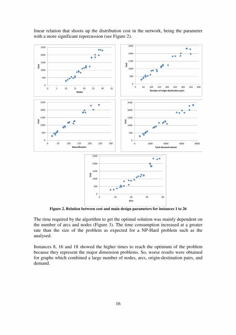
16
linear relation that shoots up the distribution cost in the network, being the parameter
with a more significant repercussion (see Figure 2).
Figure 2. Relation between cost and main design parameters for instances 1 to 26
The time required by the algorithm to get the optimal solution was mainly dependent on
the number of arcs and nodes (Figure 3). The time consumption increased at a greater
rate than the size of the problem as expected for a NP-Hard problem such as the
analysed.
Instances 8, 16 and 18 showed the higher times to reach the optimum of the problem
because they represent the major dimension problems. So, worse results were obtained
for graphs which combined a large number of nodes, arcs, origin-destination pairs, and
demand.
0
500
1000
1500
2000
2500
0 5 10 15 20 25 30 35
Co
st
Nodes
0
500
1000
1500
2000
2500
0 20 40 60 80
Co
st
Arcs
0
500
1000
1500
2000
2500
0 50 100 150 200 250 300 350 400
Co
st
Number of origin-destination pairs
0
500
1000
1500
2000
2500
0 2000 4000 6000 8000
Co
st
Total demand volume
0
500
1000
1500
2000
2500
0 50 100 150 200 250 300
Co
st
Diversification

17
Figure 3. Relation between computational time and main design parameters for instances 1 to 26
The number of iterations of the algorithm is strongly linked to the computational time of
the algorithm, and it is mainly affected by the density of the graph, as well as the
number of arcs and nodes too. So, the problems that take a greater time in the optimum
convergence were the larger problems and also those problems with a higher number of
pre-computed paths, which required a greater number of iterations (Table 8).
Following this later aspect, Figure 4 shows the relation between the number of paths
that were pre-computed for each graph, and the computational time and the number of
iterations of the algorithm. The figure shows that the increase in terms of computational
time and number of iterations follows an increasing tendency with a rate lower than
when it is analysed with respect to other design parameters (see how the increasing rate
is higher when the computational time is analysed with respect to other design
parameters in Figure 3). This fact contributes to validate and enhance the real potential
applicability of the approach.
0
500
1000
1500
2000
2500
3000
0 5 10 15 20 25 30 35
Tim
e
Nodes
0
500
1000
1500
2000
2500
3000
0 10 20 30 40 50 60 70 80
Tim
e
Arcs
0
500
1000
1500
2000
2500
3000
0 100 200 300 400
Tim
e
Number of origin-destination pairs
0
500
1000
1500
2000
2500
3000
0 1000 2000 3000 4000 5000 6000 7000 8000T
ime
Total demand volume
0
500
1000
1500
2000
2500
3000
0 50 100 150 200 250 300
Tim
e
Diversification
18
Figure 4. Time and number of iterations evolution with respect to the number of paths in the graph
for instances 1 to 26
Finally, Figure 5 provides an interesting analysis related to the algorithm convergence.
The optimising curve depicts a monotonic decrease of the total cost value that the
algorithm achieved, as shown in the figure. We have selected instances 1, 4, 8 and 18 as
representative examples to appreciate the algorithm convergence. It is interesting to
note how this phenomenon that is argued in appendix 3 is empirically checked when
solving the instances of the trial library.
Figure 5. Convergence to the optimum curves for graph instances 1, 4, 8 and 18
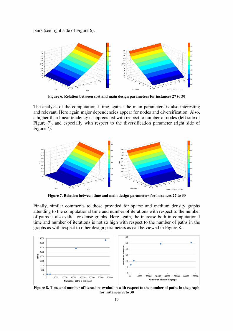
5.4. Analysis of the results for dense graphs
Finally, we analyse the main parameter dependencies related to dense graphs. Starting
with the objective function, the cost analysis in dense graph follows a very similar
structure to the analysis in sparse or medium density graphs, depicting a clearly linear
tendency. However, the linear dependency is stronger with respect to the nodes than the
arcs (see left side of Figure 6). Furthermore, the dependency with respect to the
diversification parameter ( kδ∑ ) than with respect to the number of origin-destination
0
500
1000
1500
2000
2500
3000
0 5000 10000 15000 20000
Tim
e
Number of paths in the graph
0
10
20
30
40
50
60
0 5000 10000 15000 20000
Nu
mb
er
of
ite
rati
on
s
Number of paths in the graph
2325,00
2330,00
2335,00
2340,00
2345,00
2350,00
2355,00
0 1 2 3 4 5 6 7 8 9 101112131415161718192021222324252627282930313233343536373839404142434445464748495051
CT
(to
tal co
st)
iterations
Graph #1
CT(Nº de Iteraciones)
1985,74
1985,57
1985,28
1983,231982,99
1981,03
1980,98
1980,21
1980,19
1980,14
1979,48
1979,47
1979,33
1979,28
1979,18
1978,96
1978,891978,59
1977,95
1977,00
1976,99
1976,93
1976,90
1976,86
1976,00
1977,00
1978,00
1979,00
1980,00
1981,00
1982,00
1983,00
1984,00
1985,00
1986,00
1987,00
0 1 2 3 4 5 6 7 8 9 10 11 12 13 14 15 16 17 18 19 20 21 22 23
CT(Total cost)
Iterations
Graph #4
CT(Nº de Iteraciones)
1844
1846
1848
1850
1852
1854
1856
1858
1860
1862
1864
1866
0 1 2 3 4 5 6 7 8 9 10 11 12 13 14 15 16 17 18 19 20 21 22 23 24 25 26 27 28 29 30 31 32 33 34
CT
(To
tal c
os
t)
Iterations
Graph #8
CT(Nº de Iteraciones)
483,07
482,12
479,65
479,05
478,74
478,50
479,00
479,50
480,00
480,50
481,00
481,50
482,00
482,50
483,00
483,50
0 1 2 3 4
CT
(To
tal c
os
t)
Iterations
Graph #18
CT(Nº de Iteraciones)
19
pairs (see right side of Figure 6).
Figure 6. Relation between cost and main design parameters for instances 27 to 30
The analysis of the computational time against the main parameters is also interesting
and relevant. Here again major dependencies appear for nodes and diversification. Also,
a higher than linear tendency is appreciated with respect to number of nodes (left side of
Figure 7), and especially with respect to the diversification parameter (right side of
Figure 7).
Figure 7. Relation between time and main design parameters for instances 27 to 30
Finally, similar comments to those provided for sparse and medium density graphs
attending to the computational time and number of iterations with respect to the number
of paths is also valid for dense graphs. Here again, the increase both in computational
time and number of iterations is not so high with respect to the number of paths in the
graphs as with respect to other design parameters as can be viewed in Figure 8.
Figure 8. Time and number of iterations evolution with respect to the number of paths in the graph
for instances 27to 30
0
500
1000
1500
2000
2500
3000
3500
4000
0 10000 20000 30000 40000 50000 60000 70000
Tim
e
Number of paths in the graph
0
10
20
30
40
50
60
0 10000 20000 30000 40000 50000 60000 70000
Nu
mb
er
of
ite
rati
on
s
Number of paths in the graph
20
6. Conclusions
In this paper we have proposed a novel optimal algorithm based on the Kuhn-Tucker
optimality conditions to determine the optimum of the demand routing problem in
multicommodity flow networks with diversification constraints and concave costs. The
aforementioned problem is considered NP-Hard because of its concave cost function. In
addition, it is an ambitious problem that takes most of the elements from traditional
concave cost transportation problems literature such as the objective function and the
multicommodity constraints, but also includes new elements as the diversification
constraints that have not been considered in concave cost paper literature, depicting a
more complex problem that those tackled in most of the concave cost transportation
papers. Such diversification constraints are required many times to model situations that
require diversifying elements in alternative routes of a distribution network, such as
freight in transportation networks or cells in telecommunication networks, modelling a
fact that appear in a number of real practice situations.
We have presented an iterative algorithm based on the Kuhn-Tucker optimality
conditions of the problem. Feasible solutions composed of an indicator path, a number
of ( )1 1k
δ − saturated paths and a set of empty paths are analysed for checking the
Kuhn-Tucker necessary conditions each iteration, since the sufficient condition is
always checked for every intermediate feasible solution defined as the previous one and
independently from its optimality. The algorithm enables the optimum to be reached
after a number of iterations. The method is a constructive step-by-step method because
after each iteration the total cost in the network is reduced in a monotonic sequence.
Therefore, given a MFDCC problem, a sufficiently high number of iterations of the
algorithm will allow reaching the optimum of the problem. It is clear that as the
MFDCC problem is NP-Hard, the number of iterations of the algorithm increases in a
non-polinomial way when the size of the problem increases. For very great size
problems this exact algorithm could not be efficient.
The algorithm showed a major dependency with respect to the number of nodes and
arcs of the problem as well as the level of diversification, which define the size of each
instance. Also the density of the graph depicted a clear influence for problems of the
same size increasing significantly the computational time. The number of origin-
destination pairs, as well as the number of alternative paths for connecting each origin-
destination pair revealed a not so relevant dependency levelling off its tendency. Also, it
is relevant to note that tendencies were appreciated in a similar way both for sparse,
medium density and dense graphs.
The optimum was obtained for all the instances studied, and the time consumption was
feasible when analysed from a non-real-time perspective, which is normal in network
design problems. Although in real time situations, the algorithm may not be suitable
depending on the time response required, alternatives such as stop criteria after a
number of iterations or time consumption could be considered because the method
guarantees a monotonic approach to the optimum.
21
Acknowledgements
The authors acknowledge an anonymous referee for his/her helpful comments on earlier
versions of this manuscript that have significantly contributed to enrich the quality of
the paper in its final form.
Appendix 1
Appendix 1 states the Kuhn-Tucker optimality necessary conditions for every
optimisation problem, and its application to the MFDCC problem.
Consider the next generic optimization problem:
The Kuhn-Tucker conditions are given by:
The Kuhn-Tucker conditions for the MFDCC problem are given by:
A solution verifying the necessary condition is only optimum if it verifies also the
sufficiency condition in problems with non-convex objective functions.
Appendix 2
Appendix 2 deals with the Kuhn-Tucker optimality sufficient conditions. In addition,
here is proven that every solution for the communication of K commodities, each of
them with a demand γk and forced to a diversification given by δk, that is composed by a
set of ( )1 1k
δ − saturated paths, an indicator path and being the rest void paths verifies
the Kuhn-Tucker sufficient conditions. Thus, every solution associated to each iteration
of the algorithm described in section 4 will verify the Kuhn-Tucker sufficient condition.
��� � �� (13)
s.t.: �� �� ≤ 0 , ∀� (14) ℎ� �� = 0 , ∀� (15) � ∈ ℛ�
∇� �� + # $� ∇�� �� +� # %�∇ℎ� ��� = 0
(16)
�� �� ≤ 0 , ∀� ℎ� �� = 0 , ∀� (17) $� · �� �� = 0 , ∀� (18) $� ≥ 0 ∀� and %� �*++ (19)
,- .�,.�ℎ − %� = $�ℎ − /�ℎ (20)
.�ℎ − 0� · 1� � · /�ℎ = 0 (21) .�ℎ · $�ℎ = 0 (22) $�ℎ , /�ℎ ≥ 0 and %� �*++ (23)
22
2ℎ3′ > 2ℎ�′
Let consider the generic problem given by equations (13-15). The sufficiency condition
for such generic problem is given by (24):
Where:
The sufficiency condition for the MFDCC problem is given by (25):
And this expression must be satisfied in set V(x) that is defined as:
Therefore, any flow pattern verifying equations (20 to 23) verifies the sufficient
condition too, and therefore the necessary conditions becomes the global optimality
conditions for the specific structure of the analysed problem.
Appendix 3
Appendix 3 proves that the algorithm described in section 4, guarantees the reduction of
the cost of the objective function after each step following a monotonic sequence to
optimality.
Suppose that after iterating, the Kuhn-Tucker conditions cannot be satisfied for every
origin-destination pairs. Therefore, the origin-destination pair k* is given by (9). For
such pair three options can appear:
a) the derivative is higher in a saturated path than in the indicator path
67∇�� 8 �, $, %�6 ≥ 0 ∀6 ∈ 9 �� (24)
∇� 8 �, $, %� = ∇� �� + # $� ∇�� �� +� # %�∇ℎ� ���
and: 9 �� = �6 ∈ ℛ� : ∇ℎ� ��7 · 6 = 0 , ∀� ; ∇�� ��7 · 6 = 0 , ∀� ∈ ���
where A(x) is the set of active constraints (that is, verifies constraint �� �� ≤ 0 with
zero slack).
67 <,2- .�,.�ℎ2 = 6 ≥ 0, ∀6 ∈ 9 �� (25)
9 �� = >6 ∈ ℛ� : # 6�ℎ = 0, ∀� ∈ �ℎ∈? �� and 6�ℎ = 0 for those paths ℎ ∈ ? �� so that .�ℎ= 0� saturated paths�or so that .�ℎ = 0 empty paths�K
which is verified by every feasible solution associated to the corresponding iteration of
the algorithm described in section 4. In effect, equation (25) is verified in every
saturated and empty path because 6�ℎ = 0 for such paths, and the indicator path verifies
also 6�ℎ = 0 because ∑ 6�ℎ = 0, ∀� ∈ �ℎ∈? �� and there is only one indicator path in
each iteration, so being the other paths (saturated and empty) equal to zero, the indicator
path must be equal to zero too.
23
2ℎ�′ > 2ℎ/′ 2ℎ3′ − 2ℎ�′ � and 2ℎ �′ − 2ℎ/′ �
2ℎ3′ − 2ℎ�′ � > 2ℎ�′ − 2ℎ/′ �.
2ℎ3′ − 2ℎ�′ � < 2ℎ�′ − 2ℎ/′ �.
b) the derivative is higher in the indicator path than in a void path
c) Both situations occur but one of the expressions: is
higher than the other, so we select the corresponding case.
So we need to analyse the recirculation of flow for the two cases given below as option
A and option B.
Option A:
It corresponds to recirculate the flow from the saturated path to the indicator path for
cases a) or c) when
Total cost is given for current situation (26) and, after recirculating, new situation (27):
So, there is an unchanging part given by the flown on the links for every link not
belonging to the saturated or indicator path, and a changing part given by the links in
the saturated and indicator paths.
Calculating the variation of cost between new and current situations, equation (28) is
reached.
Option B
It corresponds to recirculate the flow from the indicator path to the void path for cases
b) or c) when
Total cost is given for current situation (29) and, after recirculating, new situation (30):
-2 ?� = # 2+ �+ �+∉�ℎ3 ;ℎ�� + # 2+ �+ �+∈ℎ3+ # 2+ �+ �+∈ℎ�
(26)
-� ?� = # 2+ �+ �+∉�ℎ3;ℎ�� + # 2+ �+ −△ ��+∈ℎ3+ # 2+ �+ +△ ��+∈ℎ�
(27)
-� ?� − -2 ?� = O # 2+ �+ �+∈ℎ3
+ # 2+ �+ −△ ��+∈ℎ3
P + O# 2+ �+ �+∈ℎ�
+ # 2+ �+ +△ ��+∈ℎ�
P (28)
From the checking of the Kuhn-Tucker conditions we know that 2ℎ3′ > 2ℎ�′ (that was the
reason for non-optimality). Therefore, the decrease in the cost experimented when
reducing flow in the saturated path corresponding to the evaluation of the first term of
the sum is higher than the increase in the cost experimented when increasing flow in the
indicator path corresponding to the evaluation of the second term of the sum (this
argument is based on 2ℎ3′ > 2ℎ�′ ). And thus, -� ?� − -2 ?� < 0 producing a decrease of the
total cost after recirculating the flow consequently.
-2$**+�R ?� = # 2+ �+ �+∉�ℎ� ;ℎ/� + # 2+ �+ �+∈ℎ�+ # 2+ �+ �+∈ℎ/
(29)
24
So, there is an unchanging part given by the flown on the links for every link not
belonging to the indicator or void path, and a changing part given by the links in the
indicator and void paths.
Calculating the variation of cost between new and current situations, equation (31) is
reached.
These arguments prove that after each iteration the total cost in the network is reduced.
Therefore, given a MFDCC problem, a sufficiently high number of iterations of the
algorithm allow reaching the optimum of the problem. It is clear that as this problem is
NP-Hard, the number of iterations of the algorithm increases in a non-polinomial way
when the size of the problem increases.
Appendix 4
This appendix includes the procedure followed to find all the paths in a graph. There are
several alternatives to find all the paths between a pair of nodes in a graph. Most of
them follow Depth-First Search (DFS) or Breadth-First-Search (BFS) structures. We
followed a procedure based in the DFS algorithm. This is a well-known algorithm that
can be described as next:
Input: A graph G and a vertex v of G
Output: A labelling of the edges in the connected component of v as
discovery edges and back edges
procedure DFS(G,v):
label v as explored
for all edges e in G.adjacentEdges(v) do
if edge e is unexplored then
w ← G.adjacentVertex(v,e)
if vertex w is unexplored then
label e as a discovery edge
recursively call DFS(G,w)
-�+S ?� = # 2+ �+ �+∉�ℎ� ;ℎ/� + # 2+ �+ −△ ��+∈ℎ�+ # 2+ �+ +△ ��+∈ℎ/
(30)
-� ?� − -2 ?� = O# 2+ �+ �+∈ℎ�
+ # 2+ �+ −△ ��+∈ℎ�
P + O # 2+ �+ �+∈ℎ/
+ # 2+ �+ +△ ��+∈ℎ/
P
(31)
From the checking of the Kuhn-Tucker conditions we know that 2ℎ�′ > 2ℎ/′ (that was the
reason for non-optimality). Therefore, the decrease in the cost experimented when
reducing flow in the indicator path corresponding to the evaluation of the first term of
the sum is higher than the increase in the cost experimented when increasing flow in the
void path corresponding to the evaluation of the second term of the sum (this argument
is based on 2ℎ�′ > 2ℎ/′ ). And thus, -� ?� − -2 ?� < 0 producing a decrease of the total cost
after recirculating the flow consequently.

25
else
label e as a back edge
References
1. Altiparmak F, Dengiz B, Smith AE., 2003. Optimal design of reliable computer
networks: A comparison of metaheuristics. Journal of Heuristics 9, 471-487.
2. Altiparmak F, Karaoglan I., 2008. An adaptive tabu-simulated annealing for concave
cost transportation problems. Journal of the Operational Research Society 59, 331-341.
3. Avriel, M., 2003. Nonlinear Programming: Analysis and Methods. Dover Publishing.
4. Burkard RE, Dollani H, Thach PT., 2001. Linear approximations in a dynamic
programming approach for the uncapacitated single source minimum concave cost
network flow problem in acyclic networks. Journal of Global Optimization 19, 121-139.
5. Dengiz B, Altiparmak F, Smith AE., 1997. Local search genetic algorithm for
optimal design of reliable networks. IEEE Transactions on Evolutionary Computation 1;
179–188.
6. Cortes, P., Muñuzuri, J., Onieva, L., Larrañeta, J., Vozmediano, J.M., Alarcon, J.C.,
2006. Andalucía assesses the investment needed to deploy a fiber-optic network.
Interfaces 36 (2), 105-117
7. Florian M, Klein M., 1971. Deterministic production planning with concave cost and
capacity constraints. Journal of Management Science 18, 12–20.
8. Hanson MA, Mond B., 1987. Necessary and sufficient conditions in constrained
optimization. Mathematical programming 37; 51-58.
9. Hillier, F.S., Lieberman, G.J., 1974. Operations Research. Holden-Day Inc. (San
Francisco, California, US)
10. Hitchcock, F.L., 1941. The distribution of a product from several sources to
numerous locations. Journal of Mathematical Physics 20, 224–230.
11. Kapsalis A, Rayward-Smith VJ, Smith GD., 1993. Solving the graphical Steiner tree
problem using genetic algorithms. Journal of the Operational Research Society 44, 397–
406.
12. Kengpol, A., Meethom, W., Tuominen, M., 2012. The development of a decision
support system in multimodal transportation routing within Greater Mekong sub-region
countries. International Journal of Production Economics 140(2), 691–701.
13. Kleinberg, J. 1996. Approximation Algorithms for Disjoint Paths Problems. Ph.D
Thesis, Department of EECS, MIT.
26
14. Larsson T, Migdalas A, Ronnqvist M., 1994. A lagrangian heuristic for the
capacitated concave minimum cost network flow problem. European Journal of
Operational Research 78, 116–129.
15. LeBlanc, L.J., 1976. Global solutions for a nonconvex, nonconcave rail network
model. Management Science 23, 131-139.
16. Nocedal, J., Wright, S. J., 2006. Numerical Optimization (Second Edition) by
Numerical Optimization, Springer.
17. Thach PT., 1992. A decomposition method using a pricing mechanism for minimum
concave cost flow problems with a hierarchical structure. Journal of Mathematical
Programming 53, 339–359.
18. Tsao, Y-C., Sheen, G-J., 2012. A multi-item supply chain with credit periods and
weight freight cost discounts. International Journal of Production Economics 135 (1),
106-115.
19. Ubeda, S., Arcelus, F.J., Faulin, J., 2011. Green logistics at Eroski: A case study.
International Journal of Production Economics 131(1), 44-51.
20. Yan S, Luo SC., 1999. Probabilistic local search algorithms for concave cost
transportation network problems. European Journal of Operational Research 117, 511–
521.
21. Zangwill WI., 1968. Minimum concave cost flows in certain networks. Management
Science 14, 429–450.
22. Zhou G, Gen M., 2003. A genetic algorithm approach on tree like
telecommunication network design problem. Journal of the Operational Research
Society 54, 248-254.


