
NASA / CR-1998-208721
Operational Data Reduction Procedure for
Determining Density and Vertical Structure of
the Martian Upper Atmosphere From Mars
Global Surveyor Accelerometer Measurements
George J. Cancro, Robert H. Tolson, and Gerald M. Keating
The George Washington University
Joint Institute for Advancement of Flight Sciences
Langley Research Center, Hampton, Virginia
National Aeronautics and
Space Administration
Langley Research CenterHampton, Virginia 23681-2199
Prepared for Langley Research Center
under Cooperative Agreement NCCI-104
October 1998
https://ntrs.nasa.gov/search.jsp?R=19990005111 2018-07-10T20:04:08+00:00Z

Available from the following:
NASA Center for AeroSpace Information (CASI)7121 Standard Drive
Hanover, MD 21076-1320
(301) 621-0390
National Technical Information Service (NTIS)
5285 Port Royal Road
Springfield, VA 22161-2171(703) 487-4650
-q |F

Abstract
The success of aerobraking at Mars by the Mars Global Surveyor (MGS)
spacecraft was partly due to the analysis of MGS accelerometer data. Accelerometer data
was used to determine the effect of the atmosphere on each orbit, to characterize the
nature of the atmosphere, and to predict the atmosphere for future orbits. To properly
interpret the accelerometer data, a data reduction procedure was developed which utilizes
inputs from the spacecraft, the MGS Navigation Team, and pre-mission
aerothermodynamic studies to produce density estimations at various points and altitudes
on the planet. This data reduction procedure was based on the calculation of acceleration
due to aerodynamic forces from the accelerometer data by considering acceleration
components due to gravity gradient, solar pressure, angular motion of the instrument,
instrument bias, thruster activity, and a vibration component due to the motion of the
damaged solar array. Methods were developed to calculate all of the acceleration
components including a 4 degree of freedom dynamics model used to gain a greater
understanding of the damaged solar array. An iteration process was developed to
calculate density by calculating deflection of the damaged array and a variable force
coefficient. The total error inherent to the data reduction procedure was calculated as a
function of altitude and density considering contributions from ephemeris errors, errors in
force coefficient, and instrument errors due to bias and digitization. Comparing the results
from this procedure to the data of other MGS Teams has demonstrated that this procedure
can quickly and accurately describe the density and vertical structure of the Martian upper
atmosphere.

-7 I I-

Table of Contents
Abstract ........................................................................................................................... i
Table of Contents .......................................................................................................... iii
List of Figures ................................................................................................................ v
List of Tables ............................................................................................................... vii
Nomenclature .............................................................................................................. viii
1. Introduction ............................................................................................................... 1
2. MGS Aerobraking Scenario ...................................................................................... 3
2.1 Accelerometer Instrument .......................... ............................................................. 3
2.2 MGS Aerobraking Configuration ............................................................................ 3
2.3 Complexities of the MGS Aerobraking Mission ...................................................... 4
2.4 Accelerometer Team Responsibilities ...................................................................... 6
2.5 Description of Panel Malfunction ............................................................................ 8
3. Analysis of Acceleration Data ................................................................................. 10
3.1 Development of the Acceleration Term ................................................................. 10
3.2 Development of the Spacecraft Velocity Term ...................................................... 21
3.3 Development of the Ballistic Coefficient Term ...................................................... 22
4. Operational Data Reduction Procedure ................................................................. 28
4.1 Operational Constraints ........................................................................................ 28
4.2 Operational Accelerometer Instrument .................................................................. 29
4.3 Quantity of Accelerometer Data Necessary to Perform Operations ........................ 31
4.4 Operational Data Reduction Process ..................................................................... 34
4.5 Special Products ................................................................................................... 40
4.6 Prediction Methods ............................................................................................... 43
5. Analysis of Process Errors ......................................... i............................................. 45
5.1 Ephemeris Errors .................................................................................................. 45
5.2 Errors in Determining Ballistic Coefficient ............................................................ 46
5.3 Errors in Determining Bias .................................................................................... 47
iii

5.4 Errors due to Instrument Output ........................................................................... 48
5.5 Total Data Reduction Process Error ..................................................................... 49
6. Verification of Accelerometer Results ..................................................................... 51
6.1 Data Reduction Process Verification ..................................................................... 51
6.2 Prediction Scheme Verification ............................................................................. 54
7. The Effect of Panel Vibration on MGS and the Accelerometer Data Reduction
Process .......................................................................................................................... 57
7.1 Effectiveness of the 4 DOF Dynamics Model ........................................................ 58
7.2 Verification of the Dynamics Model And Assumptions .......................................... 59
7.3 Sensitivity Studies on Panel Physical Parameters ................................................... 61
7.4 Averaging Techniques Used to Compensate for Vibrating Panel Effects ................ 64
8. Conclusions .............................................................................................................. 65
References .................................................................................................................... 67
APPENDIX A: Description of Quick-Look Data Product ......................................... 69
APPENDIX B: 4 DOF Derivation for Eliminating SAM panel Motions from Z-
Accelerometer Data ........................................................................... 74
APPENDIX C: LaRC Aerothermodynamic Database for MGS Operations ............ 80
APPENDIX D: Planetary Ephemeris and Physical Data ........................................... 89
APPENDIX E: MGS Physical Properties ................................................................... 90
APPENDIX F: Verification of 4 DOF Model Derivation ........................................... 91
iv
;1 1I !

List of Figures
Figure 2-1 :
Figure 2-2:
Figure 2-3:
Figure 3-1:
Figure 3-2:
Figure 3-3:
Figure 3-4:
Figure 3-5:
Figure 3-6:
Figure 3-7:
Figure 3-8:
Figure 3-9:
Figure 3-10:
Figure 4-1:
Figure 4-2:
Figure 4-3:
Figure 4-4:
Figure 4-5:
Figure 4-6:
Figure 4-7:
Figure 4-8:
Figure 4-9:
Figure 5-1 :
MGS aerobraking configuration ................................................................... 4
Diagram of basic MGS project team relationships ........................................ 7
Spare yoke with suspected failure mode ....................................................... 9
Typical spacecraft angular rates (Orbit 162) ............................................... 16
Typical x, y and z angular accelerations (Orbit 162) ................................... 16
Typical thruster fire times (Orbit 16) .......................................................... 18
Acceleration data with large amplitude vibrations (Orbit 95) ...................... 19
Diagram of 2-body 4 DOF model used to estimate moving panel
acceleration ................................. . ............................................................ 19
Ux and Uy coordinate definition ................................................................ 23
Force coefficient in spacecraft z-direction, Cz, vs. density level for all
panel deflections ....................................................................................... 24
Cz tables for free molecular densities (0 degree SAM Deflection and 10
degree SAM Deflection) ........................................................................... 25
Typical quaternions (Orbit 162) ................................................................. 26
Typical Ux and Uy diagram (Orbit 162) ..................................................... 27
Typical IMU temperatures and voltage to IMU heater (Orbit 162) ............. 30
Results of Accelerometer Data Rate Simulation ......................................... 32
Results of accelerometer data rate simulation considering all possible
outcomes .................................................................................................. 33
Data reduction process flow chart .............................................................. 34
Typical accelerometer instrument bias calculation ...................................... 36
Development of density flow chart ............................................................. 37
Typical z-force coefficient and panel deflection from Orbit 162 .................. 38
Comparison of the operational averaging techniques .................................. 39
Look-ahead model diagram ........................................................................ 44
Accelerometer process error vs. model altitude and density ....................... 50
V

Figure 6-1 :
Figure 6-2:
Figure 6-3:
Figure 7-1 :
Figure 7-2:
Figure 7-3:
Figure 7-4:
Figure 7-5:
Figure 7-6:
Figure 7-7:
Comparison of panel position calculated using accelerometer data and sun
sensor data ................................................................................................. 52
Orbital decay comparison of NAV and ACC using p_s product .............. 53
Comparison of effectiveness of persistence, 5-orbit mean, longitudinal
wave, and look ahead prediction schemes over Orbits 100-200 .................. 55
Acceleration profiles for Orbit 162 - raw data, reduced data using
4 DOF model, and reduced data using band-pass filtering method .............. 58
Acceleration profiles for Orbit 95 - raw data, reduced data using
4 DOF model, and reduced data using band-pass filtering method .............. 59
Sensitivity study on SAM moment of inertia about the spacecraft
x-axis at the SAM center of mass ...................................................... ......... 62
Sensitivity study on SAM mass ................................................................... 62
Sensitivity study on SAM center of gravity position .................................... 63
Sensitivity study on crack-line position ........................................................ 63
Comparision between 4 DOF dynamics model and 40 pt (left) and
6 pt running means (right) for Orbit 162 ..................................................... 64
vi
I-1 1-

List of Tables
Table 3-1:
Table 3-2:
Table 3-3:
Table 4- l :
Table 4-2:
Table 5-1:
Table 5-2:
Table 5-3:
Table 54:
Table 5-5:
Table 6-1:
Table 7-1:
Aerodynamic Force Acceleration Simulation Results .................................... l 1
Gravity Gradient Acceleration Simulation Results ........................................ 13
Results of Range Error Study Between Exact Ephemeris and Ephemeris
Generated From Osculating Elements at Periapsis ........................................ 22
Telemetry Data Types And Rates For Operations ......................................... 29
Results From Reliability of Accelerometer Data Simulation .......................... 33
Total Altitude Error Results ......................................................................... 46
Ephemeris Timing Error Results for 0.1 Seconds of Timing Error ................ 46
Bias Percent Error as a Function of Count Level .......................................... 48
Quantization and Data Rate Error Results .................................................... 48
Total Data Reduction Process Error ............................................................. 49
Results of NAV Simulation Runs with Accelerometer Calculated
Effective Scale Height ................................................................................. 54
Crack-Line Position and Resulting Physical Parameters
for Sensitivity Study .................................................................................... 61
vii

Nomenclature
_c
A
ACC
ADL
a,e,i,w,f2,x
az
azBp
BUS
Cl, C2
Cx Cy Cz
CMx CMy CMz
C
5_
15_c
DCM
DOF
AR
At, A0, Az
ETC
F,
f
fm
g
HGA
= right ascension of the sun in Mars equatorial coordinates, rad
= right ascension of the spacecraft in Mars equatorial coordinates, rad
= angular acceleration of the spacecraft, rad/s 2
= spacecraft reference area, 17.03 m 2
= Accelerometer
= Atmospheric Disturbance Level
= Keplerian orbital elements: semi-major axis, eccentricity, inclination,
argument of periapsis, longitude of ascer_ding node, time of periapsis
= acceleration due to aerodynamic forces in spacecraft z-axis, m/s:
= band-pass filtered z-axis acceleration, m/s z
= spacecraft main body
= parameters of band-pass filter
= force coefficients in the spacecraft x, y, z axes, respectively
= moment coefficients about the spacecraft x, y, z axes, respectively
= speed of light, 3"108 m/s
= declination of the sun in Mars equatorial coordinates, rad
= declination of the spacecraft in Mars equatorial coordinates, rad
= Direction Cosine Matrix
= Degrees Of Freedom
= areocentric distance to accelerometer instrument, km
!
= cylindrical components of AR
= Ephemeris Timing Correction
= solar constant, 590 W/m 2 at Mars
= true anomaly
= flattening of Mars
= acceleration of gravity on Mars surface, 3.4755 m/s 2
= High Gain Antenna
.o.VIII
:1 I I

Us
h
IMU
L
L
LMA
LST
B
m
MGS
NAV
CO
P
po
Q
q
q_
ql, q2, q3, q4
i
R
_m
R,O,Z
rcm
SAM
SAP
SZA
S/C
05
= scale height, km
= angular momentum of an orbit, km2/s
= Inertial Measurement Unit
= longitude, deg
= rotation rate of Mars, deg/day
= Lockheed Martin Astronautics
= Local Solar Time, Martian hrs
= gravitational constant for Mars, 42828 km3/s 2
= spacecraft mass, kg
= Mars Global Surveyor
= Navigation
= angular velocity of the spacecraft, rad/s
= density, kg/km 3
= base density, kg]km 3
= free stream heat flux, W/cm 2
= dynamic pressure, N/m 2
= reflectance factor for solar pressure
= spacecraft quaternions
= areocentric distance to accelerometer instrument, km
= areocentric distance to spacecraft center of mass, km
= cylindrical orbit coordinates: distance from planet, angular distance
along orbit path, distance perpindicular to orbit path
= radial distance from Mars center to spacecraft center of mass, km
= Solar Array Minus (on -Y spacecraft axis)
= Solar Array Plus (on +Y spacecraft axis)
= Solar Zenith Angle, deg
= Spacecraft
= angular velocity in orbit plane, deg/s
= deflection angle of the damaged solar array, deg
ix

Oi
OL
OL'
T
To
T:
TCM
Ux ,Uy
V
Z
Zo
= Incidence angle of solar radiation, deg
= areocentric latitude, deg
= areodetic latitude, deg
= spring torque, in-lbs
= base temperature, K
= temperature change with altitude, K/km
= Trajectory Correction Maneuver
= direction sines describing the orientation of the relative wind with
respect to the spacecraft x and y axes
= orbital velocity of spacecraft, krn/s
= areodetic altitude, km
= base altitude, km
X
1. Introduction
The Mars Global Surveyor (MGS) spacecraft is NASA's first orbiter to return to
the red planet in 20 years. MGS represents the first project in the NASA Mars Surveyor
Program, a series of missions to Mars every 25 months over a period of 10 years. The
goals of the Mars Surveyor Program are to analyze the physical and atmospheric
properties of the planet and gain a greater understanding of how Mars formed [ 1]. The
MGS mission begins this analysis by achieving the following science goals:
(1) Successfully characterize the gravity field and surface properties of the planet,
(2) Establish the nature of the magnetic field, and
(3) Monitor the global structure of the atmosphere [2].
To accomplish these goals while maintaining a low budget, a technique called
"aerobraking" was planned to position the MGS spacecraft close enough to the planet for
onboard science instruments to properly collect data. Aerobraking is the process of using
atmospheric drag to remove kinetic energy from an orbit. The MGS spacecraft used
repeated encounters with the atmosphere (aerobraking passes) to gradually change a long
period-high eccentricity orbit to a short period-low eccentricity orbit. By relying on
multiple aerobraking passes instead of propulsive maneuvers to modify the orbit, less fuel
was needed during the MGS mission and, therefore, the design weight of the spacecraft
was reduced.
Aerobraking had to be monitored during each pass through the atmosphere to
ensure the safety of the spacecraft and the effectiveness of the technique. To monitor
aerobraking, Keating et al. [Keating, G.M., Tolson, R.H., Bougher S.W., Blanchard R.C.,
"MGS Accelerometer Proposal for JPL Operations, Dec 1995. Available from author]
proposed the use of on-board accelerometer data to produce density estimations as a
function of altitude for each pass and density predictions for future passes. In accord with
this proposal, a data reduction procedure was created. This paper presents the data
reduction procedure and demonstrates the effectiveness of this procedure in calculating

andpredictingdensitiesfor 149aerobrakingorbits completed by MGS. Th_se 149 orbits
occurred during the first 201 orbits at Mars, called the 1st phase of aerobr,:_:!ag.
First, this paper discusses the MGS aerobraking scenario including descriptions of
the accelerometers, the MGS spacecraft and the malfunction of one of the solar arrays on
the spacecraft. Next, the relationship betwee _ atmospheric density and acceleration due to
aerodynamic forces is examined. Methods ,_'_ _":developed to determine each of the
components of this relationship. One such method is a dynamics model designed to
compensate for the effects of the damaged solar array on the measured acceleration.
These methods are combined with an iterative process to form the data reduction
procedure which determines density from accelerometer data. The errors inherent to the
data reduction procedure are calculated by considering ephemeris errors, force coefficient
errors, and instrument errors. The data reduction procedure is verified using panel
deflection data determined by the MGS Spacecraft Team and orbital period reduction data
generated by the MGS Navigation Team.
Finally, the methods developed in this report are used to give a greater insight into
the solar array malfunction. The dynamics model mentioned briefly above, successfully
compensates for 90% of vibration signal associated with the solar array malfunction.
Sensitivity studies were performed using the dynamics model to determine the source of
the remaining 10%.
I-I1-

2. MGS Aerobraking Scenario
This section will describe the key elements of the MGS aerobraking scenario
including the accelerometer instrument, the aerobraking configuration, the complexities of
aerobraking at Mars, and the role of the team monitoring the aerobraking process using
on-board accelerometer data.
During deployment, one of the two solar arrays on the MGS spacecraft
malfunctioned. This section also gives a brief description of this malfunction and how the
malfunction effects the analysis of accelerometer data.
2.1 Accelerometer Instrument
The MGS accelerometers are instruments that measure the change in velocity of
the spacecraft over a time interval by measuring the fluctuations of voltage to an
electromagnetic assembly. The assembly is essentially a magnetic proof mass suspended
on a thin flexure in an electromagnetically charged ring. When the spacecraft accelerates,
the position of the proof mass inside the ring is maintained by varying the voltage. After
the instrument is calibrated in a known g-field, the acceleration of the spacecraft can be
calculated by recording the change in voltage to the ring.
2.2 MGS Aerobraking Configuration
Several minutes before beginning the aerobraking pass through the Martian
atmosphere, the MGS spacecraft was placed in the aerobraking configuration. The
aerobraking configuration, shown in Figure 2-1, consists of the spacecraft oriented with
the main engine nozzle (spacecraft -z axis) pointed in the direction of spacecraft motion or
the "velocity vector" and the High Gain Antenna (spacecraft x axis) pointed toward the
planet,"nadir", or away from the planet,"zenith". The two solar arrays, solar array plus

(SAP)andsolararrayminus(SAM),extendfrom the+Y and-Y facesof themainbody,
or "BUS", respectively.Thesolararraysconsistof two separatepanels(innerandouter)
andarecomposedof carbon-carboncompositefacesheetsoverhoneycombcore. Gallium
arsenideandsiliconsolarcellscoveronly onefaceof thesearrays.Duringaerobraking,
themajority of theatmosphericdragon thespacecraftwasproducedby thesesolararrays
whichwereplannedto beorientedwith thenon-cellfaceinto thewind andsweptback30
degreesfor aerodynamicstability.Thefour accelerometersusedduringaerobrakingare
containedwith four gyrosinsidetheInertialMeasurementUnit (IMU). TheIMU is
locatedon thetopdeckof theBUS alongwith theotherMGS scienceinstruments.
SAM Z
(Broken Panel)
Sun Sensor--/ i ___
Yoke Crac_
ACS Pod - 3 Jets / _ --
Cryp. of 4)
SAP
_r Panelt
__ High Gain _Y
'_X Antenna
Nominal WindDirection
Figure 2-I: MGS aerobraking configuration
2.3 Complexities of the MGS Aerobraking Mission
Aerobraking is not a new technique. Planetary aerobraking was used at Venus
during the Magellan mission to circularize the orbit [3] and used again in the Termination
Experiment to study the Venusian atmosphere and improve the estimates of the
aerodynamic properties of the Magellan spacecraft [4].
Ill
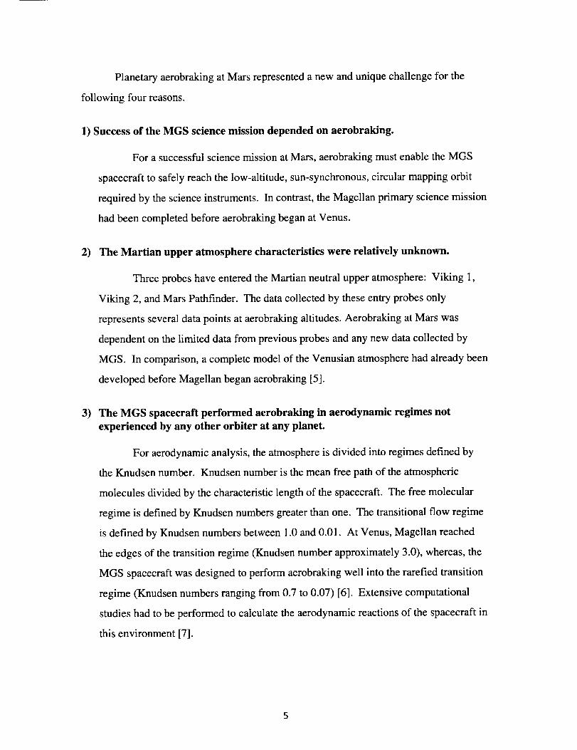
Planetary aerobraking at Mars represented a new and unique challenge for the
following four reasons.
1) Success of the MGS science mission depended on aerobraking.
For a successful science mission at Mars, aerobraking must enable the MGS
spacecraft to safely reach the low-altitude, sun-synchronous, circular mapping orbit
required by the science instruments. In contrast, the Magellan primary science mission
had been completed before aerobraking began at Venus.
2) The Martian upper atmosphere characteristics were relatively unknown.
Three probes have entered the Martian neutral upper atmosphere" Viking 1,
Viking 2, and Mars Pathfinder. The data collected by these entry probes only
represents several data points at aerobraking altitudes. Aerobraking at Mars was
dependent on the limited data from previous probes and any new data collected by
MGS. In comparison, a complete model of the Venusian atmosphere had already been
developed before Magellan began aerobraking [5].
3) The MGS spacecraft performed aerobraking in aerodynamic regimes not
experienced by any other orbiter at any planet.
For aerodynamic analysis, the atmosphere is divided into regimes defined by
the Knudsen number. Knudsen number is the mean free path of the atmospheric
molecules divided by the characteristic length of the spacecraft. The free molecular
regime is defined by Knudsen numbers greater than one. The transitional flow regime
is defined by Knudsen numbers between 1.0 and 0.01. At Venus, Magellan reached
the edges of the transition regime (Knudsen number approximately 3.0), whereas, the
MGS spacecraft was designed to perform aerobraking well into the rarefied transition
regime (Knudsen numbers ranging from 0.7 to 0.07) [6]. Extensive computational
studies had to be performed to calculate the aerodynamic reactions of the spacecraft in
this environment [7].

4) The density of the Martian atmosphere can increase rapidly due to dust storms
The MGS spacecraft arrived at Mars during southern hemisphere spring, near the
time when dust storms are most likely to form on the planet [8]. These storms raise the
temperature of the lower atmosphere, thereby, expanding the upper atmosphere. If the
MGS spacecraft unknowingly encountered such a expansion, the atmosphere could
overheat the solar arrays on the spacecraft.
2.4 Accelerometer Team Responsibilities
To compensate for the complexities above, the Accelerometer (ACC) Team was
formed from senior personnel and graduate students of the George Washington University
at NASA Langley. Using inputs from the MGS spacecraft and the MGS Navigation
(NAV) Team, the ACC Team was assigned to support the aerobraking process by:
1) Producing atmospheric structure information on each aerobraking pass,
2) Supporting the NAV Team by providing density and density scale height
information, and
3) Providing predictions of density on future aerobraking passes.
By producing atmospheric structure information for each pass, the ACC Team provided
critical results concerning the upper atmosphere to the Atmospheric Advisory Group
(AAG), which was responsible for monitoring the entire atmosphere on Mars. The ACC
Team also supported the NAV Team, responsible for orbit determination, by providing
density at periapsis and a scale height used to determine the orbit during the aerobraking
pass. Scale height is the altitude increase over which the density decreases by a factor of
e. Finally, by providing predictions of density on future aerobraking passes, the ACC
Team assisted the MGS project to plan future passes and ensure the safety of the
spacecraft.
To accomplish these tasks, a procedure was developed for determining several
atmospheric properties including density, scale height, pressure, temperature, dynamic
-q |1-

pressure and free-stream heatflux for each aerobraking pass. The procedure was
separated into two steps: Accelerometer Data Reduction and Atmospheric Data Modeling
as shown in Figure 2-2 below.
/LTelemetry_ Accelerometer I Effective
Data Reduction I Scale Height
Procedure I !Densi_J vs. r t_1Predictions
/I
I
Orbit_Path _ I
Atmospheric_
Data Modeling j
PredictionMethods
MOSt Project
Densities, Temps, J
Pressures, Sca e Heights "1/
/
AAG
Figure 2-2: Diagram of basic MGS project team relationships
The accelerometer data reduction procedure used telemetry from the MGS spacecraft and
orbital elements supplied by the NAV Team to calculate density along the orbit path. The
atmospheric data modeling procedure used the density and orbit path information to
develop empirical models that characterized the atmosphere. The empirical models used
during this procedure include (1) constant temperature atmospheric model which is
defined by two parameters (base density and scale height), (2) linear temperature model
of the atmosphere defined by three parameters (base density, base temperature and
temperature change with altitude), and (3) Bates temperature model defined by 6
parameters (exospheric temperature, lower atmospheric temperature, base density,
temperature of the inflection point, shape factor above the inflection point and shape
factor below the inflection point). Once the atmospheric density profile was modeled,
any information on densities, temperatures, pressures or scale heights could be
determined at any point above the planet. To determine future densities, several
prediction methods were developed from observations of density trends in longitude and
latitude. This process culminated in a "quick-look" report distributed to all MGS project
teams. A typical quick-look report is described in Appendix A.
This paper describes in detail the methods used in the accelerometer data reduction
procedure as well as several prediction methods. The methods used in the atmospheric
data modeling procedure are not presented in this paper but are available in the paper by
Wilkerson [-Wilkerson, B., "Upper Atmospheric Modeling for Mars Global Surveyor
Aerobraking Using Least Squared Processes," Graduate Research Paper for George
Washington University, 1998. Available from author].
2.5 Description of Panel Malfunction
On November 6, 1996, MGS spacecraft telemetry indicated that the solar array on
the spacecraft -Y axis (SAM) failed to deploy into the fully extended position. To remedy
the failed deployment, the spacecraft was oriented such that aerodynamic forces would
extend the SAM during aerobraking passes at Mars. Early aerobraking passes showed the
SAM position moving closer to full extension. However, on pass 15 the MGS spacecraft
unexpectedly entered a high density region of the Martian atmosphere forcing the panel to
deflect past full extension by approximately 17 degrees based on sun sensor
measurements.
Following several aerobraking orbits at higher altitudes, aerobraking was stopped
altogether and an extensive testing program was initiated to determine the cause of the
over-extension and to evaluate the risk of continued aerobraking. After 25 days, it was
decided that the most likely scenario was that a crack had developed in the facesheet of
the SAM yoke. This crack, thought to be due to the initial deployment malfunction, was
apparently located on the compression facesheet where the thickness of the facesheet was
reduced. This theory was developed using spacecraft data and ground test data from a
spare MGS yoke [9]. The crack produced during the ground test is highlighted in Figure
2-3.
'Ill

Figure 2-3: Spare yoke with suspected failure mode
Assuming the integrity of the cracked yoke would not degrade under smaller forces,
aerobraking resumed at altitudes with lower dynamic pressures.
The analysis of accelerometer data had to consider the malfunction of the SAM
panel. The SAM panel, under the force of the atmosphere, deflected several degrees
during each aerobraking pass. The panel was also vibrating during each pass. Methods
were developed to compensate for both the deflection and the vibration.

3. Analysis of Acceleration Data
The aerodynamic force relationship forms the main equation for determining
density using data from an onboard accelerometer. For MGS, the z-accelerometer was
the primary data source used to measure the acceleration due to aerodynamic forces. The
equation that describes the density as a function of the acceleration due to aerodynamic
forces in the z-direction is
P2ma Z
2 A (3-1)v C z
In this equation, p is the atmospheric density, az is the acceleration of the spacecraft in the
spacecraft z-direction due to aerodynamic forces, v is the velocity of the spacecraft with
respect to the atmosphere, and m/CzA is the spacecraft ballistic coefficient. The ballistic
coefficient consists of the force coefficient in the spacecraft z-direction, the spacecraft
mass, and the spacecraft reference area. Methods developed to determine the
acceleration, the spacecraft velocity and the ballistic coefficient are discussed in the
sections below.
3.1 Development of the Acceleration Term
To determine the acceleration due to aerodynamic forces, all non-aerodynamic
effects must be removed from the acceleration measured by on-board accelerometers. The
measured acceleration signal can be written as
ameasured -" a aero q- a gravgra d q- a sola r q- abias d- a angular q- athruster -I- avibratio n (3-2)
The terms on the right hand side of Equation 3-2 represent the acceleration due to
aerodynamic forces, the gravity gradient acceleration, the acceleration due to solar
pressure, the instrument bias, the acceleration due to angular motion of the spacecraft, the
10
IIII
acceleration produced during thruster activity, and the acceleration due to vibration of the
damaged solar array. Each of these terms are described in more detail in Sections 3. I. 1
through 3.1.7.
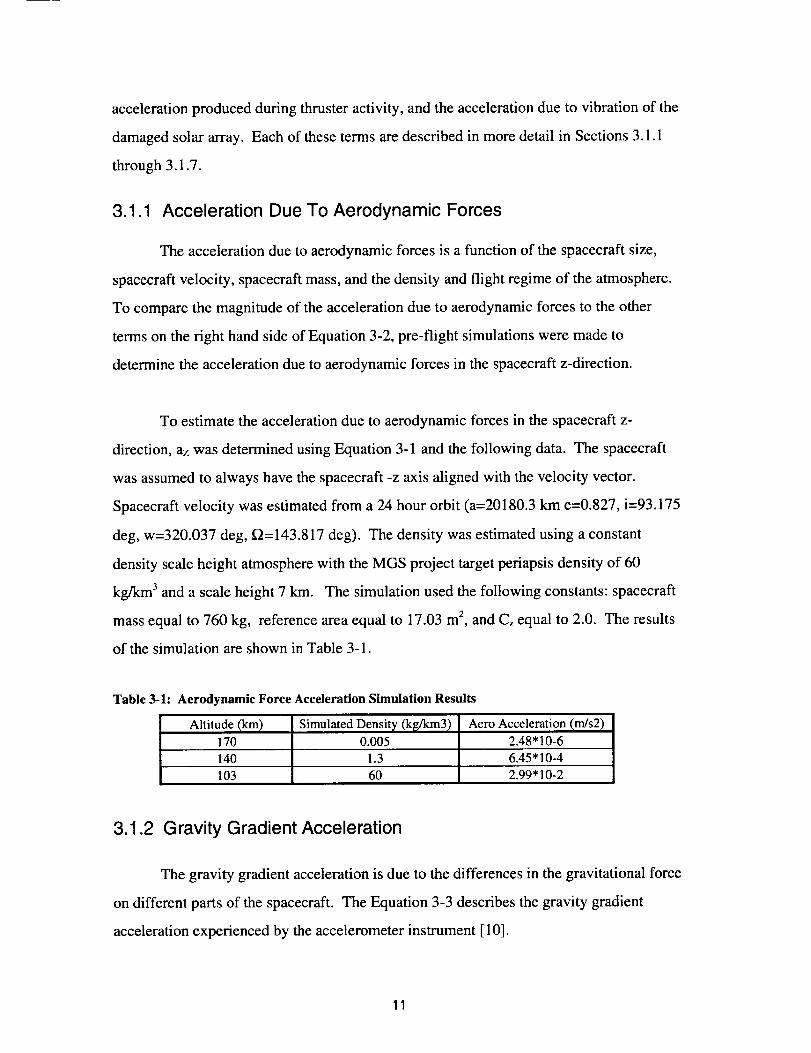
3.1.1 Acceleration Due To Aerodynamic Forces
The acceleration due to aerodynamic forces is a function of the spacecraft size,
spacecraft velocity, spacecraft mass, and the density and flight regime of the atmosphere.
To compare the magnitude of the acceleration due to aerodynamic forces to the other
terms on the right hand side of Equation 3-2, pre-flight simulations were made to
determine the acceleration due to aerodynamic forces in the spacecraft z-direction.
To estimate the acceleration due to aerodynamic forces in the spacecraft z-
direction, az was determined using Equation 3-1 and the following data. The spacecraft
was assumed to always have the spacecraft -z axis aligned with the velocity vector.
Spacecraft velocity was estimated from a 24 hour orbit (a=20180.3 km e=0.827, i=93.175
deg, w=320.037 deg, f2=143.817 deg). The density was estimated using a constant
density scale height atmosphere with the MGS project target periapsis density of 60
kg/km 3 and a scale height 7 km. The simulation used the following constants: spacecraft
mass equal to 760 kg, reference area equal to 17.03 m 2, and Cz equal to 2.0. The results
of the simulation are shown in Table 3-1.
Table 3-1: Aerodynamic Force Acceleration Simulation Results
Altitude (km) Simulated Densit)_ (k_krn3) Aero Acceleration (m/s2)170 0.005 2.48" 10-6
140 1.3 6.45"10-4103 60 2.99* 10-2
3.1.2 Gravity Gradient Acceleration
The gravity gradient acceleration is due to the differences in the gravitational force
on different parts of the spacecraft. The Equation 3-3 describes the gravity gradient
acceleration experienced by the accelerometer instrument [10].
11
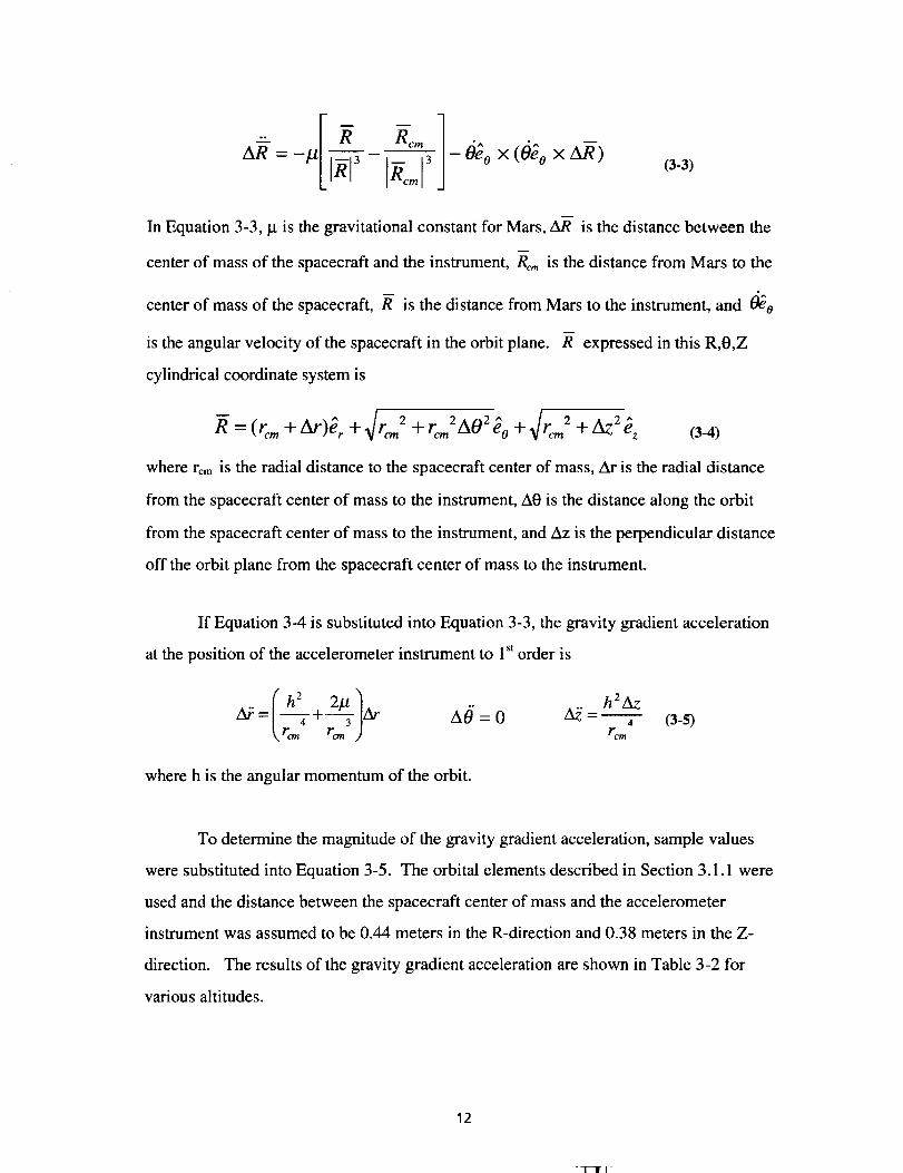
In Equation 3-3, _t is the gravitational constant for Mars, AR is the distance between the
center of mass of the spacecraft and the instrument, Re,, is the distance from Mars to the
-- "^
center of mass of the spacecraft, R is the distance from Mars to the instrument, and 0_0
is the angular velocity of the spacecraft in the orbit plane. R expressed in this R,0,Z
cylindrical coordinate system is
-_ = (rcm + Ar)_r + _/rcm 2 + rcm22,,A0 eo + x/rcm2 +Aze 2 ,, (3-4)
where rcm is the radial distance to the spacecraft center of mass, At" is the radial distance
from the spacecraft center of mass to the instrument, A0 is the distance along the orbit
from the spacecraft center of mass to the instrument, and Az is the perpendicular distance
off the orbit plane from the spacecraft center of mass to the instrument.
If Equation 3-4 is substituted into Equation 3-3, the gravity gradient acceleration
at the position of the accelerometer instrument to 1st order is
h2AzA0" = 0 ZkZ- 4 (3-bO
rc_
where h is the angular momentum of the orbit.
To determine the magnitude of the gravity gradient acceleration, sample values
were substituted into Equation 3-5. The orbital elements described in Section 3.1.1 were
used and the distance between the spacecraft center of mass and the accelerometer
instrument was assumed to be 0.44 meters in the R-direction and 0.38 meters in the Z-
direction. The results of the gravity gradient acceleration are shown in Table 3-2 for
various altitudes.
12

Table 3-2: Gravity Gradient Acceleration Simulation Results
Altitude
(km)170
140
103
Gravity Gradient Acc (m/s2)R 0 Z
1.60* 10 .6 0 6.54* 10 .7
1.65* 10 .4 0 6.76* 10 .7
1.69" 10 -6 0 6.98* 10 .7
If the spacecraft is always oriented with the spacecraft z-axis on the velocity vector (the 0
direction in the cylindrical coordinate system), the simulation results in Table 3-2
demonstrate the gravity gradient will have no first order effect on the acceleration
measured in the z-direction.
The spacecraft z-axis will not always remain aligned with the velocity vector,
therefore, other orientations of the spacecraft must be considered to determine the
maximum gravity gradient. The control system used for MGS limits the spacecraft to a 20
degree deviation of heading from the velocity vector during the aerobraking pass.
Assuming the spacecraft is 20 degrees off the velocity vector towards the radial direction
from the planet, the maximum gravity gradient acceleration measured by the spacecraft z-
axis accelerometer is 5.5* 10 .7 m/s 2. As shown in Table 3-1, the maximum gravity gradient
is less than 1 percent of the aerodynamic acceleration below 140 km. However, the
gravity gradient component is approximately 22 percent of the 170 km acceleration
estimate.
Since the main focus of this investigation was to estimate and predict density
values up to 30 km above the periapsis altitude, the gravity gradient was considered
negligible. If higher altitudes are examined with the methods outlined in this paper, the
gravity gradient term should be included in the development of the measured acceleration.
The gravity gradient term can be included by using Equation 3-5 to find the gravity
gradient acceleration in the R, 0, Z coordinate system and then transforming this
acceleration into the spacecraft coordinates by determining the orientation of the
spacecraft relative to the velocity vector.
13

3.1.3 Acceleration Due To Solar Pressure
The acceleration due to solar pressure is caused by solar radiation interacting with
the surface of the satellite. The solar pressure is a function of the size of the spacecraft,
the distance from the spacecraft to the sun and the orientation and reflecting properties of
the spacecraft surface. Equation 3-6 was used to examine the magnitude of the
acceleration due to solar pressure [11].
-asolarl= Fs A(l"k-qr)C°SOi (3-6)mc
In Equation 3-6, Fs is solar constant, 590 W/m 2 at Mars, c is the speed of light, A is the
cross-sectional area of the satellite in the direction of incoming radiation, m is the satellite
mass, qr, is the reflectance factor which ranges from 0 to 1 (0 corresponds to photon
absorption, i.e. no reflection, and 1 is perfect reflection) and 0i is the incidence angle of the
incoming radiation. To estimate the magnitude of the acceleration due to solar pressure,
the properties for spacecraft mass and area from Section 3.1. l, a reflectance factor of 1,
and an incidence angle of 0 degrees were substituted into Equation 3-6. Using these
values, the acceleration due to solar pressure was determined to be 8.8"10 .8 m/s 2 . When
compared to the calculations of acceleration due to aerodynamic forces, the value for
acceleration due to solar pressure was negligible and, therefore, omitted from the
calculation of measured acceleration.
3.1.4 Bias Acceleration
As stated in Section 2.1, the accelerometer instrument measures the voltage
necessary to keep a proof mass suspended inside a magnetic ring. The voltage reading
necessary to keep the mass in balance during periods of no acceleration is known as the
instrument bias. The acceleration reading corresponding to this instrument bias is the bias
acceleration. The bias acceleration is a function of instrument properties and instrument
14
"VII I

temperature. To determine the acceleration bias, the instrument must be continually
checked and the surrounding temperature continuously monitored such that drift, i.e.
change in the bias value as a function of time, can be determined.
For the MGS mission, bias was determined by monitoring the accelerometer
instrument during periods before and after entering the atmosphere. The bias acceleration
was then estimated over the entire pass by averaging the data from the pre- and post-
atmospheric entry periods. The pre- and post-atmospheric periods were defined by
instrument on and off times and an altitude limit of the atmosphere. For the MGS mission,
the altitude limit was set by examining the acceleration profile and selecting an altitude
well above the first indications of accelerations due to the atmosphere, typically 200 km.
3.1.5 Angular Motion Acceleration
The acceleration from the angular motion of the spacecraft is caused by the
accelerometer instrument not being at the center of mass of the spacecraft. This
acceleration can be estimated by the Equation 3-7 [12].
aa,,8.1,,r = _- X (_" X 7) + if- X ? (3-7)
The angular acceleration component is a function of the distance between the center of
mass of the spacecraft and the instrument, r, the angular rate of the spacecraft, co , and
the angular acceleration of the spacecraft, a .
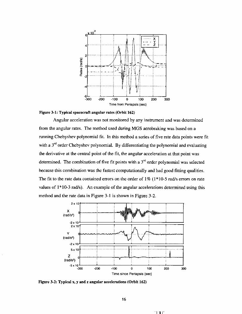
For the MGS mission, angular rate was determined by on-board gyros and shown
for a typical pass in Figure 3-1.
15
-3<10
J m i
' ...........i...........Vi,,.........
! !ji_ , i
: :,.4 ii,_ i !
-' 7: i 1
-6 i i i-300 -200 -100 0
J i
!'-........."x
....i: m+i.....]
i I
1 O0 200 300
Time from Periapsis (see)
Figure 3-1: Typical spacecraft angular rates (Orbit 162)
Angular acceleration was not monitored by any instrument and was determined
from the angular rates. The method used during MGS aerobraking was based on a
running Chebyshev polynomial fit. In this method a series of five rate data points were fit
with a 3 rd order Chebyshev polynomial. By differentiating the polynomial and evaluating
the derivative at the central point of the fit, the angular acceleration at that point was
determined. The combination of five fit points with a 3 rd order polynomial was selected
because this combination was the fastest computationally and had good fitting qualities.
The fit to the rate data contained errors on the order of 1% (1 "10-5 rad/s errors on rate
values of 1 * 10-3 rad/s). An example of the angular accelerations determined using this
method and the rate data in Figure 3-1 is shown in Figure 3-2.
X 2 x 100_
2x o'I i !
y ! ! .... _ ...... :
(rad/s2) _
-2x 10 J i
,x,of.................................,......'-ti ...............................................SxlO- :' :, i
-300 -200 -100 0 100 200 300
Time since Periapsis (see)
Figure 3-2: Typical x, y and z angular accelerations (Orbit 162)
16
111-

By examining the angular acceleration data in Figure 3-2, several spacecraft
activities can be observed. First, the spikes shown in the z-angular accelerations indicate
times of control system thruster activity. Second, the vibration of the SAM can be
observed by examining the x-angular accelerations.
The motion of the SAM, does cause the center of mass of the entire spacecraft to
move in the body. The term compensating for this motion, i.e. the term describing the
changing distance between the center of mass and the instrument, is neglected in Equation
3-7. This distance between the instrument and the center of mass was assumed constant
in this investigation because the spacecraft center of mass moves very litre due to panel
motion. One degree of panel motion only causes approximately 0.1 cm of center of mass
motion.
The magnitude of the acceleration due to angular motion was estimated using
Equation 3-7, the distance between the accelerometer instrument and the spacecraft center
of mass from Section 3.1.2, and the angular rate and angular acceleration in Figures 3-1
and 3-2. The maximum acceleration due to angular motion for this sample pass was
approximately 0.0008 rn/s 2. When this estimation is compared to aerodynamic force
acceleration estimations, the accelerations due to angular motion cannot be considered a
negligible contributor to the measured acceleration equation.
3.1.6 Thruster Acceleration
The exact spacecraft reactions to thruster activity are very difficult to determine
because the force of the thruster is a combination of several quantities that are difficult to
model [13], such as, the effectiveness of the blow down phase, the temperature of the
catalyst, and the interference of the thruster plume with the atmospheric flow [6].
The MGS spacecraft has 12 attitude control thrusters located in four pods off the
lower corners of the spacecraft bus (Figure 2-1). In each pod, two nozzles point in the
spacecraft negative -z direction and one in the roll direction (rotation about z). For the
17
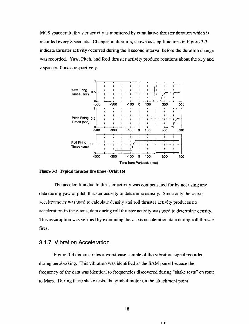
MGSspacecraft,thrusteractivity is monitoredby cumulativethrusterdurationwhich is
recordedevery8 seconds.Changesin duration,shownasstepfunctionsin Figure3-3,
indicatethrusteractivityoccurredduringthe8 secondintervalbeforethedurationchange
wasrecorded.Yaw,Pitch,andRoll thrusteractivityproducerotationsaboutthex, y and
z spacecraftaxesrespectively.
Yaw FiringTimes (sac)
Roll FiringTimes (sac)
I ,: i i i i i+............!.............+---
: : : f!
-500 -300 -100 0 100 300 5001
Times(sac)PitchFiring O.t ..... }+...... _+_i..... i ..... i_+ i_____i..... i ..... i ...... i ..... i...
-500 -300 -100 0 100 300 500
-500 -300 -100 0 100 300 500
Time from Periapsis (sec)
Figure 3-3: Typical thruster fire times (Orbit 16)
The acceleration due to thruster activity was compensated for by not using any
data during yaw or pitch thruster activity to determine density. Since only the z-axis
accelerometer was used to calculate density and roll thruster activity produces no
acceleration in the z-axis, data during roll thruster activity was used to determine density.
This assumption was verified by examining the z-axis acceleration data during roll thruster
fires.
3.1.7 Vibration Acceleration
Figure 3-4 demonstrates a worst-case sample of the vibration signal recorded
during aerobraking. This vibration was identified as the SAM panel because the
frequency of the data was identical to frequencies discovered during "shake tests" en route
to Mars. During these shake tests, the gimbal motor on the attachment point
18
-q-I I

between the bus and the SAM panel was activated in quick bursts to try to vibrate the
panel.
O
C
O
35
3O
25
20
15
I0
5
0
-5-200
| i ! |
= ; , ,
-150 -100 -50 0
i .,- ....... , .....
50 100 150
Time Since Periapsis 95 (sec)
200
Figure 3-4: Acceleration data with large amplitude vibrations (Orbit 95)
Assuming that the SAM panel was vibrating during the pass, a model was created to
estimate the effect of this vibration on the measured acceleration.
In the model, the SAM and the remaining parts of the spacecraft, the bus and the
solar array on the +y spacecraft axis (BUS+SAP), were assumed to be two separate
bodies. Aerodynamic forces on the two bodies were neglected to isolate the acceleration
contribution of the panel vibration measured by the z-axis accelerometer. The two bodies
were attached by a spring at the suspected SAM yoke crack line, as shown in Figure 3-5.
o,e" " " L
. : - - ..... >y
0 XM_ 2
V
Z2
, 0 ! ,'
I' B_S+SAP
a _. _ C_nter of Mass
L _
v (X into Paper)Z
Figure 3-5: Diagram of 2-body 4 DOF model used to estimate moving panel acceleration
19

The spring is described by Equation 3-8, developed in shake tests during cruise [Personal
Communication, W. Willcockson, 8/22/97]. In this equation, the spring torque, T, is a
function of the deflection angle, 0_.
T = (1300 in- lbs) ,O L3deg (3-8)
To construct the model, rotations about the spacecraft y and z axis and translations
in the x-direction were neglected. The kinetic and potential energy of the two body, 6
degree of freedom (DOF) system was calculated and are shown in Equation 3-9.
1 2 1 "2 1T_ysw.=-_m,(:Y, + Z,2) +'_ IxX.Us+SAprO, +_rth()22+Z.22)
1
+5Ixxsau(SaMcom,(_O,2-2S_SOa +_0, 2)
(3-9)
1
V.y,,_., = [. MdO = f (Tc Ox" )dO - X. + 1 TcO_x.+,
The z2 and y2 coordinates can be expressed in terms of the remaining coordinates using
Equation 3-10, reducing the system to 4 DOF.
Y2 = Yl- acos0_ -bsin0_ - Lcos(02 -0_) (3-10)
z2 = zt- a sin01 + bcos01 + Lsin(02 -Ol)
When Equation 3-10 is substituted into Equation 3-9 and the Lagragian is formed, the z_,
y_, 0_ coordinates were found to be cyclic. Using conservation of the conjugate
momentum in z_, y_ and 0_, and assuming no exterior forces and small angle
approximations, the equations of motion for this system were developed and are shown in
Equation 3-1 1.
(_ + m2)j; _ + (-m2b- nhLsin00)S/) I + (m2Lsin00)S/) _ = 0
(ma + m2)_ , + (-rn2a - nhLcos00)S _ + (m2Lcos00)&) } = 0 (3-11)
_1(-m2a - m2Lcos 0o) + )l (-rn2b - nhLsin 00)
+ t5[9_(-nhaL cos 0o- m2L2 - nhbL sin 00 - IxxsAu(s_u,,,,m))
+/_(m2 a2 + 2m2aLcosOo + rn2L2 + tn2b2 + 2nhbL sin Oo + Ix.xBvs+_e + lxxsau(sau, om)) = 0
20
"'vIr V
In this problem 01 is the angular acceleration in the spacecraft x-direction, which was
determined from onboard gyro data as shown in Section 3.1.5. Equation 3-1 ! is solved for
zl, the acceleration of the BUS+SAP center of mass due to the motion of the SAM panel. A
complete derivation of the system is shown in Appendix B.
An important note is that by assuming the BUS+SAP and SAM are separate
masses, the gyros located on the BUS are only monitoring the BUS+SAP body.
Therefore, to identify the acceleration from spacecraft angular motion described in Section
3.1.5, the center of mass of the BUS+SAP body must be used instead of the entire
spacecraft center of mass to determine the distance, r, in the angular motion equation,
Equation 3-7. This distance, r, is assumed constant because the BUS+SAP body is
considered rigid.
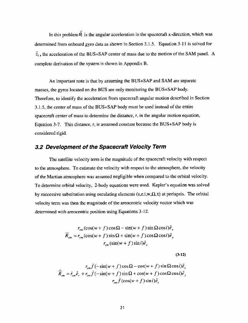
3.2 Development of the Spacecraft Velocity Term
The satellite velocity term is the magnitude of the spacecraft velocity with respect
to the atmosphere. To estimate the velocity with respect to the atmosphere, the velocity
of the Martian atmosphere was assumed negligible when compared to the orbital velocity.
To determine orbital velocity, 2-body equations were used. Kepler's equation was solved
by successive substitution using osculating elements (a,e,i,w,_,x) at periapsis. The orbital
velocity term was then the magnitude of the areocentric velocity vector which was
determined with areocentric position using Equations 3-12.
re,, (cos(w + f) cosf2 - sin(w + f) sin_cosi)_ x-- , ^
Rcm = rcm (cos(w + f) sin _ + sin(w + f) cos_ COSl)ey
rcm (sin(w + f) sin i)_
(3-12)
re,. f (- sin(w + f) cosf2 - cos(w + f) sin f2 cosi)_x
R--'_ = ro, er + rc,,J_(- sin( w + f) sinf_ + cos(w + f)cos_cosi)_y
ro, jk (cos(w + f) sin i)_
21

In Equation3-12,rcmis theradialposition,w is theargumentof periapsis,f is thetrue
anomaly,£2 is the longitude of the ascending node, and i is the inclination.
Since periapsis osculating elements only represent the orbit at periapsis, using 2-
body equations away from periapsis resulted in errors in position and velocity. To
estimate these errors, areocentric position was used as a measure of the effectiveness of
the 2-body equation procedure. A simulation was developed which determined the error
between a known orbit and an orbit generated from the 2-body equation using periapsis
osculating elements [Personal Communication, C. Acton, 9/6/97]. First, the exact position
and velocity for several times near periapsis of a sample orbit were generated. Next, a set
of osculating elements were generated at periapsis for the same orbit. Finally, the position
developed from these osculating elements was compared to the exact position and the
error in range was calculated. The results of the study for pre-mission sample orbit #34
["MGS Orbit Propagation and Timing Geometry File v001:optg_i_970912-
980219_ab0422bl", JPL May 8, 1997. Available from MGS NAV Team] are shown in
Table 3-3.
Table 3-3: Results of Range Error Study Between Exact Ephemeris and Ephemeris Generated FromOsculating Elements at Periapsis
Time From Periapsis
(sec_
240
Approx. Areodetic
Altitude (km)186.2
Range Error
[Exact-Ke_ler I (km_0.218
200 167.2 0.175
150 136.4 0.130100 118.4 0.081
50 107.5 0.027103.90 0.000
In Section 5, the range error is converted to equivalent density error so that a comparison
to other process errors can be made.
3.3 Development of the Ballistic Coefficient Term
The ballistic coefficient is composed of the force coefficient, the spacecraft
reference area and the mass of the spacecraft. The spacecraft mass was assumed constant
22
duringanaerobrakingpassbecausefuelusageby controlsystemthrusterswassmall
(<< lkg) comparedto thetotalspacecraftmass(approx.760kg). Thespacecraft
referenceareawascalculatedasthecross-sectionalareaseenby theflow whenthe
spacecraftis in theaerobrakingconfigurationwith thespacecraft-z axisalignedwith the
velocityvector. Theforcecoefficientwasdeterminedby developinganaerodynamic
databaseof forcecoefficientsandinterpolatingthevalueof thecoefficientby knowingthe
spacecraftorientation,andby estimatingthepaneldeflectionangleandthedensityof the
atmosphere.Thefollowing sectionsdescribethedevelopmentof theaerodynamic
databaseandtheuseof thedatabaseto determineforcecoefficients.
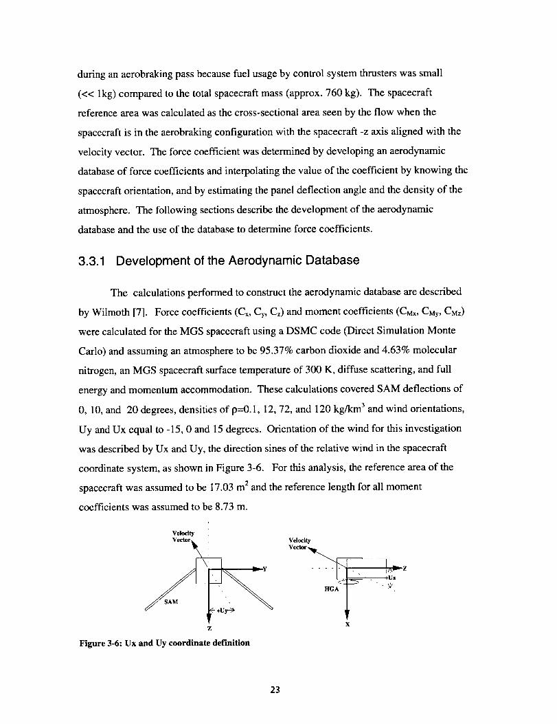
3.3.1 Development of the Aerodynamic Database
The calculations performed to construct the aerodynamic database are described
by Wilmoth [7]. Force coefficients (Cx, Cy, Cz) and moment coefficients (Cux, CMy, CMz)
were calculated for the MGS spacecraft using a DSMC code (Direct Simulation Monte
Carlo) and assuming an atmosphere to be 95.37% carbon dioxide and 4.63% molecular
nitrogen, an MGS spacecraft surface temperature of 300 K, diffuse scattering, and full
energy and momentum accommodation. These calculations covered SAM deflections of
0, 10, and 20 degrees, densities of p=0.1, 12, 72, and 120 kg/km 3 and wind orientations,
Uy and Ux equal to -15, 0 and 15 degrees. Orientation of the wind for this investigation
was described by Ux and Uy, the direction sines of the relative wind in the spacecraft
coordinate system, as shown in Figure 3-6. For this analysis, the reference area of the
spacecraft was assumed to be 17.03 m 2 and the reference length for all moment
coefficients was assumed to be 8.73 m.
Vdoctty
VelocityVector
. 4Ux
_ +Uy-->
XZ
Figure 3-6: Ux and Uy coordinate definition
23

Figures 3-7 and 3-8 summarize the results from the aerodynamic database
generated for aerobraking operations. Figure 3-7 demonstrates how the force coefficient
varies with density and panel deflection. Note any density value below 0.1 kg/km 3 was
considered free molecular flow (corresponding to Knudsen numbers greater than 1).
o"
i$
O
O
OII
2.3
2.2
2.1
2
1._J
1.8
1.7
1.6
1.5
i iiiiiii i i iiiiii -_-= No SAM Delfection iii
'"::"!'!'!!!!! .... i"i'ii'i!!i ....... 10deg SAM deflection ::::::
i i:: :::::::::: i :: i::i::ii -o-- 20deq SAM deflection ii::
....
.... i.,i-i,iiiii, i..i..!!.!!!!...."-:::!_!_iii!!....!..!.!-:-!_.....!..!-!!.!!!!:
." ; : 2;;;: ; ; ;:12;: ......................
....i iiiiiii....i?iiiiii....!!i!i!i! ....if+!!! ,i?ii?ili: : ::::': : : :;:;:: : : : ::::: : " ";': ........
0 1 10 0 101 10 2 10 3
Density (kg/km 3)
Figure 3-7: Force coefficient in spacecraft z-direction, C=, vs. density level for all panel deflections
Each 10 degrees of panel deflection reduces Cz by approximately 5 percent, due primarily
to reduction in frontal area [6]. Note that change in Cz is linear with change in panel
deflection.
Figure 3-8, demonstrates how the Cz force coefficient varies with wind orientation.
The left side of the figure shows the contour generated with no-deflection and a density of
12 kg/km 3. The fight side of Figure 3-8, demonstrates the contour generated with a
density of 12 kg/km 3 and 10 degrees of SAM panel deflection.
24
I|1-

0.25
0.1
_'0
-0.1
0 Degrees Deflection
-025 ..... ....,........ .............025-0.25 -0.1 0 0.1 0.25 -0.25
0.25
0.1
_'0'-I
-0.1
10 Degrees Deflection
-0.1 0 0.1 0.25
Ux Ux
Figure 3-8: Cz tables for free molecular densities (0 degree SAM Deflection and 10 degree SAMDeflection)
With zero panel deflection, Cz is nearly symmetric about Uy and offset approximately 2
degrees from Ux equal to zero. This is due to the geometric symmetry about the
spacecraft z-x plane and the asymmetry caused by the high gain antenna about the z-y
plane. With 10 degrees panel deflection, the peak Cz value decreases and shifts
approximately 2.8 degrees toward positive Uy. This decrease is due to area change from
panel deflection. The shift demonstrates that during 10 degree panel deflections, the
largest area occurs when the spacecraft is rotated 2.8 degrees about the spacecraft
negative x-axis.
Important to the analysis of spacecraft dynamics were DSMC simulations done on
the SAM disregarding the rest of the spacecraft. Using the same assumptions mentioned
previously, analyses were made to calculate force and moment coefficients of the panel for
all wind orientations, all deflection angles and all density ranges used in the analysis of the
entire spacecraft. The entire database of force and moment coefficient values used during
MGS aerobraking for the entire spacecraft and the SAM panel without the remaining parts
of the spacecraft is shown in Appendix C.
25

3.3.2 Determining Force Coefficients
Force coefficients were determined by interpolation of the aerodynamic database.
Inputs to this interpolation were the orientation of the relative wind, density, and panel
position. Density and panel position were determined by the iterative scheme discussed in
Section 4.4.3. The orientation of the incoming wind was determined by combining the
orbital velocity and the atmospheric winds in the spacecraft centered system.
To determine the orbital velocity in the spacecraft system, quaternions produced
onboard the spacecraft, shown in Figure 3-9, were used to form a direction cosine matrix,
(DCM) using Equation 3-13 [14]. Using the DCM, the orbital velocity in the planet
centered system (Section 3.2) can be transformed into the spacecraft centered system.
t-O
O
0.4
0.2
0
-0.2
-0.4
-0.6
-0.8
-1-300
- i i
.......... ;.......... i.......... i ......... i ......... : ..........
........ .; .......... ; .................... _ ......... ,;.........
q4i :•-- - ..........:---.-.... _........ i......... _.........
, i i _ i
-200 -100 0 100 200 300Time from Penapsis (sec)
Figure 3-9: Typical quaternions (Orbit 162)
Iqt --q2 2 -- q3 2 + q4 2 2(q_q2 + q3q4)
[DCM] = I 2(q_qz -q3q4) --q] 2 +q2 2 --q3 2 +q4 2
2(q_q3 +qEq4) 2(q2q3 -q_q4)
2(qlq3 - q2q4)
2(q2q3 + qlq4)
_q]2_q22 +q32 +q42
26
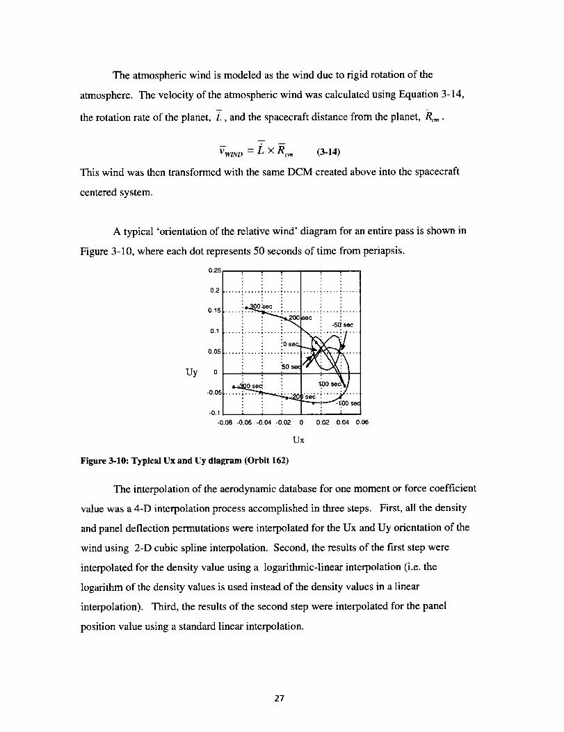
The atmosphericwindis modeledasthewind dueto rigid rotationof the
atmosphere.Thevelocityof theatmosphericwind wascalculatedusingEquation3-14,
therotationrateof theplanet, L, and the spacecraft distance from the planet, R-c,, •
-T" --
v--wino = L × Rcm (3-14)
This wind was then transformed with the same DCM created above into the spacecraft
centered system.
A typical 'orientation of the relative wind' diagram for an entire pass is shown in
Figure 3-10, where each dot represents 50 seconds of time from periapsis.
0.25., ., ! , ;
0.2 ...... • ..... ; ................. ; ..... • .....
Uy
0.15
0.1
0.05
0
-0.05
-0.1
-0.08 -0.06 -0.04 -0.02
......_.i ..........._....._.....i ..-_osec i !: : : _ : -5{1 sec
......_!....._....._oso___.....':....i i _os_ • "!"--'_i I: : : r_-_)_: ,_oos_W
....... . ..... :_ _e_"."'5:g ...._-1:00 se(
; ; ; : ;
0.02 0.04 0.06
Ux
Figure 3-10: Typical Ux and Uy diagram (Orbit 162)
The interpolation of the aerodynamic database for one moment or force coefficient
value was a 4-D interpolation process accomplished in three steps. First, all the density
and panel deflection permutations were interpolated for the Ux and Uy orientation of the
wind using 2-D cubic spline interpolation. Second, the results of the first step were
interpolated for the density value using a logarithmic-linear interpolation (i.e. the
logarithm of the density values is used instead of the density values in a linear
interpolation). Third, the results of the second step were interpolated for the panel
position value using a standard linear interpolation.
27

4. Operational Data Reduction Procedure
Section 4 will discuss the procedures and studies performed to create the
operational data reduction procedure used to determine densities from accelerometer data
during the 1st phase of aerobraking at Mars. First the operational scenario including
mission constraints and the operational accelerometer instrument is discussed. The
amount of accelerometer data necessary to perform the operational responsibilities is
determined. Next, the data reduction procedure is described using Section 3 methods
modified for the MGS operational scenario. Finally, several extra products of the data
reduction procedure as well as prediction methods are discussed.
4.10perationalConstramts
To be effective during aerobraking operations, methods used to calculate density
have to be computed quickly and accurately over a range of altitudes. According to MGS
project constraints, all accelerometer data analysis must be completed within 2 hours of
receiving data. Since most of this time should be devoted to the analysis of density trends,
the procedure to calculate density for the entire orbit should be completed in one quarter
of the allowable time or 30 minutes. To fully understand the atmosphere, the calculation
of density must be accurate over a large range of altitudes. The methods were designed to
be accurate over an altitude range of 30 km above periapsis. This altitude range was
chosen to allow density to be calculated over approximately 4 scale heights.
The data provided to perform the accelerometer data reduction process included
all values shown in Table 4-1. These data types were provided every aerobraking pass by
telemetry. Note accelerometer data rate for the first 15 aerobraking orbits was 10 samples
every 8 seconds. This data rate was increased to 1 sample every 0.1 seconds when
aerobraking resumed after the investigation of the panel over-extension.
28
-'1 |1
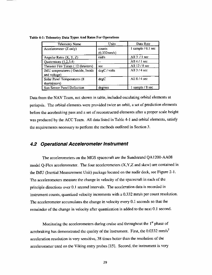
Table 4-1: Telemetry Data Types And Rates For Operations
Telemetr_ NameAccelerometer (Z only)
Angular Rates (X, Y, Z)
Quaternions (1,2,3,4)Thruster Fire Times ( 12 thrusters)IMU temperatures ( Outside, Inside
and voltage)Solar Panel Temperatures (8
thermistors)Sun Sensor Panel Deflection
Units
counts
(0.332ram/s)rad/s
sec
degC / volts
Data Rate
I sample / 0.1 sec
All 3 / 1 sec
All 4 / 1 secAll 12 / 8 sec
All 3 / 4 sec
degC All 8 / 4 sec
degrees 1 sample / 8 sec
Data from the NAV Team, not shown in table, included osculating orbital elements at
periapsis. The orbital elements were provided twice an orbit, a set of prediction elements
before the aerobraking pass and a set of reconstructed elements after a proper scale height
was produced by the ACC Team. All data listed in Table 4-I and orbital elements, satisfy
the requirements necessary to perform the methods outlined in Section 3.
4.2 Operational Accelerometer Instrument
The accelerometers on the MGS spacecraft are the Sundstrand QA 1200-AA08
model Q-Flex accelerometer. The four accelerometers (X,Y,Z and skew) are contained in
the IMU (Inertial Measurement Unit) package located on the nadir deck, see Figure 2-1.
The accelerometers measure the change in velocity of the spacecraft in each of the
principle directions over 0.1 second intervals. The acceleration data is recorded in
instrument counts, quantized velocity increments with a 0.332 mm/s per count resolution.
The accelerometer accumulates the change in velocity every 0.1 seconds so that the
remainder of the change in velocity after quantization is added to the next 0.1 second.
Monitoring the accelerometers during cruise and throughout the 1st phase of
aerobraking has demonstrated the quality of the instrument. First, the 0.0332 mm/s 2
acceleration resolution is very sensitive, 38 times better than the resolution of the
accelerometer used on the Viking entry probes [15]. Second, the instrument is very
29

stable.Duringthetravelto Mars,two separatemeasurementstakenbeforetrajectory
correction maneuvers (TCM), 8 months apart, resulted in a bias change of only 2%
(TCM-1 bias=5.62 +/- 0.12 counts/0.1 sec, TCM-2 bias=5.70 +/- 0.05 counts/0.1 sec).
During aerobraking, the bias remained at 5.66 +/- 0.005 counts/0.1 sec, varying only 0.1
percent over the entire 201 passes (192 days) of the 1stphase of aerobraking. This bias
stability is due to the temperature control of the instrument. The temperature of the IMU
box is monitored by two temperature sensors, one inside the box and one on the box
housing, and controlled by a single heater. A sample plot of the output of the two sensors
and the voltage to the heater is shown in Figure 4-1.
62.2l ,J_, ', '. : :
IMU Block _.!,...L._.,........ : : :
•e 0( e0O) i -i ........i i i i
61 3.300 -200 -100 0 100 200 300
27 : i i ; :
IMU Housing _tTemp (degC) 26.5
26 -300 -200 - 1O0 0 1O0 200 300
135[ .....• i i i i :
Voltage toHeater(volts) 13 ......... :......... " ........ !" . !
12.5.300 -200 -1 O0 0 1 O0 200 300
Time from Periapsls (sec)
Figure 4-1: Typical IMU temperatures and voltage to IMU heater (Orbit 162)
Examining Figure 4-1, the quantum of temperature measurement inside the IMU is 0.117
°C and the highest temperature variation was 2 quanta over a period of 4 seconds. To
calculate the effect of this temperature variation on accelerometer measurents, the
accelerometer manufacturer' s estimate of 0.3 counts of acceleration change per °C of
temperature change was used ["Sundstrand Data Control's Q-Rex Servo Accelerometers:
QA-1200 and QA-1300 Data Sheet.", 1984. Available from The Sundstrand Data
Control Corporation]. Therefore, a 2 quanta temperature variation over 4 seconds
resulted in an acceleration change of 5.8"10 -6 m/s 2. When compared to the acceleration
values of Section 3.1.1, the value of acceleration due to temperature change was negligible
for altitudes within 30 km of periapsis. By further examining Figure 4-1 above, the
3O
temperaturedid notexhibit anyincreaseordecreasethatwouldindicateatmospheric
heatingwasaffectingtheaccelerometersinsidetheIMU.
4.3 Quantity of Accelerometer Data Necessary to Perform
Operations
To determine the quantity of accelerometer data necessary to complete all
operational responsibilities, a simulation was developed to test the amount of
accelerometer data needed to reproduce a known atmospheric trend. The simulation
examined several different amounts of accelerometer data by first creating a atmosphere
with a known density trend, and then simulating the spacecraft with an accelerometer
instrument moving though that atmosphere. If the quantity of data being examined was
sufficient, the results from the model should reproduce the known atmosphere.
To set up the simulation the following parameters and assumptions were used. To
model the spacecraft motion, a 24 hour orbit (a=20! 80.3 e=0.827, i=93.175 deg,
w=320.037 deg, ff2=143.817 deg) was used. To model the accelerometer instrument,
Equation 3-1 was solved for the acceleration, az, and then this acceleration was quantized
and accumulated as described in Section 4.2. The coefficient of drag, spacecraft mass and
spacecraft cross-sectional area were all assumed to be constant (CD=2, mass=760 kg,
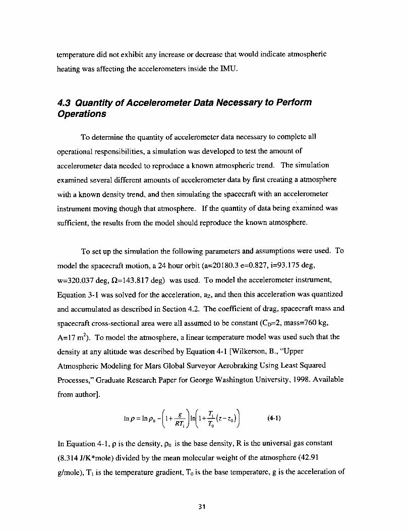
A=I7 m2). Tomodel the atmosphere, a linear temperature model was used such that the
density at any altitude was described by Equation 4-1 [Wilkerson, B., "Upper
Atmospheric Modeling for Mars Global Surveyor Aerobraking Using Least Squared
Processes," Graduate Research Paper for George Washington University, 1998. Available
from author].
In Equation 4-1, p is the density, po is the base density, R is the universal gas constant
(8.314 J/K'mole) divided by the mean molecular weight of the atmosphere (42.91
g/mole), TI is the temperature gradient, To is the base temperature, g is the acceleration of
31

gravityonMars(3.4755mJs2), z is the altitude, and Zo is the base altitude. For this
simulation, the following values were assumed: p0=60 kg/km 3 , T1 = 2.862 K/km,
T0=131.2 K, zo=103 km.
The simulation investigated three data rates including: one 0.1 second
measurement every second, ten 0.1 second measurements every 8 seconds, and ten 0.1
second measurements every second. For the second case, the 10 measurements were
contiguous and cover an entire second. The third case represented the "full potential data
rate", or a measurement every 0.1 seconds during the drag pass. All the data rates were
averaged with a 40 second running mean. The results are shown in the three plots in
Figure 4-2.
0,1 s_eJ sec Data
• 200 / ........ ; ........ ; ........
1'°I....'........i..............i...............180_ ............. !.............. - ..............
170: _._-. ....... :.,.............. !...............
350 .... 'm " m_m_ .............. : ...............
130........... ..............110 ............ _ ..... _....._:100
I sec/Ssec Data200. ; ....... : ........
,,°t' .........i..............i.............t_ot.............!..............}.............
g 1_o'?!;"i.'iiiii;;.'iii:i:iiiiiii;i;iiii;i;150
140
130
120
110
100
-2 -1 100 101 -2 -1 t0010 10 10 10
Log Acceleration (counts/0, Is) Log Acceleration (counts/0. ls)
lsec/sec Data200 ..........................
19o .............. i .............................
18o!.............. i ...........................
1701_
160
_1501
1401
1301
1201
1101
100 _-2 -1
10 10 10 100 10
Log Acceleration (counts/0. ls)
Figure 4-2: Results of Accelerometer Data Rate Simulation
In Figure 4-2, the line represents the a priori density model converted into acceleration
and the circles represent the output from the simulation.
A very important feature of this study was that a change in the start time of the
simulation produced different results. Since it is unknown when the start of the
atmosphere would occur relative to the measurements that were sampled, many different
density profiles were possible. Case 1 has 100 possible density profiles, case 2 has 80
possible density profiles, and case 3 has 10 possible density profiles. Each profile was
achieved by changing the start time of the simulation by 0.1 seconds. The results of the
three cases with all possible outcomes is shown in Figure 4-3.
32

200
190
180
170
=E" 160
._ 150140
130
120
110
10010-2
100 Permutations*- 0. lsec/sec case
..... t ....................... i ..............
...p.. q .................. i .............
_iii.,.._..............!..............
.....!.._.:.*..............:..............
161 lo0Log Acceleration (oounts/0. ls)
80 Permutation- lsecJSsec case200 ................. ,. .......
190 .l ......... ::.............. i .............
180 '"* ......... _............... i..............
,,o]...... ,.,!..............!..............
130
120
110
101 10010"2 ld 1 100 101
Log Acceleration (oounts/0.1 s)
10 Permutations-- I sec/sec case200, ........ . ................
1,ot..............!..............!..............
17ot_............ i .............. _.............160_1k_ ii--: .............. !..............
t............ .................
10010-2 I(_I 100 101
Log Acceleration (counts_. ls)
Figure 4-3: Results of accelerometer data rate simulation considering all possible outcomes
Using Figure 4-3, the effectiveness of each case was determined by considering the
errors of all possible outcomes from the known atmosphere. The error of each point was
calculated by subtracting the known acceleration from the model acceleration and then
dividing by the known acceleration. Since the effectiveness of the data rates varies with
altitude, several different altitude ranges were inspected: 110 - 120 km, 120 - 130 km,
130 - 140 km, 140-150 km, 150-160 km, and 160-170 kin. In each of these altitude
ranges, the standard deviation of all the errors in the altitude range were calculated and
shown in Table 4-2.
Table 4-2: Results From Reliability of Accelerometer Data Simulation
Altitude
Range (km)
110-120
120-130
130-140
140-150
150-160
160-170
Model Drag Accel
Range
(counts/0.1 sec)3.60 --) 1.00
1.00--)0.34
0.34 --) 0.13
0.13 -') 0.06
0.06--)0.03
0.03 --) 0.01
Case 1 StdDev (%)
(0.1 sec of data/sec)
5.12
14.60
28.60
44.63
76.21
98.03
Case 2 StdDev(%)
(1 sec of data/8sec)
Case 3 StdDev(%)
(1 sec of data/sec)
4.03
i.57 0.89
0.44
13.56
36.22
49.97
70.13
0.79
1.85
4.37
6.84
If the standard deviation limit of an accurate analysis is set at 5%, Table 4-1 shows
that case 1 can only be used over the 17 km range between periapsis at 103 km and 120
km. This corresponds to acceleration values greater than 1.0 counts/0.1sec. Case 2
extends this range to 130 km corresponding to acceleration values greater than 0.34
counts/0.1 sec. Case 3 can be used up to 160 km or acceleration values greater than 0.03
33

counts/0.1 sec. Since case 2 and case 3 were accurate over an altitude range of 30 km
above periapsis, both were used during MGS operations.
4.4 Operational Data Reduction Process
The accelerometer operational data reduction process was designed to determine
density during the entire aerobraking pass by using inputs from the MGS spacecraft and
the MGS NAV Team. The process is broken down into 4 steps: calculate orbital
parameters, remove non-aero accelerations, the iterative density process and data
averaging. The diagram showing the relationships of these steps is given in Figure 4-4.
__ Orbital _j Calculat e
NAV Orbital Air, Lat, Long, LST, SZA
Team /Elements _J Parameters
[-Quaternions I !
I t J Pos, Vel Vel, Ux, Uy /
//Telemetry Rates, C Remove / ,,era,,vei I-- _
/ _,"_,_;rq I Non-hero -aaeroq_ Density |Densityt_ _ Uata. _---
Figure 4-4: Data reduction processflow chart
/ Averaged /
Density vs.
Orbital /Propedies /
I
As stated in Section 4.1, to function effectively in aerobraking operations, the data
reduction procedure was originally allocated 30 minutes to complete. The average time
from initial input of data to a final output of density was approximately 7 minutes. This
time was for 16 minutes of data (approximately 9600 acceleration points) using a 200
MHz Pentium processor with 32 MB of memory.
4.4.1 Calculate Orbital Parameters
To develop atmospheric trends, density measurements were compared to various
orbital parameters such as areodetic latitude, areodetic altitude, longitude, local solar time
(LST) and solar zenith angle (SZA). These parameters were determined from the
areocentfic position vector and velocity vector, Mars planetary physical data shown in
Appendix D, the position of the Sun in the Mars centered system, and the following
formulas in Equation 4-2.
34
":]-| ]

tan 0 L'
tan O_ = (! _ f,j
aO-
= ]l-f. 2-f )cos O '
SZA = cos -_ (sin 6s_ * sin Ssc
+ cos t_svN * cOSfsc *cos(asc - Otsc))
), 24LST = ( sc T
Equation 4-2: Equations for calculating orbital parameters
In Equation 4-2, rcm is the radial distance of the spacecraft, z is areodetic altitude, a is the
planet equatorial radius, fm is the planet flattening, 0L is the areocentric latitude, 0L' is the
areodetic latitude, txs_ is the right ascension of the sun in the Mars equatorial system, t_
is the right ascension of the spacecraft in the Mars equatorial system, _Ss_ is the declination
of the sun in the Mars equatorial system, _5_ is the declination of the spacecraft in the Mars
equatorial system and /.. is the rotation rate of Mars. Areocentric latitude was calculated
by Napier's Rule using argument of periapsis, true anomaly, and inclination.
The 'calculate orbital parameters' process also determined the orientation of the
wind for the entire pass. The procedure described in Section 3.3.2 was used to calculate
the Ux and Uy parameters given the areocentfic position vectors and areocentric velocity
vectors, and the quaternions from the spacecraft telemetry.
4.4.2 Remove Non-Aero Accelerations
The 'remove non-aero accelerations' process was divided into three steps. First,
the acceleration due to angular motion and SAM vibration were determined using the
procedures described in Section 3.1.5 and Section 3.1.7 and removed from the measured
acceleration. The vibration acceleration procedure was not used during the 1st phase of
aerobraking due to the late development of this procedure, but is mentioned here to show
its correct position in the overall data reduction process. Second, the thruster acceleration
35

procedurewasappliedaccordingto Section3.1.6,byremovingall accelerometerdata
insidethe8 secondintervalduringyawandpitch thrusteractivity. Third, thebias
accelerationwascalculatedasdescribedin Section3.1.4.
Dueto thestabilityof the instrumentandtheunchangingtemperatureconditions
of theIMU, thebiasdrift equationdevelopedto describeatime varyingbiasoverthe
entireaerobrakingpasswasreducedtojust aconstantterm. Thebiasaccelerationis then
removedfrom themeasuredaccelerationleavingtheestimatefor theaccelerationdueto
aerodynamicforces.A typicalplot of thebiascalculationis showninFigure4-5.
Q)
r-.._
o
0
57._ !
T
57 -_
56.E ........ : ....
56.E ........ _....
56 A ........ _....
56._ ........ _....
56 ._
55._
-400 -300
i : i i
:o_nst Bi_s---56. "4_.4_ou_s/! se_ .......
:,gb._..__ ..In_i.d¢.... i __ .....................Atmosphere:
• ! ! i i ! !
-200 -100 0 100 200 300 400 500
Time from Periapsis (sec)
Figure 4-5: Typical accelerometer instrument bias calculation
4.4.3 Iterative Density Process
Density was determined through a double-loop iterative process which estimates
force coefficient and panel position to calculate density. A diagram of the process is
shown in Figure 4-6.
36
T| V

/ Determine
Acc _ Density AssumingData / "lCd=2"0 and Panel
/ I Deflection=O
/vO,=/T!ASDSe_lm_ioPan;I-I
No
Yes_
Determine Z and Y Forceand X Monent Coeficients
For Panel
_ Determine
Density
Figure 4-6: Development of density flow chart
Wind /Coordinates/
(ux,uy) /
H DeterminePanel Position
N_Yes--_
Determine Z-Force
Coeficient For Spacecraft
As shown in Figure 4-6, aerodynamic acceleration was used to calculate the first density
estimate assuming no deflection of the SAM panel and a force coefficient of 2.0. Next
Ux and Uy data, the density, and panel deflection equal to zero were used to interpolate
force and moment coefficients at every point during the pass for the SAM panel using
methods outlined in Section 3.2.2. Using the interpolation data and physical information
about the SAM, panel deflections were estimated for the entire pass.
Panel deflection was determined by, first, using the y-force coefficient, Cy, the z-
force coefficient, Cz, and the density to calculate the magnitude of the force perpendicular
to the panel. Next, the moment coefficient about x, CMx, was used to determine the
moment on the panel. The center of pressure on the panel was determined by comparing
the moment on the panel to the force perpendicular to the panel. Next, the distance from
the center of pressure to the crack was multiplied by the normal force to determine the
moment about the crack. Finally, using Equation 3-7, the deflection of the panel was
determined. The entire process was iterated, using the panel deflection estimation to
determine improved force and moment coefficients for the panel, until the panel position
profile converged to less than 0.01 degrees from the previous estimation.
37

The resulting panel deflection, the density, and the wi :_d orientation were used to
determine of the force coefficient in the spacecraft z-direction for the entire spacecraft.
Using the improved z-direction force coefficient for the spacecraft, the density was
improved. This process was repeated until each density point converged to less than 0.01
kg/km3 from the previous density estimation.
Through this double iteration process, estimates of panel deflection and force
coefficient over the entire pass were determined. Sample plots of these products are
shown in Figure 4-7.
4.5
4
3.5
g 2.5
_ 1.5_9
1
0.5
0-300
, • . o
-200 -100 0 100 200 300
Time since Periapsis (sec)
O
N
2.2
2.15
2.1
2.05
2
1.95
1.9
1.85-300 -,?.00 -'_00 0 1'00
, !
200 300
Time since Periapsis (see)
Figure 4-7: Typical z-force coefficient and panel deflection from Orbit 162
4.4.4 Data Averaging
The data averaging process used various averaging techniques to emphasize
different sections of the aerobraking pass and also to reduce the effect of panel vibration
on the accelerometer data. A six second running mean was used to identify density
variations in low-altitude, localized sections of the pass and is shown in Figure 4-8 in
comparison to the unaveraged (raw) density data. Also shown in this figure is the 40
second running mean which was used to analyze large sections of the pass by filtering out
atmospheric waves, spacecraft-induced effects and instrument noise. Another averaging
38
-77 | 1
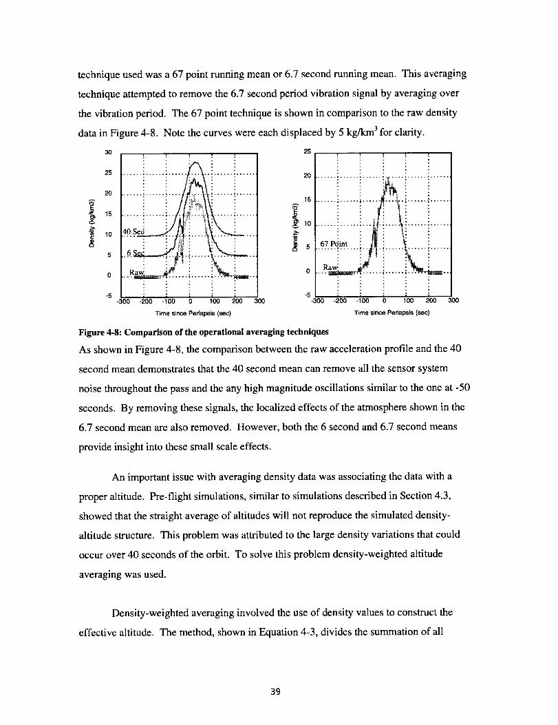
technique used was a 67 point running mean or 6.7 second running mean. This averaging
technique attempted to remove the 6.7 second period vibration signal by averaging over
the vibration period. The 67 point technique is shown in comparison to the raw density
data in Figure 4-8. Note the curves were each displaced by 5 kg/km 3 for clarity.
3O
25
20
15
I0
5
0
-5
40 S
6 : : i .
; ; ; ;-300 -200 -100 0 100 200
Time since Pedaps_ (sec)
3OO
25
2O
15
c• 5o
-5-3oo -_oo -_oo
!
...........;.....A.i......i.................i............M__..
;0 1'00 ;_00 300
Time since Periapsis (sec)
Figure 4-8: Comparison of the operational averaging techniques
As shown in Figure 4-8, the comparison between the raw acceleration profile and the 40
second mean demonstrates that the 40 second mean can remove all the sensor system
noise throughout the pass and the any high magnitude oscillations similar to the one at -50
seconds. By removing these signals, the localized effects of the atmosphere shown in the
6.7 second mean are also removed. However, both the 6 second and 6.7 second means
provide insight into these small scale effects.
An important issue with averaging density data was associating the data with a
proper altitude. Pre-flight simulations, similar to simulations described in Section 4.3,
showed that the straight average of altitudes will not reproduce the simulated density-
altitude structure. This problem was attributed to the large density variations that could
occur over 40 seconds of the orbit. To solve this problem density-weighted altitude
averaging was used.
Density-weighted averaging involved the use of density values to construct the
effective altitude. The method, shown in Equation 4-3, divides the summation of all
39

densityandaltitudeproductsby asummationof thedensitiesover theaveragingrangeto
determinetheaveragedaltitude.
n
E Pi Zii=l
ZAVC -- _ (4-3)
i=l
In Equation 4-3, n is the number of points to be averaged, pi is the density of the ithpoint,
and z_ is the altitude of the i _ point.
4.5 Special Products
Several special products were required by other MGS Project Teams. These
special products included dynamic pressure, free-stream heat flux, ephemeris timing
correction, effective scale height for NAV, and atmospheric disturbance level.
4.5.1 Dynamic Pressure and Free Stream Heat Flux
Dynamic pressure and free stream heat flux were used to evaluate present and
future aerobraking passes for effectiveness and safety. Free-stream heat flux was
calculated to monitor the heating levels in the solar arrays and dynamic pressure was a
metric used to avoid further damage to the crack and to describe the effectiveness of
aerobraking passes. Dynamic pressure and free stream heat flux are both functions of the
density and the velocity of the spacecraft and are calculated using Equation 4-4.
1 2 1 3
q = 2 pv Q = -_ pv (4-4)
In Equation 4-4, q is the dynamic pressure, p is the density, v is the velocity of the
spacecraft and Q is the free stream heat flux.
Note that using the operational data reduction process allowed for calculation of
these two parameters at any time during the drag pass. This allowed the ACC Team to
40

calculatethemaximumheatflux and dynamic pressure during each pass and also calculate
the time of these maximum points in relation to the periapsis of the orbit
4.5.2 Ephemeris Timing Correction
Since the NAV Team would only commit to periapsis timing errors less than 225
seconds [Personal Commun_ication, P. Esposito, 6/96], a method for refining the peripasis
time to within 10 seconds was created. The product, called ephemeris timing correction
(ETC), was the time in seconds from the NAV estimated periapsis time to the time of
actual periapsis assuming a symmetrical atmosphere. A symmetrical atmosphere has no
latitudinal or longitudinal variation, i.e. densities encountered before periapsis are equal to
densities calculated after periapsis. To determine the ETC, the time corresponding to the
accelerometer measurements was shifted until all variation between pre- and post-periapsis
densities were minimized. The amount of time shift which minimizes this variation was the
ETC.
When tested on models with symmetric atmospheres, the ETC process could
detect errors in periapsis time on the order of 1 second. This process was not used during
aerobraking because NAV team timing errors were consistently less than 3 seconds and
average timing errors calculated with ETC were 10 seconds. This lack of accuracy in the
ETC product shows the very non-symmetric nature of the Martian atmosphere.
4.5.3 Effective Scale Height for NAV
As part of the orbit determination process, the NAV team estimated the density at
periapsis using a constant density scale height model of the atmosphere. Since the NAV
team could not determine scale height, a process was generated to use accelerometer data
to estimate a scale height that best describes the entire pass. This scale height was known
as 'Effective Scale Height for NAV'.
The following procedure was used to calculate 'Effective Scale Height for NAV'.
First, the density calculated at periapsis by the accelerometer was assumed to be the
41

correctdensity. Second,thetotalchangein velocityrecordedby theaccelerometer
duringtheentirepasswascalculatedbydeterminingthesumof all individual0.1second
measurements.To correctfor differencesbetweenaccelerationsin thez-directionand
accelerationsalongthevelocityvector,eachaccelerometerpointwasdividedby the
cosineof Ux andUy beforethesummationwastaken. Third,adensityprofilewas
generatedusingaconstantdensityscaleheightmodelwith theaccelerometer-calculated
periapsisdensityandanarbitraryscaleheight. Fourth,Equation3-1wasusedtocalculate
accelerationsovertheentirepassfrom thedensityprofile generatedin stepthreeandthe
NAV constantballistic coefficient(CD=1.99,A=I 7.03). The sumof theaccelerations
from step4 wascomparedto thetotalaccelerationcalculatedin step2. Finally, steps3
and4 arerepeatedchangingthearbitraryscaleheightuntil thedifferencebetweenthe
accelerationin step2andin step4 wasminimized.Thescaleheightwhichminimizesthis
processwasthe 'Effective ScaleHeight for NAV'.
4.5.4 Atmospheric Disturbance Level
To describe the volatility of the atmosphere, a metric was devised so that the
magnitude of changes in density could be compared from pass to pass. The metric, known
as Atmospheric Disturbance Level (ADL), is defined by Equation 4-5.
i=0-5
ADL = 200 * 10a
lOgl0(Pi-l)
loglo(pi) 6
(4-5)
In Equation 4-5, O is the present orbit number and p, is the density of the n thorbit. ADL
examines the 2 sigma percent deviation of the density ratios of 6 previous orbits relative to
the mean density ratio.
42
-rl ]IF

4.6 Prediction Methods
Two basic prediction methods using accelerometer data were developed for MGS
aerobraking: the wave model and the look ahead model.
The wave model was based on the discovery that Mars has two distinct density
peaks on opposite sides of the planet which remain in the same general area over long
periods of time [16]. This discovery was made after a standing wave pattern was
recognized in the density data. To form a prediction model using this discovery, a least-
squares process was used to determine the constants of a standing-wave density model.
The inputs to the least squares process were the densities and the longitudes of a set of
previous orbits. To predict future densities, this model was evaluated at the predicted
longitudes of the future orbits. The wave model used during aerobraking, shown in
Equation 4-6, contains a constant term, a linear term, and standing wave 1 and wave 2
terms. A standing wave 1 is defined as a sinusoidal density variation with a 360 degree
longitude variation and a wave velocity equal to zero. Wave 2 is similarly described
except a full wave 2 has a 180 degree longitude variation.
prnodel= A0 + Alt + A2 cosL + A3 sinL + A4 cos(2L) + A5 sin(2L) (4-6)
In equation 4-6, A0->5 are constants determined from previous orbits, t is time, L is the
longitude and p is the density.
The look-ahead model was based on the assumption that the density over any
latitude will form a consistent density profile independent of time. To calculate
predictions, data from previous orbits at the same latitude as the prediction periapsis were
fit with a constant density scale height atmospheric model. This model was extrapolated
downward to the altitude of the prediction point to determine the density prediction. A
sample diagram describing how the model works is shown in Figure 4-9.
43

141
.--.. 14(
13=
12._
12C
11.=
30
! ! ! ! ! , 15C ......................... :: ; : '':::;
k.l...j........i...._,,,,.._.o.,._ .}./I ,,.,.J..i.iJ.iJJli...J.__::::,_:.o"._:F,,;o......._'\': ! Pred,etion Or_|t _//] " _,:"i _ Past Data at Latitude of
I_..iiii...tl/i_.. .i ........ ::....... i ....... i........ ! ..... t/ !_.],, ,,_ ..._..i._)ii....i..ii.i _'edictionOrbitiiiii i iii!ii! i liii
\\\\.....i.......i.......7........i117;4 _'_ if!iiiJiliiiiiiii....... i ....... •........ i........ . .... '.,)/'.,,/.. 1_ .... i..;.:.._Lii....i.._i.;;i:::,.,.......i.:._i.i...L.i.iiL.i
CMoti_ ! : /_ i"i'i !i!i!!'"i"! i'iiii:: ! i'i'i'iii!i ! ! i iiiii......27/I iiiiiiiiii ii iiiiiiiii!i!iii• i " . _ i i:,.iii":il::iiii!..:..ii:::i:!ii!!-!-:.:.!
: :::__.=- -_. - I, "'!i!i!_i'"_ud!i'i;i!!!!iiii_..;.!i iii!
!'p" i ! i I iiii::::: iiiiiiiMOtion ; i i i I 11_ ...................................
35 40 45 50 55 60 65 10 z 16' 1(_ 10 _ 10
Latitude (deg) Density (kg/krn 3)
Figure 4-9: Look-ahead model diagram
44
11 I-

5. Analysis of Process Errors
Section 5 analyzes the error induced into the calculations of density by the
operational methods described in Section 4. The total induced error can be determined by
the root-mean square of all the possible errors inherent to these methods. These error
sources include:
1. Ephemeris errors
2. Errors in determining ballistic coefficient
3. Errors in determining bias
4. Digitization errors due to the accelerometer instrument
5.1 Ephemeris Errors
Ephemeris errors include errors from the use of periapsis osculating elements away
from periapsis, and timing and altitude errors from orbital elements generated by the NAV
Team. Errors from the use of osculating elements are described in Section 3.2. Timing
error is the amount of time that elapses from the actual periapsis point to the one predicted
by the NAV Team, assuming the orbit is correct. Altitude error is the error in altitude
assuming the timing of periapsis is correct. From discussions with the NAV Team
[Personal Communication, P. Esposito, 6/96], the ephemeris errors in a reconstructed
orbit were estimated at 0.1 km in altitude and 0.1 second in time.
Total altitude error is the combination of the range errors in Section 3.2 and NAV
altitude errors. The equivalent density error was determined by solving the equation of a
standard exponential atmosphere (p= Po exp[zkH/Hs] ) for density ratio, P/9o, assuming a
scale height, Hs, of 7 km and a zSJ-Iof the corresponding total altitude error. The results
of the total altitude error for several altitude ranges are shown in Table 5-1.
45
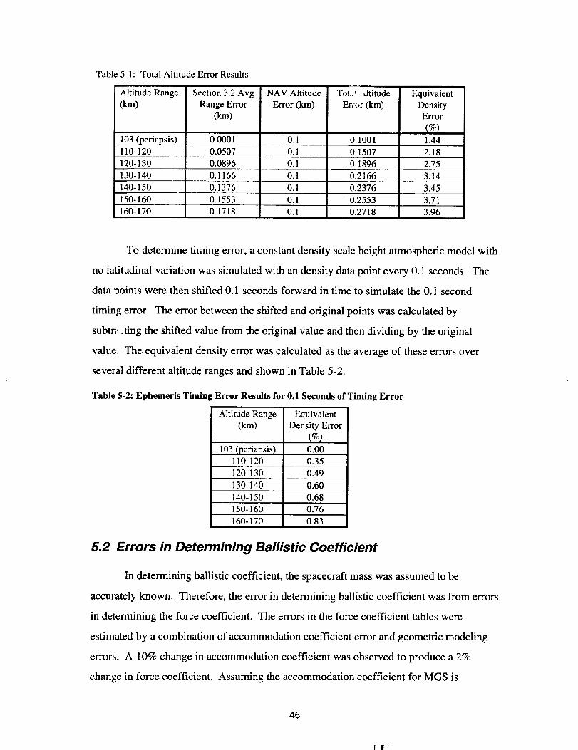
Table 5-1: Total Altitude Error Results
Altitude Range
(gin)
103 (periapsis)110-120
Section 3.2 Avg
Range Error
0.0001
NAV Altitude
Error (kin)
0.0507
120-130 0.0896
To_::i _.ltitude
Er;oc (km)
0.1 0.1001
0.1 0.1507 2.18
0.1 0.1896 2.75
Equivalent
DensityError
1.44
130-140 0.1166 0.1 0.2166 3.14
140-150 0.1376 0.1 0.2376 3.45
150-160 0.1553 0.1 0.2553 3.71
0.1718160-170 0.1 0.2718 3.96
To determine timing error, a constant density scale height atmospheric model with
no latitudinal variation was simulated with an density data point every 0.1 seconds. The
data points were then shifted 0.1 seconds forward in time to simulate the 0.1 second
timing error. The error between the shifted and original points was calculated by
subtr_,:ting the shifted value from the original value and then dividing by the original
value. The equivalent density error was calculated as the average of these errors over
several different altitude ranges and shown in Table 5-2.
Table 5-2: Ephemeris Timing Error Results for 0.1 Seconds of Timing Error
Altitude Range
(km)
103 (periapsis)110-120
Equivalent
Density Error
0.00
0.35
120-130 0.49
130-140 0.60
140-150 0.68
150-160 0.76
160-170 0.83
5.2 Errors M Determining Ballistic Coefficient
In determining ballistic coefficient, the spacecraft mass was assumed to be
accurately known. Therefore, the error in determining ballistic coefficient was from errors
in determining the force coefficient. The errors in the force coefficient tables were
estimated by a combination of accommodation coefficient error and geometric modeling
errors. A 10% change in accommodation coefficient was observed to produce a 2%
change in force coefficient. Assuming the accommodation coefficient for MGS is
46
I |1

between 0.95 and 1.0 results in a 1% error in force coefficient. Error in force coefficient
due to geometric model imperfections was estimated at 2% [Personal Communication, R.
Wilmoth, 9/14/98]. Therefore, the error inherent to the calculation of force coefficient
tables is the root-mean square of the accomodation coefficient and model imperfections
errors or 2.24%. To determine total error in force coefficient, the inputs to the
interpolation of the force coefficient tables, wind orientation and panel deflection, were
also considered.
To calculate the wind orientation error, a 1 degree error in wind orientation was
assumed. The greatest variation in the interpolation tables shows Cz changes from 2.12
for the free molecular table with Ux=Uy=0 to 1.98 for the free molecular table with
Uy= 10 degrees. This constitutes a 0.0134 Cz change per degree of orientation error which
can be used to state that a 1 degree orientation error will cause a 0.65 % error in density
estimation.
For determining error in calculation of panel deflection, the panel position
calculated using methods from Section 4.4.3 and the panel deflection calculated from sun
sensor data were compared. The greatest difference between the two independent
calculations inside the atmosphere is approximately 1 degree. Using a similar method to
the one used above, the greatest variation in the interpolation tables occurs from 2.12 for
the free molecular table, with no panel deflection to 2.0194 for the free molecular table
with 10 degrees panel deflection. This constitutes a 0.01006 Cz change per degree of panel
deflection error which was used to state that a 1 degree deflection error will cause a 0.47
% error in density estimation.
5.3 Errors in Determining Bias
The average standard error in determining the bias was 0.005 counts/0.1 seconds.
By simulating a sample pass using a linear temperature profile described in Section 4.2, the
counts every 0.1 second can be determined at various altitude levels. By assuming a
0.005 counts/0.1 second error on each acceleration value, an error can be identified as a
47

function of acceleration. The equivalent density error is then the average acceleration
error over each altitude interval and is shown in Table 5-3.
Table 5-3: Bias Percent Error as a Function of Count Level
Altitude Range(_n)
103 (periapsis)110-120
AverageAcceleration
(counts/0.1 sec)9.060
2.119
Equivalent DensityError
0.06
0.24
120-130 0.618 0.81
130-140 0.219 2.28
140-150 0.089 5.63
150-160 0.040 12.60
160-170 0.019 25.95
Note that this density error is an orbit-to-orbit variation dependent on the ability to
accurately determine the bias value. Since this error does not vary during the orbit, the
scale heights determined from accelerometer data do not suffer from this error type.
5.4 Errors due to Instrument Output
The accelerometer instrument output suffers from quantization, only integer count
levels can be reported by the instrument, and data rate errors, the same data rate can
produce several permutations of the existing atmosphere. Both of these errors are
determined by the simulations in Section 4.3. The results of the simulation done to
investigate these errors for the 10 measurements per second case are repeated in Table 5-4
as the errors due to the accelerometer instrument output.
Table 5-4: Quantization and Data Rate Error Results
Altitude Range
(km)
103 (periapsis)
110-120
AverageAcceleration
(counts/0.1 sec)
9.060
2.119
Equivalent Density
Error (%)
(10 acceleration
measurements/sec)
0.82
0.89
120-130 0.618 0.44
130-140 0.219 0.79
140-150 0.089 1.85
150-160 0.040 4.37
160-170 0.019 6.84
48
-T]I l-

Note that at approximately 125 km, the accelerometer instrument is recording 1 count
every 0. ! seconds. Without the averaging techniques used in the operational data
reduction procedure, the error due to quantization of the signal at that altitude level
should be 100%, ie the instrument could report 2 or 0 counts instead of 1 count. Table 5-
4 shows that using averaging techniques outlined in this paper reduces this error to
approximately 1%.
5.5 Total Data Reduction Process Error
By combining all the error sources described in Section 5.1 through 5.4, a total
error was generated as a function of altitude and acceleration. The total error was found
by taking the root mean square of all error sources. All the error sources and the total
data reduction process error are shown in Table 5-5.
Table 5-5: Total Data Reduction Process Error
Altitude Average Average Ephemeris Errors Ballistic Coef. Errors Natural Instrument TOTAL
Range Density Acceleration Altitude Timing Force Orientation Panel Bias Output PROCESS
(kin) (kg/km3) (counts/4Os) Error Error Coef. Error Deflectior Error Error ERROR
(%) (%) Error (%} (%) Errorl% / I%1 I%_ (%)
103 (periapsis 60.00 3624 1.44 0.00 2.24 0.65 0.47 0.06 0.82 2.90110-120 13.91 847.6 2.18 0.35 2.24 0.65 0.47 0.24 0.89 3.37
120-130 4.12 247.2 2,75 0.49 2.24 0.65 0.47 0.81 0.44 3.78
130-140 1.46 87.6 3.14 0.60 2.24 0.65 0.47 2.28 0.79 4.66
140-150 0.59 35.6 3.45 0.68 2.24 0.65 0.47 5.63 1.85 7.29
150-160 0.27 16 3.71 0.76 2,24 0.65 0.47 12.60 4.37 14.07
160-170 0.13 7.6 3.96 0.83 2,24 0.65 0.47 25.95 6.84 27.24
The data in Table 5-5 is plotted in Figure 5.1. The left hand side of Figure 5-1
total data reduction process error plotted as a function of altitude and the right
shows the same error as a function of density.
shows the
hand side
49

o_v
LU
9
t-O
t5"O
tr
o
30
25
20
15
10
30
§ 2siii
8 20O.
t-O 15
_ 10
O 5
..... : ..... : ..... : ..... ! ..... : ..... :...
..... ; ..... ; ..... ; ..... ; ..... ; .........
....ii.........[
100 110 120 130 140 150 160 170
• --:::: : : ;:::::: :::::: : : ::::;:
iii!iii i iiiiiii
i iiiiiij i i iliiii
i:!!!!! : :::::::: : • ; ::::
: : : : ::::
] ] iiiiii
o o-110 1o0 101
• • • _Tr..
: : : ::'::
]] ....... ........ ]] ]]]]]]: : : ; :::[ ................: : :::::: : : :::::: : : " :::::
ldDensity (kg/kmAltitude (km)
Figure 5-1: Accelerometer process error vs. model altitude and density
This study demonstrates that accelerometer measurements can be converted to density
with only 5% error for the 33 km range between periapsis at 103 km and 136 km. Higher
altitudes up to 162 km can be examined but 25% uncertainty should be expected. The
total process error can also be examined as a function of density using the right hand side
of Figure 5-1.
An important note is that the total process error developed in this section contains
components that are only correct for the density structure used to generate these errors.
Altitude error, timing error, natural bias error and instrument output error are all functions
of the density and the density change with altitude. Since the density structure used here
was based on a previous aerobraking orbit, the total process error results are typical of
what was experienced during aerobraking at Mars but not indicative of every aerobraking
pass.
50
-1; 11I

6. Verification of Accelerometer Results
Section 6 presents the studies done to verify the accelerometer data reduction
procedure outlined in Section 4. Studies were also performed to verify the effectiveness
of prediction schemes described in Section 4.6.
6.1 Data Reduction Process Verification
To verify the accelerometer data reduction process, two data products were
examined. The first product, SAM panel deflection, was estimated during the density
iteration scheme. The Spacecraft (S/C) Team also calculated panel deflection by using
spacecraft attitude data and data from sun sensors on the SAM. The second product,
change in orbital period, was estimated by the ACC Team and the NAV Team.
6.1.1 Panel Deflection Comparison: ACC vs. Sun Sensor
For all orbits in which SAM deflection angle was calculated using the sun sensor,
the accelerometer calculated panel deflection was always within 1.5 degrees of the sun
sensor data. Four passes are shown as examples of this accuracy. Passes 50, 100, 125
and 162 are shown in Figure 6-1.
51
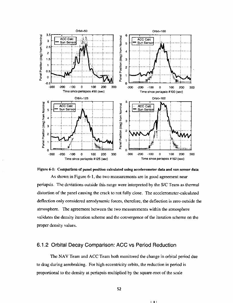
E
EOz
E
"IDv
EO
Oft.
c-
fl..
3.5
3
2.5
2
1.5
1
0.5
0
-0.5
-_ 6
z
E£ 4
8'_3
i213_
E
o,.
0
-300
Orbit=50
i i i ._ i i
I ACCCa,cr :,i_ i :I-- Sun Senso_"i_ i'": ...... i ............ _ ...... :..... _._i _,..: ...... :......
-300 -200 -100 0 1(30 200 300
Time since perlapsis #50 (sec)
Orbit= 125
L = I
I ACC Calc /
"t--Sun Sen_ °_' " " " _,i'" "i ...... i ......
-200 -100 0 100 200 300
Time since periapsis #125 (sec)
-_ 6
E
# 5Eo 4
EO
(/)Ofl_
(t$(L
.-_
.EE
E£
8,
EO
O
19E
0.
Orbit= 100
• , , , ,
n A'CCc_,_/ i i i
__ "_i? ...... i.......
0
-300 -200 -100 0 100 200 300
Time since periapsis #100 (sec)
Orbit= 162
4 I------s.u-_.-sen_-°.l../_i, ,. ............
2 i _ill_3 ..... " ...... :... _2.. i : ...... :- ......
' ......i' 41 . iii0 I _ :
-300 -200 -100 0 100 200 300
Time since perlapsis #162 (sec)
Figure 6-1: Comparison of panel position calculated using accelerometer data and sun sensor data
As shown in Figure 6-1, the two measurements are in good agreement near
pcriapsis. The deviations outside this range were interpreted by the S/C Team as thermal
distortion of the panel causing the crack to not fully close. The accelerometer-calculated
deflection only considered aerodynamic forces, therefore, the deflection is zero outside the
atmosphere. The agreement between the two measurements within the atmosphere
validates the density iteration scheme and the convergence of the iteration scheme on the
proper density values.
6.1.2 Orbital Decay Comparison: ACC vs Period Reduction
The NAV Team and ACC Team both monitored the change in orbital period due
to drag during aerobraking. For high eccentricity orbits, the reduction in period is
proportional to the density at periapsis multiplied by the square-root of the scale
52
1-11

height.[17] The product was used as a metric to compare drag calculations by the NAV
Team and the ACC Team. In Figure 6-2, the P_s product generated by NAV Team data
was compared against the same product composed of the accelerometer calculated density
at periapsis and the Effective Scale Height for NAV for orbits 140 to 200. Below the
P_/-_-s product plot in Figure 6-2 is the error between the two calculations.
,oo ...........i.............i.........i-"--_iXvii.............i........................',..................... ............__.-,_"_"t!_.......,,_....!-ii:l.........................._._._°.!:!._.'.y_ _.__,._._:.,._ ....
_:_ _-_ f :_ _!_ _ i_: /. _" : _ t.'/_'i I..... ............:....\...' : : "_ i " : _-_
60
40
20 ............. :............. -"............. :........................... :.........i
z
L)L)<
z
o
0
-0.1
-0.2
-0.3
............. i
140 150 160 170 180 190 200Orbit Number
Figure 6-2: Orbital decay comparison of NAV and ACC using P_s product
As shown, the ACC Team estimate of the P_s product was on average 5% below the
NAV Team estimate. This error was believed to be due to the differences between the
constant drag coefficient used by the NAV Team (1.99) to calculate periapsis density and
the variable force coefficient used by the ACC Team to calculate periapsis density. If the
percent difference is calculated between the NAV coefficient of drag number of 1.99 and
the average force coefficient near periapsis determined for this orbit range of 1.9, the 5%
results. The ability to exactly reproduce the P,_-s product generated by the NAV Team,
validates the periapsis densities determined by the accelerometer data reduction process
53

andthemethodfor isolatingaccelerationdueto aerodynamicforcesfrom themeasured
accelerationovertheentirepass.
The 'Effective ScaleHeight for NAV' productwasalsovalidatedusingthe
px/-H-_-sproduct. Two simulation runs of aerobraking passes were made, first with the NAV
Team scale height and then with the ACC Team effective scale heights. The results of
these tests are shown in Table 6-1 [Personal Communication, P.Esposito, 12/11/97].
Table 6-1: Results of NAV Simulation Runs with Aecelerometer Calculated Effective Scale Height
Pass
NumberNAV Scale
Height
7.0
NAV DensityUsing NAV Hs
ACC Effective
Scale Height
NAV DensityUsing ACC Hs
59 8.83 11.5 6.92
60 7.0 12.90 6.21 13.55 14.60
ACCCalculated
Density7.23
Comparing the NAV density calculated using the NAV scale height to the ACC density
values resulted in a 22% error for pass 59 and a 12% error for pass 60. If the NAV
density is re-calculated using the ACC effective scale height, the error between NAV
density and accelerometer density was reduced to 4% for pass 59 and 7% for pass 60.
This demonstrates not only the dependence of the NAV Team on proper scale height
information but how much improvement can be made on orbit determination when a more
precise calculation of scale height can be made.
6.2 Prediction Scheme Verification
To verify the prediction methods, densities of previous passes were predicted and
compared to the actual density calculated for that orbit. Prior to aerobraking the MGS
project estimated the variability inherent to the Martian atmosphere at a two sigma value
of 70%. Therefore, an accurate prediction method is one that could consistently predict
upcoming densities below this variability value.
Several prediction schemes were used during aerobraking. These schemes
included: Persistence, which used scale height and density of the previous pass to predict
one orbit ahead; 5-Orbit Mean, which used 5 previous densities, scaled to the
54
:ll !
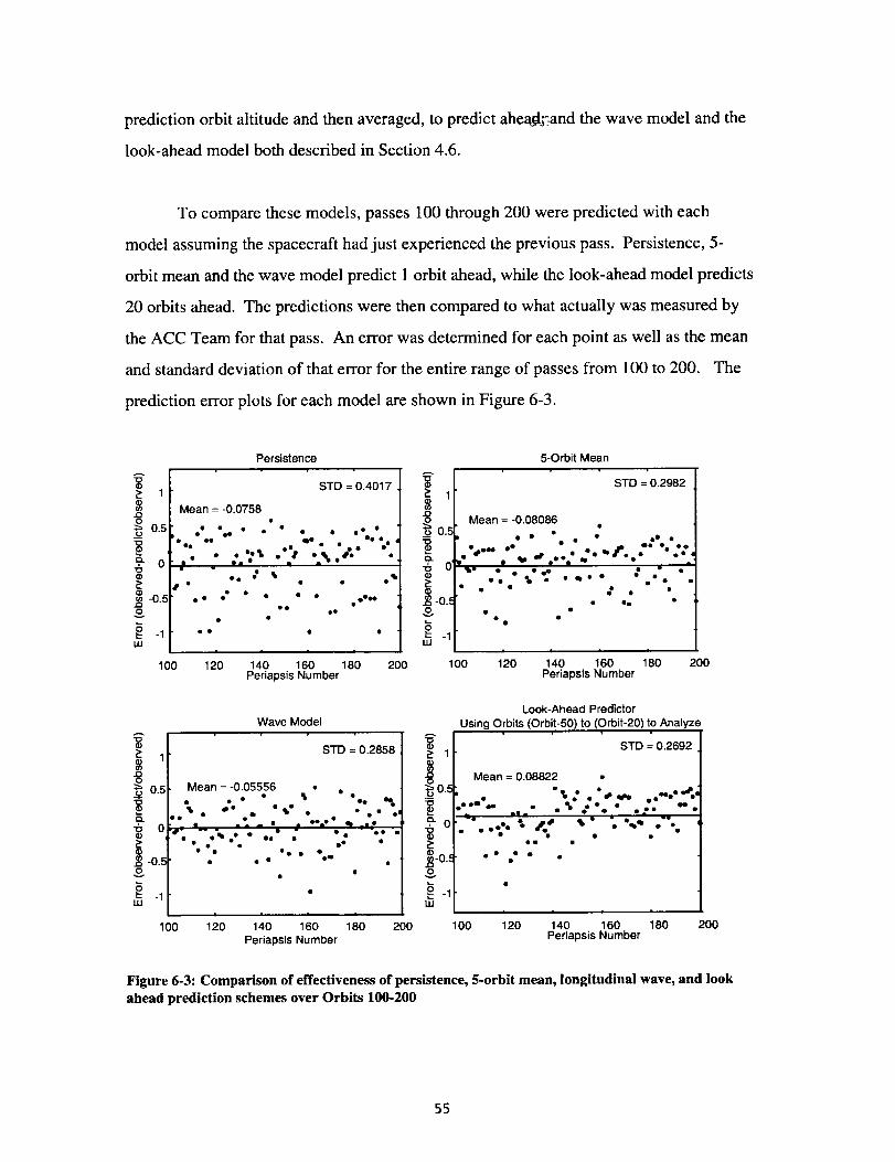
prediction orbit altitude and then averaged, to predict ahea_d;3and the wave model and the
look-ahead model both described in Section 4.6.
To compare these models, passes 100 through 200 were predicted with each
model assuming the spacecraft had just experienced the previous pass. Persistence, 5-
orbit mean and the wave model predict 1 orbit ahead, while the look-ahead model predicts
20 orbits ahead. The predictions were then compared to what actually was measured by
the ACC Team for that pass. An error was determined for each point as well as the mean
and standard deviation of that error for the entire range of passes from 100 to 200. The
prediction error plots for each model are shown in Figure 6-3.
Persistence
Mean = -0.0758JDO •
oe oe • o_
-0,5 0o 00 " " " "Q • • • o°°°0 o•
-I " "
t_l , l
100 120 140 160 180Periapsis Number
STD = 0.4017
5-Orbit Mean
_" STD = 0.2982
1
Mean = -0.08086_ 0.5 • "
• i
, 0 _ e I . -
• ''e % • . e_ • •(D • _ •
• o: •
O "_ • •
• _ -1
UJ
200 1O0 120 140 160 180 200Periapsls Number
JDO
0.5
0(9
-o.5o
-1LU
Wave Model
STD = 0.2858
Mean = -0.05556
-....;. . '.-..-.". .. .,c z.
• • • • •o• o• •
• • • °oil •
00
_0..=
_-0.5
UJ
Look-Ahead Predictor
Using Orbits (Orbit-50) to (Orbit-20) to Analyze
STD = 0.2692
Mean = 0.08822 •
• 0% ? • od, _', •., ,,_,•g " •
o• ,De • • • o• o° ° o • • •e e• i
. "..oo'o °o o_oo_p qlJl • ".'.. • .
• • ° • •
|
100 120 140 160 180 200 100 120 140 160 180 200
Periapsis Number Perlapsis Number
Figure 6-3: Comparison of effectiveness of persistence, 5-orbit mean, longitudinal wave, and look
ahead prediction schemes over Orbits 100-200
55
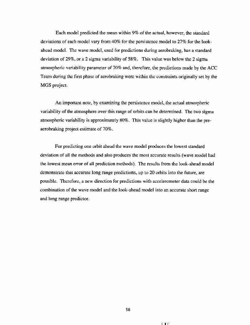
Each model predicted the mean within 9% of the actual, however, the standard
deviations of each model vary from 40% for the persistence model to 27% for the look-
ahead model. The wave model, used for predictions during aerobraking, has a standard
deviation of 29%, or a 2 sigma variability of 58%. This value was below the 2 sigma
atmospheric variability parameter of 70% and, therefore, the predictions made by the ACC
Team during the first phase of aerobraking were within the constraints originally set by the
MGS project.
An important note, by examining the persistence model, the actual atmospheric
variability of the atmosphere over this range of orbits can be determined. The two sigma
atmospheric variability is approximately 80%. This value is slightly higher than the pre-
aerobraking project estimate of 70%.
For predicting one orbit ahead the wave model produces the lowest standard
deviation of all the methods and also produces the most accurate results (wave model had
the lowest mean error of all prediction methods). The results from the look-ahead model
demonstrate that accurate long range predictions, up to 20 orbits into the future, are
possible. Therefore, a new direction for predictions with accelerometer data could be the
combination of the wave model and the look-ahead model into an accurate short range
and long range predictor.
56
qll-

7. The Effect of Panel Vibration on MGS and the
Accelerometer Data Reduction Process
The vibration of the SAM panel has contributed a 6.7 second period oscillating
signal to the acceleration. Three methods were developed to remove this signal:
averaging described in Section 4.4.4, the 4-DOF dynamics model described in Section
3.1.7, and a filtering process.
The filtering process used band-pass filtering to isolate the 6.7 second period
signal in the accelerometer data. The filtered signal can then be subtracted from the
measured acceleration to remove the effects of panel vibration. To quantify the band-pass
filtered signal a least-squares process was then used to obtain the constants in Equation 7-
1 which described the oscillating component of the acceleration data in terms of the
oscillating components of the rates and angular accelerations.
azBp = ClCOx + C20C, x (7-1)
In Equation 7-1, azBp is the acceleration in the spacecraft z-direction due to panel
vibration, COxis the angular rate in the spacecraft x-direction filtered with a similar band-
pass as above, Ctx is the band-pass filtered angular acceleration in the spacecraft x-
direction, and C1 and C2 are the constants determined in the least squares process.
This section will describe the effectiveness of the 4-DOF dynamics model in
determining the oscillating component of the acceleration data, Since the results from the
model do not exactly agree with results from the filtering process, sensitivity studies were
performed to determine which combinations of spacecraft and SAM physical properties
could make the two methods agree. Finally, the effectiveness of averaging techniques
used to compensate for the panel vibration signal are determined by comparing the results
of the 4 DOF dynamics model method to several different averaging techniques.
57
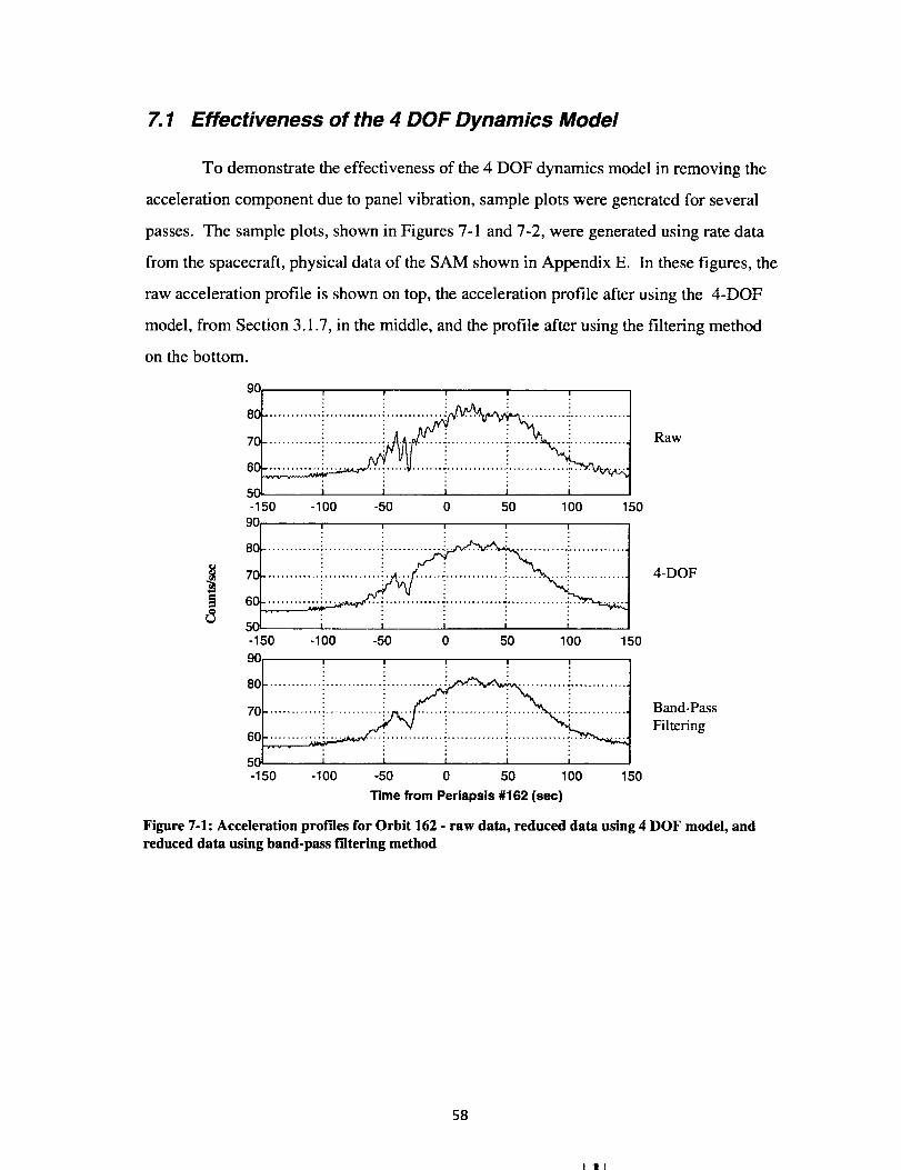
7.1 Effectiveness of the 4 DOF Dynamics Model
To demonstrate the effectiveness of the 4 DOF dynamics model in removing the
acceleration component due to panel vibration, sample plots were generated for several
passes. The sample plots, shown in Figures 7-1 and 7-2, were generated using rate data
from the spacecraft, physical data of the SAM shown in Appendix E. In these figures, the
raw acceleration profile is shown on top, the acceleration profile after using the 4-DOF
model, from Section 3.1.7, in the middle, and the profile after using the filtering method
on the bottom.
9C
8C
7C
6c
5C
90 ! ! ! ! !
__80............"i.............i............._ ! ...........i.............70 ............::.............i....... i.............
-150 -100 -50 0 50 100 150
I I l I I
iiiiiiiiiili::ili:::.......'........i:ili:ii::iiiii-150 -100 -50 0 50 100 150
9O
70 _ ......... i .........60-
50 I I I I ,-150 -100 150-50 0 50 100
Time from Perlapsis #162 (sec)
Raw
4-DOF
Band-Pass
Filtering
Figure 7-1: Acceleration profiles for Orbit 162 - raw data, reduced data using 4 DOF model, and
reduced data using band-pass rdtering method
58
=1 Ill
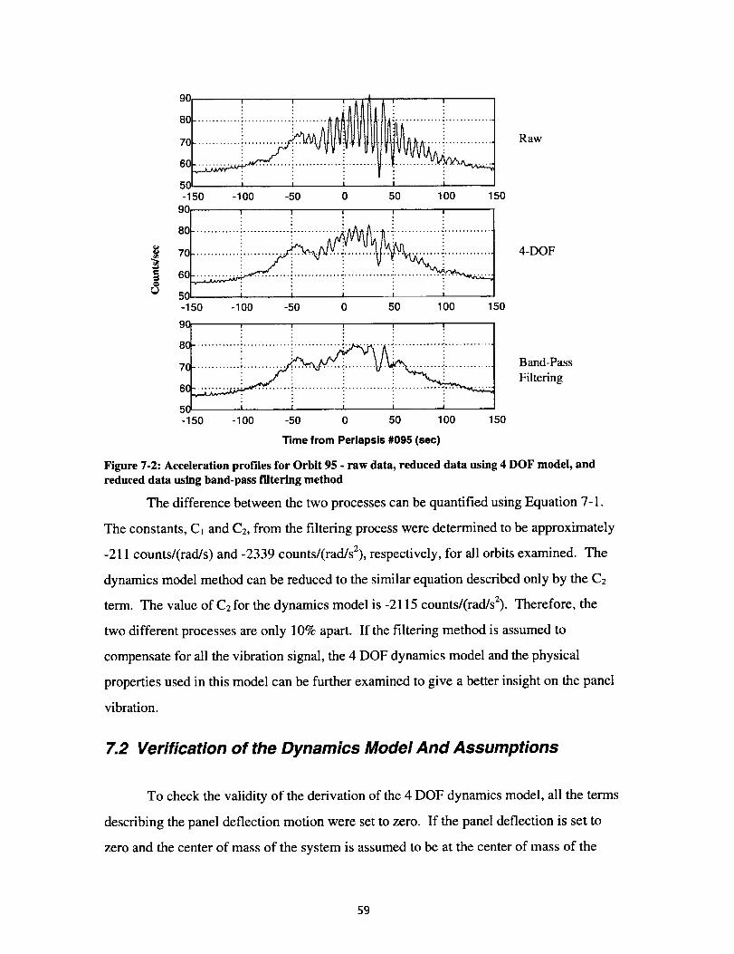
70
| 60
9C
iiiiiiiiiilliiiiii..........: ........iiiiiiiii iiiii6C
5C i i t = i-150 -100 -50 0 50 100 50
90 ! ! ! ! !
50 I , , = '-150 -100 -50 0 50 100 150
9C ! ! ; ! :
8C :_
7C
6C
5C i , i =-150 -100 -50 0 50 100 150
Time from Periapsis #095 (sec)
Raw
4-DOF
Band-Pass
Filtering
Figure 7-2: Acceleration profiles for Orbit 95 - raw data, reduced data using 4 DOF model, and
reduced data using band-pass _tering method
The difference between the two processes can be quantified using Equation 7-1.
The constants, Cl and C2, from the filtering process were determined to be approximately
-211 counts/(rad/s) and -2339 counts/(rad/s2), respectively, for all orbits examined. The
dynamics model method can be reduced to the similar equation described only by the C2
term. The value of C2 for the dynamics model is -2115 counts/(rad/sZ). Therefore, the
two different processes are only 10% apart. If the filtering method is assumed to
compensate for all the vibration signal, the 4 DOF dynamics model and the physical
properties used in this model can be further examined to give a better insight on the panel
vibration.
7.2 Verification of the Dynamics Model And Assumptions
To check the validity of the derivation of the 4 DOF dynamics model, all the terms
describing the panel deflection motion were set to zero. If the panel deflection is set to
zero and the center of mass of the system is assumed to be at the center of mass of the
59

BUS+SAP body, the C2 constant determined by the combined process of the dynamics
model and the angular method, outlined in Section 3.1.7, should result in the same C2 if
only the angular method, outlined in Section 3.1.5, is used and the center of mass of the
system is assumed to be at the center of mass of the spacecraft. When the panel deflection
terms were set to zero, the C2 values determined were equal to each other. The
spreadsheet demonstrating this calculation is shown in Appendix F.
To validate the small angles assumption, the panel deflection and the spacecraft
angular position about the spacecraft x-axis were further examined. The panel deflection
exceeded 5 degrees under the normal effects of the atmosphere. However, the vibration
amplitude never exceeded 1 degree off this quasi-steady state defection. The same
properties were observed in the spacecraft x-axis angular position. Therefore, the
deflection angle and the x-axis angular position exceeded small angles but the vibrating
components of these generalized coordinates did not. Since the 4 DOF dynamics model is
only concerned with the vibrating components of these coordinates the small angle
approximation is valid.
To validate the 'no external forces' assumption, the atmospheric force on the two
bodies was further examined. The force of the atmosphere on the panel and the remaining
part of the spacecraft were different due to the different surface areas. However, this
force difference did not oscillate with the 6.7 second period vibration signal. The
oscillation of the atmospheric force would be too low a frequency to affect the short
period oscillation of the damaged panel. Therefore, if the two oscillations never affect
each other, the no external forces assumption is valid.
A unique problem arises when the 4 DOF dynamics model is modified to examine
the effect of external forces on the spacecraft. To determine the external forces on the
spacecraft, the density and the force coefficients must be known. However, the
accelerometer data used to determine density contains the vibration. By adding external
forces to the equation, the vibration would be added twice to the problem. To apply
60
-'VI I "
external forces to the model, the forces must be determined by the aerodynamic forces
alone. Band-pass filtering of the accelerometer data may reveal accelerations due to the
aerodynamics alone, however, the filtering process may also remove the data necessary to
show that the natural oscillations of the atmosphere and of the damaged panel are
resonating and amplifying the vibration of the panel.
7".3 Sensitivity Studies on Panel Physical Parameters
Assuming the dynamics model outlined in Section 3.1.7 is valid, sensitivity studies
were performed to analyze the effect of modifying the physical properties used in the
dynamics model. The properties used in the sensitivity study were the mass of the broken
SAM section, the moment of inertia of the SAM broken section, the center of mass
position of the broken SAM section, and the yoke crack position. Except for crack
position, each of these studies were performed by modifying the individual parameters
mentioned above without disturbing the other parameters. For crack position,
parameters were generated by choosing a position for the crack and then modifying the
other parameters (SAM mass, SAM moment of inertia, and SAM center of mass) so that
the crack position described the object which is vibrating. Table 7-1 describes the position
of the crack and the resulting physical parameters used in the crack position sensitivity
study. In Table 7-1, position #2 corresponds to the position of the hinge between the
yoke and the panel and position #4 corresponds to the best estimate of the crack position
by Lockheed Martin Astronautics (LMA).
Table 7-1: Crack-Line Position and Resulting Physical Parameters for Sensitivity Study
Position
#
SAM mass
kg22.174
2 (hinge) 27.8963 33.618
4 (LMA) 39.3445.062
SAMCG
x y z-0.032 -2199 2.473
-0.023 -2.79 2.339
-0.015 -2.59 2.204
-0.006 -2.39 2.070.003 -2.18 1.936
Ixx SAM
kg-m238.2325
47.09
55.947564.805
73.6625
Hinge Pos
x y0.038 -1.52
0.038 -1.31
0.038 -1.11
0.038 -0.90.038 -O.7
Z
1.49
1.355
1.221
1.0860.952
The trends developed from the sensitivity studies of SAM moment of inertia, SAM
mass, SAM center of mass and crack position are shown below in Figures 7-4
61

through7-7. C2 is used as a metric to describe the effect of modifying the physical
parameters on the dynamics model. In each figure, C2 is shown as a function of the
modified physical parameter. Also shown on each figure is a line demonstrating C2 from
the filtering method. This line represents the physcial parameters necessary to make the
4 DOF dynamics model rcproduce the same results as the filtering method.
-2000
¢:-!OO
(%1
t.3
-2050
-2100
-2150
-2200
-2250
-2300
-2350
-2400
-2450
-2500
20
......................... !..iiiiiii".............. • ............. KI .............. ° ...........
I...... _ .... I(LMAestimate of I
....... SAM properties) I_"" C2= "2339 (filtering method goal) .......................... _.............
............... • .............. # ............. i .............
............... :.............. ; ............. ; ............................. ; ..............
i ; ; i30 40 50 60 70 80
SAM Ixx (samcom) (kg-m2)
Figure 7-3: Sensitivity study on SAM moment of inertia about the spacecraft x-axis at the SAMcenter of mass
-1500
: : : ." ." [-1600 ....... .......... , ........ ; ........ _ ........ "........ : ........ _ ....... ; ........ : ........
i i i i ISAM mass=39.341 i i i [
_ -2000
_ -2200 -
i i
-2400 i 1 I i i i i_ i i t0 5 10 15 20 25 30 35 40 45 50
SAM Mass (kg)
Figure 7-4: Sensitivity study on SAM mass
62
I-| l-

-2000
A
c-
oo
-2O50
-2100
-2150
-2200
-2250
-2300
-2350
-2400
1.3
............. ::............ il SAM CG Position, " r/Y_'" "i ........... i ...........
............ i............ iI k=1.77 (LMA estimate of r....., i ............ i ...........: iI SAM properties) | i i
a ............ •............ i ............ -............ • ...........
............. • ............ ! ............ -............ _ ............ •............ # ...........
C2= -2339 (filtering method goal)n u l
............. •............ ! ............ ............. ,: ............ :............ ,;...........
i i i i i i1.4 1.5 1.6 1.7 1.8 1.9
Distance from SAM CG to Failure Line, (m)
Figure 7-5: Sensitivity study on SAM center of gravity position
A
O4
c-
oo
-1900
-1950
-2000
-2050
-2100
-2150
-2200
-2250
-2300
-2350
-2400
............... i.............. ":.............. .".............. ."
I I I I
0 1 2 3 4 5
Position #
Figure 7-6: Sensitivity study on crack-line position
From examining the four studies above, it can be shown that only unrealistic
modifications to the SAM moment of Inertia, SAM mass, SAM center of mass position,
or crack position will allow the dynamics model to agree with the filtering method. If the
dynamics model is assumed to be correct, this data demonstrates that something else may
be moving on the spacecraft with the same vibration frequency as the damaged panel.
63

7.4 Averaging Techniques Used to Compensate for VibratingPanel Effects
Before the development of the 4 DOF dynamics model or the filtering process,
accelerometer fluctuations due to panel vibration were compensated for by various
averaging techniques described in Section 4.4.4. The comparison can now be made
between what is presently believed to be the aerodynamic acceleration and what was
believed to be the aerodynamic acceleration during aerobraking. Figure 7-7 demonstrates
the comparison between the acceleration profile developed using the 4 DOF dynamics
model and the profile developed using averaging for Pass 162. The graph on the left in
Figure 7-8 is the comparison between the 4 DOF dynamics model (gray line) and the 40
point running mean averaging technique (black line). The graph on the right in Figure 7-7
is the comparison between the 4 DOF dynamics model (gray line) and the 6 point running
mean averaging technique (black line).
3Cm 30
i i012 .................. _......... _. :_.i ......... i ........
1 ......... ",.......... i....... i ........
"_ • .7 .oI ......... i.......... i _ .; ........
1_(_ _ 100 50 0 50 100 150 I 150
TimesincePeriapsis(sec) TimesincePeriapsis(sec)
Figure 7-7: Comparision between 4 DOF dynamics model and 40 pt (left) and 6 pt running means(right) for Orbit 162
Figure 7-7 shows that the 40 point average accurately describes the general trend
of the overall pass and the 6 point average describes the small effects of the atmosphere as
originally planned. Most importantly, Figure 7-7 shows that averaging of data is the
simplest method to compensate for unwanted vibrations in the accelerometer signal.
64

8. Conclusions
Aerobraking is a low-cost technique which was employed during the MGS mission
and will be used on many upcoming missions. To effectively aerobrake, the density which
the spacecraft encounters on every aerobraking pass must be known. No accurate density
models had been created for the Martian atmosphere at the time of MGS, therefore, the
MGS project was dependent on densities estimated by operational methods to plan the
altitudes at which aerobraking would occur. Aerobraking at Mars was made even more
complex and risky by the malfunction of one of the two solar arrays during initial
deployment.
The MGS Accelerometer Team, formed at George Washington University, used an
operational data reduction procedure to estimate densities given acceleration data from an
on-board accelerometer instrument. This paper has described the operational data
reduction procedure and has also described two methods used to predict the densities of
upcoming orbits. These density estimations and predictions formed the basis for the
planning of aerobraking altitudes during the first 201 orbits of MGS aerobraking. In
addition, the operational data reduction procedure has provided the density data necessary
for 1) the discovery of two longitudinal density bulges on opposite sides of Mars and 2)
the first record of the effects of a dust storm on the density of the Martian neutral upper
atmosphere.
The operational data reduction procedure was developed around an iterative
process which determines density by calculating the deflection of the damaged solar array
and a variable force coefficient which accounts for aerodynamic flight regime, spacecraft
orientation and solar array deflection. This procedure has been demonstrated to determine
densities up to 33 km above periapsis in 7 minutes (approximately 1/20 th of 2 hour time
period allotted for MGS operational density analysis). The possible errors over this
altitude range were determined to be less than 5% by considering the total density
65

errorfrom ephemeriserrors,errorsin forcecoefficientandinstrumenterrors. The
accuracyof thisprocedurehasalsobeenverifiedby comparingthesolararraydeflection
andorbitalperiodreductioncalculatedby thisprocedureto independentcalculations
performedby otherMGS TeamsincludingtheNavigationandSpacecraftTeams.
Thedamagedsolararraydeflectedandvibratedeachpassthroughtheatmosphere,
producinganoscillatingsignalin theaccelerometerdata.To analyzeandremovethis
signal,threemethodsweredeveloped:averaging,band-passfiltering anda4 degreeof
freedomdynamicsmodel. By usingtheaveragingmethod,theanalysisof accelerometer
datawasnot affectedby thisvibration. By comparingtheremainingtwo methods
developedto analyzethevibrationsignal,agreaterunderstandingof thedynamicsof the
panelandthespacecraftwasestablished.The4 degreeof freedommodelsuccessfully
compensatedfor 90%of vibrationsignaldeterminedby thefiltering process.Sensitivity
studies,performedto determinethesourceof theoutstanding10%,revealedthatthe
remainingsignalmaybedueto externalforcesnotrepresentedin themodeloranother
componentonthespacecraftmovingatthesamevibrationfrequencysuchasfuel sloshing.
66
-1|1 -

References
[ 1]- "Mars Global Surveyor Fact Sheet", Jet Propulsion Laboratory Publication, JPL 410-
44-2, Dec 1994.
[2]- Dallas, S. Sam, "Mars Global Surveyor Mission." Presented at the 1997 IEEE
Aerospace Conference, Snowmass at Aspen, CO, 1997. Vol. 4, pp173-189.
[3]- Lyons, D.T., "Aerobraking Magellan: Plan Versus Reality," AAS-94-118, 1994.
[4]- Tolson, R.H., et al., "Magellan Windmill and Termination Experiments," Spaceflight
Dynamics, CNES June 1995 Conference, Toulouse, France.
[5]- Keating, G.M. et al., "Models of Venus Neutral Upper Atmosphere: Structure and
Composition," Adv. Space Res. Vol. 5, No. 11, 1985 pp 117-171.
[5]- Shane, R.W. and Tolson, R.H., "Aerothermodynamics of the Mars Global Surveyor
Spacecraft," NASA/CR-1998-206941, March 1998.
[7]- Wilmoth, R.G. et al., "Rarefied Aerothermodymanic Predictions for Mars Global
Surveyor," To be published in the Journal of Spacecraft and Rockets.
[8]- Kahn, R. et. al., _ H.H. Kieffer, B.M. Jakosky, C.W. Synder, M.S. Matthews,
Eds., Univ. of Arizona Press, Tucson, 1992. Pp 1017-1053. Martin, L.J. and Zurek,
R.W., Journal of Geophysical Research, 97, 3221, 1993.
[9]- Lyons, D. T. et al., "Mars Global Surveyor: Aerobraking Mission Overview." To be
published in the Journal of Spacecraft and Rockets.
[ 10]- Diamond, P.S. and Tolson, R.H., "A Feasibility Study of a Microgravity
Enhancement System for Space Station Freedom." AAS Paper 93-626, August
1993.
[11]- Larson, W. J. and Wertz, J.R., Space Mission Analysis and Design, Microcosm Inc,
CA, 1992.
[12]- Meirovitch, L., Methods of Analytical Dynamics, McGraw-Hill Inc., 1970.
[13]- Cestero, F.J. and Tolson, R.H., "Magellan Aerodynamic Characteristics During the
Termination Experiment Including Thruster Plume-Free Stream Interaction."
NASA/CR- 1998-206940, March 1998.
[14]- Henderson, D. M., '_Euler Angles, Quaternions, and Transformation Matricies -
Working Relationships," NASA TM-74839, JSC- 12960, July 1977.
67

[15]- Blanchard, R.C. and Walberg, G.D.. "Determination of the Hypersonic-
Continuum/Rarefied-Flow Drag Coefficient of the Viking Lander Capsule I Aeroshell
from Flight Data." NASA Technical Paper 1793, Dec 1980.
[16]- Keating G.M., Cancro G. J., et al., "The Structure of the Upper Atmopshere of
Mars: In-Situ Accelerometer Measurements from Mars Global Surveyor," Science,
Vol. 279, March 13, 1998, pp 1672-1676.
[17]- King-Hele, D., "Satellite Orbits in an Atmosphere: Theory and Applications,"Blackie and Sons, Ltd, 1987.
68
Tli i¸7
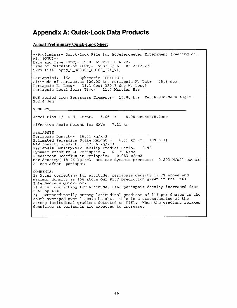
Appendix A: Quick-Look Data Products
Actual Preliminary Quick-Look Sheet
--Preliminary Quick-Look File for Accelerometer Experiment (Keating et.
al.) (GWU)--
Date and Time (UTC)= 1998- 65 TII: 0:6.227
Time of Calculation (EST)= 1998/ 3/ 6 8:2:12.270
OPTG file: optg i 980305 ODI61 171_Vl;
Periapsis#= 162 Ephemeris (PREDICT)
Altitude of Periapsis= 120.00 km, Periapsis N. Lat=
Periapsis E. Long= 39.3 deg( 320.7 deg W. Long)
Periapsis Local Solar Time= 11.7 Martian Hrs
55.3 deg,
MGS Period from Periapsis Elements: 13.80 hrs Earth-Sun-Mars Angle:
202.4 deg
RESULTS
Accel Bias +/- Std. Error: 5.66 +/- 0.00 Counts/0.1sec
Effective Scale Height for NAV= 7.11 km
PERIAPSIS
Periapsis Density: 16.71 kg/km3
Estimated Periapsis Scale Height = 6.11 km (T: 109.6 K)
NAV Density Predict = 17.36 kg/km3
Periapsis Density/NAV Density Predict Ratio= 0.96
Dynamic Pressure at Periapsis = 0.179 N/m2
Freestream Heatflux at Periapsis= 0.083 W/cm2
Max density( 18.96 kg/km3) and max dynamic pressure( 0.203 N/m2) occurs
22 sec after periapsis
COMMENTS:
I) After correcting for altitude, periapsis density is 2% above and
maximum density is 16% above our P162 prediction given in the PI61
Intermediate Quick-Look.
2) After correcting for altitude, P162 periapsis density increased from
PI61 by 41%.
3) Extraordinarily strong latitudinal gradient of 11% per degree to the
south averaged over 1 scale height. This is a strengthening of the
strong latitudinal gradient detected on PI61. When the gradient relaxes
densities at periapsis are expected to increase.
69

Line by Line Description of Preliminary, Accelerometer Quick-Look Sheet
Line
1
2
3
4
5
6
6
10
11
11
12
13
14
15
15
16
17
18
19
20
21
22
23
24
25
27
28
Va/ue
title
Date and Time (UTC) •
Time of Calculation (EDT)OPTG filename
blank
Periapsis#
Ephemeris
Altitude of Periapsis
Periapsis N. Lat
Periapsis E. Long
Periapsis Local Solar Time
Description
Time of Periapsis Passage
Eastern Daylight Time which sheet was created
Name of NAV file used to generate orbit data
Number of Periapsis used in Analysis
Describes the type of NAV product used to develop
QuickLook: (PREDICT, INTERMEDIATE, FINAL)
Geodetic Altitude of SIC periapsis in degrees
Geodetic North Latitude of SIC Periapsis in degrees
East Longitude of SIC in degrees, developed using Mars pole
parameters in OPTG at Date and TimeLocal Solar Time of S/C in hours measure from real sun
subsol point at Date and Time (24 hours/day) (Midnight -
>LST=0.0)blank
MGS Period from Periapsis Orbital period developed using periapsis orbital elementsElements
Earth-Sun-Mars Angle
blank
subtitle
blank
Accel Bias +/- Std. Error
blank
Effective Density Scale Heightfor NAV
blank
subtitle
Periapsis Density
Estimated Periapsis Scale
Height
NAV Density Predict
Periapsis Density/NAV
Density Predict Ratio
Dynamic Pressure at Periapsis
Freestream Heatflux at
Periapsis
Max density Occurrence
blank
Comments
Angle between the Earth and Mars using the Sun as the
middle point
Accelerometer Instrument Bias and Standard Error
calculated by averaging accelerometer values above the
atmosphere before the start of the drag pass
Density Scale Height in km corresponding to a spherically
symmetrical atmosphere with a constant temperature. SeeSection 4.5.2
Density at periapsis
Temperature and scale height in close proximity to periapsis
Density estimation at periapsis from NAV
Ratio of Accelerometer density and NAV Predicted densityRATIO=Line 19 / line 21
Dynamic Pressure at Periapsis in N/m2
DYN. Press.=l/2*density (line 18) *Periapsis Velocity.**2Freestream Heatflux at Periapsis in W/cm2
Qdot=l/2*density (line 18) *Periapsis Velcoity.**3
Density, dynamic pressure and time of maximum density in
reference to periapsis time
Human analysis of 'Quick-Look' data
70
-11 I-

Actual Intermediate Quick-Look Sheet
--Intermediate Quick-Look File for Accelerometer Experiment (GWU)--
Date and Time (UTC)= 1998- 65 TII: 0:6.356Time of Calculation (EST)= 1998/ 3/ 6 12:12:11.220
OPTG file: optg i 980305_ODI61_I71_VI;
Periapsis#= 162 Ephemeris (INTERMEDIATE)
Altitude of Periapsis= 120.00 km, Periapsis N. Lat=
Periapsis E. Long= 39.3 deg( 320.7 deg W. Long)
Periapsis Local Solar Time= 11.7 Martian Hrs
55.3 deg,
MGS Period from Periapsis Elements: 13.80 hrs Earth-Sun-Mars Angle=
202.4 deg
RESULTS
Accel Bias +/- Std. Error= 5.66 +/- 0.00 Counts/O.isec
Effective Scale Height for NAV= 7.05 km
Effective Density (kg/km3)
Scale Height (km)
Estimated Temperature (degK)
Dynamic Pressure (N/m2)
Freestream Heatflux (W/cm2)
Density/5-orbit mean
Scale Height/5-orbit mean
Altitude of 1.26 nbar level(km)
Atmospheric Disturbance Level(2sig%)
Periapsis
16.76
6.06
108.7
0.179
0.083
115.6
INbound [ OUTBound
130____1.52
5.23
93.8
0.59
0.70
123
I01.7
130km_5.52
6.60
118.4
1.33
0.83
132
54.6
Max density( 18.97 kg/km3) and max dynamic pressure( 0.203 N/m2) occurs
22 sec after periapsis
NAV Intermediate Density Solution = 15.66 kg/km3
Periapsis Density/ NAV Intermediate Density Solution Ratio= 1.07
LATITUDINAL VARIATION
[ 61.3 N. Lat (LST= 11.77 hrs, SZA= 85.08 deg) / 48.0 N. Lat (LST=
11.59 hrs, SZA= 71.88 deg)]Altitude= 130.00 km
Density Ratio= 0.28
Density Scale Height Ratio= 0.79
Delta Atmospheric Temperature= -24.64 K
COMMENTS:
i) We predict the following periapsis densities and dynamic pressures
over the next 7 passes (uncertainties are +116 %/- 54 %). Periapsis
altitudes and longitudes were obtained from optg_i_980305_OD161_171_Vl;
Periapsis 151 through 162 were considered in the analysis.
Periapsis_i__Alt (km)__l__E. Long(deg)__i_Density(kg/km3) 1_DynPres(N/m2)
120.43120 73
121 14
121 17120 97
120 78120 76
163
164
165
166
167
168
169
-164 00
-6 31
152 26
-48 23
112 19
-86 51
75 70
8.359.48
9.90
11.15
16.47
14.33
18.56
0 O9
0 i0
0 II
0 12
0 18
0 15
0 20
2) After correcting for altitude, periapsis density is 2% above and
maximum density is 16% above our P162 prediction given in the PI61
Intermediate Quick-Look.3) After correcting for altitude, P162 periapsis density increased from
P161 by 41%.
71

Line by Line Description of Intermediate Accelerometer Quick-Look Sheet
Line
1
2
3
4
5
6
6
9
10
11
11
12
13
14
15
15
16
17
19
20
21
22
23
2425
26
27
28
Value
title
Date and Time (UTC)
Time of Calculation (EDT)OPTG filename
blank
Periapsis#
Ephemeris
Altitude of Periapsis
Periapsis N. Lat
Periapsis E. Long
Periapsis Local Solar Time
blank
MGS Period from PeriapsisElements
Earth-Sun-Mars Angle
blank
subtitle
blank
Accel Bias +/- Std. Error
Effective Density Scale Heightfor NAV
blank
subtitle
Effective Density
Scale Height
Estimated Temperature
Dynamic Pressure at Periapsis
Freestream Heatflux at
Periapsis
Density/5-orbit mean
Scale height/5-orbit meanAltitude of 1.26 nbar level
Atmospheric DisturbanceLevel
blank
Description
Time of Periapsis Passage
Eastern Dayli[ht Time which sheet was created
Name of NAV file used to [enerate orbit data
Number of Periapsis used in Analysis
Describes the type of NAV product used to develop
QuickLook: (PREDICT, INTERMEDIATE, FINAL)
Geodetic Altitude of SIC periapsis in de[rees
Geodetic North Latitude of SIC Periapsis in de[rees
East Longitude of SIC in degrees, developed using Mars pole
parameters in OPTG at Date and TimeLocal Solar Time of SIC in hours measure from real sun
subsol point at Date and Time (24 hours/day) (Midnight -
>LST=0.0)
Orbital period developed using periapsis orbital elements
Angle between the Earth and Mars using the Sun as the
middle point
Accelerometer Instrument Bias and Standard Error
calculated by averaging accelerometer values above the
atmosphere before the start of the dra[ pass
Density Scale Height in km corresponding to a spherically
symmetrical atmosphere with a constant temperature. SeeSection 4.5.2
Density at periapsis and inbound and outbound referencealtitudes
Scale height at periapsis and inbound and outbound referencealtitudes
Temperature at periapsis and inbound and outboundreference altitudes
Dynamic Pressure at Periapsis in N/m2
DYN. Press.=l/2*density (line 19) *Periapsis Velocity.**2
Freestream Heatflux at Periapsis in W/cm2
Qdot=l/2*density 0ine 19) *Periapsis Velcoity.**3
Density divided by mean of 5 previous densities
Scale height divided by mean of 5 previous scale heights
Altitude with pressure of 1.26 nbar
Volitility of atmosphere. See Section 4.5.3
72
-TI 1-

29 MaxdensityOccurrence
3132
333435
36373839
40
4145
NAVDensityPeriapsisDensity/NAVDensityPredictRatioblank
Density, dynamic pressure and time of maximum density in
reference to periapsis time
Density Guess at periapsis from NAV
Ratio of Accelerometer density and NAV Predicted densityRATIO=Line 19 / line 31
subtitle
Variation Positions Latitude, local solar time, and solar zenith angle of inbound
and outbound reference altitude point
blank
Altitude Reference altitude for latitudinal variation
Density Ratio Ratio of inbound and outbound densities at reference altitude
Density Scale Height Ratio Ratio of inbound and outbound scale heights at referencealtitude
Delta Atmospheric inbound temperature minus the outbound temperature at
Temperature reference altitudeComments
PredictionsHuman analysis of 'Quick-Look' dataPredictions for 7 upcoming orbits using wave model (see
Section 4.6) and 10 previous orbits
73

Appendix B: 4 DOF Derivation for Eliminating SAMpanel Motions from Z-Accelerometer Data
(April 27, 1998)
ISIC+SAP
Pane/inHie'nge a ! /_--C_en ter of Mass
..... iT
_ i Center °f Mass Z' (Xinto Paper)
IZ2
Iv
Z
Kinetic Energies for 2 bodies (SAM and BUS+SAP)
(Where 01 => angle rotation about S/C positive x-axis
02 => yoke azimuth angle plus panel deflection anglem, => mass of BUS + SAP
m2 => mass of SAM
z, and y, => position of BUS/SAP C.O.M in S/C coordinates
z2 and Y2 => position of SAM C.O.M in S/C coordinates)
1 1 1
Thus+sac - 2 rna}lz + 2 m_i_z + -2 IXXnus+sAPO'2 (1)
1 1 .
Tsau :_mz(yz 2 + ZEE)+_IXXsau(SAM_o,.,(012 --2020 ' +022) (2)
74
I ll-

Location and velocity of SAM C.O.M
(Where a => absolute value of y distance from BUS/SAP COM to line on which
SAM hinges (hinge line or break line)b => absolute value of z distance from BUS/SAP COM to line on which
SAM hinges (hinge line or break line)L => absolute value of distance from line on which SAM hinges to SAM
COM )
Y2 = Yl - ac°s01 -bsin01 - Lc°s(02 -0t) (3)
z2 = zl -a sin01 + bcos01 + Lsin(02 -01) (4)
Time Derivative of Equations 3 and 4
S'2 = 3'_+aO, sinO_ -bO_ cosO_ + L(02 - 0_) sin(02 -0_) (5)
_2 = _-aO_cosO_-bO_sinO, + L(O2-Ot)cos(02-O0 (6)
Small angle
(where
approximations of 01 and 02
small angle 01 =801, and derivative = 80dott
small angle 02 =0o +_50_, and derivative = fi0dot_ )
.92 = .9_+ a6O_ sinSO, - bSO_ cos60 l + L(802 - 80,) sin(802 - 801)
._2 = Y, +aa(91_O,-bSO_ + L(aO, - aO,) sin(Oo + aOn - aO,)
_ = _, + o -b6O, + L(,SOe- ,50,)[sinOocos(,% - 60,) + _osOo_in(,50_- 60,)]
Y2 = )'l -b6O_ + L( rSOa - g_)[sinOo + cosOo(SO_ - 60_)]
Y2 = J'_- baO, + LSO a sinO o - L6Oj sinO o
(7)
i2 : i, -aS0_ cosS01 -b_01 sin _01 + L(S02 - _01)cos(_02 - 60_)
z2 = il - aS01 -b_0_501 + L(_508 - 601)cos(00 + S0_ - _0_)
z2 = zl - a_01 - 0 + L(S06 - _00[cos00 cos(_06 - _0t) - sin00 sin(_06 - _01)]
i2 = z_ - a601 + L(_06 - _0_)[cos00 - sin0o(_06 - _01)]
z2 = z_ - a_01 + L_0_ cos00 - L_0! cos00
(8)
Kinetic and Potential Energy of System in terms of zl, yl, Ox, and O_
rsystem : Tbu,+sap + T_,_
75

1 1 1
_,.,em= _m,(), _+C) +-i 1=_"_+s_°'_+-Imp(): + _)
+ : IXXsAM(SAMe°m)
(9)
v,.==f uao=f.o?ox.)ao-X_ +1
Tc08 xe+l (10)
L=T-V,
After forming the lagrangian, the zl, Yl, 01 coordinates are found to be cyclic and the
kinetic energy is a homogenous polynomial of degree 2, therefore the momentum in
zl, yl, 01 is time independent (derivative equals zero)
=0 (11)
For corresponding momentum in yl "
oq L 0.92
O 5,, - mY, +_Y_ a y,
therefore
o3L
a ),
where Y2 = )', -bt_ + LS0_ sinO 0 - Lt_/_ sin0 0
and 3 Y_._g_2= 1
0 p,
--_yl+m_(y,-b_0,+La4s_n0o-La0,sin0o)
-_-t _'_'_-1 ) = rnl))l + m2()),- b_0l + LtY_ sin0 o - L&_ sin0o) = 0
For corresponding momentum in zl :
3 L o_2
thereforeOL
where :_2= z, - at_ + Lt_ 4 cos0 o - Lt_0 l cos0 o
3 z2and - 1
- rnl_., + rn2(k , -at$_ + LaOa cos0 o - Lt_/91cOS0o)
(12)
dt_,O _.t )=m,_., +m2(_ , -ate(91 + LaO"a cOS0o - Lt$01 cOS0o) : 0(13)
76
-7: | I

For corresponding momentum in 01 "
0 L 0 Z2 0 Y2
0 60_ - m2_2 _ 60---T + m2)'2 0 30,--- +1x_..s+_.aOi+IX.XsA,.,,s,,,,_o,..,(aO,- _0.)
where
o_2 o_2oo%_'_--b- Lsin0 o and d60_ --a- Lcos0 o
therefore
t9 L
c9 L
-m2(:_ 1 -aS01 + LS06 cos00 - LS01 cos00)(-a - Lcos00)
+ m2C9 _ -bSO! + LSOa sinO 0 - LSO! sinOo)(-b - LsinO o)
+ lxxnvs+sAeSO 1 + IXXsAu¢SAMco,.)(SO l -- SO_ )
-- _1(--mEa -- m zL cos 0o) + _ (mfl 2 + 2mza L cos 0o + rn2L2 cos 2 0o)
+ 60_ (-m.2aL cos 0o - rn2L2 cos 2 0o) + J_l(-m2b - rn2L sin 0o) +
+ _l(mzb 2 + 2_bLsinO o +mzL 2 sin 20o)+6O,(-m_bLsinOo-m2 L2 sin 2 0o)
+ 60 t (IxxBus+sae + IXXsAM<SaMco.O)- _(IXXsaM_SAMco,.))
OL
0 _ -Zl(--m_-m_Lc°s_) + Yl(-m_b-m2Lsin0°)
+_(-_aL_00-,,_Z?--#sin0o-__..))
+,_ (,,_a_+2_at_Oo +_t? +"4: +_,L_ +/_+_. +/_c_,_,._)
d(_ L_
+,_(._ +_._ +,_ +._ +Z_L_ +_+_ +h__) =0Using the momentum equations, 3 equations are produced with 4 unknowns (yl Zl
0_ and 0_). However, 0_ in this problem is known as the SIC x-angular position,
which is delivered as x-angular rate data once every sec during the drag pass.
This reduces this problem to 3 equations and 3 unknowns that can be solved for
dzddt every sec which is the change in velocity each second measured by the z-
accelerometer due to the motion of the SAM panel if there are no outside forces
on the panel and if small angles apply. This data can be removed from the
77

acceleration signal further reducing the false signals read by the instruments dueto S/C motion.
3 Equations used shown below:
(_ + rn2) y_ + (-m2b-rn2LsinOo)_Oi + (m2Lsin0o)S0 _ = 0
(ma + rn2)E, + (-m2a - m-zLcosOo)d_bl + (mzLcosOo)3/9 _ =0
(15)
(16)
zl(-m2a - m2LcosOo) + j;j(-rn2b - rr_LsinOo)
+ _ (-rn_aL cos0o - rr_L2 - m2bL sin Oo- IXXsaM(S_Mcorn) )
+ _l(rn2a 2 +2m_aLcosOo +mzL 2 +m_b 2 +2m2bLsinOo + lxxnus+sae + Ixxsau(saU_o,.)) =0
(17)
These are solved by setting the following constants:
al 1= ml+m2 a21= 0
al 2= 0 a22= ml+m2
a 13= -mzb-m2Lsin0o a23= -m2a-m2Lcos0o
a14= mzLsin0o a24= mzLcos0o
a31 = -mzb-mzLsin00
a32= -mza-m2Lcos0o2 2 2 •
a33= mza +2meaLcos00 +mzL +mzb +2mEbLsm00+IxxBtrS+SAp+IXXsAMCSAMcom)
a34= -m2aLcos00 2 •-m2L -mEbLsm0o-IxXsaM(saMcom)
Ia,,a,20,3a'41I l[iia21 a22 a23 a24 t zl
a_l a320 a330 a_41 _'_6/91=[a''a'2a141t lra13 a21 a22 a24[ _, =/-_23/_0,
a31 a32 a34_j 80_ L-a33_J
f I] I a-'n1o,41 F-_,_l , o'o o o,,,_, ,_-,.. a_,4,1
a22 a24 / £, =/-_=31_o, 0 1 a22|
o31 032 o34J ,t9_ [-033] 31 032 a34]
al4 ]
,o 'II024 [ 3;i
0 1 a22 a14[ z_ =
0 a32034-a31_-]-i- j 80,
-a13
all- a23
a22a13
-a33+a31-_[i°1
0
-al3]
t- a23/ ..
a14 ]
a24 / J;i
-a13 ]
C2 + a32 a--'_J
78
1T1 1-

whereCl=a34-a31*(a14/all) and C2=-a33+a31*(a13/alD
C3=Cl-a32*(a24/a22) and C4= C2+a32*(a23/a22)
1 0 aH-/ _- "] [ all | 1 0 "_| al----]-
t- a23/ .. - a23 6010 1 a24[ Yl a241 J;'
o o ,_0_ c, o aO_ c,. (73 .
1 Zl =
o ,_o_
-a13
all- a23 a24 C4
a22 a22 C 3
c,
c_
8_ 1 Zl =
0
F-al3 al4C4-
all all C3-a23 a24C 4
a22 a22C 3
c,
c_
---- M
79

Appendix C: LaRC Aerothermodynamic Database forMGS Operations
80
'111-

0.25
02
0.15
0.1
0.05
0
-0.05
-0.1
-0.15
-0.2
-0.25
Z Force Coeflcients (rho=0.1 kg_rn3, -Y panel Deflection--(] deg)
:, i it-0.25 -0.2 -0.15 -0.1 -0.05
i0.05 0.1 0.15 0.2 0.25
Ux
0.25
0.2
0.15
0.1
0,05
0
-0.05
-0.1
-0.15
-0.2
-0.25
Z Force Coefickmts (rho=0.1 kg/km3. -Y panel Deflection=10 deg
""'. :
•.. ; .C'_I _:
_ , ",--.IF • . .
-0.25 -0.2 -0.15 -0.1 -0.05 0 0.05 0.1 0.15 0.2 0.25
Ux
Z Force Coeficients (d_o=0.1 kg/km3, -Y panel Defleclion--2.0 deg
0.15
0.1
0.05
0
-0.05
.oi ...:.... !...!..
-0.15 _
-0.2
-0.25
-0.25 -0.2 -0.15 -0.1 -0.05
UX
_.\ "..._
0.05 0.1 0.15 0.2 0.25
0.25
0.2
0.15
0.1
0.05
0
-0.05
-0.1
.0.15
-0.2
-0.25
Z Force Coeflcients (rho=12 kg/km3, -Y panel Deflection=(} deg
_.'_.'_..:"_.-'2_.;... _
_" . \'
• f!
.0.25 -0.2 -0.15 -0.1 -0.05 0 0.05 0.1 0.15 0.2 0.25
Ux
0.25
0.2
0.15
0.1
0.05
0
-0.05
-0.1
-0.15
-0.2
-0.25
Z Force Coeficients (rtlo=12 kg/km3, -Y panel Deflection=10 deg
f-._ :.:._-._...!...... :..: ..!. .:
-0.25 -0.2 -0.15 -0.1 -0.05 0 0.05 0.1 0.15 0.2 0.25
Ux
0.25
0.2
0.15
0.I
0.05
0
-0.05
-0.1
-0.15
.02
-0.25
.025 -0.2 -0.15 -0.1 -0.05
Z Force Coeflctents (rho= 12 kg/km3, -Y panel Defk_tion-_°O deg
0.05 0.1 0.15 0.2 0.25
Ux
81

0,25
0.2
0.15
0.1
0.05
0
-0,05
-0.1
-O15
-0.2
-0.25
0,25
0.2
0.15
0.1
0.05
0
-0.05
-0.1
-0,15
-0.2
-0.25
-0.25 -0.2 -0.15 -0,1 -0.05
Z Force Coeficients {rho=72 kg/l(m3, -Y panel Deflection=O deg
-0.25 -0.2 -0.15 -0.1 -0.05 0.05 0.1 0.15 0.2 0.25
Ux
Z Force Coeflclents (rho=72 kg/km3, -Y panel Deflection=10 deg
0.05 0.1 0.15 0.2 0.25
Ux
0.25
0.2
0.15
0.1
0.05
0
-0.05
-OA
-0_I5
-0.2
-0.25
Z Force Coeficlents (rho= 120 kg/l_3, -Y panel Deflection=0 deg
_ .._,,,...._ _,_. _,_,___.-_'_.._...___.=_.•• r_-, _:.._,"_._ L,_
-0,25 -0.2 -0.15 -0.1 -0.05 0.05 0.1 0,15 0.2 0.25
UX
Z Force Coeficients (mo=120 kg/Km3, -Y panel Deflec_ion=10 deg
0.25
0,2
O15
0.1
0.05
0
-0.05
-0.1
-0A5
-0.2
-0.25
-0.25 -0.2 -0.15 -0.1 -0.05 0 0.05 0.1 0.15 0.2 0,25
Ux
0.25
0.2
0.15
0.1
0.05
0
-0.05
-0.1
-0.15
-0,2
-0.25
Z Force Coeficients (rho=72 kg/km3, -Y panel Deflection=20 deg
-0.25 -0,2 -0,15 -0.1 -0.05 0.05 0.1 0.15 0.2 0.25
Ux
0,25
0,2
0.15
0.1
0.05
0
-0.05
-01
-0.15
-0.2
-0.25
-0_25 -0.2 -0.15 -01 -0.05
Z Force Coeflcients (rho=120 I(g/km3, -Y panel Deflection=20 dog
,:!....
;.... ;''''_'''}*''1''' "°:1'''|'''I .... ; .... '
0.05 0.1 0.15 0.2 0.25
UX
82
] ]!1-

0.250.20.150.10.050
-0.05
-0.1
-0.15
-0.2
-0.25
-0.25 -0,2 -0.15 -0.1 -0,05
-Y Panel Z Fame Coeficients (rho=0.1 kg/Km3, -Y panel Deflection=0 dog)
...... °'
"°.... D_0.05
-0.1
-0.15-0,2
-0,25
0.05 0.1 0.15 0"2 0.25
Ux
-Y Panel Z Fence CoeficJents (rho=0.1 kg/km3, .Y panel Deflsctior_-10 deg
0.15 ' __
_-o.o5__
-0.1
-0.15
-0.2-0.25
-0.25 -02 -0.15 -0.1 -0.05 0.05 0.1 0.15 0.2 0.25
Ux
-Y Panel Z Force Coeficients (rho=0.1 kg/krn3, -Y panel Deflection=20 deg
025-k.'_ ;'_
0.05
0
_" -oo5
-0.1
-0,2 _
-0.25 -0.2 -0.15 -0.1 -0.05 0.0_ 0.1 0.15 0.2 0.25
Ux
0.25
0.2
0.15
0.1
0.05
0
-0.05
-0.1
-Y Panel Z Force Coeficients (r'ho=12 kg/krn3, -Y panel Deflection=0 deg
• _ ! I'__I _'! _....
-" "':'" "o,_;'"; ...... ;'";'"_ •
• : - : . . : :
-0.25 -0.2 -0.15 -0.1 -0.05 0 0.05 0.1 0.15 0.2 0,25
UX
-0.15
-0.2
-0.25
-0.25-0.2-0.15-0.1 :0.05
0.25
0.2
0.15
0.1
0.05
-0.05
-0.1
-0.15
-O.2
-0.25
-Y Panel Z Force Coeficie nts {rha=12 kg/km3, -Y panel Deflection=l 0 deg
"X_ ":"__'!__!'":" i" /_]/'!
_..; ...... ;... _,-_t0,05 0.1 0.15 0,2 0,25
Ux
-Y Panel Z For_ Coeficients (r'ho=l 2 kg.,lu'r'3, -Y panel Deflection=20 dog
_..:...
-0.25 -0.2 -0.15 -0.1 -0.0S
--.!-..i--._.. • i...;..._..._.--._
0.0_ 0.1 0.15 02 0.2S
Ux
83

0.25
0.2
0.15
0.1
0,05
-Y Panel Z Force Coeficlents (rho=72 kg/km3, -Y panel Deflection:0 deg -Y Panel Z Force _eflctents (rho=120 kg/km3, -Y panel DeflecUon=O 0eg
0.25
ili!iillIIi!!!!!!iiiiSYZ
• j
0.2
0,15
0,1
0.05
i : i i_..-.._, i i : i
0
:_,, _ .-.,,..._,._.. j :_,,,r. . . . -....,._. _ .-0.05 -0.05
-o.1 _ ... , ._,,*.: ...... ".,,_, . ..':'" i -o.1
-o15_ __ ot5
-0.2 _" _ __'_ -0.2
__ i! _'!.-.._ :_.. _ .-0_5 _..., ..... i...,..._-T._: .0.25
-0.25 -0.2 -0.15 -0.1 -0,05 0.C5 0.1 0.t5 0.2 0.25 -0.25 -0.2 -0.15 -0.1 -0.05 0.05 0.1 0.15 0.2 0.25
Ux Ux
0,25
0.2
0.15
0.1
0,05
0
-0.05
-0.1
-0.15
-0,2
-0.25
0.25
0.2
0.15
0,I
0.05
0
-0.05
-0,I
-0,15
-0.2
-0_25
-Y Panel Z Force Coeficients (rho=72 kg/_rn3, -Y panel Deflection=10 deg
ii ii"-iiiiiilliiiliii"iii
-0.25 -0.2 -0,15 -0.1 -0.05 0 0,C5 0.1 0.15 0.2 0.25
Ux
-Y Panel Z Force Coef'cients (rho_ kg/km3, -Y panel Deflectlon=20 deg
__""'"" ........... ........:...: .... _!
_°.-
• _ " • _
....... , • • ! _
'' "."'-,;,-. • ]r--. t''' i "'l'"[" ,,u,_
-0.25-0.2-0.15-0,1 -0.05 0 0,05 0.1 0.15 0.2 0.25
Ux
0,25
0.2
0.15
0.1
0,05
0
-0,05
-0.1
-0.15
-0.2
-0,25
-Y Panel Z Force Coelicients (rho=120 k_q_m3, -Y panel Deflection=10 deg
! ....... ,..t _-0.25 -0.2 -0.15 -0.1 -0_05 0 0,_ 0.1 0,15 0.2 0.25
UX
-Y Panel Z Force Coeficients (rho=120 kg/km3, -Y panet Deflection=20 deg
0.25
0,2
0.15
0.1
0.05
0
-0.05
-0.1
-0.15
-0.2
-0.25
_;,,_-- ")--' I • • • I'" '
..;..._
• , , __:.,...-.
,.ll
• . •o" oo ,, •
"F_--_ " " : .... --'! • • 1...z..
. ; . . . , ....
.... - ....... ' ........... , ..................
.... ; | | |
_,.... ," ''',_ ''']'''l ...... I'''¢'''_- .... : .... :
-0,25-0.2 -0,15-0.1 -0.05 0.05 0,1 0.15 0.2 0.25
Ux
84
-_l-I 1
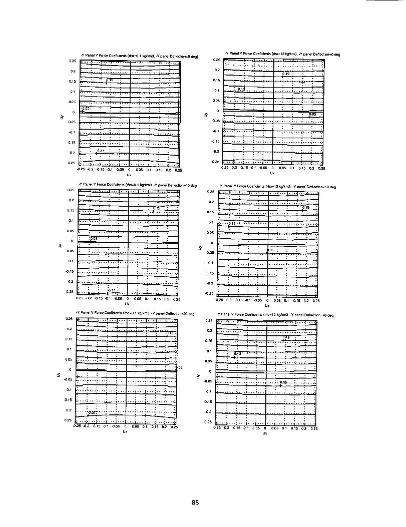
0.25
0.2
0,15
01
0.05
0
_.05
-0,1
-0.15
-02
-0.25
0.15
0.1
0.05
0
-0.05
-0_1
-0.15
-0.2
•0 .25
-Y Panel Y Force Coeficients (rho=0.1 kg/km3, -Y panel Deflection=0 deg]
:--.?...!..,!...! ....... :...!..._...- ....-- , ol_J t i 1 •
:- . . • . : ,
.. . . ...I. . . ', . . . ', . o . ; . . . , . . . i . . . , . . . .: .... . ....
..... | | . __• 0.03 -
,: - ; ; : - : : :
;: : " ' ' ' • : ... .... :..l-....}...- ....... ;....-...: .... -...-
L_ " _°:,._!...i ....... i...L• : " _. . . : ; . : . .
-0.25 -0.2 _,15 -0.1 -0.05 0 0.05 0.1 0.15 0.2 0,25
Ux
-Y Panel Y Force Coeficients (rho=0.1 kg/km3, -Y panel Deflection=10 deg
025 .#-_..L v v i_...i,.., j ....... i... !.,..,,,,,,,.- _
• . . ; ±
02 ............ • : " ..'..-..L
..-'::..L..._...;..., .................
_.!....!...; .._ ...... ;..,,:....: .... :....
...... ..... ,.--;---I_ ...... '---,[.--_-.._ .....
• t
:O0:Z: : I : ; : . .
: :, : - ....... :....:....;...;,.. ,... ;... ;....:....." .... .,_ - . , ; : : ; . "----.
......... 91 .................................
: : :.0.11 : .....
-0.25 -0.2 -0.15 -0.1 -0.05 0.05 0,1 0.15 0,2 0.25
Ux
-Y Pane{ Y Force Coeflc_nts (the=0.1 k_/km3, -Y pane{ Defk_ct_on=20 de{{
0.25
0.2
0.15
0.1
0.05
0
-0.05
-0.1
-0.15
-0.2
_.._.. ?....!...!........ :...;..._...;...
,2.... :....:....;...;...
...i.,,(,.,_..._..,_
• *T'''t ..... fr ....
.... ,
";'";'"_ .... :.... : .o3
: : : : : : : , :
:_!"'!'"i"i" i!" i "'<, .... !'"'_:
•025 ; .... -" " • "," " • ' | • ' " I ...... t'" • I' '" •:.'''': .... '
•0.25 -0.2 -0.15 -0.1 -0.05 0 0.05 0.1 0.15 0.2 0.25
Ux
-Y Panel Y Force Coeficients (d'm=12 kg/km3. -Y panel Deflection=0 deg
0.25i:::/:.... ;::'.;:,::i::'.i:::i:::i...-...._ ....
02 :.._. ;--!:,--i ........_;¥i---: ;0.15
Ol :-.-:l °;_ . ; .... ;...; ........... ,..• . , : : : : ; ; ,
-005 ...._....._. ,.. .............. ;.--;---.:..-.: .....
-- - ! ! • • • r0
• • • ; ; . • 0,O5: ; . ,_; .
--_ .... :, .................................-0.05
..... : : • . ,-0.1 ,....:..." ;...; ....... _...:.....:...; .... .
•0.15 _,,, " .,:,...:-.,.; ...... ;...,....:,,,.: .... :• : ; : : : ........... , o .
•0.2 ......... i .............
: : : : : : : : : :,, • | | i-025:....:....,...i...,......i...;..._..._...;
-0,25 -0.2 -0.15 _).f .0.05 0 0.05 0,1 0.15 0.2 0.25
Ux
-Y Panel Y Force Coerlcients (rho=12 kg/km3, -Y panel Deflection=tO deg
0.25 ,.... .....;,...i...t ...... {'"I''": ........" l - - • i i --
o._........... :...: ...."_'"!"'!"o:_"_[ --
0.15 w .... ,...,...,.......4...,...,...,...e .... -
0.1 _. • , ._.13.._ ...'... ! ...... ;-..:--.; .... "--..
0.05 _.... ..... '.....1..._...,.._1....;-_._.... ' .... .
0 ........ : "
..... _,.05-0.05 ..... •
: : : : • : : : : ,.,.... ;..•,,•,.!..._ ...... ,....,.. • ,,.... •....• ' : ; ; , - ....
_...;..., ..........,..._
: : : : : : : :
-0.25 -0.2 -0.15 .0.1 _.05 0 0.05 0.1 0.15 0.2 0.25
UX
-Y Pe,nei Y Force Coeficmnts (d-,o=12 kg/_rn3, -Y pane_ Oaflechon='20 de 9
'.... '-...:,..._---i ....... I-_,< ...•' ...' .... '
............. • ..." ....... : ..................• • • ' : : u:19 •
...... • ...:.,: ....... :.l: .:...J_.
-0.1
-0.15
-0.2
-0.25
0.25
0.2
O.f5
0.1
0.05
0
_ : . .
,'"'""OA_":"; -','_ : I1 : : :-...:...;.,.;...; ....
•0.05 ..... :....;...1...1...,'. ! !
-0.1
-0.15
-0.2
-0.25
-0.25 -0.2 -0.15 -0.1 -0.05
: : : : :. .i... ; .... o .... , .....
: : : ;... ;...,:...,: .... : ....
• .. ,. _,0_... _....: .... :,
±--!----;...;--.i ...... ;...;...; ....:.....
:_.L...'...:.._-- ...... 3...2...2...2...-": : : : : : : ; :
v..... ."• •":'" " 'l •- "| "''_ • "• l' •• I" • •":"• • "1.... ;'
0.05 0.1 0.15 0.2 0.25
Ux
85

025
02
O15
O1
0.05
0
-005
-01
-0.15
-Y Panel Y Force Coef_ienfs (rho=72 kg/1(m3. -Y panel De_sct_n=O deg
..... 1
._......,:...;...:..._...:...,...,; ...... ..:LJ_ • • * 019 • , • • •
;:.... :,,,,:,..:'..; ....... .;...;...; .... , .... .
• ., . . . ....
__" . ,.,....;...;...,...,..,;..._ .... ". .
::.... ;.,.,:J..;._ ,_. .....; ' . . .
.... 0.05 .....• '1 ' " ' ' --
_....;....;...; .......... ;....:.. • .: .... : .... .• . "_ : : ; [ _ . .
-o2 :i "_.,.;._..'.. :. = ..:_....'._.£__._
-0.25-0.2 0.15-0.1 -0,05 0.05 01 0_16 02 0.25
Ux
015
01
005
O
-0.05
-0.1
-0,15
-02
-025
-0.25 -0.2 -0.15 -0,1 -0.05
-Y Panel Y Force Coefictents (rho=120 kg._rn3. -y panel Deflection=0 delp
0.25 --'=,,'_-'''!"''1 ..... I'''('''_'', ="'_
;.._: : : : : : : : 30.2 ..... :, ....... " ........... :..,:: ...... :. .....
.;-.-i.... ;.,.;..,i ...... ;...;,..._ .... i.... :
• .'-':-';-;_--_"_'_'"..... o ....
..... o . o • .
..... : : : - ._
,.... :....;....,..., ..... _...,....: .... : .... :.
.,__ : __ . - o os .
....... .= . : .
0.0S 0.1 0,15 0.2 0.25
UX
025
02
015
01
005
0
-0,05
-01
-0.15
-Y Panel Y Force Coeficients ho=72 kg]km3. -Y panel Deflation= I0 deg
_.--...,....$ , . . i , . . ! . . ,':-,,_-_. i....b . , .I .... , ......
r'[; ; I • :': : ....
i
.-'T ._ ....... ,; ....... : ....... , "- .... "
: : , : .....
• " " 0._7 . " ....
:',1.; ..... ;...,;....: .... : .... ".
'-_ : • : :.,.,.,,,...,°.,,,...
• . . . ;
7,...;.,.-',- ;, :
: : ! . .
: • : :___"
• ..:...;.,, ; .... : .... :
=, ....
7o_. ! -- .... i...-
-02 ....' -,-,.,. ........... . ........... :" .........
-o.25_.... , _, , I....... , .- ._.- ._..... ;.... _.-0.25 -0,2 -0.15 -0.I -0.05 0.05 0.1 016 0,2 0,25
Ux
025
02
015
0.1
0.05
0
-0.05
-01
-015
-0.2
-025
-0,25 -0.2 -0.15 -0.1 -0.05
-Y Panel Y Force Coeficients (rho=72 kg._m3. -Y panel Deflectlon=20 deg
_.. : ; .... . .__:.... :.,.,'-,.,;,,,;,, ._ ....... ;. ........ ; ......
• , , ; ; ; ; _"
,...........:-...!...,.o_.... :,.-...-:-... .... :;.... ;.... ;,. ,,,,,.. : ....... :.,.;..,,; .... : .... .
• , , : : ; . .
•,, :: : : : ;om : : :. : :." . . . : : : : :
17 : i ? "' : _,r.'- . ........
-- - - v ! i i -
:.... .:...:..._...., ...... .....,.......... .... .......
,, ) : ; : : : : , ;
;.... :- ,,,; ,- ,; • ,- ; • -, ," • ;''";" • ":- -o _' • ":
:....'..,:,..'...: ....... :.,..:...;,,.- .... -
...... . • • •
;....; ; .i...i ...... i...i...,: ....;....;0.05 0,1 0 15 02 0.25
Ux
-Y Panel Y Fome Coeficients (rho=120 kg/km3. -Y panel Deflection=10 deg
0.25 Z=--,-I----'- "-I---I ....... I,--1"-'_ .... ;'''_',
: : : " : ; {)29: :
02 ..... ;...; ....................... t..._,,.._. . : : : : : ; , .
• . , . . , .....
.'-- : ; ..... :005 •.... _ ..._---_---*- -. ='--_--'_--'_ .... , .... ..
1 " " _ -
0
: : : : : : : : : :
l 1 • _: * • i-005 * .... . • ..,,,.,..o ....i.., _.., o,. ,*..,_ ......
• . ." ! ! : _ '. --
-0.1 .'.... ", • • ,", * *._ • ,, Z ...... I,,,;,.,_" .... ', -,.',
: : : : : : : : : .']
-02 ................. " - - • . • - - " ........... - .....
.... : :r-°;: ,. .025 ;.... ;-'-;-.-i,--t ..... _'-'_--'_ .... ;.... ;,
02_-0_ 0_ 01 00_ 00_01 01_o_ 025Ux
-Y Panel Y Force Coeficients (rho=120 k0/km3, -Y panel Deflection=20 deg
- _ i i i . . . ._: : : ' -"02 _":'"r'"'"'" ...... :'":'"v'":'"':
015 ..... - ............... ...., ........... ._D.33, ..
01 ¢.... ;..;_..._.......,..._....... r .... • .... ".
0.05 : ...__.;...1_. 17 :_r'" " " "
,_-- : : : ......
o ._, .... *l
.005 :-- -.,...,,:..._..._ ..? .._.. ; .... : .... _.
-0.I .:.... ";,..,_,.-: ,*. :,, • I, • .I... _...,; .... , .... :_
:__ - ; : : : ; ; : ;
-015 ;..... :,,,.;-,.;,,,; ..... ;...;....: .... :''":::5_.,
.. . o . . , ......-o,2 ..................... • .....................
-0.25 l .... i''"l'"i'"l'"l "'" I'""'": .... ; .... ;'
-0.25 -0_2 -0.15 -0,1 -005 0,05 0.1 0J5 0.2 0.25
Ux
=
86
I 1I-

0.25
0.2
0.15
0.1
0.05
0
-0.05
-0.1
=0.15
-0.2
-0.25
-y
_.-;.-.;...i ...... i... i... ;..._.,_...-0,25 -0.2 -0.15 -0.1 -0.05 0 0.05 0.1 0.15 0.2 0.25
UX
Panel X-Moment Coeficients (rho=0.1 kg_m3, -Y panel Deflection=O deg)
0.25
0.2
0.15
0.1
0.05
0
-0.05
-01
-0.15
-0,2
-0.25
-Y Panel X-Moment Coaficients (rho=0.1 kg/km3, -Y panel Deflection=lO deg
•
: __---'_ .
-0.25 -0.2 -0.15 -0.1 -0.05 0 0.05 0.1 0.15 0.2 0.25
UX
0,25
0.2
0.15
0.1
0.05
0
--005
-0.1
-0.15
-0.2
-0.25
.0.25 .0.2 .0,15 -0.1 -0.05
-Y Panel X-Moment Coeficients (rho=O.l k_km3, -Y panel Deflection=20 deg
0.14
0.05 0.1 0.'15 0.2 0._'5
Ux
0.25
0.2
0.15
0.1
0.05
0
.0,05
.0,1
-0.15
-0.2
-0.25
-Y Panel X-Moment Coeficients (rho= 12 kg/km3, -Y panel Deflection=O dog
•1,: :__'-- - .. - -t • • • I ...... ". - -
-0.25 -0.2 -0.15 -0.1 -0.05 0 0,05 0.1 0.15 0.2 0.25
UX
0.25
0.2
0.15
0.1
0.05
0
-0,05
-0,1
-0.15
-0.2
-0.25
ºY Panel X-Moment Coeficients (rho=12 kg/km3, -Y panel Deflection= 10 deg
_-_
_..;...i ..... i...i..._-0.25 -0.2 -0,15 -0.1 -0.05 0.05 0.1 0.15 0.2 0.25
Ux
0.25
0.2
0_15
0.1
0.05
0
-0.05
-0.1
-0,15
-0.2
.0.25
ºY Pane_ X-Moment Coeficients (rho=t2 kg/km3, -Y panel Deflection=20 deg
..... 1.18
: :_
_; .......
,[.... ;...;...;...;...-0.25 -0.2 -0.15 -0.1 -0.05
"';"';''": .... i .... "
.._..z...-.--• . o ,
•.i.--;-.-,[ .... _.... :0.05 0.t 0.15 0.2 0.25
Ux
87

0,25
02
0.15
01
0,05
0
*0.05
-0.1
-0.15
-0.2
-0+25
0.25
02
015
01
0,05
0
-Y Panel X-Moment Coeficients (rho=72 kg/km3, -Y panel DeflecUon=0 deg
...... , , . °
• : : : .
-0,2_5 -0.2 -015 -0.1 -0.05 0.05 0.1 0.15 0.2 025
Ux
-Y Panel X-Moment Coef;c]ents (rho=-72 kg/km3, -Y paner Deflect_n=10 deg
: - : - ; ; : - . :
.... • .......;...1... ..._...1..._ .... : .... :
-0.05 _
-01 _;-..
-0.15
-02
-025 _ - _ • • • I • ' " I, . - .,,
-0.25 -0.2 -0.15 -01 -0.05
Ux
.. ;.._
v,.. _ ,
0.05 0.1 0,I5 0.2 025
0.25
02
0t5
01
0.05
o
-0 05
-01
_15
-02
-025
-O,2S
-Y Pane_ X-Moment Codicients I .ho=72 kg/km3, -Y panel Deflection=20 deg
.r..- -,_.•-._-.. _-, •I ..... t--.{ .... :--" ":.... "
_-.._' ' " -o_'e :_._,_.--.i....:...:..._.............+...........:.....
,,,-,i,,,;
• . . ; -
2'i : ; +".... :
-.i,-,l_
.._...: .......:...:..._
• . . : -. , . J _ i ....
• • .1...:.,.: ....... :....'....'..." .... :
.... ;-..;...;..-; ..... i-.. i...,_...-..._-0.2 -O15-0.1 -0.05 0 0.05 O1 0.15 0.2 0.2S
Ux
-Y Panel X-Moment Coeficients (rho=120 k:g/km3, -Y panel Deflection=0 deg
0.25 { .... _''''."'''''''''''l "'''''''''''_ .... :''''.'_
02 _,_
0.15
005 ......... , ,:;
.o.o .......;., ,,,, ..., .., ,,,. ............. ; .... • .... ,
-o15 .:.... _,.._-..,..., ....
.02_0.25
o.25UX
-Y Panel X-Moment Coeflclents (rho=120 ko/km3, -Y panel Deflectlon=10 (:leg
0.25 ..J.. • ,_. • . ,_. • • * . .,---.4,.,-,"e'T'_..,.. ..... ,_ .: .... ',
020.15 _..._..._..-. ....... I...,...,...- .... ".... ",
oo__..; ...... ;-_
o _ j . : . .
-0.05 * .... ,...,...,...,...a...,...,..., ..........
-01_'...'..." ....:"
Q2.+_ : : ,'o10:.2.....
-o25_.!...!:i i ! ! !...!._-0.25 -0.2 -0.15 -0,1 -0.05 0.05 0.1 0,15 0.2 0.25
Ux
-Y Panel X-Moment Coeficients (rho=120 kg/km3, -Y panel Deflection=20 dog
0.25 __- - - I - • ' 1- • - ': .... : .... :'
0.2 _,-,. ............... i,,-, .................
: : : : :
o.15 _ ! ! " " - .........
0.1 ; ,; ", • • ; • • • ; ...... " "_
: ; ; : - , : : : : -
o.o ...,._.,.._:....o
-0.05
-01
-0,15
-0.2
..0,25 ,:,.... ,"''':''''l'''l''
-0.25 -0.2 -0.I5 -0.1 -0.05
_'- . .' ; ,
i_..:...-:..-.;..-i......."---'-.-"....:....:,........ -0.12' •.... _.,._ ...I.,.;-- .,- • - :--- ,- .--:;,. ,.: .... 1,
- : .i.._i_..!.......!...£...2...'...-
..... I " " ' ! • , • _..... : .... :'
0_05 0.I 0,15 0.2 0.25
Ux
88
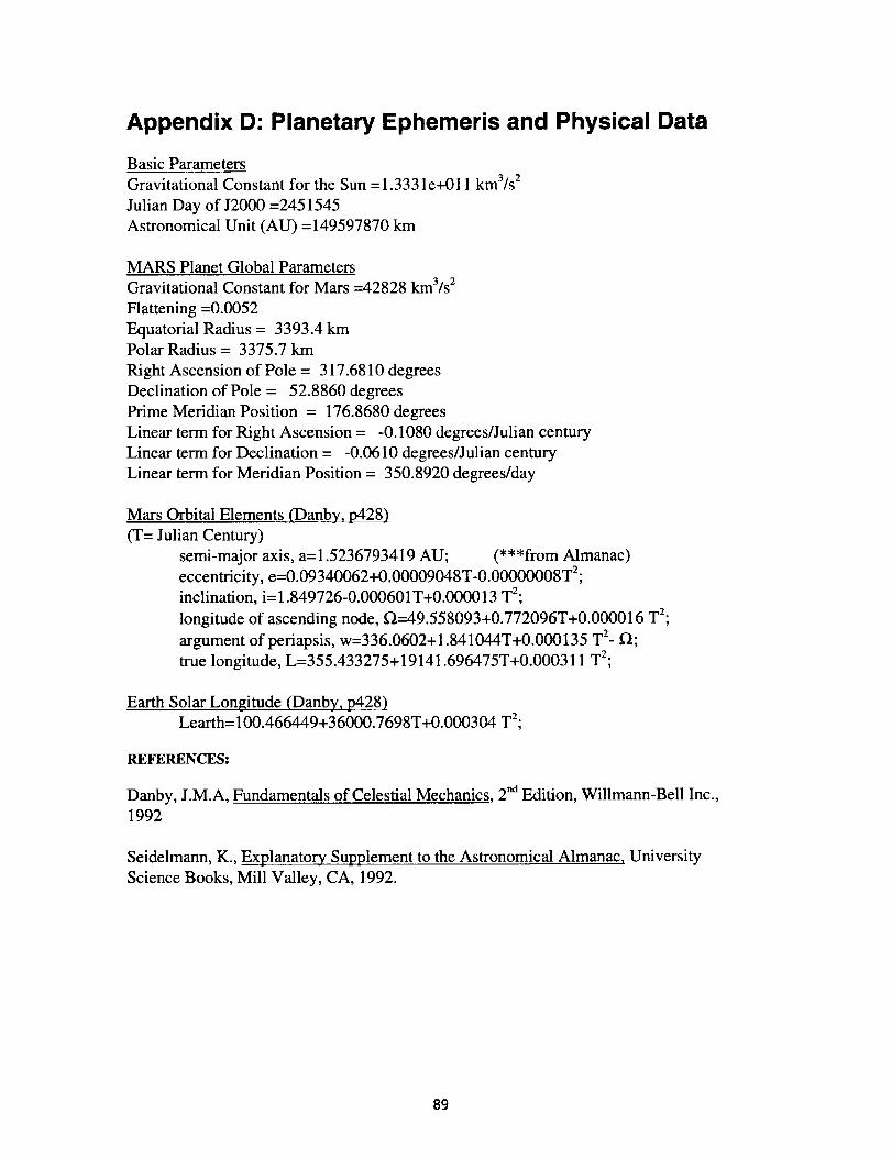
Appendix D: Planetary Ephemeris and Physical Data
Basic Parameters
Gravitational Constant for the Sun =1.3331e+011 km3/s 2
Julian Day of J2000 =2451545
Astronomical Unit (AU) =149597870 km
MARS Planet Global Parameters
Gravitational Constant for Mars --42828 km3/s 2
Flattening --0.0052
Equatorial Radius = 3393.4 km
Polar Radius = 3375.7 km
Right Ascension of Pole = 317.6810 degrees
Declination of Pole = 52.8860 degrees
Prime Meridian Position = 176.8680 degrees
Linear term for Right Ascension = -0.1080 degrees/Julian century
Linear term for Declination = -0.0610 degrees/Julian century
Linear term for Meridian Position = 350.8920 degrees/day
Mars Orbital Elements (Danby, p428)
(T= Julian Century)
semi-major axis, a=1.5236793419 AU; (***from Almanac)
eccentricity, e=0.09340062+0.00009048T-0.00000008T2;
inclination, i=1.849726-0.000601T+0.000013 T2;
longitude of ascending node, f_=49.558093+0.772096T+0.000016 T2;
argument of periapsis, w=336.0602+ 1.841044T+0.000135 T 2- fl;
true longitude, L=355.433275+ 19141.696475T+0.000311 T2;
Earth Solar Longitude (Danby, p428)Learth= 100.466449+36000.7698T+0.000304 T2;
REFERENCES:
Danby, J.M.A, Fundamentals of Celestial Mechanics, 2 noEdition, Willmann-BeU Inc.,
1992
Seidelmann, K., Explanatory Supplement to the Astronomical Almanac, University
Science Books, Mill Valley, CA, 1992.
89

Appendix E: MGS Physical Properties
S/C Mass (kg)S/C CG (m)Ixx S/C about S/C CG (kg-m2)
SAM Mass (kg)SAM Azimuth (deg)SAM CG (m)Ixx SAM about SAM CG (kg-m2)
Distance from S/C CG to SAM CG
Location of Failure Line (m)Distance from Failure to SAM CG
BUS+SAP MassBUS+SAP CG
Distance from B+S CG to SAM CG
Ixx SAM about B+S CGDistance from B+S CG to S/C CG
Ixx BUS+SAP about B+S CG
-3E-04
-0.006
Mid Yoke Failure
(D.
Shaffer)763.2
-0.0011 1.3551043
39.3433.4
-2.386 2.0764.805
0.0057 2.3849 -0.715
( 2.4898 )
0.0381
1E-05
-0.9045 1.0861.7791
723.860.1285 1.31614
0.006 2.5145 -0.7539( 2.6251 )
335.90.0003
(
0.1296 -0.0389
0.1353 )693.84
-3E-04
-0.023
Hinge LineFailure
763.2-0001 1.3551043
27.89633.4
-2.789 2.338847.09
0.0223 2.7883 -0.984
( 2.9569 )
0.0381 -1.313 1.3551.7752
735.30.0005 0.1047 1.3177
0.0231 2.8941 -1.021( 3.069 )
309.840.0008 0.1058 -0.037
( 0.1122 )723.91
from B+S CG to Failure) I 0.0381ABS(Dist.Position of Z accelerometer -0.44
a
1.033-0.38
b a b
0.23014 I 0.0376 1.4177 0.03732.05 / -0.44 -0.38 2.05
90
HI_| I-
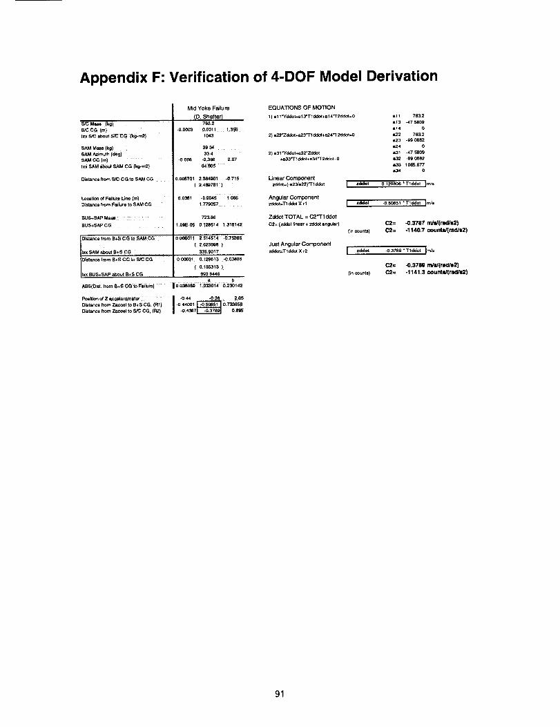
Appendix F: Verification of 4-DOF Model Derivation
S/C CG [m)
tx:< S/C aboul _ CG (kg-m2)
BAM Mae,s [kg]
SAM Azimuth (deg]
SAM CG (m]
txx SAM about SAM CG _kg-m2)
Dtstarce from SJC CG 1o SAM CG
Location of Faiture Line (m'J
D_stance from Failure to SAM CG
BUS+SAP Mass
BUS+SAP CG
DIstance from B+_ CG lo _,AM CG 0006011 2.514514 -O.7_186{ 2._25095 ]
lxx SAM about B+S CG 336.9017
Dista_cefromB+SCGtoS/CCG 000031 0.129613 -0.03886[ 0._35313 )
Ilxx BUS+SAP about B+S CG 5g3.8446• D
ABS(Dist. from B+_ C_ to FaikJm} O.03808g I 0S_1014 0.230142
Pos_ion of Z tcceleromefer | *044 -0.36 2.05
I-0.44001Distanco from Zaceel to B+S CG. (R1) [].7338.._
Distance from Zaccef to S/C CG, (R2} -0.4307 069=3
Mid Yoke Failure EQUATIONS OF MOTION
ID. Shafter) 1) el l"Yddot+a13"T1ddot+a14"T2ddot=07832
-0.0003 -0.001 _ 1.35_
1043 2) e22"Zddot +¢23 _'1"1 ddot ÷ e24"T2ddot =0
3_34
33.4 2) e.31"Yddot _*e32* Zddot
-0.OO6 -2.386 2.07 .t4_3*T1 ddot+ e.34"T2ddot =0
648O5
0.005"701 2.384901 -0.715 Linear Component
( 2.41_761 ) zdd_=(.e23/==22)_'1ddot
0.038_ -0.g045 1.00S Angular Component
1 .T_9_'7 zddot=Tlddot X r_
723.66 Zddot TOTAL = C2"T'1 ddot
109E-05 0,128514 1316142 C2=(zddotffnear+zddotengular)
Just Angular Component
zddot=Tlddot X r2
I zddot
B11 763.2
S13 -47.580g
a14 0
It22 763.2
=23 -9g.0682
a24 0
_1 °475809
a32 -99 0662
a33 1065677
a34 0
0.129606 *Tlddot ]m/s
I zddot _0.50e51 " Tlddot ]rrVs
C2= -0.3787 m/#(rad/a2)
(in counts) C2= -1140.7 counts/(rad/s2)
zddot
(in counts)
-03789 "Tlddot IrrVs
C2= -0.3789 mhd(rad/s2)
C2= -1141,3 counts/(rad/s2)
91

REPORT DOCUMENTATION PAGE o__,=
Public reporting burden for this c_lection of information ts estimated to average 1 hour per response, including the _.me for revlewlnglnstructions, searching sxis_g data sources,gathe.dng an_:lmalnta...inin¢J _ ..dataneed_.., _ completing and.reV.,pwl,ng the colle@n of I_ormation. Send comments .r_a_tng this burden estimate or any other aspect of thiscollection OTtnrorrnadon, lnouoing suggeslions ror reoucing this Duroen, to Washington Heaoquaners Ser,Aces, Directorate TOtlnTorrnationuperations and Reports, t 215 JeffersonDavis Highway, Suite 1204, Arlington, VA 22202-4302, and to the Office of Management and Budget, Paperwork Reduction Pro act (0704-0188), Washington, DC 20503.
1. AGENCY USE ONLY (Leave blank) 2. REPORT DATE 3. REPORT TYPE AND DATES COVERED
October 1998 Contractor Report4. TITLE AND SUBTITLE 5. FUNDING NUMBERS
Operational Data Reduction Procedure for Determining Density and Vertical
Structure of the Martian Upper Atmosphere From Mars Global Surveyor NCC1-104Accelerometer Measurements
6.AUTHOR(S) 865-10-03-01George J. Cancro, Robert H. Tolson, and Gerald M. Keating
7. PERFORMINGORGANIZATIONNAME(S)ANDADDRESSEES)
The George Washington University
Joint Institute for Advancement of Flight Sciences
NASA Langley Research Center
Hampton, VA 23681-2199
9. SPONSORING/MONITORINGAGENCYNAME(S)ANDADDRESS(ES)
National Aeronautics and Space Administration
Langley Research Center
Hampton, VA 23681-2199
8. PERFORMING ORGANIZATIONREPORT NUMBER
10. SPONSORING/MONITORINGAGENCY REPORT NUMBER
NASA/CR- 1998-208721
11. SUPPLEMENTARY NOTES
The information submitted in this report was offered as a thesis by the first author in partial fulfillment of the
requirements for the Degree of Master of Science, The George Washington University, JIAFS.
Langley Technical Monitor: Robert Buchan12a. DISTRIBUTION/AVAILABILITY STATEMENT 1213. DISTRIBUTION CODE
Unclassified-Unlimited
Subject Category 91 Distribution: Nonstandard
Availability: NASA CASI (30I) 621-0390
13. ABSTRACT (Maximum 200 words)
The success of aerobraking by the Mars Global Surveyor (MGS) spacecraft was partly due to the analysis of MGSaccelerometer data. Accelerometer data was used to determine the effect of the atmosphere on each orbit, to characterizethe nature of the atmosphere, and to predict the atmosphere for future orbits. To interpret the accelerometer data, a datareduction procedure was developed to produce density estimations utilizing inputs from the spacecraft, the NavigationTeam, and pro-mission aerothermodynamic studies. This data reduction procedure was based on the calculation ofaerodynamic forces from the accelerometer data by considering acceleration due to gravity gradient, solar pressure,angular motion of the MGS, instrument bias, thruster activity, and a vibration component due to the motion of thedamaged solar array. Methods were developed to calculate all of the acceleration components including a 4 degree offreedom dynamics model used to gain a greater understanding of the damaged solar array. The total error inherent to thedata reduction procedure was calculated as a function of altitude and density considering contributions from ephemeriserrors, errors in force coefficient, and instrument errors due to bias and digitization. Comparing the results from thisprocedure to the data of other MGS Teams has demonstrated that this procedure can quickly and accurately describe thedensity and vertical structure of the Martian upper atmosphere.
14. SUBJECT TERMS
Mars Global Surveyor mission; Space flight; Mechanics
17. SECURITY CLASSIRCATICNOF REPORT
Unclassified
N S N "754_0 i"-"_.8'0- 5500
ii
18. SECURITY CLaSSIRCATIONOF THIS PAGE
Unclassified
19. SECURITY CLASSIFICATIONOF ABSTRACT
Unclassified
15. NUMBER OF PAGES
10616. PRICE CODE
A0620. UMITATION
OF ABSTRACT
Standard Form 298 (Rev. 2-89)Prescrfoed by ANSI Std. Z-39-18
92
-:l| I-


