On the Nature of Capital Adjustment Costs∗
Russell W. Cooper
Department of Economics, University of Texas at Austin,
BRB 1.116, Austin, Texas 78712, USA
John C. Haltiwanger
Department of Economics, University of Maryland,
College Park, Md. 20742, USA
November 22, 2005
Abstract
This paper studies the nature of capital adjustment at the plant level. We usean indirect inference procedure to estimate the structural parameters of a rich speci-fication of capital adjustment costs. In effect, the parameters are optimally chosen toreproduce a set of moments that capture the nonlinear relationship between investmentand profitability found in plant-level data. Our findings indicate that a model whichmixes both convex and non-convex adjustment costs fits the data best.
∗The authors thank the National Science Foundation for financial support. Andrew Figura, Chad Syver-sons and Jon Willis provided excellent research assistance in this project. We are grateful to Shutao Cao forhis comments on the final versions of this paper. Comments and suggestions from referees and the editorof this journal are gratefully acknowledged. We are grateful to Andrew Abel, Victor Aguirregabiria, Ri-cardo Caballero, Fabio Canova, V.V. Chari, Jan Eberly, Simon Gilchrist, George Hall, Adam Jaffe, PatrickKehoe, John Leahy, David Runkle and Jon Willis for helpful discussions in the preparation of this paper.Helpful comments from seminar participants at Boston University, Brandeis, CenTER, Columbia University,the 1998 Winter Econometric Society Meeting, the University of Bergamo and IFS Workshop on AppliedEconomics, the University of Texas at Austin, UQAM, Federal Reserve Bank of Cleveland, Federal ReserveBank of Minneapolis, Federal Reserve Bank of New York, Pennsylvania State University, Wharton School,McMaster University, Pompeu Fabra, Yale and the NBER Summer Institute are greatly appreciated. Thedata used in this paper were collected under the provisions of Title 13 US Code and are available for use atthe Center for Economic Studies (CES) at the U.S. Bureau of the Census. The research in this paper wasconducted by the authors as Research Associates of CES. The views expressed here do not represent thoseof the U.S. Census Bureau.
1
1 Motivation
The goal of this paper is to understand the nature of capital adjustment costs. This topic
is central to the understanding of investment, one of the most important and volatile com-
ponents of aggregate activity. Moreover, understanding of the nature of adjustment costs is
vital for the evaluation of policies, such as tax credits, that attempt to influence investment
and thus aggregate activity. Despite the obvious importance of investment to macroeco-
nomics, it remains an enigma.
Costs of adjusting the stock of capital reflect a variety of interrelated factors that are
difficult to measure directly or precisely so that the study of capital adjustment costs has
been largely indirect through studying the dynamics of investment itself. Changing the level
of capital services at a business generates disruption costs during installation of any new
or replacement capital and costly learning must be incurred as the structure of production
may have been changed. Installing new equipment or structures often involves delivery lags
and time to install and/or build. The irreversibility of many projects caused by a lack of
secondary markets for capital goods acts as another form of adjustment cost.
Some industry case studies (e.g., Holt et al. [1960], Peck [1974], Ito et al. [1999]) provide
a detailed characterization of the nature of the adjustment costs for specific technologies. A
reading of these industry case studies suggest that there are indeed many different facets of
adjustment costs and that, in terms of modeling these adjustment costs, both convex and
non-convex elements are likely to be present.1
Despite this perspective from the industry case studies, the workhorse model of the
investment literature has been a standard neoclassical model with convex costs (often ap-
proximated to be quadratic) of adjustment. This model has not performed that well even at
the aggregate level (see Caballero [1999]) but the recent development of longitudinal estab-
lishment databases has raised even more questions about the standard convex cost model.
An alternative approach, highlighted in the work of Doms-Dunne [1994], Cooper, Halti-
wanger and Power [1999], Abel-Eberly [1994, 1996], and Caballero, Engel and Haltiwanger
1Holt et. al. [1960] found a quadratic specification of adjustment costs to be a good approximation ofhiring and layoff costs, overtime costs, inventory costs and machine setup costs in selected manufacturingindustries. These components of adjustment costs for changing the level of production are relevant herebut are by no means the only relevant costs. In terms of changes in the level of capital services, Peck[1974] studies investment in turbogenerator sets for a panel of 15 electric utility firms and found that “Theinvestments in turbogenerator sets undertaken by any firm took place at discrete and often widely dispersedpoints of time.”In their study of investment in large scale computer systems, Ito, Bresnahan and Greenstein[1999] also find evidence of lumpy investment. Their analysis of the costs of adjusting the stock of computercapital include items which they term “... intangible organization capital such as production knowledge andtacit work routines.” Hamermesh and Pfann [1996] also provide a detailed review of convex adjustment costmodels and numerous references to the motivation and results of that lengthy literature.
2
[1995], argues that non-convexities and irreversibilities play a central role in the investment
process. The primary basis for this view, reviewed in detail below, is plant-level evidence
of a nonlinear relationship between investment and measures of fundamentals, including
investment bursts (spikes) as well as periods of inaction.
One limitation of this recent empirical literature is that it has focused primarily on
reduced form implications of non-convex vs. convex models. The results that emerge reject
the reduced form implications of a pure convex model and are consistent with the presence of
non-convexities. The reduced form nature of the results have left us with several important,
unresolved questions: what is the nature of the capital adjustment process at the micro level?
Does the micro evidence support the presence of both convex and non-convex components
of adjustment costs as might be expected based upon the limited number of industry case
studies? More specifically, what are the structural estimates of the convex and non-convex
components of adjustment costs that are consistent with the micro evidence? Finally, what
are the aggregate and policy implications of the estimated investment model?
To address these questions, this paper considers a rich model of capital adjustment which
nests alternative specifications. To do so, we specify a dynamic optimization problem at the
plant level which incorporates both convex and non-convex costs of adjustment as well as
irreversible investment. The model’s implications are matched with plant-level observations
from the Longitudinal Research Database (LRD) as part of a minimum distance estimation
routine. We recover structural estimates of adjustment costs.
There are a couple of key features of the data which guide the estimation: the frequency
of large bursts of investment, the positive correlation between investment and the marginal
profitability of capital and the relatively low serial correlation of investment. All of these
moments are computed at the plant level. These moments are chosen partly due to their
prominence in the literature and partly due to their informativeness about the underlying
structural parameters which we estimate.
Our results can be summarized by referring to extreme models.2 In the absence of
adjustment costs, investment is excessively responsive to shocks and is negatively serially
correlated. From this perspective, the role of adjustment costs is to temper the response of
investment to fundamentals and to create the slightly positive serial correlation of investment
observed at the plant level. The convex cost of adjustment model is not sufficiently sensitive
to shocks and creates excessively significant positive serial correlation of investment rates.
In particular, a model with convex costs alone cannot produce the bursts of investment and
inaction observed in the data. Thus richer models of adjustment are needed. Both the non-
convex and the irreversibility models are able to produce relationships between investment
2These comments pertain to the models studied in Section 3 and summarized in Tables 2 and 3. Asexplained below, these statements reflect not only the adjustment costs but also the driving processes.
3
and fundamentals which are much closer to the data. Both of these models imply inactivity
and investment bursts. Interestingly, irreversibility creates an asymmetry as well since the
loss from capital sales is more relevant when profitability shocks are below their mean.
From our estimation of a structural model of adjustment, a combination of non-
convex adjustment costs and irreversibility enables us to fit prominent features
of observed investment behavior at the plant-level. In particular, a model of
adjustment in which the non-convex costs entails disruption of the production
process fits the data best.
In terms of macroeconomic implications, the natural question is whether these non-
convexities ”matter” for aggregate investment. Our findings indicate that at the plant level,
the non-convexities identified in our estimation are important: a model with only convex
adjustment does poorly at the plant level. However, a model with only convex adjustment
costs fits the aggregate data created by our estimated model reasonably well though (as
reported independently by Cooper, Haltiwanger and Power [1999], hereafter CHP) the convex
models tend not to track investment well at turning points. Thus, we find that the non-
convexities are less important at the aggregate relative to the plant level. We relate this
finding to results reported by Caballero and Engel [1999] and Thomas [2002] in Section 5.
2 Facts
In this section we discuss our data set. We then present some moments from the data which
will guide the remainder of the analysis.
2.1 Data Set
Our data are a balanced panel from the Longitudinal Research Database (LRD)consisting of
approximately 7,000 large, manufacturing plants that were continually in operation between
1972 and 1988.3 This particular sample period and set of plants is drawn from the dataset
used by Caballero, Engel and Haltiwanger [1995], hereafter CEH. The unique feature of
this data relative to other studies that have used the LRD to measure investment is that
information on both gross expenditures and gross retirements (including sales of capital)
are available for these plants for these years (Census stopped collecting data on retirements
in the late 1980s in its Annual Survey of Manufactures which is why our sample ends in
1988). Incorporating retirements (and in turn sales of capital) is especially important in
3While the balanced panel enables us to avoid modeling the entry/exit process there is likely a selectionbias induced. Our use of the balanced panel is based on the difficult measurement issues for measuringreal capital stocks and in turn real capital expenditures and real capital retirements. The details of thismeasurement are described in Caballero, Engel and Haltiwanger [1995].
4
this exploration of adjustment costs and frictions in adjusting capital at the micro level.
Investigating the role of transactions costs and irreversibilities is quite difficult with the use
of expenditures data alone.
The use of the retirements data requires a somewhat modified definition of investment.
The definition of investment and capital accumulation follows that of CEH and satisfies:
It = EXPt −RETt (1)
Kt+1 = (1− δt)Kt + It (2)
where It is our investment measure, EXPt is real gross expenditures on capital equipment,
RETt is real gross retirements of capital equipment, Kt is our measure of the real capital
stock (generated via a perpetual inventory method at the plant level), and δt is the in-use
depreciation rate. This measurement specification differs from the usual one that uses only
gross expenditures data and the depreciation rate captures both in-use and retirements.
Following the methodology used in CEH, we use the data on expenditures and retirements
along with investment deflators and BEA depreciation rates to construct real measures of
these series and also an estimate of the in-use depreciation rate.4 In what follows, we focus
on the investment rate, It/Kt, which can be positive or negative.
2.2 Investment Moments
The histogram of investment rates that emerges from this measurement exercise are reported
in Figure 2.2. It is transparent that the investment rate distribution is non-normal having
a considerable mass around zero, fat tails, and is highly skewed to the right (standard
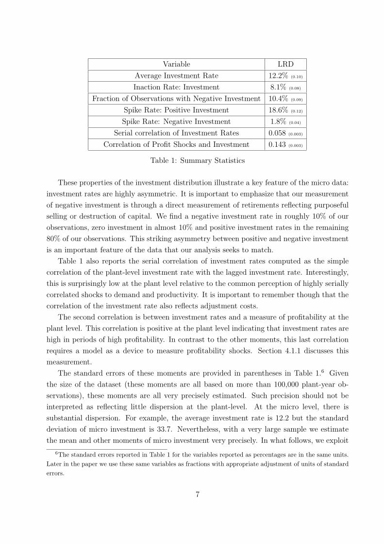
tests for non-normality yield strong evidence of skewness and kurtosis). Some of the main
features of the distribution (and its underlying components in terms of gross expenditures
and retirements) are summarized in Table 1.
First, note that about 8% of the (plant, year) observations entail an investment rate
near zero (investment rate less than 1% in absolute value). Of this inaction, about 6% of
the observations indicate gross expenditures less than 1% of the plant capital stock and the
4A relevant measurement point is that the retirement data are based upon sales/retirements of capitalwhich yield a change in the book value of capital. Using a FIFO structure and the history of investment andretirements, CEH develop a method to convert this to a real measure of retirements. The methodology yieldsa measure of the real changes in the plant-level capital stock induced by retirements. In what follows, it isimportant to note that this procedure does not already capture the difference between buying and sellingprices of capital that may influence the adjustment process. We recover that difference in our estimation.
5
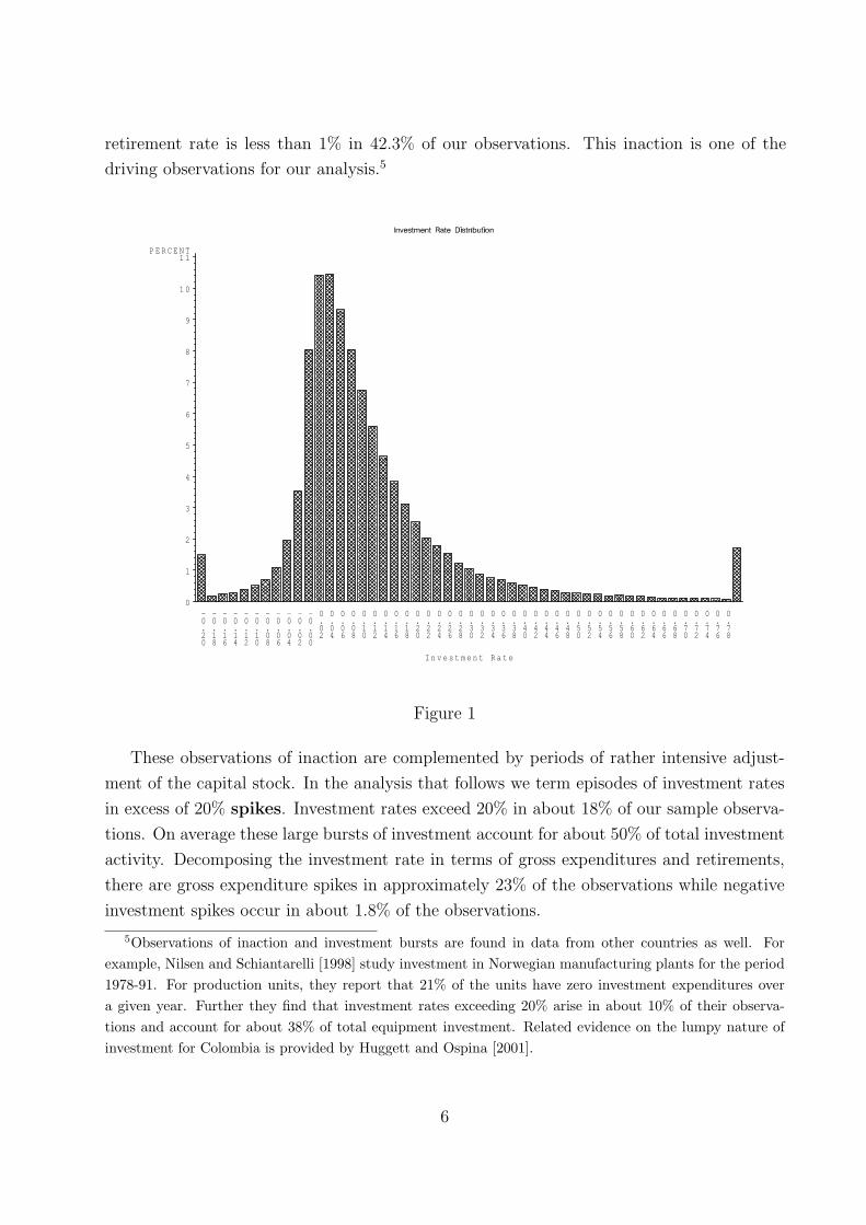
retirement rate is less than 1% in 42.3% of our observations. This inaction is one of the
driving observations for our analysis.5
P E R C E N T
0
1
2
3
4
5
6
7
8
9
1 0
1 1
I n v e s t m e n t R a t e
-0.20
-0.18
-0.16
-0.14
-0.12
-0.10
-0.08
-0.06
-0.04
-0.02
-0.00
0.02
0.04
0.06
0.08
0.10
0.12
0.14
0.16
0.18
0.20
0.22
0.24
0.26
0.28
0.30
0.32
0.34
0.36
0.38
0.40
0.42
0.44
0.46
0.48
0.50
0.52
0.54
0.56
0.58
0.60
0.62
0.64
0.66
0.68
0.70
0.72
0.74
0.76
0.78
Figure 1
These observations of inaction are complemented by periods of rather intensive adjust-
ment of the capital stock. In the analysis that follows we term episodes of investment rates
in excess of 20% spikes. Investment rates exceed 20% in about 18% of our sample observa-
tions. On average these large bursts of investment account for about 50% of total investment
activity. Decomposing the investment rate in terms of gross expenditures and retirements,
there are gross expenditure spikes in approximately 23% of the observations while negative
investment spikes occur in about 1.8% of the observations.
5Observations of inaction and investment bursts are found in data from other countries as well. Forexample, Nilsen and Schiantarelli [1998] study investment in Norwegian manufacturing plants for the period1978-91. For production units, they report that 21% of the units have zero investment expenditures overa given year. Further they find that investment rates exceeding 20% arise in about 10% of their observa-tions and account for about 38% of total equipment investment. Related evidence on the lumpy nature ofinvestment for Colombia is provided by Huggett and Ospina [2001].
6
Variable LRD
Average Investment Rate 12.2% (0.10)
Inaction Rate: Investment 8.1% (0.08)
Fraction of Observations with Negative Investment 10.4% (0.09)
Spike Rate: Positive Investment 18.6% (0.12)
Spike Rate: Negative Investment 1.8% (0.04)
Serial correlation of Investment Rates 0.058 (0.003)
Correlation of Profit Shocks and Investment 0.143 (0.003)
Table 1: Summary Statistics
These properties of the investment distribution illustrate a key feature of the micro data:
investment rates are highly asymmetric. It is important to emphasize that our measurement
of negative investment is through a direct measurement of retirements reflecting purposeful
selling or destruction of capital. We find a negative investment rate in roughly 10% of our
observations, zero investment in almost 10% and positive investment rates in the remaining
80% of our observations. This striking asymmetry between positive and negative investment
is an important feature of the data that our analysis seeks to match.
Table 1 also reports the serial correlation of investment rates computed as the simple
correlation of the plant-level investment rate with the lagged investment rate. Interestingly,
this is surprisingly low at the plant level relative to the common perception of highly serially
correlated shocks to demand and productivity. It is important to remember though that the
correlation of the investment rate also reflects adjustment costs.
The second correlation is between investment rates and a measure of profitability at the
plant level. This correlation is positive at the plant level indicating that investment rates are
high in periods of high profitability. In contrast to the other moments, this last correlation
requires a model as a device to measure profitability shocks. Section 4.1.1 discusses this
measurement.
The standard errors of these moments are provided in parentheses in Table 1.6 Given
the size of the dataset (these moments are all based on more than 100,000 plant-year ob-
servations), these moments are all very precisely estimated. Such precision should not be
interpreted as reflecting little dispersion at the plant-level. At the micro level, there is
substantial dispersion. For example, the average investment rate is 12.2 but the standard
deviation of micro investment is 33.7. Nevertheless, with a very large sample we estimate
the mean and other moments of micro investment very precisely. In what follows, we exploit
6The standard errors reported in Table 1 for the variables reported as percentages are in the same units.Later in the paper we use these same variables as fractions with appropriate adjustment of units of standarderrors.
7
the micro heterogeneity explicitly as we use the estimated dispersion of profit shocks from
the micro data.
We estimate adjustment cost parameters by using a simulated method of moments ap-
proach. This approach requires selecting moments to match. Theoretical and practical
considerations suggest that the moments should be relevant in identifying the adjustment
cost parameters and are also precisely estimated. We regard the four moments in Table 1 as
capturing key features of the behavior of investment at the micro level.
The first moment is the serial correlation in investment. It is well-established in the
adjustment cost literature (see, e.g., Caballero and Engel [2003] and CHP) that the serial
correlation of investment is sensitive to the structure of adjustment costs. The second mo-
ment is the correlation between investment and profit shocks as it reflects the covariance
structure between investment and the shocks to profits. This moment and the others we
match are quite sensitive to the adjustment cost parameters and in this sense satisfy the rel-
evance criterion. The other two moments capture key features of Figure 2.2 that have been
emphasized in the literature – namely that the investment distribution at the micro level
is very asymmetric and has a fat right tail. To capture these features, we use the positive
and negative spike rates in Table 1. Each of these four moments captures key features of
investment behavior at the micro level but the exact choice of moments is an open question.
In what follows, we use these four moments in our empirical analysis and then present some
analysis of robustness of our findings to the choice of alternative moments.
Before proceeding it is worth noting that one moment we choose not to match directly
is the fraction of observations with inaction. While Table 1 shows some range of inaction,
the more robust finding in Figure 2.2 and Table 1 is that the distribution of investment
is skewed and kurtotic with a fat right tail. Identifying inaction precisely at the micro
level is difficult because in practice there is substantial heterogeneity in capital assets with
associated heterogeneity in adjustment costs. For example, buying a specific tool gets lumped
into capital equipment expenditures in the same way as retooling the entire production line.
Explicitly analyzing the role of capital heterogeneity is beyond the scope of this paper but
we discuss this as an area of future research in the concluding remarks.
3 Models and Quantitative Implications
Our most general specification of the dynamic optimization problem at the plant-level is
assumed to have both components of convex and non-convex adjustment costs as well as
irreversibility. Formally, we consider variations of the following stationary dynamic pro-
gramming problem:
8
V (A,K) = maxI
Π(A,K)− C(I, A,K)− p(I)I + βEA′|AV (A′, K ′) ∀(A,K) (3)
where Π(A,K) represents the (reduced form) profits attained by a plant with capital K, a
profitability shock given by A, I is the level of investment and K ′ = K(1 − δ) + I. Here
unprimed variables are current values and primed variables refer to future values. In this
problem, the manager chooses the level of investment, denoted I, which becomes productive
with a one period lag. The costs of adjustment are given by C(I, A,K). This function is
general enough to have components of both convex and non-convex costs of adjustment.
Irreversibility is encompassed in the specification if the price of investment, p(I), depends
on whether there are capital purchases or sales.
Current profits, for given capital, are given by Π(A,K), where the variable inputs (L)
have been optimally chosen, a shock to profitability is indicated by A and K is the current
stock of capital. That is,
Π(A,K) = maxL
R(A, K, L)− Lw(L)
where R(A,K, L) denotes revenues given capital (K), variable inputs (L) and a shock to
revenues, denoted A. Here Lw(L) is total cost of variable inputs. Clearly this formulation
assumes there are no costs of adjusting labor. Once we specify a revenue function, we can use
this optimization problem to determine L and to derive the profit function Π(A,K), where
A reflects both the shocks to the revenue function and variations in costs of L. Throughout
the analysis, the plant level profit function is specified as
Π(A,K) = AKθ. (4)
This section of the paper provides an overview of the competing models of adjustment.
The parameterizations are summarized in Table 2, at the end of this section.7 For each, we
describe the associated dynamic programming problem and display some of the quantitative
predictions of the models in Table 3. At this stage these quantitative properties are meant
to facilitate an understanding of the competing models. Accordingly, the parameter values
are set to“reasonable” levels from the literature. The next section of the paper discusses
estimation of underlying parameters.
3.1 Common Elements of the Specification
For the following simulations, the aggregate and idiosyncratic shocks are represented by first-
order, Markov processes. Following Tauchen [1986], the set of aggregate and idiosyncratic
7In the estimation, determining the value of θ and the parameterization of the stochastic process for A isof course critical. The simulations that follow use the estimated values which are discussed in section 4.1.1.
9
profitability states as well as the transition matrices are chosen to reproduce the variance
and serial correlation of the profitability shocks inferred from our analysis of plant level
profitability. For the remaining parameters, we set the annual discount factor (β) at .95 and
the annual rate of depreciation at (δ) 6.9%. This depreciation rate is consistent with the one
used to create the capital stock series at the plant level less a retirement rate of 3.2%.
3.2 Convex Costs of Adjustment
The traditional investment model assumes that costs of adjustment are convex. Here we
adopt a quadratic cost specification and consider the following specification of the adjustment
function,
C(I, A,K) =γ
2(I/K)2K
where γ is a parameter. The first-order condition for the plant level optimization problem
relates the investment rate to the derivative of the value function with respect to capital and
the cost of capital, p. That is, the solution to (3) implies
i = (1/γ)[βEVk(A′, K ′)− p] (5)
where i is the investment rate, (I/K), and EVk is the expectation of the derivative of the
value function in the subsequent period. In practice, this derivative is not observable.
As suggested by (5), the investment rate reflects the difference between the expected
marginal value of capital, EVk(A′, K ′), and the cost of capital p. From this condition and
the one-period time to build assumption, investment responds to predictable variations in
profitability.
If profits are proportional to the capital stock, θ = 1, the model reduces to the familiar
“Q theory” of investment in which the value function is proportional to the stock of capital.
As in Hayashi [1982], the derivative of the value function can be inferred from the average
value of a firm, Vk(A,K) = V (A,K)/K.
In the special case of no adjustment costs, C(I, A,K) ≡ 0, from (3), the optimal capital
stock for the plant satisfies:
βEVk(A′, K ′) = p.
In the absence of adjustment costs, investment will be very responsive to shocks: there will
indeed be bursts of positive and negative investment.
10
3.3 Non-convex costs of Adjustment
Building upon the analysis of Abel and Eberly [1999], Cooper, Haltiwanger and Power [1999]
and Caballero and Engel [1999], during periods of investment plants incur a fixed adjustment
cost. Generally, these non-convex costs of adjustment are intended to capture indivisibilities
in capital, increasing returns to the installation of new capital and increasing returns to
retraining and restructuring of production activity. These fixed adjustment costs represent
the need for plant restructuring, worker retraining and organizational restructuring during
periods of intensive investment.
For this formulation of adjustment costs, the dynamic programming problem is specified
as:
V (A,K) = max{V i(A,K), V a(A,K)} ∀(A,K)
where the superscripts refer to active investment “a” and inactivity “i”. These options, in
turn, are defined by:
V i(A,K) = Π(A,K) + βEA′|AV (A′, K(1− δ))
and
V a(A, K) = maxI
Π(A,K)λ− FK − pI + βEA′|AV (A′, K ′).
In this second optimization problem, as in CHP, there are two types of fixed costs of adjust-
ment. Both, importantly, are independent of the level of investment.
The first adjustment cost, λ < 1, represents an opportunity cost of investment. If there
is any capital adjustment, then plant productivity falls by a factor of (1 − λ) during the
adjustment period. Studies by Power [1998] and Sakellaris [2001] provide evidence that
plant productivity is lower during periods of large investment.8
All else the same, this form of adjustment cost implies that investment bursts are less
costly during periods of low profitability as adjustment costs are low. But this need not imply
a negative correlation between investment and profitability since there is a gain to investment
in high productivity states if there is sufficient serial correlation in the profitability shocks.
The second fixed cost of adjustment, denoted F , is independent of the level of activity at
the plant. It is proportional to the level of capital at the plant to eliminate any size effects.
Similar results are obtained if the cost is proportional to the plant specific average capital
stock. Thus this cost will naturally produce a positive correlation between investment rates
and profitability.
8Incorporating this into our model implies some potential misspecification of profitability shocks since itis necessary to distinguish λ and low realizations of profitability shocks. We return to this point in detailbelow.
11
The intuition for optimal investment policy in this setting comes from CHP. In the
absence of profitability shocks, the plant would follow an optimal stopping policy: replace
capital if and only if it has depreciated to a critical level. Adding the shocks creates a state
dependent optimal replacement policy but the essential characteristics of the replacement
cycle remain: there is frequent investment inactivity punctuated by large bursts of capital
purchases/sales. Thus the model is able to produce both the inaction and bursts highlighted
in Table 1. Relative to the partial adjustment of the convex model, the model with non-
convex adjustment costs provides an incentive for the firm to “overshoot its target” and then
to allow physical depreciation to reduce the capital stock over time.
3.4 Transactions Costs
Finally, as emphasized by Abel and Eberly [1994, 1996], it is reasonable to consider the
possibility that there is a gap between the buying and selling price of capital, reflecting,
inter alia, capital specificity and a lemons problem. This is incorporated in the model by
assuming p(I) = pb if I > 0 and p(I) = ps if I < 0 where pb ≥ ps. In this case, the gap
between the price of new and old capital will create a region of inaction.
The value function for this specification is given by:
V (A,K) = max{V b(A,K), V s(A,K), V i(A,K)} ∀(A,K)
where the superscripts refer to the act of buying capital “b”, selling capital “s” and inaction
“i”. These options, in turn, are defined by:
V b(A,K) = maxI
Π(A, K)− pbI + βEA′|AV (A′, K(1− δ) + I),
V s(A,K) = maxR
Π(A,K) + psR + βEA′|AV (A′, K(1− δ)−R)
and
V i(A,K) = Π(A,K) + βEA′|AV (A′, K(1− δ)).
Here we distinguish between the purchase of new capital (I) and retirements of existing
capital (R). As there are no vintage effects in the model, a plant would never simultaneously
purchase and retire capital.9
The presence of irreversibility will have a couple of implications for investment behavior.
First, there is a sense of caution: in periods of high profitability, the firm will not build its
capital stock as quickly since there is a cost of selling capital. Second, the firm will respond
to an adverse shock by holding on to capital instead of selling it in order to avoid the loss
associated with ps < pb.
9Though, as suggested by a referee, time aggregation may in fact generate observations of both sales andpurchases over a period of time.
12
Model γ F λ ps pb
No AC 0 0 1 1 1
CON 2 0 1 1 1
NC-F 0 0.01 1 1 1
NC-λ 0 0 0.95 1 1
TRAN 0 0 1 0.75 1
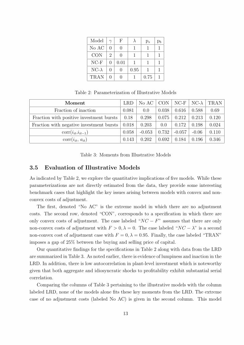
Table 2: Parameterization of Illustrative Models
Moment LRD No AC CON NC-F NC-λ TRAN
Fraction of inaction 0.081 0.0 0.038 0.616 0.588 0.69
Fraction with positive investment bursts 0.18 0.298 0.075 0.212 0.213 0.120
Fraction with negative investment bursts 0.018 0.203 0.0 0.172 0.198 0.024
corr(iit,iit−1) 0.058 -0.053 0.732 -0.057 -0.06 0.110
corr(iit, ait) 0.143 0.202 0.692 0.184 0.196 0.346
Table 3: Moments from Illustrative Models
3.5 Evaluation of Illustrative Models
As indicated by Table 2, we explore the quantitative implications of five models. While these
parameterizations are not directly estimated from the data, they provide some interesting
benchmark cases that highlight the key issues arising between models with convex and non-
convex costs of adjustment.
The first, denoted “No AC” is the extreme model in which there are no adjustment
costs. The second row, denoted “CON”, corresponds to a specification in which there are
only convex costs of adjustment. The case labeled “NC − F” assumes that there are only
non-convex costs of adjustment with F > 0, λ = 0. The case labeled “NC − λ” is a second
non-convex cost of adjustment case with F = 0, λ = 0.95. Finally, the case labeled “TRAN”
imposes a gap of 25% between the buying and selling price of capital.
Our quantitative findings for the specifications in Table 2 along with data from the LRD
are summarized in Table 3. As noted earlier, there is evidence of lumpiness and inaction in the
LRD. In addition, there is low autocorrelation in plant-level investment which is noteworthy
given that both aggregate and idiosyncratic shocks to profitability exhibit substantial serial
correlation.
Comparing the columns of Table 3 pertaining to the illustrative models with the column
labeled LRD, none of the models alone fits these key moments from the LRD. The extreme
case of no adjustment costs (labeled No AC) is given in the second column. This model
13
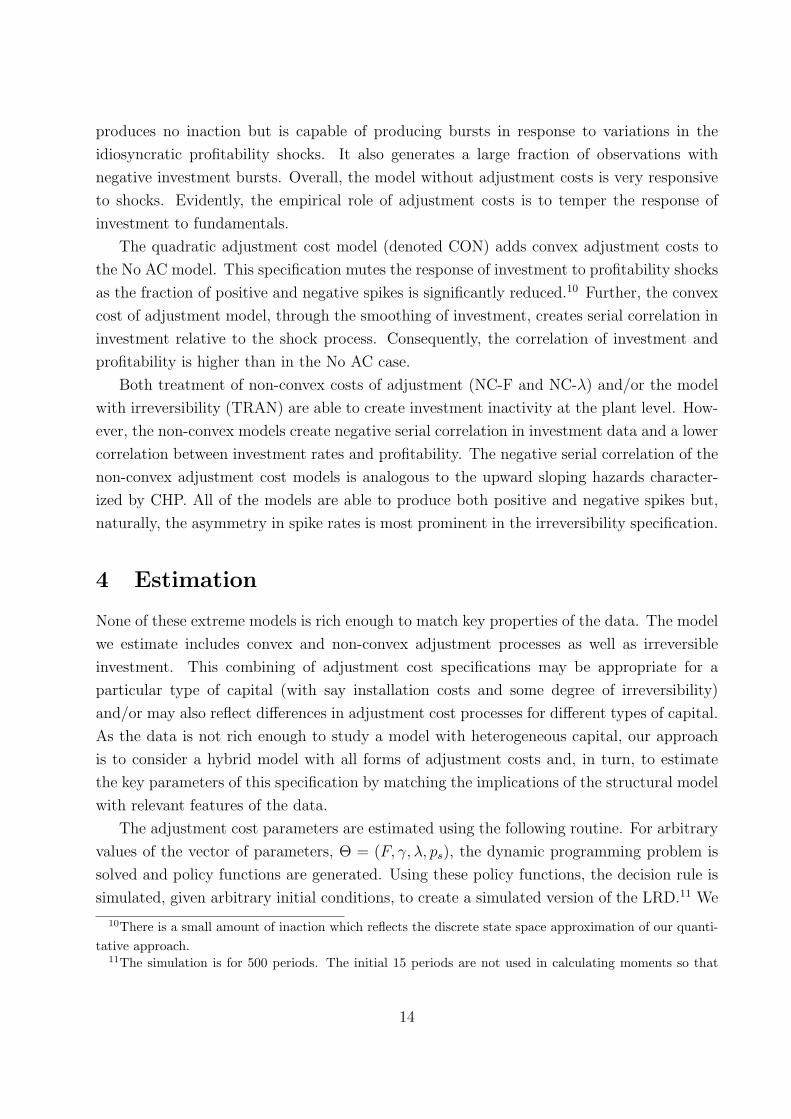
produces no inaction but is capable of producing bursts in response to variations in the
idiosyncratic profitability shocks. It also generates a large fraction of observations with
negative investment bursts. Overall, the model without adjustment costs is very responsive
to shocks. Evidently, the empirical role of adjustment costs is to temper the response of
investment to fundamentals.
The quadratic adjustment cost model (denoted CON) adds convex adjustment costs to
the No AC model. This specification mutes the response of investment to profitability shocks
as the fraction of positive and negative spikes is significantly reduced.10 Further, the convex
cost of adjustment model, through the smoothing of investment, creates serial correlation in
investment relative to the shock process. Consequently, the correlation of investment and
profitability is higher than in the No AC case.
Both treatment of non-convex costs of adjustment (NC-F and NC-λ) and/or the model
with irreversibility (TRAN) are able to create investment inactivity at the plant level. How-
ever, the non-convex models create negative serial correlation in investment data and a lower
correlation between investment rates and profitability. The negative serial correlation of the
non-convex adjustment cost models is analogous to the upward sloping hazards character-
ized by CHP. All of the models are able to produce both positive and negative spikes but,
naturally, the asymmetry in spike rates is most prominent in the irreversibility specification.
4 Estimation
None of these extreme models is rich enough to match key properties of the data. The model
we estimate includes convex and non-convex adjustment processes as well as irreversible
investment. This combining of adjustment cost specifications may be appropriate for a
particular type of capital (with say installation costs and some degree of irreversibility)
and/or may also reflect differences in adjustment cost processes for different types of capital.
As the data is not rich enough to study a model with heterogeneous capital, our approach
is to consider a hybrid model with all forms of adjustment costs and, in turn, to estimate
the key parameters of this specification by matching the implications of the structural model
with relevant features of the data.
The adjustment cost parameters are estimated using the following routine. For arbitrary
values of the vector of parameters, Θ = (F, γ, λ, ps), the dynamic programming problem is
solved and policy functions are generated. Using these policy functions, the decision rule is
simulated, given arbitrary initial conditions, to create a simulated version of the LRD.11 We
10There is a small amount of inaction which reflects the discrete state space approximation of our quanti-tative approach.
11The simulation is for 500 periods. The initial 15 periods are not used in calculating moments so that
14
then calculate a set of moments from the simulated data which we denote as Ψs(Θ). This
vector of moments depends on the vector of structural parameters, Θ, in a nonlinear way.
The estimate Θ minimizes the weighted distance between the actual and simulated mo-
ments. Formally, we solve
£(Θ) = minΘ
[Ψd −Ψs(Θ)]′W [Ψd −Ψs(Θ)] (6)
where W is a weighting matrix. This simulated method of moments procedure will generate
a consistent estimate of θ. We use the optimal weighting matrix given by an estimate of the
inverse of the variance-covariance matrix of the moments.12
Of course, the Ψs(Θ) function is not analytically tractable. Thus, the minimization is
performed using numerical techniques. Given the potential for discontinuities in the model
and the discretization of the state space, we used a simulated annealing algorithm to perform
the optimization.
For the estimation, we consider two specifications of non-convex adjustment costs. In
one, which we term the fixed cost case, the costs are represented by a lump-sum cost of
adjustment F > 0 without any opportunity costs of adjustment λ = 1. In the second,
which we term the opportunity cost case, F = 0 and λ < 1. These are taken as leading
specifications in the literature and thus our estimation provides insights into which is more
capable of capturing relevant features of the data.13
In addition to the adjustment cost parameters, the dynamic optimization problem is also
parameterized by the curvature of the profitability function and the process governing the
shocks to profitability. The two specifications of adjustment costs, particularly the presence
of a disruption effects, require different approaches to uncovering the underlying shocks to
profitability and characterizing the profitability function.
4.1 Estimation with Fixed Costs: F > 0 and λ = 1
Assume that the dynamic programming problem for a plant is given by:
V (A,K) = max{V b(A,K), V s(A,K), V i(A,K)} ∀(A,K) (7)
the results are independent of the assumed initial conditions. The moments are not sensitive to adding moreperiods to the simulation or to dropping more of the initial periods.
12See Smith [1993] for details of methodology and measurement of the weighting matrix. In our case, giventhe large micro dataset we use we estimate the moments that we are attempting to match very precisely. Assuch, most of the moments we are attempting to match receive a very large weight in (6).
13Caballero and Engel [1999] consider λ < 1 and F = 0 while Thomas [2002] assumes λ = 1 and F israndom.
15
where, as above, the superscripts refer to the act of buying capital ”b”, selling capital ”s”
and inaction ”i”. These options, in turn, are defined by:
V b(A,K) = maxI
Π(A,K)− FK − I − γ
2(I/K)2K + βEA′|AV (A′, K(1− δ) + I),
V s(A,K) = maxR
Π(A, K)− FK + psR− γ
2(R/K)2K + βEA′|AV (A′, K(1− δ)−R)
and
V i(A,K) = Π(A,K) + βEA′|AV (A′, K(1− δ)).
We have specified some parameters of the model (β = .95, δ = .069, pb = 1) for the
functional forms discussed above. Further, we retain our specification of the profit function,
Π(A,K) = AKθ. For the structural estimation, we focus on three parameters, Θ ≡ (F, γ, ps),
which characterize the magnitude of the non-convex and the convex components of the
adjustment process and the size of the irreversibility of investment. As explained next, we
estimate the curvature of the profit function and the A process independently of the dynamic
programming problem.
4.1.1 Estimates of θ and Measuring Profitability Shocks
Using the assumption of λ = 1, profits at plant i in period t are given by
Π(Ait, Kit) = AitKθit (8)
regardless of the level of investment activity. Suppose that ait ≡ ln(Ait) has the following
structure
ait = bt + εit (9)
where bt is a common shock and εit is a plant-specific shock. Assume εit = ρεεi,t−1 + ηit.
Taking logs of (8) and quasi differencing yields:
πit = ρεπit−1 + θkit − ρεθkit−1 + bt − ρεbt−1 + ηit (10)
We estimate this equation via GMM using a complete set of time dummies to capture
the aggregate shocks and using lagged and twice lagged capital and twice lagged profits as
instruments. To implement this estimation, real profits and capital stocks are calculated at
the plant-level. A more detailed discussion of the measurement of real profits and capital as
well as the estimation of the profit function and associated robustness issues are provided in
Appendix A. Our specification of the relatively simple AR(1) process for the idiosyncratic
16
shocks is motivated by the need to keep the state space relatively parsimonious for the
downstream numerical analysis and estimation.
The results give us an estimate of θ and an estimate of the process for the idiosyncratic
components of the profitability shocks. From the plant-level data, θ is estimated at 0.592
(0.006) and ρε is estimated at 0.885 (0.004).14 The estimate of θ is significantly below 1 and
this is interesting in its own right. Using the LRD plant-level data on cost shares we estimate
αL = .72 which implies a demand elasticity of -6.2 and a markup of about 16 %.15
Having estimated θ we recover ait from (8) and decompose it into aggregate and idiosyn-
cratic components using (9). This latter step amounts to measuring the aggregate shock as
the mean of ait in each year and the idiosyncratic shock as the deviation of ait from the year
specific mean. Using this decomposition we find that bt has a standard deviation of 0.08 and
with an AR(1) specification, the relevant AR(1) coefficient (denoted as ρb in what follows)
is given by 0.76 with a standard error of 0.19. We also find that the standard deviation of
εit is 0.64.
To sum up, in what follows, we use the following key estimates from the data in our
estimation of adjustment costs: θ = 0.592, σε = 0.64, ρε = 0.885, σb = 0.08, ρb = 0.76. These
were the parameter values used in section 3.5. These statistics imply that the innovations
to the aggregate shock process has a standard deviation of 0.05 and the innovations to the
idiosyncratic shock process have a standard deviation of 0.30. Neither process is estimated
to have a unit root.
These moments of the shock processes are critical for understanding the nature of ad-
justment costs since key moments, such as investment bursts, reflect the variability of prof-
itability shocks, the persistence of these shocks and the adjustment costs associated with
varying the capital stock. Moreover, the characterization of these processes provide the nec-
essary information for the solution of the plant level optimization problem which requires
the calculation of a conditional expectation of future profitability.
4.1.2 Estimates of (F, γ, ps)
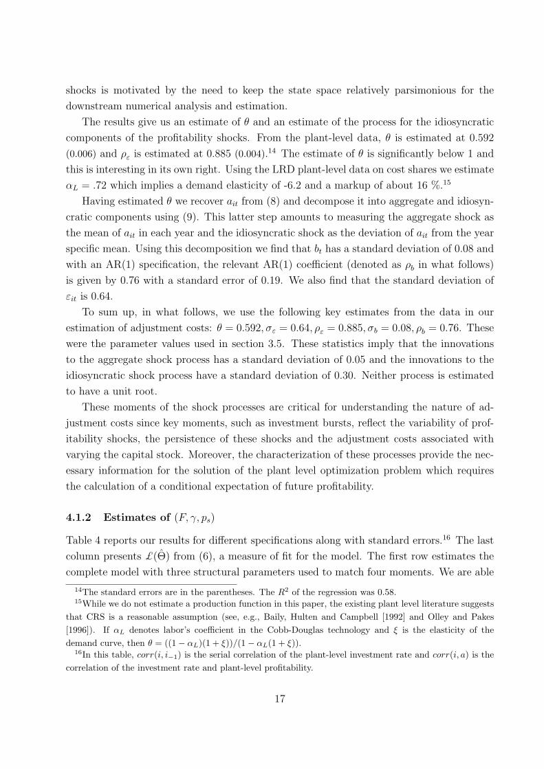
Table 4 reports our results for different specifications along with standard errors.16 The last
column presents £(Θ) from (6), a measure of fit for the model. The first row estimates the
complete model with three structural parameters used to match four moments. We are able
14The standard errors are in the parentheses. The R2 of the regression was 0.58.15While we do not estimate a production function in this paper, the existing plant level literature suggests
that CRS is a reasonable assumption (see, e.g., Baily, Hulten and Campbell [1992] and Olley and Pakes[1996]). If αL denotes labor’s coefficient in the Cobb-Douglas technology and ξ is the elasticity of thedemand curve, then θ = ((1− αL)(1 + ξ))/(1− αL(1 + ξ)).
16In this table, corr(i, i−1) is the serial correlation of the plant-level investment rate and corr(i, a) is thecorrelation of the investment rate and plant-level profitability.
17
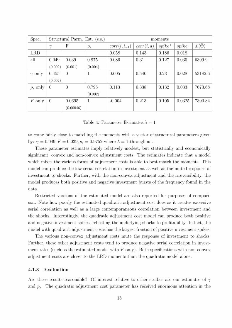
Spec. Structural Parm. Est. (s.e.) moments
γ F ps corr(i, i−1) corr(i, a) spike+ spike− £(Θ)
LRD 0.058 0.143 0.186 0.018
all 0.049 0.039 0.975 0.086 0.31 0.127 0.030 6399.9
(0.002) (0.001) (0.004)
γ only 0.455 0 1 0.605 0.540 0.23 0.028 53182.6
(0.002)
ps only 0 0 0.795 0.113 0.338 0.132 0.033 7673.68
(0.002)
F only 0 0.0695 1 -0.004 0.213 0.105 0.0325 7390.84
(0.00046)
Table 4: Parameter Estimates:λ = 1
to come fairly close to matching the moments with a vector of structural parameters given
by: γ = 0.049, F = 0.039, ps = 0.9752 where λ ≡ 1 throughout.
These parameter estimates imply relatively modest, but statistically and economically
significant, convex and non-convex adjustment costs. The estimates indicate that a model
which mixes the various forms of adjustment costs is able to best match the moments. This
model can produce the low serial correlation in investment as well as the muted response of
investment to shocks. Further, with the non-convex adjustment and the irreversibility, the
model produces both positive and negative investment bursts of the frequency found in the
data.
Restricted versions of the estimated model are also reported for purposes of compari-
son. Note how poorly the estimated quadratic adjustment cost does as it creates excessive
serial correlation as well as a large contemporaneous correlation between investment and
the shocks. Interestingly, the quadratic adjustment cost model can produce both positive
and negative investment spikes, reflecting the underlying shocks to profitability. In fact, the
model with quadratic adjustment costs has the largest fraction of positive investment spikes.
The various non-convex adjustment costs mute the response of investment to shocks.
Further, these other adjustment costs tend to produce negative serial correlation in invest-
ment rates (such as the estimated model with F only). Both specifications with non-convex
adjustment costs are closer to the LRD moments than the quadratic model alone.
4.1.3 Evaluation
Are these results reasonable? Of interest relative to other studies are our estimates of γ
and ps. The quadratic adjustment cost parameter has received enormous attention in the
18
literature since a regression of investment rates on the average value of the firm (termed
average Q) will identify this parameter when the profit function is proportional to K and the
cost of adjustment function is convex and homogenous of degree one. Using the Q-theoretic
approach, estimates of γ range from over 20 (Hayashi [1982]) to as low as 3 (Gilchrist-
Himmelberg [1995], unconstrained subsamples, bond rating).
Our estimates of γ = 0.049 appears extremely low relative to other estimates.17 Direct
comparison with other estimates should be viewed with caution given differences in methods
and datasets. Moreover, our best fitting model is the mixed model so it would be surprising
if our estimate of the convex costs are the same as that found by others as we are capturing
in other parameters what some studies are attempting to capture with only convex costs.
Note, however, that even if we use the estimate of γ from the γ only model that our estimate
of γ is low relative to those in the literature.
In addition, much of the literature uses a Q-theory approach and given the curvature in
the profit function in our analysis (recall we estimate θ = 0.59), the assumptions underlying
Q-theory do not hold. Put differently, the substitution of average for marginal Q produces
a measurement error. Following the arguments in Cooper-Ejarque [2001], this misspecifica-
tion of Q-theory based models implies that any inferences about the size of the quadratic
adjustment cost as well as the significance about financial variables may be invalid.
To study this latter point, we simulated a panel data set using our estimated model
with all forms of adjustment costs. From this data set and the associated values from the
dynamic programming problem, we constructed measures of expected discounted average
Q. We then regressed investment rates on these measures of average Q and then inferred
the value of γ from the regression coefficient on average Q. When γ = 0.049, along with
the other estimated parameters, is used in the simulation, the coefficient on average Q in a
regression of investment rates on a constant and average Q is very precisely estimated at 0.2
implying an estimate of γ = 5! Thus, the measurement error induced by replacing marginal
with average Q creates an inferred value of the quadratic adjustment cost parameter that is
well within the range of conventional estimates.18
Further, while others have considered models with non-convex costs of adjustment, there
17One exception is the recent study by Hall [2002] in which he estimates quadratic adjustment costs forboth labor and capital. Hall finds an average (across industries) value of 0.91 for γ and essentially noadjustment costs for labor.
18Essentially the substitution of average for marginal Q creates a negative correlation close to unitybetween the ”error” and average Q. Of course, this correlation goes to 0 if the profit function is proportionalto K. Cooper-Ejarque [2001] develop this point to argue that the same measurement error can explain thesignificance of profit rates in Q regressions in the absence of capital market imperfections. That same resultobtains here with non-convex adjustment costs: profit rates are also significant when added as a regressoralong with average Q.
19
are no estimates comparable to our estimate of the fixed cost.19 This estimate implies that
the fixed cost of adjustment is almost 4% of average plant level capital. This is a substantial
fixed cost.20
On ps, Ramey and Shapiro [2001] suggests that for some plants in the aerospace industry
that the value of ps is about 0.75 (this is based upon the resale prices of capital in this
industry). Our estimate is higher but one problem with making such a direct comparison
is that Ramey and Shapiro focused on plants that were being shut down. Our empirical
and theoretical analysis, in contrast, focuses exclusively on continuing plants. The nature
of irreversibility may be different for a continuing business compared to a business that is
shutting down. Understanding the nature of how adjustment costs vary between continuing
and entering and exiting plants is obviously an important topic for research in this area but
is beyond the scope of this paper. Another related problem for comparison is that Ramey
and Shapiro consider plants that shut down due to the shock associated with the end of
the Cold War and the fall of the Berlin Wall. For present purposes, we don’t believe the
Ramey-Shapiro estimates are directly comparable to our estimate of ps.
4.2 Estimation with Opportunity Costs: F = 0 and λ < 1
As other studies, such as Caballero-Engel [1999] and CHP, have introduced λ into the anal-
ysis, we broadened our empirical model to incorporate this type of non-convex adjustment
cost.21 With λ < 1, we capture any adjustment cost that disrupts the production process
through, for example, the shutting down of a production line or the reallocation of labor
from production to the installation of machines or training.
4.2.1 Estimates of θ and Measuring Profitability Shocks
Introducing λ < 1 implies that inferring profitability shocks and estimating θ separately
from the estimation of the adjustment costs is no longer possible. In particular, the presence
of λ in the production function implies that we must identify periods of low productivity
from periods of capital adjustment.
19In particular, neither CHP nor CEH estimate adjustment costs directly. Further, while fixed costs ofadjustment are present in the Abel and Eberly [1999] model they do not appear to be estimated either.
20As noted by a referee, one possible concern with our specification is that the fixed cost is proportionalto K and this will influence the investment decision. With this in mind, we estimated a version of the modelin which the fixed cost was proportional to the average capital stock of the plant. The resulting estimateswere F = 0.05, λ = 1, γ = 0.069, ps = 0.90 and £(Θ) = 6801.8. As the value of £(Θ) is higher for thisspecification, we focus on the model given in (7).
21In Caballero and Engel [1999], λ is treated as a random variable. This introduces an additional elementof plant-level heterogeneity that we do not consider. Instead, the plant-specific profitability shock interactswith a deterministic λ to create plant-specific adjustment costs.
20
One way to proceed would be to expand the set of moments to include the estimated
serial correlation and standard deviation of the aggregate and idiosyncratic shocks in the
set of moments. Then, for each vector of parameters we could re-estimate the moments for
the shocks following the methodology outlined in section 4.1.1. However, this would leave
results that were not directly comparable to those reported in Table 4.22
Instead, we adopted a two-step iterative procedure. We start with the curvature of
the profit function and the serial correlation and standard deviation of the aggregate and
idiosyncratic shock processes as directly estimated in section 4.1.1. We then proceed with
the best fit of the estimation of the adjustment cost parameters, including λ. We then
use the simulated data on profits and capital to estimate (10) and in so doing recover a
new estimate of the curvature and the shock processes based upon the simulated data. We
compare the latter estimates from the simulated data with the estimates of the curvature
and shock processes from the actual data using (10). If they match, we stop. If they don’t,
we adjust the curvature and shock processes and repeat the process. While in principle this
might take many iterations, in practice only very modest changes in the curvature and shock
processes are required to converge in one iteration.
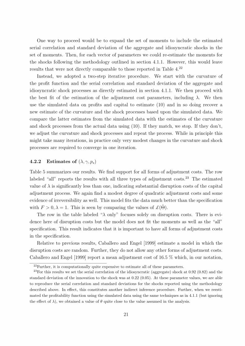
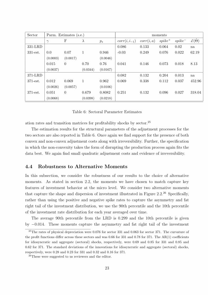
4.2.2 Estimates of (λ, γ, ps)
Table 5 summarizes our results. We find support for all forms of adjustment costs. The row
labeled “all” reports the results with all three types of adjustment costs.23 The estimated
value of λ is significantly less than one, indicating substantial disruption costs of the capital
adjustment process. We again find a modest degree of quadratic adjustment costs and some
evidence of irreversibility as well. This model fits the data much better than the specification
with F > 0, λ = 1. This is seen by comparing the values of £(Θ).
The row in the table labeled “λ only” focuses solely on disruption costs. There is evi-
dence here of disruption costs but the model does not fit the moments as well as the “all”
specification. This result indicates that it is important to have all forms of adjustment costs
in the specification.
Relative to previous results, Caballero and Engel [1999] estimate a model in which the
disruption costs are random. Further, they do not allow any other forms of adjustment costs.
Caballero and Engel [1999] report a mean adjustment cost of 16.5 % which, in our notation,
22Further, it is computationally quite expensive to estimate all of these parameters.23For this results we set the serial correlation of the idiosyncratic (aggregate) shock at 0.92 (0.82) and the
standard deviation of the innovation to the shock was at 0.22 (0.05). At these parameter values, we are ableto reproduce the serial correlation and standard deviations for the shocks reported using the methodologydescribed above. In effect, this constitutes another indirect inference procedure. Further, when we reesti-mated the profitability function using the simulated data using the same techniques as in 4.1.1 (but ignoringthe effect of λ), we obtained a value of θ quite close to the value assumed in the analysis.
21
Spec. Structural Parm. Est. (s.e.) moments
γ λ ps corr(i, i−1) corr(i, a) spike+ spike− £(Θ)
LRD 0.058 0.143 0.186 0.018
λ only 0 0.796 1.0 -0.009 0.06 0.107 0.042 9384.06
(0.0040)
all 0.153 0.796 0.981 0.148 0.156 0.132 0.023 2730.97
(0.0056) (0.0090) (0.0090)
Table 5: Parameter Estimates: F = 0
is a value of λ = 0.835. This latter value is quite close to ours which is striking given that
they estimate their model with industry-level data data while we estimate ours using micro
data. There are a number of subtle additional differences in methodology that may be at
work as well. Caballero and Engel assume that capital becomes immediately productive and
also have stochastic adjustment costs. Both of the latter imply lower average adjustment
costs which is consistent with the pattern of the estimated λ values across the studies.
To obtain a better sense of the magnitude of adjustment costs in this model, we simulated
the estimated policy functions and calculated the resulting costs of adjusting the capital
stock. The average adjustment cost paid relative to the capital stock was 0.0091 and was
0.031 as a fraction of profits.24
Though not reported in the table, we also estimated all four adjustment cost parameters,
Θ = (F, γ, λ, ps). We were unable to improve upon the fit summarized in Table 5: allowing
F > 0 did not enable us to better match the moments.
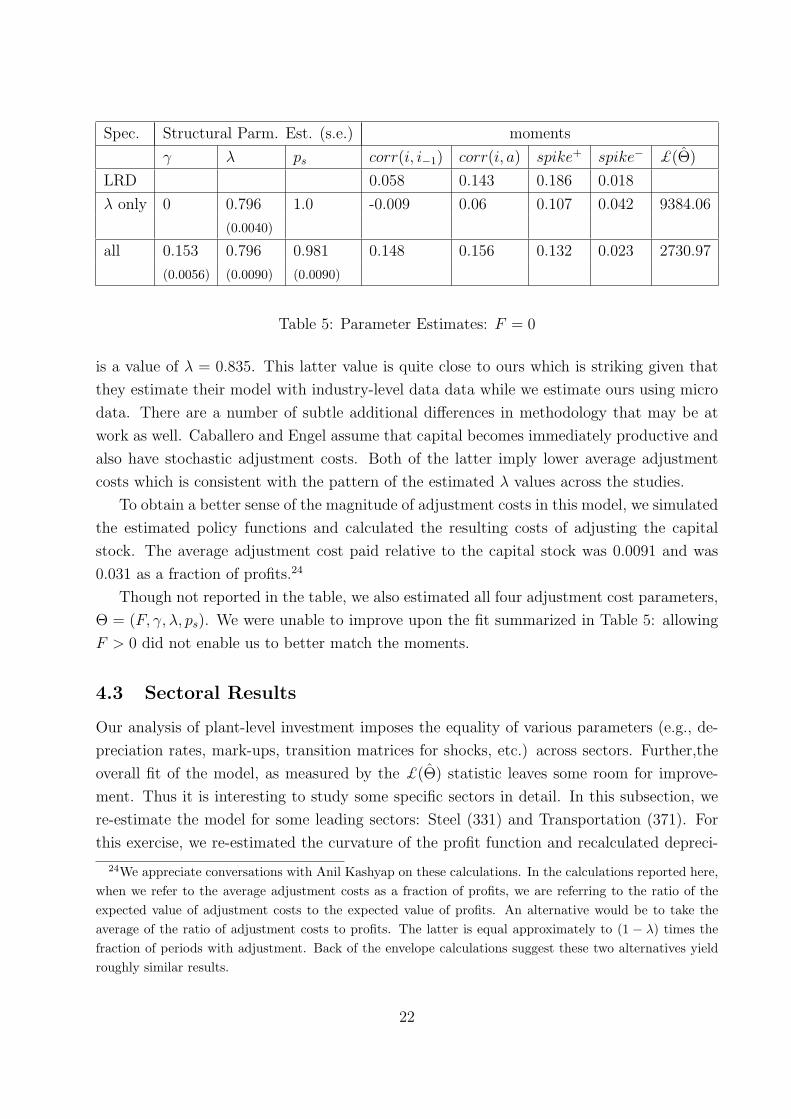
4.3 Sectoral Results
Our analysis of plant-level investment imposes the equality of various parameters (e.g., de-
preciation rates, mark-ups, transition matrices for shocks, etc.) across sectors. Further,the
overall fit of the model, as measured by the £(Θ) statistic leaves some room for improve-
ment. Thus it is interesting to study some specific sectors in detail. In this subsection, we
re-estimate the model for some leading sectors: Steel (331) and Transportation (371). For
this exercise, we re-estimated the curvature of the profit function and recalculated depreci-
24We appreciate conversations with Anil Kashyap on these calculations. In the calculations reported here,when we refer to the average adjustment costs as a fraction of profits, we are referring to the ratio of theexpected value of adjustment costs to the expected value of profits. An alternative would be to take theaverage of the ratio of adjustment costs to profits. The latter is equal approximately to (1 − λ) times thefraction of periods with adjustment. Back of the envelope calculations suggest these two alternatives yieldroughly similar results.
22
Sector Parm. Estimates (s.e.) moments
γ F λ ps corr(i, i−1) corr(i, a) spike+ spike− £(Θ)
331-LRD 0.086 0.133 0.064 0.02 na331-est. 0.0 0.07 1 0.946 -0.03 0.249 0.076 0.022 62.19
(0.0003) (0.0017) (0.0046)
0.015 0 0.70 0.76 0.041 0.146 0.073 0.018 8.13(0.0037) (0.0344) (0.0167)
371-LRD 0.082 0.132 0.204 0.013 na371-est. 0.012 0.069 1 0.962 0.069 0.338 0.112 0.037 452.96
(0.0026) (0.0057) (0.0106)
371-est. 0.051 0 0.679 0.8082 0.251 0.132 0.096 0.027 318.04(0.0068) (0.0398) (0.0218)
Table 6: Sectoral Parameter Estimates
ation rates and transition matrices for profitability shocks by sector.25
The estimation results for the structural parameters of the adjustment processes for the
two sectors are also reported in Table 6. Once again we find support for the presence of both
convex and non-convex adjustment costs along with irreversibility. Further, the specification
in which the non-convexity takes the form of disrupting the production process again fits the
data best. We again find small quadratic adjustment costs and evidence of irreversibility.
4.4 Robustness to Alternative Moments
In this subsection, we consider the robustness of our results to the choice of alternative
moments. As stated in section 2.2, the moments we have chosen to match capture key
features of investment behavior at the micro level. We consider two alternative moments
that capture the shape and dispersion of investment illustrated in Figure 2.2.26 Specifically,
rather than using the positive and negative spike rates to capture the asymmetry and fat
right tail of the investment distribution, we use the 90th percentile and the 10th percentile
of the investment rate distribution for each year averaged over time.
The average 90th percentile from the LRD is 0.299 and the 10th percentile is given
by −0.014. These moments capture the asymmetry and fat right tail of the investment
25The rates of physical depreciation were 0.076 for sector 331 and 0.063 for sector 371. The curvature ofthe profit functions differ across these sectors and was 0.66 for 331 and 0.78 for 371. The AR(1) coefficientsfor idiosyncratic and aggregate (sectoral) shocks, respectively, were 0.69 and 0.85 for 331 and 0.85 and0.62 for 371. The standard deviations of the innovations for idiosyncratic and aggregate (sectoral) shocks,respectively, were 0.28 and 0.23 for 331 and 0.32 and 0.16 for 371.
26These were suggested to us reviewers and the editor.
23
distribution. When we use these two moments along with the two correlation moments in
our analysis, the estimated adjustment cost parameters are qualitatively and quantitatively
similar to the parameter estimates reported in Table 5. That is, matching these alternative
moments requires a relatively modest convex cost component and substantial disruption
adjustment costs and transaction adjustment costs. To be specific, the best fit for matching
this alternative set of moments implies an estimate of γ = 0.042, λ = 0.86 and ps = 0.80.
These parameter estimates yield simulated moments of: corr(i, i−1) = 0.033, corr(i, a) =
0.133, the average 90th percentile investment rate of 0.308, and the average 10th percentile
investment rate equal to 0.00. As these alternative moments are estimated precisely in the
actual data, the adjustment cost parameters are as tightly estimated as those in Table 5.
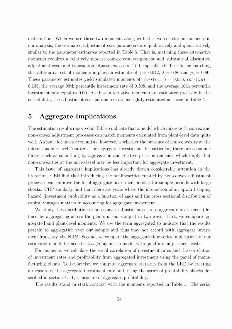
5 Aggregate Implications
The estimation results reported in Table 5 indicate that a model which mixes both convex and
non-convex adjustment processes can match moments calculated from plant-level data quite
well. An issue for macroeconomists, however, is whether the presence of non-convexity at the
microeconomic level “matters” for aggregate investment. In particular, there are economic
forces, such as smoothing by aggregation and relative price movements, which imply that
non-convexities at the micro-level may be less important for aggregate investment.
This issue of aggregate implications has already drawn considerable attention in the
literature. CEH find that introducing the nonlinearities created by non-convex adjustment
processes can improve the fit of aggregate investment models for sample periods with large
shocks. CHP similarly find that there are years where the interaction of an upward sloping
hazard (investment probability as a function of age) and the cross sectional distribution of
capital vintages matters in accounting for aggregate investment.
We study the contribution of non-convex adjustment costs to aggregate investment (de-
fined by aggregating across the plants in our sample) in two ways. First, we compare ag-
gregated and plant-level moments. We use the term aggregated to indicate that the results
pertain to aggregation over our sample and thus may not accord with aggregate invest-
ment from, say, the NIPA. Second, we compare the aggregate time series implications of our
estimated model, termed the best fit, against a model with quadratic adjustment costs.
For moments, we calculate the serial correlation of investment rates and the correlation
of investment rates and profitability from aggregated investment using the panel of manu-
facturing plants. To be precise, we compute aggregate statistics from the LRD by creating
a measure of the aggregate investment rate and, using the series of profitability shocks de-
scribed in section 4.1.1, a measure of aggregate profitability.
The results stand in stark contrast with the moments reported in Table 1. The serial
24
correlation of aggregate investment is 0.46 and the correlation between investment and the
profitability shock is 0.51 for the aggregated data. In contrast, the plant-level data exhibits
much less serial correlation, 0.058, and much less contemporaneous correlation between in-
vestment and shocks, 0.143.
How well does the best fit model match these aggregate facts? If we compute aggregate
investment and the aggregate shock from a simulation using the best fit model, the serial
correlation of aggregate investment is 0.63 and the correlation between investment and the
profitability shock is 0.54. Thus aggregation of the heterogeneous plants alone substantially
increases both the serial correlation of investment and its correlation with profitability.
In fact, the aggregate moments reported above seem to be much closer to the prediction
of a quadratic cost of adjustment model: from Table 3, a model with quadratic adjustment
costs implies high serial correlation and high contemporaneous correlation of investment and
shocks. This suggests a second exercise in which we ask how well a quadratic adjustment
cost model can match the aggregate data created by the estimated model. To study this,
we created a time series simulation (periods) for the estimated model. We then searched
over quadratic adjustment costs models to find the value of γ to maximize the R2 between
the series created by the best fit model and that created by the quadratic model. A value
of γ = 0.195 solved this maximization problem and the R2 measure was 0.859. Thus the
quadratic model explains most but not all of the time series variation from the best fit model.
This analysis of the aggregate implications is potentially incomplete in that we ignore
two important factors. First, we do not explicitly consider general equilibrium effects.27 As
emphasized by Veracierto [2002], Caballero [1999] and Thomas [2002], it is likely that there
is further smoothing by aggregation due to the congestion effects that are potentially present
in the capital goods supply industry and/or due to endogenous interest rate fluctuations.
Second, we work with a sub-set of manufacturing plants. In particular, we have selected
a balanced panel and thus ignored entry and exit, including the investment associated with
that decision. Thus our “aggregate results” refer to the aggregation over a fixed set of plants.
Nonetheless, the analysis uncovers strong effects of smoothing over heterogeneous plants
without variations in relative prices. While identifying the mechanisms that smooth out
plant-specific non-convexities is of interest, it should be clear that both smoothing by aggre-
gation and variations in factor prices are important to the smoothing process. That said, it is
also clear that the non-convexities at the plant-level are not totally smoothed by aggregation:
our goodness of fit measure is 0.859 not 1!
27Recall that we have been able to identify the adjustment costs using cross sectional differences in invest-ment dynamics across plants having controlled for aggregate shocks. However, even though we have beenable to identify the adjustment costs, aggregate variation in investment will reflect the complex interactionof shocks, endogenous factor prices, and adjustment dynamics.
25
6 Conclusions
The goal of this paper is to analyze capital dynamics through competing models of the
investment process: what is the nature of the capital adjustment process? The methodology
is to take a model of the capital adjustment process with a rich specification of adjustment
costs and solve the dynamic optimization problem at the plant level. Using the resulting
policy functions to create a simulated data set, the procedure of indirect inference is used to
estimate the structural parameters.
Our empirical results point to the mixing of models of the adjustment process. The LRD
indicates that plants exhibit periods of inactivity as well as large positive investment bursts
but little evidence of negative investment. The resulting distribution of investment rates at
the micro level is highly skewed even though the distribution of shocks is not. A model which
incorporates both convex and non-convex aspects of adjustment, including irreversibility, fits
these observations best. In particular, a model of adjustment in which the non-convex cost
entails the disruption of production fits the data best.
In terms of further consideration of these issues, we plan to continue this line of research
by introducing costs of employment adjustment. This is partially motivated by the ongoing
literature on adjustment costs for labor as well as the fact that the model without labor
adjustment costs implies labor movements that are not consistent with observation.
Further, it would be insightful to utilize this model to study the effects of investment
tax subsidies. Here those subsidies enter quite easily through policy induced variations in
the cost of capital. Clearly, one of the gains to structural estimation is to use the estimated
parameters for policy analysis. An interesting aspect of that exercise will be a comparison
of the estimated model and a quadratic adjustment cost model in terms of their predictions
of the aggregate effects of an investment tax credit.
Finally, there are some methodological issues worth exploring further. For this exercise,
we have chosen to estimate the model using a simulated method of moments approach.
There are, of course, competing approaches, including maximum likelihood estimation as
well as estimation from the Euler equations, including periods of inaction. In future research,
we plan on exploring these competing approaches. These alternative approaches have the
potential advantage in that they do not rely on matching specific moments but rather can
confront the micro data directly.
Still, it is useful to emphasize that the simulated method of moments approach we use
here has a number of distinct advantages especially in this context. First, structural models
of investment with non-convex adjustment costs obviously imply a range of inaction. In
the actual micro data, while we do observe some range of inaction as we report in Table
1, the more robust finding is that the distribution of investment is skewed and kurtotic
with a mass around zero and a fat right tail. Identifying inaction precisely at the micro
26
level is difficult because in practice there is substantial heterogeneity in capital assets with
associated heterogeneity in adjustment costs. For example, buying a specific tool gets lumped
into capital equipment expenditures in the same way as retooling the entire production
line. The former presumably has little or no adjustment costs while the other is subject
to presumably high adjustment costs. The implication is that in pursuing MLE or Euler
equation estimation using the actual micro data a researcher must define “inaction” without
observing the underlying capital heterogeneity. Specifically, should a researcher identify
inaction as literally zero investment or small investment expenditures that reflect “buying a
wrench”?28 In contrast, we exploit robust moments of the investment and profit distributions.
While we believe the moments we match are robust to capital heterogeneity, this discus-
sion reminds us of the limitations of even high quality micro data such as the LRD. The
class of adjustment cost models we focus on in this paper are best interpreted as applying
to variations in capital expenditures that are relatively homogenous in type. It is unlikely
we will have a rich longitudinal micro data-set on establishments with annual data on cap-
ital expenditures by detailed asset class, unobserved heterogeneity in capital is a feature of
reality that estimation of investment dynamics with micro data on plants needs to confront
regardless of the methodology used.
Another strength of our approach is that analysis and estimation does not require direct
and continuous access to the micro data. Given that virtually all of the high quality longi-
tudinal micro datasets are proprietary, it is very useful to have methods available that can
take advantage of moments from the micro data that can be analyzed off-site. The research
community at large has a much better chance of exploring alternative models of investment
using the simulated method of moments approach given limited direct access to the micro
data. Our findings suggest there would be considerable value to statistical agencies pro-
ducing summary measures of the distributions of micro investment behavior and its auto
covariance and cross covariance with other micro measures.
In the end, there are many dimensions to improve the match between the models we spec-
ify and estimate and the full richness of the actual micro data. Despite these limitations,
we have identified features of the micro data that can only be reconciled with models that
contain both convex and nonconvex adjustment costs. In particular, a modest convex com-
ponent and substantial transaction and disruption costs are required to capture key features
of micro investment.
28In related earlier work, Cooper, Haltiwanger and Power [1999] took a stand on this by defining investmentspikes of investment greater than 20 percent as the investment that is subject to fixed adjustment costs.They investigated the robustness of this admittedly ad hoc threshold but noted that this was a limitationof their analysis.
27
Appendix A
In this section, we discuss the measurement of key variables and the details and robustness of
estimation for the profit function. Real variable profits are measured as revenue less variable
costs (labor and material) deflated by the GDP implicit price deflator for consumption. We
make the assumption that measured real variable profits provide an estimate of Π(A,K) =
λAKθ in the model . The question then is how adjustment costs in the model are captured in
the measured real variable profits or other cost measures in the data. We think it is reasonable
to assume that some part of capital adjustment costs are reflected in real variable measured
profits either due to the disruption of productivity and/or perhaps equivalently that some
of the labor that might have normally been used for production is used for installing capital.
It is precisely these arguments that motivate us to consider including an adjustment cost
factor via λ. We also think it is reasonable to assume that some adjustment costs take the
form of purchased services or contract work that are not captured in measured real variable
profits. It is precisely these arguments that motivate us to include adjustment costs that
are additively separable from real variable profits and may be either convex or nonconvex
in nature – hence we consider adjustment costs in the form of both γ or F . In terms of
measurement in the LRD, there are not annual data on such purchased services or contract
work and so we cannot directly measure these costs. However, we can infer the presence of
these costs through the dynamics of investment.
As described in the text, we estimate the parameters of the real variable profit function
using the quasi-differenced (10). In practice, we use a transformed version of (10) taking
advantage of assumptions that the production function is Cobb-Douglas and that the demand
function has constant elasticity. Specifically, we assume that the plant faces an inverse
demand function given by p = y−η and so has a revenue function of R(y) = y1−η. Assuming
that the production function is given by y = AKαLφ and that K is predetermined, L is the
variable factor(s) and ω is the price of the variable factor(s). The equations that follow are
based on one variable factor for expositional purposes but extend easily to multiple variable
factors and in our case there are two: labor and materials. Optimization over the variable
factor yields a revenue function R(K,A, ω), a profit function π(K,A, ω) and variable factor
demand of L = h(K, A, ω). The implied revenue and profit functions are given by:
R(K,A, ω) = A1
1−φ Kα
1−φ
(ω
φ
) φ
φ−1
(11)
π(K, A, ω) = (1− φ)A1
1−φ Kα
1−φ
(ω
φ
) φ
φ−1
. (12)
where α = α(1− η) and φ = φ(1− η). So the coefficient on k in both the revenue
28

and profit functions is the same,given by θ = α1−φ
. Moreover, the properties of the shocks
to revenue and profits are the same up to a factor of proportionality. So the estimation
strategy is to estimate θ from either a quasi-differenced profit or revenue regression on the
capital stock. The latter seems preferred since there is potentially less measurement error
involved. There are a small number of observations with negative measured real variable
profits but by construction there are no businesses with negative real revenue. While it
may be that negative real variable profits is possible we suspect that this largely reflects
measurement error. To explore this issue we estimated the log linear quasi-differenced real
revenue function on all observations and the log linear quasi-differenced real profit function
on only those observations with non-negative real variable profits. We obtained very similar
estimates of θ using both approaches. In the analysis in the paper we use the estimate of
θ from the real revenue quasi-differenced estimation but this is not critical for the reported
results.
To obtain the profit shocks, we use the estimate of θ and use (12) to infer the shock.
We decompose the shock into aggregate and idiosyncratic components (the aggregate shock
is the first moment of the profit shock in any given year and the idiosyncratic shock is the
residual after controlling for year effects). We then estimate the properties of the aggregate
and idiosyncratic shocks (both the degree of first order autocorrelation and the variance of
the innovations). We note again that the properties of these shocks are quite similar across
alternative ways of estimating θ.
To provide a sense of the robustness of both the estimates of θ as well as the properties
of the shocks, we performed a number of cross-checks. One cross-check that we perform is
that the above procedures yield two alternative estimates of ρε – one estimate is as described
from inferring the shock from the profit function and the second is from the estimation of
the quasi-differenced revenue function. These two estimates of ρε are very similar to each
other providing support for this estimation strategy.
As a second cross-check, we explored the properties of the innovations to this first-order
process. We found that the innovations to the AR(1) representation of εit had a serial
correlation very close to zero (-0.05).
In addition, as a check on the robustness of our estimate of θ, we also estimated AR(2)
specifications with appropriate second quasi-differencing in our estimation of θ. We found θ
was 0.60 when we assumed an AR(2) compared to the estimate of 0.592 reported in the text
with the AR(1) specification. There was essentially no improvement in the overall fit of the
model with an AR(2) specification. Interestingly, even for the OLS estimation we obtained
an estimate of θ of 0.591. Thus, the estimate of θ is very robust. As noted above, once we
have an estimate of θ (which is apparently very robust), the properties of the aggregate and
idiosyncratic shocks are well captured by an AR(1) process (e.g., the implied innovations are
29

serially uncorrelated).
We note in closing that is it not uncommon in the firm-level literature to assume a
first order process for the underlying shocks. For example, the Olley and Pakes [1996] and
Levinsohn and Petrin [2000], hereafter LP, methods for estimating production functions are
based on the assumption of first order Markov processes. A key difference between the
approach in their papers and that pursued here is that they use a more general first order
Markov process. For example, LP specify the first order process as the productivity shock in
period t being a polynomial function of the productivity shock in t-1. As a further point of
comparison, unlike these papers we are not seeking to identify the factor elasticities of both
variable and quasi-fixed factors of production. Rather, we seek to identify the coefficient on
the quasi-fixed factor in the profit function after having already maximized out the variable
factors of production. As such, we are similar to LP’s “second stage” where they identify the
coefficient on capital. In LP’s second stage, they employ a GMM approach with lagged values
of inputs as instruments in a manner similar to that employed here (although again with the
polynomial specification for the first order process their estimation is more complex).
30
References
[1] Abel, A. and J. Eberly, “A Unified Model of Investment under Uncertainty,” American
Economic Review, 84 (1994), 1369-84.
[2] Abel, A. and J. Eberly, “Optimal Investment with Costly Reversibility,” Review of
Economic Studies, 63 (1996), 581-93.
[3] Abel, A. and J. Eberly, ”The Mix and Scale of Factors with Irreversibility and Fixed
Costs of Investment,” NBER Working Paper # 6148, 1997.
[4] Abel, A. and J. Eberly, “Investment and q with Fixed Costs: An Empirical Analysis,”
mimeo, April 1999.
[5] Caballero, R., “Aggregate Investment,” in Handbook of Macroeconomics, (edited by J.
Taylor and M. Woodford), Amsterdam: North Holland, 1999.
[6] Caballero, R. and E. Engel, “Explaining Investment Dynamics in U.S. Manufacturing:
A Generalized (S,s) Approach, ” Econometrica, 67 (1999), 783-826.
[7] Caballero, R. and E. Engel, ”Adjustment Is Slower Than You Think,” NBER Working
Paper No. 9898, August 2003.
[8] Caballero, R., E. Engel and J. Haltiwanger, “Plant-level Adjustment and Aggregate
Investment Dynamics,” Brookings Papers on Economic Activity, 2 (1995), 1-39.
[9] Caballero, R., E. Engel and J. Haltiwanger, “Aggregate Employment Dynamics: Build-
ing from Microeconomic Evidence,” American Economic Review 87 (1997), 115-37.
[10] Cooper, R. and J. Ejarque, “Exhuming Q: Market Power vs.Capital Market Imperfec-
tions” NBER Working Paper No. 8182, March 2001.
[11] Cooper, R. and J. Haltiwanger, “The Aggregate Implications of Machine Replacement:
Theory and Evidence,” American Economic Review, 83 (1993), 360-82.
[12] Cooper, R., J. Haltiwanger and L. Power, “Machine Replacement and the Business
Cycle: Lumps and Bumps,” American Economic Review, 89 (1999), 921-46.
[13] Doms, M. and T. Dunne,“Capital Adjustment Patterns in Manufacturing Plants,” Cen-
ter for Economic Studies, U.S. Bureau of the Census, 1994.
[14] Gilchrist, S. and C. Himmelberg, “The Role of Cash Flow in Reduced-Form Investment
Equations,” Journal of Monetary Economics, 36 (1995), 541-72.
31
[15] Gilchrist, S. and C. Himmelberg, “Investment, Fundamentals and Finance,” The NBER
Macroeconomics Annual, 1998.
[16] Goolsbee, A. “The Business Cycle, Financial Performance and the Retirement of Capital
Goods,” NBER Working Paper #6392, February 1998.
[17] Goolsbee, A. and D. Gross, “Estimating Adjustment Costs with Data on Heterogeneous
Capital Goods,” NBER Working Paper #6342, December 1997.
[18] Hall, R. “Industry Dynamics with Adjustment Costs,” NBER Working Paper #8849
March 2002.
[19] Hamermesh, D. “Labor Demand and the Structure of Adjustment Costs,” American
Economic Review, 79 (1989), 674-89.
[20] Hamermesh, D. and G. Pfann, “Adjustment Costs in Factor Demand,” Journal of Eco-
nomic Literature, 34 (1996), 1264-92.
[21] Hayashi, F. “Tobin’s Marginal and Average q: A Neoclassical Interpretation,” Econo-
metrica 50 (1982), 213-24
[22] Holt, C., F. Modigliani, J. Muth, and H. Simon, Planning Production, Inventories, and
Work Force, Englewood Cliffs, N.J.: Prentice-Hall, 1960.
[23] Huggett, M and S. Ospina, “Does Productivity Fall After the Adoption of New Tech-
nology?” Journal of Monetary Economics 48 (2001), 173-95.
[24] Ito, H., T. Bresnahan and S. Greenstein, “The Sources and Effects of Investment Irre-
versibility: Large Scale Computing,”, mimeo, 1999.
[25] Khan, A. and J. Thomas, “Nonconvex Factor Adjustments in Equilibrium Business
Cycle Models: Do Nonlinearities Matter?”, Journal of Monetary Economics, 50 (2003),
331-60.,
[26] Levinsohn, J. and A. Petrin,“Estimating Production Functions Using Inputs to Control
for Unobservables,” NBER Working Paper #7819, August 2000.
[27] Nilsen, O. and F. Schiantarelli, “Zeroes and Lumps in Investment: Empirical Evidence
on Irreversibilities and nonconvexities,” mimeo, Boston College, March 1998.
[28] Olley, G.S. and A. Pakes, “The Dynamics of Productivity in the Telecommunications
Equipment Industry,” Econometrica, 64 (1996) 1263-97.
32
[29] Peck, S. “Alternative Investment Models for firms in the Electric Utilities Industry,”
Bell Journal of Economics and Management Science, 5 (1974), 420-57.
[30] Power, L. “The Missing Link: Technology, Investment and Productivity,” Review of
Economics and Statistics, 80 (1998), 300-13.
[31] Ramey, V. and M. Shapiro, “Displaced Capital,” Journal of Political Economy, 109
(2001), 958-92.
[32] Rothschild, M. “On the Cost of Adjustment,” Quarterly Journal of Economics 85
(1971), 605-22.
[33] Sakellaris, P. ”Patterns of Plant Adjustment,” Working Paper #2001-05, Finance and
Economics Discussion Series, Division of Research and Statistics and Monetary Affairs,
Federal Reserve Board, Washington D.C., 2001.
[34] Smith, A. “Estimating Nonlinear Time-Series Models Using Simulated Vector Autore-
gressions,” Journal of Applied Econometrics, 8 (1993), S63-S84.
[35] Tauchen, G. “Finite State Markov-Chain Approximation to Univariate and Vector Au-
toregressions”Economics Letters, 20 (1986), 177-81.
[36] Thomas, J., “Is Lumpy Investment Relevant for the Business Cycle?” Journal of Polit-
ical Economy, 110 (2002), 508-34.
[37] Veracierto, M. “Plant Level Irreversible Investment and Equilibrium Business Cycles,”
American Economic Review, 92 (2002), 181-97.
33


