
Numerical study on a KVLCC2 model advancing in shallow water
Zhi-Ming Yuan, Paula Kellett
Department of Naval Architecture, Ocean and Marine Engineering
University of Strathclyde, Glasgow, UK
Abstract: Due to the effects from the bottom of the waterway, advancing ships will sink deeper in shallow
water than in deep water. This is known as squat effect, which increases with the speed of the vessel. The
aim of the present paper is to provide a numerical method to predict the shallow water effects. The 3-D
boundary element method is firstly applied to simulate a KVLCC2 model advancing in confined water. The
wave-making resistance, as well as the sinkage and trim are calculated at different water depths. In order to
verify the predictions from BEM program, CFD calculations in deep water will also be conducted and
compared. Special efforts are made to calculate the wave elevations. The wave profiles at different water
depths and distances are calculated. The comparisons between shallow water and deep water, as well as
between the BEM and CFD programs, are also discussed in the present paper. Additionally, some
comparison of the wave profiles with available experimental results is presented for validation of the
approaches.
Key words: Shallow water effects; Squat; Boundary element method; CFD; Wave patterns; KVLCC2
1 Introduction
The shallow water problem remains a challenging topic in the seakeeping and manoeuvring field. When a
ship moves through the shallow water, the following changes are observed to occur on the vessel presumably
due to squat (Varyani, 2006): 1) increase in vessel’s wave-making; 2) reduction in speed of the vessel due
to increase in resistance; 3) reduction in propeller rpm compared to that in deep water conditions; 4)
reduction in course-changing ability of the vessel; 5) vibrations on the vessel due to the entrained water
effect. The influence of limited water depth on the ship motions becomes obvious when the water depth is
less than 4 times the draft of the vessel. When the ratio of water depth to draft is less than 2, the effect of the
bottom becomes significant (Van Oortmerssen, 1976).
Published work on the effect of water depth can be found in Kim (1969), Tuck (1970) and Andersen (1979).
Most of them were based on the slender body assumption and no consideration of free-surface was involved
when solving a two-dimensional problem. Varyani (2006) investigated the squat effects on high speed craft
in restricted waterways and found that the effects of squat were magnified in shallow water and restricted
waterways and the blockage effects were significant when W/L=1. Yao and Zou (2010) used a constant
Rankine source panel method to predict ship squat in restricted waterways. Calculations were performed for
a Series 60 (CB=0.6) ship in a shallow channel. Their method was verified by comparisons between the
calculated results and available experimental data. It was shown that the proposed numerical method can
predict sinkage and trim with a satisfactory accuracy for a ship advancing in a shallow channel at subcritical
and supercritical speeds, but it was unable to obtain convergent results for the ship travelling near the critical
speed range. Lataire et al. (2012) proposed a prediction method based on an equivalent width for the squat
of vessels advancing in restricted and unrestricted rectangular fairways. Their mathematical model took
account of the magnitude and distribution of the cross-sectional areas of the vessel as well as the longitudinal
distribution of the beam on the water line of the vessel. The fairway could vary from an infinitely open ocean
(water depth and width infinite) to an extremely restricted channel in width and water depth with a
rectangular cross section. However, their method was only validated against rectangular cross sections.
In the present study, we present a numerical program (MHydro) based on a 3D Rankine source method, to
predict the shallow water effects on vessels advancing in calm water. Calculations for a KVLCC2 model
will be conducted by using both of the BEM and CFD programs. The wave-making resistance, as well as the sinkage and trim are calculated at different water depths by using MHydro. The special efforts are made to

calculate the wave elevation. The wave profiles at different water depth are calculated. The comparisons
between shallow water and deep water are also discussed in the present paper based on BEM.
2 Mathematical formulation of MHydro
2.1 The boundary value problem
When a ship advances at constant speed in calm water, it will generate steady waves and induce the so-called
wave-making resistance. It is assumed that the fluid is incompressible and inviscid and the flow is irrotational.
A velocity potential T ux is introduced and φ satisfies the Laplace equation
2 0 in the fluid domain (1)
Following Newman (1976), the nonlinear dynamic free-surface condition on the disturbed free surface can
be expressed as
22 21
0, ( , )2
u g on z x yx x y z
(2)
The kinematic free-surface condition is
0, ( , )u on z x yx z y y x x
(3)
The first approximation is based on the linear free surface conditions on the undisturbed water
surface. By neglecting the nonlinear terms in Eq. (2) and (3), we can obtain the linear classic free
surface boundary condition
2
2
20u g
zx
, on the undisturbed free surface (4)
For the ship-to-ship with same forward speed problem, the body surface boundary condition can be written
as
1u nn
, on the wetted body surface (5)
where 1 2 3( , , )n n nn is the unit normal vector inward on the wetted body surface of Ship_a and Ship_b.
The boundary condition on the sea bottom and side walls can be expressed as
0n
, on z = -h and side walls (6)
Besides, a radiation condition is imposed on the control surface to ensure that the waves vanish upstream of
the disturbance.
2.2 Forces and wave elevation
Once the unknown potential φ is solved, the pressure on the vessel can be obtained from Bernoulli’s equation:
22 21
2p u
x x y z
(7)
where ρ is the fluid density. The forces on the ship can be written as
i i
S
F pn ds , i =1, 2, …, 6 (8)

where
, 1,2,3
, 4,5,6i
in
i
n
x n (9)
The mean sinkage σ and trim τ can be written as
3 / ws F gA (10)
5 / wt F gI (11)
Where Aw is the water plane area and Iw is second moment of the water plane about the y-axis.
The wave elevation on the free surface can then be obtained from the dynamic free surface boundary
condition in the form
22 21
2
u
g x g x y z
(12)
2.3 Numerical implementation
In the numerical study, the boundary is divided into a number of quadrilateral panels with constant source
density σ(i) (i=1,2,…,N), where N is the panel number. The potential at the ith panel (the centroid coordinate
can be denoted as (xi, yi, zi)) induced by the jth panel (the centroid coordinate can be denoted as (xj, yj, zj))
can be expressed by
, , , , 1,2,...,i j i j jG i j N (13)
where denotes the steady potential s or the unsteady potential j , Gi, j is the Rankine-type Green
function that satisfies the sea bed boundary condition through the method of mirror image
,2 2 2 2 2 2
1 1
( ) ( ) ( ) ( ) ( ) ( 2 )i j
i j i j i j i j i j i j
Gx x y y z z x x y y z d z
(14)
When the ith panel and the jth panel are close to each other, Gi, j can be calculated with analytical formulas
listed by Prins (1995). When the distance between the ith panel and the jth panel is large, these coefficients
are calculated numerically. The same procedure can be applied to discretize the boundary integral for the
normal derivative of the potential
,
, ,
i jn ni j j i j j
i
GG
n
(15)
Similarly, the derivative of the potential to x and z can be written as
,
, ,
i jx xi j j i j j
i
GG
x
(16)
,
, ,
i jz zi j j i j j
i
GG
z
(17)
The analytical formulas of the influence coefficients ,ni jG , ,
xi jG and ,
zi jG are listed by Hess and Smith (1964).
Special attention should be paid to the second derivative of the potential on the free surface. Generally, the
differencing schemes can be divided into two classes: upwind difference schemes and central difference
schemes. Although central difference schemes are supposed to be more accurate, the stabilizing properties

of the upwind difference schemes are more desirable in the forward speed problem (Bunnik, 1999).
Physically this can be explained by the fact that new information on the wave pattern mainly comes from
the upstream side, especially at high speeds, whereas the downstream side only contains old information.
The first-order upwind difference scheme for the second derivative of the potential to x can be written as
follows
, , 2 , 1 ,2
12xx
i j i j i j i j
jx
(18)
By substituting Eq.(13), (15)-(18) into the body-, free- and control-surface boundary conditions, the
following set of linear equations for the values of the source density can be obtained
,
1
, 1,2,...,N
i j j i
j
P Q i N
(19)
It should be noted that the singularity distribution does not have to be located on the free surface itself, it can
also be located at a short distance above the free surface, as long as the co-location points, where the
boundary condition has to be satisfied, stay on the free surface. In practice, a distance of maximum three
times the longitudinal size of a panel is possible (Bunnik, 1999). In the present study, the raised distance
i iz S , where iS is the area of the ith panel.
3 Results and discussions
The above theory is applied in our in-house developed 3D BEM program MHydro to investigate the shallow
water effects on a very large crude oil carrier (referred as KVLCC2 hereafter) advancing in calm water. The
main particulars of the KVLCC2, designed by MOERI, in model scale with scale factor 1/80 are shown in
Table 1. The convergence study for MHydro can be found in Yuan et al. (2014). There are 1500 panels
distributed on the body surface of KVLCC2. The free surface is truncated at 1.5L upstream and 3L
downstream. Side walls are fully modelled according to the model test set-up. There are 28735 panels
distributed on the whole computational domain.
Meanwhile, we also present the numerical results from CFD simulation. The simulations are carried out
using the commercial CFD software StarCCM+ developed by CD-Adapco. An unsteady RANS approach is
applied, using the Realizable Two-Layer k-ε turbulence model. The free surface is simulated using the
Volume of Fluid (VoF) surface capturing method, and the calm water is simulated using a flat wave. In order
to simulate the sinkage and trim of KVLCC2 a Dynamic Fluid Body Interaction (DFBI) approach is applied,
with the vessel free to translate in the z direction (sinkage) and rotate about the y axis (trim). As the motions
are expected to be small, no additional meshing approaches are applied. For comparison purposes, the same
simulations are also carried out with the vessel static at even keel.
All meshing is carried out using the automatic meshing tool within the software. Table 2 below presents the
main parameters of the mesh. The resulting mesh contains approximately 2.6 million cells. Figure 1 below
presents the computational domain applies, with details of the specified boundary conditions. The domain is
6Lpp long with 2Lpp ahead of the vessel, and 4Lpp wide. The depth varies as described below. In order to
avoid any wave reflections, especially in the shallow water case, numerical wave damping has been applied
to the sides and outlet boundary, and the mesh size increases towards the outlet in order to further damp any
generated waves so that they don’t reflect and interfere with the hull.
Table 1 Main particulars of KVLCC2 at 1/80 scale
KVLCC2
Length between perpendicular (m) L = 4
Breadth (m) B = 0.725
Draft (m) T = 0.26
Displacement (m3) V = 0.61

Table 2 CFD meshing main parameters
Parameter % of Base
Base Size 0.3 m
Maximum cell size 100 %
Minimum surface cell size 1 %
Target surface cell size 50 %
Prism layer thickness 0.5 %
Free surface refinement cell size 10-50 %
Wake refinement cell size 8-15 %
Figure 1 Simulation domain in deep water case, and boundary conditions for CFD simulations
In order to assess the wave profile at the required distances, probes have been created which monitor the z
position of the free surface over time. An average of the small oscillations is then taken to give the wave
height at that location. In total, 8 locations have been monitored (x/L = -0.75, -0.5, -0.25, 0, 0.25, 0.5, 1, 1.5).
The resulting resistance of the vessel has also been recorded.
3.1 Validations in deep water
(a) In order to verify our numerical results, the wave profiles produced by a KVLCC2 model in deep water with Fn =
0.142 were calculated. (b)
(b) Figure 2 shows the wave patterns obtained by MHydro and the CFD program. The steady wave pattern consists of
two components: the divergent and transverse wave system. It can be observed from
(b)
(c) Figure 2 (a) that the divergent waves predicted by these two programs agree well with each other. However, the
CFD program fails to capture the transverse waves in both cases. This can also be reflected in Figure 3 (b). On
the upstream side, the predictions by MHydro and CFD agree well with the experimental measurements (Guo et
al., 2013; Kim et al., 2001). However, on the downstream side, the results from the CFD program are not as
reasonable. The transverse wave system is significantly influenced by the geometry of the stern and the quality of
the free surface mesh in the stern and the downstream areas. When the vessel is set at an even keel, the resulting
stern geometry may differ slightly from that observed experiments and BEM model. The vessel was also simulated
free to sink and trim, and the waves produced at the stern are plotted in the lower half of
(b)
Figure 2 (b). In comparison to those from the static case present in the upper half, the dynamic results show
an improved prediction of the transverse waves however they are still not as expected. Further investigation

will be carried out in the future by using this CFD program, in order to capture a satisfactory transverse wave
system. Following this, the CFD software will also be used to investigate shallow water cases.
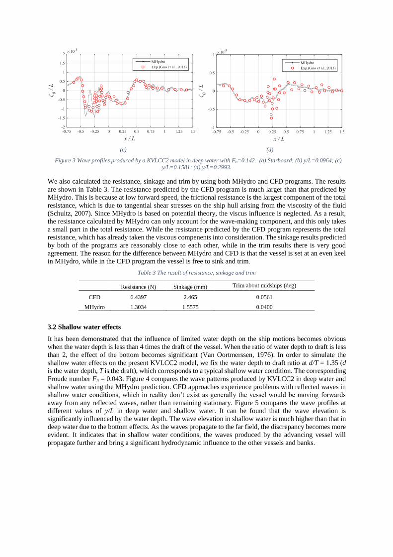
Figure 3 shows the wave profiles at different values of y/L. Generally, the agreement between the
measurements and the predictions from MHydro is very satisfactory. The wave profile predicted by the CFD
method is better than MHydro on the starboard side of the hull. However as discussed above, the downstream
profile predicted by the CFD approach is less satisfactory. Some spikes are observed in MHydro results on
the downstream side in Figure 3 (c), which corresponds to the divergent waves. These waves were also
predicted by Peng (2014). However, the measurements used here fail to capture these small amplitude waves.
At y/L = 0.2993, the amplitude of the divergent waves becomes very small. In order to obtain a better wave
elevation, a high quality free surface mesh is required. These fine meshes can guarantee that the waves will
not be damped before it propagates to the far field (Bunnik, 1999), but it will affect the computational time.
In the present study, we are aim to find the shallow water effects. Therefore, the panel number is restricted
in MHydro, in order to shorten the computational time. That is the reason why MHydro fails to predict the
fluctuations in the far field, as shown in Figure 3 (d). It can still be concluded that MHydro is a verified
numerical tool for predicting the wave patterns by a travelling vessel in deep water.
(d) (b)
Figure 2 Wave contour produced by a KVLCC2 model in deep water with Fn=0.142. (a) Comparison between MHydro (up
half) and CFD (lower half); (b) CFD results: up half of the figure is the wave pattern with the vessel static at even keel and
lower half of the figure is the wave pattern with the vessel free to sink and trim.
(a) (b)
X (m)
Y(m
)
-6 -4 -2 0 2 4
-3
-2
-1
0
1
2
3
0(m): -0.02 -0.016 -0.012 -0.008 -0.004 0 0.004 0.008 0.012 0.016 0.02
y / L = 0.1581
y / L = 0.2993
y / L = 0.0964
X (m)
Y(m
)
-6 -4 -2 0 2 4
-3
-2
-1
0
1
2
3
0(m): -0.02 -0.016 -0.012 -0.008 -0.004 0 0.004 0.008 0.012 0.016 0.02
y / L = 0.1581
y / L = 0.2993
y / L = 0.0964
MHydro
CFD
Free to trim and sink
Static
(c) (d)
Figure 3 Wave profiles produced by a KVLCC2 model in deep water with Fn=0.142. (a) Starboard; (b) y/L=0.0964; (c)
y/L=0.1581; (d) y/L=0.2993.
We also calculated the resistance, sinkage and trim by using both MHydro and CFD programs. The results
are shown in Table 3. The resistance predicted by the CFD program is much larger than that predicted by
MHydro. This is because at low forward speed, the frictional resistance is the largest component of the total
resistance, which is due to tangential shear stresses on the ship hull arising from the viscosity of the fluid
(Schultz, 2007). Since MHydro is based on potential theory, the viscus influence is neglected. As a result,
the resistance calculated by MHydro can only account for the wave-making component, and this only takes
a small part in the total resistance. While the resistance predicted by the CFD program represents the total
resistance, which has already taken the viscous compenents into consideration. The sinkage results predicted
by both of the programs are reasonably close to each other, while in the trim results there is very good
agreement. The reason for the difference between MHydro and CFD is that the vessel is set at an even keel
in MHydro, while in the CFD program the vessel is free to sink and trim.
Table 3 The result of resistance, sinkage and trim
Resistance (N) Sinkage (mm) Trim about midships (deg)
CFD 6.4397 2.465 0.0561
MHydro 1.3034 1.5575 0.0400
3.2 Shallow water effects
It has been demonstrated that the influence of limited water depth on the ship motions becomes obvious
when the water depth is less than 4 times the draft of the vessel. When the ratio of water depth to draft is less
than 2, the effect of the bottom becomes significant (Van Oortmerssen, 1976). In order to simulate the
shallow water effects on the present KVLCC2 model, we fix the water depth to draft ratio at d/T = 1.35 (d
is the water depth, T is the draft), which corresponds to a typical shallow water condition. The corresponding
Froude number Fn = 0.043. Figure 4 compares the wave patterns produced by KVLCC2 in deep water and
shallow water using the MHydro prediction. CFD approaches experience problems with reflected waves in
shallow water conditions, which in reality don’t exist as generally the vessel would be moving forwards
away from any reflected waves, rather than remaining stationary. Figure 5 compares the wave profiles at
different values of y/L in deep water and shallow water. It can be found that the wave elevation is
significantly influenced by the water depth. The wave elevation in shallow water is much higher than that in
deep water due to the bottom effects. As the waves propagate to the far field, the discrepancy becomes more
evident. It indicates that in shallow water conditions, the waves produced by the advancing vessel will
propagate further and bring a significant hydrodynamic influence to the other vessels and banks.

Figure 4 Wave contour produced by a KVLCC2 model at Fn=0.043. The upper half of the figure is the wave elevation at d/T
= 1.35. The lower half of the figure is the wave elevation at infinite water depth.
(a) (b)
(c) (d)
Figure 5 Wave profiles produced by a KVLCC2 model in shallow water (d / T = 1.35) with Fn= 0.043. (a) Starboard;
(b) y/L=0.0964; (c) y/L=0.1581; (d) y/L=0.2993.
In order to find the bottom effects on an advancing vessel, we calculate the wave-making resistance, as well
as the sinkage and trim at different water depths. The Froude number is 0.043, and d/T varies from 1.1 to 20.
The calculation results are shown in Figure 6. It can be observed that the water depth plays a critical role in
the hydrodynamic behaviour of an advancing vessel. Since the forward speed discussed here is very small,
the so-called depth Froude number is far beyond the critical value 1. It is very interesting to find that in the
extreme shallow water range, the wave-making resistance witnesses a sudden decrease. The peak resistance
can be observed at d/T = 1.35, and then as the water depth increases, the wave-making resistance drops
dramatically. But when d/T becomes larger than 10, the decreasing trend becomes very slow, which indicates
that it can be regarded as infinite water depth at d/T > 10. Similar observations can also be found in sinkage
and trim, as shown in Figure 6 (b) and Figure 6(c). As the water depth increases, the sinkage and trim drops
rapidly. At d/T > 5, the decreasing trend becomes very slow. It can be concluded from Figure 6 that in shallow water conditions, the hydrodynamic loads on the advancing vessels are very large compared to those
in deep water condition. The speed of the vessel must be restricted in order to avoid the squat or grounding.
X (m)
Y(m
)
-8 -6 -4 -2 0 2 4
-3
-2
-1
0
1
2
3
0(m): -1.0E-03 -6.0E-04 -2.0E-04 2.0E-04 6.0E-04 1.0E-03 1.4E-03
Deep water
Shallow water

(a) (b)
(c)
Figure 6 Results in different water depths. (a) Wave-making resistance; (b) sinkage; (c) trim.
4 Conclusions
The shallow water effects were discussed in the present paper. We calculated the hydrodynamic loads and
wave patterns of a KVLCC2 model travelling in deep water based on 3D Rankine source panel method. The
results from a commercial CFD program and experimental measurements were also included to verify our
in-house developed program MHydro. Very satisfactory agreement has been achieved in deep water. Then
the program was extended to predict the hydrodynamic performance of the advancing vessel in shallow
water. Numerical results showed that the wave elevation in shallow water was much higher than that in deep
water due to the bottom effects and the waves produced by the advancing vessel would propagate further
and could bring a significant hydrodynamic influence to other vessels and banks. It also showed that in
shallow water condition, the hydrodynamic loads on the advancing vessels were very large compared to
those in deep water condition. The speed of the vessel must be restricted in order to avoid the squat or
grounding in shallow water areas.
5 Acknowledgments
The work reported in this paper was performed within the project “Energy Efficient Safe Ship Operation
(SHOPERA)” funded by the European commission under contract No. 605221.
6 References
Andersen, P., 1979. Ship motions and sea loads in restricted water depth. Ocean Engineering 6, 557-569.
Bunnik, T., 1999. Seakeeping calculations for ships, taking into account the non-linear steady waves, PhD thesis.
Delft University of Technology, The Netherlands.
Guo, B.J., Deng, G.B., Steen, S., 2013. Verification and validation of numerical calculation of ship resistance and
flow field of a large tanker. Ships and Offshore Structures 8, 3-14.
Hess, J.L., Smith, A.M.O., 1964. Calculation of nonlifting potential flow about arbitrary three-dimensional bodies.
Journal of Ship Research 8, 22-44.
Kim, C.H., 1969. Hydrodynamic forces and moments for heaving swaying, and rolling cylinders on water of dinite
depth. Journal of Ship Research 13, 137-154.
Kim, W.J., Van, S.H., Kim, D.H., 2001. Measurement of flows around modern commercial ship models.
Experiments in Fluids 31, 567-578.

Lataire, E., Vantorre, M., Delefortrie, G., 2012. A prediction method for squat in restricted and unrestricted
rectangular fairways. Ocean Engineering 55, 71-80.
Newman, J.N., 1976. Linearized wave resistance, International Seminar on Wave resistance, Tokyo.
Peng, H., Ni, S., Qiu, W., 2014. Wave pattern and resistance prediction for ships of full form. Ocean Engineering
87, 162-173.
Prins, H.J., 1995. Time domain calculations of drift forces and moments, PhD Thesis. Delft University of
Technology, The Netherlands.
Schultz, M.P., 2007. Effects of coating roughness and biofouling on ship resistance and powering. Biofouling 23,
331-341.
Tuck, E.O., 1970. Ship motions in shallow water. Journal of Ship Research 14, 317-328.
Van Oortmerssen, G., 1976. The motions of a ship in shallow water. Ocean Engineering 3, 221–255.
Varyani, K.S., 2006. Squat effects on high speed craft in restricted waterways. Ocean Engineering 33, 365-381.
Yao, J.-x., Zou, Z.-j., 2010. Calculation of ship squat in restricted waterways by using a 3D panel method. Journal
of Hydrodynamics, Ser. B 22, 489-494.
Yuan, Z.M., Incecik, A., Day, A., 2014. Verification of a new radiation condition for two ships advancing in
waves. Applied Ocean Research 48, 186-201.


