Download - Numerical solution for an inverse MRI problem using a regularised boundary element method

ARTICLE IN PRESS
0955-7997/$ - se
doi:10.1016/j.en
�CorrespondE-mail addr
Engineering Analysis with Boundary Elements 32 (2008) 658–675
www.elsevier.com/locate/enganabound
Numerical solution for an inverse MRI problem using a regularisedboundary element method
Liviu Marina,�, Henry Powera, Richard W. Bowtellb, Clemente Cobos Sanchezb,Adib A. Beckera, Paul Gloverb, Arthur Jonesa
aSchool of Mechanical, Materials and Manufacturing Engineering, The University of Nottingham, University Park, Nottingham NG7 2RD, UKbSir Peter Mansfield Magnetic Resonance Centre, School of Physics and Astronomy, The University of Nottingham, Nottingham Park,
Nottingham NG7 2RD, UK
Received 16 June 2007; accepted 26 November 2007
Available online 14 March 2008
Abstract
We investigate the reconstruction of a divergence-free surface current distribution from knowledge of the magnetic flux density in a
prescribed region of interest in the framework of static electromagnetism. This inverse problem is motivated by the design of gradient
coils used in magnetic resonance imaging (MRI) and is formulated using its corresponding integral representation according to potential
theory. A constant boundary element method (BEM) which satisfies the continuity equation for the current density, i.e. divergence-free
BEM, and was originally proposed by Lemdiasov and Ludwig [A stream function method for gradient coil design. Concepts Magn
Reson B Magn Reson Eng 2005;26B:67–80], is presented based on geometrical arguments with respect to the linear (flat) triangular
boundary elements employed in order to emphasise its possible extension to further higher-order divergence-free interpolations. Since the
discretised BEM system is ill-posed and hence the associated least-squares solution may be inaccurate and/or physically meaningless, the
Tikhonov regularisation method is employed in order to retrieve accurate and physically correct solutions. A rigorous numerical
approximation for the calculation the magnetic energy, which reduces the errors induced by employing the approach of Lemdiasov and
Ludwig [A stream function method for gradient coil design. Concepts Magn Reson B Magn Reson Eng 2005;26B:67–80], is also
proposed.
r 2008 Elsevier Ltd. All rights reserved.
Keywords: Inverse problem; Regularisation; Divergence-free boundary element method (BEM); Magnetic resonance imaging (MRI); Electromagnetism;
Coil design
1. Introduction
Magnetic resonance imaging (MRI) is a non-invasivetechnique for imaging the human body, which hasrevolutionised the field of diagnostic medicine. MRI relieson the generation of highly controlled magnetic fields thatare essential to the process of image production. Inparticular, an extremely homogeneous, strong, static fieldis required to polarise the sample and provide a uniformfrequency of precession, while pure field gradients areneeded to encode the spatial origin of MR signals. The fieldgradients are generated by carefully arranged wire dis-
e front matter r 2008 Elsevier Ltd. All rights reserved.
ganabound.2007.11.015
ing author. Tel.: +44115 8467683; fax: +44 115 9513800.
ess: [email protected] (L. Marin).
tributions generally placed on surfaces surrounding theimaging subject known as gradient coils.Over the last two decades, many theoretical design
methods for the construction of MRI gradient coils havebeen developed. In one of the first papers on this subject,Bangert and Mansfield [1] produced a simple coil designthat generated a high gradient strength per unit currentwhilst providing a low coil inductance. The majority ofearly MRI systems employed gradient coils based onsimple saddle and loop units which are positioned so as tonull as many undesired terms in the spherical harmonicexpansion of the field at the coil centre, see e.g. Romeoand Hoult [2]. However, coils composed of discrete wireunits generally have high inductance at fixed gradientstrength and often have high length to diameter ratios.

ARTICLE IN PRESSL. Marin et al. / Engineering Analysis with Boundary Elements 32 (2008) 658–675 659
Improved performance can be achieved by using coilscomposed of distributed wirepaths which are spread moreuniformly over the coil surface. In order to generate suchdesigns, Turner [3] developed a Fourier–Bessel expansionof the magnetic field generated by currents flowing on thesurface of a cylinder. Inversion of the relationship betweenthe current density and the corresponding magnetic fieldallowed the design of gradient, solenoidal and shim coilscapable of generating a specified or target field. A methodfor designing coils with the minimum inductance consistentwith the field specification was also presented by Turner [4].Schweikert et al. [5] have used a Lagrange multiplierformalism to allow the magnetic field specified at discretelocations in space to be used as constraints in an explicitminimisation of the power dissipated by a coil. Minimumpower designs have also been proposed by Bowtell andMansfield [6]. These methods of coil design have beenimplemented using the fast Fourier transform to calculatematrix elements and evaluate the current densities. Themethod of conjugate gradient descent for the minimisationof the gap functional between the desired and calculatedmagnetic fields with respect to the current element positionhas been addressed by Wong et al. [7]. Carlson et al. [8]have developed an inductance minimisation techniquewhich automatically incorporates finite length, by initiallyexpanding the current density as a Fourier series. Themajority of gradient coil designs are based on a cylindricalgeometry in which the gradient wirepaths are confined tothe surface of a cylinder. It is also, however, possible todesign gradient coils using a variety of alternativegeometries including planar [9] and hemispherical forms[10]. Several generic gradient coil designs, as well ascomputational analysis approaches, were described in areview by Turner [11].
There are important studies in the literature that aredevoted to the design of gradient coils used in MRI basedon computational methods. Liu [12] has considered a bi-planar design and suggested a minimisation procedure forthe magnetic energy, which is proportional to the totalinductance, subject to the magnetic field being equal to adesired distribution in a specified region of interest. Greenet al. [13] have proposed an approach similar to Liu [12],namely the minimisation of a weighted combination ofpower, inductance and the squared difference between theactual and the desired fields. Leggett et al. [14] haveinvestigated multilayer transverse cylindrical coils byconsidering a cost function as a weighted combination ofinductance and power loss, and imposing the conditionthat the magnetic field equals certain values at specifiedpoints. Recently, Lemdiasov and Ludwig [15] havereported a new design approach for the construction ofgradient coils used in MRI by considering an integralrepresentation formula that satisfies the continuity equa-tion for the surface current density, constant interpolationand the minimisation of a constrained cost functionbetween the actual and the desired magnetic fields in aregion of interest.
The boundary element method (BEM) is a numericalmethod essentially based on the integral formulation of theproblem under consideration, see e.g. Brebbia et al. [16],and it is now a well established technique in computationalelectromagnetics and particularly in magnetostatics, seee.g. Adriaens et al. [17], Nicolet et al. [18], and Nicolet[19,20]. In this paper, we investigate the numericalreconstruction of a divergence-free surface current dis-tribution from knowledge of the magnetic flux density in aprescribed region of interest in the framework of staticelectromagnetism. This inverse problem is motivatedby the design of gradient coils used in MRI and isformulated using its corresponding integral representationaccording to potential theory. A constant BEM whichsatisfies the continuity equation for the current density, i.e.divergence-free BEM, and was originally proposed byLemdiasov and Ludwig [15], is presented based ongeometrical arguments with respect to the linear (flat)triangular boundary elements employed in order toemphasise its possible extension to further higher-orderdivergence-free interpolations. It should be mentionedthat, in classical BEM formulations of the inverse problemthat is analysed in this paper, the divergence-free conditionfor the current density has usually to be imposed in theform of additional constraints to the correspondingdiscretised BEM system of algebraic linear equations.However, in the present approach no additional con-straints are required for the current density to satisfythe continuity equation, as the interpolation functionsalready satisfy this condition. Since the discretised BEMsystem is ill-posed and its associated solution obtained viaa direct solver may be inaccurate and/or physicallymeaningless, regularisation methods are employed inorder to retrieve accurate and physically correct solutions.In our study, this is achieved by using the Tikhonovregularisation method, where the regularisation term isgiven by the norm related to the magnetic energy. Since theapproximation for the magnetic energy proposed byLemdiasov and Ludwig [15] is not appropriate forboundary elements close to one another and hence itinduces additional significant errors to the ill-posedproblem under investigation, a rigorous numerical approx-imation for the magnetic energy is also presented. Theefficiency of the proposed numerical method is illustratedby numerical examples for cylindrical and hemisphericalx- and z-gradient coil designs.
2. Mathematical formulation
In a non-magnetic material, such as biological tissue, the
magnetic induction field B ¼ ðBx;By;BzÞT satisfies the
following system of partial differential equations, see e.g.Jackson [21]:
r � BðxÞ ¼ m0JðxÞ; r � BðxÞ ¼ 0; x ¼ ðx; y; zÞ 2 R3.
(1)
ARTICLE IN PRESSL. Marin et al. / Engineering Analysis with Boundary Elements 32 (2008) 658–675660
Here m0 ¼ 4p� 10�7 N=A2 is the permeability of the free-space and J ¼ ðJx; Jy; JzÞ
T is the current density which isdefined as a surface current density Jcoil ¼ ðJcoil
x ; Jcoily ;
Jcoilz Þ
T, i.e.
JðxÞ ¼ Jcoilðx0Þdðx0; xÞ; x 2 R3; x0 2 Gcoil, (2)
where Gcoil � R3 is the coil surface and dðx0; xÞ is theKronecker delta function, such that
r � JcoilðxÞ ¼ 0; JcoilðxÞ � mðxÞ ¼ 0; x 2 Gcoil, (3)
with m the outward unit vector normal to the coil surface Gcoil.If the vector potential A ¼ ðAx;Ay;AzÞ
T is introduced as
BðxÞ ¼ r � AðxÞ; x 2 R3, (4)
then the system of partial differential equations (1) reducesto the following Poisson equation for the vector potential A:
r2AðxÞ ¼ m0JðxÞ; x 2 R3. (5)
In the direct problem formulation, the current density Jcoil
is known on the coil surface Gcoil, satisfies the divergence-free condition (31) and lies on the plane tangent to the coilsurface Gcoil, see Eq. (32), whilst the vector potential A isdetermined from the Poisson equation (5) by employing itsintegral representation, namely
AðxÞ ¼ m0
ZR3
u�ðx;x0ÞJðx0Þdx0
¼ m0
ZGcoil
u�ðx;x0ÞJcoilðx0ÞdGðx0Þ; x 2 R3, (6)
where u�ðx; x0Þ is the Green function for the 3D Laplaceequation given by
u�ðx;x0Þ ¼1
4pjx� x0j; x;x0 2 R3. (7)
On using Eqs. (4) and (6), the magnetic induction field maybe recast as
BðxÞ ¼ m0
ZGcoil
rxu�ðx;x0Þ � Jcoilðx0ÞdGðx0Þ; x 2 R3. (8)
Motivated by the design of gradient coils for use in MRI,we investigate the reconstruction of the divergence-freesurface current distribution Jcoil from knowledge of onecomponent of the magnetic flux density B, generally Bz, in aprescribed region of interest O � R3. More precisely, wefocus on the following inverse problem:
Given eBzðxÞ; x 2 O; find JcoilðxÞ; x 2 Gcoil,
such that
BzðxÞ ¼ eBzðxÞ; x 2 O; and r � JcoilðxÞ ¼ 0,
JcoilðxÞ � mðxÞ ¼ 0; x 2 Gcoil. (9)
3. Constant divergence-free BEM interpolation
In this section, we describe the approach of Lemdiasovand Ludwig [15] which is based on the integral representa-tion formula for the vector potential that satisfies the
continuity equation for the surface current density andemploys a constant approximation. Furthermore, we pre-sent the constant divergent-free interpolation for the currentdensity, Jcoil, which was originally introduced by Lemdiasovand Ludwig [15], based on geometrical arguments withrespect to the linear triangular boundary elements em-ployed, in order to emphasise its possible extension tofurther higher-order divergent-free approximations.
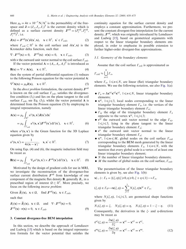
3.1. Geometry of the boundary elements
Assume that the coil surface Gcoil is approximated as
Gcoil �[Nn¼1
Gn,
where Gn, 1pnpN, are linear (flat) triangular boundaryelements. We use the following notation, see also Fig. 1(a):
�
Gn ¼ Dxn1xn2xn3, 1pnpN, linear triangular boundaryelements; � xnj , 1pjp3, local nodes corresponding to the lineartriangular boundary element Gn, i.e. the vertices of thelinear triangular boundary element Gn;
� Gnj the edge of the triangular boundary element Gnopposite to the vertex xnj, 1pjp3;
� mnj the outward unit vector normal to the edge Gnj ,1pjp3, lying in the plane tangent to the lineartriangular boundary element Gn;
� mn the outward unit vector normal to the lineartriangular boundary element Gn;
� xm, 1pmpM, global nodes on the coil surface Gcoilcorresponding to the BEM mesh generated by the lineartriangular boundary elements Gn, 1pnpN, with themention that every global node is a vertex of at least onelinear triangular boundary element;
� N the number of linear triangular boundary elements; � M the number of global nodes on the coil surface, Gcoil.The parametrisation of the linear triangular boundaryelements is given by, see also Fig. 1(b):
xð�; �Þ : G0 ¼ fðx; ZÞjxX0; ZX0; xþ Zp1g�!Gn,
ðx; ZÞ 2 G0 7�!xðx; ZÞ ¼X3j¼1
Njðx; ZÞxnj 2 Gn, (10)
where Njðx; ZÞ, 1pjp3, are geometrical shape functionsgiven by
N1ðx; ZÞ ¼ x; N2ðx; ZÞ ¼ Z; N3ðx; ZÞ ¼ 1� x� Z. (11)
Consequently, the derivatives in the x- and Z-directionsmay be recast as
snxðx; ZÞ ¼qxðx; ZÞ
qx¼ xn1 � xn3 ¼ snx,
snZðx; ZÞ ¼qxðx; ZÞ
qZ¼ xn2 � xn3 ¼ snZ. (12)

ARTICLE IN PRESS
Fig. 1. Schematic diagram of (a) the linear triangular boundary element, Gn, in the physical space R3, and (b) the transformed linear triangular boundary
element G0ðx; ZÞ in the parametric space ðx; ZÞ. (c) The set Cm of boundary elements Gn adjacent to the global node xm and the corresponding vector vn;iðm;nÞ
in the physical space R3.
L. Marin et al. / Engineering Analysis with Boundary Elements 32 (2008) 658–675 661
Then the surface metric (Jacobian) Jn and the outward unitvector mn normal to the linear triangular boundary elementGn are given by
Jnðx; ZÞ ¼ jsnxðx; ZÞ � snZðx; ZÞj ¼ jsnx � snZj ¼ Jn (13)
and
mnðx; ZÞ ¼1
Jnðx; ZÞsnxðx; ZÞ � snZðx; ZÞ ¼
1
Jn snx � snZ ¼ mn,
(14)
respectively.
3.2. Basis functions
On every linear triangular boundary element Gn, wedefine the following vectors, see also Figs. 1(a) and (b):
vn1ðx; ZÞ ¼ �1
Jnðx; ZÞsnZðx; ZÞ ¼
xn3 � xn2
Jn ¼ vn1;
vn2ðx; ZÞ ¼1
Jnðx; ZÞsnxðx; ZÞ ¼
xn1 � xn3
Jn ¼ vn2;
vn1ðx; ZÞ ¼ 1Jnðx;ZÞ ½�snxðx; ZÞ þ snZðx; ZÞ ¼
xn2 � xn1
Jn ¼ vn3:
8>>>>>>>><>>>>>>>>:(15)
From definition (15), it follows that, for every lineartriangular boundary element Gn, the vectors vnjðx; ZÞ ¼ vnj
satisfy the identity:X3j¼1
vnjðx; ZÞ ¼X3j¼1
vnj ¼ 0 for x ¼ xðx; ZÞ 2 Gn. (16)
Next, we define the incidence function i as follows:
ið�; �Þ : f1; 2; . . . ;Mg � f1; 2; . . . ;Ng�!f0; 1; 2; 3g,
ðm; nÞ7�!iðm; nÞ ¼0 if xmaxnj ; 8j 2 f1; 2; 3g;
j if 9j 2 f1; 2; 3g : xm ¼ xnj :
((17)
For every global node xm, 1pmpM, we define the setCm � Gcoil of linear triangular boundary elements Gn,1pnpN, adjacent to xm, see also Fig. 1(c), i.e.
Cm ¼[Nn¼1
iðm;nÞa0
Gn; 1pmpM. (18)
The vector basis function fm associated with the globalnode xm is defined by
fmð�Þ : Gcoil�!R3; fmðxÞ ¼vn;iðm;nÞ if x 2 Cm;
0 if xeCm
((19)

ARTICLE IN PRESSL. Marin et al. / Engineering Analysis with Boundary Elements 32 (2008) 658–675662
and clearly its support is a subset of Cm, i.e. supp fm ¼
fx 2 GcoiljfmðxÞa0g � Cm. It should be noted that the basis
function fm associated with the global node xm given byEq. (19) is piecewise constant, see also the definition (15) ofthe vectors vnj , 1pjp3, 1pnpN.
3.3. Surface current density
The current density Jcoil on the coil surface Gcoil is thenapproximated by
JcoilðxÞ �XMm¼1
ImfmðxÞ ¼
XMm¼1
Im
XN
n¼1iðm;nÞa0
vn;iðm;nÞ; x 2 Gcoil,
(20)
where Im 2 R, 1pmpM, are unknown coefficients thatcorrespond to the stream function intensities at each of theglobal nodes xm, 1pmpM. For direct problems, thestream function intensities are determined from appro-priate boundary conditions, while in the case of inverseproblems, they are obtained by solving a minimisationproblem.
From Eqs. (14) and (15) it follows that for everytriangular boundary element, Gn, the vectors v
njðx; ZÞ vnj ,1pjp3, and the outward unit normal vector mnðx; ZÞ mn
are orthogonal and hence expression (20) forces theapproximated current density Jcoil to lie in the planetangential to the coil surface, Gcoil, i.e. condition (32) issatisfied. Furthermore, the interpolation given by Eq. (20)is divergence-free pointwise, i.e. the divergence-free condi-tion (31) is satisfied, since r � vnj ¼ 0 for all 1pjp3 and1pnpN.
The unknown coefficients Im, 1pmpM, can also bedefined locally for every linear triangular boundary elementGn, 1pnpN, i.e.
Inj ¼ Imjwhere mj 2 f1; 2; . . . ;Mg : iðmj ; nÞ ¼ j. (21)
Consequently, we obtain the following constant diver-gence-free approximation for the surface current density onevery linear triangular boundary element Gn, 1pnpN:
JcoilðxÞ �X3j¼1
Inj vnj ¼
X3j¼1
Imjvn;iðmj ;nÞ; x 2 Gn. (22)
It should be noted that the degree of the approximation(20) for the surface current density Jcoil is one degree lessthan the degree of the triangular boundary elementsGn, 1pnpN, employed since the vectors vnjðx; ZÞ vnj ,1pjp3, are related to the derivatives of the geometricalshape functions Njðx; ZÞ, 1pjp3, associated with the lineartriangular boundary element Gn, see Eqs. (10)–(15).Consequently, higher-order interpolation formulae of anydegree k40 for the surface current density Jcoil can beeasily derived by considering the appropriate geometricalshape functions Njðx; ZÞ of degree ðk þ 1Þ, associated withthe triangular boundary element, Gn, but these are deferredto future work. It is important to note that the collocation
points, i.e. global nodes, are always located at the verticesof the triangular boundary elements employed in the BEMmeshing of the coil surface, Gcoil. Therefore, increasing thedegree of the interpolation for the surface current densitywill not affect the number of collocation points and thusthe dimension of the resulting BEM system of linearalgebraic equations.
3.4. Magnetic vector potential
According to Eqs. (8), (20) and (22), the magnetic vectorpotential A is approximated by
AðxÞ �m04p
XN
n¼1
ZGn
X3j¼1
Inj
vnj
jx� x0jdGðx0Þ
¼m04p
XMm¼1
Im
XN
n¼1iðm;nÞa0
ZGn
vn;iðm;nÞ
jx� x0jdGðx0Þ,
x 2 R3. (23)
Eq. (23) may be recast as
AðxÞ �XMm¼1
ImgmðxÞ; x 2 R3, (24)
where
gmðxÞ ¼m04p
XN
n¼1iðm;nÞa0
ZGn
vn;iðm;nÞ
jx� x0jdGðx0Þ; x 2 R3; 1pmpM.
(25)
3.5. Magnetic flux density
On using Eqs. (8), (20) and (22), we obtain the followingpiecewise constant approximation for the magnetic fluxdensity B:
BðxÞ �m04p
XN
n¼1
ZGn
X3j¼1
Inj
�ðx� x0Þ � vnj
jx� x0j3dGðx0Þ
¼m04p
XMm¼1
Im
XN
n¼1iðm;nÞa0
ZGn
�ðx� x0Þ � vn;iðm;nÞ
jx� x0j3dGðx0Þ,
x 2 R3. (26)
Eq. (26) may be expressed as
BðxÞ �XMm¼1
ImhmðxÞ; x 2 R3, (27)
where
hmðxÞ ¼m04p
XN
n¼1iðm;nÞa0
ZGn
�ðx� x0Þ � vn;iðm;nÞ
jx� x0j3dGðx0Þ,
x 2 R3; 1pmpM. (28)

ARTICLE IN PRESS
Fig. 2. The BEM mesh used for (a) the cylindrical, and (b) the
hemispherical coils, and the location of the internal points ð�Þ in the
corresponding spherical region of interest.
L. Marin et al. / Engineering Analysis with Boundary Elements 32 (2008) 658–675 663
4. Description of the algorithm
If the z-component of the magnetic flux density, B, isknown at L points in the region of interest O, as shown inFig. 2 for cylindrical and hemispherical coil surfaces, thenthe BEM discretisation of the inverse problem (9) yields thefollowing system of linear algebraic equations:
HI ¼ eBz. (29)
Here H 2 RL�M is the matrix containing the z-componentof the BEM vector hm given by Eq. (28) calculated at L
points in the region of interest O, eBz ¼ ðeB1z ; . . . ; eBL
z ÞT2 RL
is a vector containing the z-component of the magnetic fluxdensity at L points in the region of interest O and I 2 RM isa vector containing the unknown values of the streamfunction Im, 1pmpM, at the global nodes, i.e.
Hlm ¼ hmz ðx
lÞ
¼m04p
XN
n¼1iðm;nÞa0
ZGn
�ðxl � x0Þvn;iðm;nÞy þ ðyl � y0Þvn;iðm;nÞ
x
jxl � x0j3
�dGðx0Þ,
eBlz ¼ Bzðx
lÞ; 1plpL; 1pmpM. (30)
It is important to mention that the integrals involved inthe definition (30) of the components Hlm of the BEMmatrix H are non-singular since xleGcoil, 1plpL, andhence they can be evaluated numerically by employing aGauss quadrature for triangles, see e.g. Brebbia et al. [16].
4.1. Direct approach
A direct approach to solving the system of linearalgebraic equations (29) resulting from the discretisationof the present inverse problem can be implemented by, forexample, using the least-squares method. In this case, theleast-squares solution ILS to the inverse problem (9) issought as, see e.g. Tikhonov and Arsenin [22],
ILS 2 RM : FLSðILSÞ ¼ minI2RM
FLSðIÞ, (31)
where FLS is the least-squares functional defined by
FLS : RM�!½0;1Þ,
FLSðIÞ ¼1
2kHI� eBzk
2 ¼1
2
XL
l¼1
XMm¼1
HlmIm � eBlz
!2
. (32)
This minimisation problem is known to be equivalent tosolving the following system of normal equations:
HTHI ¼ HTeBz. (33)
However, the system of linear algebraic equations (29)cannot be solved by a direct approach, such as the least-squares method, since such a method would produce aninaccurate and/or physically meaningless solution due to thelarge value of the condition number of the system matrix H
which increases dramatically as the BEM mesh is refined.Several regularisation procedures have been developed tosolve such ill-conditioned systems, see for example Hansen[23]. In the following, we only consider the Tikhonovregularisation method and for further details on thismethod, we refer the reader to Tikhonov and Arsenin [22].
4.2. Magnetic energy and energy norm
The magnetic energy W defined by
W ¼1
2
ZGcoil
JcoilðxÞ � AðxÞdGðxÞ, (34)

ARTICLE IN PRESSL. Marin et al. / Engineering Analysis with Boundary Elements 32 (2008) 658–675664
can be approximated, according to Eqs. (20), (22) and(23), as
W �1
2
m04p
XN
m0¼1
XN
n0¼1
ZGm0
ZGn0
X3i¼1
X3j¼1
Im0i In0j
�vm0i � vn0j
jx� x0jdGðx0ÞdGðxÞ
¼1
2
m04p
XMm¼1
XMn¼1
ImIn
XN
m0¼1iðm;m0Þa0
XN
n0¼1iðn;n0Þa0
�
ZGm0
ZGn0
vm0;iðm;m0Þ � vn0 ;iðn;n0Þ
jx� x0jdGðx0ÞdGðxÞ. (35)
Eq. (35) may be recast as
W �1
2
XMm¼1
XMn¼1
LmnInIm, (36)
where the components of the inductance matrix L ¼
½Lmn 2 RM�M are given by
Lmn ¼m04p
�XN
m0¼1iðm;m0Þa0
XN
n0¼1iðn;n0Þa0
ZGm0
ZGn0
vm0;iðm;m0Þ � vn0;iðn;n0Þ
jx� x0j
�dGðx0ÞdGðxÞ; 1pm; npM. (37)
It should be mentioned that the inductance matrix L issymmetric, i.e.
Lmn ¼ Lmn; 1pm; npM. (38)
Furthermore, it can be shown numerically that theinductance matrix L is also positive definite, i.e.
PMm¼1
PMn¼1
LmnInImX0; 8I1; I2; . . . ; IM 2 R;
PMm¼1
PMn¼1
LmnInIm ¼ 0 () I1 ¼ I2 ¼ � � � ¼ IM ¼ 0:
8>>><>>>: (39)
The purpose of the regularisation techniques is tointroduce a smoothing norm and this is strongly related tothe magnetic energy W defined by Eq. (34). It should benoted that, since the inductance matrix L is symmetric andpositive definite, see Eqs. (38) and (39), the existence of the
square root matrix eL 2 RM�M associated with L, i.e.eL2 ¼ L, is ensured. Moreover, eL is also a symmetric matrix,
i.e. eLT ¼ eL. Consequently, the approximated magneticenergy W given by Eq. (36) is a quadratic and positivedefinite form which induces the following energy norm:
kIk2W ¼ keLIk2 ¼XM
m¼1
XMn¼1
LmnInIm ¼ 2W . (40)
4.3. Regularisation
The Tikhonov regularised solution Il to the inverseproblem (9) is sought as, see e.g. Tikhonov and Arsenin[22],
Il 2 RM : FlðIlÞ ¼ minI2RM
FlðIÞ, (41)
where Fl is the Tikhonov functional given by
Flð�Þ : RM�!½0;1Þ,
FlðIÞ ¼FLSðIÞ þ lW ¼1
2kHI� eBzk
2 þ1
2lkIk2W
¼1
2kHI� eBzk
2 þ1
2lkeLIk2
¼1
2
XL
l¼1
XMm¼1
HlmIm � eBlz
!2
þ1
2lXMm¼1
XMn¼1
LmnInIm, (42)
with l40 the regularisation parameter to be chosen.Formally, the Tikhonov regularised solution Il of theminimisation problem (41) is given by the solution of theregularised normal system of equations
ðHTHþ leLTeLÞIl ¼ HTeBz, (43)
that is
Il ¼ ðHTHþ leLTeLÞ�1HTeBz. (44)
Regularisation is necessary when solving ill-conditionedsystems of linear equations because the simple least-squaressolution, i.e. l ¼ 0, is completely dominated by contribu-tions from rounding errors. By adding regularisation weare able to damp out these contributions and ensure thatthe energy norm kIkW ¼ k
eLIk has a reasonable size. If toomuch regularisation, or damping, i.e. l is large, is imposedon the solution then it will not fit the given data eBz properlyand the residual norm kHI� eBzk will be too large. If toolittle regularisation is imposed on the solution, i.e. l issmall, then the fit will be good, but the solution will bedominated by the contributions from computationalerrors, and hence the energy norm kIkW ¼ k
eLIk will betoo large. To summarise, the Tikhonov regularisationmethod solves a minimisation problem using a smoothnessconstraint in order to provide a stable solution which fitsthe data and also has a minimum structure.
5. Numerical evaluation of the inductance matrix
Consider the double integral involved in the definition(37) of the components Lmn of the inductance matrix L,namely
Lm0n0 ¼
ZGm0
ZGn0
vm0;iðm;m0Þ � vn0;iðn;n0Þ
jx� x0jdGðx0ÞdGðxÞ,
1pm0; n0pN. (45)
ARTICLE IN PRESSL. Marin et al. / Engineering Analysis with Boundary Elements 32 (2008) 658–675 665
In the case of linear triangular boundary elements, i.e.constant interpolation for the current density, on usingEqs. (10)–(20), the double integral Lm0n0 defined byEq. (45) reduces to
Lm0n0 ¼ ðJm0vm0;iðm;m0ÞÞ � ðJn0vn0 ;iðn;n0ÞÞ
�
ZG0
ZG0
1
jxðx; ZÞ � x0ðx0; Z0Þjdðx0; Z0Þ
!|fflfflfflfflfflfflfflfflfflfflfflfflfflfflfflfflfflfflfflfflfflfflfflfflfflfflfflfflfflfflffl{zfflfflfflfflfflfflfflfflfflfflfflfflfflfflfflfflfflfflfflfflfflfflfflfflfflfflfflfflfflfflffl}
¼eLm0n0 ðx;ZÞ
dðx; ZÞ.
(46)
The evaluation of the double integral Lm0n0 given byEq. (45) or (46) requires special attention since a simpleapproximation of this integral was used by Lemdiasovand Ludwig [15]. More precisely, in the case of lineartriangular boundary elements, Lemdiasov and Ludwig [15]have approximated the denominator of the integrand bythe distance between the centres of mass of the lineartriangular elements Gm0 and Gn0 , respectively, and hencethey reduced the computation of the double integral tocalculating the surface area of the linear (flat) triangularelements Gm0 and Gn0 . Although this approximation mightbe suitable for elements located far from one another, itbecomes inappropriate for close triangular elements. It isimportant to mention that, in addition to the ill-posednessof the inverse problem investigated, such an approachinduces a significant numerical error and this will affect theaccuracy of the solution.
In this study, the double integral Lm0n0 given by Eq. (45)or (46) is calculated numerically for the non-singular case,i.e. Gm0aGn0 and distðGn0 ;Gm0 Þa0, by employing the 2DGauss quadrature for triangles twice, see e.g. Brebbia et al.[16]. However, the integral fLm0n0 ðx; ZÞ defined in Eq. (46)involves the integration of a singular function for Gn0 ¼ Gm0 .Moreover, for Gn0aGm0 such that distðGn0 ;Gm0 Þ ¼ 0, theintegral fLm0n0 ðx; ZÞ is not singular, but a direct Gaussquadrature for triangles applied to it produces in generalinaccurate results. In order to overcome this situation, wetransform the integration of fLm0n0 ðx; ZÞ over G0 ¼ G0ðx
0; Z0Þinto an integration with respect to a local polar coordinatesystem ðr; yÞ centred at ðx00; Z
00Þ in the plane ðx0; Z0Þ of the
triangle G0, namely
ðr; yÞ7�!x0
Z0
!ðr; yÞ ¼
x00
Z00
!þ r
cos y
sin y
!,
0prprmaxðyÞ; yminpypymax. (47)
Here rmaxðyÞ is the upper bound for the polar distance, r,ymin and ymax are the lower and upper bounds, respectively,for the polar angle, y, and ðx00; Z
00Þ is the origin of the
local polar coordinate system. It should be noted that,by applying transformation (47), the singularity of theintegrand of fLm0n0 ðx; ZÞ is cancelled by the Jacobian,Jðr; yÞ ¼ r, of the transformation (47).
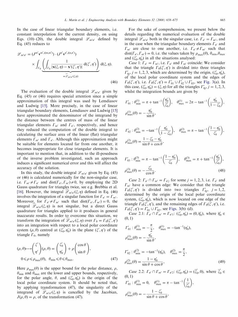
For the sake of comprehension, we present below thedetails regarding the numerical evaluation of the doubleintegral Lm0n0 both in the singular case, i.e. Gn0 ¼ Gm0 , andin the case when the triangular boundary elements Gn0 andGm0 are close to one another, i.e. Gn0aGm0 such thatdistðGn0 ;Gm0 Þ ¼ 0, i.e. the values taken by rmaxðyÞ, ymin,ymax
and ðx00; Z00Þ in all the situations analysed:
Case 1: Gn0 ¼ Gm0 , i.e. Gn0 and Gm0 coincide: We considerthat the triangle G0ðx
0; Z0Þ is divided into three trianglesG00j, j ¼ 1; 2; 3, which are determined by the origin, ðx00; Z
00Þ,
of the local polar coordinate system and the edges ofG0ðx
0; Z0Þ, i.e. G0ðx0; Z0Þ ¼ G001 [ G
002 [ G
003, see Fig. 3(a). In
this case, ðx00; Z00Þ ¼ ðx; ZÞ for all the triangles G
00j , j ¼ 1; 2; 3,
whilst the integration bounds are given by
G001 : yð1Þmin ¼ pþ tan�1
Z00x00
� �; yð1Þmax ¼ 2p� tan�1
Z001� x00
� �,
rð1ÞmaxðyÞ ¼ �Z00sin y
,
G002 : yð2Þmin ¼ �tan
�1 Z001� x00
� �; yð2Þmax ¼ p� tan�1
1� Z00x00
� �,
rð2ÞmaxðyÞ ¼1� x00 � Z00sin yþ cos y
,
G003 : yð3Þmin ¼ p� tan�1
1� Z00x00
� �; yð3Þmax ¼ pþ tan�1
Z00x00
� �,
rð3ÞmaxðyÞ ¼ �x00
cos y. (48)
Case 2: Gn0 \ Gm0 ¼ Gn0j for some j ¼ 1; 2; 3, i.e. Gn0 andGm0 have a common edge: We consider that the triangleG0ðx
0; Z0Þ is divided into two triangles G00j, j ¼ 1; 2,determined by the origin of the local polar coordinatesystem, ðx00; Z
00Þ, which is now located on one edge of the
triangle G0ðx0; Z0Þ, and the remaining edges of G0ðx
0; Z0Þ, i.e.G0ðx
0; Z0Þ ¼ G001 [ G002, see Figs. 3(b)–(d).
Case 2.1: Gn0 \ Gm0 ¼ Gn01: ðx00; Z00Þ ¼ ð0; Z
00Þ, where Z00 2
ð0; 1Þ
G001 : yð1Þmin ¼ �
p2; yð1Þmax ¼ �tan
�1ðZ00Þ,
rð1ÞmaxðyÞ ¼ �Z00sin y
,
G002 : yð2Þmin ¼ �tan
�1ðZ00Þ; yð2Þmax ¼p2,
rð2ÞmaxðyÞ ¼1� Z00
sin yþ cos y, (49)
Case 2.2: Gn0 \ Gm0 ¼ Gn02: ðx00; Z00Þ ¼ ðx
0
0; 0Þ, where x0
0 2
ð0; 1Þ
G001 : yð1Þmin ¼ 0; yð1Þmax ¼ p� tan�1
1
x00
� �,
rð1ÞmaxðyÞ ¼ �1� x00
sin yþ cos y,

ARTICLE IN PRESS
Fig. 3. Schematic diagram of the triangle G0ðx0; Z0Þ and the local polar coordinate system ðr; yÞ centred at ðx00; Z00Þ, used for the numerical integration of the
elements of the inductance matrix in (a) Case 1, (b) Case 2.1, (c) Case 2.2, (d) Case 2.3, and (e) Case 3.1, respectively.
L. Marin et al. / Engineering Analysis with Boundary Elements 32 (2008) 658–675666
G002 : yð2Þmin ¼ p� tan�1
1
x00
� �; yð2Þmax ¼ p,
rð2ÞmaxðyÞ ¼ �x00
cos y, (50)
Case 2.3: Gn0 \ Gm0 ¼ Gn03: ðx00; Z00Þ ¼ ðx
0
0; 1� x0
0Þ, wherex0
0 2 ð0; 1Þ
G001 : yð1Þmin ¼
3p4; yð1Þmax ¼ pþ tan�1
Z00x00
� �,
rð1ÞmaxðyÞ ¼ �x00
cos y,
G002 : yð2Þmin ¼ pþ tan�1
Z00x00
� �; yð2Þmax ¼
7p4,
rð2ÞmaxðyÞ ¼ �Z00sin y
. (51)
Case 3: Gn0 \ Gm0 ¼ fxn0jg for some j ¼ 1; 2; 3, i.e. Gn0 and
Gm0 have a common vertex, see Fig. 3(e).

ARTICLE IN PRESSL. Marin et al. / Engineering Analysis with Boundary Elements 32 (2008) 658–675 667
Case 3.1: Gn0 \ Gm0 ¼ fxn01g: ðx00; Z
00Þ ¼ ð1; 0Þ
G001 G0ðx0; Z0Þ : yð1Þmin ¼
3p4; yð1Þmax ¼ p; rð1ÞmaxðyÞ ¼ �
1
cos y,
(52)
Case 3.2: Gn0 \ Gm0 ¼ fxn02g: ðx00; Z
00Þ ¼ ð0; 1Þ
G001 G0ðx0; Z0Þ : yð1Þmin ¼ �
p2; yð1Þmax ¼ �
p4,
rð1ÞmaxðyÞ ¼ �1
sin y, (53)
Case 3.3: Gn0 \ Gm0 ¼ fxn03g: ðx00; Z
00Þ ¼ ð0; 0Þ
G001 G0ðx0; Z0Þ : yð1Þmin ¼ 0; yð1Þmax ¼
p2,
rð1ÞmaxðyÞ ¼1
sin yþ cos y. (54)
Hence for each of the cases presented above, the innerintegral fLm0n0 ðx; ZÞ may be recast as
fLm0n0 ðx; ZÞ
¼XJ0j¼1
Z yðjÞmax
yðjÞmin
Z rðjÞmaxðyÞ
rðjÞminðyÞ
rjxðx; ZÞ � x0½x0ðx00; Z
00; r; yÞ; Z
0ðx00; Z00;r; yÞj
dr
!dy,
(55)
where
G0ðx0; Z0Þ ¼
[J0j¼1
G00j and J0 2 f1; 2; 3g
depending upon the number of triangles G00j in whichtriangle G0ðx
0; Z0Þ is decomposed according to Cases 1–3.Therefore, in order to calculate numerically the doubleintegral Lm0n0 given by Eq. (45) or (46), the outer integralis evaluated numerically using the 2D Gauss quadra-ture for triangles, whilst for the inner integral fLm0n0 ðx; ZÞthe singularity is removed by introducing suitable localpolar coordinates and then applying twice the 1DGauss–Legendre quadrature for Eq. (55), see e.g. Brebbiaet al. [16].
6. Numerical results
In this section, we illustrate the results obtained usingthe numerical method described in Section 4 combinedwith the divergence-free BEM and the numerical integra-tion for the inductance matrix presented in Sections 3and 5, respectively. In addition, we investigate theconvergence and accuracy of the proposed numericalmethod, present a comparison between the numericalresults retrieved using the present method and thoseobtained by Lemdiasov and Ludwig [15], and also performa sensitivity analysis with respect to the choice of theregularisation parameter.
6.1. Examples
In order to demonstrate the performance of theproposed method, we solve the inverse problem (9) forthe following geometries, see also Figs. 2(a) and (b):
Example 1. Consider a cylindrical coil Gcoil ¼ fx ¼
ðx; y; zÞ 2 R3jx2 þ y2 ¼ R2;�hpzphg, where R ¼ 0:5mand h ¼ 1:0m, while the region of interest is a spherecentred at the origin of the coordinate system, i.e.O ¼ fx ¼ ðx; y; zÞ 2 R3jx2 þ y2 þ z2pr2g, where r ¼ 0:2m.
Example 2. Consider a hemispherical coil Gcoil ¼ fx ¼
ðx; y; zÞ 2 R3jx2 þ y2 þ z2 ¼ R2; zX0g, where R ¼ 0:175m.Here the region of interest is a sphere centred atxc ¼ ðxc; yc; zcÞ ¼ ð0; 0; 0:081Þ, i.e. O ¼ fx ¼ ðx; y; zÞ 2R3jðx� xcÞ
2þ ðy� ycÞ
2þ ðz� zcÞ2pr2g, where r ¼ 0:065m.
Since the geometries of the two types of coil considered inthis paper are symmetrical with respect to the z-axis, it is suffi-cient to investigate only the design of x- and z-gradients, i.e.eBzðxÞ ¼ Gxx; x 2 O and eBzðxÞ ¼ Gzz; x 2 O, (56)
where Gx 2 R and Gz 2 R are given. Although not presentedherein, it is reported that the numerical results obtained forthe cylindrical and hemispherical y-gradient coils are similarto those retrieved for the corresponding x-gradient coils, butrotated by an angle y ¼ p=2 about the z-axis. For the presentcomputations, we have considered Gx ¼ Gz ¼ 1:0Tm�1.The numerical results presented in this section have
been obtained using three different BEM meshes forthe coil surface, Gcoil, namely N 2 f1152; 2048; 3200gand N 2 f1128; 1888; 2840g linear triangular boundaryelements for the cylindrical and hemispherical coils,respectively. It should be noted that the aforementionedBEM meshes correspond to M 2 f600; 1056; 1640g andM 2 f577; 961; 1441g global nodes on the cylindricaland hemispherical coil surfaces, respectively, used forthe approximation of the unknown stream functionI ¼ ðI1; I2; . . . ; IMÞ
T. Moreover, for both coil geometriesanalysed in this study, the z-component of the magneticflux density is specified at L ¼ 351 internal points in thecorresponding spherical region of interest.
6.2. Reduction of the regularised system of normal equations
It is important to mention that the dimension of theregularised system of normal equations (43) can bedecreased for the coil surfaces analysed in this paper dueto the fact that these are not closed surfaces and there is nocurrent flux flowing into or out of the coil surface. Moreprecisely, the cylindrical and hemispherical coil surfacesconsidered are bounded by the following 3D curves:
Example 1. Cylindrical coil (R ¼ 0:5m and h ¼ 1:0m):
qGcoil ¼ gð1Þcoil [ gð2Þcoil:
gð1Þcoil ¼ fx ¼ ðx; y; zÞ 2 R3jx2 þ y2 ¼ R2; z ¼ �hg,
gð2Þcoil ¼ fx ¼ ðx; y; zÞ 2 R3jx2 þ y2 ¼ R2; z ¼ hg. (57)

ARTICLE IN PRESSL. Marin et al. / Engineering Analysis with Boundary Elements 32 (2008) 658–675668
Example 2. Hemispherical coil ðR ¼ 0:175mÞ:
qGcoil ¼ gð1Þcoil:
gð1Þcoil ¼ fx ¼ ðx; y; zÞ 2 R3jx2 þ y2 ¼ R2; z ¼ 0g. (58)
In order to derive the discrete condition for the streamfunction associated with the global nodes that belong to acurve bounding the coil surface, i.e. gðjÞcoil � qGcoil, weconsider a triangular boundary element Gn ¼ 4x
n1xn2xn3 �
Gcoil and, without any loss of the generality, assume thatGn \ g
ðjÞcoil ¼ fx
n2;xn3g, see Fig. 1. On considering mn1 theoutward unit vector normal to the edge Gn1 opposite tothe local node xn1 and lying in the plane tangent tothe triangular boundary element Gn, see also Fig. 1, weobtain
0 ¼ JcoilðxÞjGn1� mn1ðxÞ � ½In1v
n1ðxÞ
þ In2vn2ðxÞ þ In3v
n3ðxÞ � mn1ðxÞ
¼ ½In1vn1ðxÞ þ In2 ðv
n1ðxÞ þ vn2ðxÞ þ vn3ðxÞÞ|fflfflfflfflfflfflfflfflfflfflfflfflfflfflfflfflfflfflfflfflffl{zfflfflfflfflfflfflfflfflfflfflfflfflfflfflfflfflfflfflfflfflffl}¼0 according to Eq: ð16Þ
� In2ðvn1ðxÞ þ vn3ðxÞÞ þ In3v
n3ðxÞ � mn1ðxÞ
¼ ðIn1 � In2Þ ½vn1ðxÞ � mn1ðxÞ|fflfflfflfflfflfflfflfflfflfflffl{zfflfflfflfflfflfflfflfflfflfflffl}¼0 by definition
þðIn3 � In2Þ½vn3ðxÞ � mn1ðxÞ
¼ ðIn3 � In2Þ½vn3ðxÞ � mn1ðxÞ. (59)
Since vn3ðxÞ � mn1ðxÞa0, from Eq. (59) it follows that
In2 ¼ In3. (60)
By extending this rationale to all the triangularboundary elements that share two nodes with the curvegðjÞcoil � qGcoil, we obtain the discrete condition for thestream function associated with the global nodes thatbelong to a curve bounding the coil surface, namely
Im1¼ Im2
¼ � � � ¼ Imj; xm1 ;xm2 ; . . . ;xmj 2 gðjÞcoil. (61)
Consequently, if the coil surface Gcoil under considerationis bounded by the 3D curves gðjÞcoil, 1pjpJ, such that mj
global nodes are located on each curve gðjÞcoil, 1pjpJ, thenthe original dimension M of the regularised system ofnormal equations (43) is reduced to
eM ¼M �XJ
j¼1
ðmj � 1Þ.
It is worth mentioning that the dimensions of the matricesH and L involved in the original regularised system ofnormal equation (43), as well as the unknown streamfunction vector I, should be reduced accordingly.
6.3. Selection of the optimal regularisation parameter
The choice of the regularisation parameter, l, in theminimisation process of the Tikhonov functional (42) iscrucial for obtaining a stable, accurate and physicallycorrect numerical solution Il and this issue was notaddressed in a rigorous manner by Lemdiasov and Ludwig
[15]. As mentioned in Section 4.3, the optimal value lopt ofthe regularisation parameter, l, should be chosen such thata trade-off between the two quantities kHI� eBzk andkIkW ¼ k
eLIk involved in the minimisation of the func-tional (42) is attained.To achieve this, we introduce a term that characterises
the difference between the computed and desiredz-components of the magnetic flux density in the regionof interest, i.e. the relative percentage error defined by
errðBzðxÞ; lÞ ¼jBl
zðxÞ �eBzðxÞj
jeBzðxÞj� 100; x 2 O, (62)
where BlzðxÞ is the numerical z-component of the magnetic
flux density calculated at the point x in the regionof interest O, for a given regularisation parameter l,by employing the BEM-based algorithm described inSection 4. Furthermore, we define a global measure forthe percentage relative error errðBzðxÞ; lÞ given by Eq. (62)in the region of interest O, namely the maximum relativepercentage error
ErrðBz; lÞ ¼ maxx2O
errðBzðxÞ; lÞ. (63)
On assuming that a deviation �40 from the desiredz-component of the magnetic flux density eBz is admissiblein the region of interest O, such thateB�
zðxÞ ¼eBzðxÞð1� �Þ; x 2 O, (64)
then the choice of the optimal regularisation parameter loptis made by employing the maximum relative percentageerror given by Eq. (63) and the admissible level of variationin BzjO defined by relation (64), namely
lopt ¼ maxfl40jErrðBz; lÞp�g. (65)
Figs. 4(a) and (b) illustrate the maximum relativepercentage error ErrðBz; lÞ, as a function of the regularisa-tion parameter l, obtained using linear triangular bound-ary elements, for the cylindrical x- and z-gradient coils,respectively. It can be seen from these figures that the errorErrðBz; lÞ decreases as the regularisation parameter l tendsto zero. The optimal value of the regularisation parameter,chosen according to Eq. (65) and corresponding to adeviation of � ¼ 5% from the linearity of the x- andz-gradients, is given by lopt � 4:0� 10�9 and lopt � 3:0�10�8 in the case of the cylindrical x- and z-gradient coils,respectively. Although not presented herein, it is reportedthat a similar evolution of the error ErrðBz; lÞ with respectto the regularisation parameter l has been obtained for thehemispherical x- and z-gradient coils when using lineartriangular boundary elements.
6.4. Comparison with the results obtained by Lemdiasov and
Ludwig [15]
The numerical solution Il of the regularised system ofnormal equations (43), with l ¼ lopt given by Eq. (65),provides only a discrete distribution of the stream function

ARTICLE IN PRESS
10-12 10-10 10-8 10-6 10-4 10-2
Regularization parameter λ
0
20
40
60
80
100
Err
or E
rr (B
z; λ)
10-12 10-10 10-8 10-6 10-4 10-2
Regularization parameter λ
0
20
40
60
80
100
Err
or E
rr (B
z; λ)
Fig. 4. The maximum relative percentage error ErrðBz; lÞ, as a function of
the regularisation parameter l, obtained using N ¼ 3200 linear triangular
boundary elements, for the cylindrical (a) x-, and (b) z-gradient coils,
respectively.
−2 −1 0 1 2 3−1
−0.8
−0.6
−0.4
−0.2
0
0.2
0.4
0.6
0.8
1
θ
z
−2 −1 0 1 2 3−1
−0.8
−0.6
−0.4
−0.2
0
0.2
0.4
0.6
0.8
1
θ
z
Fig. 5. The contours of the stream function corresponding to the
cylindrical (a) x-, and (b) z-gradient coils given by Example 1, obtained
using the present method (—) and that of Lemdiasov and Ludwig [15]
(– –), respectively, with the optimal regularisation parameter lopt chosenaccording to Eq. (65), L ¼ 351 internal points in the region of interest and
N ¼ 3200 linear triangular boundary elements.
L. Marin et al. / Engineering Analysis with Boundary Elements 32 (2008) 658–675 669
at the global nodes of the BEM mesh employed. However,these discrete values should be extended to a continuousdistribution of the numerical stream function over theentire coil surface, Gcoil, and this is achieved by employingthe contours of the stream function using its discretedistribution and the Matlab (The Mathworks, Inc., Natick,MD, USA) contouring function. Hence, in the following,the numerically retrieved solutions of the inverse problemgiven by Eq. (9) are presented in terms of the contours ofthe stream function as described above.
Figs. 5(a) and (b) present the 2D contours of the streamfunction in the y2z plane corresponding to the cylindrical
x- and z-gradient coils, respectively, obtained using thepresent method and the approach of Lemdiasov andLudwig [15], respectively, with the optimal regularisationparameter lopt given by Eq. (65), L ¼ 351 internal points inthe region of interest and N ¼ 3200 linear triangularboundary elements. Here z 2 ½�1; 1 and y 2 ð�p;p arethe height and azimuthal cylindrical coordinates, respec-tively. It can be seen from these figures that, for bothcylindrical gradient coils considered, the contours of thestream function retrieved using the numerical methoddescribed in Section 4 combined with the divergence-freeBEM and the numerical integration for the inductancematrix presented in Sections 3 and 5, respectively, aredifferent from those corresponding to the approach ofLemdiasov and Ludwig [15]. This is a direct consequence of

ARTICLE IN PRESS
0 1 2 3 4 5 6
0.1
0.2
0.3
0.4
0.5
0.6
0.7
0.8
0.9
θ
cos
φ
0 1 2 3 4 5 6
0.1
0.2
0.3
0.4
0.5
0.6
0.7
0.8
0.9
θ
cos
φ
Fig. 6. The contours of the stream function corresponding to the
hemispherical (a) x- and (b) z-gradient coils given by Example 2, obtained
using the present method (—) and that of Lemdiasov and Ludwig [15]
(– –), respectively, with the optimal regularisation parameter lopt chosenaccording to Eq. (65), L ¼ 351 internal points in the region of interest and
N ¼ 2840 linear triangular boundary elements.
L. Marin et al. / Engineering Analysis with Boundary Elements 32 (2008) 658–675670
the approximation employed in this paper for computingnumerically the components of the inductance matrix L,see Section 5. It should be mentioned that, unlikethe coarse approximation proposed by Lemdiasov andLudwig [15], the present numerical approximation alle-viates significantly the error in the numerical evaluation ofthe inductance matrix and, consequently, the magneticenergy norm, and this is reflected by the different numericalresults obtained for the inverse problem investigated in thisstudy.
A similar conclusion can be drawn from Figs. 6(a)and (b) which illustrate the numerical results for thestream function in the y� cosf plane corresponding tothe hemispherical x- and z-gradient coils, respectively,obtained using the present method and the approach ofLemdiasov and Ludwig [15], with l ¼ lopt chosen accord-ing to Eq. (65), L ¼ 351 internal points in the region ofinterest and N ¼ 2840 linear triangular boundary elements.Here y 2 ½0; 2pÞ and f 2 ½0; p=2 are the azimuthal andcolatitude spherical coordinates, respectively. It should benoted that, in the case of the hemispherical coil, the so-called Lambert cylindrical equal-area projection, i.e. they� cosf plane, has been used to represent the 2D contoursof the stream function.
6.5. Influence of the regularisation parameter
It is interesting to investigate how the Tikhonovregularisation functional presented in Section 4.3 improvesthe accuracy of the numerical results, as well as theimportance of an appropriate criterion for choosing theoptimal regularisation parameter. To do so, we considerthe cylindrical x-gradient and the hemispherical z-gradientcoils only.
Figs. 7(a)–(c) show the 2D contours of the streamfunction in the z2y plane, obtained using N ¼ 3200 lineartriangular boundary elements, i.e. M ¼ 1640 globalnodes, L ¼ 351 internal points in the region of interestand various values of the regularisation parameter,namely l ¼ 1:0� 10�24lopt, l ¼ 4:0� 10�9 � lopt, andl ¼ 1:0� 10�11olopt, respectively, for the cylindricalx-gradient coil given by Example 1. From Figs. 7(a) and(b), it can be seen that the numerical solution Ilcorresponding to a large value of the regularisationparameter, i.e. l4lopt, yields contours of the streamfunction with a low energy norm, but which do not fitthe desired z-component of the magnetic flux density in theregion of interest. In contrast, the numerical solution Ilassociated with a very small value of the regularisationparameter, i.e. lolopt, yields contours of the streamfunction with an oscillatory behaviour, i.e. the correspond-ing energy norm is high, although the fit with the desired z-component of the magnetic flux density in the region ofinterest is very good, see Figs. 7(b) and (c).
A similar conclusion can be drawn from Figs. 8(a)–(c)which illustrate the 2D contours of the stream function inthe y� cosf plane, obtained using N ¼ 2840 linear
triangular boundary elements, i.e. M ¼ 1441 globalnodes, L ¼ 351 internal points in the region of interestand various values of the regularisation parameter,namely l ¼ 1:0� 10�24lopt, l ¼ 7:0� 10�9 � lopt, andl ¼ 1:0� 10�11olopt, respectively, for the hemisphericalz-gradient coil given by Example 2.
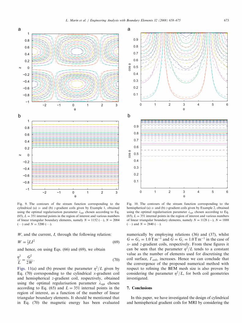
6.6. Convergence of the method
The convergence of the proposed numerical methodwith respect to refining the BEM mesh size is illustrated inFigs. 9(a) and (b) which represent the contours of the streamfunction corresponding to the cylindrical x- and z-gradientcoils, respectively, obtained using the optimal regularisa-

ARTICLE IN PRESS
−2 −1 0 1 2 3−1
−0.8
−0.6
−0.4
−0.2
0
0.2
0.4
0.6
0.8
1
θ
z
−2 −1 0 1 2 3−1
−0.8
−0.6
−0.4
−0.2
0
0.2
0.4
0.6
0.8
1
θ
z
−2 −1 0 1 2 3−1
−0.8
−0.6
−0.4
−0.2
0
0.2
0.4
0.6
0.8
1
θ
z
Fig. 7. The contours of the stream function obtained using N ¼ 3200 linear triangular boundary elements, i.e. M ¼ 1640 global nodes, L ¼ 351 internal
points in the region of interest and various values of the regularisation parameter, namely (a) l ¼ 1:0� 10�24lopt, (b) l ¼ 4:0� 10�9 � lopt, and(c) l ¼ 1:0� 10�11olopt, for the cylindrical x-gradient coil given by Example 1.
L. Marin et al. / Engineering Analysis with Boundary Elements 32 (2008) 658–675 671
tion parameter lopt chosen according to Eq. (65), L ¼ 351internal points in the region of interest and variousnumbers of linear triangular boundary elements, namelyN 2 f1152; 2084; 3200g. Although an analytical solution forthe contours of the stream function is not available, wecan conclude from these figures that the Tikhonovregularisation method described in Section 4, in conjunctionwith the divergence-free BEM presented in Section 3,is convergent with respect to increasing the number ofboundary elements used to discretise the coil surface Gcoil.Furthermore, the finer the BEM mesh size is then thesmoother contours of the stream function corresponding tothe cylindrical x- and z-gradient coils. Similar results havebeen obtained for the hemispherical x- and z-gradient coilswith l ¼ lopt given by Eq. (65), L ¼ 351 internal points in
the region of interest and various numbers of lineartriangular boundary elements, i.e. N 2 f1128; 1888; 2840g,and these are shown in Figs. 10(a) and (b), respectively.There is a number of interrelated parameters character-
ising the performance of a gradient coil. One of the mostimportant of these is the gradient coil efficiency, Z, which isthe gradient strength produced by the current, I, i.e.
Z ¼G
I, (66)
where G ¼ Gx and G ¼ Gz in the case of x- and z-gradientcoils, respectively. Ideally, the gradient coil efficiency, Z,should be as large as possible, but its magnitude is,however, strongly related to another parameter that plays

ARTICLE IN PRESS
0 1 2 3 4 5 6
0.1
0.2
0.3
0.4
0.5
0.6
0.7
0.8
0.9
θ
cos
φ
0 1 2 3 4 5 6
0.1
0.2
0.3
0.4
0.5
0.6
0.7
0.8
0.9
θ
cos
φ
0 1 2 3 4 5 6
0.1
0.2
0.3
0.4
0.5
0.6
0.7
0.8
0.9
θ
cos
φ
Fig. 8. The contours of the stream function obtained using N ¼ 2840 cubic triangular boundary elements, i.e. M ¼ 1441 global nodes, L ¼ 351 internal
points in the region of interest and various values of the regularisation parameter, namely (a) l ¼ 1:0� 10�24lopt, (b) l ¼ 7:0� 10�9 � lopt, and (c)
l ¼ 1:0� 10�11olopt, for the hemispherical z-gradient coil given by Example 2.
L. Marin et al. / Engineering Analysis with Boundary Elements 32 (2008) 658–675672
an important role in gradient coil performance, namely theinductance, L, of the gradient coil.
The inductance value is crucial in the design of gradientcoils since it limits the rate of change of current in the coiland thus dictates the maximum possible rate of change ofgradient per unit time, dG=dt, that can be achieved. Usinga gradient amplifier capable of generating a maximumvoltage, V , gives
dG
dt¼
ZV
L, (67)
so that the rise-time, t, required to ramp-up a gradient toamplitude, G, is obtained by integrating Eq. (67) as
t ¼GL
ZV. (68)
This indicates that achieving short rise-times requiresgradient coils with low inductance and amplifiers capableof producing high voltages. Using short rise-times meansthat less time is wasted in ramping up gradients in MRsequences and this often implies faster image acquisitionand improved signal to noise ratio. The inductance can bemade small by using a small number of turns, n, in thegradient coil since for any coil L is proportional to n2, butsince in addition Z is proportional to n, this entailsa reduction of the gradient coil efficiency and, therefore,a reduced maximum achievable gradient.A useful parameter in characterising the performance of
gradient coils is the ratio Z2=L, which is independent of thenumber of turns and indicates the efficiency that can beachieved for a given inductance. It should be mentionedthat the inductance, L, is related to the magnetic energy,
ARTICLE IN PRESS
−2 −1 0 1 2 3−1
−0.8
−0.6
−0.4
−0.2
0
0.2
0.4
0.6
0.8
1
θ
z
−2 −1 0 1 2 3−1
−0.8
−0.6
−0.4
−0.2
0
0.2
0.4
0.6
0.8
1
θ
z
Fig. 9. The contours of the stream function corresponding to the
cylindrical (a) x- and (b) z-gradient coils given by Example 1, obtained
using the optimal regularisation parameter lopt chosen according to Eq.
(65), L ¼ 351 internal points in the region of interest and various numbers
of linear triangular boundary elements, namely N ¼ 1152 (—), N ¼ 2084
(– –) and N ¼ 3200 ð� � �Þ.
0 1 2 3 4 5 6
0.1
0.2
0.3
0.4
0.5
0.6
0.7
0.8
0.9
θ
cos
φ
0 1 2 3 4 5 6
0.1
0.2
0.3
0.4
0.5
0.6
0.7
0.8
0.9
θ
cos
φ
Fig. 10. The contours of the stream function corresponding to the
hemispherical (a) x- and (b) z-gradient coils given by Example 2, obtained
using the optimal regularisation parameter lopt chosen according to Eq.
(65), L ¼ 351 internal points in the region of interest and various numbers
of linear triangular boundary elements, namely N ¼ 1128 (—), N ¼ 1888
(– –) and N ¼ 2840 ð� � �Þ.
L. Marin et al. / Engineering Analysis with Boundary Elements 32 (2008) 658–675 673
W, and the current, I, through the following relation:
W ¼ 12LI2 (69)
and hence, on using Eqs. (66) and (69), we obtain
Z2
L¼
G2
2W. (70)
Figs. 11(a) and (b) present the parameter Z2=L given byEq. (70) corresponding to the cylindrical x-gradient coiland hemispherical z-gradient coil, respectively, obtainedusing the optimal regularisation parameter lopt chosenaccording to Eq. (65) and L ¼ 351 internal points in theregion of interest, as a function of the number of lineartriangular boundary elements. It should be mentioned thatin Eq. (70) the magnetic energy has been evaluated
numerically by employing relations (36) and (37), whilstG ¼ Gx ¼ 1:0Tm�1 and G ¼ Gz ¼ 1:0Tm�1 in the case ofx- and z-gradient coils, respectively. From these figures itcan be seen that the parameter Z2=L tends to a constantvalue as the number of elements used for discretising thecoil surface, Gcoil, increases. Hence we can conclude thatthe convergence of the proposed numerical method withrespect to refining the BEM mesh size is also proven byconsidering the parameter Z2=L, for both coil geometriesinvestigated.
7. Conclusions
In this paper, we have investigated the design of cylindricaland hemispherical gradient coils for MRI by considering the

ARTICLE IN PRESS
0 500 1000 1500 2000 2500 3000 3500 40004
4.1
4.2
4.3
4.4
4.5
4.6
4.7
4.8
4.9
5x 10⁻⁸
η2 /L
(a−5
T2
m−1
A−2
H−1
)
Elements
0 500 1000 1500 2000 2500 3000 35001.35
1.4
1.45
1.5
1.55
1.6
1.65
1.7x 10⁻⁸
η2 /L
(a−5
T2
m−1
A−2
H−1
)
Elements
Fig. 11. The parameter Z2=L corresponding to (a) the cylindrical x-
gradient coil, and (b) the hemispherical z-gradient coil, obtained using the
optimal regularisation parameter lopt chosen according to Eq. (65) and
L ¼ 351 internal points in the region of interest, as a function of the
number of linear triangular boundary elements.
L. Marin et al. / Engineering Analysis with Boundary Elements 32 (2008) 658–675674
reconstruction of a divergence-free surface current distribu-tion from knowledge of the magnetic flux density in aprescribed region of interest. This inverse problem wasformulated in the framework of static electromagnetism usingits corresponding integral representation according to poten-tial theory. A constant BEM which satisfies the divergence-free condition for the current density and was originallyproposed by Lemdiasov and Ludwig [15], was presentedbased on geometrical arguments with respect to the linear(flat) triangular boundary elements employed in order toemphasise its possible extension to further higher-orderdivergence-free interpolations. However, this issue is deferredto future work. In order to retrieve an accurate and physicallycorrect numerical solution of this problem, a minimisationproblem for the Tikhonov functional was solved. The latterwas obtained by regularising the least-squares functional,which measures the difference between the desired and
numerically calculated magnetic fluxes in a region of interest,with respect to the norm induced by the magnetic energy. Inaddition, a rigorous numerical approximation for themagnetic energy, which reduces the errors induced by apreviously described approach [15], was also proposed. Thenumerically retrieved solutions of the inverse problemanalysed in this paper were presented in terms of the contoursof the stream function. The numerical results obtained forcylindrical and hemispherical x- and z-gradient coil designsusing constant boundary elements have showed the efficiencyof the proposed numerical method, as well as an improve-ment in the accuracy of the numerical solution retrieved usingthe present method in comparison with that obtained byemploying the approach of Lemdiasov and Ludwig [15].
References
[1] Bangert V, Mansfield P. Magnetic field gradient coils for NMR
imaging. J Phys E Sci Instrum 1982;15:235–9.
[2] Romeo F, Hoult DI. Magnet field profiling: analysis and correcting
coil design. Magn Reson Med 1984;1:44–65.
[3] Turner R. A target field approach to optimal coil design. J Phys D
Appl Phys 1986;19:L147–51.
[4] Turner R. Minimum inductance coils. J Phys E Sci Instrum 1988;
21:948–52.
[5] Schweikert KH, Krieg R, Noack F. A high-field air-cored magnet coil
design for fast-field-cycled NMR. J Magn Reson 1988;78:77–96.
[6] Bowtell RW, Mansfield P. Minimum power flat gradient pairs for
NMR microscopy. In: Eighth annual meeting of the society of
magnetic resonance in medicine, 1989. p. 977.
[7] Wong E, Jesmanowicz A, Hyde JS. Coil optimization for MRI by
conjugate gradient descent. Magn Reson Med 1991;21:39–48.
[8] Carlson CW, Derby KA, Hawryszko KC, Weideman M. Design and
evaluation of shielded gradient coils. Magn Reson Med 1992;26:
191–206.
[9] Martens MA, Petropoulos LS, Brown RW, Andrews JH, Morich
MA, Patrick JL. Insertable biplanar gradient coil for MR imaging.
Rev Sci Instrum 1991;21:2631.
[10] Green D, Leggett J, Bowtell RW. Hemispherical gradient coils for
magnetic resonance imaging. Magn Reson Med 2005;54:656–68.
[11] Turner R. Gradient coil design: a review of methods. Magn Reson
Imaging 1993;11:903–20.
[12] Liu H. Finite size bi-planar gradient coil for MRI. IEEE Trans Magn
1998;34:2162–4.
[13] Green D, Bowtell RW, Morris PG. Uniplanar gradient coil for brain
imaging. In: Tenth annual meeting of the international society of
magnetic resonance in medicine, Honolulu, Hawaii, 2002.
[14] Leggett J, Crozier S, Blackband S, Bowtell RW. Multilayer transverse
gradient coil design. Concepts Magn Reson B Magn Reson Eng
2003;16:38–46.
[15] Lemdiasov RA, Ludwig R. A stream function method for gradient
coil design. Concepts Magn Reson B Magn Reson Eng 2005;
26B:67–80.
[16] Brebbia CA, Telles JFC, Wrobel LC. Boundary element techniques.
Berlin, New York: Springer; 1984.
[17] Adriaens JP, Delince F, Dular P, Genon A, Legros W, Nicolet
A. Vector potential boundary element for three dimensional
magnetostatics. IEEE Trans Magn 1991;27:3808–10.
[18] Nicolet A, Dular P, Genon A, Legros W. Boundary element
singularities in 3D magnetostatics problems based on the vector
potential. In: Brebbia CA, Ingber MS, editors. Boundary element
technology VII. Southampton and Boston: Computational Me-
chanics Publications; 1992. p. 319–29.

ARTICLE IN PRESSL. Marin et al. / Engineering Analysis with Boundary Elements 32 (2008) 658–675 675
[19] Nicolet A. Modelisation du champ magnetique dans les systemes
comprenant des milieux non lineaires. PhD thesis, University of
Liege, Liege; 1991.
[20] Nicolet A. Boundary elements and singular integrals in 3D
magnetostatics. Eng Anal Boundary Elem 1994;13:193–200.
[21] Jackson JD. Classical electrodynamics. New York, London: Wiley; 1962.
[22] Tiknonov AN, Arsenin VY. Methods for solving ill-posed problems.
Moscow: Nauka; 1986.
[23] Hansen PC. Rank-deficient and discrete ill-posed problems: numer-
ical aspects of inversion. Philadelphia: SIAM; 1998.


