Numerical Simulations in Fluid Dynamics
using GPU: a Practical Introduction
Dr Tomasz P Bednarz, Con Caris, Dr John A Taylor
22 September 2010
Content (behind the scene)
• Introduction
• What is Computational Fluid Dynamics (CFD) and where is it used?
• Governing equations
• Navier-Stokes equations for conservation of mass, momentum &
energy equation for thermal fluid flow
• Discretisation
• Rectangular and Boundary Fitted Coordinates
• Algorithms
• HSMAC methodology, UPWIND and UTOPIA schemes.
• Verification
• Driven Cavity and Natural Convection case.
• Migration to GPU
• Migration of the existing code to OpenCL.
• Applications
• Scaling Analysis, Magneto-thermal convection, exchange flows.
• Closing Remarks
CSIRO. Numerical Simulations in Fluid Dynamics using GPU: a Practical Introduction.

CSIRO overview
CSIRO. Numerical Simulations in Fluid Dynamics using GPU: a Practical Introduction.

6500+ staff over 55 locations
CSIRO today: a snapshot
160+ active licences of CSIRO innovation
20+ spin-off companies in six years
Ranked in top 1% in 14 research fields
One of the largest & most diverse in the world
Australia’s national science agency
Building national prosperity and wellbeing
CSIRO. Numerical Simulations in Fluid Dynamics using GPU: a Practical Introduction.
Fluid Dynamics
CSIRO. Numerical Simulations in Fluid Dynamics using GPU: a Practical Introduction.
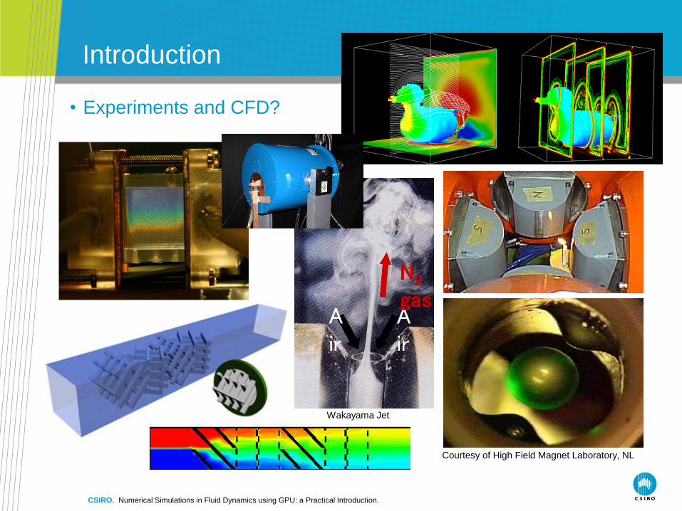
Introduction
• Experiments and CFD?
CSIRO. Numerical Simulations in Fluid Dynamics using GPU: a Practical Introduction.
Courtesy of High Field Magnet Laboratory, NL
Air
Air
N2
gas
Wakayama Jet

Exchange Flows in Reservoirs – Cooling Case
• Water circulation in reservoirs is driven by thermal gradients changing
during day and night cycles.

0
1
2
3
4
5
0 10 20 30 40 50
t [s]
dT
[m
m]
dT ~ (k t )0.5 at Gr = 7.82x10³ and Pr = 6.91
dT ~ (k t )0.5 at Gr = 2.04x10⁴ and Pr = 8.05
CSIRO. Insert presentation title, do not remove CSIRO from start of footer
dT ~ (k · t)1/2 Scaling relation:
Exchange Flows in Reservoirs – Cooling Case
t = 100[s]
t = 200[s]
t = 500[s]
t = 700[s]
t = 1000[s]
t = 4000[s]

17
18
19
20
21
22
23
24
0 7 14 21 28 35 42 49 56 63 70
Time [min]
Tem
pera
ture
[oC
] a
b
c
d
e
f
g
h
i
j
k
Exchange Flows in Reservoirs – Diurnal Case
Pr = 6.82,
Gr = 3.52×10⁴
9
Dt
PIV result
unsharp mask
CSIRO. Numerical Simulations in Fluid Dynamics using GPU: a Practical Introduction.

DEM and SPH examples
CSIRO. Numerical Simulations in Fluid Dynamics using GPU: a Practical Introduction.
Courtesy of Paul Cleary Computational Modelling
Group

CSIRO. Numerical Simulations in Fluid Dynamics using GPU: a Practical Introduction.
Equations Discretisation
Implementation Verification
Results Transfer CPU code to
GPU code Verification Results!
Process
Governing Equations,
Discretisation Procedure,
Algorithms.
CSIRO. Numerical Simulations in Fluid Dynamics using GPU: a Practical Introduction.

Governing equations (dimensional)
• Continuity equation
𝜕𝑢
𝜕𝑥+𝜕𝑣
𝜕𝑦= 0
𝜕𝑢
𝜕𝑡+ 𝑢
𝜕𝑢
𝜕𝑥+ 𝑣
𝜕𝑢
𝜕𝑦= −
1
𝜌
𝜕𝑝
𝜕𝑥+ ν
𝜕2𝑢
𝜕𝑥2 +𝜕2𝑢
𝜕𝑦2 + 𝑏𝑜𝑑𝑦_𝑓𝑜𝑟𝑐𝑒_𝑥
• Momentum equations
𝜕𝑣
𝜕𝑡+ 𝑢
𝜕𝑣
𝜕𝑥+ 𝑣
𝜕𝑣
𝜕𝑦= −
1
𝜌
𝜕𝑝
𝜕𝑦+ ν
𝜕2𝑣
𝜕𝑥2 +𝜕2𝑣
𝜕𝑦2 + 𝑏𝑜𝑑𝑦_𝑓𝑜𝑟𝑐𝑒_𝑦
• Energy equation
𝜕𝑇
𝜕𝑡+ 𝑢
𝜕𝑇
𝜕𝑥+ 𝑣
𝜕𝑇
𝜕𝑦= 𝛼
𝜕2𝑇
𝜕𝑥2 +𝜕2𝑇
𝜕𝑦2
CSIRO. Numerical Simulations in Fluid Dynamics using GPU: a Practical Introduction.
unsteady
acceleration
convective
acceleration pressure
gradient
viscous
term body
force
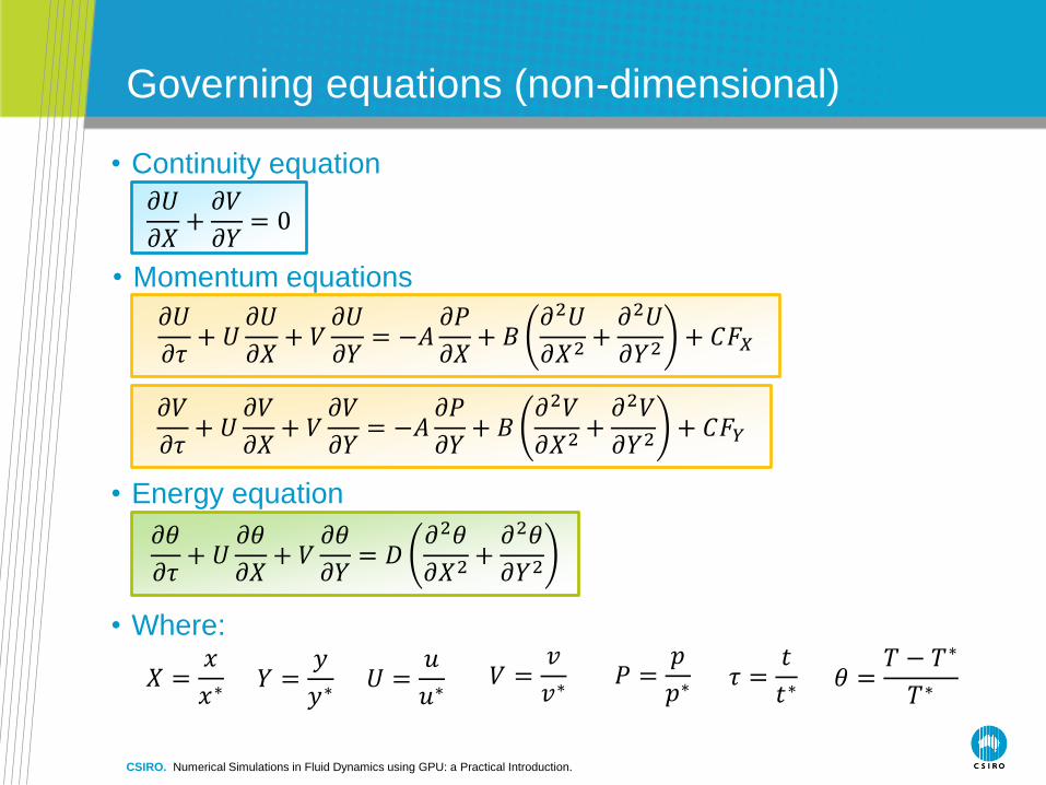
• Continuity equation
𝜕𝑈
𝜕𝑋+𝜕𝑉
𝜕𝑌= 0
Governing equations (non-dimensional)
• Momentum equations
CSIRO. Numerical Simulations in Fluid Dynamics using GPU: a Practical Introduction.
𝜕𝑈
𝜕𝜏+ 𝑈
𝜕𝑈
𝜕𝑋+ 𝑉
𝜕𝑈
𝜕𝑌= −𝐴
𝜕𝑃
𝜕𝑋+ 𝐵
𝜕2𝑈
𝜕𝑋2 +𝜕2𝑈
𝜕𝑌2 + 𝐶𝐹𝑋
𝜕𝑉
𝜕𝜏+ 𝑈
𝜕𝑉
𝜕𝑋+ 𝑉
𝜕𝑉
𝜕𝑌= −𝐴
𝜕𝑃
𝜕𝑌+ 𝐵
𝜕2𝑉
𝜕𝑋2 +𝜕2𝑉
𝜕𝑌2 + 𝐶𝐹𝑌
𝜕𝜃
𝜕𝜏+ 𝑈
𝜕𝜃
𝜕𝑋+ 𝑉
𝜕𝜃
𝜕𝑌= 𝐷
𝜕2𝜃
𝜕𝑋2 +𝜕2𝜃
𝜕𝑌2
• Energy equation
𝑈 =𝑢
𝑢∗
• Where:
𝑉 =𝑣
𝑣∗ 𝑋 =
𝑥
𝑥∗ 𝑌 =𝑦
𝑦∗ 𝑃 =
𝑝
𝑝∗ 𝜏 =
𝑡
𝑡∗ 𝜃 =
𝑇 − 𝑇∗
𝑇∗

Staggered grid
𝑝𝑖,𝑗 𝑝𝑖+1,𝑗
𝑝𝑖,𝑗+1 𝑝𝑖+1,𝑗+1
𝑣𝑖,𝑗 𝑣𝑖+1,𝑗
𝑣𝑖+1,𝑗+1 𝑣𝑖,𝑗+1
𝑢𝑖,𝑗
𝑢𝑖,𝑗+1
𝑢𝑖+1,𝑗+1
𝑢𝑖+1,𝑗
𝒊 𝒊 + 𝟏
𝒋
𝒋 + 𝟏
𝒄𝒆𝒍𝒍(𝒊, 𝒋)
• Different variables are located at
different locations:
• scalar variables (pressure,
temperature, concentration) are
stored at the centre of the cell,
• the horizontal velocity component is
sampled at the centre of the vertical
cell face,
• the vertical velocity component is
sampled at the centre of the
horizontal cell face.
• The discrete values of u, v and p can be thought as located on three
separate grids, each shifted by half grid spacing to the bottom, to the
left, and to the lower left respectively.
• The staggered arrangement of the unknowns prevents possible
pressure oscillations.
CSIRO. Numerical Simulations in Fluid Dynamics using GPU: a Practical Introduction.
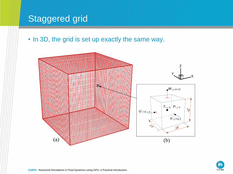
Staggered grid
• In 3D, the grid is set up exactly the same way.
CSIRO. Numerical Simulations in Fluid Dynamics using GPU: a Practical Introduction.
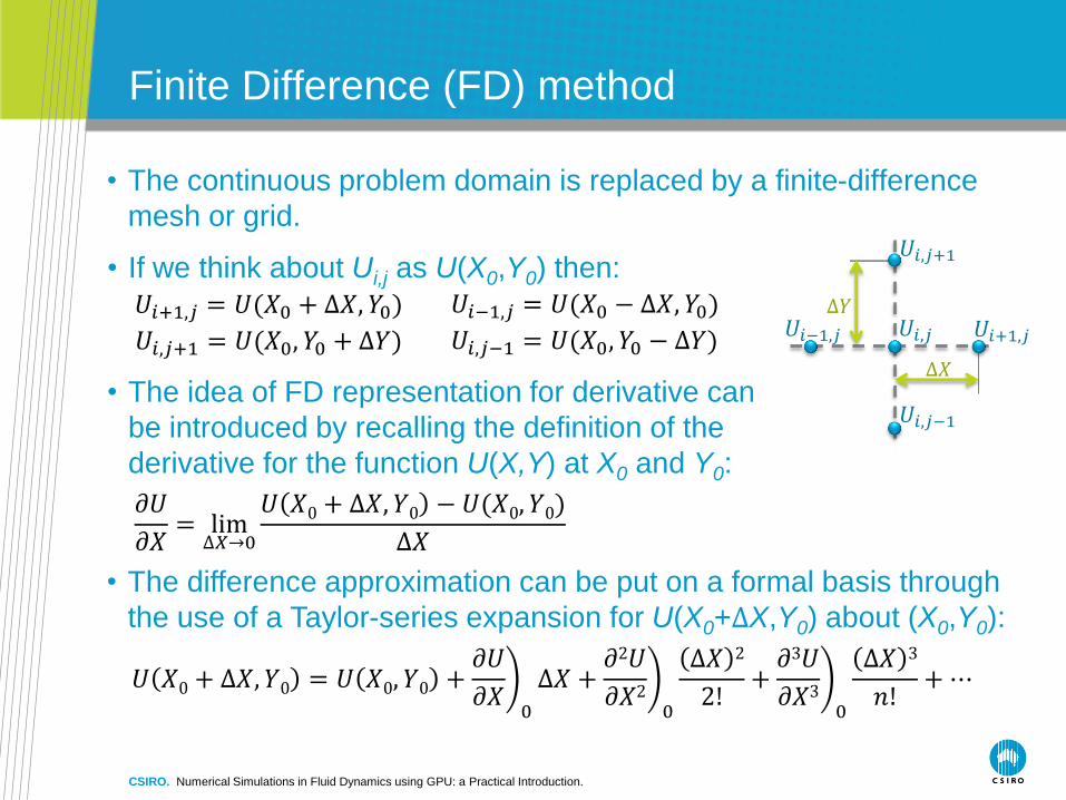
Finite Difference (FD) method
• The continuous problem domain is replaced by a finite-difference
mesh or grid.
𝑈𝑖,𝑗 𝑈𝑖+1,𝑗 𝑈𝑖−1,𝑗
𝑈𝑖,𝑗+1
𝑈𝑖,𝑗−1
∆𝑋
∆𝑌
• If we think about Ui,j as U(X0,Y0) then:
𝑈𝑖+1,𝑗 = 𝑈(𝑋0 + ∆𝑋, 𝑌0)
𝑈𝑖,𝑗+1 = 𝑈(𝑋0, 𝑌0 + ∆𝑌)
𝑈𝑖−1,𝑗 = 𝑈(𝑋0 − ∆𝑋, 𝑌0)
𝑈𝑖,𝑗−1 = 𝑈(𝑋0, 𝑌0 − ∆𝑌)
• The idea of FD representation for derivative can
be introduced by recalling the definition of the
derivative for the function U(X,Y) at X0 and Y0:
𝜕𝑈
𝜕𝑋= lim
∆𝑋→0
𝑈 𝑋0 + ∆𝑋, 𝑌0 − 𝑈(𝑋0, 𝑌0)
∆𝑋
• The difference approximation can be put on a formal basis through
the use of a Taylor-series expansion for U(X0+∆X,Y0) about (X0,Y0):
𝑈 𝑋0 + ∆𝑋, 𝑌0 = 𝑈 𝑋0, 𝑌0 +𝜕𝑈
𝜕𝑋 0
∆𝑋 +𝜕2𝑈
𝜕𝑋2 0
∆𝑋 2
2!+𝜕3𝑈
𝜕𝑋3 0
∆𝑋 3
𝑛!+ ⋯
CSIRO. Numerical Simulations in Fluid Dynamics using GPU: a Practical Introduction.

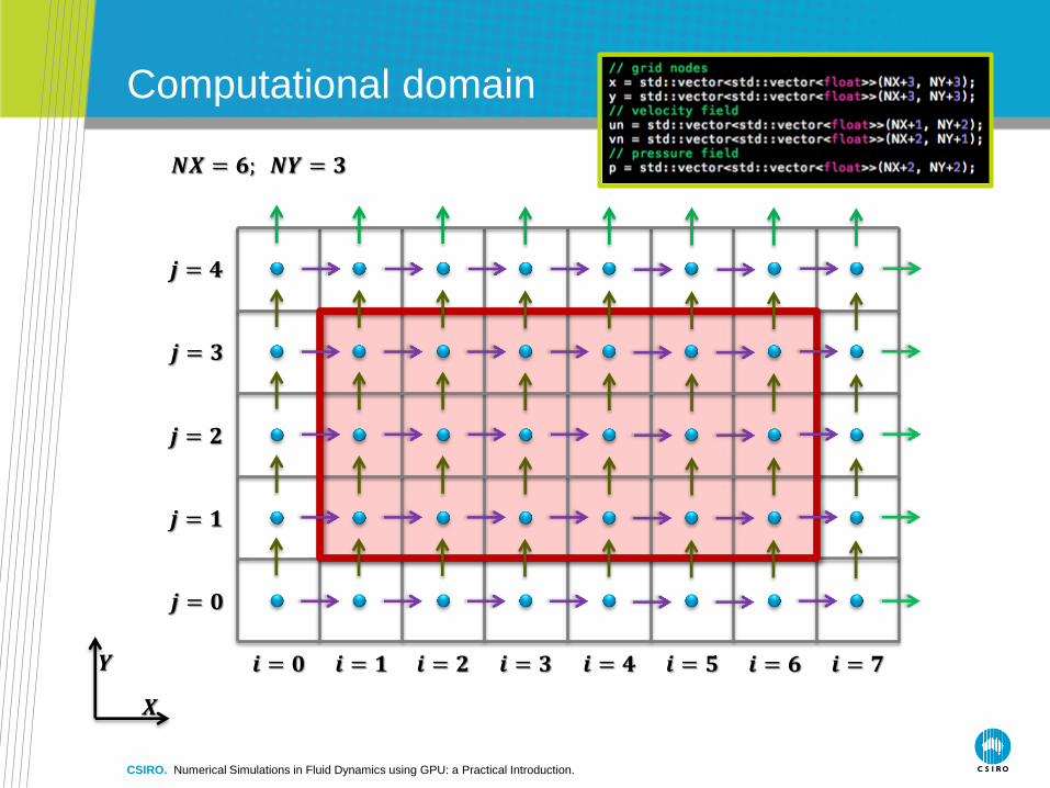
Computational domain
𝒊 = 𝟎 𝒊 = 𝟏 𝒊 = 𝟐 𝒊 = 𝟑 𝒊 = 𝟒 𝒊 = 𝟓 𝒊 = 𝟔 𝒊 = 𝟕
𝒋 = 𝟒
𝒋 = 𝟑
𝒋 = 𝟐
𝒋 = 𝟏
𝒋 = 𝟎
𝑵𝑿 = 𝟔; 𝑵𝒀 = 𝟑
CSIRO. Numerical Simulations in Fluid Dynamics using GPU: a Practical Introduction.
boundary strip
boundary of computational domain
computational domain
𝑿
𝒀
Computational domain
𝒊 = 𝟎 𝒊 = 𝟏 𝒊 = 𝟐 𝒊 = 𝟑 𝒊 = 𝟒 𝒊 = 𝟓 𝒊 = 𝟔 𝒊 = 𝟕
𝒋 = 𝟒
𝒋 = 𝟑
𝒋 = 𝟐
𝒋 = 𝟏
𝒋 = 𝟎
CSIRO. Numerical Simulations in Fluid Dynamics using GPU: a Practical Introduction.
𝑵𝑿 = 𝟔; 𝑵𝒀 = 𝟑
𝑿
𝒀

Discretisation of the continuity equation
• Continuity equation:
CSIRO. Numerical Simulations in Fluid Dynamics using GPU: a Practical Introduction.
𝜕𝑈
𝜕𝑋+𝜕𝑉
𝜕𝑌= 0
𝜕𝑈
𝜕𝑋=
𝑈𝑒 − 𝑈𝑤
∆𝑋
𝜕𝑉
𝜕𝑌=
𝑉𝑛 − 𝑉𝑠∆𝑌
𝜕𝑈
𝜕𝑋+𝜕𝑉
𝜕𝑌=
𝑈𝑖,𝑗 − 𝑈𝑖−1,𝑗
∆𝑋+𝑉𝑖,𝑗 − 𝑉𝑖,𝑗−1
∆𝑌= 0
• All derivatives are calculated at the centre of the cell.
∆𝑌
𝑉𝑛
𝑉𝑠
∆𝑋
𝑈𝑒 𝑈𝑤 𝑈𝑒 = 𝑈𝑖,𝑗
𝑈𝑤 = 𝑈𝑖−1,𝑗
𝑉𝑛 = 𝑉𝑖,𝑗 𝑉𝑠 = 𝑉𝑖,𝑗−1

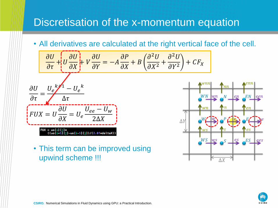
Discretisation of the x-momentum equation
CSIRO. Numerical Simulations in Fluid Dynamics using GPU: a Practical Introduction.
• All derivatives are calculated at the right vertical face of the cell.
𝜕𝑈
𝜕𝜏+ 𝑈
𝜕𝑈
𝜕𝑋+ 𝑉
𝜕𝑈
𝜕𝑌= −𝐴
𝜕𝑃
𝜕𝑋+ 𝐵
𝜕2𝑈
𝜕𝑋2 +𝜕2𝑈
𝜕𝑌2 + 𝐶𝐹𝑋
𝑃 𝐸 𝑊
𝑁
𝑆
𝐸𝑁
𝐸𝑆
𝑊𝑁
𝑊𝑆
𝑒 𝑤 𝑒𝑒
𝑒𝑛
𝑒𝑠
𝑤𝑛
𝑤𝑠
𝑛
𝑠
𝑛𝑛
𝑤𝑛
𝑤𝑠
𝑒𝑛
𝑒𝑠
𝑤𝑛𝑛 𝑒𝑛𝑛
𝑒𝑒𝑛
𝑒𝑒𝑠
𝜕𝑈
𝜕𝜏=
𝑈𝑒𝑘+1 − 𝑈𝑒
𝑘
∆𝜏
∆𝑌
∆𝑋
• Time advancement.
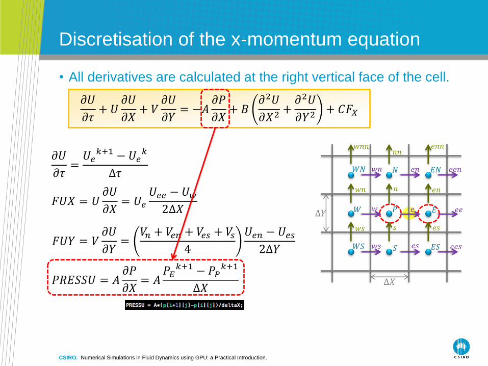
Discretisation of the x-momentum equation
CSIRO. Numerical Simulations in Fluid Dynamics using GPU: a Practical Introduction.
• All derivatives are calculated at the right vertical face of the cell.
𝜕𝑈
𝜕𝜏+ 𝑈
𝜕𝑈
𝜕𝑋+ 𝑉
𝜕𝑈
𝜕𝑌= −𝐴
𝜕𝑃
𝜕𝑋+ 𝐵
𝜕2𝑈
𝜕𝑋2 +𝜕2𝑈
𝜕𝑌2 + 𝐶𝐹𝑋
𝑃 𝐸 𝑊
𝑁
𝑆
𝐸𝑁
𝐸𝑆
𝑊𝑁
𝑊𝑆
𝑒 𝑤 𝑒𝑒
𝑒𝑛
𝑒𝑠
𝑤𝑛
𝑤𝑠
𝑛
𝑠
𝑛𝑛
𝑤𝑛
𝑤𝑠
𝑒𝑛
𝑒𝑠
𝑤𝑛𝑛 𝑒𝑛𝑛
𝑒𝑒𝑛
𝑒𝑒𝑠
𝜕𝑈
𝜕𝜏=
𝑈𝑒𝑘+1 − 𝑈𝑒
𝑘
∆𝜏
𝐹𝑈𝑋 = 𝑈𝜕𝑈
𝜕𝑋= 𝑈𝑒
𝑈𝑒𝑒 − 𝑈𝑤
2∆𝑋
∆𝑌
∆𝑋
• This term can be improved using
upwind scheme !!!

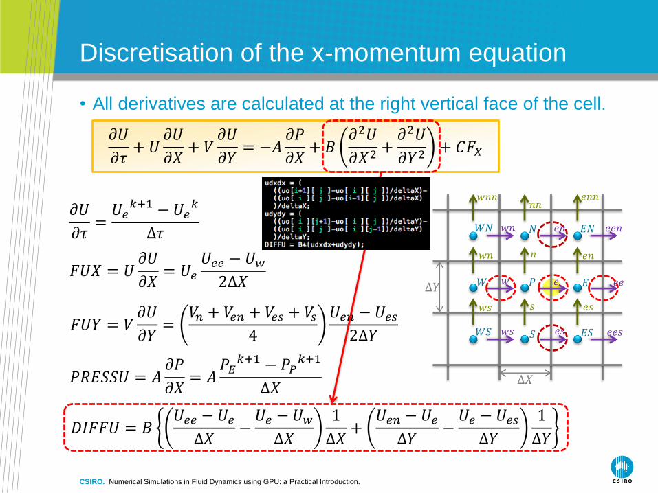
Discretisation of the x-momentum equation
CSIRO. Numerical Simulations in Fluid Dynamics using GPU: a Practical Introduction.
• All derivatives are calculated at the right vertical face of the cell.
𝜕𝑈
𝜕𝜏+ 𝑈
𝜕𝑈
𝜕𝑋+ 𝑉
𝜕𝑈
𝜕𝑌= −𝐴
𝜕𝑃
𝜕𝑋+ 𝐵
𝜕2𝑈
𝜕𝑋2 +𝜕2𝑈
𝜕𝑌2 + 𝐶𝐹𝑋
𝑃 𝐸 𝑊
𝑁
𝑆
𝐸𝑁
𝐸𝑆
𝑊𝑁
𝑊𝑆
𝑒 𝑤 𝑒𝑒
𝑒𝑛
𝑒𝑠
𝑤𝑛
𝑤𝑠
𝑛
𝑠
𝑛𝑛
𝑤𝑛
𝑤𝑠
𝑒𝑛
𝑒𝑠
𝑤𝑛𝑛 𝑒𝑛𝑛
𝑒𝑒𝑛
𝑒𝑒𝑠
𝜕𝑈
𝜕𝜏=
𝑈𝑒𝑘+1 − 𝑈𝑒
𝑘
∆𝜏
𝐹𝑈𝑋 = 𝑈𝜕𝑈
𝜕𝑋= 𝑈𝑒
𝑈𝑒𝑒 − 𝑈𝑤
2∆𝑋
𝐹𝑈𝑌 = 𝑉𝜕𝑈
𝜕𝑌=
𝑉𝑛 + 𝑉𝑒𝑛 + 𝑉𝑒𝑠 + 𝑉𝑠4
𝑈𝑒𝑛 − 𝑈𝑒𝑠
2∆𝑌
∆𝑌
∆𝑋
• This term can be improved using
upwind scheme !!!
Discretisation of the x-momentum equation
CSIRO. Numerical Simulations in Fluid Dynamics using GPU: a Practical Introduction.
• All derivatives are calculated at the right vertical face of the cell.
𝜕𝑈
𝜕𝜏+ 𝑈
𝜕𝑈
𝜕𝑋+ 𝑉
𝜕𝑈
𝜕𝑌= −𝐴
𝜕𝑃
𝜕𝑋+ 𝐵
𝜕2𝑈
𝜕𝑋2 +𝜕2𝑈
𝜕𝑌2 + 𝐶𝐹𝑋
𝑃 𝐸 𝑊
𝑁
𝑆
𝐸𝑁
𝐸𝑆
𝑊𝑁
𝑊𝑆
𝑒 𝑤 𝑒𝑒
𝑒𝑛
𝑒𝑠
𝑤𝑛
𝑤𝑠
𝑛
𝑠
𝑛𝑛
𝑤𝑛
𝑤𝑠
𝑒𝑛
𝑒𝑠
𝑤𝑛𝑛 𝑒𝑛𝑛
𝑒𝑒𝑛
𝑒𝑒𝑠
𝜕𝑈
𝜕𝜏=
𝑈𝑒𝑘+1 − 𝑈𝑒
𝑘
∆𝜏
𝐹𝑈𝑋 = 𝑈𝜕𝑈
𝜕𝑋= 𝑈𝑒
𝑈𝑒𝑒 − 𝑈𝑤
2∆𝑋
𝐹𝑈𝑌 = 𝑉𝜕𝑈
𝜕𝑌=
𝑉𝑛 + 𝑉𝑒𝑛 + 𝑉𝑒𝑠 + 𝑉𝑠4
𝑈𝑒𝑛 − 𝑈𝑒𝑠
2∆𝑌
𝑃𝑅𝐸𝑆𝑆𝑈 = 𝐴𝜕𝑃
𝜕𝑋= 𝐴
𝑃𝐸𝑘+1 − 𝑃𝑃
𝑘+1
∆𝑋
∆𝑌
∆𝑋
Discretisation of the x-momentum equation
CSIRO. Numerical Simulations in Fluid Dynamics using GPU: a Practical Introduction.
• All derivatives are calculated at the right vertical face of the cell.
𝜕𝑈
𝜕𝜏+ 𝑈
𝜕𝑈
𝜕𝑋+ 𝑉
𝜕𝑈
𝜕𝑌= −𝐴
𝜕𝑃
𝜕𝑋+ 𝐵
𝜕2𝑈
𝜕𝑋2 +𝜕2𝑈
𝜕𝑌2 + 𝐶𝐹𝑋
𝑃 𝐸 𝑊
𝑁
𝑆
𝐸𝑁
𝐸𝑆
𝑊𝑁
𝑊𝑆
𝑒 𝑤 𝑒𝑒
𝑒𝑛
𝑒𝑠
𝑤𝑛
𝑤𝑠
𝑛
𝑠
𝑛𝑛
𝑤𝑛
𝑤𝑠
𝑒𝑛
𝑒𝑠
𝑤𝑛𝑛 𝑒𝑛𝑛
𝑒𝑒𝑛
𝑒𝑒𝑠
𝜕𝑈
𝜕𝜏=
𝑈𝑒𝑘+1 − 𝑈𝑒
𝑘
∆𝜏
𝐹𝑈𝑋 = 𝑈𝜕𝑈
𝜕𝑋= 𝑈𝑒
𝑈𝑒𝑒 − 𝑈𝑤
2∆𝑋
𝐹𝑈𝑌 = 𝑉𝜕𝑈
𝜕𝑌=
𝑉𝑛 + 𝑉𝑒𝑛 + 𝑉𝑒𝑠 + 𝑉𝑠4
𝑈𝑒𝑛 − 𝑈𝑒𝑠
2∆𝑌
𝑃𝑅𝐸𝑆𝑆𝑈 = 𝐴𝜕𝑃
𝜕𝑋= 𝐴
𝑃𝐸𝑘+1 − 𝑃𝑃
𝑘+1
∆𝑋
𝐷𝐼𝐹𝐹𝑈 = 𝐵𝑈𝑒𝑒 − 𝑈𝑒
∆𝑋−𝑈𝑒 − 𝑈𝑤
∆𝑋
1
∆𝑋+
𝑈𝑒𝑛 − 𝑈𝑒
∆𝑌−𝑈𝑒 − 𝑈𝑒𝑠
∆𝑌
1
∆𝑌
∆𝑌
∆𝑋
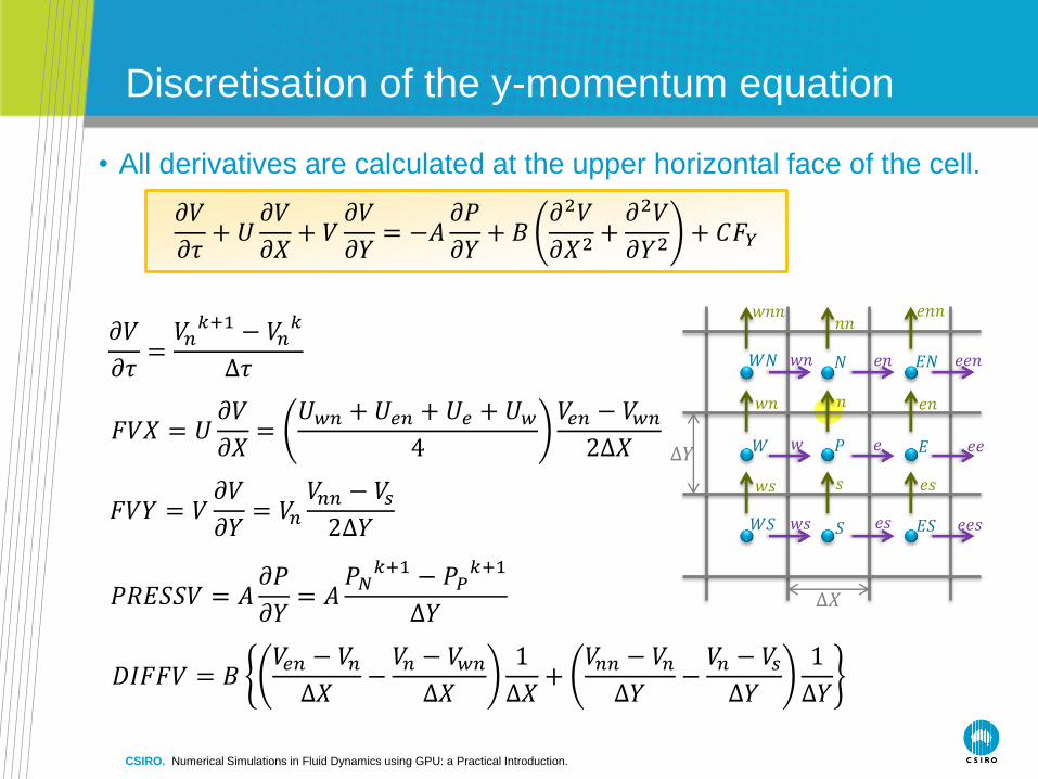
𝜕𝑉
𝜕𝜏+ 𝑈
𝜕𝑉
𝜕𝑋+ 𝑉
𝜕𝑉
𝜕𝑌= −𝐴
𝜕𝑃
𝜕𝑌+ 𝐵
𝜕2𝑉
𝜕𝑋2 +𝜕2𝑉
𝜕𝑌2 + 𝐶𝐹𝑌
Discretisation of the y-momentum equation
CSIRO. Numerical Simulations in Fluid Dynamics using GPU: a Practical Introduction.
𝑃 𝐸 𝑊
𝑁
𝑆
𝐸𝑁
𝐸𝑆
𝑊𝑁
𝑊𝑆
𝑒 𝑤 𝑒𝑒
𝑒𝑛
𝑒𝑠
𝑤𝑛
𝑤𝑠
𝑛
𝑠
𝑛𝑛
𝑤𝑛
𝑤𝑠
𝑒𝑛
𝑒𝑠
𝑤𝑛𝑛 𝑒𝑛𝑛
𝑒𝑒𝑛
𝑒𝑒𝑠
𝐷𝐼𝐹𝐹𝑉 = 𝐵𝑉𝑒𝑛 − 𝑉𝑛
∆𝑋−𝑉𝑛 − 𝑉𝑤𝑛
∆𝑋
1
∆𝑋+
𝑉𝑛𝑛 − 𝑉𝑛∆𝑌
−𝑉𝑛 − 𝑉𝑠∆𝑌
1
∆𝑌
∆𝑌
∆𝑋 𝑃𝑅𝐸𝑆𝑆𝑉 = 𝐴𝜕𝑃
𝜕𝑌= 𝐴
𝑃𝑁𝑘+1 − 𝑃𝑃
𝑘+1
∆𝑌
𝐹𝑉𝑌 = 𝑉𝜕𝑉
𝜕𝑌= 𝑉𝑛
𝑉𝑛𝑛 − 𝑉𝑠2∆𝑌
𝐹𝑉𝑋 = 𝑈𝜕𝑉
𝜕𝑋=
𝑈𝑤𝑛 + 𝑈𝑒𝑛 + 𝑈𝑒 + 𝑈𝑤
4
𝑉𝑒𝑛 − 𝑉𝑤𝑛
2∆𝑋
𝜕𝑉
𝜕𝜏=
𝑉𝑛𝑘+1 − 𝑉𝑛
𝑘
∆𝜏
• All derivatives are calculated at the upper horizontal face of the cell.
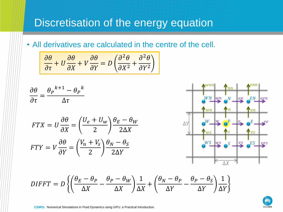
𝜕𝜃
𝜕𝜏+ 𝑈
𝜕𝜃
𝜕𝑋+ 𝑉
𝜕𝜃
𝜕𝑌= 𝐷
𝜕2𝜃
𝜕𝑋2 +𝜕2𝜃
𝜕𝑌2
Discretisation of the energy equation
CSIRO. Numerical Simulations in Fluid Dynamics using GPU: a Practical Introduction.
𝑃 𝐸 𝑊
𝑁
𝑆
𝐸𝑁
𝐸𝑆
𝑊𝑁
𝑊𝑆
𝑒 𝑤 𝑒𝑒
𝑒𝑛
𝑒𝑠
𝑤𝑛
𝑤𝑠
𝑛
𝑠
𝑛𝑛
𝑤𝑛
𝑤𝑠
𝑒𝑛
𝑒𝑠
𝑤𝑛𝑛 𝑒𝑛𝑛
𝑒𝑒𝑛
𝑒𝑒𝑠
𝐷𝐼𝐹𝐹𝑇 = 𝐷𝜃𝐸 − 𝜃𝑃
∆𝑋−𝜃𝑃 − 𝜃𝑊
∆𝑋
1
∆𝑋+
𝜃𝑁 − 𝜃𝑃∆𝑌
−𝜃𝑃 − 𝜃𝑆∆𝑌
1
∆𝑌
∆𝑌
∆𝑋
𝜕𝜃
𝜕𝜏=
𝜃𝑃𝑘+1 − 𝜃𝑃
𝑘
∆𝜏
• All derivatives are calculated in the centre of the cell.
𝐹𝑇𝑋 = 𝑈𝜕𝜃
𝜕𝑋=
𝑈𝑒 + 𝑈𝑤
2
𝜃𝐸 − 𝜃𝑊2∆𝑋
𝐹𝑇𝑌 = 𝑉𝜕𝜃
𝜕𝑌=
𝑉𝑛 + 𝑉𝑠2
𝜃𝑁 − 𝜃𝑆2∆𝑌
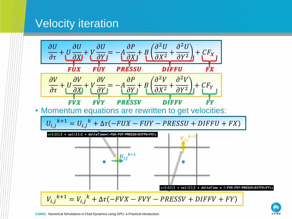
Velocity iteration
𝜕𝑈
𝜕𝜏+ 𝑈
𝜕𝑈
𝜕𝑋+ 𝑉
𝜕𝑈
𝜕𝑌= −𝐴
𝜕𝑃
𝜕𝑋+ 𝐵
𝜕2𝑈
𝜕𝑋2 +𝜕2𝑈
𝜕𝑌2 + 𝐶𝐹𝑋
𝜕𝑉
𝜕𝜏+ 𝑈
𝜕𝑉
𝜕𝑋+ 𝑉
𝜕𝑉
𝜕𝑌= −𝐴
𝜕𝑃
𝜕𝑌+ 𝐵
𝜕2𝑉
𝜕𝑋2 +𝜕2𝑉
𝜕𝑌2 + 𝐶𝐹𝑌
𝑭𝑼𝑿 𝑭𝑼𝒀 𝑷𝑹𝑬𝑺𝑺𝑼 𝑫𝑰𝑭𝑭𝑼 𝑭𝑿
𝑭𝑽𝑿 𝑭𝑽𝒀 𝑷𝑹𝑬𝑺𝑺𝑽 𝑫𝑰𝑭𝑭𝑽 𝑭𝒀
• Momentum equations are rewritten to get velocities:
𝑈𝑖,𝑗𝑘+1 = 𝑈𝑖,𝑗
𝑘 + ∆𝜏 −𝐹𝑈𝑋 − 𝐹𝑈𝑌 − 𝑃𝑅𝐸𝑆𝑆𝑈 + 𝐷𝐼𝐹𝐹𝑈 + 𝐹𝑋
𝑉𝑖,𝑗𝑘+1 = 𝑉𝑖,𝑗
𝑘 + ∆𝜏 −𝐹𝑉𝑋 − 𝐹𝑉𝑌 − 𝑃𝑅𝐸𝑆𝑆𝑉 + 𝐷𝐼𝐹𝐹𝑉 + 𝐹𝑌
𝑼𝒊,𝒋𝒌+𝟏
𝑽𝒊,𝒋𝒌+𝟏
CSIRO. Numerical Simulations in Fluid Dynamics using GPU: a Practical Introduction.
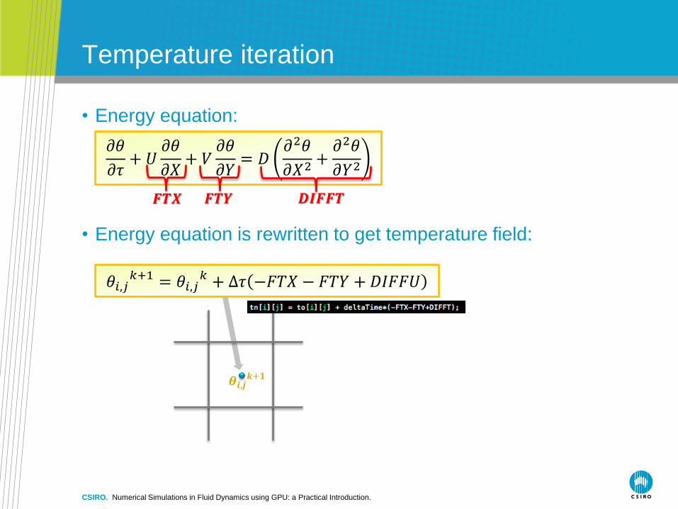
𝜕𝜃
𝜕𝜏+ 𝑈
𝜕𝜃
𝜕𝑋+ 𝑉
𝜕𝜃
𝜕𝑌= 𝐷
𝜕2𝜃
𝜕𝑋2 +𝜕2𝜃
𝜕𝑌2
Temperature iteration
𝑭𝑻𝑿 𝑭𝑻𝒀 𝑫𝑰𝑭𝑭𝑻
• Energy equation is rewritten to get temperature field:
𝜃𝑖,𝑗𝑘+1 = 𝜃𝑖,𝑗
𝑘 + ∆𝜏 −𝐹𝑇𝑋 − 𝐹𝑇𝑌 + 𝐷𝐼𝐹𝐹𝑈
𝜽𝒊,𝒋𝒌+𝟏
• Energy equation:
CSIRO. Numerical Simulations in Fluid Dynamics using GPU: a Practical Introduction.

OUTER LOOP
Flow Chart of the CPU Fluid Solver
START
Read Configuration
Allocate Memory for Flow
Field Tables
Apply Boundary
Conditions (BC)
Calculate Tentative
Velocities (U, V)
Calculate Pressure
Correction
Correct Pressure and
Velocity Fields, Apply BC
Converged? NO
Calculate Energy
Equation (if required)
YES
Final time
achieved?
Advance All Flow Tables
and Increase Time
NO
Save Results: Flow
Fields, etc...
FINISH
YES
INNER LOOP
CSIRO. Numerical Simulations in Fluid Dynamics using GPU: a Practical Introduction.
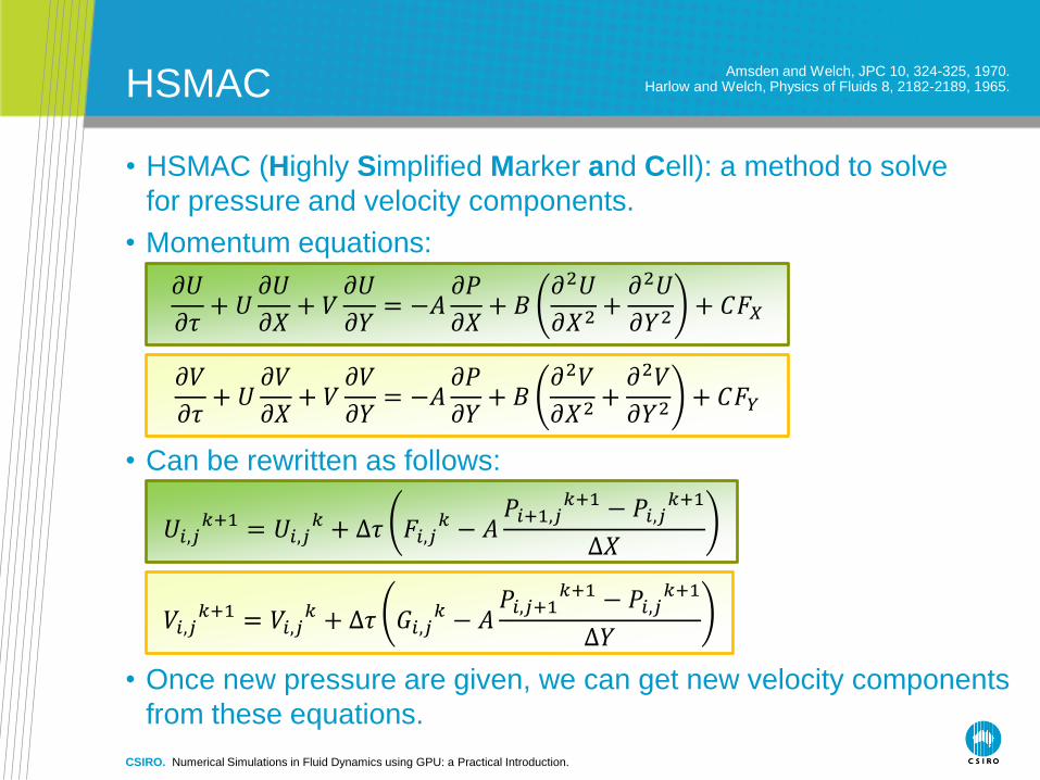
HSMAC
• HSMAC (Highly Simplified Marker and Cell): a method to solve
for pressure and velocity components.
CSIRO. Numerical Simulations in Fluid Dynamics using GPU: a Practical Introduction.
𝜕𝑈
𝜕𝜏+ 𝑈
𝜕𝑈
𝜕𝑋+ 𝑉
𝜕𝑈
𝜕𝑌= −𝐴
𝜕𝑃
𝜕𝑋+ 𝐵
𝜕2𝑈
𝜕𝑋2 +𝜕2𝑈
𝜕𝑌2 + 𝐶𝐹𝑋
𝜕𝑉
𝜕𝜏+ 𝑈
𝜕𝑉
𝜕𝑋+ 𝑉
𝜕𝑉
𝜕𝑌= −𝐴
𝜕𝑃
𝜕𝑌+ 𝐵
𝜕2𝑉
𝜕𝑋2 +𝜕2𝑉
𝜕𝑌2 + 𝐶𝐹𝑌
• Momentum equations:
• Can be rewritten as follows:
𝑈𝑖,𝑗𝑘+1 = 𝑈𝑖,𝑗
𝑘 + ∆𝜏 𝐹𝑖,𝑗𝑘 − 𝐴
𝑃𝑖+1,𝑗𝑘+1 − 𝑃𝑖,𝑗
𝑘+1
∆𝑋
𝑉𝑖,𝑗𝑘+1 = 𝑉𝑖,𝑗
𝑘 + ∆𝜏 𝐺𝑖,𝑗𝑘 − 𝐴
𝑃𝑖,𝑗+1𝑘+1 − 𝑃𝑖,𝑗
𝑘+1
∆𝑌
• Once new pressure are given, we can get new velocity components
from these equations.
Harlow and Welch, Physics of Fluids 8, 2182-2189, 1965. Amsden and Welch, JPC 10, 324-325, 1970.
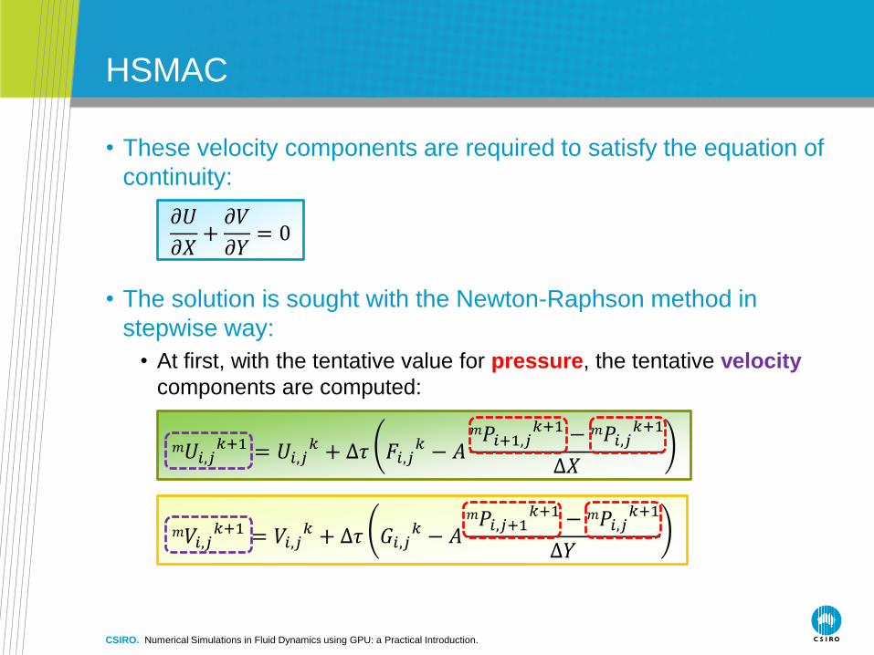
HSMAC
• These velocity components are required to satisfy the equation of
continuity:
𝜕𝑈
𝜕𝑋+𝜕𝑉
𝜕𝑌= 0
• The solution is sought with the Newton-Raphson method in
stepwise way:
• At first, with the tentative value for pressure, the tentative velocity
components are computed:
𝑚𝑈𝑖,𝑗𝑘+1 = 𝑈𝑖,𝑗
𝑘 + ∆𝜏 𝐹𝑖,𝑗𝑘 − 𝐴
𝑚𝑃𝑖+1,𝑗𝑘+1 − 𝑚𝑃𝑖,𝑗
𝑘+1
∆𝑋
𝑚𝑉𝑖,𝑗𝑘+1 = 𝑉𝑖,𝑗
𝑘 + ∆𝜏 𝐺𝑖,𝑗𝑘 − 𝐴
𝑚𝑃𝑖,𝑗+1𝑘+1 − 𝑚𝑃𝑖,𝑗
𝑘+1
∆𝑌
CSIRO. Numerical Simulations in Fluid Dynamics using GPU: a Practical Introduction.

HSMAC
• The tentative velocity and the pressure fields need to be corrected to
give better approximation at step m+1:
CSIRO. Numerical Simulations in Fluid Dynamics using GPU: a Practical Introduction.
𝑈𝑚+1 𝑘+1 = 𝑈𝑚 𝑘+1 + 𝑈′
𝑉𝑚+1 𝑘+1 = 𝑉𝑚 𝑘+1 + 𝑉′
𝑃𝑚+1 𝑘+1 = 𝑃𝑚 𝑘+1 + 𝑃′
• Then, the LHS of continuity equation is expressed as:
𝐷𝑚+1𝑖,𝑗𝑘+1 =
𝑈𝑚+1𝑖,𝑗𝑘+1 − 𝑈𝑚+1
𝑖−1,𝑗𝑘+1
∆𝑋+
𝑉𝑚+1𝑖,𝑗𝑘+1 − 𝑉𝑚+1
𝑖,𝑗−1𝑘+1
∆𝑌
𝐷𝑚𝑖,𝑗𝑘+1 =
𝑈𝑚𝑖,𝑗𝑘+1 − 𝑈𝑚
𝑖−1,𝑗𝑘+1
∆𝑋+
𝑉𝑚𝑖,𝑗𝑘+1 − 𝑉𝑚
𝑖,𝑗−1𝑘+1
∆𝑌
• The equation of continuity is to be satisfied in the new time step (𝑘 + 1)∆𝜏
so let us assume 𝐷𝑖,𝑗𝑘+1 = 0 though 𝐷𝑖,𝑗
𝑘 ≠ 0 with the non-convergent
incorrect velocity components for 𝑈 and 𝑉.
• Newton-Raphson method provides the stepwise approach for the
solution to satisfy 𝐷𝑖,𝑗𝑘+1 = 0.

HSMAC
• These are inserted in continuity equation:
𝑚𝑈𝑖,𝑗𝑘+1 = 𝑈𝑖,𝑗
𝑘 + ∆𝜏 𝐹𝑖,𝑗𝑘 −
𝑚𝑃𝑖+1,𝑗𝑘+1 − 𝑚𝑃𝑖,𝑗
𝑘+1
∆𝑋
𝑚𝑉𝑖,𝑗𝑘+1 = 𝑉𝑖,𝑗
𝑘 + ∆𝜏 𝐺𝑖,𝑗𝑘 −
𝑚𝑃𝑖,𝑗+1𝑘+1 − 𝑚𝑃𝑖,𝑗
𝑘+1
∆𝑌
𝑈𝑖,𝑗𝑘+1 − 𝑈𝑖−1,𝑗
𝑘+1
∆𝑋+𝑉𝑖,𝑗𝑘+1 − 𝑉𝑖,𝑗−1
𝑘+1
∆𝑌=
𝑈𝑖,𝑗𝑘 − 𝑈𝑖−1,𝑗
𝑘
∆𝑋+𝑉𝑖,𝑗𝑘 − 𝑉𝑖,𝑗−1
𝑘
∆𝑌
+ ∆𝜏 𝐹𝑖,𝑗𝑘 − 𝐹𝑖−1,𝑗
𝑘
∆𝑋+𝐺𝑖,𝑗𝑘 − 𝐺𝑖,𝑗−1
𝑘
∆𝑌
+ −𝑃𝑖+1,𝑗𝑘+1 − 𝑃𝑖,𝑗
𝑘+1
∆𝑋+𝑃𝑖,𝑗𝑘+1 − 𝑃𝑖−1,𝑗
𝑘+1
∆𝑋
1
∆𝑋
+ −𝑃𝑖,𝑗+1𝑘+1 − 𝑃𝑖,𝑗
𝑘+1
∆𝑌+𝑃𝑖,𝑗𝑘+1 − 𝑃𝑖,𝑗−1
𝑘+1
∆𝑌
1
∆𝑌
𝑫𝒊,𝒋𝒌+𝟏
𝑫𝒊,𝒋𝒌 = 𝟎
CSIRO. Numerical Simulations in Fluid Dynamics using GPU: a Practical Introduction.

HSMAC
• Calculate 𝑃𝑃 so 𝐷𝑃𝑘+1 becomes zero using Newton-Raphson method:
𝑚+1𝑃𝑖,𝑗𝑘+1 = 𝑚 𝑃𝑖,𝑗
𝑘+1 − 𝑚𝐷𝑖,𝑗
𝑘+1
𝑚𝜕𝐷𝑖,𝑗
𝜕𝑃𝑖,𝑗
𝑘+1 = 𝑚 𝑃𝑖,𝑗𝑘+1 + 𝑃𝑖,𝑗
′
𝐷𝑚𝑖,𝑗𝑘+1 =
𝑈𝑚𝑖,𝑗𝑘+1 − 𝑈𝑚
𝑖−1,𝑗𝑘+1
∆𝑋+
𝑉𝑚𝑖,𝑗𝑘+1 − 𝑉𝑚
𝑖,𝑗−1𝑘+1
∆𝑌= 𝐷𝐷
• where:
𝑚𝜕𝐷𝑖,𝑗
𝜕𝑃𝑖,𝑗
𝑘+1
= ∆𝜏1
∆𝑋
1
∆𝑋+
1
∆𝑋+
1
∆𝑌
1
∆𝑌+
1
∆𝑌= 𝐷𝐸𝐿
• so:
𝑃𝑖,𝑗′ = −
𝐷𝐷
𝐷𝐸𝐿
CSIRO. Numerical Simulations in Fluid Dynamics using GPU: a Practical Introduction.
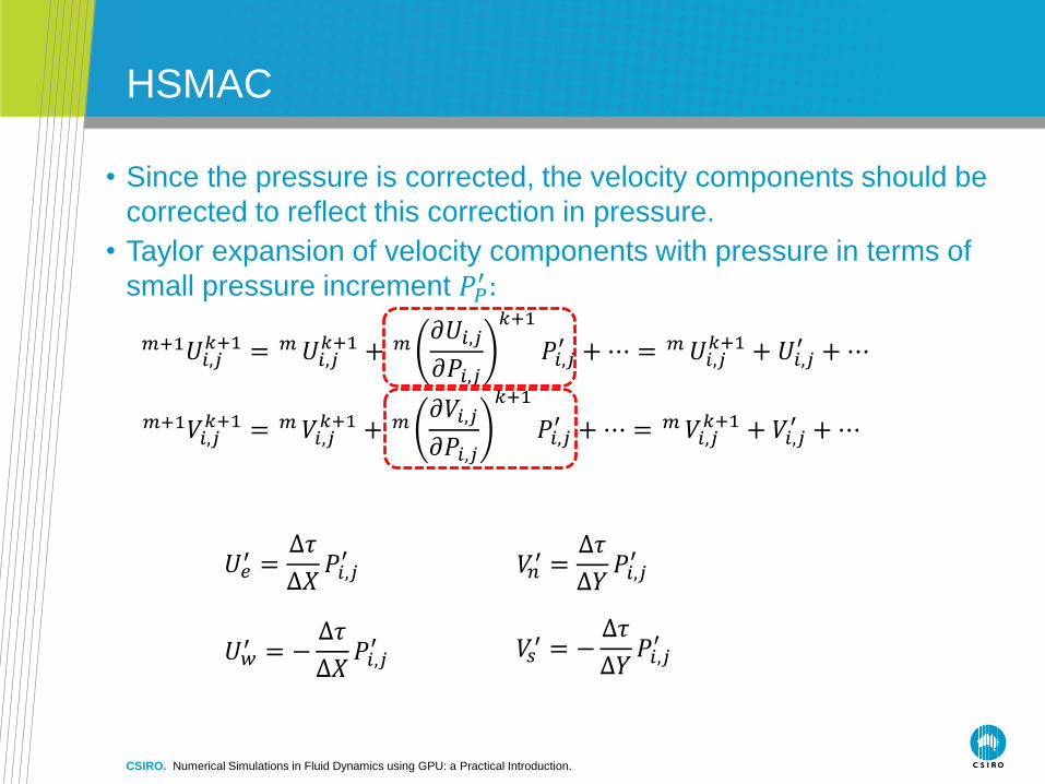
HSMAC
• Since the pressure is corrected, the velocity components should be
corrected to reflect this correction in pressure.
CSIRO. Numerical Simulations in Fluid Dynamics using GPU: a Practical Introduction.
• Taylor expansion of velocity components with pressure in terms of
small pressure increment 𝑃𝑃′ :
𝑚+1𝑈𝑖,𝑗𝑘+1 = 𝑚𝑈𝑖,𝑗
𝑘+1 + 𝑚𝜕𝑈𝑖,𝑗
𝜕𝑃𝑖,𝑗
𝑘+1
𝑃𝑖,𝑗′ +⋯ = 𝑚𝑈𝑖,𝑗
𝑘+1 + 𝑈𝑖,𝑗′ +⋯
𝑚+1𝑉𝑖,𝑗𝑘+1 = 𝑚 𝑉𝑖,𝑗
𝑘+1 + 𝑚𝜕𝑉𝑖,𝑗
𝜕𝑃𝑖,𝑗
𝑘+1
𝑃𝑖,𝑗′ +⋯ = 𝑚 𝑉𝑖,𝑗
𝑘+1 + 𝑉𝑖,𝑗′ +⋯
𝑈𝑒′ =
∆𝜏
∆𝑋𝑃𝑖,𝑗′ 𝑉𝑛
′ =∆𝜏
∆𝑌𝑃𝑖,𝑗′
𝑈𝑤′ = −
∆𝜏
∆𝑋𝑃𝑖,𝑗′ 𝑉𝑠
′ = −∆𝜏
∆𝑌𝑃𝑖,𝑗′
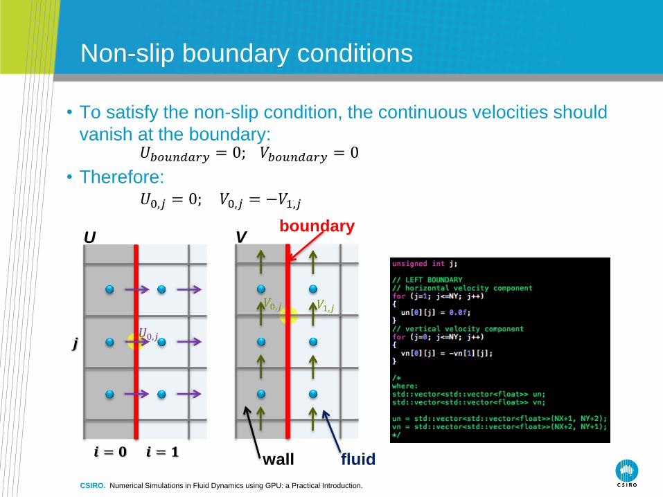
Non-slip boundary conditions
CSIRO. Numerical Simulations in Fluid Dynamics using GPU: a Practical Introduction.
fluid
boundary
wall
• To satisfy the non-slip condition, the continuous velocities should
vanish at the boundary:
U V
𝑈𝑏𝑜𝑢𝑛𝑑𝑎𝑟𝑦 = 0; 𝑉𝑏𝑜𝑢𝑛𝑑𝑎𝑟𝑦 = 0
• Therefore:
𝒊 = 𝟎 𝒊 = 𝟏
𝑈0,𝑗 = 0; 𝑉0,𝑗 = −𝑉1,𝑗
𝒋 𝑈0,𝑗
𝑉0,𝑗 𝑉1,𝑗

Free-slip boundary conditions
CSIRO. Numerical Simulations in Fluid Dynamics using GPU: a Practical Introduction.
fluid
boundary
wall
• The velocity component normal to boundary and normal derivative of
velocity component tangent to boundary should vanish:
U V
𝑈𝑏𝑜𝑢𝑛𝑑𝑎𝑟𝑦 = 0; 𝜕𝑉 𝜕𝑛 𝑏𝑜𝑢𝑛𝑑𝑎𝑟𝑦 = 0
• Therefore:
𝒊 = 𝟎 𝒊 = 𝟏
𝑈0,𝑗 = 0; 𝑉0,𝑗 = 𝑉1,𝑗
𝒋 𝑈0,𝑗
𝑉0,𝑗 𝑉1,𝑗

Case 1: Lid Driven Cavity
• Used as a validation case for new codes (same here?).
• Fluid is contained in a square cavity with three rigid walls (bottom, left and
right) and one moving wall (top).
CSIRO. Numerical Simulations in Fluid Dynamics using GPU: a Practical Introduction.
𝜕𝑈
𝜕𝜏+ 𝑈
𝜕𝑈
𝜕𝑋+ 𝑉
𝜕𝑈
𝜕𝑌= −
𝜕𝑃
𝜕𝑋+
1
𝑅𝑒
𝜕2𝑈
𝜕𝑋2+𝜕2𝑈
𝜕𝑌2
𝜕𝑉
𝜕𝜏+ 𝑈
𝜕𝑉
𝜕𝑋+ 𝑉
𝜕𝑉
𝜕𝑌= −
𝜕𝑃
𝜕𝑌+
1
𝑅𝑒
𝜕2𝑉
𝜕𝑋2+𝜕2𝑉
𝜕𝑌2
𝜕𝑈
𝜕𝑋+𝜕𝑉
𝜕𝑌= 0
• Reynolds number is a non dimensional parameter that
measure of the ratio of inertial forces to viscous forces:
𝑅𝑒 =
𝑖𝑛𝑒𝑟𝑡𝑖𝑎𝑙 𝑓𝑜𝑟𝑐𝑒
𝑣𝑖𝑠𝑐𝑜𝑢𝑠 𝑓𝑜𝑟𝑐𝑒=
𝑈𝐿
𝑣
Ve
locity
field

Case 1: Lid Driven Cavity
Re = 100 Re = 400 Re = 1000
Driven Cavity Test at Re = 1000
-0.7
-0.5
-0.3
-0.1
0.1
0.3
0.5
0.7
0.9
1.1
0 0.1 0.2 0.3 0.4 0.5 0.6 0.7 0.8 0.9 1
x and y location (respectively)
v a
nd
u v
elo
cit
y c
om
po
ne
nts
(re
sp
ec
tiv
ely
)
u- along y=0.5 (Ghia)
u- along y=0.5 (my code)
v- along x=0.5 (my code)
v- along x=0.5 (Ghia)
v- velocity component along y=0.5
u- velocity component along x=0.5
Re = 1000
str
eam
fu
nctio
n
CSIRO. Numerical Simulations in Fluid Dynamics using GPU: a Practical Introduction.
Ve
locity
field
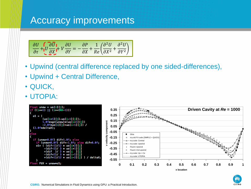
Accuracy improvements
𝜕𝑈
𝜕𝜏+ 𝑈
𝜕𝑈
𝜕𝑋+ 𝑉
𝜕𝑈
𝜕𝑌= −
𝜕𝑃
𝜕𝑋+
1
𝑅𝑒
𝜕2𝑈
𝜕𝑋2+𝜕2𝑈
𝜕𝑌2
• Upwind (central difference replaced by one sided-differences),
• Upwind + Central Difference,
• QUICK,
Driven Cavity Test at Re = 1000
-0.55
-0.45
-0.35
-0.25
-0.15
-0.05
0.05
0.15
0.25
0.35
0 0.1 0.2 0.3 0.4 0.5 0.6 0.7 0.8 0.9 1
x location
v v
elo
cit
y c
om
po
ne
nt
Ghia
my old FV code (SIMPLE + QUICK)
my code: Central
my code: Upwind
Fluent: Upwind
Fluent: 2nd upwind
my code: Up + Ce
my code: UTOPIA
Driven Cavity at Re = 1000
• UTOPIA:
CSIRO. Numerical Simulations in Fluid Dynamics using GPU: a Practical Introduction.

Case 2: Natural Convection
• Governing equations:
CSIRO. Numerical Simulations in Fluid Dynamics using GPU: a Practical Introduction.
Prandtl number describes the relative strength of the
diffusion of momentum to that of heat.
Rayleigh number expresses the ratio of the buoyancy
forces to viscous forces.
𝜕𝑈
𝜕𝜏+ 𝑈
𝜕𝑈
𝜕𝑋+ 𝑉
𝜕𝑈
𝜕𝑌= −
𝜕𝑃
𝜕𝑋+ 𝑃𝑟
𝜕2𝑈
𝜕𝑋2+𝜕2𝑈
𝜕𝑌2
𝜕𝑉
𝜕𝜏+ 𝑈
𝜕𝑉
𝜕𝑋+ 𝑉
𝜕𝑉
𝜕𝑌= −
𝜕𝑃
𝜕𝑌+ 𝑃𝑟
𝜕2𝑉
𝜕𝑋2+𝜕2𝑉
𝜕𝑌2+ 𝑅𝑎𝑃𝑟𝜃
𝜕𝑈
𝜕𝑋+𝜕𝑉
𝜕𝑌= 0
𝜕𝜃
𝜕𝜏+ 𝑈
𝜕𝜃
𝜕𝑋+ 𝑉
𝜕𝜃
𝜕𝑌=
𝜕2𝜃
𝜕𝑋2+𝜕2𝜃
𝜕𝑌2
• Characteristic non dimensional variables:
Conv. if Dr 0
𝑅𝑎 =𝑔𝛽(𝜃ℎ − 𝜃𝑐)𝑙
3
𝛼𝜈
𝑃𝑟 =𝜈
𝛼
𝜃ℎ 𝜃𝐶
𝜕𝜃
𝜕𝑌= 0
𝜕𝜃
𝜕𝑌= 0
𝑈 = 𝑉 = 0 on all walls
Temperature (TLC)

Case 2: Natural Convection
𝑹𝒂 = 𝟏𝟎𝟒, 𝑷𝒓 = 𝟎. 𝟕𝟏
𝑹𝒂 = 𝟏𝟎𝟔, 𝑷𝒓 = 𝟎. 𝟕𝟏
CSIRO. Numerical Simulations in Fluid Dynamics using GPU: a Practical Introduction.
128x128
Max of V- at Y = 0.5:
HSMAC: 19.56 at x = 0.1114 err 0.2906%
Benchmark: 19.617 at x = 0.119
Max of U- at X = 0.5:
HSMAC: 16.108 at y = 0.8324 err 0.4327%
Benchmark: 16.178 at y = 0.823
Max of V- at Y = 0.5:
HSMAC: 219.5 at x = 0.03622 err 0.0638%
Benchmark: 219.36 at x = 0.03790
Max of U- at X = 0.5:
HSMAC: 64.492 at y = 0.85 err 0.2135%
Benchmark: 64.630 at y = 0.850
𝑅𝑎 = 104
𝑅𝑎 = 106
• Variables to be compared: temperature and velocity profiles, stream function, Nusselt number
Te
mp
era
ture
T
em
pe
ratu
re
Velo
city
Stre
am
functio
n
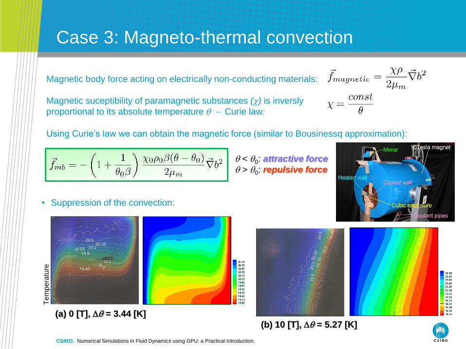
Case 3: Magneto-thermal convection
CSIRO. Numerical Simulations in Fluid Dynamics using GPU: a Practical Introduction.
Magnetic body force acting on electrically non-conducting materials:
Magnetic suceptibility of paramagnetic substances () is inversly
proportional to its absolute temperature q - Curie law:
Using Curie’s law we can obtain the magnetic force (similar to Bousinessq approximation):
q < q0: attractive force
q > q0: repulsive force
• Suppression of the convection:
(a) 0 [T], Dq = 3.44 [K]
(b) 10 [T], Dq = 5.27 [K]
Te
mp
era
ture
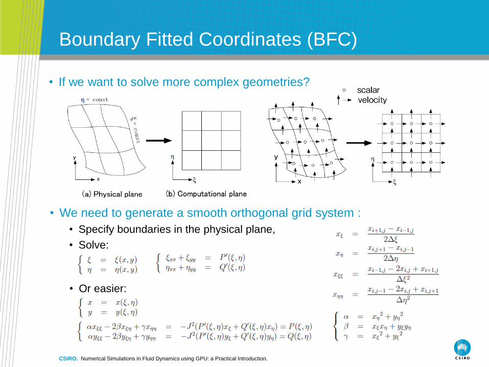
Boundary Fitted Coordinates (BFC)
CSIRO. Numerical Simulations in Fluid Dynamics using GPU: a Practical Introduction.
• If we want to solve more complex geometries?
• We need to generate a smooth orthogonal grid system :
• Specify boundaries in the physical plane,
• Solve:
• Or easier:

Boundary Fitted Coordinates (BFC)
• Sample grids
CSIRO. Numerical Simulations in Fluid Dynamics using GPU: a Practical Introduction.
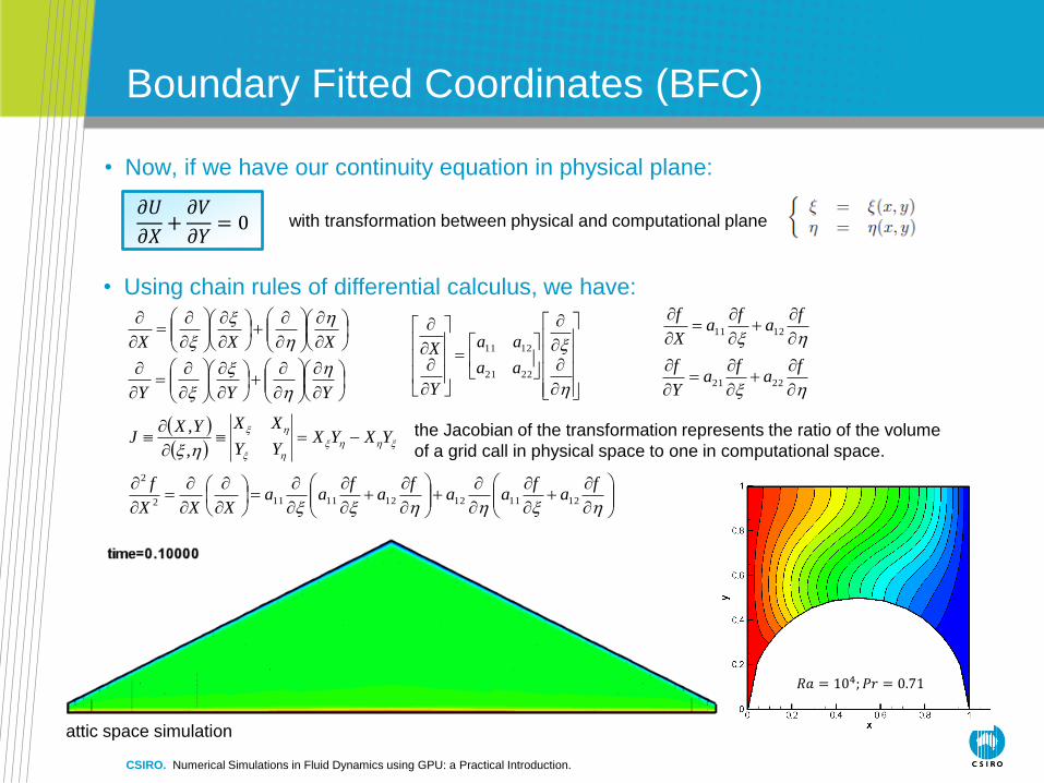
Boundary Fitted Coordinates (BFC)
CSIRO. Numerical Simulations in Fluid Dynamics using GPU: a Practical Introduction.
𝑅𝑎 = 104; 𝑃𝑟 = 0.71
• Now, if we have our continuity equation in physical plane:
𝜕𝑈
𝜕𝑋+𝜕𝑉
𝜕𝑌= 0
XXX
YYY
2221
1211
aa
aa
Y
X
with transformation between physical and computational plane
• Using chain rules of differential calculus, we have:
YXYX
YY
XXYXJ -
,
,
fa
fa
X
f1211
fa
fa
Y
f2221
the Jacobian of the transformation represents the ratio of the volume
of a grid call in physical space to one in computational space.
fa
faa
fa
faa
XXX
f1211121211112
2
attic space simulation
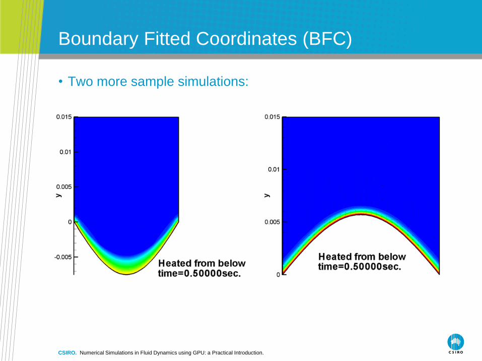
Boundary Fitted Coordinates (BFC)
• Two more sample simulations:
CSIRO. Numerical Simulations in Fluid Dynamics using GPU: a Practical Introduction.

Applications: scaling analysis
• Used to predict behaviour of the fluid flow for different cases.
• Approach: by comparing terms of governing equations.
CSIRO. Numerical Simulations in Fluid Dynamics using GPU: a Practical Introduction.
• Transient flow:
HSMAC on GPU
CSIRO. Numerical Simulations in Fluid Dynamics using GPU: a Practical Introduction.

OpenCL™
• OpenCL (Open Compute Language): an open, royalty-free standard
for parallel programming of heterogeneous systems that include
multi-core processors (CPUs), graphics processing units (GPUs),
and other accelerators such as Cell and digital signal processors
(DSPs).
• OpenCL has complex platform and device management model that
reflects its support for multi-platform and multi-vendor portability.
• Uniform programming environment to write efficient, portable code
for HPC servers, desktop computer systems and handheld devices.
• The standard includes an API for coordinating execution between
devices and a cross-platform parallel programming language.
• Initiated by Apple (now specification editor) and developed by the
Khronos Group.
CSIRO. Numerical Simulations in Fluid Dynamics using GPU: a Practical Introduction.
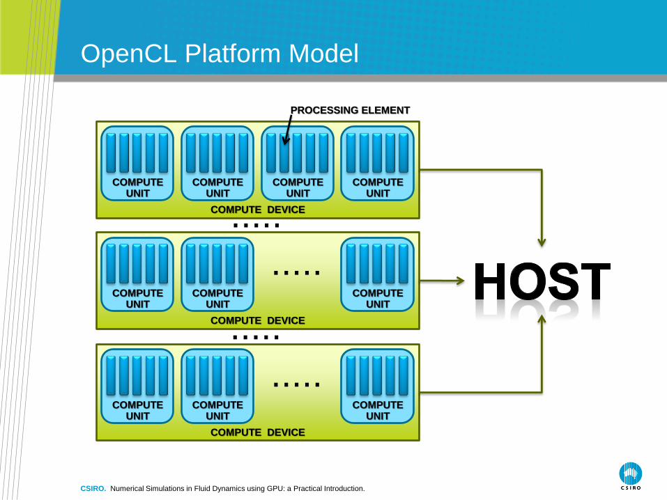
OpenCL Platform Model
CSIRO. Numerical Simulations in Fluid Dynamics using GPU: a Practical Introduction.
COMPUTE UNIT
COMPUTE UNIT
COMPUTE UNIT
COMPUTE UNIT
COMPUTE DEVICE
PROCESSING ELEMENT
COMPUTE UNIT
COMPUTE UNIT
COMPUTE UNIT
COMPUTE DEVICE
.....
COMPUTE UNIT
COMPUTE UNIT
COMPUTE UNIT
COMPUTE DEVICE
.....
.....
.....

Tested GPUs
• GPU Features…
CSIRO. Numerical Simulations in Fluid Dynamics using GPU: a Practical Introduction.
GT 330M QFX4600 QFX4800 460GTX S2050
Streaming Multiprocessors (SM) 6 12 24 7 14
Streaming Processors (SP) / Cores 48 96 192 224 448
Registers per SM 16K 8K 16K 32KB 32KB
Shared Memory per SM 16KB 16KB 16KB 48KB 48KB
Processor Clock [MHz] 990 1200 1204 810 1147
Work item size 512/512/64 512/512/64 512/512/64 1024/1024/64 1024/1024/64
Work group size 512 512 512 1024 1024
CUDA Compute Capability 1.2 1.0 1.3 2.x 2.x
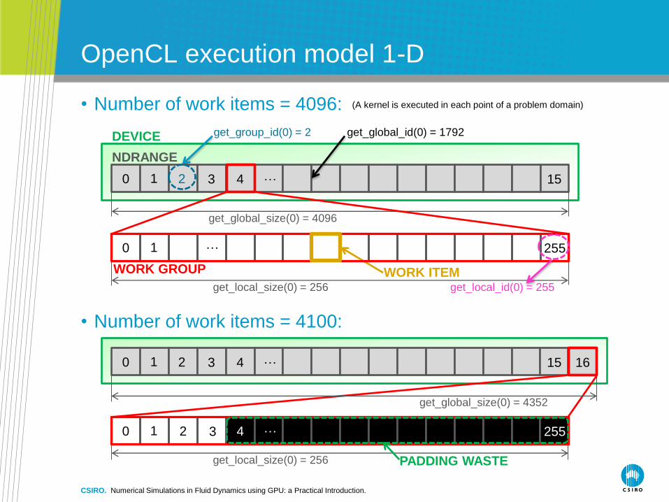
OpenCL execution model 1-D
• Number of work items = 4096:
NDRANGE
DEVICE get_group_id(0) = 2
0 1 2 15
get_global_size(0) = 4096
get_local_size(0) = 256
3 … 4
get_global_id(0) = 1792
WORK GROUP WORK ITEM get_local_id(0) = 255
0 1 … 255
• Number of work items = 4100:
0 1 2 15
get_local_size(0) = 256
3 … 4
0 1 255
16
2 3 … 4
PADDING WASTE
get_global_size(0) = 4352
CSIRO. Numerical Simulations in Fluid Dynamics using GPU: a Practical Introduction.
(A kernel is executed in each point of a problem domain)
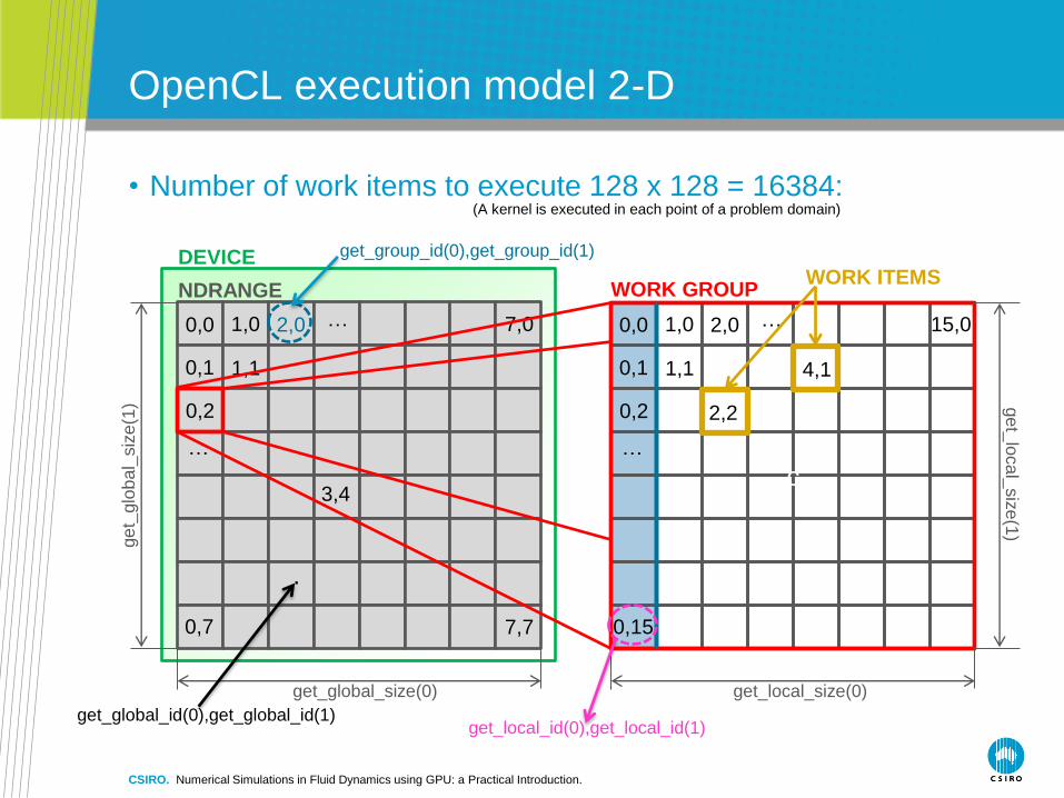
OpenCL execution model 2-D
• Number of work items to execute 128 x 128 = 16384:
NDRANGE
DEVICE
0,0 1,0 2,0
0,1
0,2
1,1
…
…
7,0
7,7 0,7
3,4
0,0 1,0 2,0
0,1
0,2
1,1
…
…
15,0
0,15
c
WORK GROUP WORK ITEMS
CSIRO. Numerical Simulations in Fluid Dynamics using GPU: a Practical Introduction.
2,2
4,1
get_global_size(0)
ge
t_glo
bal_
siz
e(1
) ge
t_lo
ca
l_siz
e(1
)
get_local_size(0)
get_group_id(0),get_group_id(1)
get_local_id(0),get_local_id(1) get_global_id(0),get_global_id(1)
.
(A kernel is executed in each point of a problem domain)

HOST OUTER LOOP
Flow Chart of the OpenCL Fluid Solver
START
Read Configuration
Allocate Memory for Flow
Field Tables
Apply Boundary
Conditions (BC)
Calculate Tentative
Velocities (U, V)
Calculate Pressure
Correction
Correct Pressure and
Velocity Fields, Apply BC
Converged? NO
Calculate Energy
Equation (if required)
YES Final time
achieved?
Advance All Flow Tables
and Increase Time
NO
Save Results: Flow
Fields, etc...
FINISH
YES
HOST INNER LOOP
CSIRO. Numerical Simulations in Fluid Dynamics using GPU: a Practical Introduction.
Get OpenCL Platform,
Initialize Device, Create
Context, Create
Command Queue
Create OCL Memory
Buffers
Create OCL Program,
Create Kernels and Set
Kernel Arguments
Setup Boundary Flags
Copy Host Memory
Buffers to GPU Buffers
krnl_bc_u krnl_bc_v krnl_bc_p
krnl_momentum_u krnl_momentum_v
krnl_pressure_velocity_correction
krnl_bc_u krnl_bc_v krnl_bc_p
krnl_energy
krnl_advance_u krnl_advance_v
Copy GPU Buffers to
Host Memory Buffers
Release Command
Queue, Context, Kernels,
Programs, Memory
Visualisation
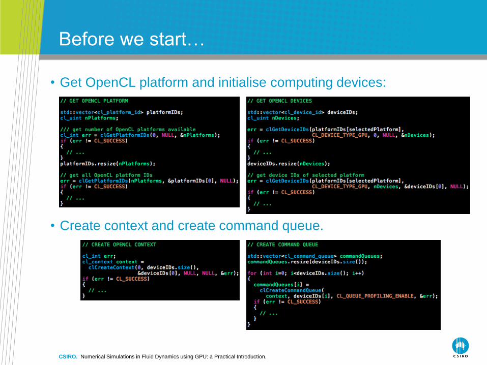
Before we start…
• Get OpenCL platform and initialise computing devices:
• Create context and create command queue.
CSIRO. Numerical Simulations in Fluid Dynamics using GPU: a Practical Introduction.
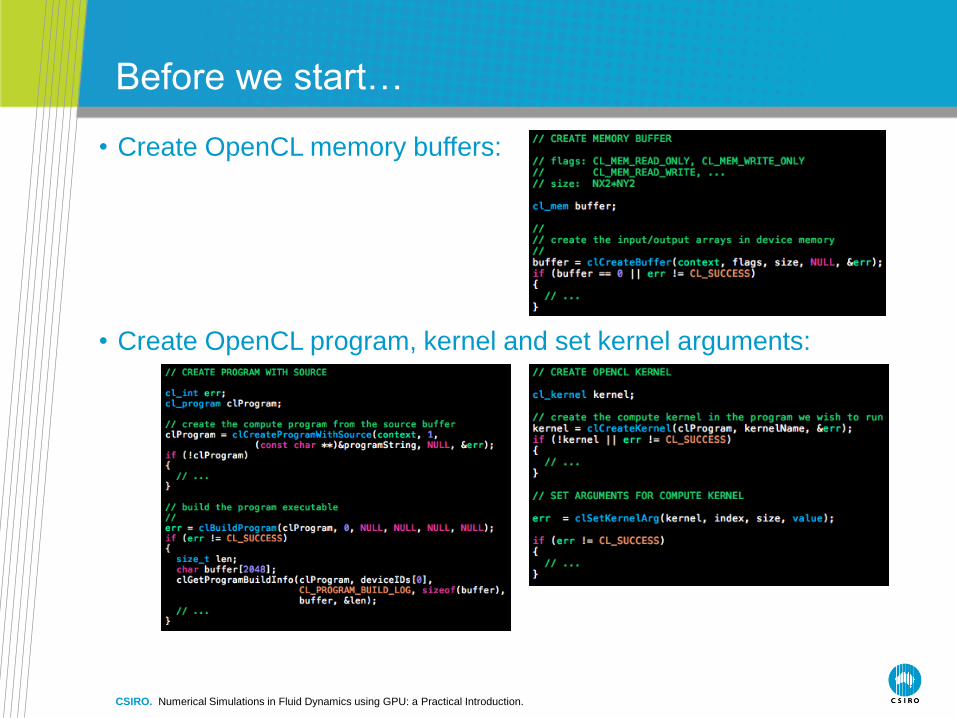
Before we start…
• Create OpenCL program, kernel and set kernel arguments:
• Create OpenCL memory buffers:
CSIRO. Numerical Simulations in Fluid Dynamics using GPU: a Practical Introduction.

OpenCL Class Diagram
CSIRO. Numerical Simulations in Fluid Dynamics using GPU: a Practical Introduction.
• UML class diagram of OpenCL: relationships between classes,
• Solid diamonds (aggregations), inheritance (open arrowhead),
cardinality: * many, 1 one and only one, 0..1 optionally one, 1..* one
or more.
Reconstructed from Figure 2.1 of the Khronos OpenCL Specification.

ComputeEngine Class
CSIRO. Numerical Simulations in Fluid Dynamics using GPU: a Practical Introduction.
• Example:
• Kernels call:

Boundary Conditions on GPU
• Setup boundary conditions
• Create “ghost” cells for velocity, pressure, temperature and
concentration fields.
• Below: ghost cells to assist scalar computations.
CSIRO. Numerical Simulations in Fluid Dynamics using GPU: a Practical Introduction.
𝒊 = 𝟎 𝒊 = 𝟏 𝒊 = 𝟐 𝒊 = 𝟑 𝒊 = 𝟒 𝒊 = 𝟔 𝒊 = 𝟕
𝒋 = 𝟒
𝒋 = 𝟑
𝒋 = 𝟐
𝒋 = 𝟏
𝒋 = 𝟎
𝒊 = 𝟓
𝒈𝒉𝒐𝒔𝒕 = 𝟏
𝒈𝒉𝒐𝒔𝒕 = 𝟑
𝒈𝒉𝒐𝒔𝒕 = 𝟒
𝒈𝒉𝒐𝒔𝒕 = 𝟐
𝒅𝒐𝒎𝒂𝒊𝒏
𝑵𝑿 = 𝟔; 𝑵𝒀 = 𝟑
𝑵𝑿𝟐 = 𝟖; 𝑵𝒀𝟐 = 𝟓

Boundary conditions on GPU
CSIRO. Numerical Simulations in Fluid Dynamics using GPU: a Practical Introduction.
𝟎 𝟏 𝟐 𝟑 𝟒 𝟓 𝟔 𝟕
𝟒
𝟑
𝟐
𝟏
𝟎
𝟎 𝟏 𝟐 𝟑 𝟒 𝟓 𝟔 𝟕
𝟏
𝟐
𝟑
𝟒
−𝟏
• Velocity boundary conditions
• For simplicity, the memory buffer for vectors is of the same size as
for scalar variables.
• For horizontal velocity component there is one column of waste.
• For vertical velocity components there is one row of waste.
𝑵𝑿 = 𝟔; 𝑵𝒀 = 𝟑
𝑵𝑿𝟐 = 𝟖; 𝑵𝒀𝟐 = 𝟓
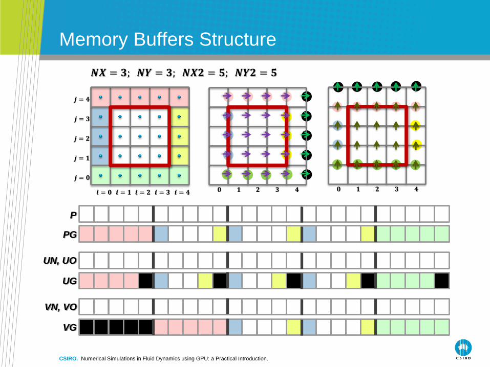
Memory Buffers Structure
𝟎 𝟏 𝟐 𝟑 𝟒 𝟎 𝟏 𝟐 𝟑 𝟒 𝒊 = 𝟎 𝒊 = 𝟏 𝒊 = 𝟐 𝒊 = 𝟑 𝒊 = 𝟒
𝒋 = 𝟒
𝒋 = 𝟑
𝒋 = 𝟐
𝒋 = 𝟏
𝒋 = 𝟎
𝑵𝑿 = 𝟑; 𝑵𝒀 = 𝟑; 𝑵𝑿𝟐 = 𝟓; 𝑵𝒀𝟐 = 𝟓
P
PG
UN, UO
UG
VN, VO
VG
CSIRO. Numerical Simulations in Fluid Dynamics using GPU: a Practical Introduction.

Apply boundary conditions
𝟎 𝟏 𝟐 𝟑 𝟒 𝟎 𝟏 𝟐 𝟑 𝟒 𝒊 = 𝟎 𝒊 = 𝟏 𝒊 = 𝟐 𝒊 = 𝟑 𝒊 = 𝟒
𝒋 = 𝟒
𝒋 = 𝟑
𝒋 = 𝟐
𝒋 = 𝟏
𝒋 = 𝟎
CSIRO. Numerical Simulations in Fluid Dynamics using GPU: a Practical Introduction.

Calculate tentative velocity component U
CSIRO. Numerical Simulations in Fluid Dynamics using GPU: a Practical Introduction.
𝜕𝑈
𝜕𝜏+ 𝑈
𝜕𝑈
𝜕𝑋+ 𝑉
𝜕𝑈
𝜕𝑌= −𝐴
𝜕𝑃
𝜕𝑋+ 𝐵
𝜕2𝑈
𝜕𝑋2 +𝜕2𝑈
𝜕𝑌2
𝑈𝑖,𝑗𝑘+1=
𝑈𝑖,𝑗𝑘 + ∆𝜏 −𝐹𝑈𝑋 − 𝐹𝑈𝑌 − 𝑃𝑅𝐸𝑆𝑆𝑈 + 𝐷𝐼𝐹𝐹𝑈
• From X- momentum equation
𝑃 𝐸 𝑊
𝑁
𝑆
𝐸𝑁
𝐸𝑆
𝑊𝑁
𝑊𝑆
𝑒 𝑤 𝑒𝑒
𝑒𝑛
𝑒𝑠
𝑤𝑛
𝑤𝑠
𝑛
𝑠
𝑛𝑛
𝑤𝑛
𝑤𝑠
𝑒𝑛
𝑒𝑠
𝑤𝑛𝑛 𝑒𝑛𝑛
𝑒𝑒𝑛
𝑒𝑒𝑠
∆𝑌
∆𝑋

𝑃 𝐸 𝑊
𝑁
𝑆
𝐸𝑁
𝐸𝑆
𝑊𝑁
𝑊𝑆
𝑒 𝑤 𝑒𝑒
𝑒𝑛
𝑒𝑠
𝑤𝑛
𝑤𝑠
𝑛
𝑠
𝑛𝑛
𝑤𝑛
𝑤𝑠
𝑒𝑛
𝑒𝑠
𝑤𝑛𝑛 𝑒𝑛𝑛
𝑒𝑒𝑛
𝑒𝑒𝑠
∆𝑌
∆𝑋
𝑉𝑖,𝑗𝑘+1 =
𝑉𝑖,𝑗𝑘 + ∆𝜏 −𝐹𝑉𝑋 − 𝐹𝑉𝑌 − 𝑃𝑅𝐸𝑆𝑆𝑉 + 𝐷𝐼𝐹𝐹𝑉
𝜕𝑉
𝜕𝜏+ 𝑈
𝜕𝑉
𝜕𝑋+ 𝑉
𝜕𝑉
𝜕𝑌= −𝐴
𝜕𝑃
𝜕𝑌+ 𝐵
𝜕2𝑉
𝜕𝑋2 +𝜕2𝑉
𝜕𝑌2
Calculate tentative velocity component V
CSIRO. Numerical Simulations in Fluid Dynamics using GPU: a Practical Introduction.
• From X- momentum equation

Pressure and velocity corrections
𝐷𝑚𝑖,𝑗𝑘+1 =
𝑈𝑚𝑖,𝑗𝑘+1 − 𝑈𝑚
𝑖−1,𝑗𝑘+1
∆𝑋+
𝑉𝑚𝑖,𝑗𝑘+1 − 𝑉𝑚
𝑖,𝑗−1𝑘+1
∆𝑌= 𝐷
𝑚𝜕𝐷𝑖,𝑗
𝜕𝑃𝑖,𝑗
𝑘+1
=
∆𝜏1
∆𝑋
1
∆𝑋+
1
∆𝑋+
1
∆𝑌
1
∆𝑌+
1
∆𝑌= 𝐷𝐸𝐿
𝑈𝑒′ =
∆𝜏
∆𝑋𝑃𝑖,𝑗′
𝑉𝑛′ =
∆𝜏
∆𝑌𝑃𝑖,𝑗′
𝑈𝑤′ = −
∆𝜏
∆𝑋𝑃𝑖,𝑗′
𝑉𝑠′ = −
∆𝜏
∆𝑌𝑃𝑖,𝑗′
𝑃𝑃′ = −
𝐷
𝐷𝐸𝐿
𝑃 𝐸 𝑊
𝑁
𝑆
𝐸𝑁
𝐸𝑆
𝑊𝑁
𝑊𝑆
𝑒 𝑤 𝑒𝑒
𝑒𝑛
𝑒𝑠
𝑤𝑛
𝑤𝑠
𝑛
𝑠
𝑛𝑛
𝑤𝑛
𝑤𝑠
𝑒𝑛
𝑒𝑠
𝑤𝑛𝑛 𝑒𝑛𝑛
𝑒𝑒𝑛
𝑒𝑒𝑠
∆𝑌
∆𝑋
CSIRO. Numerical Simulations in Fluid Dynamics using GPU: a Practical Introduction.

Advance flow tables
• Advance velocity:
CSIRO. Numerical Simulations in Fluid Dynamics using GPU: a Practical Introduction.
• And for instance, this can be optimised explicitly:

0
500
1000
1500
2000
2500
0 64 128 192 256 320
Tim
e [
s]
Number of cells (K)
S2050
GT 330M
Measures for Execution Speedup
• Driven Cavity
5
10
15
20
25
30
35
32 64 96 128
Sp
eed
up
X (
GP
U/C
PU
)
Grid Size
GPU/CPU
GeForce GT 330M
CSIRO. Numerical Simulations in Fluid Dynamics using GPU: a Practical Introduction.
• Natural Convection
CPU: Intel Core i7 2.66Ghz
~7-9 x
Grid size GT 130M S2050
32 x 32 40.64 s 8.17 s
64 x 64 83.54 s 11.37 s
128 x 128 218.27 s 24.14 s
256 x 256 678.58 s 93.61 s
512 x 512 2477.87 s 353.72 s
Execution times:

CSIRO GPU Cluster
CSIRO. Numerical Simulations in Fluid Dynamics using GPU: a Practical Introduction.

CSIRO GPU Cluster Launch (25 November 2009)
CSIRO. Numerical Simulations in Fluid Dynamics using GPU: a Practical Introduction.

CSIRO GPU Cluster Configuration
GPU Cluster Configuration
The new CSIRO GPU cluster will deliver up
to 264 plus Teraflops of single precision
computing performance and will consist of:
•128 Dual Xeon E5462 Compute Nodes
(i.e. a total of 1024 2.8GHz compute cores)
with 16 or 32GB of RAM, 500GB SATA
storage and DDR InfiniBand interconnect
•64 Tesla S250’s (256 GPUs with a total of
114,688 CUDA processor cores)
•144 port DDR InfiniBand Switch
•80 Terabyte Hitachi NAS file system.
CSIRO. Numerical Simulations in Fluid Dynamics using GPU: a Practical Introduction.

CSIRO GPU Cluster
Linux and Windows
Production
Environment
Linux and Windows
Test & Training
Environment
Linux and Windows
Management
Nodes
Currently
1024 CPU cores
64 Tesla s1070’s
(256 GPUs with
61,440 CUDA cores)

CSIRO GPU Cluster
CSIRO. Numerical Simulations in Fluid Dynamics using GPU: a Practical Introduction.
NVIDIA CUDA Research Center
• CSIRO, in recognition of its leadership in massively parallel computing, is an inaugural member of the NVIDIA CUDA Research Center program
• Institutions identified as CUDA Research Centers are doing world-changing research by leveraging CUDA and NVIDIA GPUs. CUDA Research Centers and PIs:
• CSIRO (PI: John Taylor)
• ICHEC (PI: Gilles Civario)
• Johns Hopkins University (PI: Alex Szalay)
• Mass General-Harvard Medical School (PI: Homer Pien)
• Nanyang University (PI: Bertil Schmidt)
• SINTEF (PI: Trond Runar Hagan)
• Technical University of Ostrava (PI: Eduard Sojka)
CSIRO. Numerical Simulations in Fluid Dynamics using GPU: a Practical Introduction.
CSIRO Computational and Simulation Sciences
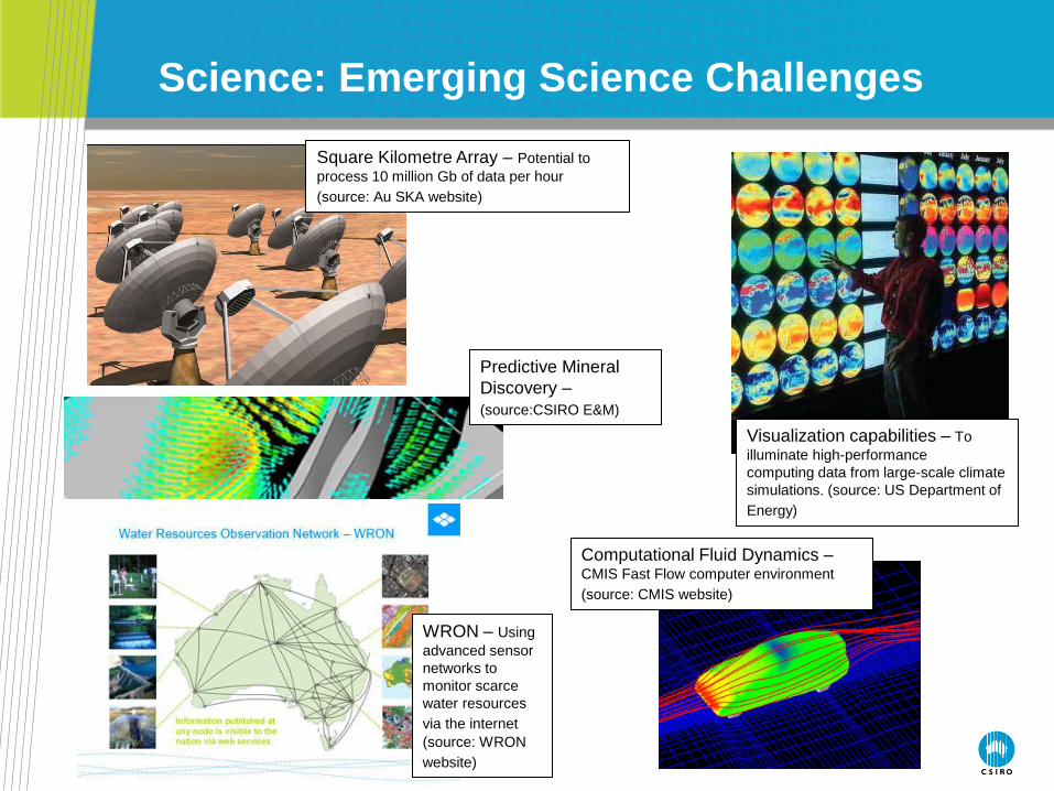
Science: Emerging Science Challenges
Square Kilometre Array – Potential to
process 10 million Gb of data per hour
(source: Au SKA website)
Visualization capabilities – To
illuminate high-performance
computing data from large-scale climate
simulations. (source: US Department of
Energy)
Computational Fluid Dynamics – CMIS Fast Flow computer environment
(source: CMIS website)
Predictive Mineral
Discovery –
(source:CSIRO E&M)
WRON – Using
advanced sensor
networks to
monitor scarce
water resources
via the internet (source: WRON
website)
Summary
• CFD does not need to be scary !!!
• We used the following approach:
• Equations Discretisation Implementation Verification
Results Transfer CPU code to GPU code Verification
Results.
• Methods presented:
• Finite Difference Method (for discretisation),
• HSMAC Method (for mutual iteration of pressure/velocity fields),
• BFC (for solving Navier-Stokes equations on complex geometry),
• Upwind and UTOPIA (for getting more stable and accurate results),
• OpenCL (for speeding-up computing process).
• The methodology presented, can be extended into 3D and
applied to compute different cases in real-time, e.g., smoke,
free surface flows, ventilation, turbulent flows, etc.
• Source-code to be released online.
CSIRO. Numerical Simulations in Fluid Dynamics using GPU: a Practical Introduction.


Contact Us
Phone: 1300 363 400 or +61 3 9545 2176
Email: [email protected] Web: www.csiro.au
Thank you… …
Earth Science and Resource Engineering
Dr Tomasz P Bednarz
3D Visualisation Engineer
Mining Automation
Phone: +61 429 153 274
Email: [email protected]
Web: www.csiro.au/org/CESRE.html
www.tomaszbednarz.com
Acknowledgments: Dr J.Taylor, C.Caris, Prof. H.Ozoe, Prof. H.Hirano, Prof. T.Tagawa, Prof. J.C.Patterson,
Prof. Chengwang Lei, Prof. J.S.Szmyd, Dr P.Cleary, Dr M.Rudman, Dr J.Ralston,
Dr L.Domanski, Dr J.Malos, J.Craig, Dr S.Zawlodzka-Bednarz


