July 2007Jan Tommy Gravdahl, ITKErik Stiklestad, Aker Verdal
Master of Science in Engineering CyberneticsSubmission date:Supervisor:Co-supervisor:
Norwegian University of Science and TechnologyDepartment of Engineering Cybernetics
Numerical Modelling and ModelReduction of Heat Flow in RoboticWelding
Mads Martinussen


Problem DescriptionThe topic of this thesis is to develop a numerical model of heat flow in robotic welding. Theultimate goal of the work is to apply the model to trajectory planning and speed control of thewelding robot, and thereby achieve better quality welds.
Sub tasks:1. Perform a literature study on robotic welding.2. Describe the heat flow problem in robotic welding using partial differential equations.3. Present the finite element method.4. Use the above methods to develop a numerical model of heat flow. Specifically, provide an estimate of the cooling time from 800 C to 500 C in the seam.5. Present a number of methods in model order reduction, with particular weight on proper orthogonal decomposition(POD).6. Perform model reduction of the numerical model using POD, and do an evaluation of the reduced model's general performance.7. Perform experiments in temperature measurements of welding using an infrared camera. More specifically, there will be performed an evaluation on weather or not this method may be used as a decision parameter in an automated system.
Assignment given: 28. February 2007Supervisor: Jan Tommy Gravdahl, ITK

Preface
This master’s thesis is a compulsory part of the fifth year masters study of engineering
cybernetics at NTNU. The project was done in cooperation with Aker Kværner Verdal
A/S.
Through the term at which the thesis has been done, I have learnt a lot about the com-
plex nature of welding and the relating fields of study. At the initial point of the project,
the framework was not very well defined. This resulted in a lot of work in identifying the
nature of the problem, and finding out how to approach it. This resulted in many hours of
frustration. When later having similar large projects like this, there will be put more work
in finding a proper frame-work.
I would like to thank my supervisor, Jan Tommy Gravdahl, for great support through-
out the thesis. I would also like to thank Erik Stiklestad at Aker kværner Verdal A/S for
making this project possible. He supported me with relevant information regarding the
projects nature. He made the welding experiments with the IR-camera possible, providing
equipment and time on the robot gantry. I would also like to thank Øystein Grong for
constructive critics of my work, and giving me guidance on how to approach problems
related to thermal analysis of welds. A thank you should also be directed toward Svein
Hovland for giving me a crash course in model reduction. I would never have been able to
complete the work without his help. Last but not least, my fellow students at GG48 have
been a great support throughout the entire period, giving me encouraging feedback all the
way.
Trondheim, July 18, 2007
Mads Martinussen
i

Abstract
This thesis is a case study of robotic welding, where the majority of the work has been
done on studying the complex nature of the partial differential equations governing the heat
distribution in steel plates. In order to get fundamental knowledge about welding and, in
principal concern, on the automated side of it, there has been done a general literature study
on robotic welding in Chapter 2. Here the major issues concerning welding are covered.
The topics covered are equipment used, parameters governing the process and sensors used
in automated systems. In Chapter 3, the partial differential equations are introduced, where
the basic assumptions in the case of welding are taken, and an analytical solution, valid for
thick plates in pseudo steady state is derived. This solution will later in the thesis be used as
a reference temperature distribution in order to validate the model made through numerical
modelling. The numerical model has been made in a software environment based on the
finite element method. As an introduction to this method, Chapter 4 goes through the
basic ideas behind the method, and introduces the weak form, a method for solving the
weighted integral statement. The basic procedure in making the model, obtaining a Δt8/5
and comparing the results with the reference model from Chapter 3, are covered in Chapter
6. In Chapter 5 the theory behind some model order reduction techniques are outlined.
The main focus will be put on Proper Orthogonal Decomposition. The theory is put into
practice in Chapter 7, where a reduced model is obtained through a number of steps based
on the model obtained in Chapter 6. As an introductionary study to future work on the full
automated system, experiments in online measurements of the temperature in the welded
specimen are done in Chapter 8. Discussions are done after each relevant chapter and
conclusions are drawn in Chapter 9.
Keywords: Robotic welding, welding equipment and parameters, heat flow modelling,
the finite element method, Δt8/5, model reduction, IR-thermography.
iii


Table of Contents
1 Introduction 1
2 A literature study in robotic welding theory 32.1 Welding equipment . . . . . . . . . . . . . . . . . . . . . . . . . . . . . 4
2.1.1 Power source . . . . . . . . . . . . . . . . . . . . . . . . . . . . 4
2.1.2 Electrode feed unit . . . . . . . . . . . . . . . . . . . . . . . . . 4
2.1.3 Welding torch . . . . . . . . . . . . . . . . . . . . . . . . . . . . 4
2.2 Process parameters . . . . . . . . . . . . . . . . . . . . . . . . . . . . . 5
2.2.1 Current . . . . . . . . . . . . . . . . . . . . . . . . . . . . . . . 5
2.2.2 Voltage . . . . . . . . . . . . . . . . . . . . . . . . . . . . . . . 5
2.2.3 Welding speed . . . . . . . . . . . . . . . . . . . . . . . . . . . 5
2.2.4 Electrode extension . . . . . . . . . . . . . . . . . . . . . . . . . 5
2.2.5 Shielding gas . . . . . . . . . . . . . . . . . . . . . . . . . . . . 6
2.2.6 Electrode diameter . . . . . . . . . . . . . . . . . . . . . . . . . 6
2.2.7 Welding Angle . . . . . . . . . . . . . . . . . . . . . . . . . . . 6
2.3 Welding sensors . . . . . . . . . . . . . . . . . . . . . . . . . . . . . . . 6
2.4 Sensors for technological parameters . . . . . . . . . . . . . . . . . . . . 7
2.4.1 Arc voltage . . . . . . . . . . . . . . . . . . . . . . . . . . . . . 7
2.4.2 Welding current . . . . . . . . . . . . . . . . . . . . . . . . . . . 7
2.4.3 Wire Feed Speed . . . . . . . . . . . . . . . . . . . . . . . . . . 7
2.5 Sensors for geometrical parameters . . . . . . . . . . . . . . . . . . . . . 7
2.5.1 Contact sensors . . . . . . . . . . . . . . . . . . . . . . . . . . . 7
2.5.2 Optical sensors . . . . . . . . . . . . . . . . . . . . . . . . . . . 8
2.5.3 Arc Sensors . . . . . . . . . . . . . . . . . . . . . . . . . . . . . 8
2.6 Sensors Detecting Temperature . . . . . . . . . . . . . . . . . . . . . . . 8
3 Heat flow modelling 113.1 The general heat flow equation . . . . . . . . . . . . . . . . . . . . . . . 11
3.2 Heat input and arc efficiency factor . . . . . . . . . . . . . . . . . . . . . 12
3.3 The thick plate solution . . . . . . . . . . . . . . . . . . . . . . . . . . . 12
3.4 Temperature decay rate . . . . . . . . . . . . . . . . . . . . . . . . . . . 15
4 The finite element method 174.1 The basic features of the method . . . . . . . . . . . . . . . . . . . . . . 18
4.2 The weighted integral and weak form formulations . . . . . . . . . . . . 18
v
4.2.1 The weighted integral statement . . . . . . . . . . . . . . . . . . 18
4.2.2 The weak form . . . . . . . . . . . . . . . . . . . . . . . . . . . 19
4.2.3 Summary . . . . . . . . . . . . . . . . . . . . . . . . . . . . . . 22
5 Model order reduction 235.1 Problem statement . . . . . . . . . . . . . . . . . . . . . . . . . . . . . 24
5.2 Proper orthogonal decomposition . . . . . . . . . . . . . . . . . . . . . . 24
5.3 Rational Krylov algorithms . . . . . . . . . . . . . . . . . . . . . . . . . 25
5.4 Fourier model reduction . . . . . . . . . . . . . . . . . . . . . . . . . . 26
5.5 Balanced realization and truncation . . . . . . . . . . . . . . . . . . . . . 28
6 Numerical modelling and analysis of heat flow in a single-pass butt weldingseam 296.1 Construction of the model . . . . . . . . . . . . . . . . . . . . . . . . . 29
6.2 Response analysis . . . . . . . . . . . . . . . . . . . . . . . . . . . . . . 30
6.2.1 Relation between Q and q0 . . . . . . . . . . . . . . . . . . . . . 30
6.2.2 Relevant Plots . . . . . . . . . . . . . . . . . . . . . . . . . . . 30
6.3 Discussion . . . . . . . . . . . . . . . . . . . . . . . . . . . . . . . . . . 32
7 Applying POD to the numerical FEM-model 397.1 Linearizing the model . . . . . . . . . . . . . . . . . . . . . . . . . . . . 39
7.2 Reducing the order of the model . . . . . . . . . . . . . . . . . . . . . . 43
7.2.1 Snapshot matrix from one simulation . . . . . . . . . . . . . . . 43
7.2.2 Snapshot matrix from several initial value simulations . . . . . . 43
7.2.3 Snapshot matrix from several simulations including input u . . . 48
7.2.4 Applying other inputs to the reduced model . . . . . . . . . . . . 48
7.3 Discussion and evaluation . . . . . . . . . . . . . . . . . . . . . . . . . . 53
8 Temperature experiments at Aker Kværner Verdal 558.1 Test rig and set up . . . . . . . . . . . . . . . . . . . . . . . . . . . . . . 55
8.2 Test procedures . . . . . . . . . . . . . . . . . . . . . . . . . . . . . . . 55
8.2.1 Session 1 . . . . . . . . . . . . . . . . . . . . . . . . . . . . . . 57
8.2.2 Session 2 . . . . . . . . . . . . . . . . . . . . . . . . . . . . . . 57
8.2.3 Session 3 . . . . . . . . . . . . . . . . . . . . . . . . . . . . . . 57
8.2.4 Session 4 . . . . . . . . . . . . . . . . . . . . . . . . . . . . . . 58
8.2.5 Session 5 and 6 . . . . . . . . . . . . . . . . . . . . . . . . . . . 60
8.2.6 Session 7 and 8 . . . . . . . . . . . . . . . . . . . . . . . . . . . 60
8.3 Hardness testing for quality confirmation . . . . . . . . . . . . . . . . . . 61
8.3.1 Quick review of Vickers hardness test . . . . . . . . . . . . . . . 63
8.3.2 Results from Vickers hardness test . . . . . . . . . . . . . . . . . 63
8.4 Discussion . . . . . . . . . . . . . . . . . . . . . . . . . . . . . . . . . . 63
9 Conclusion 679.1 Future work . . . . . . . . . . . . . . . . . . . . . . . . . . . . . . . . . 68
Bibliography 70
vi
Appendices 70
A Modelling of a single-pass weld 72A.1 Application modes and modules used in the model . . . . . . . . . . . . 72
A.2 Constants used in the model . . . . . . . . . . . . . . . . . . . . . . . . 72
A.3 Geometries in the model . . . . . . . . . . . . . . . . . . . . . . . . . . 73
A.4 Geometry 1, 3D . . . . . . . . . . . . . . . . . . . . . . . . . . . . . . . 74
A.4.1 Mesh statistics . . . . . . . . . . . . . . . . . . . . . . . . . . . 74
A.4.2 Application mode:Heat Transfer by Conduction (ht) . . . . . . . 74
A.5 Geometry 2, 1D . . . . . . . . . . . . . . . . . . . . . . . . . . . . . . . 75
A.5.1 Scalar Expressions . . . . . . . . . . . . . . . . . . . . . . . . . 75
A.5.2 Mesh statistics . . . . . . . . . . . . . . . . . . . . . . . . . . . 76
A.5.3 Application Mode: Weak Form, Subdomain w . . . . . . . . . . 76
A.6 Geometry 3 . . . . . . . . . . . . . . . . . . . . . . . . . . . . . . . . . 77
A.7 Materials/Coefficients Library: Steel AISI 4340 . . . . . . . . . . . . . . 77
A.8 Extrusion Coupling Variables: Geom 1, Source Subdomain: 1 . . . . . . 78
A.9 Solver Parameters . . . . . . . . . . . . . . . . . . . . . . . . . . . . . . 78
A.9.1 Direct(UMFPACK) . . . . . . . . . . . . . . . . . . . . . . . . . 78
A.9.2 Time Stepping . . . . . . . . . . . . . . . . . . . . . . . . . . . 78
A.9.3 Advanced options . . . . . . . . . . . . . . . . . . . . . . . . . . 79
A.10 Variables . . . . . . . . . . . . . . . . . . . . . . . . . . . . . . . . . . 79
A.10.1 Boundary Variables . . . . . . . . . . . . . . . . . . . . . . . . . 79
A.10.2 Subdomain Variables . . . . . . . . . . . . . . . . . . . . . . . . 79
B Figures relevant for Chapter 6 81
C Figures relevant to Chapter 7 87
D ThermaCAMTM S65 95
E Results from Vicker 10 hardness test 99
F Sample Welding 103
G Matlab code and FEM-model 105
vii
Chapter 1
Introduction
In today’s modern manufacturing where productivity and low cost is equalized with high
quality, robots is a mean to improve and maintain these virtues. There has been put a lot
of effort into robotics in order to automate welding in recent decades. The major research
has been done in fields where landscape mapping is used to control the weld-quality. This
is very important in the sense that the weld is performed in the correct area, but doesn’t
say anything about the temperature distribution in the welded material. It’s not certain that
the weld is performed under optimal temperature-conditions. Later research has shown
that temperature dependent variables are many. Characteristics such as welding residual
stress, distortion and micro structural properties follow from temperature affection from
the heat source. The temperature distribution during welding and the materials cooling
gradient is an important parameter to get the optimal strength in the welded material. This
is done best under optimal temperature conditions. The scope of this project is to perform
such an analysis and use the gathered information to optimize the weld with respect to the
welds’ ability to withstand mechanical stress. This is done in such a way that a numerical
mathematical model is made through partial differential equations describing the thermal
physical behavior of the welded material. The results from these equations, giving a tem-
perature distribution in the specimen, will be used online to control the temperature by the
means of manipulating available variables and keeping the temperature on a desired and
optimal level.
The describing equations are in their original form complex and difficult to solve.
The scope of this project is to make a model which is as simple as possible, but still
gives a valid picture of the temperature distribution. This is not straight forward, and
modelling is therefore emphasized throughout the report. The model is made in a software
environment, which is GUI-based, where models are drawn and governing equations are
being tied up to their respective domains. When a satisfactory model is acquired, model
reduction will be performed on the model. Reducing the order of the model, makes it more
suited for controller design with shorter simulation time. A welding trial with IR-camera
will be performed, investigating the possibility of using the camera to gather temperature
information from the welded specimen, using it as a decision parameter in the final closed
loop control system. A future goal of the project is to implement the system in a live
environment, performing welds in a temperature controlled environment.
1

Chapter 2
A literature study in robotic weldingtheory
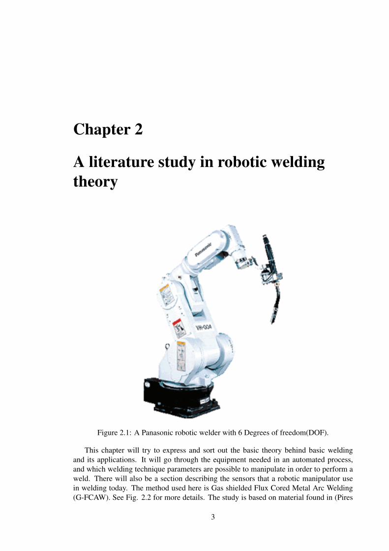
Figure 2.1: A Panasonic robotic welder with 6 Degrees of freedom(DOF).
This chapter will try to express and sort out the basic theory behind basic welding
and its applications. It will go through the equipment needed in an automated process,
and which welding technique parameters are possible to manipulate in order to perform a
weld. There will also be a section describing the sensors that a robotic manipulator use
in welding today. The method used here is Gas shielded Flux Cored Metal Arc Welding
(G-FCAW). See Fig. 2.2 for more details. The study is based on material found in (Pires
3
et al. 2006), (Jiluan 2003), (Grong 1994) and (Nguyen 2004).
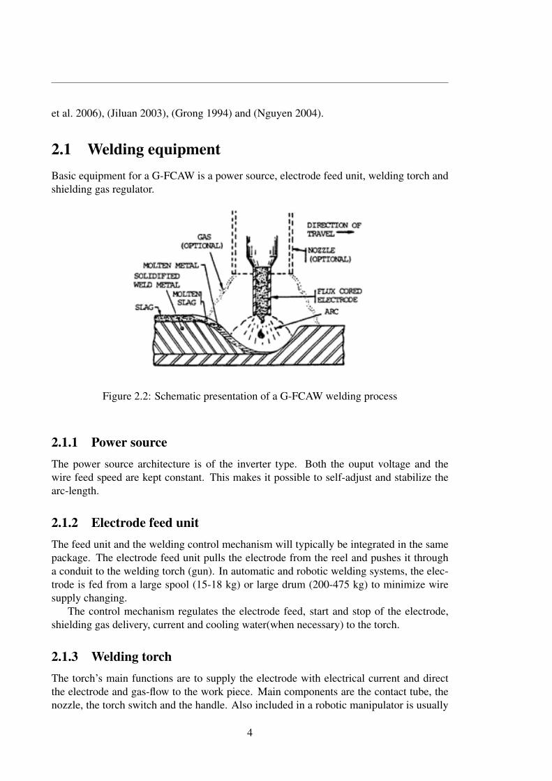
2.1 Welding equipmentBasic equipment for a G-FCAW is a power source, electrode feed unit, welding torch and
shielding gas regulator.
Figure 2.2: Schematic presentation of a G-FCAW welding process
2.1.1 Power sourceThe power source architecture is of the inverter type. Both the ouput voltage and the
wire feed speed are kept constant. This makes it possible to self-adjust and stabilize the
arc-length.
2.1.2 Electrode feed unitThe feed unit and the welding control mechanism will typically be integrated in the same
package. The electrode feed unit pulls the electrode from the reel and pushes it through
a conduit to the welding torch (gun). In automatic and robotic welding systems, the elec-
trode is fed from a large spool (15-18 kg) or large drum (200-475 kg) to minimize wire
supply changing.
The control mechanism regulates the electrode feed, start and stop of the electrode,
shielding gas delivery, current and cooling water(when necessary) to the torch.
2.1.3 Welding torchThe torch’s main functions are to supply the electrode with electrical current and direct
the electrode and gas-flow to the work piece. Main components are the contact tube, the
nozzle, the torch switch and the handle. Also included in a robotic manipulator is usually
4
an emergency-stop mechanism to prevent damage to the robot and the welding torch in the
event of a collision. There is also often included an automatic cleaning mechanism.
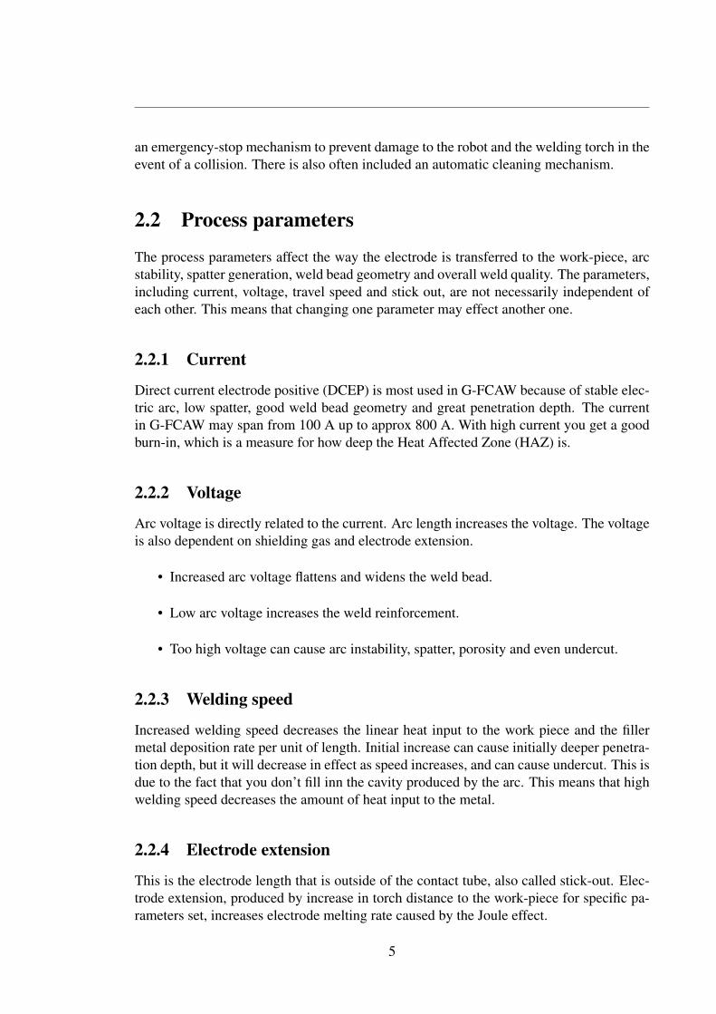
2.2 Process parameters
The process parameters affect the way the electrode is transferred to the work-piece, arc
stability, spatter generation, weld bead geometry and overall weld quality. The parameters,
including current, voltage, travel speed and stick out, are not necessarily independent of
each other. This means that changing one parameter may effect another one.
2.2.1 Current
Direct current electrode positive (DCEP) is most used in G-FCAW because of stable elec-
tric arc, low spatter, good weld bead geometry and great penetration depth. The current
in G-FCAW may span from 100 A up to approx 800 A. With high current you get a good
burn-in, which is a measure for how deep the Heat Affected Zone (HAZ) is.
2.2.2 Voltage
Arc voltage is directly related to the current. Arc length increases the voltage. The voltage
is also dependent on shielding gas and electrode extension.
• Increased arc voltage flattens and widens the weld bead.
• Low arc voltage increases the weld reinforcement.
• Too high voltage can cause arc instability, spatter, porosity and even undercut.
2.2.3 Welding speed
Increased welding speed decreases the linear heat input to the work piece and the filler
metal deposition rate per unit of length. Initial increase can cause initially deeper penetra-
tion depth, but it will decrease in effect as speed increases, and can cause undercut. This is
due to the fact that you don’t fill inn the cavity produced by the arc. This means that high
welding speed decreases the amount of heat input to the metal.
2.2.4 Electrode extension
This is the electrode length that is outside of the contact tube, also called stick-out. Elec-
trode extension, produced by increase in torch distance to the work-piece for specific pa-
rameters set, increases electrode melting rate caused by the Joule effect.
5
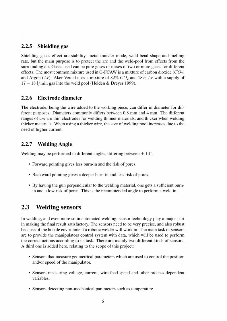
2.2.5 Shielding gas
Shielding gases effect arc-stability, metal transfer mode, weld bead shape and melting
rate, but the main purpose is to protect the arc and the weld-pool from effects from the
surrounding air. Gases used can be pure gases or mixes of two or more gases for different
effects. The most common mixture used in G-FCAW is a mixture of carbon dioxide (CO2)
and Argon (Ar). Aker Verdal uses a mixture of 82% CO2 and 18% Ar with a supply of
17 − 18 l/min gas into the weld pool (Helden & Dreyer 1999).
2.2.6 Electrode diameter
The electrode, being the wire added to the working piece, can differ in diameter for dif-
ferent purposes. Diameters commonly differs between 0.8 mm and 4 mm. The different
ranges of use are thin electrodes for welding thinner materials, and thicker when welding
thicker materials. When using a thicker wire, the size of welding pool increases due to the
need of higher current.
2.2.7 Welding Angle
Welding may be performed in different angles, differing between ± 10◦.
• Forward pointing gives less burn-in and the risk of pores.
• Backward pointing gives a deeper burn-in and less risk of pores.
• By having the gun perpendicular to the welding material, one gets a sufficient burn-
in and a low risk of pores. This is the recommended angle to perform a weld in.
2.3 Welding sensors
In welding, and even more so in automated welding, sensor technology play a major part
in making the final result satisfactory. The sensors need to be very precise, and also robust
because of the hostile environment a robotic welder will work in. The main task of sensors
are to provide the manipulators control system with data, which will be used to perform
the correct actions according to its task. There are mainly two different kinds of sensors.
A third one is added here, relating to the scope of this project:
• Sensors that measure geometrical parameters which are used to control the position
and/or speed of the manipulator.
• Sensors measuring voltage, current, wire feed speed and other process-dependent
variables.
• Sensors detecting non-mechanical parameters such as temperature.
6
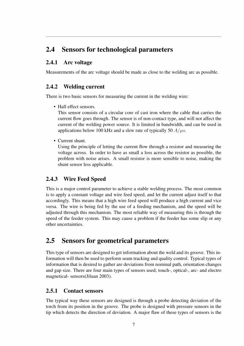
2.4 Sensors for technological parameters
2.4.1 Arc voltageMeasurements of the arc voltage should be made as close to the welding arc as possible.
2.4.2 Welding currentThere is two basic sensors for measuring the current in the welding wire:
• Hall effect sensors.
This sensor consists of a circular core of cast iron where the cable that carries the
current flow goes through. The sensor is of non-contact type, and will not affect the
current of the welding power source. It is limited in bandwidth, and can be used in
applications below 100 kHz and a slew rate of typically 50 A/μs.
• Current shunt.
Using the principle of letting the current flow through a resistor and measuring the
voltage across. In order to have as small a loss across the resistor as possible, the
problem with noise arises. A small resistor is more sensible to noise, making the
shunt sensor less applicable.
2.4.3 Wire Feed SpeedThis is a major control parameter to achieve a stable welding process. The most common
is to apply a constant voltage and wire feed speed, and let the current adjust itself to that
accordingly. This means that a high wire feed speed will produce a high current and vice
versa. The wire is being fed by the use of a feeding mechanism, and the speed will be
adjusted through this mechanism. The most reliable way of measuring this is through the
speed of the feeder system. This may cause a problem if the feeder has some slip or any
other uncertainties.
2.5 Sensors for geometrical parametersThis type of sensors are designed to get information about the weld and its groove. This in-
formation will then be used to perform seam tracking and quality control. Typical types of
information that is desired to gather are deviations from nominal path, orientation changes
and gap size. There are four main types of sensors used; touch-, optical-, arc- and electro
magnetical- sensors(Jiluan 2003).
2.5.1 Contact sensorsThe typical way these sensors are designed is through a probe detecting deviation of the
torch from its position in the groove. The probe is designed with pressure sensors in the
tip which detects the direction of deviation. A major flaw of these types of sensors is the
7
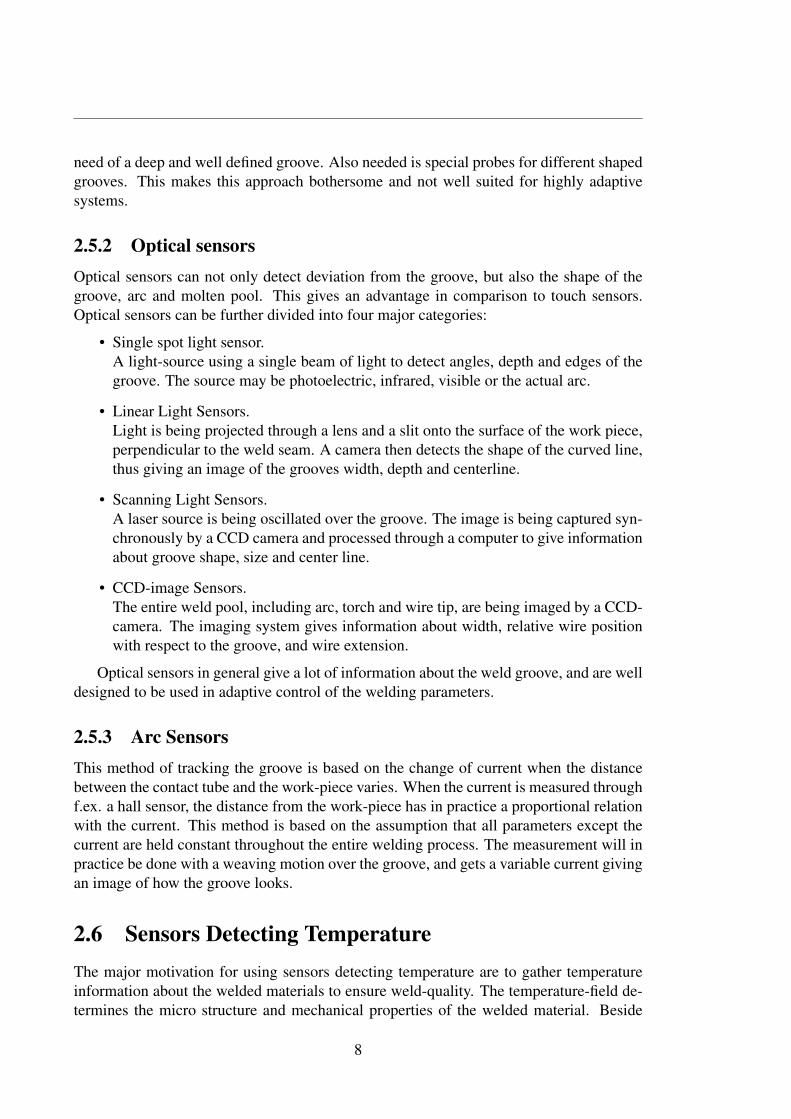
need of a deep and well defined groove. Also needed is special probes for different shaped
grooves. This makes this approach bothersome and not well suited for highly adaptive
systems.
2.5.2 Optical sensorsOptical sensors can not only detect deviation from the groove, but also the shape of the
groove, arc and molten pool. This gives an advantage in comparison to touch sensors.
Optical sensors can be further divided into four major categories:
• Single spot light sensor.
A light-source using a single beam of light to detect angles, depth and edges of the
groove. The source may be photoelectric, infrared, visible or the actual arc.
• Linear Light Sensors.
Light is being projected through a lens and a slit onto the surface of the work piece,
perpendicular to the weld seam. A camera then detects the shape of the curved line,
thus giving an image of the grooves width, depth and centerline.
• Scanning Light Sensors.
A laser source is being oscillated over the groove. The image is being captured syn-
chronously by a CCD camera and processed through a computer to give information
about groove shape, size and center line.
• CCD-image Sensors.
The entire weld pool, including arc, torch and wire tip, are being imaged by a CCD-
camera. The imaging system gives information about width, relative wire position
with respect to the groove, and wire extension.
Optical sensors in general give a lot of information about the weld groove, and are well
designed to be used in adaptive control of the welding parameters.
2.5.3 Arc SensorsThis method of tracking the groove is based on the change of current when the distance
between the contact tube and the work-piece varies. When the current is measured through
f.ex. a hall sensor, the distance from the work-piece has in practice a proportional relation
with the current. This method is based on the assumption that all parameters except the
current are held constant throughout the entire welding process. The measurement will in
practice be done with a weaving motion over the groove, and gets a variable current giving
an image of how the groove looks.
2.6 Sensors Detecting TemperatureThe major motivation for using sensors detecting temperature are to gather temperature
information about the welded materials to ensure weld-quality. The temperature-field de-
termines the micro structure and mechanical properties of the welded material. Beside
8

the fact that mathematical modelling may be used, there exists sensors that measure the
temperature-field with the help from different techniques. There are three main-types of
sensing which are applicable for online use based on infrared radiation:
• Brightness Method.
This method is based on the principle that a body effected by temperature will in-
crease in brightness as temperature increases. As a comparison-reference a standard
calibrated light source is placed next to the object as a means of visual comparison.
• Radiation Method.
This method is based on the principle that the intensity of radiation at a certain wave-
length corresponds to its temperature. Subject to drift, which means that calibration
is important.
• Colorimetric Method.
This method is based on the principle that the ratio of the intensities of two different
radiation wavelengths emitted by a body is a function of its temperature. This gives
the true temperature if it is an ideal black or gray body.
9

Chapter 3
Heat flow modelling
Heat flow modelling is a highly complex and difficult physical phenomena to model. There
has been intense research on this subject for the past decades in order to get better perfor-
mance and quality in welding. This may include the welds ability to withstand mechanical
stress and corrosion. The heat flow equations are governed by partial nonlinear differen-
tial equations. This means that analytical solutions of the equations may be difficult, and
even impossible, to obtain without assumptions, simplifications and loss of generality. The
most important characteristics in welding are the fact that peak temperatures are very high,
temperature gradients are high and temperature fluctuates rapidly. This means that in order
to capture the speed and complexity of the temperature distribution in a welding specimen,
the model needs to have a high order of accuracy. On the other hand, high accuracy often
leads to high order of complexity, which may lead to a model difficult to control. In this
chapter, a mathematical model capturing the wanted characteristics of the problem posed
will be abbreviated.
3.1 The general heat flow equationThe governing equation used here neglects the effects of heat losses due to radiation and
convection as described in (Nguyen 2004). The general equation is
[∂2T
∂x2+∂2T
∂y2+∂2T
∂z2
]=
1
a
∂T
∂t+ f(x, y, z, t), (3.1)
where a is thermal diffusivity of the body material (a = k/ρc), where k is thermal conduc-
tivity, ρ is density and c is specific heat of the material. There are five boundary conditions
to this general case:
1. Prescribed surface temperature: T (x, y, z, t) = f(x, y, z, t).
2. Prescribed heat input: k∂T (x, y, z, t)/∂n = g(x, y, z, t),
where n is normal to the surface.
3. Perfectly insulated surface: ∂T (x, y, z, t)/∂n = 0.
11
4. Convection at the surface: k∂T (x, y, z, t)/∂n = h [T0 − T (x, y, z, t)],
where h is film coefficient of surface conductance.
5. Two-solid bodies in contact: T1(x, y, z, t) = T2(x, y, z, t) and
k1∂T (x, y, z, t)/∂n = k2∂T (x, y, z, t)/∂n
where T1 and T2 are temperatures at the contact surface, and k1 and k2 are the cor-
responding thermal conductivities of the two contact bodies.
In welding, the heat sources may be modelled in such a manner that the effect of radiation
and convection are neglible in comparison to the effect of conduction. This means that
boundary term number 4 and 5 will be neglected in the analysis. This assumption gives
the fact that one regard the welded material as a solid. In reality, the welded metal will go
through phase changes and thus be liquefied for a certain period of time. This is crucial in
real life in order to get a homogeneous material after welding is finished.
3.2 Heat input and arc efficiency factorThe heat-input Q is one of the parameters that effects the temperature the most. This can
be interpreted as the net heat input or energy applied. In general the heat input is defined
as follows:
Q =
(U · I · 60
ν · 1000
)η, (3.2)
where Q is the heat input [kJ/mm], U is the voltage [V ], I is the electric current [A], ν is
the welding speed [mm/min] and η is the arc efficiency factor.
The arc efficiency factor is the factor describing the heat losses due to convection and
radiation. It is defined as follows:
η =q0IU
, (3.3)
where q0 is the net power received by the weldment, and U and I are as described above.
The typical η is in the range of 66 − 85% for G-FCAW.
3.3 The thick plate solutionAs the model in this paper will be made with the help from numerical tools, it is important
to have a comparison reference related to the numerical model. Rosenthal’s Thick Platesolution is used as a reference throughout the modelling. This is because it represents a
good approximation of the posed problem. It is a special result from the general thickplate solution developed by Ryaklin. The deduction of this solution is taken from (Grong
1994). The assumptions made here, are as follows:
The specimen welded on is a semi-infinite body which is isotropic and has an initial tem-
perature T0 limited in one direction by a plane that is impermeable to heat. At initial
time, a point source of constant power q0 moves with constant speed (ν) in the positive
x-direction starting in the origin. The wanted information is the rise of temperature T −T0
in a point P at time t as seen in Fig. (3.1).
12
Over a small time step dt′, the amount of heat released at the surface is dQ = q0dt′.
According to the equation for point source on heavy slab the rise of temperature will be as
follows:
dT =2q0dt
′
ρc [4πa(t− t′)]3/2exp
[− (R′)2
4a(t− t′)
]
=−2q0dt
′′
ρc [4πa(t′′)]3/2exp
[− (R′′)2
4a(t′′)
],
(3.4)
where t′′ = t− t′ is the time available for conduction over the distance
R′ =√
(x0 − νt′)2 + y20 + z2
0 to point P . As this is a representation of the pseudo steady
state solution, the position P must be represented in reference to the moving heat source.
This is done through the shifting of the coordinate system as seen in Fig. (3.1).
y = y0, z = z0, x = x0 + νt
and
x0 + νt′ = x+ νt− νt′ = x+ νt′′.
(3.5)
By inserting this into (3.4) the following expression appears:
dT =−2q0dt
′′
ρc [4πa(t′′)]3/2exp
[− νx
2a)− (R)2
4a(t′′)− ν2t′′
4a
], (3.6)
where R =√x2 + y2 + z2. By substituting the following into (3.6) the total rise of
temperature at P is obtained:
u2 =R2
4at′′, dt′′ = −(
R2
2au3)du
and
m =νR
4a,
m2
u2=ν2t′′
4a.
(3.7)
By integrating between the limits u = R2/4at and u = ∞, this gives the following
integral:
T − T0 =q0
2πλR
(2√π
)exp
(−νx2a
) ∫ ∞
u
exp
(−u2 − m2
u2
)du. (3.8)
The following identity is known:
∫ ∞
0
exp
(−u2 − m2
u2
)du =
√π
2exp
(−νR
2a
).
The general thick plate solution may then be written as:
T − T0 =q0
2πλ
(1
R
)exp
(−νx2a
) [exp
(−νR2a
)− 2√
π
∫ u
0
exp
(−u2 − m2
u2
)du
].
(3.9)
13
The integral will tend to zero when u is sufficiently small. This means that welding has
been performed over a sufficient period of time, giving the pseudo-steady state temperature
distribution known as Rosenthals Thick Plate solution.
T − T0 =q0
2πλ
(1
R
)exp
[− ν
2a(R + x)
]. (3.10)
For further analysis, the equation above is transformed into dimensionless parameters.
According to (Grong 1994), this is done with the following definitions of parameters:
• Dimensionless temperature:
θ =T − T0
Tc − T0
, (3.11)
where Tc is the chosen reference temperature.
• Dimensionless operating parameter:
n3 =q0ν
4πa2ρc (Tc − T0)=
q0ν
4πa2 (Hc −H0)(3.12)
• Dimensionless x-coordinate:
ξ =νx
2a(3.13)
• Dimensionless y-coordinate:
ψ =νy
2a(3.14)
• Dimensionless z-coordinate:
ζ =νz
2a(3.15)
• Dimensionless radius vector:
σ3 =νR
2a(3.16)
• Dimensionless time:
τ =ν2t
2a(3.17)
The dimensionless form of 3.10 is obtained by inserting the above defined parameters:
θ
n3
=
(1
σ3
)exp (−σ3 − ξ) . (3.18)
14
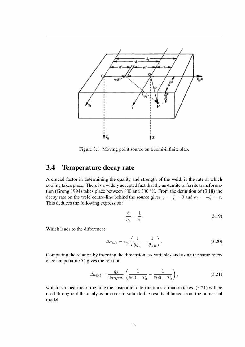
Figure 3.1: Moving point source on a semi-infinite slab.
3.4 Temperature decay rateA crucial factor in determining the quality and strength of the weld, is the rate at which
cooling takes place. There is a widely accepted fact that the austentite to ferrite transforma-
tion (Grong 1994) takes place between 800 and 500 ◦C. From the definition of (3.18) the
decay rate on the weld centre-line behind the source gives ψ = ζ = 0 and σ3 = −ξ = τ .
This deduces the following expression:
θ
n3
=1
τ. (3.19)
Which leads to the difference:
Δτ8/5 = n3
(1
θ500
− 1
θ800
). (3.20)
Computing the relation by inserting the dimensionless variables and using the same refer-
ence temperature Tc gives the relation
Δt8/5 =q0
2πaρcν
(1
500 − T0
− 1
800 − T0
), (3.21)
which is a measure of the time the austentite to ferrite transformation takes. (3.21) will be
used throughout the analysis in order to validate the results obtained from the numerical
model.
15
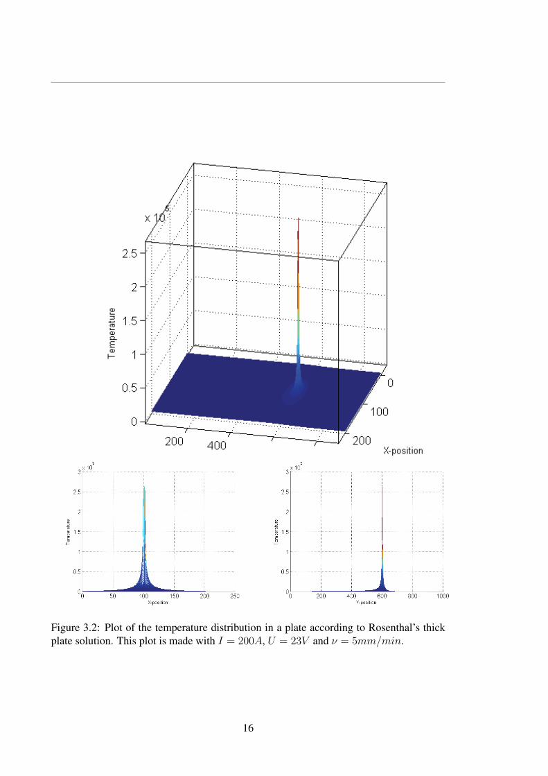
Figure 3.2: Plot of the temperature distribution in a plate according to Rosenthal’s thick
plate solution. This plot is made with I = 200A, U = 23V and ν = 5mm/min.
16
Chapter 4
The finite element method
Modelling of physical phenomena may be done in several ways. For a long time, the
governing method of analysis has been the analytical one, where a mathematical model is
derived from the governing set of equations. This is a very powerful method of analysis,
but has its drawback in the way it handles large problems with advanced dynamics. In
recent decades the increase in computer power has changed this to a large extent. It is
now possible to simulate and solve large sets of equations through numerical modelling.
There has been developed many ways of modelling in the numerical manner. One of the
most used, and certainly one of the most powerful ones, is the Finite Element Method
(FEM). On the FEM one may apply partial differential equations (PDE’s) on complicated
geometries with boundary conditions. This makes it immensely versatile and flexible.
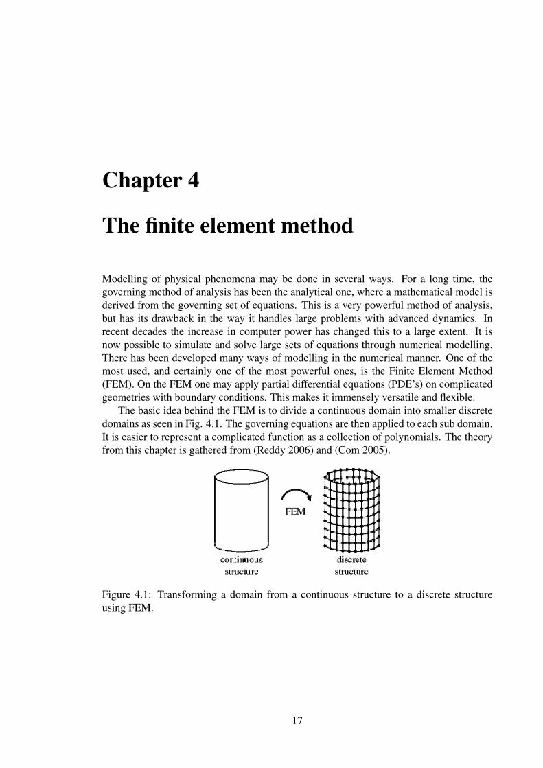
The basic idea behind the FEM is to divide a continuous domain into smaller discrete
domains as seen in Fig. 4.1. The governing equations are then applied to each sub domain.
It is easier to represent a complicated function as a collection of polynomials. The theory
from this chapter is gathered from (Reddy 2006) and (Com 2005).
Figure 4.1: Transforming a domain from a continuous structure to a discrete structure
using FEM.
17
4.1 The basic features of the methodThe method is characterized by three basic features which makes it superior to other nu-
merical methods:
• A geometrical domain is represented as a collection of smaller sub domains with
simple geometrical shape called finite elements, as seen in Fig. 4.1. Each element is
seen as an independent domain by itself.
• The governing equations of the problem are applied to develop algebraic expressions
over each single sub domain.
• The independent domains are, with a governing equation, put back together to their
respective position using certain inter element relationships.
The whole method includes three stages, and they are all based on numerical modelling,
and will thus be an approximation of the real physical phenomena. This introduce errors in
all the three stages of the modelling. In the sub domain division into finite elements there
may be elements which make the assembled sub domains not fitting the original domain.
The unknowns u in the element-equation derivation are approximations using the basic
idea that a continuous function can be a linear combination of known functions φi and
undetermined coefficients ci, making u ≈ ∑ciφi. The relation between the unknowns
ci are determined satisfying the governing equations in a weighted integral sense. φi are
polynomials often determined through interpolation theory. This introduces errors both in
representing u and evaluating the integrals. Last of all, errors are introduced in solving the
assembled system of equations.
Some of the above discussed errors may be zero. If all errors are zero, the solution
is exact. This is in most cases not the fact. The magnitude of the errors will decrease as
the resolution of the grid introduced increases. Through the rise in computer-power, the
possibility of increased accuracy has risen immensely the last couple of decades. For more
thorough explanations on the basic theory behind the FEM, look in chapter 1 of (Reddy
2006).
4.2 The weighted integral and weak form formulationsIn classical terms the variational principle is a way of creating a set of equations equivalent
to the governing equations of the problem. The modern way of defining the variational
principle is to transform the governing equations into weighted integral-statements. The
weighted integral may be used to express almost all physical principles.
4.2.1 The weighted integral statementThe solution of differential and/or integral equations is almost always, when using approx-
imate methods, in the form:
u(x) ≈ UN(x) =N∑
j=1
cjφj(x), (4.1)
18
where u represents the exact solution of the particular equation and associated boundary
conditions, and UN is its approximation. The approximate UN is represented as a linear
combination of unknown parameters cj and known functions φj of position x on domain
Ω, where the problem is posed. To obtain the approximate solution, one needs to find
N algebraic relations among the N parameters c1, c2, ... , cN . The sum of all these
coefficients give the approximate solution of UN . If one can find a UN that satisfies the
governing differential equation in every point x on the domain Ω, and satisfying boundary
conditions, then the solution is exact.
When trying to find an exact solution on the form of (4.1), working from known poly-
nomials φj , the exact solution satisfying the boundary conditions may give no solution to
the equations because of inconsistence in the statement of the equations. In order to bypass
this problem, the weighted integral has some preferable features.∫ 1
0
w(x)Rdx = 0, (4.2)
where w(x) is called a weight function and R denotes the differential equation called the
residual. This is defined as,
R ≡ −dUN
dx− x
d2UN
dx2+ UN .
From (4.2), we obtain as many linearly independent equations as there are linearly inde-
pendent functions of w(x).The advantage is that with the integral (4.2) stated as it is, one gets all higher order
terms cancelled out because of the limits set, and does not get inconsistency in determining
the unknown coefficients as one gets in the original case. In addition, the number of
choices of w must be restricted to N , so that there is the same number of equations as
there are unknown coefficients cj . For more info look in chapter 2.1. of (Reddy 2006).
4.2.2 The weak formAs the FEM is a method of determining approximate solutions of larger systems, the
boundary conditions of the problem are also crucial to be fulfilled. The weak form facil-
itates these problems in an elegant way. It classifies the boundary conditions into natural
and essential types. It is defined to be a weighted-integral statement of a differential equa-
tion in which the differentiation is transferred from the dependent variable to the weight
function such that all natural boundary conditions of the problem are included in the inte-
gral statement.
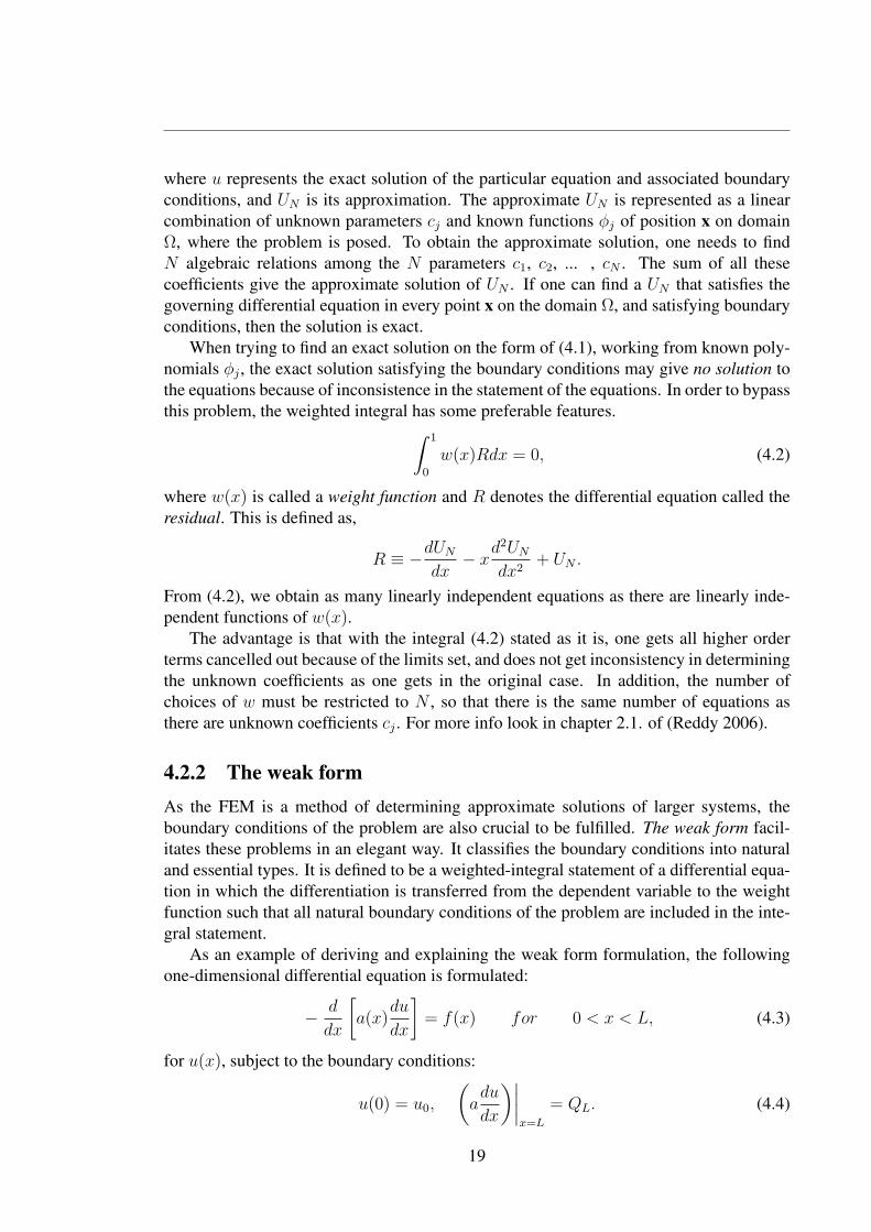
As an example of deriving and explaining the weak form formulation, the following
one-dimensional differential equation is formulated:
− d
dx
[a(x)
du
dx
]= f(x) for 0 < x < L, (4.3)
for u(x), subject to the boundary conditions:
u(0) = u0,
(adu
dx
)∣∣∣∣x=L
= QL. (4.4)
19
Here a(x) and f(x) are known functions of x, and u0 and QL are known values. L is
the size of the one-dimensional domain. The boundary conditions are said to be non-
homogeneous when the specified values are nonzero, and homogeneous when they are
zero.
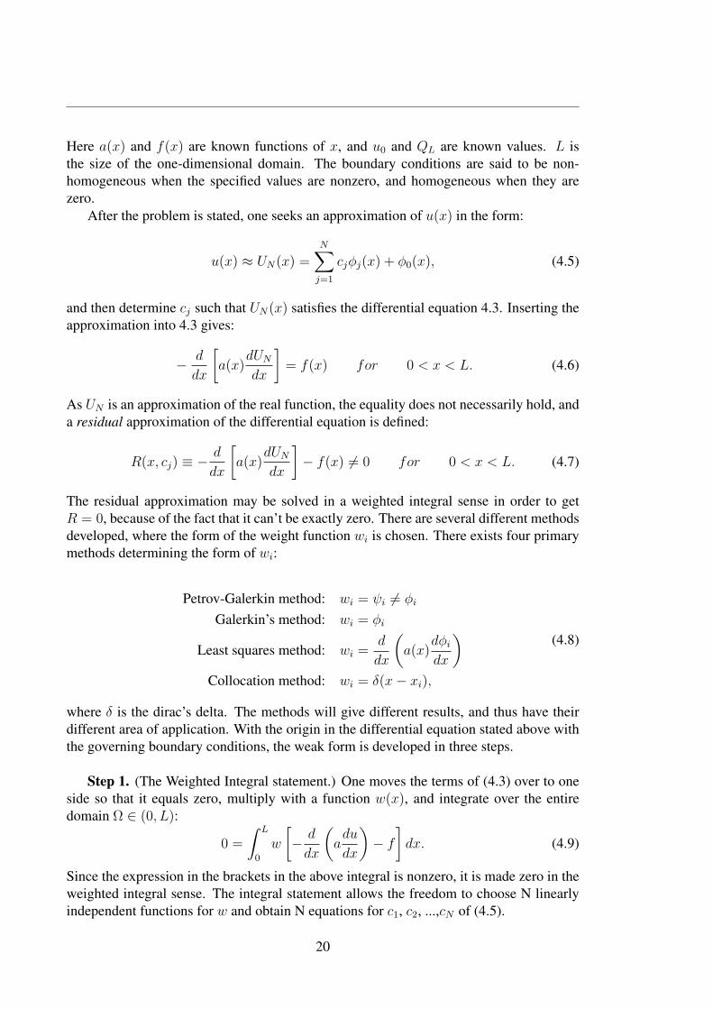
After the problem is stated, one seeks an approximation of u(x) in the form:
u(x) ≈ UN(x) =N∑
j=1
cjφj(x) + φ0(x), (4.5)
and then determine cj such that UN(x) satisfies the differential equation 4.3. Inserting the
approximation into 4.3 gives:
− d
dx
[a(x)
dUN
dx
]= f(x) for 0 < x < L. (4.6)
As UN is an approximation of the real function, the equality does not necessarily hold, and
a residual approximation of the differential equation is defined:
R(x, cj) ≡ − d
dx
[a(x)
dUN
dx
]− f(x) �= 0 for 0 < x < L. (4.7)
The residual approximation may be solved in a weighted integral sense in order to get
R = 0, because of the fact that it can’t be exactly zero. There are several different methods
developed, where the form of the weight function wi is chosen. There exists four primary
methods determining the form of wi:
Petrov-Galerkin method: wi = ψi �= φi
Galerkin’s method: wi = φi
Least squares method: wi =d
dx
(a(x)
dφi
dx
)
Collocation method: wi = δ(x− xi),
(4.8)
where δ is the dirac’s delta. The methods will give different results, and thus have their
different area of application. With the origin in the differential equation stated above with
the governing boundary conditions, the weak form is developed in three steps.
Step 1. (The Weighted Integral statement.) One moves the terms of (4.3) over to one
side so that it equals zero, multiply with a function w(x), and integrate over the entire
domain Ω ∈ (0, L):
0 =
∫ L
0
w
[− d
dx
(adu
dx
)− f
]dx. (4.9)
Since the expression in the brackets in the above integral is nonzero, it is made zero in the
weighted integral sense. The integral statement allows the freedom to choose N linearly
independent functions for w and obtain N equations for c1, c2, ...,cN of (4.5).
20

At this point the boundary conditions of the problem is not included. Since the weight-
function can be any non-zero integrable function, and has no differentiability requirements,
it may be exploited.
Step 2.When developing the weak term, one makes some changes in comparison to
when solving the conventional weighted integral. The weighted integral statement de-
mands that UN (see (4.5)) is differentiable as many times as called for in the original
differential equation(see (4.3)), and satisfy the specified boundary conditions.
When the approximate functions φj are such that UN is not continuously differentiable,
as in many cases, one makes use of φj for w ∼ wi. It will then make sense to shift half of
the derivatives from u to w so that both are equally differentiated, and thus there will be
fewer or weaker continuity requirements on φj . This is known as the weak formulation,
and has two desirable characteristics. The dependent variable requires a weaker continuity,
and always result in a symmetric coefficient matrix for self-adjoint equations. The other
characteristic is that the natural boundary conditions are included in the weak form, and
UN is only required to satisfy the essential boundary conditions of the problem.
The primary variable of the problem in this case is the dependent variable u expressed
in the same form as the weight function (w) appearing at the boundary. By performing the
integral of (4.9), and introducing the variables, the equation becomes:
Q ≡(adu
dx
)nx, (4.10)
Q represents the heat, and is called a secondary variable, nx is the direction cosine, which
is simply the angle between positive x-axis and the normal to the boundary. We then get
the following result:
0 =
∫ L
0
(adw
dx
du
dx− wf
)dx−
[wa
du
dx
]L
0
=
∫ L
0
(adw
dx
du
dx− wf
)dx− (wQ)0 − (wQ)L,
(4.11)
and nx = ±1 respectively. (4.11) is called the weak form of (4.3). The reason for the term
weak is its reduced demand for continuity of u. In (4.9) u had to be twice differentiable,
as in (4.11) it is only demanded once differentiable.
Step 3. The last step of the weak formulation is to impose the actual boundary condi-
tions under consideration. One demands that the weight function w vanish at the specific
boundary points. In other words, w has to satisfy the homogeneous form of the specified
essential boundary conditions. To clarify, look at the above defined problem with bound-
ary conditions (4.4). The essential boundary condition is u = u0 and (adu/dx)|x=L = QL
is the natural condition. Then (4.11) reduces to:
0 =
∫ L
0
(adw
dx
du
dx− wf
)dx− w(L)QL, (4.12)
21

because the weight function w(0) = 0, and
Q(L) =
(adu
dxnx
)∣∣∣∣x=L
=
(adu
dx
)∣∣∣∣x=L
= QL. (4.13)
(4.12) is the weak form equivalent to the original (4.3) and natural boundary condition
(4.4).
4.2.3 SummaryTo summarize, the weak form of a differential equation is a weighted integral statement
which is the equivalent to the differential equation and its specified natural boundary con-
ditions. It is possible to specify a weak form for all differential equation problems, linear
or non-linear. There are three basic steps in the development of the weak form. All expres-
sions are set equal to zero, then the entire equation is multiplied with a weight function w.
The resultant statement is then integrated over the entire domain, and the resulting state-
ment is called the weighted-integral form. One then integrate by parts in order to distribute
the differentiations between the dependent variable and the weight-function. The bound-
ary terms are used to identify the form of the primary and secondary variables. At last, the
boundary terms are modified by restricting the weight function to satisfy the homogeneous
form of the specified essential boundary conditions and replacing the secondary variables
by their specified values.
The whole purpose of the weak form and/or the weighted integral statement is to obtain
as many algebraic equations as there are unknowns in the approximation of the dependent
variables of the equation.
22
Chapter 5
Model order reduction
When modelling phenomena which have a complex nature, the order of the equations de-
scribing the problem may reach very high order of complexities. This results in many
states in the state-space making it infeasible to use in controller design. In order to bypass
this problem, model order reduction is a powerful tool, which goal is to systematically
develop a low-order model that catches the relevant system dynamics over an adequate
range of frequencies and forcing inputs. There exists many different techniques for reduc-
ing the order of the model. They all have different advantages and prerequisites. Common
for most of them, is that the resulting reduced model does not represent anything physical
anymore. The states can not be associated with the physics in the original model. It may
be seen as a black box, where the inputs and outputs of the model are the only known
parameters related to the original physics. In this project, the model is linear but has a
very large number of states. With this in mind, many of the methods existing will not be
investigated, and throughout this chapter the emphasis will be put on the following four
methods:
• Proper Orthogonal Decomposition(POD)
• Rational Krylov algorithms
• Fourier model reduction
• Balanced realization and truncation
POD will be used as the reduction technique in the consecutive work, whereas the three
last methods mentioned are meant as an introductionary study. The chapter is a literature
study on model order reduction, and the methods described here are found in the following
articles: (Willcox & Megretski 2005), (Gugercin et al. 2004), (Olsson 2002), (Gugercin
& Wilcox 2007), (Hovland & Gravdahl 2006), (Camp & King 1997), (Astrid 2004) and
(Cazemier 1997)
23
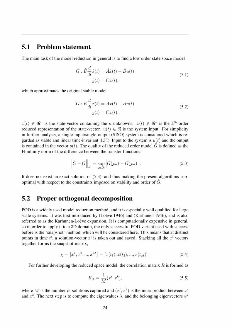
5.1 Problem statementThe main task of the model reduction in general is to find a low order state space model
G : Ed
dtx(t) = Ax(t) + Bu(t)
y(t) = Cx(t),(5.1)
which approximates the original stable model
G : Ed
dtx(t) = Ax(t) +Bu(t)
y(t) = Cx(t).(5.2)
x(t) ∈ n is the state-vector containing the n unknowns. x(t) ∈ k is the kth-order
reduced representation of the state-vector. u(t) ∈ is the system input. For simplicity
in further analysis, a single-input/single-output (SISO) system is considered which is re-
garded as stable and linear time-invariant (LTI). Input to the system is u(t) and the output
is contained in the vector y(t). The quality of the reduced order model G is defined as the
H-infinity norm of the difference between the transfer functions:
∥∥∥G−G∥∥∥∞
= supω∈�
∣∣∣G(jω) −G(jω)∣∣∣ . (5.3)
It does not exist an exact solution of (5.3), and thus making the present algorithms sub-
optimal with respect to the constraints imposed on stability and order of G.
5.2 Proper orthogonal decompositionPOD is a widely used model reduction method, and it is especially well qualified for large
scale systems. It was first introduced by (Loève 1946) and (Karhunen 1946), and is also
referred to as the Karhunen-Loève expansion. It is computationally expensive in general,
so in order to apply it to a 3D domain, the only successful POD variant used with success
before is the "snapshot" method, which will be considered here. This means that at distinct
points in time ti, a solution-vector xi is taken out and saved. Stacking all the xi vectors
together forms the snapshot-matrix,
χ =[x1, x2, ..., xM
]= [x(t1), x(t2), ..., x(tM)] . (5.4)
For further developing the reduced space model, the correlation matrix R is formed as
Rik =1
M(xi, xk), (5.5)
where M is the number of solutions captured and (xi, xk) is the inner product between xi
and xk. The next step is to compute the eigenvalues λi and the belonging eigenvectors ψi
24

of R. These are used to form the POD basis vectors, and are given as a linear combination
of snapshots. The jth POD basis vector, Φj , is given as
Φj =M∑i=1
ψjix
i, (5.6)
where ψji denotes the ith element of the jth eigenvector. The magnitude of the eigenvalues
describes the relative importance of the corresponding POD-basis vector. Identifying and
choosing a sufficient amount of basis-vectorsN , mirroring the sufficient amount of energy
from the snapshot matrix, gives the total projection-matrix Φ =∑N
j=1 Φj . The reduced
space matrices described in (5.1) are obtained as follows,
E = ΦTEΦ ∈ k×k,
A = ΦTAΦ ∈ k×k,
B = ΦTB ∈ k×1,
C = CΦ ∈ 1×k.
(5.7)
When the computation of the orthonormal set of POD vectors is done, the reduced order
model is obtained by projecting the solution of the original system onto the reduced-space
basis
x(t) =M∑i=1
xi(t)Φi. (5.8)
Substituting this into (5.2) and using orthogonality, the reduced order system (5.1) is ob-
tained. Normally the snapshots are taken from simulations of the original system. A
problem is that the reduced order model will only mirror dynamics from the snapshots
taken. This means that inputs to the simulations has to be chosen with great care. This
may lead to problems in many applications. Snapshots may not always be accessible di-
rectly from a process. This may have several reasons. It is possible to bypass this problem
by applying the POD in the frequency domain, but the frequency domain approach has an
extensive computational cost and will not be regarded here. Other characteristics of POD,
is that it does not guarantee the quality and stability of reduced order models, even though
the original system itself is stable. This gives rise to the need for tuning in applications
reduced with POD. POD is not an exact science. The heuristic criterion
P =
∑ki=1 σ
2i∑M
i=1 σ2i
, (5.9)
may be used as an indication of the amount of energy conserved in the model reduced
order model. The number of basis functions k denotes the number of states in the reduced
order model. If P ≈ 1, then almost all the energy is captured in the system.
5.3 Rational Krylov algorithmsWhen working with Krylov based methods, one takes origin in the systems transfer func-
tion
G(s) = C(sI − A)−1B. (5.10)
25
The reduced order transfer function G(s) is obtained through interpolation with G(s) and
some of its derivatives (called moments) at some points σk in the complex plane. Mathe-
matically speaking, this means that one wants to find the matrices A, B and C so that
(−1)j
j!
djG(s)
dsj
∣∣∣∣s=σk
= C(σkI−A)−(j+1)B = C(σkI−A)−(j+1)B =(−1)j
j!
djG(s)
dsj
∣∣∣∣∣s=σk
,
(5.11)
where k = 1, ..., K and j = 1, ..., J . K is the number of interpolation points σk and J is
the number of moments to be matched at each interpolation point. When interpolating, it
is desired to match the moments at several frequencies spanning the operation-frequency
range of the system. This is done due to the fact that if one only matches the moment at one
frequency, it will often lead to a very large error at other frequencies. However, it is very
expensive to compute each single interpolation-point explicitly, and the rational Krylov
method amongst others, is capable of computing G(s) without computing them explicitly.
This is very important because of the fact that it is a very time-consuming operation to
perform, and thus one of the main motivations behind the rational Krylov based methods.
A Krylov space is defined as
Kj(F, g;σ) := Im([g Fg F 2g ... F j−1g
])if σ = ∞,
Kj(F, g;σ) := Im([
(σI − F )−1g ... (σI − F )−jg])
if σ �= ∞,(5.12)
where matrix F ∈ n×n, vector g ∈ n and point σ ∈ are the constructs of the Krylov
space defined for index j.When creating the reduced Krylov space, one needs to create the following two matri-
ces:
Range(V ) = Span [Kj1(A,B;σ1), ..., KjK(A,B;σK)]
Range(Z) = Span[KjK+1
(AT , CT ;σK+1), ..., Kj2K(A,B;σ2K)
],
(5.13)
which then gives the property ZTV = I . This gives the reduced order model G(s) =CV (sI − ZTAV )−1ZTB matching jk number of moments of G(s) at each consecutive
interpolation point σk. So to construct the reduced order model, all one has to do is to
construct matrices V and Z as described above. This makes the method computationally
efficient because it can be implemented iteratively due to the fact that one only require
some matrix-vector multiplications and some sparse linear solvers.
5.4 Fourier model reductionThis method for performing model reduction is similar to that of Krylov, but is is done in
the discrete frequency domain. This means that one needs to put the transfer function over
into discrete form. This is done by inserting the identity
z =s+ ω0
s− ω0
, (5.14)
into
G(s) = g(z) = c(zI − a)−1b, (5.15)
26
and
d = C(ω0I − A)−1B,
a = −(ω0I + A)(ω0I − A)−1,
c = 2ω0C(ω0I − A)−1,
b = −I(ω0I − A)−1B,
(5.16)
and ω0 is some fixed positive real number. To complete the discrete time transform ofG(s)the following fourier decomposition is used
G(s) =∞∑
j=0
Gj
(s− ω0
s+ ω0
)j
, (5.17)
where
G0 = d, Gj = caj−1b (j = 1, 2...). (5.18)
The fourier expansion just performed converges exponentially for |z| > ρ(a) where ρ(a)denotes the spectral radius of a, which is the maximal absolute value of a’s eigenvalues.
The first m coefficients are calculated using the computationally cheap iterative process
Gj = chj−1, hj = ahj−1(j = 1, ...,m), (5.19)
where h0 = b. It is expected to be stable because ρ(a) < 1.
For further development, the m + 1 fourier coefficients are used to construct a mth
order state-space model
g : x[t+ 1] = ax[t] + bu[t], y[t] = cx[t], (5.20)
where
a =
⎡⎢⎢⎢⎢⎢⎣
0 0 0 0 ...1 0 0 0 ...0 1 0 0 ...0 0 1 0 ...
0 0 0. . .
⎤⎥⎥⎥⎥⎥⎦, b =
⎡⎢⎢⎢⎣
100...
⎤⎥⎥⎥⎦ , c =
[g1 g2 . . . gm
], (5.21)
consists of up to several hundred states. It is possible to further reduce this by applying
balanced truncation, which will be described in the next section. For use in balanced
truncation, the controllability matrix is the identity matrix and the observability matrix is
the Hankel matrix with c as the first row. By computing the singular vectors from the mth
order Hankel matrix
Γ =
⎡⎢⎢⎢⎢⎢⎢⎢⎣
g1 g2 g3 . . . gm−1 gm
g2 g3 g4 . . . gm 0g3 g4 g5 . . . 0 0...
......
......
gm−1 gm 0 . . . 0 0gm 0 0 . . . 0 0
⎤⎥⎥⎥⎥⎥⎥⎥⎦, (5.22)
27
the balancing vectors can be obtained. The Hankel singular values are given by the singular
values of Γ and is denoted as σi, i = 1, 2, . . . ,m. Finally, the low-order model can be
obtained using the following relationships
A = ω0(a− I)−1(a+ I), (5.23)
B = 2ω0(a− I)−1b, (5.24)
C = −c(a− I)−1, (5.25)
(5.26)
which completes the reduction through fourier techniques.
5.5 Balanced realization and truncationThe procedure called balanced truncation is a method based on finding and eliminating
states that are difficult to control or to observe in the state space realization (5.2) and
obtaining the reduced order model (5.1). The procedure is time-consuming and will not be
applicable for very large scale systems due to need of large amounts of computer power.
To identify controllable and observable states, the controllability grammian
LB =
∫ ∞
0
eAtBBT eAT tdt, (5.27)
and the observability grammian
LC =
∫ ∞
0
eAT tCCT eAtdt, (5.28)
are defined. The reachable states are denoted by LC and the observable ones by LB.
Both grammians are realization dependent, meaning that two different state-space systems
which give the same transfer function, may have different grammians. A realization may
have few controllable states but many observable states and vice versa. This problem is
called balanced realization. Here states that are difficult to control coincide with states that
are difficult to observe, and are realized as
LB = LC = diag(σ1, σ2, . . . , σn, . . .), σ1 ≥ σ2 ≥, . . . ,≥ 0, (5.29)
where σi =√λi(LBLC) are the Hankel singular values and realization invariant. The
balancing transformation T can be found from the following algorithm:
• Compute LB and LC from (5.2) which will be defined as∑
in the following.
• Following the fact that LB is symmetric and positive definite, the Cholesky decom-
position gives LB = RTR.
• Compute RTLCR = U∑
2UT where∑
2 = diag(σi)∞i=1 and U is unitary.
• Defining T =∑ 1
2UTR, where it follows that (T−1)TLCT−1 =
∑= TLBT
T .
T then gives rise to the balanced state space realization denoted as∑(Abal, Bbal, Cbal) =
∑(TAT−1, TB,CT−1). (5.30)
This concludes the balanced realization and truncation technique.
28
Chapter 6
Numerical modelling and analysis ofheat flow in a single-pass butt weldingseam
The problem investigated here, and as earlier described, is to model the heat-flow in a
robotic weld. There are some assumptions made when studying the problem, which are
regarded as reasonable. The whole process of multi pass-welding is very complex. From
the fact that experience shows that the last pass of a weld is the most critical one (Grong
1994), the last pass of the weld will be the one analyzed here. The heat source is regarded
as an optimal point source, moving at constant speed. The reason for this is to make
the model as closely related as possible to the analytical solution used as a reference. The
numerical modelling is done in a GUI-based program called Comsol MultiphysicsTM. The
program is based on the theory explained in Chapter (4) about the FEM. The mass added
in a pass of a weld is neglected, and the model simply becomes the equivalent to that of a
Tungsten Inert Gas (TIG) source moving across the plate without adding filler-wire.
6.1 Construction of the model
The first approach to describe the problem using a mathematical model, was to create a
single-pass weld in a 50mm thick plate. The heat source passed once over the plate on the
top surface. The results, were as earlier described, compared to the solution deduced by
Rosenthal.
As shown in Fig.(6.1), the mesh is refined along the centre line of the plate. This is
where the heat-source is moved across, and this is done for two reasons. One reason is
to make the model with as low complexity as possible, and to make the solution more
exact along the line where the heat source is moved. The model itself is made with the
same assumptions as the analytic solution. This means that the source is a point source,
moved with a constant speed along the center line. The model itself takes into account
transient effects. When comparing with the analytical solution, snapshots are taken of
the temperature as a function of the position, as seen in Fig. (6.2). For more detailed
information on how the model was made, see in Appendix A.
29
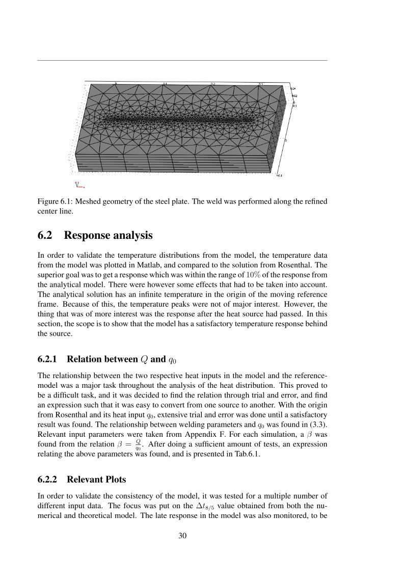
Figure 6.1: Meshed geometry of the steel plate. The weld was performed along the refined
center line.
6.2 Response analysisIn order to validate the temperature distributions from the model, the temperature data
from the model was plotted in Matlab, and compared to the solution from Rosenthal. The
superior goal was to get a response which was within the range of 10% of the response from
the analytical model. There were however some effects that had to be taken into account.
The analytical solution has an infinite temperature in the origin of the moving reference
frame. Because of this, the temperature peaks were not of major interest. However, the
thing that was of more interest was the response after the heat source had passed. In this
section, the scope is to show that the model has a satisfactory temperature response behind
the source.
6.2.1 Relation between Q and q0The relationship between the two respective heat inputs in the model and the reference-
model was a major task throughout the analysis of the heat distribution. This proved to
be a difficult task, and it was decided to find the relation through trial and error, and find
an expression such that it was easy to convert from one source to another. With the origin
from Rosenthal and its heat input q0, extensive trial and error was done until a satisfactory
result was found. The relationship between welding parameters and q0 was found in (3.3).
Relevant input parameters were taken from Appendix F. For each simulation, a β was
found from the relation β = Qq0
. After doing a sufficient amount of tests, an expression
relating the above parameters was found, and is presented in Tab.6.1.
6.2.2 Relevant Plots
In order to validate the consistency of the model, it was tested for a multiple number of
different input data. The focus was put on the Δt8/5 value obtained from both the nu-
merical and theoretical model. The late response in the model was also monitored, to be
30
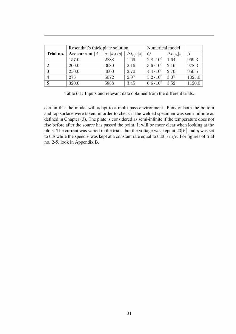
Rosenthal’s thick plate solution Numerical model
Trial no. Arc current [A] q0 [kJ/s] Δt8/5[s] Q Δt8/5[s] β1 157.0 2888 1.69 2.8 · 106 1.64 969.32 200.0 3680 2.16 3.6 · 106 2.16 978.33 250.0 4600 2.70 4.4 · 106 2.70 956.54 275 5072 2.97 5.2 · 106 3.07 1025.05 320.0 5888 3.45 6.6 · 106 3.52 1120.0
Table 6.1: Inputs and relevant data obtained from the different trials.
certain that the model will adapt to a multi pass environment. Plots of both the bottom
and top surface were taken, in order to check if the welded specimen was semi-infinite as
defined in Chapter (3). The plate is considered as semi-infinite if the temperature does not
rise before after the source has passed the point. It will be more clear when looking at the
plots. The current was varied in the trials, but the voltage was kept at 23[V ] and η was set
to 0.8 while the speed ν was kept at a constant rate equal to 0.005 m/s. For figures of trial
no. 2-5, look in Appendix B.
31
6.3 Discussion
The results obtained in this chapter are based on numerical modelling done by the FEM,
and will never be an exact copy of real life. This is however not the objective of the
modelling. As this model in future work will be used in a control context, one would
like a model which is reasonable in its physics, and still be as simple as possible. Errors
in the modelling will be taken care of by the closed loop system. Because of this, one
can allow simplifications and errors. In this model, the target was to stay within 10% of
the reference temperature when looking at the temperature response before and after the
heat-source has passed. The response in front of the heat-source comes from the physical
fact that heat conducts forward in the material, and the slopes abruptness will follow from
the heat-input and the welding speed. A high speed will thus give a steep curve, while a
high heat-input will slacken the gradient. In the tests performed in this work, the speed
has been kept constant and the only parameter which has been changed is the current. This
is a valid assumption due to the fact that speed is kept constant in most robotic welding
applications, and the only parameter being changed is the current and voltage.
The response in front of the heat-source is not of great importance, but is a good
indicator for the validity of the model. The results show that the temperature in both
model and reference starts to rise at the same point on the plate. The reference will, due
to the singularity in origin rise to infinity, and thus have a gradient ∇T → ∞. For the
model, this will lead to significant deviance close to the origin. When looking in Fig.6.2c
and Appendix B, it may be observed that the curves of the model shows some signs of
low resolution. This is simply due to the fact that the curve from the FEM-model only is
sampled each 0.5 second.
The peak temperature is not much emphasized in this projects work. The reference
model has a singularity in the origin, and will in that point give an infinite temperature.
The model will also not be completely valid at peak temperatures, because of the resolution
of the mesh along the center line.
The response after the source has passed is more or less an equivalent to the heat
equation in the homogeneous form, and is governed by the initial temperature and the
physical properties of the material. The rate at which the temperature decays, will be
reasonably low, meaning that the model will be able to follow with greater accuracy. This
also means that the relatively coarse resolution of the mesh will be of less importance
when reaching the point at which the temperature is in the transition between 800◦C and
500 ◦C. This transition period is the one with highest priority. As earlier described, this is
the interval at which the austentite to ferrite transformation takes place, and the mechanical
properties of the weld is established. To secure this characteristic, it is important to keep
Δt8/5 as close to constant as possible for the whole length of the bead. It can be seen from
the plots of the temperature response in Fig.6.2 and Appendix B, with the relation on βestablished, that the two trajectories are close to each other.
One of the criteria for the model of Rosenthal to be valid, is that the welded specimen
is semi-infinite, as explained earlier. Looking at Fig.6.3, it can be seen that the plate
experiences complete penetration at each pass. This will not make the model valid for this
case. The present would be valid for a medium-thick plate solution, but as this is not part
of the scope of this project, it will not be further pursued. A remedy for this is to simply
32
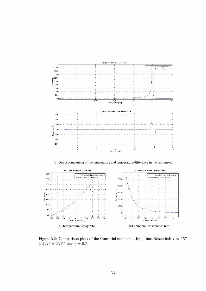
(a) Direct comparison of the temperature and temperature-difference in the responses.
(b) Temperature decay rate. (c) Temperature increase rate
Figure 6.2: Comparison plots of the from trial number 1. Input into Rosenthal: I = 157[A] , U = 23 [V ] and η = 0.8.
33

Figure 6.3: Temperature plot of the bottom surface of the welded plates. The different
curves represents the different inputs into the model.
increase the plate thickness in the numerical model. Due to limitations in computer-power
when performing the simulations, it was not possible to increase plate thickness in the
present case. An increase in plate-thickness would make the model more closely related
to the reference model, and thus giving a better response.
From Fig.6.6 and Table 6.1, one may analyze the data acquired and see how well the
model performs. If one starts to look at Fig.6.6a, which is a presentation of the different
Δt8/5 found from the trials, it can be seen that the two values found for each consecutive
test are close to each other. As expected the cooling time increases with heat-input. It can
be seen from Fig.6.2 and Appendix B, that the shape of the curves are completely decou-
pled from the input. The interval Δt8/5 will occur at a later position in the temperature
response, and thus have a slacker gradient giving a longer cooling time in the specified in-
terval. Fig.6.6c shows the plots of the percentage deviation the numerical model has from
the two different references. It can be seen that all trials are well within 10% of the ana-
lytic solution with the maximal deviation of 3.22%. Which is a good result, regarding the
problem with not being able to make a model satisfying the semi-infinte body requirement.
34
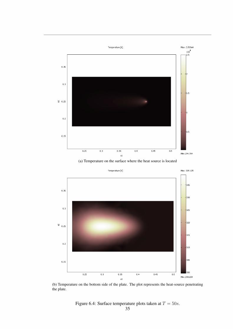
(a) Temperature on the surface where the heat source is located
(b) Temperature on the bottom side of the plate. The plot represents the heat-source penetrating
the plate.
Figure 6.4: Surface temperature plots taken at T = 50s.35
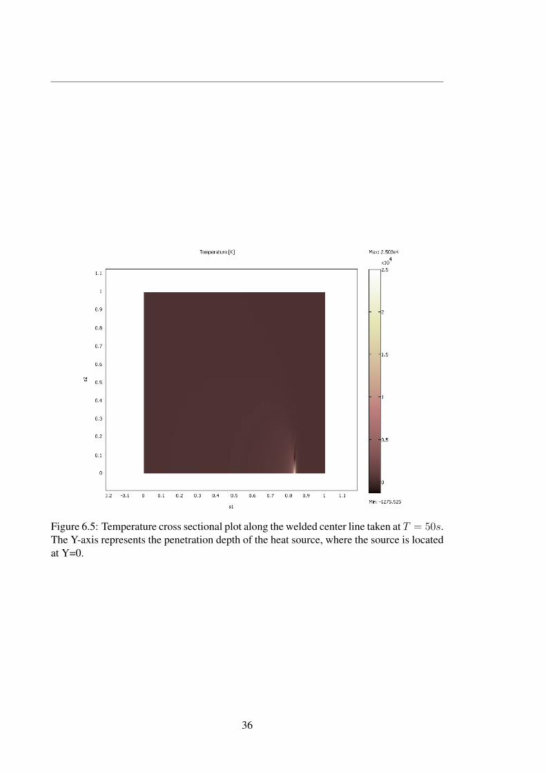
Figure 6.5: Temperature cross sectional plot along the welded center line taken at T = 50s.The Y-axis represents the penetration depth of the heat source, where the source is located
at Y=0.
36
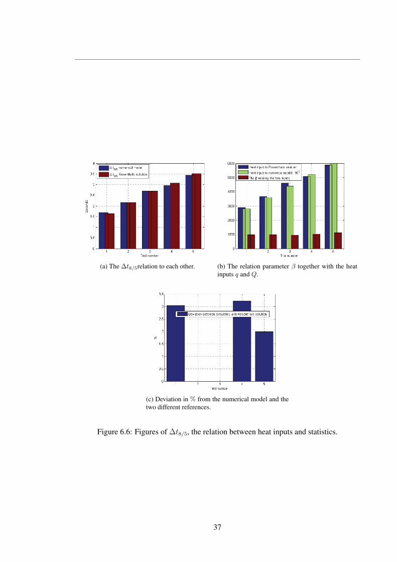
(a) The Δt8/5relation to each other. (b) The relation parameter β together with the heat
inputs q and Q.
(c) Deviation in % from the numerical model and the
two different references.
Figure 6.6: Figures of Δt8/5, the relation between heat inputs and statistics.
37


Chapter 7
Applying POD to the numericalFEM-model
The model developed in Chapter 6 is highly nonlinear, and has a complex nature. By
using the theory from Chapter 5, it is possible to minimize the number of states needed in
order to duplicate the response obtained in the nonlinear model. As earlier described, the
transition region Δt8/5 is important. In this chapter, the late response in the model is also
important, making it possible to monitor the initial temperature for the next pass.
7.1 Linearizing the modelThe following section used the same parameters as in Tab.6.1. The FEM-model was lin-
earized around a time t = t0, and exported to Matlab in the form
Mx = MAx+MBu
y = Cx+Du.(7.1)
The constraints (Dirichlet boundary conditions) were eliminated by writing the solution
vector U as
U = Nullx+ U0, (7.2)
where U0 is the linearization point, and Null is the null-space matrix for the constraints.
To make the case as realistic as possible, the output was measured in a point on the body
as seen in Fig.7.1, measuring the temperature as a function of time. When using the
parameters set in Chapter 6, the source will pass over the highlighted point in Fig.7.1 at
t0 = 30[s]. The point in blue represents the source and will in the FEM-model move at
a constant speed. When linearizing the model, one will make the point, representing the
source, stationary. Fig.7.1 represents the plate at t = 34[s].First, the general dynamics at the respective points in time were investigated. The
difference between the respective states at linearization points t0 = 31[s] and t0 = 33[s]are shown in Fig.7.2. Fig.C.1 represents the difference between the state matrix at two
other linearization points t = t0. It may be observed that the difference between the
states are very small, and in particular in the first 5200 states, which represents the 3D-
domain. Combining this with the fact that all the systems are stable, with eigenvalues
39
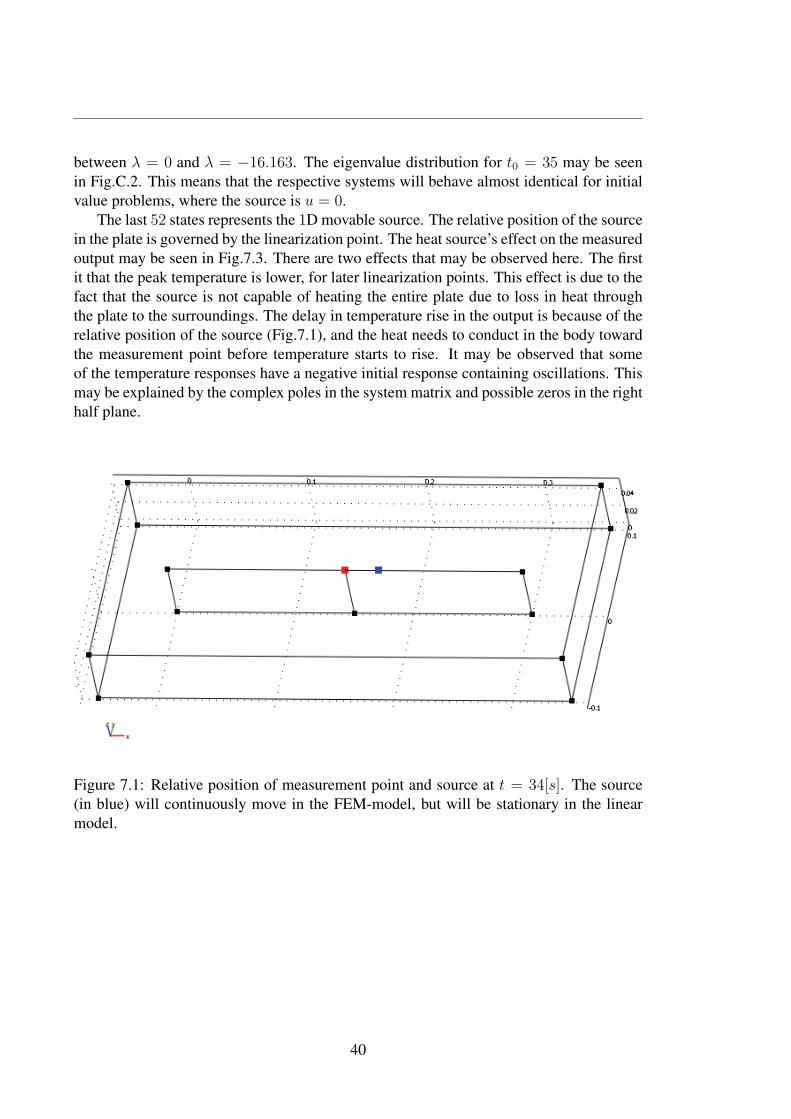
between λ = 0 and λ = −16.163. The eigenvalue distribution for t0 = 35 may be seen
in Fig.C.2. This means that the respective systems will behave almost identical for initial
value problems, where the source is u = 0.
The last 52 states represents the 1D movable source. The relative position of the source
in the plate is governed by the linearization point. The heat source’s effect on the measured
output may be seen in Fig.7.3. There are two effects that may be observed here. The first
it that the peak temperature is lower, for later linearization points. This effect is due to the
fact that the source is not capable of heating the entire plate due to loss in heat through
the plate to the surroundings. The delay in temperature rise in the output is because of the
relative position of the source (Fig.7.1), and the heat needs to conduct in the body toward
the measurement point before temperature starts to rise. It may be observed that some
of the temperature responses have a negative initial response containing oscillations. This
may be explained by the complex poles in the system matrix and possible zeros in the right
half plane.
Figure 7.1: Relative position of measurement point and source at t = 34[s]. The source
(in blue) will continuously move in the FEM-model, but will be stationary in the linear
model.
40
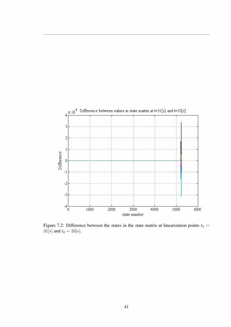
Figure 7.2: Difference between the states in the state matrix at linearization points t0 =31[s] and t0 = 33[s].
41
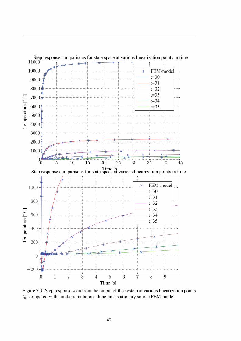
0 5 10 15 20 25 30 35 40 450
1000
2000
3000
4000
5000
6000
7000
8000
9000
10000
11000
Time [s]
Tem
per
ature
[◦C
]
Step response comparisons for state space at various linearization points in time
FEM-model
t=30
t=31
t=32
t=33
t=34
t=35
0 1 2 3 4 5 6 7 8 9
−200
0
200
400
600
800
1000
Time [s]
Tem
per
ature
[◦C
]
Step response comparisons for state space at various linearization points in time
FEM-model
t=30
t=31
t=32
t=33
t=34
t=35
Figure 7.3: Step response seen from the output of the system at various linearization points
t0, compared with similar simulations done on a stationary source FEM-model.
42
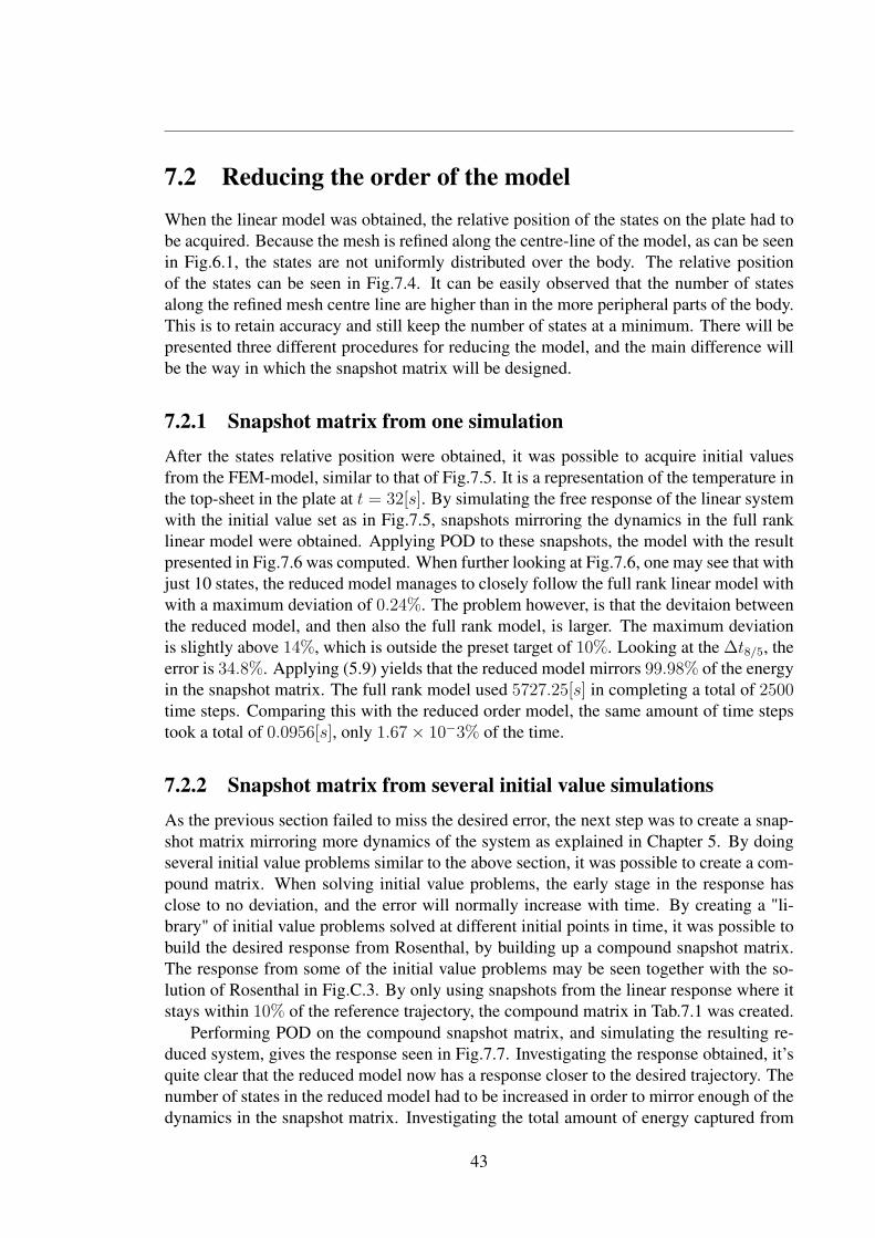
7.2 Reducing the order of the modelWhen the linear model was obtained, the relative position of the states on the plate had to
be acquired. Because the mesh is refined along the centre-line of the model, as can be seen
in Fig.6.1, the states are not uniformly distributed over the body. The relative position
of the states can be seen in Fig.7.4. It can be easily observed that the number of states
along the refined mesh centre line are higher than in the more peripheral parts of the body.
This is to retain accuracy and still keep the number of states at a minimum. There will be
presented three different procedures for reducing the model, and the main difference will
be the way in which the snapshot matrix will be designed.
7.2.1 Snapshot matrix from one simulationAfter the states relative position were obtained, it was possible to acquire initial values
from the FEM-model, similar to that of Fig.7.5. It is a representation of the temperature in
the top-sheet in the plate at t = 32[s]. By simulating the free response of the linear system
with the initial value set as in Fig.7.5, snapshots mirroring the dynamics in the full rank
linear model were obtained. Applying POD to these snapshots, the model with the result
presented in Fig.7.6 was computed. When further looking at Fig.7.6, one may see that with
just 10 states, the reduced model manages to closely follow the full rank linear model with
with a maximum deviation of 0.24%. The problem however, is that the devitaion between
the reduced model, and then also the full rank model, is larger. The maximum deviation
is slightly above 14%, which is outside the preset target of 10%. Looking at the Δt8/5, the
error is 34.8%. Applying (5.9) yields that the reduced model mirrors 99.98% of the energy
in the snapshot matrix. The full rank model used 5727.25[s] in completing a total of 2500time steps. Comparing this with the reduced order model, the same amount of time steps
took a total of 0.0956[s], only 1.67 × 10⁻³% of the time.
7.2.2 Snapshot matrix from several initial value simulationsAs the previous section failed to miss the desired error, the next step was to create a snap-
shot matrix mirroring more dynamics of the system as explained in Chapter 5. By doing
several initial value problems similar to the above section, it was possible to create a com-
pound matrix. When solving initial value problems, the early stage in the response has
close to no deviation, and the error will normally increase with time. By creating a "li-
brary" of initial value problems solved at different initial points in time, it was possible to
build the desired response from Rosenthal, by building up a compound snapshot matrix.
The response from some of the initial value problems may be seen together with the so-
lution of Rosenthal in Fig.C.3. By only using snapshots from the linear response where it
stays within 10% of the reference trajectory, the compound matrix in Tab.7.1 was created.
Performing POD on the compound snapshot matrix, and simulating the resulting re-
duced system, gives the response seen in Fig.7.7. Investigating the response obtained, it’s
quite clear that the reduced model now has a response closer to the desired trajectory. The
number of states in the reduced model had to be increased in order to mirror enough of the
dynamics in the snapshot matrix. Investigating the total amount of energy captured from
43
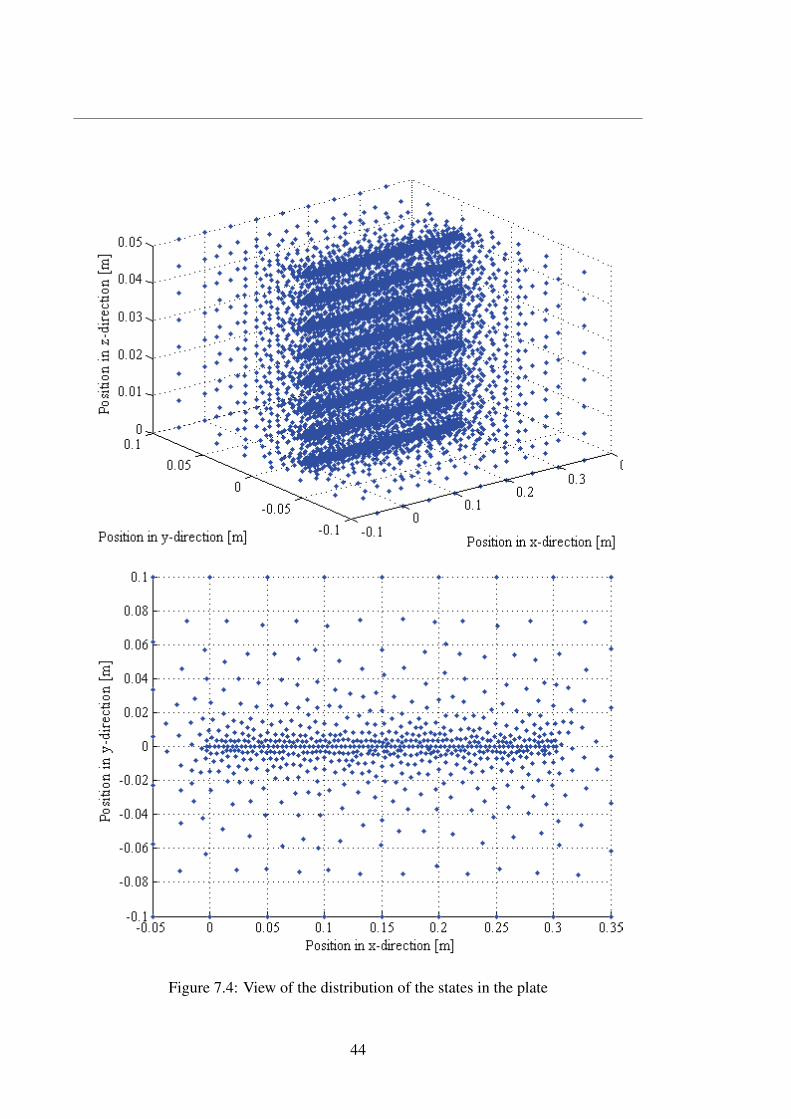
Figure 7.4: View of the distribution of the states in the plate
44

(a) xyz-view of initial temperature
(b) xz-view of initial temperature
Figure 7.5: Initial value in the top sheet of the plate at t = 32[s].
45
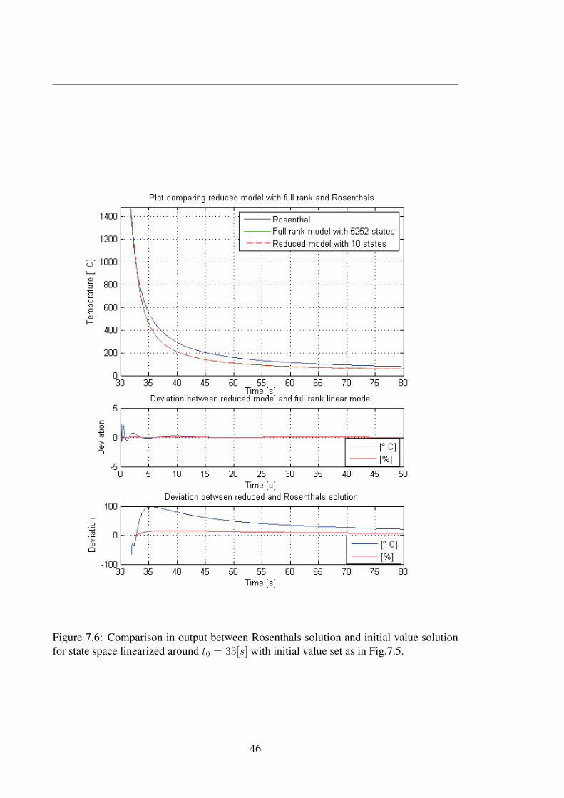
Figure 7.6: Comparison in output between Rosenthals solution and initial value solution
for state space linearized around t0 = 33[s] with initial value set as in Fig.7.5.
46
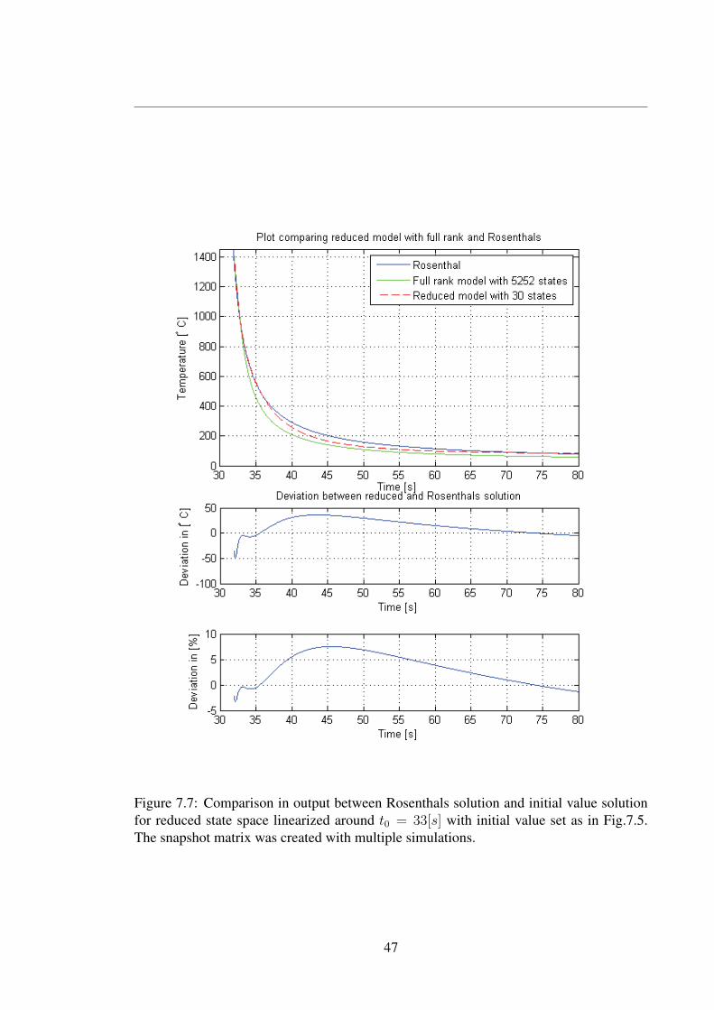
Figure 7.7: Comparison in output between Rosenthals solution and initial value solution
for reduced state space linearized around t0 = 33[s] with initial value set as in Fig.7.5.
The snapshot matrix was created with multiple simulations.
47
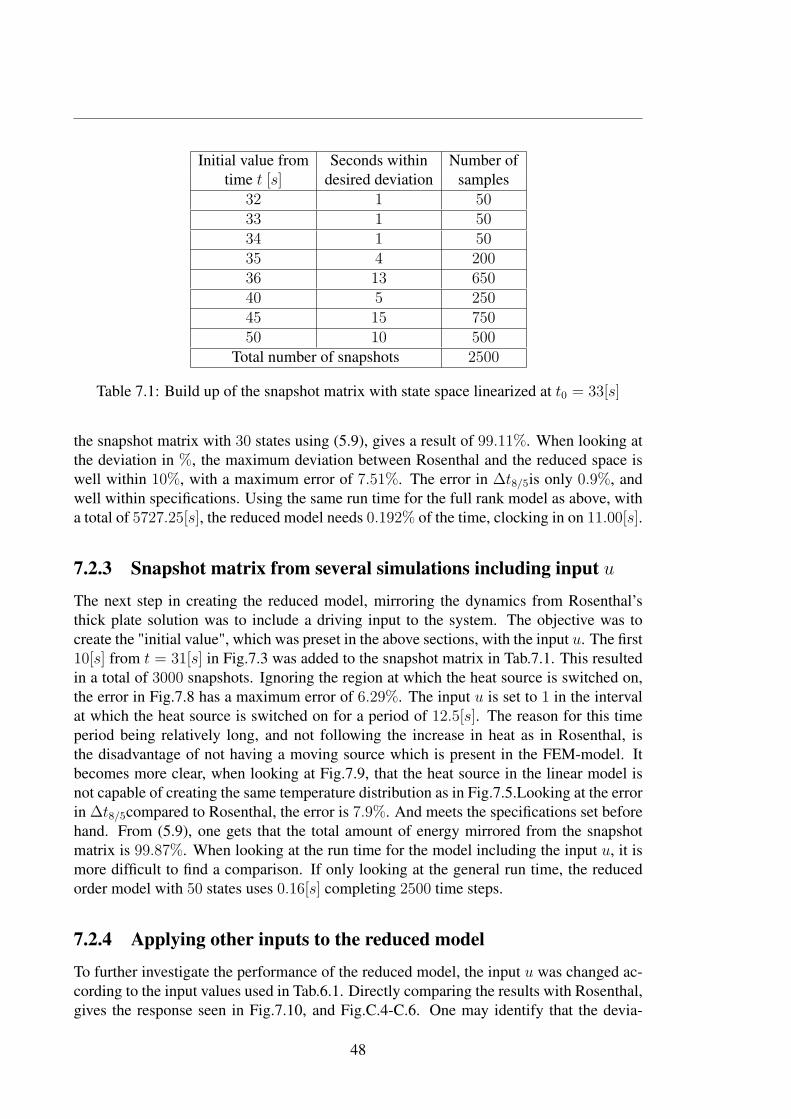
Initial value from Seconds within Number of
time t [s] desired deviation samples
32 1 5033 1 5034 1 5035 4 20036 13 65040 5 25045 15 75050 10 500
Total number of snapshots 2500
Table 7.1: Build up of the snapshot matrix with state space linearized at t0 = 33[s]
the snapshot matrix with 30 states using (5.9), gives a result of 99.11%. When looking at
the deviation in %, the maximum deviation between Rosenthal and the reduced space is
well within 10%, with a maximum error of 7.51%. The error in Δt8/5is only 0.9%, and
well within specifications. Using the same run time for the full rank model as above, with
a total of 5727.25[s], the reduced model needs 0.192% of the time, clocking in on 11.00[s].
7.2.3 Snapshot matrix from several simulations including input u
The next step in creating the reduced model, mirroring the dynamics from Rosenthal’s
thick plate solution was to include a driving input to the system. The objective was to
create the "initial value", which was preset in the above sections, with the input u. The first
10[s] from t = 31[s] in Fig.7.3 was added to the snapshot matrix in Tab.7.1. This resulted
in a total of 3000 snapshots. Ignoring the region at which the heat source is switched on,
the error in Fig.7.8 has a maximum error of 6.29%. The input u is set to 1 in the interval
at which the heat source is switched on for a period of 12.5[s]. The reason for this time
period being relatively long, and not following the increase in heat as in Rosenthal, is
the disadvantage of not having a moving source which is present in the FEM-model. It
becomes more clear, when looking at Fig.7.9, that the heat source in the linear model is
not capable of creating the same temperature distribution as in Fig.7.5.Looking at the error
in Δt8/5compared to Rosenthal, the error is 7.9%. And meets the specifications set before
hand. From (5.9), one gets that the total amount of energy mirrored from the snapshot
matrix is 99.87%. When looking at the run time for the model including the input u, it is
more difficult to find a comparison. If only looking at the general run time, the reduced
order model with 50 states uses 0.16[s] completing 2500 time steps.
7.2.4 Applying other inputs to the reduced model
To further investigate the performance of the reduced model, the input u was changed ac-
cording to the input values used in Tab.6.1. Directly comparing the results with Rosenthal,
gives the response seen in Fig.7.10, and Fig.C.4-C.6. One may identify that the devia-
48
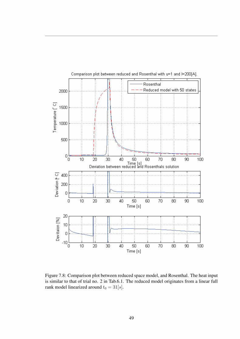
Figure 7.8: Comparison plot between reduced space model, and Rosenthal. The heat input
is similar to that of trial no. 2 in Tab.6.1. The reduced model originates from a linear full
rank model linearized around t0 = 31[s].
49
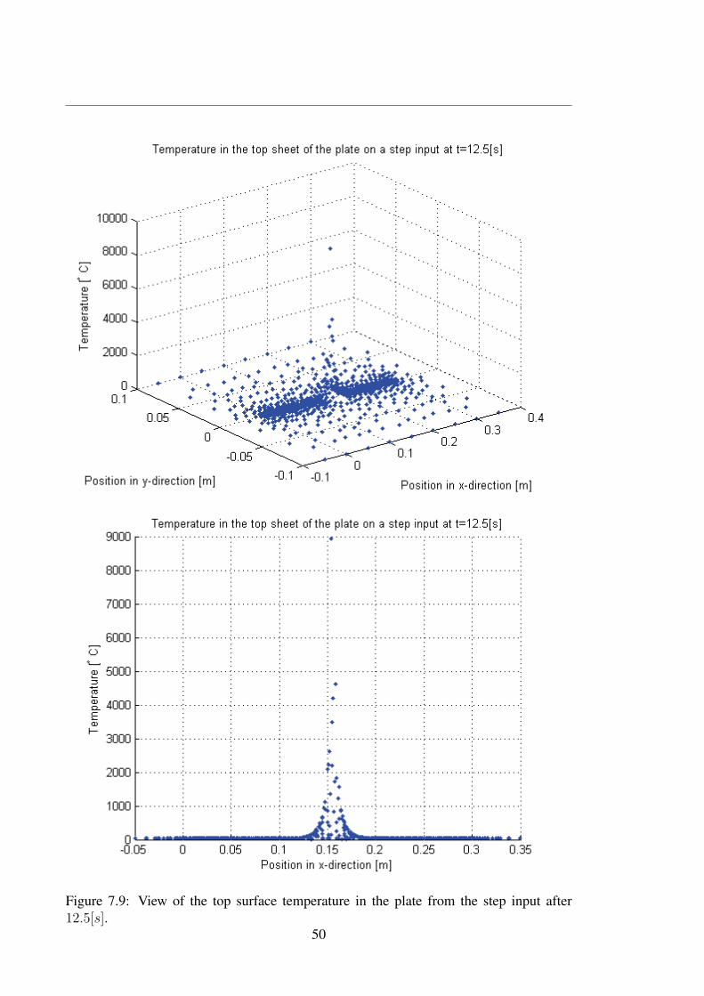
Figure 7.9: View of the top surface temperature in the plate from the step input after
12.5[s].50

tion in % is within 10% of the desired trajectory for all cases. The reason for why this
is possible, becomes clear when looking at Fig.C.7, showing the difference between the
states in two different state space models with linearization around t0 = 31[s] and different
heat inputs u. As one may see, the difference is only in the last 52 states representing the
1D-domain and the heat source as explained earlier in this chapter.
51
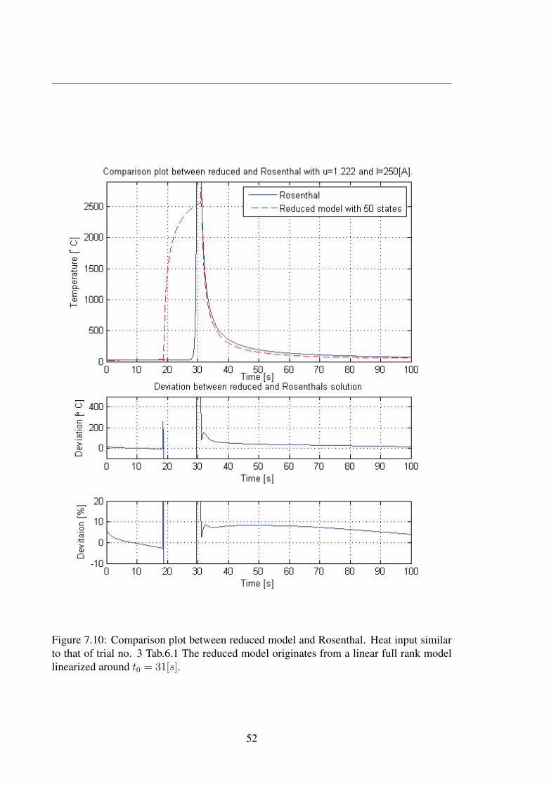
Figure 7.10: Comparison plot between reduced model and Rosenthal. Heat input similar
to that of trial no. 3 Tab.6.1 The reduced model originates from a linear full rank model
linearized around t0 = 31[s].
52
7.3 Discussion and evaluationThroughout this chapter, the progress in creating a reduced space model has been shown.
Looking at the reduced models performance, compared to the reference model deduced
by Rosenthal, it is quite clear that the linear model has problems in copying the correct
response. Looking at the full-rank linear model response in Fig.7.6, the temperature de-
creases too fast in the Δt8/5transition with an error of 14.1%. The same characteristics
repeat themselves in the reduced space.
By manipulating the content of the snapshot matrix, it was possible to lift the response
in order to decrease the error in Δt8/5. This was done without increasing the error in the
late response. In Fig.7.7 it is clear that the reduced space model no longer follows the full
rank linear model. As a paradox, increasing the number of states forces the response in the
Δt8/5-region closer to the full rank linear model. This is because the snapshot matrix does
not manage to completely copy the response of Rosenthal. If including enough energy in
the reduced model, the resulting response will come closer to the linear full rank model.
As a trade off, and because the main objective is to follow the response from Rosenthal,
the error between reduced and full rank linear model is accepted.
When further introducing the input u to the reduced model, another problem arise.
The property in the FEM-model of having a moving source gives rise to the good re-
creation of the response similar to Rosenthal. This property is not present in the linear
model. The source becomes stationary, and does not give the opportunity to create a
temperature distribution as in Fig.7.5. When linearizing around t0 = 31[s] as done for
the last sections in this chapter, the stationary source will make the initial value will look
like the one in Fig.7.9 after 12.5[s]. Reaching the point at which the sufficient amount
of heat was passed to the plate included an extensive amount of trial and error. If having
the source switched on for a shorter period of time, trying to exactly copy the Rosenthal
response, the decay in temperature is too high when comparing to Rosenthal. This will
introduce a major insecurity in the general performance of the model. In an online system,
it might prove difficult to recreate the response obtained with the heat input every time.
The tests performed here, show good results. However, there are no guarantees that the
stationary source will give a valid temperature distribution for every single case. Despite
the insecurities regarding the source, the model proves to have a good response for inputs
u outside the linearization point. The reason for this is as earlier described due to the fact
that the linearization of the FEM-model yields virtually the same linear full rank model for
two different heat-inputs linearized around the same point. This is shown in Fig.C.7. This
makes the method of creating this model versatile in the sense that it yields good response
for a large interval of inputs. When tested for the inputs in Tab.6.1, the deviation never
exceed 10% for the response after the heat source is turned off. It is natural that the error
is large in the region at which the heat source is switched on. This region will be neglected
when evaluating the error.
53


Chapter 8
Temperature experiments at AkerKværner Verdal
In this section the procedures for the experiments done at Aker Kværner Verdal (AKV)
will be shown. The test contains temperature measurements for welds performed with a
wide variety of parameters. The tests were performed within specified procedures worked
out at AKV shown in (Helden & Dreyer 1999). The experiments where performed as part
of the development of an automated temperature control-system. The measurements will
be used as decision parameters when controlling the Δt8/5 in the welded specimen.
8.1 Test rig and set upThe setup for the test consisted of the following and can be seen in Fig.8.1:
• ThermaCAMTM S65 infrared camera
• Fujitsu Siemens lifebook laptop computer with FireWire interface
• Structural steel sheet with measures 1100mm× 800mm× 50mm
• IRB2400L ABB 6DOF robotic welding manipulator
• Camera tripod mount
8.2 Test proceduresPrevious to the tests, a test plan was prepared. The objective of the test plan was to span
the entire temperature- and input parameters-interval encountered during normal welding.
The tests were divided into sessions, and there were done a total of 8 sessions. Each session
was designed to stress relevant settings at distinct situations. To test the consistency and
accuracy of Δt8/5, the analytical solution of Rosenthal (3.10) was used as a reference, and
is referred to as the Calculated solution. The camera was set up according to (FLI 2006)
and resulted in Tab.8.1.
55

Figure 8.1: The rig set-up, with the camera in front, the steel plate on the work bench and
the manipulator behind.
Object parametersObject External optics Atmosphere
Ses
sion
no.
Em
issi
vit
yε
Dis
tance
[m]
Refl
ecte
dte
mp.
[◦C
]
Tem
per
ature
[◦C
]
Tra
nsm
issi
on
Atm
osp
her
icte
mp.
[◦C
]
Rel
ativ
ehum
idit
y%
1 0.92 0.9 20 15 1.00 15 502 0.92 0.9 20 15 1.00 15 503 0.92 0.9 20 15 1.00 15 504 0.92 0.9 20 12 1.00 12 505 0.92 0.9 20 12 1.00 12 506 0.92 0.85 20 13 1.00 13 507 0.92 0.85 20 13 1.00 13 508 0.92 0.85 20 13 1.00 13 50
Table 8.1: Object parameters set in the camera for the different sessions
56

8.2.1 Session 1A total of four strings were done, where the inter-pass temperature in each consecutive
pass was 40◦C in average along the centre-line. The strings were lay beside each other,
and each string was 200mm. The reason for the initial temperature being 15◦C on the first
string, was that the plate was at room temperature. The session was done with a weaving
of 2 mm, which will make the string wider, and the resultant heat distribution will be less
equal to that of a point source. This will introduce more uncertainties in the measurements
compared to the reference calculated temperature.
Str
ing
no.
Curr
ent
[A]
Volt
age
[V]
Wel
dsp
eed
[mm/s
]
Init
ial
tem
p.
[◦C
]
Mea
sure
dΔt 8
/5
Cal
cula
ted
Δt 8
/5
Dev
iati
on
[%]
1 240 26 8 15 2.90 1.76 64.772 275 29 9 40 3.81 2.17 75.443 275 29 8 40 4.28 2.44 74.864 260 27.75 8 40 3.64 2.21 64.37
Average deviation 69.87
8.2.2 Session 2The session was completed with the same characteristics as in session 1 and with the
parameters shown in the table below.
Str
ing
no.
Curr
ent
[A]
Volt
age
[V]
Wel
dsp
eed
[mm/s
]
Init
ial
tem
p.
[◦C
]
Mea
sure
dΔt 8
/5
Cal
cula
ted
Δt 8
/5
Dev
iati
on
[%]
1 250 28 9 15 2.99 1.97 51.572 250 28 6 40 4.35 2.86 51.853 254 28 6 40 4.36 2.91 49.984 254 28 6 40 4.53 2.91 55.89
Average deviation 52.33
8.2.3 Session 3The plate was preheated with heating elements. This was done in order to simulate a multi-
pass environment. By installing heating elements on the work piece, it was possible to
manipulate the initial temperature in the plate beyond room temperature and temperature
57
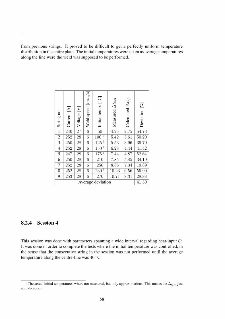
from previous strings. It proved to be difficult to get a perfectly uniform temperature
distribution in the entire plate. The initial temperatures were taken as average temperatures
along the line were the weld was supposed to be performed.S
trin
gno.
Curr
ent
[A]
Volt
age
[V]
Wel
dsp
eed
[mm/s
]
Init
ial
tem
p.
[◦C
]
Mea
sure
dΔt 8
/5
Cal
cula
ted
Δt 8
/5
Dev
iati
on
[%]
1 240 27 6 50 4.25 2.75 54.732 252 28 6 100 1 5.42 3.61 50.203 250 28 6 125 1 5.53 3.96 39.794 252 28 6 150 1 6.28 4.44 41.425 247 28 6 175 1 7.44 4.87 52.646 250 28 6 210 7.85 5.85 34.197 252 28 6 250 8.86 7.34 19.898 252 28 6 230 1 10.23 6.56 55.909 253 28 6 270 10.71 8.31 28.88
Average deviation 41.30
8.2.4 Session 4
This session was done with parameters spanning a wide interval regarding heat-input Q.
It was done in order to complete the tests where the initial temperature was controlled, in
the sense that the consecutive string in the session was not performed until the average
temperature along the centre-line was 40 ◦C.
1The actual initial temperatures where not measured, but only approximations. This makes the Δt8/5 just
an indication.
58

Str
ing
no.
Curr
ent
[A]
Volt
age
[V]
Wel
dsp
eed
[mm/s
]
Init
ial
tem
p.
[◦C
]
Mea
sure
dΔt 8
/5
Cal
cula
ted
Δt 8
/5
Dev
iati
on
[%]
1 202 25.3 6 15 3.15 1.92 64.352 223 26.5 6 40 3.66 2.41 51.353 249 27.5 6 40 4.16 2.80 48.464 274 28.8 6 40 5.02 3.22 55.735 296 30.0 6 40 6.055 3.63 66.636 200 25.3 8 40 2.05 1.55 32.267 226 26.5 8 40 2.79 1.84 51.798 245 27.0 8 40 3.18 2.03 56.509 273 28.5 8 40 4.04 2.39 68.9810 300 30.0 8 40 5.02 2.76 81.63
Average deviation 57.77
0 10 20 30 40 50
200
400
600
800
1000
1200
1400
1600
Time [s]
Tem
per
ature
[◦C
]
Comparison plot with initial temperature 40[◦C]
Measured temperature
Temperature from Rosenthal
Figure 8.2: Comparison between Rosenthal and weld no.5 from session 4.
59
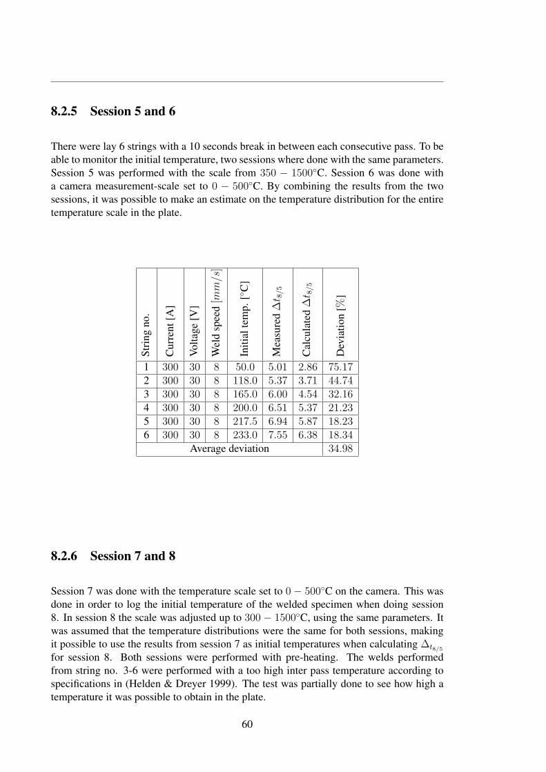
8.2.5 Session 5 and 6
There were lay 6 strings with a 10 seconds break in between each consecutive pass. To be
able to monitor the initial temperature, two sessions where done with the same parameters.
Session 5 was performed with the scale from 350 − 1500◦C. Session 6 was done with
a camera measurement-scale set to 0 − 500◦C. By combining the results from the two
sessions, it was possible to make an estimate on the temperature distribution for the entire
temperature scale in the plate.
Str
ing
no.
Curr
ent
[A]
Volt
age
[V]
Wel
dsp
eed
[mm/s
]
Init
ial
tem
p.
[◦C
]
Mea
sure
dΔt 8
/5
Cal
cula
ted
Δt 8
/5
Dev
iati
on
[%]
1 300 30 8 50.0 5.01 2.86 75.172 300 30 8 118.0 5.37 3.71 44.743 300 30 8 165.0 6.00 4.54 32.164 300 30 8 200.0 6.51 5.37 21.235 300 30 8 217.5 6.94 5.87 18.236 300 30 8 233.0 7.55 6.38 18.34
Average deviation 34.98
8.2.6 Session 7 and 8
Session 7 was done with the temperature scale set to 0 − 500◦C on the camera. This was
done in order to log the initial temperature of the welded specimen when doing session
8. In session 8 the scale was adjusted up to 300 − 1500◦C, using the same parameters. It
was assumed that the temperature distributions were the same for both sessions, making
it possible to use the results from session 7 as initial temperatures when calculating Δt8/5
for session 8. Both sessions were performed with pre-heating. The welds performed
from string no. 3-6 were performed with a too high inter pass temperature according to
specifications in (Helden & Dreyer 1999). The test was partially done to see how high a
temperature it was possible to obtain in the plate.
60
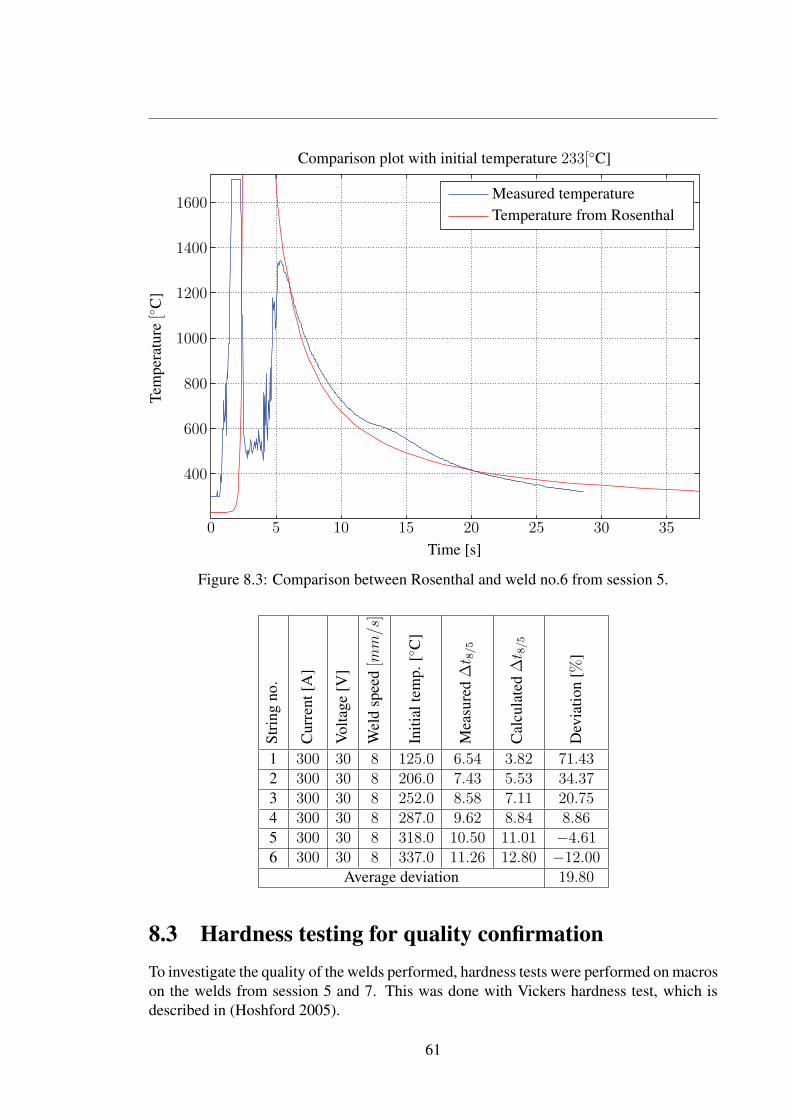
0 5 10 15 20 25 30 35
400
600
800
1000
1200
1400
1600
Time [s]
Tem
per
ature
[◦C
]Comparison plot with initial temperature 233[◦C]
Measured temperature
Temperature from Rosenthal
Figure 8.3: Comparison between Rosenthal and weld no.6 from session 5.
Str
ing
no.
Curr
ent
[A]
Volt
age
[V]
Wel
dsp
eed
[mm/s
]
Init
ial
tem
p.
[◦C
]
Mea
sure
dΔt 8
/5
Cal
cula
ted
Δt 8
/5
Dev
iati
on
[%]
1 300 30 8 125.0 6.54 3.82 71.432 300 30 8 206.0 7.43 5.53 34.373 300 30 8 252.0 8.58 7.11 20.754 300 30 8 287.0 9.62 8.84 8.865 300 30 8 318.0 10.50 11.01 −4.616 300 30 8 337.0 11.26 12.80 −12.00
Average deviation 19.80
8.3 Hardness testing for quality confirmationTo investigate the quality of the welds performed, hardness tests were performed on macros
on the welds from session 5 and 7. This was done with Vickers hardness test, which is
described in (Hoshford 2005).
61
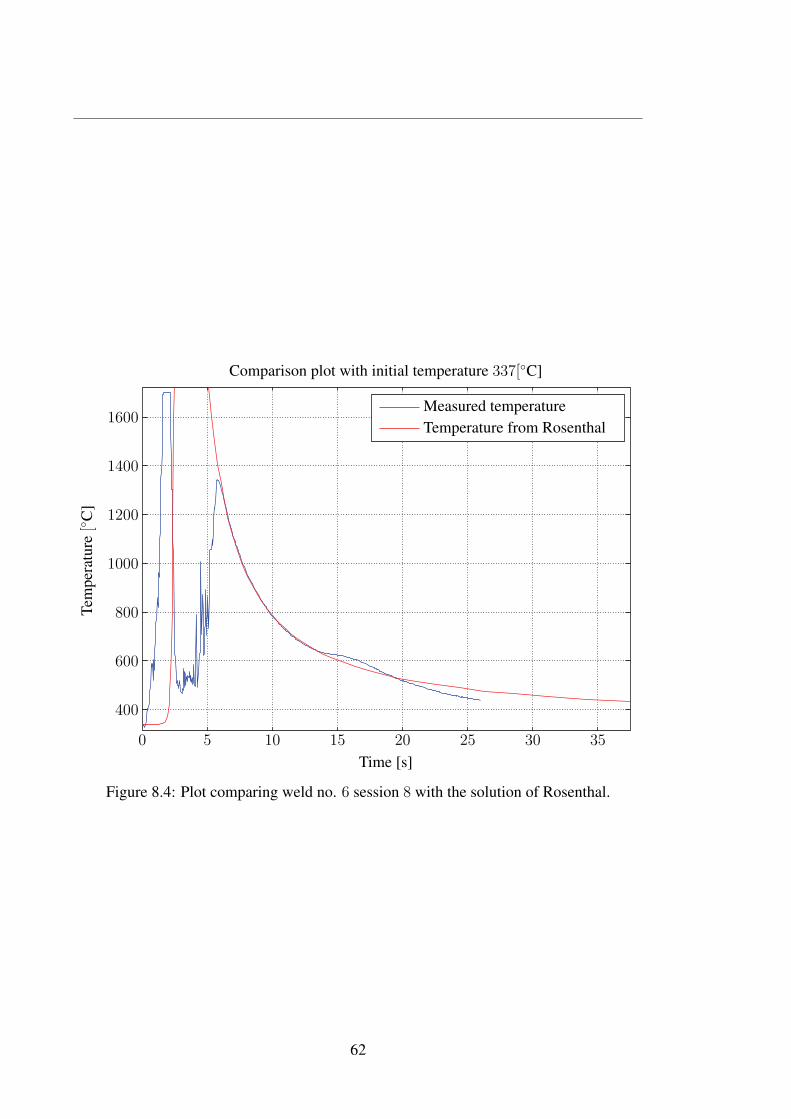
0 5 10 15 20 25 30 35
400
600
800
1000
1200
1400
1600
Time [s]
Tem
per
ature
[◦C
]
Comparison plot with initial temperature 337[◦C]
Measured temperature
Temperature from Rosenthal
Figure 8.4: Plot comparing weld no. 6 session 8 with the solution of Rosenthal.
62

8.3.1 Quick review of Vickers hardness testThe test-rig uses a diamond shaped as a square pyramid, with an angle of 136◦ between
opposite faces as an indenter Fig.8.5. The footprint made by the indenter is geometrically
independent of the load applied to the material measured. The Vickers pyramid number
(Hv) is then determined by the ratio F/A where F is force applied and A is the area made
by the indentation. A is determined by
A =d2
2sin(136◦/2)
A ≈ d2
1.854,
(8.1)
where d is the average length of d1 and d2 in Fig.8.5. This then gives rise to the number
measuring hardness,
Hv =F
A≈ 1.854F
d2
[kgf
mm2
]. (8.2)
This is then converted to SI-units and 1kgf/mm2 = 9.80665 × 10⁶Pa. When testing
the hardness of the weld, one probes the points from 1-20 as shown in Fig.8.6. The re-
quirements for steel in applications used in for example sub-sea installations, are hardness
values Hv below 325. The hardness number will be highest in the transition between the
base material and the HAZ, and will thus be the most critical regions.
8.3.2 Results from Vickers hardness testThe results from the hardness tests are summarized in Tab.E.1 and Tab.E.2. When looking
at Fig.8.6, there is a total of 16 points to be probed. Because the welds were laid side by
side with no space in between, the points close to the weld’s surface are heat-affected by
the subsequent string. This makes the hardness tested in the regions from point 1 − 7 and
15 − 16 not valid, and thus not tested. When looking at the tables in Appendix E, it may
be concluded that all the welds are well within the demands for hardness in welds.
8.4 DiscussionThe results in this chapter are obtained through Infra-red measurements of a steel plate
at which welding with different parameters has been performed. The ultimate goal from
the tests was to investigate the possibility to use the infra red camera to measure the tem-
perature in the welded specimen, and use this information to control the Δt8/5 in a multi
pass welding environment. In order to draw any conclusions, a wide variety of trials were
performed. This was done in order to stress relevant situations in a common welding set-
ting. The tests were performed according to the tables seen in Section 8.2.1 through to
8.2.6. There will be put less emphasis on the two first sessions due to the use of weaving
during welding. Weaving makes the heat source less equal to a point source, making the
calculated solution invalid. The results from the two sessions are only presented as an
indication.
63
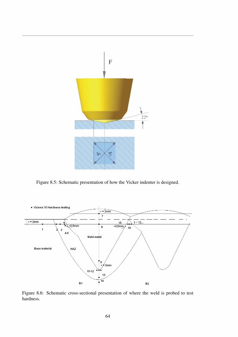
Figure 8.5: Schematic presentation of how the Vicker indenter is designed.
Figure 8.6: Schematic cross-sectional presentation of where the weld is probed to test
hardness.
64
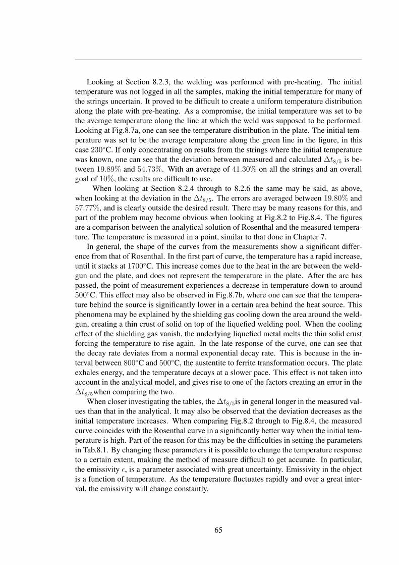
Looking at Section 8.2.3, the welding was performed with pre-heating. The initial
temperature was not logged in all the samples, making the initial temperature for many of
the strings uncertain. It proved to be difficult to create a uniform temperature distribution
along the plate with pre-heating. As a compromise, the initial temperature was set to be
the average temperature along the line at which the weld was supposed to be performed.
Looking at Fig.8.7a, one can see the temperature distribution in the plate. The initial tem-
perature was set to be the average temperature along the green line in the figure, in this
case 230◦C. If only concentrating on results from the strings where the initial temperature
was known, one can see that the deviation between measured and calculated Δt8/5 is be-
tween 19.89% and 54.73%. With an average of 41.30% on all the strings and an overall
goal of 10%, the results are difficult to use.
When looking at Section 8.2.4 through to 8.2.6 the same may be said, as above,
when looking at the deviation in the Δt8/5. The errors are averaged between 19.80% and
57.77%, and is clearly outside the desired result. There may be many reasons for this, and
part of the problem may become obvious when looking at Fig.8.2 to Fig.8.4. The figures
are a comparison between the analytical solution of Rosenthal and the measured tempera-
ture. The temperature is measured in a point, similar to that done in Chapter 7.
In general, the shape of the curves from the measurements show a significant differ-
ence from that of Rosenthal. In the first part of curve, the temperature has a rapid increase,
until it stacks at 1700◦C. This increase comes due to the heat in the arc between the weld-
gun and the plate, and does not represent the temperature in the plate. After the arc has
passed, the point of measurement experiences a decrease in temperature down to around
500◦C. This effect may also be observed in Fig.8.7b, where one can see that the tempera-
ture behind the source is significantly lower in a certain area behind the heat source. This
phenomena may be explained by the shielding gas cooling down the area around the weld-
gun, creating a thin crust of solid on top of the liquefied welding pool. When the cooling
effect of the shielding gas vanish, the underlying liquefied metal melts the thin solid crust
forcing the temperature to rise again. In the late response of the curve, one can see that
the decay rate deviates from a normal exponential decay rate. This is because in the in-
terval between 800◦C and 500◦C, the austentite to ferrite transformation occurs. The plate
exhales energy, and the temperature decays at a slower pace. This effect is not taken into
account in the analytical model, and gives rise to one of the factors creating an error in the
Δt8/5when comparing the two.
When closer investigating the tables, the Δt8/5is in general longer in the measured val-
ues than that in the analytical. It may also be observed that the deviation decreases as the
initial temperature increases. When comparing Fig.8.2 through to Fig.8.4, the measured
curve coincides with the Rosenthal curve in a significantly better way when the initial tem-
perature is high. Part of the reason for this may be the difficulties in setting the parameters
in Tab.8.1. By changing these parameters it is possible to change the temperature response
to a certain extent, making the method of measure difficult to get accurate. In particular,
the emissivity ε, is a parameter associated with great uncertainty. Emissivity in the object
is a function of temperature. As the temperature fluctuates rapidly and over a great inter-
val, the emissivity will change constantly.
65
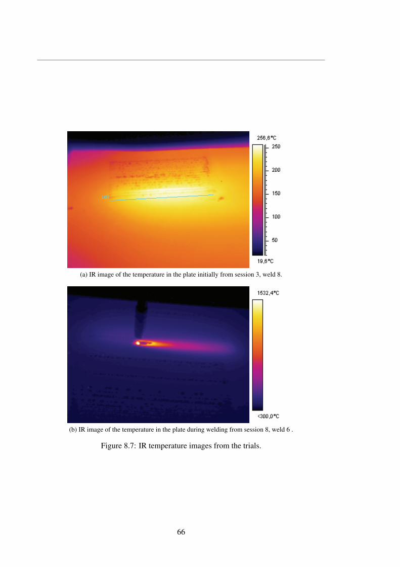
(a) IR image of the temperature in the plate initially from session 3, weld 8.
(b) IR image of the temperature in the plate during welding from session 8, weld 6 .
Figure 8.7: IR temperature images from the trials.
66
Chapter 9
Conclusion
In this project there has been constructed a numerical mathematical model describing the
complex nature of the partial differential equations governing the process of heat flow in
steel plates.
The model itself was made in Chapter 6 with the FEM and compared to the thick plate
solution of Rosenthal. Through consistency testing of the numerical model, it was estab-
lished a relation between the model and the reference. As an initial goal, a temperature
decay rate between 800◦C and 500 ◦C within 10% of the reference model was set. This
goal was reached with good margins. The maximum error being found to 3.22%, shows
that results obtained are well within the scope of the project. This was done despite the
fact that the model did not meet the semi-infinite body requirement.
In Chapter 7 the numerical model was put under the method of model reduction, which
goal was to recreate the results above with the same goal regarding error. By optimizing
the inputs to the linear system, a reduced model was possible to obtain with good perfor-
mance. Through the tests performed, the reduced model, made with the compound matrix
in Tab.7.1, managed to recreate the Δt8/5region with a maximum error of 0.9%. This is
very good, even when comparing to the FEM-model from which the reduced model origi-
nates from. When input u was included into the system, problems regarding the heat input
to the system arise. Only through extensive trial and error was it made possible to create
an adequate response in the relevant regions. This makes the system vulnerable when used
in an automated system, possibly making the wrong decisions if relying on the models
response. The general dynamics in the system however, shows great adaptation, and is
able to cope with a wide variety of inputs without introducing large errors. The results are
promising, and through more research in modelling the heat-source, it should be possible
to use the reduced model in an automated welding system.
When looking at the results obtained in Chapter 8, there are large errors present when
comparing to the reference Δt8/5. This then leads to the fact that at the moment, the
measurements are not accurate enough to be used as a decision parameter in an automated
welding system. However, the results show consistency, and with more tuning on the
object parameters and identifying errors in the set up, it is possible to use this method in
an automated system. It may also be concluded that the accuracy improved as the initial
temperature of the welded specimen increased.
In order to create an automated welding system working under optimal conditions,
67

this project has found a possible entrance to the path completing the task. It still remains
a huge amount work before it can be realized in a live environment.
9.1 Future workTo further close in on the ultimate goal of the project, there are a number of steps to be
completed.
• Model a more reliable heat-source creating a temperature distribution in the welded
specimen more equal to that of Rosenthal.
• Investigate the errors present in the IR-measurements and reduce the overall error
making them suitable as decision parameters.
• Incorporate the reduced model in a closed loop temperature control system, control-
ling the Δt8/5.
• Test the entire system in a live environment.
68
Bibliography
Astrid, P. (2004), Reduction of Process Simulation Models: a proper orthogonal decom-
position approach, PhD thesis, Technische Universiteit Eindhoven.
Camp, K. A. E. & King, B. B. (1997), ‘A comparison of balanced truncation techniques
for reduced order controllers’.
URL: citeseer.ist.psu.edu/570217.html"
Cazemier, W. (1997), ‘Proper orthogonal decomposition and low dimensional models for
turbulent flows’.
URL: http://irs.ub.rug.nl/ppn/161483305
Com (2005), Comsol Multiphysics User’s Guide version 3.2.
FLI (2006), ThermaCAMTM S65 User’s manual, a156 edn.
Grong, . (1994), Metallurgical Modelling of Welding, The Institute of Materials.
Gugercin, S., Antoulas, A. C. & Beattie, C. A. (2004), ‘First-order conditions and an
iterative rational krylov algorithm for optimal H2 model reduction’, Technical report .
Gugercin, S. & Wilcox, K. (2007), ‘Krylov projection framework for fourier model reduc-
tion’, provisionally accepted in Automatica p. 7.
Helden, P. O. & Dreyer, P. H. (1999), Plate- og Sveise Håndbok, Sveiseteknisk avdeling.
Hoshford, W. F. (2005), Mechanical behavior of materials, Cambridge University Press.
Hovland, S. & Gravdahl, J. T. (2006), ‘Order reduction and output feedback stabilization
of an unstable cfd model’, American Control Conference. Minneapolis, Minnesota .
Jiluan, P. (2003), Arc Welding Control, Vol. Developments in heat transfer vol. 14, Wood-
head Publishing Limited, England.
Karhunen, K. (1946), ‘Zur spektral theorie stochasticher prozesse’, Ann. Acad. Sci. Fenni-cae, Ser. A1 Math Phys 34, 1–7.
Loève, M. (1946), ‘Functions aleatoire de second ordre’, Revue science 84, 195–206.
Nguyen, N. (2004), Thermal Analysis of welds, WIT Press.
69

Olsson, K. H. A. (2002), Model order reduction in femlab by dual rational arnoldi, Mas-
ter’s thesis, Göteborg university.
Pires, J. N., Loureiro, A. & Bolmsjö, G. (2006), Welding Robots : technology, systemissues and applications, Springer-Verlag London Limited.
Reddy, J. N. (2006), An Introduction to the Finite Element Method, McGraw-Hill.
Willcox, K. & Megretski, A. (2005), ‘Fourier model reduction for large-scale applications
in computational fluid dynamics’, SIAM, Journal on Scientific Computing Vol. 26, No.3, 944–962.
70

Appendices
71

Appendix A
Modelling of a single-pass weld
Procedure when creating the model describing a single pass weld in a 50mm thick plate.
This procedure was done individually for each heat-input to the model in order to get a
different temperature response.
A.1 Application modes and modules used in the model• A 3D model which physical properties are heat transfer by conduction.
• A 1D model which is in a weak time dependent form.
A.2 Constants used in the modelName Expression Description
u_weld 0.005 Welding speed [m/s]T0 300 Initial temperature in the plate [K]Q 3.6 × 10⁶ Heat input [W/m3]State 1 Heat source on/off
72

A.3 Geometries in the model1. 3D model:
Figure A.1: 3D model geometry. Dimensions: 400 × 200 × 50[mm]
73
2. 1D model:
Figure A.2: 1D model geometry. Dimension: 1[mm]
A.4 Geometry 1, 3D
Description of the 3D model parameters and settings.
A.4.1 Mesh statisticsNumber of degrees of freedom 5253Number of edge elements 257Number of boundary elements 3268Number of elements 8890Minimum element quality 0.256
A.4.2 Application mode:Heat Transfer by Conduction (ht)
Application mode type: Heat Transfer by Conduction Application mode name: ht
Application Mode Properties
Property ValueDefault element type Lagrange - Linear
Analysis type Transient
Frame Reference frame
Weak constraints Off
74

Figure A.3: Meshed 3D geometry
Variables
The variable for which the problem is solved for, is the temperature T.
Boundary Settings
All the boundaries in the model were set to thermal insulation.
Subdomain settings
The model was made in steel, AISI 4340. The following properties of the material was
used in the model:Thermal conductivity (k) W
m · K44.5
Density (rho) kgm3 7850
Heat capacity (C) Jkg · K
475
A.5 Geometry 2, 1D
Description of the 1D model and its parameters.
A.5.1 Scalar Expressions
Name Expressionk_abs 8 ∗ 103 − 10(T − 300)u_abs k_abs ∗ u
75
A.5.2 Mesh statistics
The following mesh statistics are contained in the 1D-domain:
Number of mesh points 27Number of elements 27Number of boundary elements 1.0Element length ratio 0.159
Boundary 1 2Maximum element size - 10−5
Element growth rate - 1.1
A.5.3 Application Mode: Weak Form, Subdomain w
Application mode type: Weak Form, Subdomain.
Application mode name:w
Application Mode Properties
Property ValueDefault element type Lagrange - Quadratic
Wave extension Off
Frame Reference frame
Weak constraints Off
Variables
Dependent variables:u, u_tShape functions: shlag(2,′u′)Interior boundaries are not active.
Point Settings
Point 1 2constr term (constr) 0 1 − ustyle {0, {0, 0, 0}} {0, {0, 0, 255}}
Subdomain Settings
Subdomain 1weak term (ux− u_abs) ∗ State ∗ u_test+Q ∗ T_testdweak term 0
Subdomain initial value 1u 1
76
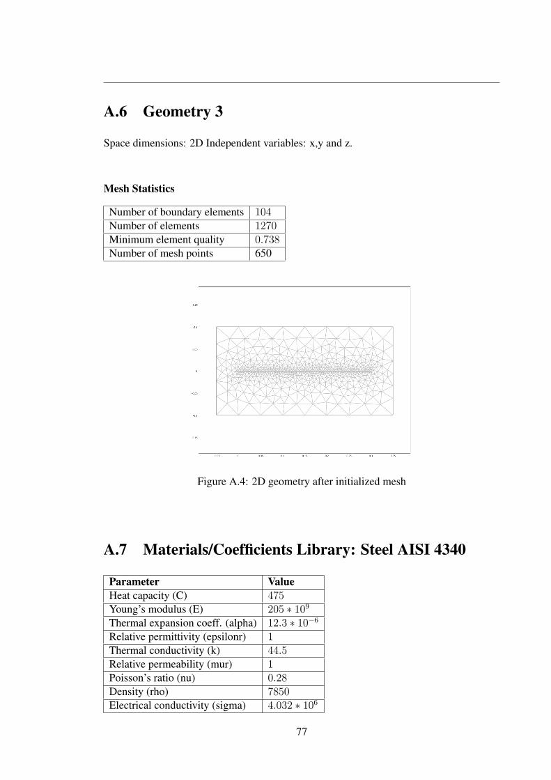
A.6 Geometry 3
Space dimensions: 2D Independent variables: x,y and z.
Mesh Statistics
Number of boundary elements 104Number of elements 1270Minimum element quality 0.738Number of mesh points 650
Figure A.4: 2D geometry after initialized mesh
A.7 Materials/Coefficients Library: Steel AISI 4340
Parameter ValueHeat capacity (C) 475Young’s modulus (E) 205 ∗ 109
Thermal expansion coeff. (alpha) 12.3 ∗ 10−6
Relative permittivity (epsilonr) 1Thermal conductivity (k) 44.5Relative permeability (mur) 1Poisson’s ratio (nu) 0.28Density (rho) 7850Electrical conductivity (sigma) 4.032 ∗ 106
77

A.8 Extrusion Coupling Variables: Geom 1, Source Sub-domain: 1
Name ValueExpression TTransformation type General
Source transformation x, y, zDestination Subdomain 1 (Geom2) u_weld ∗ t, 0, x
A.9 Solver Parameters
Analysis type Transient
Auto select solver On
Solver Time dependent
Solution form Automatic
Symmetric Off
Adaption Off
A.9.1 Direct(UMFPACK)
Solver type: Linear system solver.
Parameter ValuePivot threshold 0.1Memory allocation factor 0.7
A.9.2 Time Stepping
Parameter ValueRelative tolerance 0.01Absolute tolerance 1Times to store in output Specified times
Time steps taken by solver Free
Initial time step 0.0010Maximum time step 1.0Maximum BDF order 5Singular mass matrix Maybe
Consistent initialization of DAE systems Backward Euler
Error estimation strategy Include algebraic
Allow complex numbers Off
78
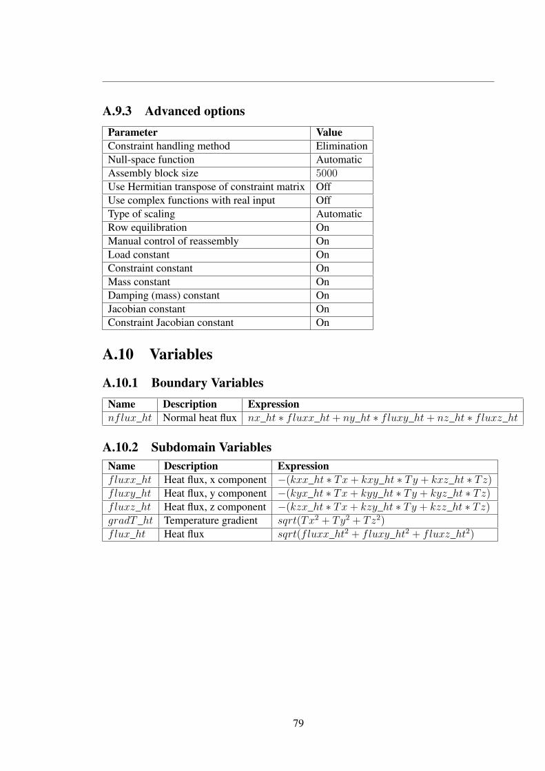
A.9.3 Advanced optionsParameter ValueConstraint handling method Elimination
Null-space function Automatic
Assembly block size 5000Use Hermitian transpose of constraint matrix Off
Use complex functions with real input Off
Type of scaling Automatic
Row equilibration On
Manual control of reassembly On
Load constant On
Constraint constant On
Mass constant On
Damping (mass) constant On
Jacobian constant On
Constraint Jacobian constant On
A.10 Variables
A.10.1 Boundary VariablesName Description Expressionnflux_ht Normal heat flux nx_ht ∗ fluxx_ht+ ny_ht ∗ fluxy_ht+ nz_ht ∗ fluxz_ht
A.10.2 Subdomain VariablesName Description Expressionfluxx_ht Heat flux, x component −(kxx_ht ∗ Tx+ kxy_ht ∗ Ty + kxz_ht ∗ Tz)fluxy_ht Heat flux, y component −(kyx_ht ∗ Tx+ kyy_ht ∗ Ty + kyz_ht ∗ Tz)fluxz_ht Heat flux, z component −(kzx_ht ∗ Tx+ kzy_ht ∗ Ty + kzz_ht ∗ Tz)gradT_ht Temperature gradient sqrt(Tx2 + Ty2 + Tz2)flux_ht Heat flux sqrt(fluxx_ht2 + fluxy_ht2 + fluxz_ht2)
79

Appendix B
Figures relevant for Chapter 6
81
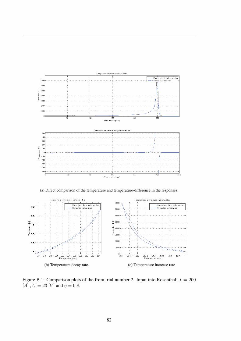
(a) Direct comparison of the temperature and temperature-difference in the responses.
(b) Temperature decay rate. (c) Temperature increase rate
Figure B.1: Comparison plots of the from trial number 2. Input into Rosenthal: I = 200[A] , U = 23 [V ] and η = 0.8.
82
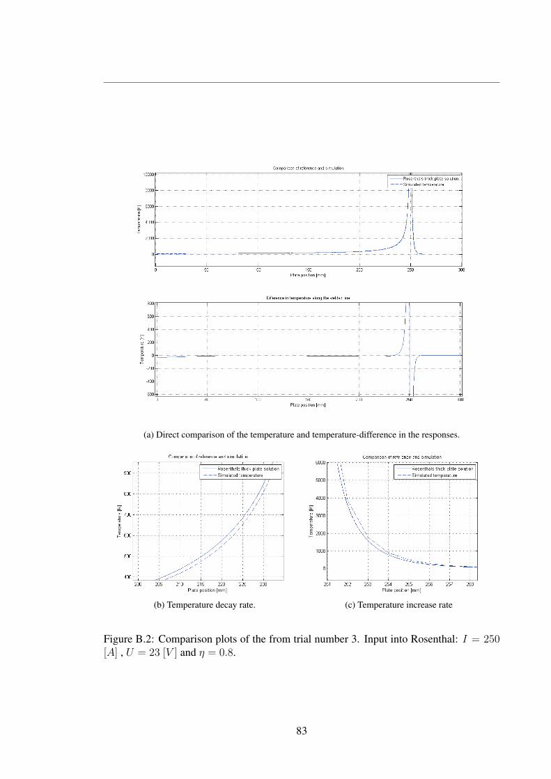
(a) Direct comparison of the temperature and temperature-difference in the responses.
(b) Temperature decay rate. (c) Temperature increase rate
Figure B.2: Comparison plots of the from trial number 3. Input into Rosenthal: I = 250[A] , U = 23 [V ] and η = 0.8.
83
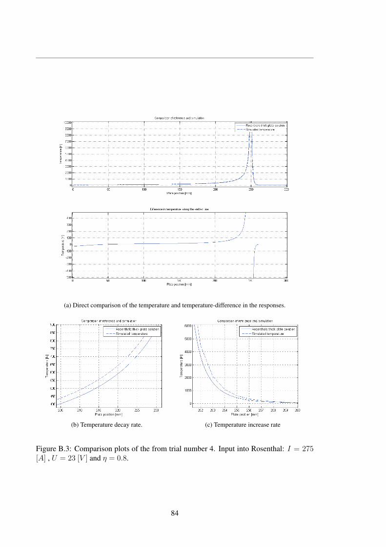
(a) Direct comparison of the temperature and temperature-difference in the responses.
(b) Temperature decay rate. (c) Temperature increase rate
Figure B.3: Comparison plots of the from trial number 4. Input into Rosenthal: I = 275[A] , U = 23 [V ] and η = 0.8.
84

(a) Direct comparison of the temperature and temperature-difference in the responses.
(b) Temperature decay rate. (c) Temperature increase rate
Figure B.4: Comparison plots of the from trial number 5. Input into Rosenthal: I = 320[A] , U = 23 [V ] and η = 0.8.
85

Appendix C
Figures relevant to Chapter 7
87
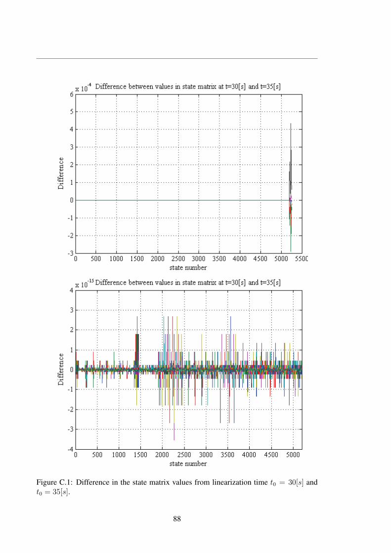
Figure C.1: Difference in the state matrix values from linearization time t0 = 30[s] and
t0 = 35[s].
88

Figure C.2: The state matrix eigenvalues for linearization point t0 = 31[s]
89
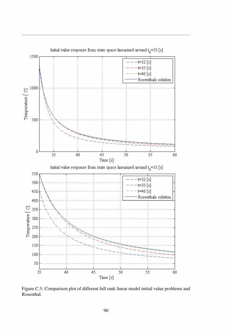
Figure C.3: Comparison plot of different full rank linear model initial value problems and
Rosenthal.
90
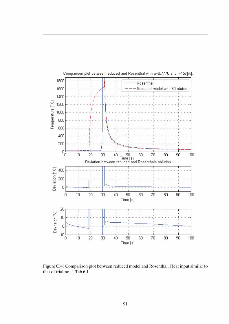
Figure C.4: Comparison plot between reduced model and Rosenthal. Heat input similar to
that of trial no. 1 Tab.6.1
91

Figure C.5: Comparison plot between reduced model and Rosenthal. Heat input similar to
that of trial no. 4 Tab.6.1
92
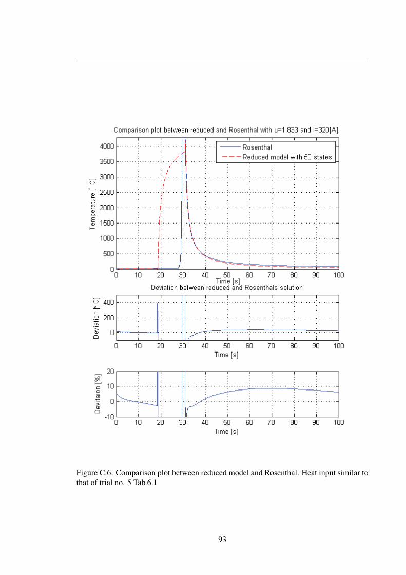
Figure C.6: Comparison plot between reduced model and Rosenthal. Heat input similar to
that of trial no. 5 Tab.6.1
93
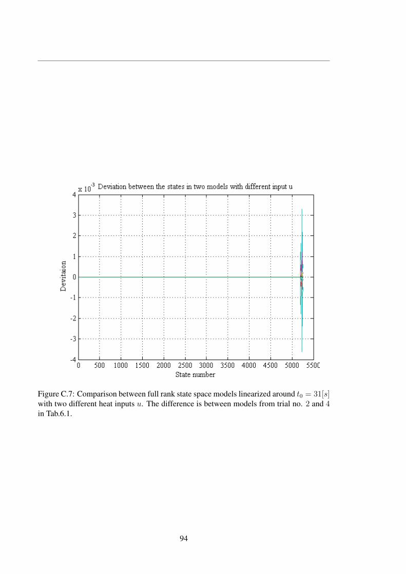
Figure C.7: Comparison between full rank state space models linearized around t0 = 31[s]with two different heat inputs u. The difference is between models from trial no. 2 and 4in Tab.6.1.
94

Appendix D
ThermaCAMTM S65
Figure D.1: The ThermaCAMTM S65 infrared camera
95

IMAGING PERFORMANCE
Field of view/min focus distance 24◦ × 18◦ /0.3 m (with 35 mm lens)
Spatial resolution 1.3 mrad
Accuracy 2◦CThermal sensitivity 0.08◦C at 30◦CFocusing Automatic or manual focus
Electronic zoom function 2x, 4x, 8x interpolating
Digital image enhancement Adaptive digital noise reduction
Built-in digital video 640 × 480 pixels, full color
Detector type Focal Plane Array (FPA),
uncooled micro bolometer
(320 × 240 pixels)
Spectral range 7.5 to 13μm
Image frequency 50/60 Hz, non-interlaced
IMAGE PRESENTATION
Image output RS170 EIA/NTSC or CCIR/PAL
analog composite video
and
FireWire (IEEE-1394) 8/16-bit
digital image output.
MEASUREMENT
Temperature ranges −40◦C up to +1500◦CAccuracy ±2◦C, ±2% of reading
Measurement modes Spot (up to 6), area (4), isotherm, Δ T
Emissivity corrections Variable from 0.1 to 1.0Reflected ambient temperature Automatic, based on input of reflected
temperature correction
External optics / window correction Automatic, based on input of optics/window
transmission and temperature
POWER SOURCE
AC operation AC adapter 110/220 V AC, 50/60 Hz
Voltage 10/30V nominal, < 6W
96

ENVIRONMENTAL SPECIFICATIONS
Operating temperature range −15◦C to +55◦CStorage temperature range −40◦C to +70◦CHumidity Operating and storage 10% to 95%,
non condensing
Encapsulation IP 40 (determined by connector type)
Shock Operational: 25 G, IEC 68-2-29
Vibration Operational: 2 G, IEC 68-2-6
PHYSICAL CHARACTERISTICSWeight, including battery and RC 2.17kg
Size 234mm×124mm×161mm
Tripod mounting Standard 1/4′′ − 20
INTERFACES
Digital image output 6-pin FireWire (IEEE-1394) connector handling
and camera control isochronous. 16-bit digital image data and
asynchronous control data
BNC Composite video (NTSC/PAL)
6-pin screw terminal (upper) Digital I/O: 3 Output- 1 Input
1 Input/Ouput selectable. User configurable*
6-pin screw terminal (lower) Analog I/O: 2 Output - 1 Input,
User configurable*
USER CONFIGURATION TABLE*TYPE FUNCTION REMARK
Digital TTL: Shutter disable, Store image, Isolation and relay function in
input Batch enable external module
Digital TTL Level: Spot / Area threshold alarm, Isolation and relay function
output Internal temperature sensor alarm, V-sync in external module
Analog Spot/Area out 0 − 5 V, Internal Scaled to T-low - T-high
Output temperature sensor alarm, V-sync isolation in external module
Analog External temperature sensor Scaled to T-low - T-high isolation
input in 0 − 10V external module
97


Appendix E
Results from Vicker 10 hardness test
The following tables are the results obtained from the hardness tests performed on the
macros made after the weld-experiments at AKV.
99

Str
ing
no.
89
10
11
12
13
14
1
Dia
g1
Dia
g2
282
277
290
289
285
297
294
290
301
303
306
304
310
308
Aver
age
279.4
289.3
291.0
292.0
302.0
305.0
309.0
Vic
ker
10H
v237.5
221.6
219
217.4
203.3
199.3
194.2
Tri
alno./
Str
ing
no.
89
10
11
12
13
14
2
Dia
g1
Dia
g2
278
272
287
282
300
298
298
307
305
308
310
310
319
322
Aver
age
274.7
289.5
299.0
302.5
306.5
310.0
320.5
Vic
ker
10H
v245.6
229.0
207.4
202.6
197.3
193.0
180.5
Tri
alno./
Str
ing
no.
89
10
11
12
13
14
3
Dia
g1
Dia
g2
278
285
290
282
300
298
293
300
307
303
306
304
312
315
Aver
age
281.5
286.0
299.0
296.5
305.0
305.0
313.5
Vic
ker
10H
v234.0
226.6
207.4
211.0
199.3
199.3
188.6
Tri
alno./
Str
ing
no.
89
10
11
12
13
14
4
Dia
g1
Dia
g2
292
286
288
289
295
286
301
299
310
302
310
312
319
320
Aver
age
288.7
288.5
290.7
300.0
306.0
310.7
319.5
Vic
ker
10H
v222.4
222.7
219.4
206.0
198.0
192.0
181.6
Tri
alno./
Str
ing
no.
89
10
11
12
13
14
5
Dia
g1
Dia
g2
292
290
296
289
300
294
312
306
309
305
305
316
316
313
Aver
age
291.0
292.5
297.0
309.0
307.0
310.5
314.5
Vic
ker
10H
v218.9
216.7
210.2
194.2
196.7
192.3
187.4
Tri
alno./
Str
ing
no.
89
10
11
12
13
14
6
Dia
g1
Dia
g2
286
290
292
297
310
306
304
315
305
304
300
316
320
313
Aver
age
288.0
294.5
308.0
309.5
304.5
308.0
316.5
Vic
ker
10H
v223.5
213.7
195.4
193.5
200.0
195.4
185.0
Table E.1: Hardness results from session 5.
100

Str
ing
no.
89
10
11
12
13
14
1
Dia
g1
Dia
g2
297
299
297
296
305
304
291
300
300
299
304
307
319
318
Aver
age
298.0
296.0
304.0
295.5
299.5
305.5
318.0
Vic
ker
10H
v209.0
212.0
201.0
212.3
206.7
198.6
183.0
Tri
alno./
Str
ing
no.
89
10
11
12
13
14
2
Dia
g1
Dia
g2
283
297
281
285
293
298
295
288
296
299
309
313
317
317
Aver
age
290.0
283.0
295.5
291.5
298.0
311.0
317.0
Vic
ker
10H
v220.5
231.2
212.3
218.2
208.7
191.7
185.0
Tri
alno./
Str
ing
no.
89
10
11
12
13
14
3
Dia
g1
Dia
g2
286
282
284
288
299
299
299
286
287
292
308
307
299
308
Aver
age
283.5
286.0
299.0
292.5
289.4
307.5
303.5
Vic
ker
10H
v230.6
226.6
207.4
216.7
221.3
196.1
201.3
Tri
alno./
Str
ing
no.
89
10
11
12
13
14
4
Dia
g1
Dia
g2
279
281
291
284
304
305
304
307
307
304
303
313
303
306
Aver
age
280.0
287.7
304.5
307.0
305.5
307.5
304.2
Vic
ker
10H
v236.5
224.0
200.0
196.7
198.6
196.0
200.3
Tri
alno./
Str
ing
no.
89
10
11
12
13
14
5
Dia
g1
Dia
g2
297
288
322
311
314
318
302
306
318
317
294
301
329
325
Aver
age
292.5
316.5
316.0
304.0
317.5
297.5
327.0
Vic
ker
10H
v217.0
185.0
185.6
200.6
183.9
209.5
173.4
Tri
alno./
Str
ing
no.
89
10
11
12
13
14
6
Dia
g1
Dia
g2
279
290
288
287
295
295
285
284
284
292
297
297
312
311
Aver
age
284.5
287.5
295.0
284.5
288.0
297.0
311.5
Vic
ker
10H
v229.0
224.3
213.0
229.1
223.5
210.5
191.1
Table E.2: Hardness results from session 7.
101


Appendix F
Sample Welding
103
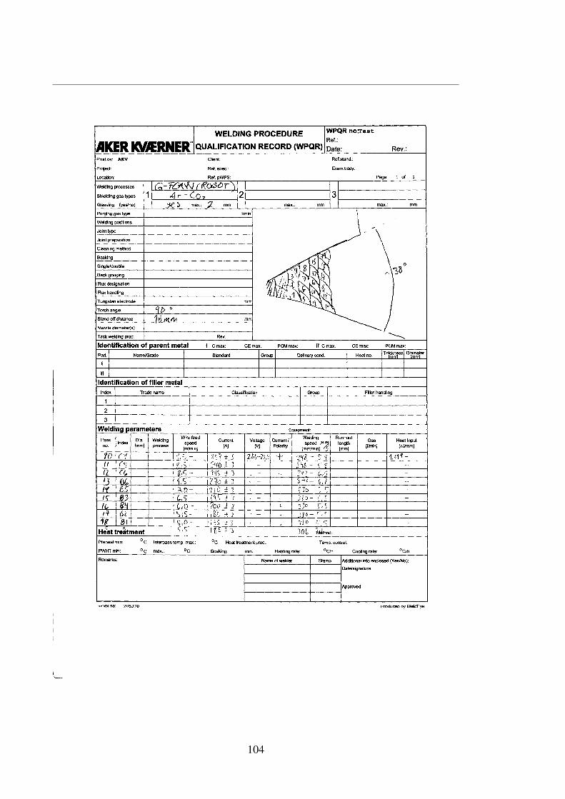
104

Appendix G
Matlab code and FEM-model
The CD contains Matlab files making it possible to recreate the results obtained throughout
the project in addition to the FEM-model used.
105


