
ML-Overview Curve Fitting Decision Theory Probability Theory Kernel Density Estimation Nearest-neighbour Conclusion
Non-parametric MethodsMachine Learning
Alireza Ghane
Non-Parametric Methods Alireza Ghane / Torsten Möller 1

ML-Overview Curve Fitting Decision Theory Probability Theory Kernel Density Estimation Nearest-neighbour Conclusion
Outline
Machine Learning: What, Why, and How?
Curve Fitting: (e.g.) Regression and Model Selection
Decision Theory: ML, Loss Function, MAP
Probability Theory: (e.g.) Probabilities and Parameter Estimation
Kernel Density Estimation
Nearest-neighbour
Conclusion
Non-Parametric Methods Alireza Ghane / Torsten Möller 2

ML-Overview Curve Fitting Decision Theory Probability Theory Kernel Density Estimation Nearest-neighbour Conclusion
Outline
Machine Learning: What, Why, and How?
Curve Fitting: (e.g.) Regression and Model Selection
Decision Theory: ML, Loss Function, MAP
Probability Theory: (e.g.) Probabilities and Parameter Estimation
Kernel Density Estimation
Nearest-neighbour
Conclusion
Non-Parametric Methods Alireza Ghane / Torsten Möller 3

ML-Overview Curve Fitting Decision Theory Probability Theory Kernel Density Estimation Nearest-neighbour Conclusion
Outline
Machine Learning: What, Why, and How?
Curve Fitting: (e.g.) Regression and Model Selection
Decision Theory: ML, Loss Function, MAP
Probability Theory: (e.g.) Probabilities and Parameter Estimation
Kernel Density Estimation
Nearest-neighbour
Conclusion
Non-Parametric Methods Alireza Ghane / Torsten Möller 4
ML-Overview Curve Fitting Decision Theory Probability Theory Kernel Density Estimation Nearest-neighbour Conclusion
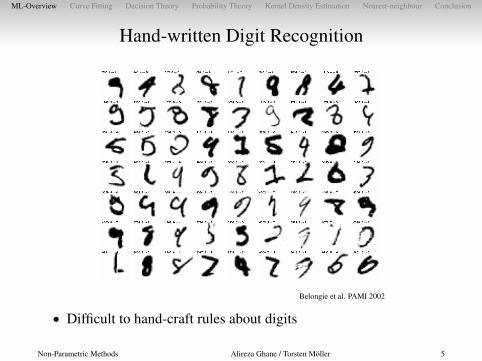
Hand-written Digit Recognition
!"#$%&'"()#*$#+ !,- )( !.,$#/+ +%((/#/01/! 233456 334
7/#()#-! 8/#9 */:: )0 "'%! /$!9 +$"$;$!/ +,/ ") "'/ :$1< )(
8$#%$"%)0 %0 :%&'"%0& =>?@ 2ABC D,!" -$</! %" ($!"/#56E'/ 7#)")"97/ !/:/1"%)0 $:&)#%"'- %! %::,!"#$"/+ %0 F%&6 GH6
C! !//0I 8%/*! $#/ $::)1$"/+ -$%0:9 ()# -)#/ 1)-7:/J1$"/&)#%/! *%"' '%&' *%"'%0 1:$!! 8$#%$;%:%"96 E'/ 1,#8/-$#</+ 3BK7#)") %0 F%&6 L !')*! "'/ %-7#)8/+ 1:$!!%(%1$"%)07/#()#-$01/ ,!%0& "'%! 7#)")"97/ !/:/1"%)0 !"#$"/&9 %0!"/$+)( /.,$::9K!7$1/+ 8%/*!6 M)"/ "'$" */ );"$%0 $ >6? 7/#1/0"
/##)# #$"/ *%"' $0 $8/#$&/ )( )0:9 (),# "*)K+%-/0!%)0$:
8%/*! ()# /$1' "'#//K+%-/0!%)0$: );D/1"I "'$0<! ") "'/
(:/J%;%:%"9 7#)8%+/+ ;9 "'/ -$"1'%0& $:&)#%"'-6
!"# $%&'() *+,-. */0+12.33. 4,3,5,6.
N,# 0/J" /J7/#%-/0" %08):8/! "'/ OAPQKR !'$7/ !%:'),/""/
+$"$;$!/I !7/1%(%1$::9 B)#/ PJ7/#%-/0" BPK3'$7/KG 7$#" SI
*'%1' -/$!,#/! 7/#()#-$01/ )( !%-%:$#%"9K;$!/+ #/"#%/8$:
=>T@6 E'/ +$"$;$!/ 1)0!%!"! )( GI?HH %-$&/!U RH !'$7/
1$"/&)#%/!I >H %-$&/! 7/# 1$"/&)#96 E'/ 7/#()#-$01/ %!
-/$!,#/+ ,!%0& "'/ !)K1$::/+ V;,::!/9/ "/!"IW %0 *'%1' /$1'
!"# $%%% &'()*(+&$,)* ,) -(&&%') ()(./*$* ()0 1(+2$)% $)&%..$3%)+%4 5,.6 784 ),6 784 (-'$. 7997
:;<6 #6 (== >? @AB C;DE=FDD;?;BG 1)$*& @BD@ G;<;@D HD;I< >HJ CB@A>G KLM >H@ >? "94999N6 &AB @BO@ FP>QB BFEA G;<;@ ;IG;EF@BD @AB BOFCR=B IHCPBJ
?>==>SBG PT @AB @JHB =FPB= FIG @AB FDD;<IBG =FPB=6
:;<6 U6 M0 >PVBE@ JBE><I;@;>I HD;I< @AB +,$.W79 GF@F DB@6 +>CRFJ;D>I >?@BD@ DB@ BJJ>J ?>J **04 *AFRB 0;D@FIEB K*0N4 FIG *AFRB 0;D@FIEB S;@A!!"#$%&$' RJ>@>@TRBD K*0WRJ>@>N QBJDHD IHCPBJ >? RJ>@>@TRB Q;BSD6 :>J**0 FIG *04 SB QFJ;BG @AB IHCPBJ >? RJ>@>@TRBD HI;?>JC=T ?>J F==>PVBE@D6 :>J *0WRJ>@>4 @AB IHCPBJ >? RJ>@>@TRBD RBJ >PVBE@ GBRBIGBG >I@AB S;@A;IW>PVBE@ QFJ;F@;>I FD SB== FD @AB PB@SBBIW>PVBE@ D;C;=FJ;@T6
:;<6 "96 -J>@>@TRB Q;BSD DB=BE@BG ?>J @S> G;??BJBI@ M0 >PVBE@D ?J>C @AB+,$. GF@F DB@ HD;I< @AB F=<>J;@AC GBDEJ;PBG ;I *BE@;>I !676 X;@A @A;DFRRJ>FEA4 Q;BSD FJB F==>EF@BG FGFR@;QB=T GBRBIG;I< >I @AB Q;DHF=E>CR=BO;@T >? FI >PVBE@ S;@A JBDRBE@ @> Q;BS;I< FI<=B6
Belongie et al. PAMI 2002
• Difficult to hand-craft rules about digits
Non-Parametric Methods Alireza Ghane / Torsten Möller 5
ML-Overview Curve Fitting Decision Theory Probability Theory Kernel Density Estimation Nearest-neighbour Conclusion
Hand-written Digit Recognition
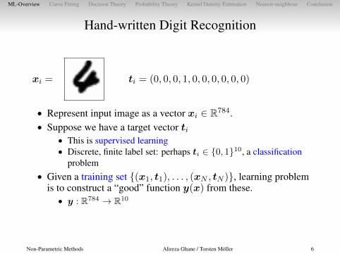
xi =
!"#$%&'"()#*$#+ !,- )( !.,$#/+ +%((/#/01/! 233456 334
7/#()#-! 8/#9 */:: )0 "'%! /$!9 +$"$;$!/ +,/ ") "'/ :$1< )(
8$#%$"%)0 %0 :%&'"%0& =>?@ 2ABC D,!" -$</! %" ($!"/#56E'/ 7#)")"97/ !/:/1"%)0 $:&)#%"'- %! %::,!"#$"/+ %0 F%&6 GH6
C! !//0I 8%/*! $#/ $::)1$"/+ -$%0:9 ()# -)#/ 1)-7:/J1$"/&)#%/! *%"' '%&' *%"'%0 1:$!! 8$#%$;%:%"96 E'/ 1,#8/-$#</+ 3BK7#)") %0 F%&6 L !')*! "'/ %-7#)8/+ 1:$!!%(%1$"%)07/#()#-$01/ ,!%0& "'%! 7#)")"97/ !/:/1"%)0 !"#$"/&9 %0!"/$+)( /.,$::9K!7$1/+ 8%/*!6 M)"/ "'$" */ );"$%0 $ >6? 7/#1/0"
/##)# #$"/ *%"' $0 $8/#$&/ )( )0:9 (),# "*)K+%-/0!%)0$:
8%/*! ()# /$1' "'#//K+%-/0!%)0$: );D/1"I "'$0<! ") "'/
(:/J%;%:%"9 7#)8%+/+ ;9 "'/ -$"1'%0& $:&)#%"'-6
!"# $%&'() *+,-. */0+12.33. 4,3,5,6.
N,# 0/J" /J7/#%-/0" %08):8/! "'/ OAPQKR !'$7/ !%:'),/""/
+$"$;$!/I !7/1%(%1$::9 B)#/ PJ7/#%-/0" BPK3'$7/KG 7$#" SI
*'%1' -/$!,#/! 7/#()#-$01/ )( !%-%:$#%"9K;$!/+ #/"#%/8$:
=>T@6 E'/ +$"$;$!/ 1)0!%!"! )( GI?HH %-$&/!U RH !'$7/
1$"/&)#%/!I >H %-$&/! 7/# 1$"/&)#96 E'/ 7/#()#-$01/ %!
-/$!,#/+ ,!%0& "'/ !)K1$::/+ V;,::!/9/ "/!"IW %0 *'%1' /$1'
!"# $%%% &'()*(+&$,)* ,) -(&&%') ()(./*$* ()0 1(+2$)% $)&%..$3%)+%4 5,.6 784 ),6 784 (-'$. 7997
:;<6 #6 (== >? @AB C;DE=FDD;?;BG 1)$*& @BD@ G;<;@D HD;I< >HJ CB@A>G KLM >H@ >? "94999N6 &AB @BO@ FP>QB BFEA G;<;@ ;IG;EF@BD @AB BOFCR=B IHCPBJ
?>==>SBG PT @AB @JHB =FPB= FIG @AB FDD;<IBG =FPB=6
:;<6 U6 M0 >PVBE@ JBE><I;@;>I HD;I< @AB +,$.W79 GF@F DB@6 +>CRFJ;D>I >?@BD@ DB@ BJJ>J ?>J **04 *AFRB 0;D@FIEB K*0N4 FIG *AFRB 0;D@FIEB S;@A!!"#$%&$' RJ>@>@TRBD K*0WRJ>@>N QBJDHD IHCPBJ >? RJ>@>@TRB Q;BSD6 :>J**0 FIG *04 SB QFJ;BG @AB IHCPBJ >? RJ>@>@TRBD HI;?>JC=T ?>J F==>PVBE@D6 :>J *0WRJ>@>4 @AB IHCPBJ >? RJ>@>@TRBD RBJ >PVBE@ GBRBIGBG >I@AB S;@A;IW>PVBE@ QFJ;F@;>I FD SB== FD @AB PB@SBBIW>PVBE@ D;C;=FJ;@T6
:;<6 "96 -J>@>@TRB Q;BSD DB=BE@BG ?>J @S> G;??BJBI@ M0 >PVBE@D ?J>C @AB+,$. GF@F DB@ HD;I< @AB F=<>J;@AC GBDEJ;PBG ;I *BE@;>I !676 X;@A @A;DFRRJ>FEA4 Q;BSD FJB F==>EF@BG FGFR@;QB=T GBRBIG;I< >I @AB Q;DHF=E>CR=BO;@T >? FI >PVBE@ S;@A JBDRBE@ @> Q;BS;I< FI<=B6
ti = (0, 0, 0, 1, 0, 0, 0, 0, 0, 0)
• Represent input image as a vector xi ∈ R784.• Suppose we have a target vector ti
• This is supervised learning• Discrete, finite label set: perhaps ti ∈ {0, 1}10, a classification
problem• Given a training set {(x1, t1), . . . , (xN , tN )}, learning problem
is to construct a “good” function y(x) from these.• y : R784 → R10
Non-Parametric Methods Alireza Ghane / Torsten Möller 6

ML-Overview Curve Fitting Decision Theory Probability Theory Kernel Density Estimation Nearest-neighbour Conclusion
Face Detection
Schneiderman and Kanade, IJCV 2002
• Classification problem• ti ∈ {0, 1, 2}, non-face, frontal face, profile face.
Non-Parametric Methods Alireza Ghane / Torsten Möller 7

ML-Overview Curve Fitting Decision Theory Probability Theory Kernel Density Estimation Nearest-neighbour Conclusion
Spam Detection
• Classification problem• ti ∈ {0, 1}, non-spam, spam• xi counts of words, e.g. Viagra, stock, outperform,multi-bagger
Non-Parametric Methods Alireza Ghane / Torsten Möller 8
ML-Overview Curve Fitting Decision Theory Probability Theory Kernel Density Estimation Nearest-neighbour Conclusion
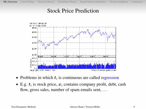
Stock Price Prediction
• Problems in which ti is continuous are called regression• E.g. ti is stock price, xi contains company profit, debt, cash
flow, gross sales, number of spam emails sent, . . .
Non-Parametric Methods Alireza Ghane / Torsten Möller 9

ML-Overview Curve Fitting Decision Theory Probability Theory Kernel Density Estimation Nearest-neighbour Conclusion
Clustering Images
Wang et al., CVPR 2006
• Only xi is defined: unsupervised learning• E.g. xi describes image, find groups of similar images
Non-Parametric Methods Alireza Ghane / Torsten Möller 10

ML-Overview Curve Fitting Decision Theory Probability Theory Kernel Density Estimation Nearest-neighbour Conclusion
Types of Learning Problems
• Supervised Learning• Classification• Regression
• Unsupervised Learning• Density estimation• Clustering: k-means, mixture models, hierarchical clustering• Hidden Markov models
• Reinforcement Learning
Non-Parametric Methods Alireza Ghane / Torsten Möller 11

ML-Overview Curve Fitting Decision Theory Probability Theory Kernel Density Estimation Nearest-neighbour Conclusion
Outline
Machine Learning: What, Why, and How?
Curve Fitting: (e.g.) Regression and Model Selection
Decision Theory: ML, Loss Function, MAP
Probability Theory: (e.g.) Probabilities and Parameter Estimation
Kernel Density Estimation
Nearest-neighbour
Conclusion
Non-Parametric Methods Alireza Ghane / Torsten Möller 12
ML-Overview Curve Fitting Decision Theory Probability Theory Kernel Density Estimation Nearest-neighbour Conclusion
Outline
Machine Learning: What, Why, and How?
Curve Fitting: (e.g.) Regression and Model Selection
Decision Theory: ML, Loss Function, MAP
Probability Theory: (e.g.) Probabilities and Parameter Estimation
Kernel Density Estimation
Nearest-neighbour
Conclusion
Non-Parametric Methods Alireza Ghane / Torsten Möller 13
ML-Overview Curve Fitting Decision Theory Probability Theory Kernel Density Estimation Nearest-neighbour Conclusion
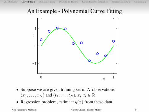
An Example - Polynomial Curve Fitting
�
�
0 1
−1
0
1
• Suppose we are given training set of N observations(x1, . . . , xN ) and (t1, . . . , tN ), xi, ti ∈ R
• Regression problem, estimate y(x) from these data
Non-Parametric Methods Alireza Ghane / Torsten Möller 14

ML-Overview Curve Fitting Decision Theory Probability Theory Kernel Density Estimation Nearest-neighbour Conclusion
Polynomial Curve Fitting
• What form is y(x)?• Let’s try polynomials of degree M :
y(x,w) = w0+w1x+w2x2+. . .+wMx
M
• This is the hypothesis space.
• How do we measure success?• Sum of squared errors:
E(w) =1
2
N∑n=1
{y(xn,w)− tn}2
• Among functions in the class, choose thatwhich minimizes this error
�
�
0 1
−1
0
1
t
x
y(xn,w)
tn
xn
Non-Parametric Methods Alireza Ghane / Torsten Möller 15

ML-Overview Curve Fitting Decision Theory Probability Theory Kernel Density Estimation Nearest-neighbour Conclusion
Which Degree of Polynomial?
�
�
�����
0 1
−1
0
1
�
�
�����
0 1
−1
0
1
�
�
�����
0 1
−1
0
1
�
�
�����
0 1
−1
0
1
• A model selection problem• M = 9→ E(w∗) = 0: This is over-fitting
Non-Parametric Methods Alireza Ghane / Torsten Möller 16

ML-Overview Curve Fitting Decision Theory Probability Theory Kernel Density Estimation Nearest-neighbour Conclusion
Generalization
�
�����
0 3 6 90
0.5
1TrainingTest
• Generalization is the holy grail of ML• Want good performance for new data
• Measure generalization using a separate set• Use root-mean-squared (RMS) error: ERMS =
√2E(w∗)/N
Non-Parametric Methods Alireza Ghane / Torsten Möller 17
ML-Overview Curve Fitting Decision Theory Probability Theory Kernel Density Estimation Nearest-neighbour Conclusion
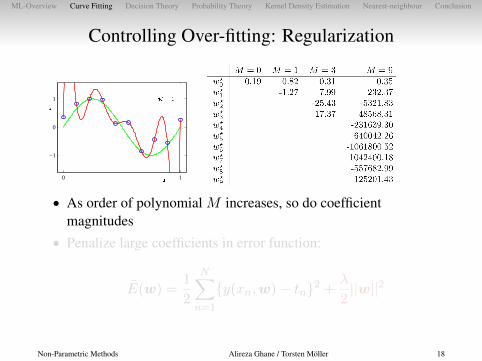
Controlling Over-fitting: Regularization
�
�
�����
0 1
−1
0
1
• As order of polynomial M increases, so do coefficientmagnitudes
• Penalize large coefficients in error function:
E(w) =1
2
N∑n=1
{y(xn,w)− tn}2 +λ
2||w||2
Non-Parametric Methods Alireza Ghane / Torsten Möller 18
ML-Overview Curve Fitting Decision Theory Probability Theory Kernel Density Estimation Nearest-neighbour Conclusion
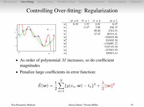
Controlling Over-fitting: Regularization
�
�
�����
0 1
−1
0
1
• As order of polynomial M increases, so do coefficientmagnitudes
• Penalize large coefficients in error function:
E(w) =1
2
N∑n=1
{y(xn,w)− tn}2 +λ
2||w||2
Non-Parametric Methods Alireza Ghane / Torsten Möller 19
ML-Overview Curve Fitting Decision Theory Probability Theory Kernel Density Estimation Nearest-neighbour Conclusion
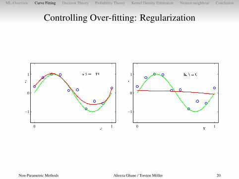
Controlling Over-fitting: Regularization
�
�
� ������� �
0 1
−1
0
1
�
�
� ������
0 1
−1
0
1
Non-Parametric Methods Alireza Ghane / Torsten Möller 20

ML-Overview Curve Fitting Decision Theory Probability Theory Kernel Density Estimation Nearest-neighbour Conclusion
Controlling Over-fitting: Regularization
�����
� ���−35 −30 −25 −200
0.5
1TrainingTest
• Note the ERMS for the training set. Perfect match of training setwith the model is a result of over-fitting
• Training and test error show similar trend
Non-Parametric Methods Alireza Ghane / Torsten Möller 21

ML-Overview Curve Fitting Decision Theory Probability Theory Kernel Density Estimation Nearest-neighbour Conclusion
Over-fitting: Dataset size
�
�
�������
0 1
−1
0
1
�
�
���������
0 1
−1
0
1
• With more data, more complex model (M = 9) can be fit• Rule of thumb: 10 datapoints for each parameter
Non-Parametric Methods Alireza Ghane / Torsten Möller 22

ML-Overview Curve Fitting Decision Theory Probability Theory Kernel Density Estimation Nearest-neighbour Conclusion
Validation Set
• Split training data into training set and validation set• Train different models (e.g. diff. order polynomials) on training
set• Choose model (e.g. order of polynomial) with minimum error on
validation set
Non-Parametric Methods Alireza Ghane / Torsten Möller 23

ML-Overview Curve Fitting Decision Theory Probability Theory Kernel Density Estimation Nearest-neighbour Conclusion
Cross-validation
run 1
run 2
run 3
run 4
• Data are often limited• Cross-validation creates S groups of data, use S − 1 to train,
other to validate• Extreme case leave-one-out cross-validation (LOO-CV): S is
number of training data points• Cross-validation is an effective method for model selection, but
can be slow• Models with multiple complexity parameters: exponential
number of runs
Non-Parametric Methods Alireza Ghane / Torsten Möller 24

ML-Overview Curve Fitting Decision Theory Probability Theory Kernel Density Estimation Nearest-neighbour Conclusion
Summary
• Want models that generalize to new data• Train model on training set• Measure performance on held-out test set
• Performance on test set is good estimate of performance on newdata
Non-Parametric Methods Alireza Ghane / Torsten Möller 25
ML-Overview Curve Fitting Decision Theory Probability Theory Kernel Density Estimation Nearest-neighbour Conclusion
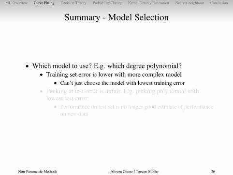
Summary - Model Selection
• Which model to use? E.g. which degree polynomial?• Training set error is lower with more complex model
• Can’t just choose the model with lowest training error• Peeking at test error is unfair. E.g. picking polynomial with
lowest test error• Performance on test set is no longer good estimate of performance
on new data
Non-Parametric Methods Alireza Ghane / Torsten Möller 26

ML-Overview Curve Fitting Decision Theory Probability Theory Kernel Density Estimation Nearest-neighbour Conclusion
Summary - Model Selection
• Which model to use? E.g. which degree polynomial?• Training set error is lower with more complex model
• Can’t just choose the model with lowest training error• Peeking at test error is unfair. E.g. picking polynomial with
lowest test error• Performance on test set is no longer good estimate of performance
on new data
Non-Parametric Methods Alireza Ghane / Torsten Möller 27

ML-Overview Curve Fitting Decision Theory Probability Theory Kernel Density Estimation Nearest-neighbour Conclusion
Summary - Solutions I
• Use a validation set• Train models on training set. E.g. different degree polynomials• Measure performance on held-out validation set• Measure performance of that model on held-out test set
• Can use cross-validation on training set instead of a separatevalidation set if little data and lots of time
• Choose model with lowest error over all cross-validation folds(e.g. polynomial degree)
• Retrain that model using all training data (e.g. polynomialcoefficients)
Non-Parametric Methods Alireza Ghane / Torsten Möller 28
ML-Overview Curve Fitting Decision Theory Probability Theory Kernel Density Estimation Nearest-neighbour Conclusion
Summary - Solutions I
• Use a validation set• Train models on training set. E.g. different degree polynomials• Measure performance on held-out validation set• Measure performance of that model on held-out test set
• Can use cross-validation on training set instead of a separatevalidation set if little data and lots of time
• Choose model with lowest error over all cross-validation folds(e.g. polynomial degree)
• Retrain that model using all training data (e.g. polynomialcoefficients)
Non-Parametric Methods Alireza Ghane / Torsten Möller 29

ML-Overview Curve Fitting Decision Theory Probability Theory Kernel Density Estimation Nearest-neighbour Conclusion
Summary - Solutions II
• Use regularization• Train complex model (e.g high order polynomial) but penalize
being “too complex” (e.g. large weight magnitudes)• Need to balance error vs. regularization (λ)
• Choose λ using cross-validation
• Get more data
Non-Parametric Methods Alireza Ghane / Torsten Möller 30

ML-Overview Curve Fitting Decision Theory Probability Theory Kernel Density Estimation Nearest-neighbour Conclusion
Summary - Solutions II
• Use regularization• Train complex model (e.g high order polynomial) but penalize
being “too complex” (e.g. large weight magnitudes)• Need to balance error vs. regularization (λ)
• Choose λ using cross-validation
• Get more data
Non-Parametric Methods Alireza Ghane / Torsten Möller 31
ML-Overview Curve Fitting Decision Theory Probability Theory Kernel Density Estimation Nearest-neighbour Conclusion
Outline
Machine Learning: What, Why, and How?
Curve Fitting: (e.g.) Regression and Model Selection
Decision Theory: ML, Loss Function, MAP
Probability Theory: (e.g.) Probabilities and Parameter Estimation
Kernel Density Estimation
Nearest-neighbour
Conclusion
Non-Parametric Methods Alireza Ghane / Torsten Möller 32

Outline
Machine Learning: What, Why, and How?
Curve Fitting: (e.g.) Regression and Model Selection
Decision Theory: ML, Loss Function, MAP
Probability Theory: (e.g.) Probabilities and Parameter Estimation
Kernel Density Estimation
Nearest-neighbour
Conclusion

ML-Overview Curve Fitting Decision Theory Probability Theory Kernel Density Estimation Nearest-neighbour Conclusion
Decision Theory
For a sample x, decide which class(Ck) it is from.
Ideas:• Maximum Likelihood• Minimum Loss/Cost (e.g. misclassification rate)• Maximum Aposteriori (MAP)
Intro. to Machine Learning Alireza Ghane 34
ML-Overview Curve Fitting Decision Theory Probability Theory Kernel Density Estimation Nearest-neighbour Conclusion
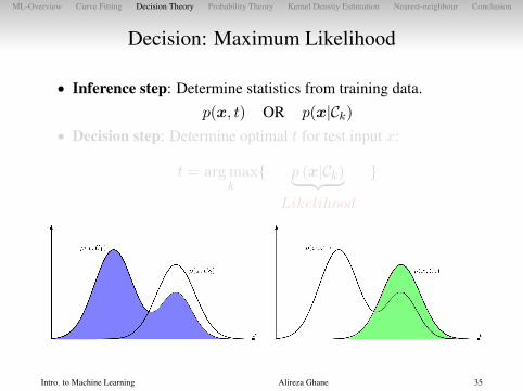
Decision: Maximum Likelihood
• Inference step: Determine statistics from training data.
p(x, t) OR p(x|Ck)• Decision step: Determine optimal t for test input x:
t = arg maxk{ p (x|Ck)︸ ︷︷ ︸ }
Likelihood
Intro. to Machine Learning Alireza Ghane 35

ML-Overview Curve Fitting Decision Theory Probability Theory Kernel Density Estimation Nearest-neighbour Conclusion
Decision: Maximum Likelihood
• Inference step: Determine statistics from training data.
p(x, t) OR p(x|Ck)• Decision step: Determine optimal t for test input x:
t = arg maxk{ p (x|Ck)︸ ︷︷ ︸ }
Likelihood
Intro. to Machine Learning Alireza Ghane 36

ML-Overview Curve Fitting Decision Theory Probability Theory Kernel Density Estimation Nearest-neighbour Conclusion
Decision: Maximum Likelihood
• Inference step: Determine statistics from training data.
p(x, t) OR p(x|Ck)• Decision step: Determine optimal t for test input x:
t = arg maxk{ p (x|Ck)︸ ︷︷ ︸ }
Likelihood
Intro. to Machine Learning Alireza Ghane 37

ML-Overview Curve Fitting Decision Theory Probability Theory Kernel Density Estimation Nearest-neighbour Conclusion
Decision: Minimum Misclassification Rate
q(mistake) = p (x ∈ R1, C2) + p (x ∈ R2, C1)=
∫R1p (x, C2) dx +
∫R2p (x, C1) dx
q(mistake) =∑k
∑j
∫Rjp (x, Ck) dx
R1 R2
x0 x
p(x, C1)
p(x, C2)
x
x: decision boundary.x0: optimal decision boundary
x0 : arg minR1
{p (mistake)}
Intro. to Machine Learning Alireza Ghane 38

ML-Overview Curve Fitting Decision Theory Probability Theory Kernel Density Estimation Nearest-neighbour Conclusion
Decision: Minimum Misclassification Rate
q(mistake) = p (x ∈ R1, C2) + p (x ∈ R2, C1)=
∫R1p (x, C2) dx +
∫R2p (x, C1) dx
q(mistake) =∑k
∑j
∫Rjp (x, Ck) dx
R1 R2
x0 x
p(x, C1)
p(x, C2)
x
x: decision boundary.x0: optimal decision boundary
x0 : arg minR1
{p (mistake)}
Intro. to Machine Learning Alireza Ghane 39

ML-Overview Curve Fitting Decision Theory Probability Theory Kernel Density Estimation Nearest-neighbour Conclusion
Decision: Minimum Loss/Cost
• Misclassification rate:
R : arg min{Ri|i∈{1,··· ,K}}
∑k
∑j
L (Rj , Ck)
• Weighted loss/cost function:
R : arg min{Ri|i∈{1,··· ,K}}
∑k
∑j
Wj,kL (Rj , Ck)
Is useful when:
• The population of the classes are different• The failure cost is non-symmetric• · · ·
Intro. to Machine Learning Alireza Ghane 40

ML-Overview Curve Fitting Decision Theory Probability Theory Kernel Density Estimation Nearest-neighbour Conclusion
Decision: Maximum Aposteriori (MAP)
Bayes’ Theorem: P{A|B} = P{B|A}P{A}P{B}
p(Ck|x)︸ ︷︷ ︸Posterior
∝ p(x|Ck)︸ ︷︷ ︸Likelihood
p(Ck)︸ ︷︷ ︸Prior
• Provides an Aposteriori Belief for the estimation, rather than asingle point estimate.
• Can utilize Apriori Information in the decision.
Intro. to Machine Learning Alireza Ghane 41

ML-Overview Curve Fitting Decision Theory Probability Theory Kernel Density Estimation Nearest-neighbour Conclusion
Outline
Machine Learning: What, Why, and How?
Curve Fitting: (e.g.) Regression and Model Selection
Decision Theory: ML, Loss Function, MAP
Probability Theory: (e.g.) Probabilities and Parameter Estimation
Kernel Density Estimation
Nearest-neighbour
Conclusion
Non-Parametric Methods Alireza Ghane / Torsten Möller 42

Outline
Machine Learning: What, Why, and How?
Curve Fitting: (e.g.) Regression and Model Selection
Decision Theory: ML, Loss Function, MAP
Probability Theory: (e.g.) Probabilities and Parameter Estimation
Kernel Density Estimation
Nearest-neighbour
Conclusion

ML-Overview Curve Fitting Decision Theory Probability Theory Kernel Density Estimation Nearest-neighbour Conclusion
Coin Tossing
• Let’s say you’re given a coin, and you want to find outP (heads), the probability that if you flip it it lands as “heads”.
• Flip it a few times: H H T
• P (heads) = 2/3
• Hmm... is this rigorous? Does this make sense?
Non-Parametric Methods Alireza Ghane / Torsten Möller 44

ML-Overview Curve Fitting Decision Theory Probability Theory Kernel Density Estimation Nearest-neighbour Conclusion
Coin Tossing
• Let’s say you’re given a coin, and you want to find outP (heads), the probability that if you flip it it lands as “heads”.
• Flip it a few times: H H T
• P (heads) = 2/3
• Hmm... is this rigorous? Does this make sense?
Non-Parametric Methods Alireza Ghane / Torsten Möller 45

ML-Overview Curve Fitting Decision Theory Probability Theory Kernel Density Estimation Nearest-neighbour Conclusion
Coin Tossing
• Let’s say you’re given a coin, and you want to find outP (heads), the probability that if you flip it it lands as “heads”.
• Flip it a few times: H H T
• P (heads) = 2/3
• Hmm... is this rigorous? Does this make sense?
Non-Parametric Methods Alireza Ghane / Torsten Möller 46

ML-Overview Curve Fitting Decision Theory Probability Theory Kernel Density Estimation Nearest-neighbour Conclusion
Coin Tossing - Model
• Bernoulli distribution P (heads) = µ, P (tails) = 1− µ• Assume coin flips are independent and identically distributed
(i.i.d.)• i.e. All are separate samples from the Bernoulli distribution
• Given data D = {x1, . . . , xN}, heads: xi = 1, tails: xi = 0, thelikelihood of the data is:
p(D|µ) =
N∏n=1
p(xn|µ) =
N∏n=1
µxn(1− µ)1−xn
Non-Parametric Methods Alireza Ghane / Torsten Möller 47
ML-Overview Curve Fitting Decision Theory Probability Theory Kernel Density Estimation Nearest-neighbour Conclusion
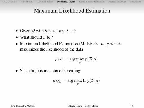
Maximum Likelihood Estimation
• Given D with h heads and t tails• What should µ be?• Maximum Likelihood Estimation (MLE): choose µ which
maximizes the likelihood of the data
µML = arg maxµ
p(D|µ)
• Since ln(·) is monotone increasing:
µML = arg maxµ
ln p(D|µ)
Non-Parametric Methods Alireza Ghane / Torsten Möller 48

ML-Overview Curve Fitting Decision Theory Probability Theory Kernel Density Estimation Nearest-neighbour Conclusion
Maximum Likelihood Estimation• Likelihood:
p(D|µ) =
N∏n=1
µxn(1− µ)1−xn
• Log-likelihood:
ln p(D|µ) =
N∑n=1
xn lnµ+ (1− xn) ln(1− µ)
• Take derivative, set to 0:
d
dµln p(D|µ) =
N∑n=1
xn1
µ− (1− xn)
1
1− µ=
1
µh− 1
1− µt
⇒ µ =h
t+ hNon-Parametric Methods Alireza Ghane / Torsten Möller 49

ML-Overview Curve Fitting Decision Theory Probability Theory Kernel Density Estimation Nearest-neighbour Conclusion
Maximum Likelihood Estimation• Likelihood:
p(D|µ) =
N∏n=1
µxn(1− µ)1−xn
• Log-likelihood:
ln p(D|µ) =
N∑n=1
xn lnµ+ (1− xn) ln(1− µ)
• Take derivative, set to 0:
d
dµln p(D|µ) =
N∑n=1
xn1
µ− (1− xn)
1
1− µ=
1
µh− 1
1− µt
⇒ µ =h
t+ hNon-Parametric Methods Alireza Ghane / Torsten Möller 50

ML-Overview Curve Fitting Decision Theory Probability Theory Kernel Density Estimation Nearest-neighbour Conclusion
Maximum Likelihood Estimation• Likelihood:
p(D|µ) =
N∏n=1
µxn(1− µ)1−xn
• Log-likelihood:
ln p(D|µ) =
N∑n=1
xn lnµ+ (1− xn) ln(1− µ)
• Take derivative, set to 0:
d
dµln p(D|µ) =
N∑n=1
xn1
µ− (1− xn)
1
1− µ=
1
µh− 1
1− µt
⇒ µ =h
t+ hNon-Parametric Methods Alireza Ghane / Torsten Möller 51

ML-Overview Curve Fitting Decision Theory Probability Theory Kernel Density Estimation Nearest-neighbour Conclusion
Maximum Likelihood Estimation• Likelihood:
p(D|µ) =
N∏n=1
µxn(1− µ)1−xn
• Log-likelihood:
ln p(D|µ) =
N∑n=1
xn lnµ+ (1− xn) ln(1− µ)
• Take derivative, set to 0:
d
dµln p(D|µ) =
N∑n=1
xn1
µ− (1− xn)
1
1− µ=
1
µh− 1
1− µt
⇒ µ =h
t+ hNon-Parametric Methods Alireza Ghane / Torsten Möller 52

ML-Overview Curve Fitting Decision Theory Probability Theory Kernel Density Estimation Nearest-neighbour Conclusion
Maximum Likelihood Estimation• Likelihood:
p(D|µ) =
N∏n=1
µxn(1− µ)1−xn
• Log-likelihood:
ln p(D|µ) =
N∑n=1
xn lnµ+ (1− xn) ln(1− µ)
• Take derivative, set to 0:
d
dµln p(D|µ) =
N∑n=1
xn1
µ− (1− xn)
1
1− µ=
1
µh− 1
1− µt
⇒ µ =h
t+ hNon-Parametric Methods Alireza Ghane / Torsten Möller 53

ML-Overview Curve Fitting Decision Theory Probability Theory Kernel Density Estimation Nearest-neighbour Conclusion
Bayesian Learning
• Wait, does this make sense? What if I flip 1 time, heads? Do Ibelieve µ=1?
• Learn µ the Bayesian way:
P (µ|D) =P (D|µ)P (µ)
P (D)
P (µ|D)︸ ︷︷ ︸posterior
∝ P (D|µ)︸ ︷︷ ︸likelihood
P (µ)︸ ︷︷ ︸prior
• Prior encodes knowledge that most coins are 50-50• Conjugate prior makes math simpler, easy interpretation
• For Bernoulli, the beta distribution is its conjugate
Non-Parametric Methods Alireza Ghane / Torsten Möller 54

ML-Overview Curve Fitting Decision Theory Probability Theory Kernel Density Estimation Nearest-neighbour Conclusion
Bayesian Learning
• Wait, does this make sense? What if I flip 1 time, heads? Do Ibelieve µ=1?
• Learn µ the Bayesian way:
P (µ|D) =P (D|µ)P (µ)
P (D)
P (µ|D)︸ ︷︷ ︸posterior
∝ P (D|µ)︸ ︷︷ ︸likelihood
P (µ)︸ ︷︷ ︸prior
• Prior encodes knowledge that most coins are 50-50• Conjugate prior makes math simpler, easy interpretation
• For Bernoulli, the beta distribution is its conjugate
Non-Parametric Methods Alireza Ghane / Torsten Möller 55

ML-Overview Curve Fitting Decision Theory Probability Theory Kernel Density Estimation Nearest-neighbour Conclusion
Bayesian Learning
• Wait, does this make sense? What if I flip 1 time, heads? Do Ibelieve µ=1?
• Learn µ the Bayesian way:
P (µ|D) =P (D|µ)P (µ)
P (D)
P (µ|D)︸ ︷︷ ︸posterior
∝ P (D|µ)︸ ︷︷ ︸likelihood
P (µ)︸ ︷︷ ︸prior
• Prior encodes knowledge that most coins are 50-50• Conjugate prior makes math simpler, easy interpretation
• For Bernoulli, the beta distribution is its conjugate
Non-Parametric Methods Alireza Ghane / Torsten Möller 56

ML-Overview Curve Fitting Decision Theory Probability Theory Kernel Density Estimation Nearest-neighbour Conclusion
Beta Distribution• We will use the Beta distribution to express our prior knowledge
about coins:
Beta(µ|a, b) =Γ(a+ b)
Γ(a)Γ(b)︸ ︷︷ ︸normalization
µa−1(1− µ)b−1
• Parameters a and b control the shape of this distribution
Non-Parametric Methods Alireza Ghane / Torsten Möller 57

ML-Overview Curve Fitting Decision Theory Probability Theory Kernel Density Estimation Nearest-neighbour Conclusion
Posterior
P (µ|D) ∝ P (D|µ)P (µ)
∝N∏n=1
µxn(1− µ)1−xn
︸ ︷︷ ︸likelihood
µa−1(1− µ)b−1︸ ︷︷ ︸prior
∝ µh(1− µ)tµa−1(1− µ)b−1
∝ µh+a−1(1− µ)t+b−1
• Simple form for posterior is due to use of conjugate prior• Parameters a and b act as extra observations• Note that as N = h+ t→∞, prior is ignored
Non-Parametric Methods Alireza Ghane / Torsten Möller 58

ML-Overview Curve Fitting Decision Theory Probability Theory Kernel Density Estimation Nearest-neighbour Conclusion
Posterior
P (µ|D) ∝ P (D|µ)P (µ)
∝N∏n=1
µxn(1− µ)1−xn
︸ ︷︷ ︸likelihood
µa−1(1− µ)b−1︸ ︷︷ ︸prior
∝ µh(1− µ)tµa−1(1− µ)b−1
∝ µh+a−1(1− µ)t+b−1
• Simple form for posterior is due to use of conjugate prior• Parameters a and b act as extra observations• Note that as N = h+ t→∞, prior is ignored
Non-Parametric Methods Alireza Ghane / Torsten Möller 59

ML-Overview Curve Fitting Decision Theory Probability Theory Kernel Density Estimation Nearest-neighbour Conclusion
Posterior
P (µ|D) ∝ P (D|µ)P (µ)
∝N∏n=1
µxn(1− µ)1−xn
︸ ︷︷ ︸likelihood
µa−1(1− µ)b−1︸ ︷︷ ︸prior
∝ µh(1− µ)tµa−1(1− µ)b−1
∝ µh+a−1(1− µ)t+b−1
• Simple form for posterior is due to use of conjugate prior• Parameters a and b act as extra observations• Note that as N = h+ t→∞, prior is ignored
Non-Parametric Methods Alireza Ghane / Torsten Möller 60

ML-Overview Curve Fitting Decision Theory Probability Theory Kernel Density Estimation Nearest-neighbour Conclusion
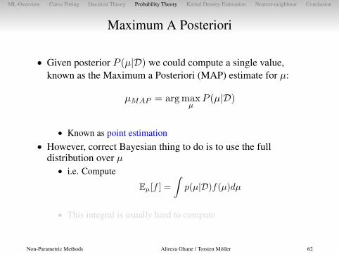
Maximum A Posteriori
• Given posterior P (µ|D) we could compute a single value,known as the Maximum a Posteriori (MAP) estimate for µ:
µMAP = arg maxµ
P (µ|D)
• Known as point estimation• However, correct Bayesian thing to do is to use the full
distribution over µ• i.e. Compute
Eµ[f ] =
∫p(µ|D)f(µ)dµ
• This integral is usually hard to compute
Non-Parametric Methods Alireza Ghane / Torsten Möller 61
ML-Overview Curve Fitting Decision Theory Probability Theory Kernel Density Estimation Nearest-neighbour Conclusion
Maximum A Posteriori
• Given posterior P (µ|D) we could compute a single value,known as the Maximum a Posteriori (MAP) estimate for µ:
µMAP = arg maxµ
P (µ|D)
• Known as point estimation• However, correct Bayesian thing to do is to use the full
distribution over µ• i.e. Compute
Eµ[f ] =
∫p(µ|D)f(µ)dµ
• This integral is usually hard to compute
Non-Parametric Methods Alireza Ghane / Torsten Möller 62

ML-Overview Curve Fitting Decision Theory Probability Theory Kernel Density Estimation Nearest-neighbour Conclusion
Maximum A Posteriori
• Given posterior P (µ|D) we could compute a single value,known as the Maximum a Posteriori (MAP) estimate for µ:
µMAP = arg maxµ
P (µ|D)
• Known as point estimation• However, correct Bayesian thing to do is to use the full
distribution over µ• i.e. Compute
Eµ[f ] =
∫p(µ|D)f(µ)dµ
• This integral is usually hard to compute
Non-Parametric Methods Alireza Ghane / Torsten Möller 63

ML-Overview Curve Fitting Decision Theory Probability Theory Kernel Density Estimation Nearest-neighbour Conclusion
Polynomial Curve Fitting: What We Did
• What form is y(x)?• Let’s try polynomials of degree M :
y(x,w) = w0+w1x+w2x2+. . .+wMx
M
• This is the hypothesis space.
• How do we measure success?• Sum of squared errors:
E(w) =1
2
N∑n=1
{y(xn,w)− tn}2
• Among functions in the class, choose thatwhich minimizes this error
�
�
0 1
−1
0
1
t
x
y(xn,w)
tn
xn
Intro. to Machine Learning Alireza Ghane 64

ML-Overview Curve Fitting Decision Theory Probability Theory Kernel Density Estimation Nearest-neighbour Conclusion
Curve Fitting: Probabilistic Approach
t
xx0
2σy(x0,w)
y(x,w)
p(t|x0,w, β)
p(t|x,w, β) =N∏n=1
N(tn|y(xn,w), β−1
)Intro. to Machine Learning Alireza Ghane 65

ML-Overview Curve Fitting Decision Theory Probability Theory Kernel Density Estimation Nearest-neighbour Conclusion
Curve Fitting: Probabilistic Approach
t
xx0
2σy(x0,w)
y(x,w)
p(t|x0,w, β)
p(t|x,w, β) =N∏n=1
N(tn|y(xn,w), β−1
)
ln (p(t|x,w, β)) = − β2
N∑n=1
{y(xn,w)− tn}2︸ ︷︷ ︸βE(w)
+N
2lnβ︸ ︷︷ ︸
const.
− N2
ln (2π)︸ ︷︷ ︸const.
Intro. to Machine Learning Alireza Ghane 66

ML-Overview Curve Fitting Decision Theory Probability Theory Kernel Density Estimation Nearest-neighbour Conclusion
Curve Fitting: Probabilistic Approach
t
xx0
2σy(x0,w)
y(x,w)
p(t|x0,w, β)
p(t|x,w, β) =
N∏n=1
N(tn|y(xn,w), β−1
)
ln (p(t|x,w, β)) = − β2
N∑n=1
{y(xn,w)− tn}2︸ ︷︷ ︸βE(w)
+N
2lnβ︸ ︷︷ ︸
const.
− N2
ln (2π)︸ ︷︷ ︸const.
Maximize log-likelihood⇔Minimize E(w).Can optimize for β as well.
Intro. to Machine Learning Alireza Ghane 67

ML-Overview Curve Fitting Decision Theory Probability Theory Kernel Density Estimation Nearest-neighbour Conclusion
Curve Fitting: Bayesian Approach
t
xx0
2σy(x0,w)
y(x,w)
p(t|x0,w, β)
p(t|x,w, β) =
N∏n=1
N(tn|y(xn,w), β−1
)
Intro. to Machine Learning Alireza Ghane 68

ML-Overview Curve Fitting Decision Theory Probability Theory Kernel Density Estimation Nearest-neighbour Conclusion
Curve Fitting: Bayesian Approach
t
xx0
2σy(x0,w)
y(x,w)
p(t|x0,w, β)
p(t|x,w, β) =
N∏n=1
N(tn|y(xn,w), β−1
)
Posterior Dist.:p (w|x, t, α, β) ∝ p (t|x,w, β) p (w|α)
Intro. to Machine Learning Alireza Ghane 69

ML-Overview Curve Fitting Decision Theory Probability Theory Kernel Density Estimation Nearest-neighbour Conclusion
Curve Fitting: Bayesian Approach
t
xx0
2σy(x0,w)
y(x,w)
p(t|x0,w, β)
p(t|x,w, β) =
N∏n=1
N(tn|y(xn,w), β−1
)
Posterior Dist.:p (w|x, t, α, β) ∝ p (t|x,w, β) p (w|α)
Minimize:β
2
N∑n=1
{y(xn,w)− tn}2︸ ︷︷ ︸βE(w)
+α
2wTw︸ ︷︷ ︸
regularization.
Intro. to Machine Learning Alireza Ghane 70

ML-Overview Curve Fitting Decision Theory Probability Theory Kernel Density Estimation Nearest-neighbour Conclusion
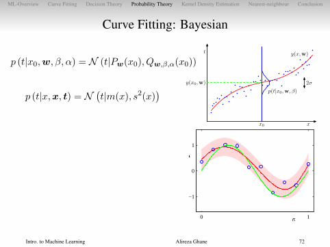
Curve Fitting: Bayesian
p (t|x0,w, β, α) = N (t|Pw(x0), Qw,β,α(x0))
p (t|x,x, t) = N(t|m(x), s2(x)
)
m(x) = φ(x)TS
N∑n=1
φ(xn)tn
s2(x) = β−1(1 + φ(x)TSφ(x)
)S−1 =
α
βI +
N∑n=1
φ(xn)φ(xn)T
t
xx0
2σy(x0,w)
y(x,w)
p(t|x0,w, β)
�
�
0 1
−1
0
1
Intro. to Machine Learning Alireza Ghane 71
ML-Overview Curve Fitting Decision Theory Probability Theory Kernel Density Estimation Nearest-neighbour Conclusion
Curve Fitting: Bayesian
p (t|x0,w, β, α) = N (t|Pw(x0), Qw,β,α(x0))
p (t|x,x, t) = N(t|m(x), s2(x)
)
m(x) = φ(x)TS
N∑n=1
φ(xn)tn
s2(x) = β−1(1 + φ(x)TSφ(x)
)S−1 =
α
βI +
N∑n=1
φ(xn)φ(xn)T
t
xx0
2σy(x0,w)
y(x,w)
p(t|x0,w, β)
�
�
0 1
−1
0
1
Intro. to Machine Learning Alireza Ghane 72

ML-Overview Curve Fitting Decision Theory Probability Theory Kernel Density Estimation Nearest-neighbour Conclusion
Curve Fitting: Bayesian
p (t|x0,w, β, α) = N (t|Pw(x0), Qw,β,α(x0))
p (t|x,x, t) = N(t|m(x), s2(x)
)
m(x) = φ(x)TS
N∑n=1
φ(xn)tn
s2(x) = β−1(1 + φ(x)TSφ(x)
)S−1 =
α
βI +
N∑n=1
φ(xn)φ(xn)T
t
xx0
2σy(x0,w)
y(x,w)
p(t|x0,w, β)
�
�
0 1
−1
0
1
Intro. to Machine Learning Alireza Ghane 73

ML-Overview Curve Fitting Decision Theory Probability Theory Kernel Density Estimation Nearest-neighbour Conclusion
Outline
Machine Learning: What, Why, and How?
Curve Fitting: (e.g.) Regression and Model Selection
Decision Theory: ML, Loss Function, MAP
Probability Theory: (e.g.) Probabilities and Parameter Estimation
Kernel Density Estimation
Nearest-neighbour
Conclusion
Intro. to Machine Learning Alireza Ghane 74

ML-Overview Curve Fitting Decision Theory Probability Theory Kernel Density Estimation Nearest-neighbour Conclusion
Histograms
• Consider the problem of modelling the distribution of brightnessvalues in pictures taken on sunny days versus cloudy days
• We could build histograms of pixel values for each classIntro. to Machine Learning Alireza Ghane 75

ML-Overview Curve Fitting Decision Theory Probability Theory Kernel Density Estimation Nearest-neighbour Conclusion
Histograms
������� ���
0 0.5 10
5
������� ��
0 0.5 10
5
������� ��
0 0.5 10
5
• E.g. for sunny days• Count ni number of datapoints (pixels) with
brightness value falling into each bin:pi = ni
N∆i
• Sensitive to bin width ∆i
• Discontinuous due to bin edges• In D-dim space with M bins per dimension,MD bins
Intro. to Machine Learning Alireza Ghane 76

ML-Overview Curve Fitting Decision Theory Probability Theory Kernel Density Estimation Nearest-neighbour Conclusion
Histograms
������� ���
0 0.5 10
5
������� ��
0 0.5 10
5
������� ��
0 0.5 10
5
• E.g. for sunny days• Count ni number of datapoints (pixels) with
brightness value falling into each bin:pi = ni
N∆i
• Sensitive to bin width ∆i
• Discontinuous due to bin edges• In D-dim space with M bins per dimension,MD bins
Intro. to Machine Learning Alireza Ghane 77

ML-Overview Curve Fitting Decision Theory Probability Theory Kernel Density Estimation Nearest-neighbour Conclusion
Histograms
������� ���
0 0.5 10
5
������� ��
0 0.5 10
5
������� ��
0 0.5 10
5
• E.g. for sunny days• Count ni number of datapoints (pixels) with
brightness value falling into each bin:pi = ni
N∆i
• Sensitive to bin width ∆i
• Discontinuous due to bin edges• In D-dim space with M bins per dimension,MD bins
Intro. to Machine Learning Alireza Ghane 78

ML-Overview Curve Fitting Decision Theory Probability Theory Kernel Density Estimation Nearest-neighbour Conclusion
Histograms
������� ���
0 0.5 10
5
������� ��
0 0.5 10
5
������� ��
0 0.5 10
5
• E.g. for sunny days• Count ni number of datapoints (pixels) with
brightness value falling into each bin:pi = ni
N∆i
• Sensitive to bin width ∆i
• Discontinuous due to bin edges• In D-dim space with M bins per dimension,MD bins
Intro. to Machine Learning Alireza Ghane 79

ML-Overview Curve Fitting Decision Theory Probability Theory Kernel Density Estimation Nearest-neighbour Conclusion
Local Density Estimation
• In a histogram we use nearby points to estimate density• For a small region around x, estimate density as:
p(x) =K
NV
• K is number of points in region, V is volume of region, N istotal number of datapoints
Intro. to Machine Learning Alireza Ghane 80

ML-Overview Curve Fitting Decision Theory Probability Theory Kernel Density Estimation Nearest-neighbour Conclusion
Kernel Density Estimation
• Try to keep idea of using nearby points to estimate density, butobtain smoother estimate
• Estimate density by placing a small bump at each datapoint• Kernel function k(·) determines shape of these bumps
• Density estimate is
p(x) ∝ 1
N
N∑n=1
k
(x− xnh
)
Intro. to Machine Learning Alireza Ghane 81
ML-Overview Curve Fitting Decision Theory Probability Theory Kernel Density Estimation Nearest-neighbour Conclusion
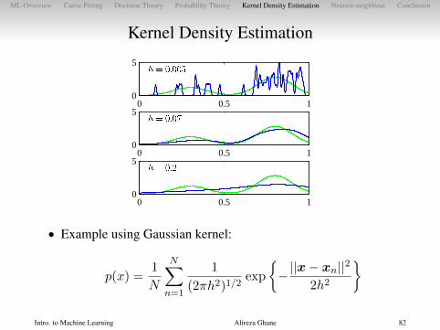
Kernel Density Estimation
������� �����
0 0.5 10
5
������� ��
0 0.5 10
5
�������
0 0.5 10
5
• Example using Gaussian kernel:
p(x) =1
N
N∑n=1
1
(2πh2)1/2exp
{−||x− xn||
2
2h2
}
Intro. to Machine Learning Alireza Ghane 82
ML-Overview Curve Fitting Decision Theory Probability Theory Kernel Density Estimation Nearest-neighbour Conclusion
Kernel Density Estimation
!3 !2 !1 0 1 2 30
0.1
0.2
0.3
0.4
0.5
0.6
0.7
0.8
0.9
1
!5 0 5 10 15 20 25 300
0.02
0.04
0.06
0.08
0.1
0.12
0.14
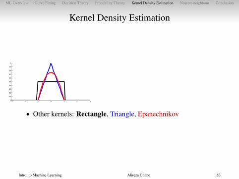
• Other kernels: Rectangle, Triangle, Epanechnikov
• Fast at training time, slow at test time – keep all datapoints• Sensitive to kernel bandwidth h
Intro. to Machine Learning Alireza Ghane 83

ML-Overview Curve Fitting Decision Theory Probability Theory Kernel Density Estimation Nearest-neighbour Conclusion
Kernel Density Estimation
!3 !2 !1 0 1 2 30
0.1
0.2
0.3
0.4
0.5
0.6
0.7
0.8
0.9
1
!5 0 5 10 15 20 25 300
0.02
0.04
0.06
0.08
0.1
0.12
0.14
• Other kernels: Rectangle, Triangle, Epanechnikov
• Fast at training time, slow at test time – keep all datapoints• Sensitive to kernel bandwidth h
Intro. to Machine Learning Alireza Ghane 84

ML-Overview Curve Fitting Decision Theory Probability Theory Kernel Density Estimation Nearest-neighbour Conclusion
Kernel Density Estimation
!3 !2 !1 0 1 2 30
0.1
0.2
0.3
0.4
0.5
0.6
0.7
0.8
0.9
1
!5 0 5 10 15 20 25 300
0.02
0.04
0.06
0.08
0.1
0.12
0.14
• Other kernels: Rectangle, Triangle, Epanechnikov• Fast at training time, slow at test time – keep all datapoints
• Sensitive to kernel bandwidth h
Intro. to Machine Learning Alireza Ghane 85

ML-Overview Curve Fitting Decision Theory Probability Theory Kernel Density Estimation Nearest-neighbour Conclusion
Kernel Density Estimation
!3 !2 !1 0 1 2 30
0.1
0.2
0.3
0.4
0.5
0.6
0.7
0.8
0.9
1
!5 0 5 10 15 20 25 300
0.02
0.04
0.06
0.08
0.1
0.12
0.14
• Other kernels: Rectangle, Triangle, Epanechnikov• Fast at training time, slow at test time – keep all datapoints• Sensitive to kernel bandwidth h
Intro. to Machine Learning Alireza Ghane 86

ML-Overview Curve Fitting Decision Theory Probability Theory Kernel Density Estimation Nearest-neighbour Conclusion
Outline
Machine Learning: What, Why, and How?
Curve Fitting: (e.g.) Regression and Model Selection
Decision Theory: ML, Loss Function, MAP
Probability Theory: (e.g.) Probabilities and Parameter Estimation
Kernel Density Estimation
Nearest-neighbour
Conclusion
Intro. to Machine Learning Alireza Ghane 87

ML-Overview Curve Fitting Decision Theory Probability Theory Kernel Density Estimation Nearest-neighbour Conclusion
Nearest-neighbour�����
0 0.5 10
5
�����
0 0.5 10
5
�������
0 0.5 10
5
• Instead of relying on kernel bandwidth to get proper densityestimate, fix number of nearby points K:
p(x) =K
NV
• Note: diverges, not proper density estimateIntro. to Machine Learning Alireza Ghane 88

ML-Overview Curve Fitting Decision Theory Probability Theory Kernel Density Estimation Nearest-neighbour Conclusion
Nearest-neighbour for Classification
x1
x2
(a)x1
x2
(b)
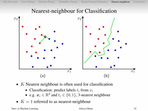
• K Nearest neighbour is often used for classification• Classification: predict labels ti from xi
• e.g. xi ∈ R2 and ti ∈ {0, 1}, 3-nearest neighbour
• K = 1 referred to as nearest-neighbour
Intro. to Machine Learning Alireza Ghane 89

ML-Overview Curve Fitting Decision Theory Probability Theory Kernel Density Estimation Nearest-neighbour Conclusion
Nearest-neighbour for Classification
x1
x2
(a)
x1
x2
(b)
• K Nearest neighbour is often used for classification• Classification: predict labels ti from xi• e.g. xi ∈ R2 and ti ∈ {0, 1}, 3-nearest neighbour
• K = 1 referred to as nearest-neighbour
Intro. to Machine Learning Alireza Ghane 90
ML-Overview Curve Fitting Decision Theory Probability Theory Kernel Density Estimation Nearest-neighbour Conclusion
Nearest-neighbour for Classification
x1
x2
(a)x1
x2
(b)
• K Nearest neighbour is often used for classification• Classification: predict labels ti from xi• e.g. xi ∈ R2 and ti ∈ {0, 1}, 3-nearest neighbour
• K = 1 referred to as nearest-neighbourIntro. to Machine Learning Alireza Ghane 91

ML-Overview Curve Fitting Decision Theory Probability Theory Kernel Density Estimation Nearest-neighbour Conclusion
Nearest-neighbour for Classification
• Good baseline method• Slow, but can use fancy data structures for efficiency (KD-trees,
Locality Sensitive Hashing)• Nice theoretical properties
• As we obtain more training data points, space becomes morefilled with labelled data
• As N →∞ error no more than twice Bayes error
Intro. to Machine Learning Alireza Ghane 92

ML-Overview Curve Fitting Decision Theory Probability Theory Kernel Density Estimation Nearest-neighbour Conclusion
Bayes Error
R1 R2
x0 x
p(x, C1)
p(x, C2)
x
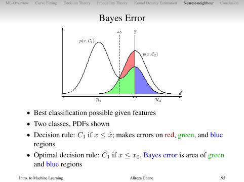
• Best classification possible given features• Two classes, PDFs shown• Decision rule: C1 if x ≤ x; makes errors on red, green, and blue
regions• Optimal decision rule: C1 if x ≤ x0, Bayes error is area of green
and blue regions
Intro. to Machine Learning Alireza Ghane 93

ML-Overview Curve Fitting Decision Theory Probability Theory Kernel Density Estimation Nearest-neighbour Conclusion
Bayes Error
R1 R2
x0 x
p(x, C1)
p(x, C2)
x
• Best classification possible given features• Two classes, PDFs shown• Decision rule: C1 if x ≤ x; makes errors on red, green, and blue
regions• Optimal decision rule: C1 if x ≤ x0, Bayes error is area of green
and blue regions
Intro. to Machine Learning Alireza Ghane 94
ML-Overview Curve Fitting Decision Theory Probability Theory Kernel Density Estimation Nearest-neighbour Conclusion
Bayes Error
R1 R2
x0 x
p(x, C1)
p(x, C2)
x
• Best classification possible given features• Two classes, PDFs shown• Decision rule: C1 if x ≤ x; makes errors on red, green, and blue
regions• Optimal decision rule: C1 if x ≤ x0, Bayes error is area of green
and blue regions
Intro. to Machine Learning Alireza Ghane 95
ML-Overview Curve Fitting Decision Theory Probability Theory Kernel Density Estimation Nearest-neighbour Conclusion
Outline
Machine Learning: What, Why, and How?
Curve Fitting: (e.g.) Regression and Model Selection
Decision Theory: ML, Loss Function, MAP
Probability Theory: (e.g.) Probabilities and Parameter Estimation
Kernel Density Estimation
Nearest-neighbour
Conclusion
Intro. to Machine Learning Alireza Ghane 96

ML-Overview Curve Fitting Decision Theory Probability Theory Kernel Density Estimation Nearest-neighbour Conclusion
Conclusion
• Readings: Chapter 1.1, 1.3, 1.5, 2.1• Types of learning problems
• Supervised: regression, classification• Unsupervised
• Learning as optimization• Squared error loss function• Maximum likelihood (ML)• Maximum a posteriori (MAP)
• Want generalization, avoid over-fitting• Cross-validation• Regularization• Bayesian prior on model parameters
Intro. to Machine Learning Alireza Ghane 97

ML-Overview Curve Fitting Decision Theory Probability Theory Kernel Density Estimation Nearest-neighbour Conclusion
Conclusion
• Readings: Ch. 2.5• Kernel density estimation
• Model density p(x) using kernels around training datapoints• Nearest neighbour
• Model density or perform classification using nearest trainingdatapoints
• Multivariate Gaussian• Needed for next week’s lectures, if you need a refresher read
pp. 78-81
Intro. to Machine Learning Alireza Ghane 98


