New Developments in 1H NMR-linked
Metabolomics: Identification of New
Biomarkers for the Metabolomic
Classification of Niemann-Pick Disease, Type
C1, and its Response to Treatment
Victor Ruiz-Rodado
Leicester, 2016
NewDevelopmentsin1HNMR-linkedMetabolomics:Identification
ofNewBiomarkersfortheMetabolomicClassificationofNiemann-
PickDisease,TypeC1,anditsResponsetoTreatment
By
VictorRuiz-RodadoAthesissubmittedinfulfilmentoftherequirementsforthedegreeofDoctorofPhilosophy
atLeicesterSchoolofPharmacy(DeMontfortUniversity).
1stSupervisor
Prof.MartinGrootveld(LeicesterSchoolofPharmacy,DeMontfortUniversity)
2ndSupervisors
Dr.CristobalJ.Carmona(LanguagesandComputerScience,DepartmentofCivilEngineering,UniversityofBurgos,Burgos,Spain)
Dr.DanielJ.Sillence(LeicesterSchoolofPharmacy,DeMontfortUniversity)
Dr.DavidElizondo(SchoolofComputerScienceandInformatics,DeMontfortUniversity)
Prof.FrancesM.Platt(DepartmentofPharmacology,UniversityofOxford)ThisPhDresearchworkwassponsoredbyDeMontfortUniversity(Leicester,UK)andHope
AgainstCancer(Leicester,UK).
Leicester,2016
ii
CONTENTS
AKNOWLEDGMENTS…………………………………………………………………………………………………………VI
DECLARATION….……………………………………………………………………………………………………………. VIII
PUBLICATIONS……………………………………………………………………………………………………………….….IX
OUTLINE………………………………………………………………………………………………………………………..……X
ABSTRACT……………………………………………………………………………………………………….……………...XIII
ABBREVIATIONS……………………………………………………………………………………………………...……… XV
LIST OF FIGURES…………………………………………………………………………………………………………….XVIII
LIST OF TABLES…..…………………………………………………………………………………………………….….…XXII
CHAPTER 1 INTRODUCTION…………………………………………………………………………………………..1
1.1. NUCLEAR MAGNETIC RESONANCE SPECTROSCOPY (NMR)…………………………………..………1
1.1.1. Water suppression experiments……………………………………………………………….…..6
1.1.2. CPMG pulse sequence…………………………………………………………………………………..8
1.1.3. Two-dimensional NMR ……………………………………………………………………………….10
1.2. METABOLOMICS………………………………………………………………………………………………………..15
1.3. MULTIVARIATE STATISTICAL ANALYSIS TECHNIQUES………………………………………………….22
1.3.1. Principal Component Analysis (PCA)…………………………………………………………….22
1.3.2. Linear Discriminant Analysis (LDA)……………………………………………………………….24
1.3.3. Partial Redundancy Analysis (pRDA)…………………………………………………………....26
1.3.4. Correlated Component Regression (CCR)…………………………………………………….27
1.3.5. ROC Curve Analysis………………………………………………………………………………………31
1.4. ARTIFICIAL INTELLIGENCE BASED TECHNIQUES………………………………………………………….32
1.4.1. Random Forests (RFs)………………………………………………………………………………….32
1.4.2. Support Vector Machines (SVMs)………………………………………………………………..33
1.4.3. Genetic Algorithms (GAs)…………………………………………………………………………….35
1.5 NIEMANN-PICK TYPE C1 DISEASE ……………………………………………………………………………….37
1.5.1. Description…………………………………………………………………………………………….......37
1.5.2. Cell biology of cholesterol……………………………………………………………………………37
1.5.3. NPC1 and NPC2 proteins……………………………………………………………………………..39

iii
1.5.4. Disease manifestations…………………………………………………………………………….….41
1.5.4.1. Hepatic manifestations …………………………………………………………………42
1.5.5. Diagnosis……………………………………………………………………………………………………..44
1.5.6. Treatment …………………………………………………………………………………………………..45
1.5.6.1. Miglustat……………………………………………………………………………………….47
CHAPTER 2 1H NMR LINKED METABOLOMICS ANALYSIS OF URINE COLLECTED FROM
NP-C1 PATIENTS, MIGLUSTAT-TREATED PATIENTS AND HETEROZYGOUS CARRIERS.....….50
2.1. URINE SAMPLE PREPARATION FOR NMR ANALYSIS…..……………………………………………….50
2.2. NMR ANALYSIS OF NP-C1 URINE SAMPLES…………………………………………………………………52
2.2.1. 1H NMR Urinary profiles of NP-C1 patients………………………………………………….53
2.2.2. Identification of bile acids in urine samples………………………………………………...57
2.3. DATA PREPROCESSING ………………………………………………………………………………………………59
2.3.1. Creatinine normalisation……………………………………………………………………………..60
2.4. UNIVARIATE AND MULTIVARIATE ANALYSIS OF THE 1H NMR URINARY DATASET……….62
2.4.1. Univariate data analysis: ANOVA……………………………………………………..………….62
2.4.2. Multivariate data analysis…………………………………………………………………..……….63
2.4.2.1. Preliminary data analysis: PCA………………………………………………..…….63
2.4.2.2. Classification performance……………………………………………………………64
2.4.2.3. Variable selection………………………………………………………………………….66
2.4.2.4. ROC curve analysis………………………………………………………………………..70
2.5. POTENTIAL AGE-CORRELATED URINARY METABOLITES………………………………………………73
2.6. NMR ANALYSIS OF URINE SAMPLES COLLECTED FROM NP-C1 PATIENTS UNDERGOING
MIGLUSTAT TREATMENT…………………………………………………………………………………………….…….74
2.6.1. NMR characterization of miglustat……………………………………………………………...74
2.6.2. Miglustat detection in urine……………………………………………………………………….. 78
2.6.3. 1H NMR analysis of urine collected from NP-C1 patients undergoing miglustat
treatment…….………………………………………………………………………………………………….……80
2.6.4. 1H NMR-linked metabolomics investigations of the response to miglustat
treatment of NP-C1 patients…………………………………………………..………………………….…85

iv
CHAPTER 3 1H NMR LINKED METABOLOMICS ANALYSIS OF PLASMA SAMPLES
COLLECTED FROM NP-C1 PATIENTS, HETEROZYGOUS CARRIERS, HEALTHY PARTICIPANTS
AND MIGLUSTAT TREATED NP-C1 PATIENTS..………………………………………………………………….90
3.1. PLASMA SAMPLES COLLECTION AND PREPARATION FOR NMR ANALYSIS……………...….90
3.2. NMR ANALYSIS OF PLASMA SAMPLES…………………………………………………………………….….91
3.2.1. 1H NMR plasma profiles of NP-C1 patients……………………………………………….….91
3.3. DATA PREPROCESSING…………………………………………………………………………………………….…95
3.4. UNIVARIATE AND MULTIVARIATE ANALYSIS OF THE 1H NMR PLASMA DATASET………..95
3.4.1. Univariate data analysis: Tukey´s HSD test…………………………………………………..95
3.4.2. Multivariate data analysis……………………………………………………………………………96
3.4.2.1. Preliminary analysis: PCA……………………….……………………………………..96
3.4.2.2. Classification performance……………………………………………………………96
3.4.2.3. Variable selection………………………………………………………………………….98
3.4.2.4. ROC curve analysis………………………………………………………………………100
3.5. 1H NMR PLASMA PROFILES OF NP-C1 PATIENTS, HETEROZYGOUS CARRIERS, HEALTHY
PARTICIPANTS AND MIGLUSTAT TREATED PATIENTS………………………………………………………101
CHAPTER 4 1H NMR LINKED METABOLOMICS ANALYSIS OF LIVER SAMPLES COLLECTED
FROM AN NP-C1 MOUSE MODEL…………………………………………………………………………………..105
4.1. LIVER AQUOEUS METABOLITES EXTRACTION FOR NMR ANALYSIS………………….……….105
4.2. NMR ANALYSIS OF LIVER EXTRACTS………………………………………………………………….……..106
4.2.1. 1H NMR hepatic profiles of NP-C1 mice……………………………………………………..107
4.3. DATA PREPROCESSING……………………………………………………………………………………………..110
4.4. UNIVARIATE AND MULTIVARIATE ANALYSIS OF THE 1H NMR MURINE HEPATIC
DATASET…………………………………………………………………………………………………………………..…….110
4.4.1. Univariate data analysis: ANCOVA……………………………………………………….…….110
4.4.2. Multivariate data analysis………………………………………………………………………….111
4.4.2.1. Preliminary analysis: PCA…………………………………………………………….111
4.4.2.2. Classification performance………………………………………………………….112
4.4.2.3. Variable selection………………………………………………………………………..113
4.4.2.4. ROC curve analysis………………………………………………………………………118
4.4.3. Time-dependency of 1H NMR NP-C1 hepatic profiles…………………………………120

v
4.4.4. Gender contribution to 1H NMR NP-C1 hepatic profiles…………………………….123
4.5. HEPATOCYTE REDOX STATUS BASED ON GSH:GSSG RATIO ……………………………………..124
CHAPTER 5 CLASSIFICATION AND VARIABLE SELECTION BY RANDOM FORESTS AND
CORRELATED COMPONENT REGRESSION IN A METABOLOMICS CONTEXT.…………………..126
5.1. RANDOM FORESTS RANKING FOR VARIABLE SELECTION VS. RANDOM FORESTS-
RECURSIVE FEATURE ELIMINATION………………………………………………………………..……………….126
5.2. CORRELATED COMPONENT REGRESSION: A NEW TOOL FOR METABOLOMICS
ANALYSIS…………………………………………………………………………………………………………………………133
5.2.1. CCR-LDA performance………………………………………..……………………………………..133
5.2.2. CCR-LDA dependency of the number of components and variables
employed…………………………………………………………………………………………………..………..134
CHAPTER 6 INTEGRATIVE METABOLOMICS: URINE, PLASMA AND LIVER TO ASSESS THE
METABOLISM OF NP-C1 PATIENTS….……………………………………………………………………………..138
6.1. NICOTINATE/NIACINAMIDE PATHWAY ……………………………………………………………..…….138
6.2. BLOOD PLASMA LIPOPROTEIN PROFILES………………………………………………………………….142
6.3. BILE ACIDS METABOLISM…………………………………………………………………………………………144
6.4. MUSCLE BIOMASS WASTING……………………………………………………………………………………146
6.5. GUT MICROFLORA IN NP-C1 DISEASE……………………………………………………………………….150
6.6. HEPATIC STATUS IN NP-C1 DISEASE………………………………………………………………………….153
6.7. BIOMARKERS FOR NP-C1 DISEASE…………………………………………………………………………….159
CHAPTER 7 CONCLUSIONS…………………………………………………………………………………………165
APPENDIX 1 QUANTIFICATION OF MIGLUSTAT AND 1-O-VALPROIL-β-GLUCURONATE IN
URINE SAMPLES COLLECTED FROM NP-C1 PATIENTS UNDERGOING MIGLUSTAT
TREATMENT…….….………………………………………………………………………………………………………….172
REFERENCES………..………………………………………………………………………………………………………….179

vi
AKNOWLEDGEMENTS
Firstly, I would like to thank Prof. Martin Grootveld for giving me the opportunity of
starting a career in Research, for his supervision throughout this work and for his help, not
only in Research matters but also providing his support with personal issues, together with
his wife, Kerry.
I would also like to thank the rest of my supervisory team, namely Dr. David Elizondo,
Dr. Dan Sillence, and specially Prof. Fran M. Platt, for kindly hosting me every time I came
down to her lab at University of Oxford. Thanks to Dr. Raluca Nicoli from Platt Lab for taking
care of me every time I was there and helping with all the animal work. Thanks to Dr. Fay
Probert for the useful discussions about this project and her help in some of the work
described herein.
Since this project involved different research groups, I would like to thank them all
for their help in the provision of biological samples, including those at Section on Molecular
Dysmorphology (NIH, Bethesda, USA), National Hospital for Neurology and Neurosurgery
(London, UK), The Mark Holland Metabolic Unit (Salford, UK) and St. Mary’s Hospital
(Manchester, UK).
Also thanks to the sponsors that funded this research work: De Montfort University
for the fees scholarship award and Hope Against Cancer (Leicester, UK) for the provision of
stipend.
Many thanks to Dr. Mark Edgar for taking the time to train me on NMR at
Loughborough University.

vii
Special thanks to the small Spanish family that we created here in Leicester
throughout these 4 years, for creating the feeling that we were still at home and to put up
with all the scientific problems that I unfortunately (for them) shared with them.
Many special thanks to my parents, Manuel and Carmen, to my brother Carlos, and
more specially to my grandmother Lola, since in a very weird way she always knew that I was
going to work in science. Thanks for their support and patience, and for making me feel that
I never left Madrid in each Skype talk and every visit.
Finally, but by no means least, I would like to thank my awesome wife, Bea. She
started all this, encouraging me to go through this PhD process, providing her support at any
step and being involved in any achievement that we might have; since any good that
subsequently happens is mainly because of her. Thanks as well for her ‛interest’ in NMR,
metabolomics and ‛that Niemann whatever’ that she had to explain every time someone
asked. This work (as everything else) is dedicated to her.

viii
DECLARATION
This thesis has not been accepted in any previous application for a degree and
contains the original work of the author except where otherwise indicated.
Patient recruitment and sample collection
The personnel involved in the NP-C1 urine sample collection included Danielle te
Vruchte (Department of Pharmacology, University of Oxford, UK), Dr. Robin H. Lachmann
(National Hospital for Neurology and Neurosurgery, London, UK), Prof. Christopher J.
Hendriksz (The Mark Holland Metabolic Unit, Salford, UK), Dr. James E. Wraith (St. Mary’s
Hospital, Manchester, UK) and Jackie Imrie (St. Mary’s Hospital, Manchester, UK).
All plasma samples used in this study were collected under the Eunice Kennedy
Shriver National Institute of Child Health and Human Development Institutional Review
Board (Principal Investigator: Dr. Forbes D. Porter). The collections took place at the National
Institutes of Health clinical centre in Bethesda, Maryland, USA.
Plasma separation from ‛whole blood’ was performed by Danielle te Vruchte
(University of Oxford, Oxford, UK).
Animal work and liver tissue collection was performed by Dr. Raluca Nicoli (University
of Oxford) at University of Oxford.
Data Analysis
Data analysis performed on the urine samples collected from NP-C1 patients
undergoing miglustat treatment and that performed on plasma samples was done in
conjunction with Dr. Fay Probert.
ix
PUBLICATIONS
Probert, F., Ruiz-Rodado, V., Zhang, X., te Vruchte, D., Claridge, T. D., Edgar, M., Zonato Tocchio, A.,
Lachmann R. H., Platt, F. M., Grootveld, M. Urinary excretion and metabolism of miglustat and
valproate in patients with Niemann–Pick type C1 disease: One-and two-dimensional solution-state
1H NMR studies. Journal of pharmaceutical and biomedical analysis, 2016, Vol. 117, 276-288.
Ruiz-Rodado, V., Luque-Baena, R. M., te Vruchte, D., Probert, F., Lachmann, R. H., Hendriksz, C. J.,
Wraith, J. E., Imrie, J., Elizondo, D., Sillence, D., Clayton, P., Platt, F. M., Grootveld, M. 1H NMR-Linked
Urinary Metabolic Profiling of Niemann-Pick Class C1 (NPC1) Disease: Identification of Potential New
Biomarkers using Correlated Component Regression (CCR) and Genetic Algorithm (GA) Analysis
Strategies. Current Metabolomics, 2014, Vol. 2, 88-121.

x
OUTLINE
This thesis describes the applications of NMR-linked metabolomics analysis to urine
and plasma samples collected from human Niemann Pick, type C1, (NP-C1) patients and their
corresponding controls, together with the analysis of hepatic tissue from a mouse model of
this disease, in order to explore metabolic alterations arising from the disease process, and
also to seek valuable biomarkers for the purpose of diagnosing and monitoring its
progression.
The first Chapter (Chapter 1) provides an introduction to the main techniques
employed in this work. A summary of NMR theory has been included in order to explain how
this analytical technique operates, its applicability to the field of biofluid and tissue samples
analysis, and how useful it is as a diagnostic tool. The field of metabolomics will also be
described, together with the historical evolution of the methodologies employed. Chapter 1
is also focused on the disease of study, Niemann-Pick, type C1 (NP-C1). The biochemical
processes underlying this disease, the pathophysiological manifestations experienced by
afflicted patients (with special reference to liver dysfunction and damage), together with the
current status of treatment, specifically that involving the pharmacological agent miglustat,
and disease diagnosis will be also explained.
Chapter 2 describes the resolution of the urinary 1H NMR profile of NP-C1 patients,
which is of major utility in the metabolomics-linked data analysis performed. The
information extracted therefrom was subjected to differing multivariate analysis (MVA)
strategies in order to classify these patients according to their disease status. Indeed, ROC
curve analysis was employed for the purpose of assessing the classification success rate of

xi
the models developed for this urinary dataset in order to seek valuable biomarkers for this
lysosomal storage disease. NMR analysis of urine samples from NP-C1 patients receiving
therapies such as miglustat was also explored in order to detect this agent in their urinary 1H
NMR profiles; accordingly, the solution structure of this drug was also investigated by NMR
analysis.
Chapter 3 outlines the 1H NMR-linked metabolomics analysis performed on blood
plasma samples collected from NP-C1 patients, healthy individuals, heterozygous disease
carriers, together with NP-C1 patients undergoing miglustat treatment. The Random Forests
(RFs) strategy was employed to classify these samples based on their classifications. A brief
discussion regarding the methodology employed for the acquisition of 1H NMR spectra on
these samples is also included. Finally, comparisons between the 1H NMR plasma profiles
acquired from all the different patients/participants in the study are conducted, along with
an evaluation of plasma metabolites as possible NP-C1 disease biomarkers.
Chapter 4 describes the NMR analysis performed on liver samples collected during
the development of NP-C1 in a mouse model of the disease, since this organ plays a crucial
role in this disorder. The dataset extracted from the multicomponent 1H NMR analysis of
aqueous extracts of these samples were analysed by RFs in order to extract valuable
information regarding the disease classification of these hepatic tissue extracts. Additionally,
the correlation of such metabolic changes to the progression of the disease was investigated,
in addition to the redox status of the hepatic tissue.
In Chapter 5, the ability of a newly-developed statistical MVA method, Correlated
Component Regression, to successfully perform in a metabolomics context was evaluated,
along with its dependence on the number of variables and components employed to build

xii
such classification models, specifically those arising from the urinary and hepatic NP-C1
datasets. Both datasets will also serve to compare the variables ranking obtained after a
cross-validated RFs analysis to a Recursive Feature Elimination (RFE) variant of the same
method for variable selection.
In Chapter 6, all the metabolic pathways and biochemical processes that can be
affected in NP-C1 disease process are discussed according to the outcomes obtained in the
previous sections, and will be compared and contrasted with corresponding information
available in the literature. Furthermore, some metabolites will be proposed as valuable
biomarkers for the diagnosis and stratificational prognosis of NP-C1 disease.
In Chapter 7 the conclusions arising from this work will be discussed, including the
utility of the metabolites selected as discriminatory urinary and blood plasma biomarker
features for the diagnosis of NP-C1, together with outcomes from the NMR analysis of liver
tissue samples. The classificational abilities of the RFs-Recursive Feature Elimination and
CCR-LDA MVA strategies in a metabolomics context is also delineated.
xiii
ABSTRACT
NMR-linked metabolomics analysis was employed to investigate urinary and human
plasma profiles collected from Niemann Pick type C1 disease patients (NP-C1), in addition to
aqueous extracts of liver samples of an NP-C1 mouse model. NP-C1 is a lysosomal storage
disorder caused by mutations in the lysosomal proteins NPC1 and NPC2, which are involved
in lysosomal cholesterol trafficking. NP-C1 disease is a fatal genetic disorder, characterised
by neurodegeneration and hepatic damage. Miglustat (MGS) is the only approved drug for
this disease, and consequently, plasma and urine samples collected from MGS-treated
patients were also investigated.
The ability of 1H NMR analysis to detect a wide range of metabolites simultaneously
served to characterize the metabolic profiles of urine, plasma and hepatic tissue samples
investigated in order to perform linked multivariate analysis (MVA). Additionally, MGS was
identified in urine samples collected from NP-C1 treated patients. MVA employing both
parametric and machine learning-based techniques was conducted to classify samples
according to their disease status, and also to seek biomarkers that could aid in the diagnosis
and/or prognosis of the disease. Moreover, a new technique was introduced in a
metabolomics context, Correlated Component Regression (CCR), and the suitability of
Random Forests (RFs) for variable selection was also explored.
We were able to differentiate urine samples collected from NP-C1 patients from
those collected from heterozygous controls, and also propose several metabolites as NP-C1
urinary biomarkers such as bile acids, 2-hydroxy-3-methylbutyrate, 3-aminoisobutyrate, 5-
aminovalerate, trimethylamine, methanol, creatine and quinolinate. The 1H NMR linked

xiv
metabolomics study of plasma samples revealed major distinctions among the groups
investigated, metabolic alterations ascribable to the disease pathology were mainly
observed as changes in the lipoprotein profiles of NP-C1 patients. Hepatic tissue extracts
analysed revealed major disturbances in amino acid metabolism, along with impairments in
the NAD+/NADH production and redox status. Gut microbiota and bile acid metabolism were
also highlighted as features altered in NP-C1 disease.
CCR linked to Linear Discriminant Analysis was evaluated as a new tool for
metabolomics analysis, giving accurate results when compared to alternative techniques
tested. Additionally, the suitability of Random Forests and associated recursive feature
elimination for variable selection in metabolomics studies was contrasted, suggesting that
those strategies relying on a variable ranking to select the top features for discrimination are
more suitable for metabolomics investigations than those that iteratively remove a
percentage of the least effective features until the classification performance decays.
xv
ABBREVIATIONS
3-AIB (3-aminoisobutyrate)
AA (Amino Acid)
AAA (Aromatic Amino Acid)
ACC (Accuracy)
ANCOVA (Analysis Of Covariance)
ANOVA (Analysis Of Variance)
AUC (Area Under the Curve)
BA (Bile Acid)
BBB (Blood Brain Barrier)
BCAA (Branched Chain Amino Acid)
BMRB (Biological Magnetic Resonance Data Bank)
BRP (Between Run Precision)
CCR (Correlated Component Regression)
CI (Confidence Interval)
Cn (CreatiNine)
COSY (Correlation Spectroscopy)
Cr (CReatine)
CV (Cross-Validation)
DG (DiacylGlicerides)
DMA (DiMethylAmine)
EMA (European Medicines Agency)
ER (Endoplasmic Reticulum)
FDA (Food and Drug Administration)
FID (Free Induction Decay)
FA (Fatty Acid)
FT (Fourier Transform)
GAs (Genetic Algorithms)
GC (Gas Chromatography)
HDL (High Density Lipoproteins)
xvi
HMDB (Human Metabolome Data Base)
HSQC (Heteronuclear Single Quantum Coherence)
INEPT (Insensitive Nuclei Enhanced by Polarization Transfer)
LC (Liquid Chromatography)
LDA (Linear Discriminant Analysis)
LDL (Low Density Lipoproteins)
LLOQ (Lower Limit Of Quantification)
LOD (Limit Of Detection)
MCCV (Monte Carlo Cross-Validation)
MLHD (Maximum LikeliHooD)
MS (Mass Spectrometry)
MVA (MultiVariate Analysis)
NAD (Nicotinamide Adenine Dinucleotide)
NADP (Nicotinamide Adenine Dinucleotide Phosphate)
NAFLD (Non-Alcoholic Fatty Liver Disease)
Nampt (NicotinAMide PhosphoribosylTransferase)
NMDA (N-Methyl-D-Aspartate)
NMR (Nuclear Magnetic Resonance)
NOESY (Nuclear Overhauser Effect SpectroscopY)
NP-C (Niemann Pick type-C)
OM (Overall Mean)
OOB (Out-Of-Bag)
PCA (Principal Component Analysis)
pRDA (Partial Redundancy Analysis)
QC (Quality Control)
QUIN (quinolinate)
RFs (Random Forests)
ROC (Receiver Operating Characteristic)
SE (Standard Error)
SPE (Solid Phase Extraction)
SVMs (Support Vector Machines)
TG (TriacylGlicerides)

xvii
TMA (TriMethylAmine)
TMAO (TriMetylAmine-N-Oxide)
TOCSY (Total Correlation Spectroscopy)
TNR (True Negative Rate)
TPR (True Positive Rate)
TSP (TrimethylSilyl Propanoic acid)
VLDL (Very Low Density Lipoproteins)
WRP (Within Run Precision)

xviii
LIST OF FIGURES
Figure 1.1. (a) Energetic sublevels present when a nucleus with non-zero spin is placed
into a magnetic field. (b) Precession movement of nuclei around the z-axis at which B0 has
been applied. (c) Direction of the magnetization vector My in the rotating frame system…..4
Figure 1.2. Stack plot of a 1D plasma spectrum acquired through a (a) NOEPR pulse
sequence and acquired through a (b) CPMG pulse sequence with water suppression…….…10
Figure 1.3. Energy levels scheme and transitions for a two spin system AX conformed for
two +H…………………………………………………………………………………………………………………………….…12
Figure 1.4. 16th Century diagnostic urine wheel published in 1506 by Ullrich Pinder, in his
book Epiphanie Medicorum…………………………………………………………………………………………….…16
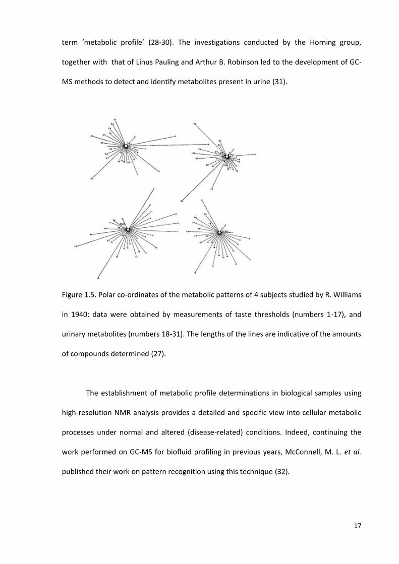
Figure 1.5. Polar co-ordinates of the metabolic patterns of 4 subjects studied by R.
Williams in 1940………………………………………………………………………………………………..………..…….17
Figure 1.6. Experiment performed by Hoult et al. involving 31P-NMR analysis (129 MHz)
of muscle.………………………………………………………………………………………………………………………...18
Figure 1.7. PCA representation in a 3D space……………………………………………………..…….….23
Figure 1.8. Matrix representation of a PCA model………………………………………………………..24
Figure 1.9. Schematic representation of GAs procedure for a classification problem…..36
Figure 1.10. Potential mechanism for NPC1/NPC2-mediated cholesterol export from
LE/L………………………………………………………………………………………………………………………….……….40
Figure 1.11. Major clinical disease manifestations and age at onset of neurological
symptoms of NP-C1…………………………………………………………………………………………………….…….42
Figure 1.12. Key steps in the biosynthesis of GSLs………………………………………..……….………48
xix
Figure 2.1. (a), (b) and (c), 0.50-2.75, 2.75-5.50 and 6.00-9.50 ppm regions, respectively,
of the 600 MHz urinary 1H NMR profile of an NP-C1 patient……………………………………………..54
Figure 2.2. 400 MHz 1D-TOCSY spectrum of a human urine specimen collected from an
NP-C1 disease patient…………………………………………………………………………………………….…………57
Figure 2.3. (a) 0.4 - 1.1 ppm region from a 400 MHz 1H NMR spectra of a urine sample
‛spiked’ with different bile acids (BAs) (b) BAs general chemical structure together with a
table listing those BAs arising from the different possible substitutions in those groups
highlighted……………………………………………………………………………………………………………….……….58
Figure 2.4. Box plot for Cn signal (4.05 - 4.10 ppm)………………………………………….………….61
Figure 2.5. PCA 3D score plot for the NP-C1 urinary dataset……………………..………………..63
Figure 2.6. (a) ROC curves and (b) bubbles diagram for variable importance in the NP-C1
urinary dataset………………………………………………………………………………………………………….……...71
Figure 2.7. Assigned 1D 1H-NMR spectrum of MGS 20 mM in 17.0 mM phosphate buffer,
pH 7.10 (90% H2O/10% D2O)……………………………………….…………………………….……………….…….75
Figure 2.8. (a) 400 MHz 1H-1H COSY and (b) 1H-13C HSQC spectrum of 20 mM MGS in 17.0
mM phosphate buffer, pH 7.10 (90%/10% D2O/H2O)…………………………………………..…………..77
Figure 2.9. 400 MHz 1D spectra of urine collected from an NP-C1 patient before (b) and
after (a) MGS treatment; (c) healthy urine sample spiked with MGS and (d) the same urine
sample untreated………………………………………………………………………………………………….………….79
Figure 2.10. 400 MHz 1D spectra of urine collected from an NP-C1 patient before (b) and
after (a) MGS treatment; (c) healthy urine sample spiked with MGS (red) and the same urine
sample untreated…………………………………………………………..…………………………………….…….…….81
Figure 2.11. Aromatic region from a 1H-NMR 400 MHz urine spectra collected from a NP-
C1 MGS-treated patient treatment before (b) and after (a) β-glucuronidase incubation…..84
Figure 2.12. Analysis of discriminatory metabolites levels amongst heterozygotes controls
(HET), NP-C1 patients (NPC) and MGS-treated NP-C1 patients (MGS)………………………………86

xx
Figure 3.1. Stack plot of (a) a plasma sample separated by histopaque and (b) a water
sample also passed through a histopaque column…………………………………………………………….93
Figure 3.2. (a) 0.75 - 4.45 and (expansion of the BCAA region is included as an insert) (b)
5.10 - 8.50 ppm regions from an NP-C1 patient 1H NMR plasma profile……………………………94
Figure 3.3. PCA scores plots for PC1 vs. PC2 for each pair of comparisons, and
multidimensional scaling plot from a RFs proximity matrix showing success of discrimination
from a single RFs iteration for the NP-C1 plasma dataset………………..………………………..………98
Figure 3.4. (a) ROC curves and (b) bubble diagram for variable importance for the NP-C1
blood plasma dataset……………………………………………………………………………………………………...101
Figure 3.5. Box plots for metabolites selected in more than one classification problem for
the NP-C1 plasma dataset……………………………………………………………………………….……..……….102
Figure 4.1. 1H NMR spectrum of an NP-C1 mouse liver aqueous extract………………….…109
Figure 4.2. (a) Three-Dimensional (3D) PC4 vs. PC3 vs. PC2 scores plot arising from PCA
of the liver NP-C1 dataset (b) Multidimensional scaling plot of a random forests proximity
matrix from HET/WT vs. NPC analysis……………………………………………………………….………..…..112
Figure 4.3. 400 MHz 1H-13C HSQC spectrum of an NP-C1 mouse liver aqueous
extract…………………………………………………………………………………………………………………………….116
Figure 4.4. 400 MHz 1H-1H COSY spectrum, of an aqueous extract of an NP-C1 liver
sample. Typical spectra is shown………………………………………………………………………….…………117
Figure 4.5. (a) ROC curves analysis for the liver NP-C1 dataset and (b) bubble diagram for
variable importance for the NP-C1 mice hepatic dataset……………………………………..………….119
Figure 4.6. Box and whisker plots of the 11 metabolites identified as discriminatory
variables for the NP-C1 liver dataset by RFs analysis vs. time-point (weeks) for the NPC and
HET/WT classifications………………………………………………………………………………………………….…122
Figure 4.7. Typical spectra from an aqueous liver tissue extract from 3.15 ppm to 4.62
ppm showing the resonance signals employed for the [GSH]:[GSSG] computation…..…….125

xxi
Figure 4.8. (a) Box plot for hepatic mice GSH:GSSG ratio [4.55 - 4.61]:[3.31 - 3.35] and
(b) for hepatic mice GSH levels for both disease classification groups………………..…………..125
Figure 5.1. (a) MDA values for top-5 variables ranked by RFs over 100 iterations. (b)
Recursive Feature Elimination (RFE) for the urinary NP-C1 dataset………………………………….127
Figure 5.2. (a) Mean decrease in accuracy (MDA) values computed for the 5 most
effective discriminatory variables throughout 100 iterations. (b) Recursive Feature
Elimination (RFE) for the mice liver NP-C1 dataset………………………………………………………….129
Figure 5.3. CCR-LDA results for the NP-C1 urinary dataset. (a) Scatter plot of the number
of variables vs. the parameters employed. (b) Mean values for specificity (Spec), sensitivity
(Sen), accuracy (Acc) and area under the curve (AUC) along with their SEM values. (c)
Individual density plots for specificity, sensitivity, accuracy and AUC as a function of the
number of variables employed by CCR-DA………………………………………………………………………135
Figure 5.4. CCR-LDA results for the NP-C1 mice hepatic dataset. (a) Scatter plot of the
number of variables vs. the parameters employed. (b) Mean values for specificity (Spec),
sensitivity (Sen), accuracy (Acc) and area under the curve (AUC) along with their SEM values.
(c) Individual density plots for specificity, sensitivity, accuracy and AUC as a function of the
number of variables employed by CCR-DA……………………………………………………..………..……..136
Figure 6.1. NAD+ metabolism…………………………………………………………………………………….140
Figure 6.2. Bile acid synthesis pathway……………………………………………………………………..145
Figure 6.3. BCAA degradation metabolic pathway…………………………………………………….148
Figure 6.4. Enzymatic biotransformation of 3-hydroxyphenylacetate to 3,4-
dihydroxyphenylacetate………………………………………………………………………………….………………158
Figure A1. Non-treated urine samples spiked with MGS…………………..……………………….175
Figure A2. Standard addition experiments for MGS-treated urine samples……………….177

xxii
LIST OF TABLES
Table 1.1. General confusion matrix………………………………………………………..…………………31
Table 2.1. General characteristics of participants included in the urinary NP-C1
metabolomics investigation…………………………………………………………………………………………..….51
Table 2.2. Classification performance of the techniques employed for the analysis of the
NP-C1 urinary ataset……………………………………………………………………………………….……….……….65
Table 2.3. Discriminatory variables for the urinary NP-C1 dataset…………………………..….67
Table 2.4. Chemical shifts together with the coupling patterns and coupling constants
for 1H and 13C NMR spectra acquired on MGS in aqueous media………………………………………76
Table 2.5. Reported methods for valproate and/or its metabolites quantification and
detection in biofluids and tissue……………………………………………………………………..………………...82
Table 2.6. List of discriminatory variables with resonance signals overlapping those
arising from drugs and corresponding metabolites found in urine samples collected from NP-
C1 patients receiving MGS treatment……………………………………………………………….……………….85
Table 3.1. Participants’ information included in the NP-C1 plasma dataset...………….….91
Table 3.2. RFs classification performance for all 4 groups analysed in the plasma dataset:
tables showing mean and SEM values (the latter between brackets) for OOB error (a),
accuracy (b), sensitivity (c) and specificity (d) values………………………………………………………….97
Table 3.3. RFs discriminatory variables for the NP-C1 plasma dataset…………………….….99
Table 4.1. Liver samples available for 1H NMR-linked metabolomics analysis at time-
points of 3, 6, 9 and 11 weeks……………………………………………………………………………………..….106

xxiii
Table 4.2. Key 1H NMR variables derived from the application of RFs on the liver NP-C1
dataset……………………………………………………………………………………………………..…………….………114
Table 5.1. MVA performance of all the technique employed for the urinary and liver NP-
C1 datasets…………………………………………………………………………………………………………..…………133
Table A1. Background contribution (matrix effect) to MGS concentration calculations on
selected urine samples…………………………………………………………………………………………….………176
Table A2. Within-run (WRP) and between-run precision (BRP) estimates (%) for 1H NMR
determinations of miglustat (MGS) and 1-O-valproyl-β-glucuronide………………………………..178
1
CHAPTER 1
INTRODUCTION
1.1. NUCLEAR MAGNETIC RESONANCE SPECTROSCOPY (NMR)
NMR is a spectroscopic technique based on the magnetic properties of nuclei. The
effect of the magnetic field on the nuclei was first discovered by Rabi et al. in 1939 (1), when
he performed an experiment based on sending a stream of hydrogen atoms through an
homogeneous magnetic field which was additionally subjected to a radiofrequency field;
these researchers found that some energy was absorbed by the molecules at a defined
frequency, and this absorption caused a small-but-detectable deflection of the beam (1).
This was the first observation of NMR, and Rabi received the Nobel Prize in 1944 based on
his contribution towards the birth and development of this technique.
Nuclear spin (I) is an intrinsic form of angular momentum (p) possessed by atomic
nuclei which contain an odd number of protons or neutrons. The value of I is characteristic
for each isotope.
𝑝 = 𝐼ℎ
2𝜋 (1)
2
A proton has a spin associated about an axis, which is a form of angular momentum,
p. This spin presents an associated magnetic moment, μ. The correlation between both
parameters is given by the gyromagnetic ratio, γ.
𝛾 =𝜇
𝑝 (2)
Without a magnetic field, nuclear spin are orientated randomly; however, when the
sample is placed in an external magnetic field, nuclei with positive spin are orientated in the
same direction as this magnetic field, in the minimum energy state. However, nuclei with
negative spin are orientated in the opposite direction, and this anti-parallel orientation has
the higher energy. This effect on the orientation of nuclei in a magnetic field is known as the
Zeeman Effect.
When a bulk sample of hydrogen nuclei (protons) is placed in a magnetic field, it is
expected that such particles are distributed equivalently, following the Boltzmann
distribution, in both low and high energy states, through their parallel and anti-parallel spin
orientations. The allowed orientations (m) are determined by the relation 2I + 1, and which
is described by the magnetic quantum number, which takes values from -I to +I. For instance,
in the proton case where I = 1/2, then m assumes values of -1/2 and +1/2. However, after a
certain time (known as relaxation time), this sample of protons will attain thermal
equilibrium with respect to the magnetic field (2).
It is possible to induce the movement from the lower energy state to the higher
energy state by applying radiation in the radiofrequency region to the sample. The energy of
this transition, and hence, the frequency associated with it, and which is absorbed by the
nuclei to accomplish the transition to the higher energy state, is given by the Bohr condition:
3
𝜈 =𝛾𝐵0
2𝜋 (3)
The nucleus under the magnetic field B0 along the z-axis (in this case) draws a
precession movement around this axis [Figure 1(b)] since the alignment with Bo cannot be
completely achieved. The angle has a defined value since it is quantizated (cos θ = m/I). The
angular velocity of this precession movement is given by the Larmor equation:
𝜔0 = 𝛾𝐵0 (4)
This radiation has the same energy as the differing orientations, which is the
resonance frequency of the system, known as Larmor frequency. In order to detect this
effect, a vector M0 (magnetization vector) must be rotated away from z-axis towards the x,y-
plane. In view of the strong B0 applied to the sample, the only means to displace M0 is to
supply an RF pulse orthogonal to B0 (along the x-axis) oscillating at the Larmor frequency of
our nuclei, i.e. achieving resonance (3). This pulse is known as a 90o pulse [Figure 1(c)], since
it rotates the magnetization 90o. Once the magnetization has been transferred to the x,y-
plane, and therefore nuclei are precessing about it, the electrical current generated can be
detected by a receiver coil.
Resonance causes transitions between both energy states [Figure 1(a)], and
therefore nuclei can move to the maximum energy state. These two orientations are termed
α (m = ½) and β (m = -½) respectively. Since more protons will have the lower-energy parallel
orientation, a radio signal at the resonance frequency will be absorbed, and hence generate
more upward transitions. When nuclei return to their minimum energy state, they are
4
required to lose that energy since it is a non-equilibrium state; subsequently, they emit the
electromagnetic signal, termed Free Induction Decay (FID), which is detected by the receiver
coil. The loss of this energy is conditioned by two parameters, T1 and T2. T1 is the spin-lattice
or longitudinal relaxation time which leads to the recovery of Mz (achievement of thermal
equilibrium); and T2 is the spin-spin or transverse relaxation time which involves the decay
of the Mxy magnetization.
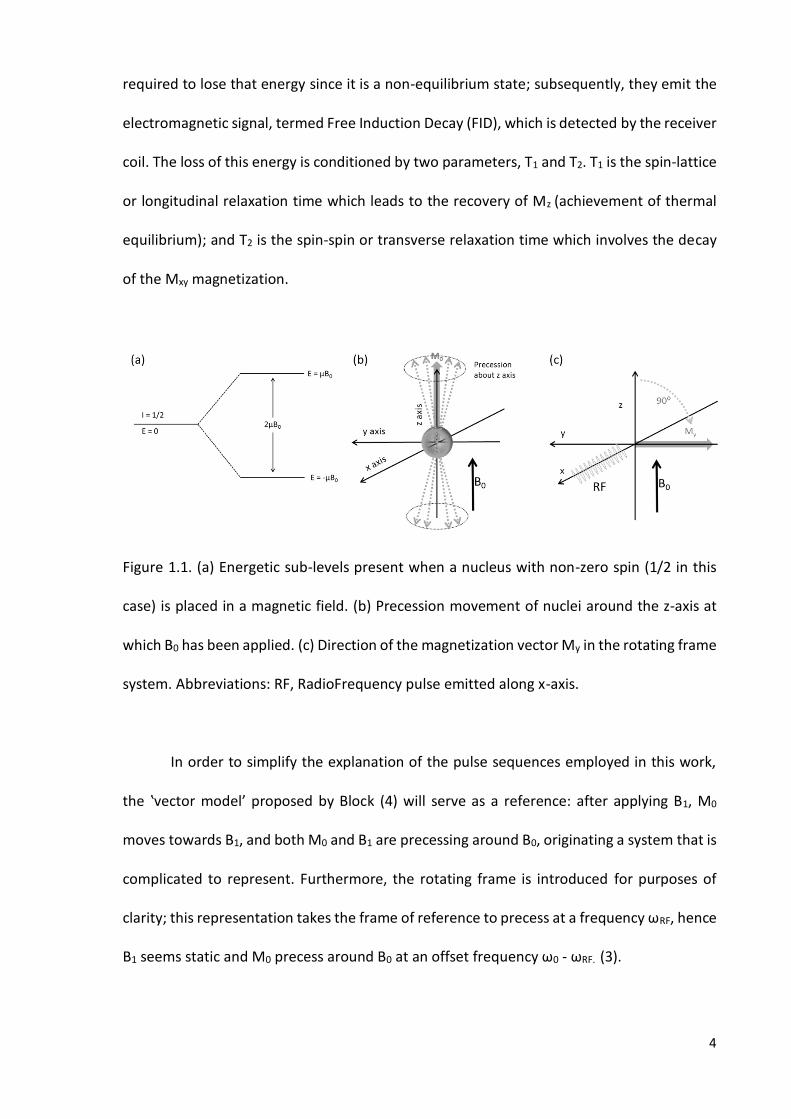
Figure 1.1. (a) Energetic sub-levels present when a nucleus with non-zero spin (1/2 in this
case) is placed in a magnetic field. (b) Precession movement of nuclei around the z-axis at
which B0 has been applied. (c) Direction of the magnetization vector My in the rotating frame
system. Abbreviations: RF, RadioFrequency pulse emitted along x-axis.
In order to simplify the explanation of the pulse sequences employed in this work,
the ‛vector model’ proposed by Block (4) will serve as a reference: after applying B1, M0
moves towards B1, and both M0 and B1 are precessing around B0, originating a system that is
complicated to represent. Furthermore, the rotating frame is introduced for purposes of
clarity; this representation takes the frame of reference to precess at a frequency ωRF, hence
B1 seems static and M0 precess around B0 at an offset frequency ω0 - ωRF. (3).

5
The subsequent Fourier Transform (FT) of the FID provides a normal NMR spectrum
with absorption signals at frequencies that represent the energy difference between the
basal and excited states (2). This operation was implemented in 1966 by Anderson and Nerst
(5), and was based in the previous discoveries made by Lowe and Norberg in 1957 (6). In
summary, this transformation converts a signal described as a function of time into one
within the frequency domain.
In nuclear magnetism, not only are the nuclei involved, but also the electrons
surrounding them, and these electronic effects are responsible for the differences in the
locations of the resonances in conventional spectra. Nuclei’s behaviours in the magnetic field
can be influenced by different effects, providing information such as:
Environment and atoms linked to each nucleus (chemical shift, δ): In molecules, the
nuclei are magnetically-deshielded or -shielded; the effective field at the position of nuclei is
different from the externally-applied field. This phenomenon is attributable to the
distribution of ‛electron density’ within the molecule, mainly around the protons and bonds
involving these. Those groups with more electronic density around themselves experience
an effective magnetic field lower than the one originally applied, this is the case for the
methyl group at the terminus of a hydrocarbon chain, for example. Contrarily, those groups
with less electronic density experience a more intense magnetic field (≤ B0, though), so that
they are deshielded, such as those adjacent to carbonyl groups. The chemical shifts are
therefore considerably affected by substituents which specifically influence this electron
distribution; for instance, electronegative groups will pull away the electrons of
neighbouring groups towards themselves, generating a deshielding effect, and therefore
giving rise to a more downfield-shifted signal.
6
Number of nuclei (peak integral): The relative intensity from a resonance signal can
be correlated with the number of nuclei that generate that signal. It is therefore possible to
quantitatively estimate the proportions of different protons within the molecule, and this
involves determinations of the area under the resonance peak.
Number and placement of nuclei (multiplicity): In view of the electronic distributions
in a bond, two linked nuclei retain the spin information of each other. The energy difference
between the two energy levels is modified by the other nuclei, and therefore if electrons of
one nucleus are in the excited state (higher energy level), the energy difference of
contiguous nuclei will be increased, and vice-versa. Furthermore, two different energy sub-
levels will appear for each case, both of them higher or lower than the initial state. This
phenomenon is known as spin-spin coupling, and consequently, the splitting of resonances
is observed. The separation between the different multiplet lines of the same resonance
signal is known as the coupling constant, J. It is calculated as the distance in Hz between
these resonance lines.
1.1.1. Water suppression experiments
A simple pulse sequence involves the application of a 90o pulse (this value can be
diminished to speed up the experiment) followed by the data acquisition, in which the FID is
recorded. However, in NMR-linked metabolomics studies, the presence of water in the
samples investigated is a common issue, since serum, urine, cerebrospinal fluid (CSF), etc.,
are all water-based biofluids. The relative concentration of metabolites in these fluids is
minimal when compared to that of water, and therefore, the signal arising from H2O
dominates the majority of the 1H single pulse spectra. In order to overcome this issue, water

7
suppression experiments are employed. The pulse sequences utilised in these experiments
remove (partially) the water signal through different approaches. Two of the most commonly
employed techniques used in metabolomics are NOEPR (Nuclear Overhauser Effect pulse
train with presaturation during relaxation and mixing time) (7), and PRESAT (Presaturation)
(8). Single-pulse spectra without suppression of the solvent signal present the main issue of
signal overlap, and also overloading of the receiver, generating baseline distortions (wiggles)
if the receiver gain value is very high, or inadequately digitized signals if this value is set very
low to allow the acquisition of the massive solvent peak (9).
PRESAT: This is a two-pulse experiment that utilizes a relatively long (seconds), low
power RF pulse to selectively saturate (the solvent) at a specific frequency by irradiating
during the relaxation delay (RD), and with a non-selective pulse to excite the full spectrum
of resonances (8). The long power pulse is of the order of the solvent T1, so that it does not
allow it to relax, and consequently its signal is suppressed. As noted above, this presaturation
pulse is relatively long, so that the hydrogen atoms of -OH, -NH and -NH2 groups that
chemically exchange with water are also saturated, and therefore they are unobservable or
attenuated (for instance, the urea signal detectable in urine) (10). The pulse sequence works
as follows: Presat (RD) - 90ox. It should be noted that the duration of a pulse is inversely
proportional to the width of the area excited, and hence the longer the pulse, the narrower
the spectral bandwidth (11).
NOEPR: This method is usually employed in conjunction with PRESAT, so that
suppression of the solvent signal is performed during both the recycle delay and mixing time
in a pulse sequence structured similarly to that of a NOESY (2D experiment employed to

8
observe connections through space). The structure of the pulse sequence is RD-[90°x - t1 -
90°x - tm - 90°x]. RD is the relaxation delay, during which the water resonance is selectively
irradiated (presaturation); t1 is a short delay, and tm is the mixing time in which the water
resonance is again selectively irradiated. The mixing time is that in which the cross-
polarization takes place, transferring magnetization to another atom; this process is a
function of the mixing time increment in a 2D-NOESY experiment. Nevertheless, in this case
there is no such increment, and therefore no indirect dimension is detected.
1.1.2. CPMG pulse sequence
In the NMR-linked metabolomics analysis of plasma samples, the investigators face
the problem of poor ‛wiggly’ baselines attributable to protein signals, and broad envelope
regions arising from the -CH3 groups of triacylglycerols, proteins, cholesterol and
phospholipids at ca. 0.80 ppm. This effect arises from the small T2 values of these large
biomolecules. Two alternatives are proposed in order to solve this issue, i.e. the physical
filtering of larger biomolecules through ultrafiltration, or protein precipitation using organic
solvents, or alternatively applying an NMR pulse sequence that acts as a T2 filter, known as
the CPMG pulse sequence (Carr-Purcell-Meiboom-Gill), which attenuates signals from
macromolecules which have short T2 relaxation times. Small metabolites experience rapid
molecular motion, e.g. tumbling, contrarily to macromolecules such as proteins, which show
slow motion, and consequently have shorter T2 (spin-spin relaxation time) values, that gives
rise to broad resonances in spectra acquired.
Immediately after applying a 90ox pulse, the maximum My magnetization is achieved
and this decays over time, following T2. This is the loss of coherence of the total My, and it is
caused by the spin-spin relaxation, so that nuclei initially structured along My start fanning
9
out. The different effective magnetic field that each nucleus experiences leads them to
precess at different Larmor frequencies, so they spread out with time, a process guided by
the T2 value. Another 180ox pulse can then be applied after a certain time (τ), refocusing the
individual My of nuclei and therefore obtaining a coherent magnetization, known as an echo,
at M-y after τ. This is known as the spin-echo pulse sequence developed by Carr and Purcell
(12) following the work on T2 determination by Hahn in 1950 (13); it can be depicted as 90ox
- τ - 180ox - τ - 1st echo - τ - 180o
x - τ - 2nd echo - … (τ - 180ox - τ)n, in which the intensity of each
echo decreases exponentially with a time constant equivalent to T2 (14). As a result of the
recovery of coherence after the 180o pulse, the echoes are formed along the -y and y-axes.
Meiboom and Gill noted that if the 180o pulse does not exactly rotate the magnetization
180o, then the vector moves away from the x,y-plane in an accumulative manner, and then
the decay of the echo intensity will not correspond to T2 (14). These authors addressed the
problem by replacing the rotation of the magnetisation around the x-axis (180ox) with that
around the y-axis (180oy). With this modification, an amplitude deviation of the 180o pulses
will not be cumulative, and the echo is generated at an even number of 180oy pulses always
along the positive y-axis. These modifications introduced by these four researchers to the
original Hahn spin-echo pulse sequence gave rise to the Carr-Purcell-Meiboom-Gill pulse
sequence, termed CPMG, which is widely employed in the NMR analysis of plasma samples
to remove the broad signals attributable to macromolecules (Figure 1.2). As noted above,
large molecules have shorter T2 times, and hence during the τ delay the magnetization vector
will have fanned-out. Small molecules with larger T2 times will only commence fanning-out
after the 90o pulse, and therefore will be refocused after the 180oy pulse and detected in
view of their orientation in the x,y-plane (15).
10
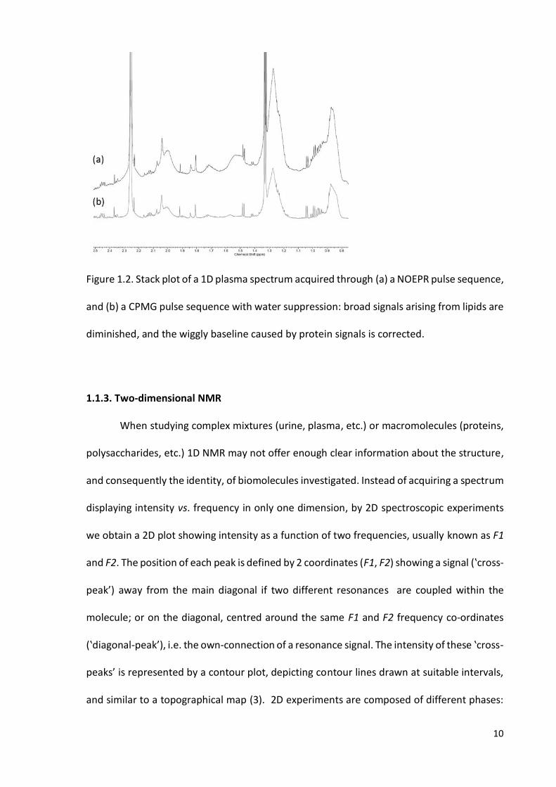
Figure 1.2. Stack plot of a 1D plasma spectrum acquired through (a) a NOEPR pulse sequence,
and (b) a CPMG pulse sequence with water suppression: broad signals arising from lipids are
diminished, and the wiggly baseline caused by protein signals is corrected.
1.1.3. Two-dimensional NMR
When studying complex mixtures (urine, plasma, etc.) or macromolecules (proteins,
polysaccharides, etc.) 1D NMR may not offer enough clear information about the structure,
and consequently the identity, of biomolecules investigated. Instead of acquiring a spectrum
displaying intensity vs. frequency in only one dimension, by 2D spectroscopic experiments
we obtain a 2D plot showing intensity as a function of two frequencies, usually known as F1
and F2. The position of each peak is defined by 2 coordinates (F1, F2) showing a signal (‛cross-
peak’) away from the main diagonal if two different resonances are coupled within the
molecule; or on the diagonal, centred around the same F1 and F2 frequency co-ordinates
(‛diagonal-peak’), i.e. the own-connection of a resonance signal. The intensity of these ‛cross-
peaks’ is represented by a contour plot, depicting contour lines drawn at suitable intervals,
and similar to a topographical map (3). 2D experiments are composed of different phases:
11
preparation, evolution (t1, indirect detection of an additional dimension), mixing
(transference of coherence amongst spins), and detection (t2).
COrrelation SpectroscopY (COSY): This 2D NMR technique shows how proton-
containing functions within molecules are connected to each other in spectra (16). These
experiments are applied to identify molecules through the study of 1H-1H couplings arising
from their structure. In this type of experiment, magnetization is transferred by scalar
coupling. Protons that are more than three chemical bonds away do not generate cross
peaks because the 4J coupling constants are very close to 0. Therefore, only signals of protons
which are two or three bonds apart are visible in a COSY spectrum.
The common pulse sequence is 90ox - t1 - 90o
x - t2, where t1 is the evolution phase and
t2 the detection one. After the first pulse, in a two proton coupling system (A, X), four
different vectors will rotate along the x,y-plane, each of those with a different frequency,
and consequently, fanning out at different velocities from the y-axis. Then, the second pulse
rotates the y component vectors to the -z-axis (which is not detected) and maintains the x
component. Associated with this step, there is transference of magnetization determined by
the spin system situation at t1, which depends in turn on the Larmor frequencies of each
proton A (νA) and X (νX). The x-components of magnetization vectors give an FID, which after
FT with respect to t2 gives a 4 line spectrum containing signals at the frequencies: A1, νA + ½
J (A, X); A2, νA - ½ J (A, X); X1, νX + ½ J (A, X) and X2, νX - ½ J (A, X), which in turn are associated
with the transitions depicted in Figure 1.3. The second FT along t1 yields the 2D spectrum
with 4 groups of 4 signals, two centred around νA, νA and νX, νX (diagonal peaks), and 2 around
νA, νX and νX, νA (cross-peaks) (17). t1 is sequentially-incremented from 0 in Δ intervals, giving

12
for each value for t1 an FID acquired at t2, so that a matrix is composed of rows containing t2
data for t1 = 0 in the first row, with the second row containing t2 data for t1 = Δ, etc. This
whole process is repeated until sufficient data is acquired, typically 50 to 500 increments of
t1 (3).
Figure 1.3. Energy levels scheme and transitions for a two spin AX system conformed for two
1H nuclei.
TOtal Correlation SpectroscopY (TOCSY): In a TOCSY experiment (18, 19)
magnetization is transferred over a complete spin system within the molecule by successive
scalar couplings. The TOCSY experiment involves all protons of a spin system, even if they
are not directly connected.
This experiment is similar to the COSY technique, but in this case we can observe the
whole coupling system, and the second 90o pulse is substituted for a spin-lock stage (90o - t1
- spin-lock - FID) which is equivalent to the mixing period. This stage consists of a low energy
pulse or a series of short pulses in the y-axis direction that locks the My. In order to lock all
the nuclei with regard to their difference Larmor frequencies defined by their nuclear
environments, the spin lock pulse must be tuned in strength and duration. Moreover, the
mixing time (tm) is directly correlated to the spin-system observation; the longer the tm, the
further the whole spin system is extended. The goal of the spin lock stage is to reduce the

13
chemical shift differences (spin locking field << B0), and therefore, those arising from the
scalar coupling will dominate the process (17). This is ascribable to the much lower energy
of B1 when expressed relative to B0. In order to achieve the transference of energy between
nuclei, the Hartman-Hahn condition (20) is required to be accomplished, i.e. different sets of
nuclei all precessing at the same frequency (ν) in order to allow the transfer of energy (cross
polarisation), a condition which is relatively easier to reach in homonuclear systems since all
nuclei have the same γ value (21). The spin-locking field guides the relaxation across My,
yielding a new relaxation time T1ρ, which differs from T1 and T2, but is very similar to T2 when
T1 ≈ T2.
Heteronuclear Single Quantum Coherence (HSQC): This experiment reveals the
connections through a direct bond between 1H and a heteronucleus (i.e., one which differs
from 1H), particularly 13C in a metabolomics context, as cross-peaks in a 2D spectrum. This
experiment was first described by Bodenhausen and Ruben in 1980 (22), who investigated
15N NMR spectra. The pulse sequence is depicted below:
(1H) 90ox - τ - 180o
x - τ - 90oy - t1/2 - 180o
y - t1/2 - 90ox - τ - 180o
x - τ - FID
(13C) τ - 180oy - τ - 90o
x - t1 - 90ox - τ - 180o
x - τ - Decouple
The first part of the pulse sequence (preparation) is the same as INEPT (Insensitive
Nuclei Enhanced by Polarization Transfer), an experiment employed to enhance the intensity
of 13C resonances through the transfer of polarization from directly attached 1H. Then the
system evolves over t1, which is changed incrementally, and finally the 13C polarization is
Detection Mixing Evolution Preparation

14
transferred back to 1H by a reverse INEPT, and its resonance signal subsequently recorded
(17). Polarization transfer occurs when the excitation of one transition of a nucleus modifies
the overall spin population distribution.
Initially, 1H nuclei are flipped towards the y-axis, and then those coupled to either Cα
or Cβ start rotating about this axis at different frequencies during a time τ. After the 180ox
pulse, both vectors (MHCα and MH
Cβ) are oriented oppositely, i.e., about -y-axis. If the system
is left to freely evolve, then an echo would be formed along -y, as noted above, but since
180ox is also applied in the 13C channel, the populations of both levels are inverted, and move
towards the -x and x-axis in the opposite directions from which they started, generating a
180o angle between MHCα and MH
Cβ after τ. Subsequently, the 90oy pulse places the vectors
along -z and z-axis, with MHCβ in the starting position (z-axis) again, and MH
Cα facing the
opposite one (-z-axis) aligned with MC. The 90ox to 13C permits polarization transfer from
proton to carbon. After these 90o pulses, the preparation period ends. MCHβ and MC
Hα start
refocusing on the x-axis to form an echo for a t1/2 period, although the 180ox applied to the
adjacent proton inverts proton magnetization along z-axis where they were residing, and
consequently MCHβ and MC
Hα start fanning out for another t1/2 time, until they form a 180o
angle (antiphase) along the y-axis. This procedure is repeated many times with different t1
increments in order to permit the acquisition of the indirect dimension during this evolution
time. After t1, with the two 90ox pulses in both the 13C and 1H channel, the transfer back of
polarization from 13C to the 1H nucleus is achieved. At this point, transverse magnetization is
attributable to the evolution of protons according to heteronuclear coupling, and therefore
this mixing period corresponds to a reverse INEPT. Subsequent 180ox pulses interchange the
vectors for MHCα and MH
Cβ until they are phased, for both MCHβ and MC
Hα. This last phase
allows observation of the frequency of the more insensitive 13C nucleus as 1H magnetisation.

15
The resulting spectrum shows the 1H resonances on F1, and the 13C ones on F2, and
as both spectra are different, there are not diagonal peaks; only cross-peaks reveal direct
connections between 1H and 13C.
1.2. METABOLOMICS
Metabolomics is the systematic study of the unique ‛chemical fingerprints’ arising
from specific cellular processes, diseases, environmental conditions, mutations, etc. It has
been defined as ‛the quantitative measurement of the multi-parametric metabolic response
of living systems to pathophysiological stimuli or genetic modification’ (23).
The metabolic connections amongst these cellular processes, and particular biofluid
profiles arising therefrom have been noted since the beginning of Medicine as a discipline,
in addition to the possibility of extracting valuable information regarding a disease and/or
its status.
The colour, smell, and taste of urine, for example, were used as diagnostics from
ancient China and India, where clinicians began using ants to detect the sugar content in
urine, as well as tasting it (24). In Greece, since 450 BC Hippocrates developed the theory
that the physical state of a person was correlated with the excess or lack of his/her body
fluids. Galen (AD 131–200) continued with the theory that the health or temperament of a
person was conditioned by the state of the 4 humours: black bile, yellow bile, phlegm and
blood (25). This theory remained until nearly the 18th century. In that age, doctors tended
to purge, bleed or apply pro-emetic techniques in order to equilibrate patient humours and
heal them. In the middle ages, urine was used as a biofluid with a great value in diagnosis
through its smell, taste and colour (Figure 1.4) (26).

16
Figure 1.4. 16th Century diagnostic urine wheel: this urine wheel was published in 1506 by
Ullrich Pinder, in his book Epiphanie Medicorum. It describes the possible colours, smells and
tastes of urine, and their use as a diagnostic tools (26).
In the 1940s, Roger Williams working at Texas University, explored the ability of a
simple method, such as paper chromatography, in order to investigate whether a metabolic
profile can be obtained through the analysis of saliva and urine, this work being the first
proposal for the existence of a metabolic pattern derived from biofluid analysis (27). He
demonstrated that the taste thresholds and the excretion patterns of a variety of molecules
presented inter-individual variability (Figure 1.5), but were homogeneous for each individual
(27).
The technological improvements accomplished in the 1960s and 1970s (first
quadrupole GC/MS instrument) allowed investigators to carry out a detailed quantitative
analysis of metabolic profiles. Accordingly, the Horning group in the 1970s demonstrated
how gas chromatography-mass spectrometry (GC-MS) could be employed to investigate a
wide range of compounds present in human urine and tissue extracts; they also created the
17
term ‘metabolic profile’ (28-30). The investigations conducted by the Horning group,
together with that of Linus Pauling and Arthur B. Robinson led to the development of GC-
MS methods to detect and identify metabolites present in urine (31).
Figure 1.5. Polar co-ordinates of the metabolic patterns of 4 subjects studied by R. Williams
in 1940: data were obtained by measurements of taste thresholds (numbers 1-17), and
urinary metabolites (numbers 18-31). The lengths of the lines are indicative of the amounts
of compounds determined (27).
The establishment of metabolic profile determinations in biological samples using
high-resolution NMR analysis provides a detailed and specific view into cellular metabolic
processes under normal and altered (disease-related) conditions. Indeed, continuing the
work performed on GC-MS for biofluid profiling in previous years, McConnell, M. L. et al.
published their work on pattern recognition using this technique (32).

18
In 1974, the NMR analysis of tissue began its development with investigations
conducted by Hoult et al. focused on the 31P NMR analysis of intact biological samples (Figure
1.6). They analysed muscle tissue in order to explore the complexation of ATP with
magnesium (33); this is known to be the first NMR analysis applied to a biopsy. One year
later, an NMR analysis of intact frog muscle was also reported by Bárány and co-workers
(34). Therefore, these studies of organs and tissues by NMR analysis that led to the
development of modern in vivo NMR spectroscopy (35) commenced 40 years ago.
Figure 1.6. Experiment performed by Hoult et al. involving 31P-NMR analysis (129 MHz) of
muscle: intact muscle from the hind leg of a rat. Peak assignments: I, sugar phosphate and
phospholipids; II, inorganic phosphate; III, creatine phosphate; IV, γ-ATP; V, α-ATP; VI, β-ATP
(33).
In the late 1970’s 1H NMR analysis started to be proposed as a non-invasive technique
for the metabolic profiling of biofluids and tissue by D. Rabenstein and co-workers (36, 37).
A few years later, in the middle 1980s, Jeremy Nicholson and Peter Sadler at Birkbeck College
(University of London, UK), and later at Imperial College (London, UK) demonstrated how 1H

19
NMR spectroscopy could be utilised as a valuable diagnostic tool, and applied this technique
to establish a diabetic metabolic profile and subsequently developed the study of NMR
spectroscopy linked to pattern recognition in the mid- to late 1980s (38). This work
performed by Nicholson and co-workers on plasma analysis by 1H NMR was based on the
application of the newly-introduced pulse sequences utilised to supress the broad signals
arising from the macromolecules such as proteins and lipids by Daniels et al. in 1976 (39),
and in the previous investigations conducted by Bock in 1982 (40), in which this author
analysed blood plasma by NMR for the first time, exploring the 1H NMR plasma spectral
change in patients suffering from lactic acidosis, those undergoing phenobarbital treatment,
and also investigating the detection of ethanol resonances in his own plasma profile
following vodka consumption.
In 1985, Arús et al. were the first investigators to assign the 1H NMR resonances in
spectra of excised rat brain (41). In frog, rat and human skeletal muscle, the 1H resonances
found were virtually the same as those detected in rat brain. Furthermore, the =N-CH3
resonance signal of creatine at 3.02 ppm was proposed to be used as internal reference for
chemical shift values (42).
Interestingly, all this early metabolomics research work was devoid of a name to
define the class of research performed, so that the first paper using the word metabolome
was Oliver S. G. et al. (Trends. Biotechnol. 1998. 16:373).
In 2005, the Siudzak group at The Scripps Research Institute (CA, USA) developed the
first Metabolomics web database (METLIN), which contained over 10,000 metabolites and
tandem MS data. On 23th of January of 2007, the Human Metabolome Project, led by David
Wishart (University of Alberta, Canada), completed the first draft of the human metabolome,
and this database primarily contained approximately 2,500 metabolites, 1,200 drugs and

20
3,500 food components (43). An additional database available that contains NMR spectra of
metabolites is the Biological Magnetic Resonance Data Bank (BMRB) run by the University of
Wisconsin, which also hosts spectra from peptides, proteins and nucleic acids (44).
Moreover, the Spectral Database for Organic Compounds (SDBS), created by the National
Institute of Advanced Industrial Science and Technology (Japan) contains not only NMR
spectra, but also MS, Electron Spin Resonance (ESR), Infra-Red (IR) and Raman ones. These
databases have incredibly aided the identification of metabolites, and the information
contained therein has been updated and enlarged with recently published works regarding
the identification and resolution of the majority of resonances present in urinary (45), blood
serum (46) and salivary (47) 1H NMR profiles.
The future of NMR-linked metabolomics is moving towards both the automation of
all the analytical steps performed after spectral acquisition, and also the standardization of
experimental conditions. Accordingly, automated assignment web-based software has been
developed, i.e. COLMAR (48), and software developed by the Wishart group allows the
automatic resonance signal deconvolution for quantitative Metabolomics, BAYESIL (49). The
next step in a metabolomics investigation after the completion of all resonance assignments
is multivariate analysis, and this can be performed by the web-based tool MetaboAnalyst 3.0
(50) that allows researchers to analyse datasets through a wide battery of multivariate and
univariate analysis techniques, and also includes modules for time-series and pathway
analyses. The standardization of NMR-linked Metabolomics investigations is a major concern
for the scientific community, mainly in the field of urine NMR analysis as a diagnostic tool
(51), since plasma analysis investigations are still being subjected to new developments, both
in terms of signals assignments [mainly lipoprotein subclass identification (52)] and the
dichotomy between physically (ultrafiltration, organic solvent precipitation) (53) or NMR-

21
based suppression of the broad signals attributable to macromolecules present in this
biofluid. Nevertheless, Nicholson and co-workers have reported a set of protocols for human
urine, serum, and plasma NMR-linked metabolomics analysis in order to provide
standardized steps in metabolomics investigations (54). This effort for standardizing the
experimental procedures in NMR-linked urinary metabolomics analysis includes all the steps
involved in such investigations, from sample collection and preparation to the manner in
which investigators should report their results (55). In order to accomplish this ambitious
objective, the Metabolomics Society released the Metabolomics Standards Initiative in 2007
(56). In 2012, a further initiative known as the coordination of standards in metabolomics
(COSMOS) was set up to bring together metabolomics researchers to develop guidelines and
standard workflows for metabolomics applications (www.cosmosfp7.eu). Additionally, the
standardization of urinary metabolite quantification serves as a further step, since it would
translate the investigations from laboratory to clinic, since proposing metabolites as
biomarkers irremediably requires the provision of accurate threshold metabolite values in
order to distinguish healthy from diseased patients in a diagnostic test (57).
In the NMR-linked metabolomics field, the major instrumental advances are driven
towards a decrease in the spectral acquisition duration for homo- and heteronuclear 2D
spectroscopy in order to facilitate the assignment of resonances within reduced time
periods. Throughout the last five years, the development of ultrafast NMR experiments has
allowed the acquisition of 2D NMR spectra in a single scan (58), which may permit the
development of high-throughput 2D NMR-based metabolomics studies (59). Moreover, Rai
and Sinha (2012) reported a new J-compensated HSQC pulse sequence which reduces the
data collection time 22 times, and which does not show any deficiency in the quantification
of low abundance metabolites (60).

22
1.3. MULTIVARIATE STATISTICAL ANALYSIS TECHNIQUES
1.3.1. Principal Component Analysis (PCA)
The PCA technique is attributable to Hotelling (61), although its origins are in the
orthogonal least-squares adjustments introduced by K. Pearson, who first proposed it over
100 years ago (62). By applying PCA, we seek to maximize the percentage of variance
explained using linear combinations of ‛predictor’ variables, the so-called components. PCA
is an unsupervised technique, since these components are selected without any assumption
about the group classification and hence clusterings that might underlie the dataset;
therefore, no grouping of observations is assumed. The information lies in the correlation
structure, and both clustering tendency and outliers can be detected.
A dataset with K-variables can be geometrically represented by a plane of K-
dimensions. The goal of PCA is to reduce the number of dimensions, together with an
explanation, with those few dimensions, of the maximum variation of the dataset (Figure
1.7).
Each sample/observation is represented in the PCA space as a point with K-
coordinates. The samples in that space have to be centred first, by subtracting the mean,
and PCA then draws a line through the K-dimensions that best approximate the data
(ordinary least squares technique), which would represent the first component. It is usually
convenient to standardize the variables prior to principal component analysis computations,
since those variables which present a higher contribution towards the total variance
dominate computation of the first PC. This first PC is obtained as a linear combination of the
variables with the aim of achieving maximal variance; then, the second PC is obtained as a
linear combination of the original variables, with the same purpose of achieving maximal
variance, in an orthogonal direction to the first PC, and so on (63).
23
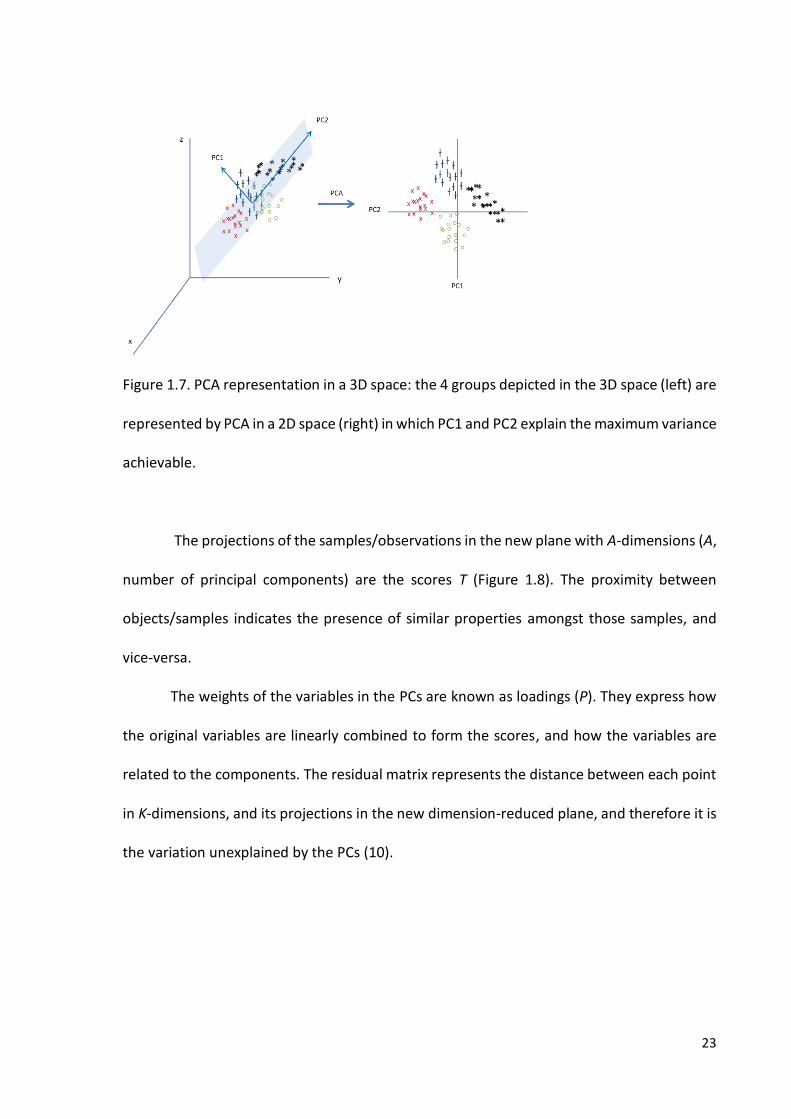
Figure 1.7. PCA representation in a 3D space: the 4 groups depicted in the 3D space (left) are
represented by PCA in a 2D space (right) in which PC1 and PC2 explain the maximum variance
achievable.
The projections of the samples/observations in the new plane with A-dimensions (A,
number of principal components) are the scores T (Figure 1.8). The proximity between
objects/samples indicates the presence of similar properties amongst those samples, and
vice-versa.
The weights of the variables in the PCs are known as loadings (P). They express how
the original variables are linearly combined to form the scores, and how the variables are
related to the components. The residual matrix represents the distance between each point
in K-dimensions, and its projections in the new dimension-reduced plane, and therefore it is
the variation unexplained by the PCs (10).

24
Figure 1.8: Matrix representation of a PCA model: X, original dataset; P, loadings matrix; T,
scores matrix; E, residual matrix.
In some situations, loadings of some variables might have medium correlation values
to the factors, which may lead to a difficult interpretation of the results. In order to facilitate
this interpretation, the factors can be rotated to make the correlations of the variables to
the factors more polarized. Rotation can be either orthogonal or oblique, the former being
the most widely employed since the factors arising from the components’ rotation remain
orthogonal, as are the PCs from which they are generated. Through a rotation of the
components [linear combination of the original factors such that the variance of the squared
loadings is maximized (64)], the explained variance changes from the PCs to the new
rotation-derived factors, but the total amount of explained variance remains the same, i.e.
the only change is the partition of the variance into factors. Varimax (65) is the most widely
used rotation technique, and it attempts to reduce the number of variables with higher
loadings within a factor, and also the number of variables associated with several factors
simultaneously (64).
1.3.2. Linear Discriminant Analysis (LDA)
Linear discriminant analysis (LDA) is a statistical method which seeks a linear
combination of the variables in order to achieve the best discrimination between the initial

25
groups investigated (66). Moreover, it can be employed to define decision rules in order to
classify a new sample, the class of which is unknown.
This method finds the linear combination of the features that maximizes the ratio of
‛between-class’ variance to the ‛within-class’ variance in any particular dataset, thereby
guaranteeing maximal separation (67).
If the dataset is represented by the matrix X = (x1, x2,…xn), where n is the number of
observations, xi being an observation described by q features, then μk is the mean of a class
Ck and μ is the overall mean of all the observations:
𝑆𝐵 = ∑ (μ𝑘 − μ)(μ𝑘 − μ)𝑡𝑘 (5)
𝑆𝑤 = ∑ ∑ (μ𝑖 − μ)(μ𝑖 − μ)𝑡𝑥𝑖𝜖𝐶𝑘𝑘 (6)
SB and SW represent the ‛between-class’ and ‛within-class’ scatter matrices
respectively. The sum of both gives the covariance matrix for the whole dataset.
The aim is to seek and find a projection of the dataset, in the d dimensional plane,
where it achieves a maximum separation between the mean values of projected classes, and
minimum variance within each projected class so that wtSB w is maximized and wtSW w is
minimized. This dual objective can be reached through the vector wopt, which attemps to
maximize the following function:
𝐽(𝑤) = 𝑤𝑡𝑆𝑏𝑤
𝑤𝑡𝑆𝑤𝑤 (7)
This LDA approach is similar to PCA, but in this case we not only seek to find the
components that maximize the variance, but additionally, we attempt to achieve a maximal
26
separation between classes, differentiating between variability ‛between-groups’ (SB) and
‛within-groups’ (SW). If the structure underlying the dataset reveals that SB >>> SW, then PCA
also performs well for classification purposes.
1.3.3. Partial Redundancy Analysis (pRDA)
RDA is a technique that combines regression and PCA in order to model multivariate
response data (68). Indeed, RDA (69) with a single ‛response’ variable is equivalent to
multiple linear regression modelling. The operation of this method can be viewed as a
multivariate linear regression of Y (response variables matrix, n x p) on X (explanatory
variables matrix, n x m), yielding a matrix of fitted values, known as �̂�. Subsequently, a PCA
on �̂� is performed in order to obtain a matrix of the canonical axes (similar to the scores
matrix in a PCA).
Permutation tests are usually employed to check if the linear combinations of X are
truly explaining Y, and consequently the R2 value, a parameter that represents how well a
model fits the original data (with a score of 0 indicating an absolute lack of fitting, and 1.00
a perfect fitting of the data), together with the p-value obtained when the observed case is
tested against those obtained after randomly permuting the yi variables within the Y matrix,
perhaps several thousand or more times.
Partial Redundancy Analysis (pRDA) is method first proposed by Davies & Tso in 1982
(70), in which an additional matrix of covariables W, influences the response variables Y. This
approach is applied to control the known effects of a covariable, when analysing the effect
of a set of variables X on Y (71). Another application of this model is to isolate the effect of a
single explanatory variable or factor.
27
1.3.4. Correlated Component Regression (CCR)
Correlated Component Regression (CCR) is an ensemble dimension reduction
regression technique that provides reliable predictions even with near multicollinear data
(72). Correlation amongst variables, known as multicollinearity, is a common problem
encountered when dealing with large datasets, and consequently, traditional regression
techniques may estimate unstable coefficients (73). Situations where the number of
predictor variables P approaches or exceeds the sample size N give rise to major problems,
and such instability is often accompanied by perfect or near perfect predictions of the
regression model developed. However, this seemingly good predictive performance is
usually associated with overfitting, and is not accurate when new samples are employed to
test the model (72).
CCR proposes the prediction of the dependent variable based on K correlated
components. If K = 1, CCR is equivalent to the corresponding Naïve Bayes solution
(probabilistic classifier based on the application of Bayes' theorem with independence
assumptions) (74). It is further suggested that for K > 1, CCR represents a natural extension
of a Naïve Bayes model applied to multiple dimensions (74).
Estimation of components: CCR utilizes K < P correlated components in place of the
P predictors to estimate the response variable (75). Each component Sk is an exact linear
combination of the variables, X = (X1, X2,…XP). The first component S1 captures the effects of
those predictors that have direct effects on the outcome (72). Unlike PCA, the objective is
not to explain the correlation/covariance matrix through the weights of the components
(percentage of variance explained), but to compute the weights with the aim of maximizing

28
the ability to predict the outcome (75). The CCR-linear model (CCR-LM) algorithm proceeds
as follows:
Estimate the loading λg(1), on S1, for each predictor g = 1, 2,…P, as the simple
regression coefficient of the regression of Y on Xg . Component S1 captures the direct effects
of X for the regression y on X as a weighted average of the one predictor model.
𝜆𝑔(1)
=𝐶𝑜𝑣 (𝑌,𝑋𝑔)
𝑉𝑎𝑟(𝑋𝑔 ) (8)
𝑆1 = ∑ 𝜆𝑔(1)𝑃
𝑔=1 𝑋𝑔 (9)
The first component S1 is computed as a linear combination of X using 𝜆𝑔(1)
as weights.
Similarly, predictions for the 2-component CCR model are obtained from the simple OLS
regression of Y on S1 and S2. Components are related to each other, and they are not
orthogonal as in other techniques (PCA, Partial Least Squares); this correlation allows the
mutual enhancement of the predictive abilities of the whole set of components, so that S2
improves the performance of predictor S1, S3 improves that for S2, and so forth, with the aim
to achieve the desired effect of removing ‘extraneous variation’.
Component Sk′ for k′ > 1, is defined as a weighted average of all 1-predictor partial
effects, where the partial effect for predictor g is computed as the partial regression
coefficient in the OLS regression of Y on Xg, and also on all previously computed components
Sk,k = 1,… k’ -1 (75).
𝑌 = 𝛼 + 𝛾1.𝑔(2)
𝑆1 + 𝜆𝑔(2)
𝑋𝑔 + 𝜀𝑔(2)
(10)
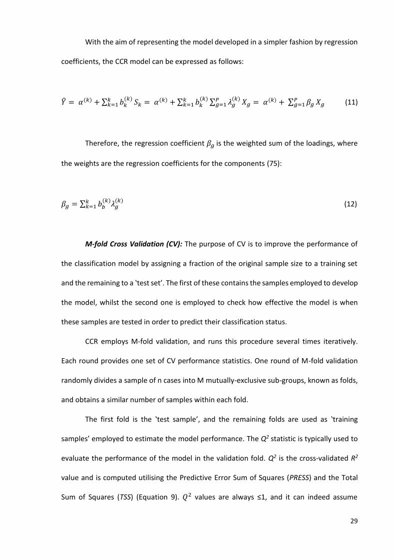
29
With the aim of representing the model developed in a simpler fashion by regression
coefficients, the CCR model can be expressed as follows:
�̂� = 𝛼 (𝑘) + ∑ 𝑏𝑘
(𝑘)𝑘𝑘=1 𝑆𝑘
= 𝛼 (𝑘) + ∑ 𝑏𝑘
(𝑘) ∑ 𝜆𝑔(𝑘)𝑃
𝑔=1 𝑋𝑔 =𝑘
𝑘=1
𝛼
(𝑘) + ∑ 𝛽𝑔 𝑃
𝑔=1 𝑋𝑔 (11)
Therefore, the regression coefficient 𝛽𝑔 is the weighted sum of the loadings, where
the weights are the regression coefficients for the components (75):
𝛽𝑔 = ∑ 𝑏𝑏(𝑘)
𝜆𝑔(𝑘)
𝑘𝑘=1 (12)
M-fold Cross Validation (CV): The purpose of CV is to improve the performance of
the classification model by assigning a fraction of the original sample size to a training set
and the remaining to a ‛test set’. The first of these contains the samples employed to develop
the model, whilst the second one is employed to check how effective the model is when
these samples are tested in order to predict their classification status.
CCR employs M-fold validation, and runs this procedure several times iteratively.
Each round provides one set of CV performance statistics. One round of M-fold validation
randomly divides a sample of n cases into M mutually-exclusive sub-groups, known as folds,
and obtains a similar number of samples within each fold.
The first fold is the ‛test sample’, and the remaining folds are used as ‛training
samples’ employed to estimate the model performance. The Q2 statistic is typically used to
evaluate the performance of the model in the validation fold. Q2 is the cross-validated R2
value and is computed utilising the Predictive Error Sum of Squares (PRESS) and the Total
Sum of Squares (TSS) (Equation 9). 𝑄2 values are always ≤1, and it can indeed assume

30
negative values when PRESS > TSS, revealing that the model performs worse when it is
evaluated with the ‛test set’ than the mean response of the ‛training set’ (76):
𝑄2 = 1 − 𝑃𝑅𝐸𝑆𝑆
𝑇𝑆𝑆= 1 −
∑ (𝑦𝑖− 𝑦�̂�)2𝑛𝑖=1
∑ (𝑦𝑖− �̅�)2𝑛𝑖=1
(13)
This result on fold 1 is then stored, and the process is repeated for the second fold.
The model’s predictive performance is then tested on this 2nd validation fold, and the results
aggregated with the previous CV performance (from fold 1). The process is then repeated
for the remaining folds.
Step-Down Procedure: This approach works in conjunction with M-fold cross-
validation. For a particular value of K (number of correlated components), a model with all
possible predictors is initially estimated. Subsequently, the least important predictors are
left out based on their standardised effect (Equation 14), and the Q2 value for the new model
is obtained using the original set of predictors minus the ‛worst’ (75). This process then
repeats until we have Q2 values for every possible model (75).
𝛽𝑔∗ = (
𝜎𝑔
𝜎𝑦 ) 𝛽𝑔
(14)
CCR uses a step-down variable selection algorithm in order to remove irrelevant
predictors, which commences using all the variables for developing the model; subsequently,
it eliminates those variables with the smallest standardised coefficients one by one, re-
estimating the model at each step (72).
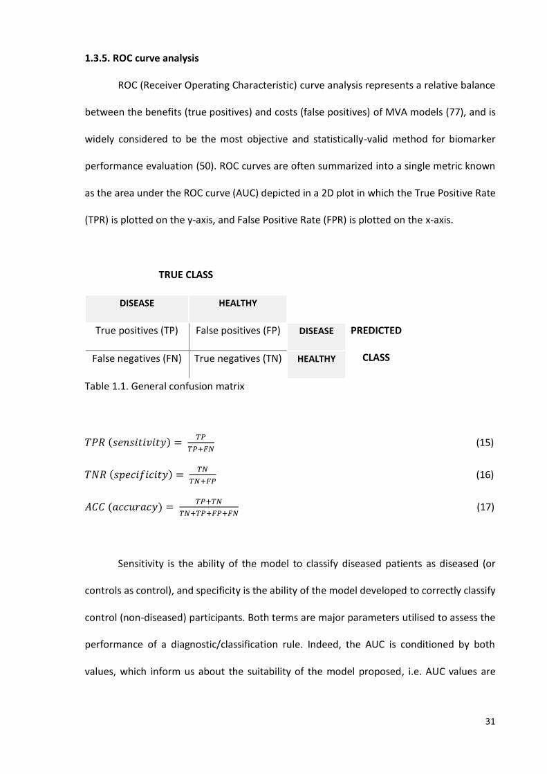
31
1.3.5. ROC curve analysis
ROC (Receiver Operating Characteristic) curve analysis represents a relative balance
between the benefits (true positives) and costs (false positives) of MVA models (77), and is
widely considered to be the most objective and statistically-valid method for biomarker
performance evaluation (50). ROC curves are often summarized into a single metric known
as the area under the ROC curve (AUC) depicted in a 2D plot in which the True Positive Rate
(TPR) is plotted on the y-axis, and False Positive Rate (FPR) is plotted on the x-axis.
TRUE CLASS
DISEASE HEALTHY
True positives (TP) False positives (FP) DISEASE PREDICTED
CLASS False negatives (FN) True negatives (TN) HEALTHY
Table 1.1. General confusion matrix
𝑇𝑃𝑅 (𝑠𝑒𝑛𝑠𝑖𝑡𝑖𝑣𝑖𝑡𝑦) = 𝑇𝑃
𝑇𝑃+𝐹𝑁 (15)
𝑇𝑁𝑅 (𝑠𝑝𝑒𝑐𝑖𝑓𝑖𝑐𝑖𝑡𝑦) = 𝑇𝑁
𝑇𝑁+𝐹𝑃 (16)
𝐴𝐶𝐶 (𝑎𝑐𝑐𝑢𝑟𝑎𝑐𝑦) = 𝑇𝑃+𝑇𝑁
𝑇𝑁+𝑇𝑃+𝐹𝑃+𝐹𝑁 (17)
Sensitivity is the ability of the model to classify diseased patients as diseased (or
controls as control), and specificity is the ability of the model developed to correctly classify
control (non-diseased) participants. Both terms are major parameters utilised to assess the
performance of a diagnostic/classification rule. Indeed, the AUC is conditioned by both
values, which inform us about the suitability of the model proposed, i.e. AUC values are

32
considered excellent if they lie between 0.90 - 1.00, good for 0.80 - 0.90, fair for 0.70 - 0.80,
poor for 0.60 - 0.70 and of no value for ≤0.6) (78).
1.4. ARTIFICIAL INTELLIGENCE BASED TECHNIQUES
1.4.1. Random Forests (RFs)
Random Forests is a prediction/classification model technique consisting of an
ensemble of classification and regression tree-structured classifiers (79).
Decision trees are classifiers which use a single feature at each non-terminal node,
so that a sample is classified to the left or the right branch at that specific node if its value
for that feature is greater or less than the threshold specified at that node. At each split, the
data is partitioned in two mutually-exclusive groups, and attempts to achieve as much
homogeneity as possible in each group; subsequently, the splitting is repeated for each
group in order to improve this homogeneity within them, but with the constraint of having
a tree relatively small and easy to interpret (80). Once the tree is unable to continue the
splitting of samples into different groups, the process completes. The tree can then be
‛pruned’ back to the desired size.
In 1984, Brieman, Olshen, Friedman and Stone published the book ‛Classification and
Regression Trees’, and developed the CART software (81). This book presented the
applicability of RFs and its successful performance when attempting to solve a range of
problems that one of the researchers faced when he was working at the UC San Diego
Medical School.
RFs uses an ensemble of classification trees; each of these trees is grown by random
feature selection from a ‛bootstrap’ sample [‛training set’ sub-samples with replacements

33
obtained from the original dataset (82)] at each branch (83). Class prediction is based on the
average classification performance of the aggregate of trees. The process of building up a
tree consists of selecting a bootstrap sample of 63.2% (on average) from the original whole
sample set, and then a random group of variables are chosen for splitting at a particular
node. The remaining 36.8% sub-set is then employed to obtain an unbiased estimate of the
classification error (out-of-bag error, OOBE error) (84). Since the OOB observations are not
used for fitting the trees, this is a cross-validated accuracy estimate, and hence it represents
an unbiased estimation of the generalization error (79). Variable importance is evaluated via
measurements of the increase of the OOB error value when it is permuted (79). The OOB
error estimate ranges from 0 (if the model is able to predict with a 100% in accuracy the class
of the test set) to a value of 1.00 (no sample from the test set was correctly classified).
1.4.2. Support Vector Machines (SVMs)
Support Vector Machines were originally developed in 1982 by Vapnik (85), and the
most relevant outcome appeared in 1992 with the seminal Boser, Guyon and Vapnik paper:
‛A training algorithm for optimal margin classifiers’, in which this technique was formally
proposed (86).
SVMs is a classification algorithm that operates by finding the decision surface that
can more clearly separate samples from different classes, and hence has the largest distance
between borderline samples (support vectors). Separation is then achieved by identifying
these support vectors for the respective classes, identifying the separating hyperplane (space
of K-1 dimensions constructed in a K-dimensional space, where K > 3) in between, so that
these points are the most influential ones over the parameters selected to ‛draw’ this
hyperplane in such a manner that moving a support vector moves the hyperplane. However,

34
the remaining samples do not have any influence in the process of seeking of this
hyperplane. Therefore, the algorithm generates the weights, and only considers the support
vectors to define their values, and hence the boundary. Nevertheless, if this decision surface
does not exist, then the dataset has to be mapped onto a higher dimensional space where
this decision surface exists. This transformation is known as the Kernel trick.
If the training set xi ∈ Rn, i= 1... m where each of the xi (samples) belong to one of the
two categories yi, indicated by either -1 or 1, SVMs finds a hyperplane with the parameters
(w,b), using the following convex optimization problem to obtain them (86):
min𝑤,𝑏,𝜖
1
2𝑤𝑡𝑤 + 𝑐 ∑ 𝜖𝑖
𝑁𝑖=1 (18)
subject to 𝑦𝑖(𝑤𝑡𝑥𝑖 + 𝑏) ≥ 1 − 𝜖𝑖 , where 𝜖𝑖 ≥ 1, for i = 1,…N
In Equation 18, c works as a regularization parameter which acts as a ‛slack’ constant,
and which is a ‛trade-off’ between the ability of the system to model accurately using the
training set, and its predictive performance (87). If c is small, then the margin is large, so
constraints are easily ignored; however, if c is large, then the margin is narrow, and therefore
constraints are hard to ignore, so that c controls the margin width. 𝜖𝑖 is a measure of
misclassification rate and is also known as the ‛slack variable’. The function of this term is to
reduce the overfitting problem, enhancing the performance of SVMs, but also allowing a
fraction of training sample objects to be within the margin or even misclassified in order to
not introduce more complexity within the model (i.e., a ‛soft’ margin classifier).
35
1.4.3. Genetic Algorithms (GAs)
GAs are randomized search and optimization algorithms inspired by Darwin’s theory
of evolution that were introduced by Holland in 1975 (88). GAs function as a simulation of
an evolutionary process, in which a population of solutions evolve over a sequence of
generations (89) (Figure 1.9). Each chromosome represents a potential solution, and the
fitness value associated with each chromosome indicates its relevance to obtain the best
possible solution (90).
Encoding and Initial Population: A chromosome is a string of ‘bits’ with a length
determined by the total number of variables. The presence/absence of a variable in the
chromosome is given by the value 1 or 0 in the corresponding i-th place within the
chromosome; this assignment is generated randomly. Consequently, each chromosome
represents a different sub-set of features.
Selection, Crossover and Mutation: The selection process involves the principle of
‛Survival of the fittest’, i.e. improved solutions are selected to get through to the next
generation; notwithstanding, ‛bad’ solutions are discarded. The ‛good & bad’ criteria are
given by the fitness function.
Crossover causes a structured yet randomized exchange of genetic information
amongst solutions/chromosomes, with the aim that effective solutions could be crossed with
other high-performance ones in order to generate improved models. This process is applied
with a probability, called crossover rate, i.e. the probability that a chromosome (solution)
experiences cross-over during its reproduction process. A crossover rate of 1.00 indicates
that all the chromosomes experience crossover, so no unchanged solutions go through to
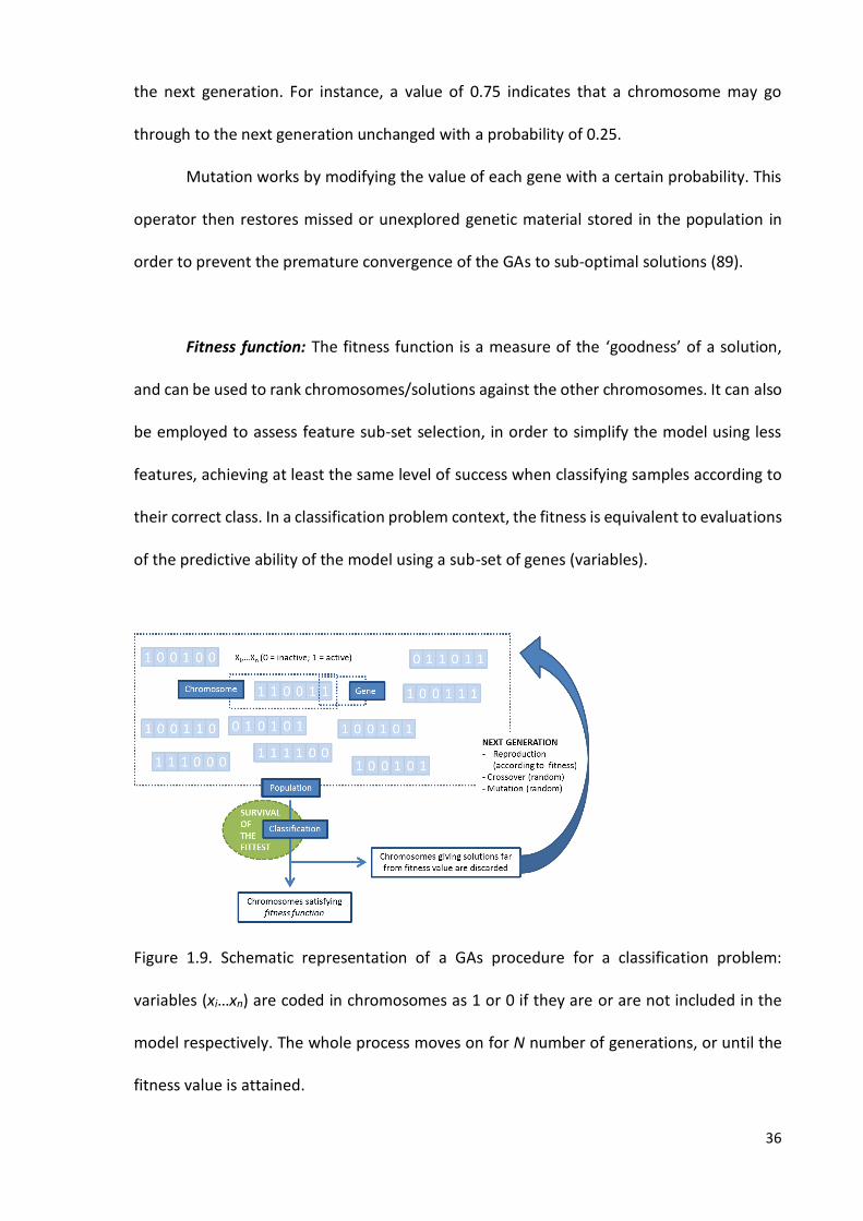
36
the next generation. For instance, a value of 0.75 indicates that a chromosome may go
through to the next generation unchanged with a probability of 0.25.
Mutation works by modifying the value of each gene with a certain probability. This
operator then restores missed or unexplored genetic material stored in the population in
order to prevent the premature convergence of the GAs to sub-optimal solutions (89).
Fitness function: The fitness function is a measure of the ‘goodness’ of a solution,
and can be used to rank chromosomes/solutions against the other chromosomes. It can also
be employed to assess feature sub-set selection, in order to simplify the model using less
features, achieving at least the same level of success when classifying samples according to
their correct class. In a classification problem context, the fitness is equivalent to evaluations
of the predictive ability of the model using a sub-set of genes (variables).
Figure 1.9. Schematic representation of a GAs procedure for a classification problem:
variables (xi…xn) are coded in chromosomes as 1 or 0 if they are or are not included in the
model respectively. The whole process moves on for N number of generations, or until the
fitness value is attained.
37
1.5. NIEMANN PICK TYPE C1 DISEASE
1.5.1. Description
Niemann-Pick type C (NP-C) disease is a neurodegenerative lysosomal storage
disorder caused by mutations in the NPC1 and NPC2 genes, the hereditability of which is
autosomic recessive (91). Approximately 95% of patients have mutations in the NPC1 gene
(mapped at 18q11) which encodes a large membrane glycoprotein located in late
endosomes (92) . The remaining 5% have mutations in the NPC2 gene (mapped at 14q24.3)
which encodes a small soluble lysosomal protein that binds cholesterol in the lumen of this
organelle (92). Patients with NP-C1 and NP-C2 diseases are indistinguishable, both clinically
and in terms of the standard biochemical tests for NP-C diagnosis (93).
In 1984, Pentchev and colleagues made the highly significant discovery that the
major biochemical feature of NP-C disease is lysosomal accumulation of LDL-derived,
unesterified (free) cholesterol, and consequently, these patients develop a dysregulated
sterol biosynthesis, uptake and esterification (94). The estimated incidence of the disease is
approximately 1:120,000 live births, based on studies performed during the past 20 years
(95).
1.5.2. Cell biology of cholesterol
Cholesterol, which is the major steroid present in animal tissues, stabilizes the
structure of plasma membranes, regulates membrane permeability, and reinforces the liquid
ordered phase of lipid bilayers (96). It is essential for myelin formation (97), and during
development it has a major signalling pathway function, specifically in the hedgehog
signalling pathway, in which cholesterol covalently modifies the proteins involved in order

38
to render them functional (98, 99). Cholesterol binds to the amino terminal peptide arising
from the autoproteolitic cleavage of the original protein (i.e. those involved in the hedgehog
pathway), and it is only this N-terminal peptide which has signalling activity, involved for
example in skeletal (100) and cerebellum development (101). Cholesterol is a precursor of
corticosteroids, vitamin D, bile acids and steroid hormones.
Not all mammalian cells are able to metabolize cholesterol. In fact, only liver and
steroidogenic tissues do. Nevertheless, other tissues unable to metabolize this molecule are
capable of modulating its concentration in the membranes by regulating the biosynthesis,
uptake, and export of cholesterol from the cell through ATP-binding cassette (ABC)
transporters (102).
Cholesterol can be obtained by cells through two routes. Firstly, it can be acquired
from the diet associated with plasma low-density-lipoproteins (LDLs), in which cholesterol
from the liver can be transported through the circulation to extra-hepatic tissues, being
initially packaged in very-low-density-lipoproteins (VLDLs). In the circulation, VLDLs are
converted to LDLs by the action of lipoprotein lipase.
LDLs are taken up by cells via LDL receptor-mediated endocytosis. The interaction of
LDLs with LDL receptors requires the presence of apoB-100, the exclusive apolipoprotein of
LDLs. The endocytosed vesicles (endosomes), derived from the internalization of the
membrane, then fuse with lysosomes, where the apoproteins (originally contained in LDLs),
are degraded; subsequently, cholesteryl esters are hydrolysed within the lysosome yielding
free cholesterol. This cholesterol moiety is then incorporated into the plasma membranes
where required, predominantly at the cytoplasmic membrane, where LDL-cholesterol
released from lysosomes can be rapidly detected (103). The caveolae (special region within
the membrane which is rich in cholesterol and sphingomyelin) are the first destination for
39
the free cholesterol carried by LDL. However, to elicit homeostatic responses and to be
transformed to cholesteryl esters and bile acids, or indeed incorporated into lipoproteins,
cholesterol must first reach the endoplasmic reticulum (ER) (103).
Alternatively, cholesterol can be generated via de novo synthesis in the endoplasmic
reticulum. LDLs are not able to go through the blood-brain barrier (BBB) and supply the brain;
furthermore, this de novo pathway is the only and exclusive mechanism for the central
nervous system (CNS) to obtain cholesterol. Free cholesterol synthesised in the glia and
complexed with apolipoprotein E is then delivered to neurons (104). Although LDL cannot
cross the BBB, cholesterol can egress from the CNS as 24-hydroxy-cholesterol. Furthermore,
27-hydroxy-cholesterol can also cross the BBB in the opposite direction (105).
1.5.3. NPC1 and NPC2 proteins
The multivesicular late endosomes accommodate two proteins, NPC1 and NPC2,
which are crucial for moving cholesterol out from the endosomal system (Figure 1.10).
Therefore, deficiencies in the levels or activity of these proteins lead to the accumulation of
LDL-derived unesterified cholesterol in LE (106).
In NP-C disease, the movement of LDL-derived cholesterol to the endoplasmic
reticulum and plasma membrane is delayed, resulting in altered regulation of cholesterol
homeostasis in the ER. Hence, cholesterol and LDL-receptor synthesis is enhanced to
compensate for the apparent lack of cholesterol detected by the cell; additionally,
cholesterol esterification is diminished (107). In contrast, intracellular transport of
cholesterol delivered from exogenously-supplied high-density-lipoproteins (HDLs) seems to
be unaffected in the disease, and this is presumably ascribable to this source of cholesterol
not entering late endosome/lysosome via endocytosis (107).

40
Figure 1.10. Potential mechanism for NPC1/NPC2-mediated cholesterol export from late
endosome/lysosome: CE, cholesteryl ester; FA, unesterified fatty acid; LBPA/BMP, lyso-bis
phosphatidic acid, also known as bis-(monoacylglycerol)phosphate (108). NPC2 (soluble
protein) binds unesterified cholesterol in the late endosome/lysosome with the iso-octyl
chain in the binding pocket, an event that may be enhanced by bis-
(monoacylglycero)phosphate. NPC2 transfers cholesterol to the N-terminal loop of NPC1 (a
multi-pass membrane protein) which binds cholesterol, accommodating the hydroxyl group
in the binding pocket. Cholesterol is exported from late endosome/lysosome by an unknown
mechanism (109). [Figure taken from (108)]
Other biomolecules are also stored within the lysosome in this disease, including
complex gangliosides such as GM1 and GM2, glucosyl and galactosylcerebrosides (108). NPC1
and NPC2 proteins have been proposed to be involved in the endosomal/lysosomal
processing of these lipids, since simple gangliosides (e.g. GM2, GM3) can be delivered to Golgi
after being endocytosed by the late endosome/lysosome system to generate more complex

41
structures as an alternative to the de novo synthesis pathway (110). Therefore, mutated
NPC1 and/or NPC2 lead to the accumulation of these gangliosides.
A sequential process of pathological effects derived from NPC1 gene
mutation/inactivation has been recently proposed, in which the first consequence of this
genetic alteration is sphingosine storage, folllowed by deficient calcium homeostasis within
the lysosome which leads to a reduced calcium release and consequently a block in late
endosome/lysosome fusion that finally causes unsterified cholesterol storage (111).
Accordingly, the storage of cholesterol, which was previously thought to be the main
activator of the molecular disease process, is actually the trigger of all the neurodegenerative
processes that subsequently occur.
1.5.4. Disease manifestations
The manifestation of NP-C1 disease is very heterogeneous, and actually it can vary
between siblings (95), which leads a delay in in diagnosis of 5–6 years from the onset of
neurological symptoms (112, 113). Therefore, the individual features illustrated in Figure
1.11 are not NP-C1-specific, but the conjunction of all of them generates a clinical picture
which is considered disease-specific.
Neurological features include abnormal saccadic eye movements, ataxia, dystonia,
dysarthria and dysphagia. In the cerebellum, Purkinje cells die in a characteristic pattern that
exacerbates with age and disease state (114). The age of onset of these neurological
manifestations has a major impact on the severity of the disease; however, the progression
remains essentially the same (Figure 1.11) (114).
Systemic symptoms include hepatosplenomegaly and pulmonary failure (115), the
latter being more associated with the most severe cases of the disease (116); indeed, the
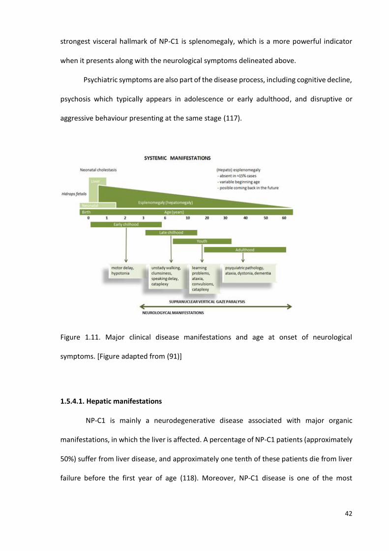
42
strongest visceral hallmark of NP-C1 is splenomegaly, which is a more powerful indicator
when it presents along with the neurological symptoms delineated above.
Psychiatric symptoms are also part of the disease process, including cognitive decline,
psychosis which typically appears in adolescence or early adulthood, and disruptive or
aggressive behaviour presenting at the same stage (117).
Figure 1.11. Major clinical disease manifestations and age at onset of neurological
symptoms. [Figure adapted from (91)]
1.5.4.1. Hepatic manifestations
NP-C1 is mainly a neurodegenerative disease associated with major organic
manifestations, in which the liver is affected. A percentage of NP-C1 patients (approximately
50%) suffer from liver disease, and approximately one tenth of these patients die from liver
failure before the first year of age (118). Moreover, NP-C1 disease is one of the most

43
common disorders responsible for neonatal cholestasis, a disorder in which bilirubin
excretion is altered, and consequently, bile salt levels are decreased in the gastrointestinal
tract, causing a decreased or even null absorption of fats and hydrophobic vitamins (i.e.,
vitamins A, D, E and K). In a 20-year investigation conducted at King’s College Hospital
(London, UK), NP-C disease was found to be the second major cause of neonatal cholestasis,
only one place below alpha-1-antitrypsin deficiency (119). Another 2-year study, performed
in the USA revealed that NP-C was the first cause amongst all metabolic/genetic disorders of
neonatal cholestasis (120).
The liver controls lipoprotein, glucose and cholesterol homeostasis within the body;
it has a major synthetic function producing most of the clotting factors, bile, albumin and
some vitamins. Additionally, the liver has an excretory function (i.e. bilirubin), participates in
the immune response through Kuppfer cells filtering antigens and damaged cells out of the
organ, and has a relevant function in the storage of glycogen and certain vitamins. All these
functions that are performed by this organ, along with the fact that liver disease is one of
the major pathological symptoms of NP-C1, renders investigations involving this organ as a
valuable approach to the disease process.
The majority of investigations on NP-C1 liver have been previously focused on the
lipid profiles of the hepatic cells (121, 122) or alternatively explore hepatocyte gene
expression (123). However, to date low-molecular-mass polar compounds present within
hepatic tissue have not been investigated. Indeed, such metabolites are involved in
metabolic pathways that may be altered in NP-C1 disease.
Studies previously performed using an NP-C mouse model (124) indicate that this
animal model develops a pathological hepatic phenotype similar to that observed in NP-C1
infants (121, 125), showing cholesterol storage, increased levels of liver damage biomarkers
44
such as alkaline phosphatase, aspartate and alanine aminotransferase, hepatomegaly and
the presence of apoptotic cells (122).
1.5.5. Diagnosis
When a patient is suspected to be suffering from NP-C disease, then a genetic test is
carried out to check for mutations in either the NPC1 or NPC2 genes. If at least 1 pathogenic
mutation is detected, then this patient is diagnosed with NP-C (126). Contrarily, if these
pathogenic mutations are not detected, then the filipin test is performed. This diagnostic
test involves the staining of cultured skin fibroblasts from a biopsy obtained from patients,
in order to demonstrate free cholesterol accumulation within lysosomes (127), since this dye
specifically binds unesterified but not esterified cholesterol.
The LDL-induced cholesterol esterification rate assay also represents a useful
complementary evaluation (92). More recently, a preliminary diagnosis of NP-C disease using
the filipin test in a blood smear has been proposed (128), but this demonstrated that there
were no morphological differences between blood samples collected from healthy controls
and NP-C patients; nevertheless, filipin signal intensities were much higher in NP-C patients
than those of healthy controls (128). However, the filipin test gives inconclusive results in
15% of cases (129). If after these tests the NP-C diagnosis is not absolutely clear, further DNA,
mRNA and protein analyses is required.
Recently, diagnostic markers for NP-C such as plasma oxysterols (130) have been
proposed and also the measurement of intracellular acidic compartment volume (mean
equivalent of fluorescence - MEFL/LysoTracker) (131). However, both are complementary to
the above diagnostic methods, and they are required to be more focused on the
development of the disease, its assessment, and its response to treatment. More recently, a
new blood biomarker has been proposed, specifically lysosphingomyelin-509 (a derivative of

45
lyso-sphingomyelin), which is detectable at higher levels in blood collected from NP-C1
patients by LC-MS/MS (132).
1.5.6. Treatment
NP-C presents a complex and wide spectrum of symptoms derived from the
pathophysiology associated with this disease, and different pharmaceutical approaches have
been explored in order to ameliorate the disease process.
NP-C disease also involves behavioural disturbances, catatonia, psychosis and
depression (133); indeed, general psychotic symptoms appear in early adulthood in
approximately 35% of NP-C patients (113). Moreover, in view of the high incidence of
epilepsy in these patients [seizures are common manifestations of the disease in young
patients (134)], anti-epileptic drugs are also employed, including sodium valproate (VPA),
iamotrigin and levetiracetam (135). VPA is also an inhibitor of histone deacetylases (HDACi),
a process that will be further described as a target. However, VPA is one of the weakest and
simplest HDACi, and indeed its performance was not recognized until long after preliminary
studies were performed on its therapeutic properties (136).
Differing medication strategies have been proposed for the treatment of NP-C
disease according to the different classes of its clinical development. Disease-induced
apoptosis has been proposed as one of the targets, so that an inhibitor of protein tyrosine
kinase, imatinib (Gleevec, STI571), was tested against the c-Abl/p73 system, proteins
involved in cerebellar neurodegeneration in NP-C (137). By inhibiting these proteins, Alvarez
et al. reported an increase in Purkinje cell survival, and also a reduction of the apoptotic
process in the cerebellum of NP-C mice; accordingly, neurological symptoms of this mice

46
model were improved, together with a reduction of weight loss coupled with a longer mean
lifespan (137).
A different approach is the therapeutic use of cyclodextrins, which are cyclic
polysaccharides with a truncated cone shape that has the ability to carry hydrophobic
molecules inside its crevice whilst having a hydrophilic outer surface that renders this
polymer soluble in polar solvents and fluids. Cyclodextrin has been proven to ameliorate the
neurological symptoms in NP-C1 disease in the NP-C1 mouse model (BALBc/NPCnih) (138) in
view of its ability to remove cholesterol from neurons; although this process remains
unclear. Furthermore, a cyclodextrin derivative, 2-hydroxypropyl-cyclodextrin has also been
proven to reduce the activation and influx of macrophages in both liver and brain, together
with a corresponding improvement in Purkinge cell survival and consequently a longer
lifespan (139).
Another group of compounds tested for the treatment of NP-C disease are histone
deacetylases. These agents increment the expression of some chaperones that allow mutant
NPC1 proteins to be delivered from the ER to LE/L system. If these NP-C1 mutant proteins
exhibit sufficient activity to export cholesterol from the lysosome, then its accumulation may
be ameliorated as well as the clinical manifestations derived therefrom (140).
In view of the inflammatory processes that take place in the brain of NP-C1 patients
some treatment strategies targeted on the amelioration of this symptom have also been
investigated. The activation of microglial cells and macrophages in the NP-C1 mouse brain
also gives rise to oxidative stress, which has been targeted in combination therapies such as
ibuprofen/aspirin plus vitamin C (141); indeed, in the work performed by Smith et al., they
show how the use of an NSAID such as ibuprofen can improve the lifespan of animals in a
mouse model of NP-C1, based on survival curves (141). Another combined therapy using
47
ibuprofen as an anti-inflammatory agent is its employment with both curcumin and MGS, in
order to target GSL storage (MGS), inflammation (ibuprofen) and calcium homeostasis
(curcumin) (142). In this work, the authors showed how a combination therapy comprising
curcumin and MGS was more efficient than the three drugs together, and then suggested
how anti-inflammatory treatment can ‘act as a double-edged sword’, ameliorating the
symptoms in the first instance and then becoming gradually detrimental, as previously
reported for Sandhoff disease (143), another LSD.
1.5.6.1. Miglustat
One sub-group of iminosugars is the N-iminosugars, in which the anomeric carbon
and the intracyclic oxygen have been replaced by an -NH and a methylene group
respectively. One of the members of this group is miglustat (MGS).
MGS (OGT 918, N-butyl-deoxynojirimycin) is a small molecule (MW = 218) derivative
of a family of polyhydroxylated alkaloids extracted from some plants and micro-organisms,
specifically, a deoxynojirimicyn derivative.
This agent inhibits glucosylceramide synthase and the synthesis of all
glucosylceramide-based GSLs, including lactosylceramide and gangliosides (Figure 1.12),
since this is the first step in glycosphingolipid synthesis (144). The type of inhibition of this
drug was determined by using ceramide as an acceptor, and revealed that
glucosyltransferase activity was competitive for ceramide and non-competitive for UDP-
glucose, confirming that this inhibition was performed by ceramide mimicry (145).
MGS can effectively pass the blood-brain-barrier (BBB), and has the potential to be
effective in treating LSD with neurologic manifestations; indeed, the observational cohort
study carried out by Pineda et al. (115) indicates that MGS stabilizes neurological disease in

48
the majority of patients with NP-C. MGS also provides protection against oxidative stress
(146), which appears to be part of the pathological cascade of symptoms of the disease (146,
147). Moreover, beneficial effects on axonal degeneration were also shown in patients
receiving MGS treatment (148).
Figure 1.12. Key steps in the biosynthesis of GSLs: ceramide glucosyltransferase gives rise to
ceramide glycosylation generating glucosylceramide, a step inhibited by MGS. This
glycosphingolipid is subsequently converted to lactosylceramide which is the precursor of all
the glycosphingolipid series shown.
49
Prior to the approval of MGS as a therapeutic agent for NP-C1 disease, it had been
used to treat other GSL diseases such as Tay-Sachs and Sandhoff diseases (149). Indeed, it
was approved by the European Medicines Agency (EMA) in 2002, and by the USA Food and
Drug Administration (FDA) in 2003 for the treatment of type I Gaucher disease (150, 151).
However, for the treatment of NP-C disease it was only approved in 2009 by the EMA; in
fact, despite its use being approved in most countries, this has not been accomplished in the
USA. It was first proposed for the treatment of this condition based on evidence of slower
disease progression and prolonged survival in animal models (108). Subsequently, clinical
studies demonstrated the stabilization of neurologic disease in both children and adults
treated with MGS (152).
The recommended daily dose is 200 mg 3 x daily in adults, and is adjusted according
to body surface area in patients under 12 years of age (EMA). It was shown to be rapidly
absorbed, and maximal plasma concentrations are attained on average 2.0 - 2.5 hr. after
dosing, on average. Renal clearance is about 150 mL/min (no biotransformations have been
reported), suggesting that the renal elimination is mainly through filtration and also that the
risk for interactions with drugs which are eliminated by active secretion is low (EMA).
MGS was firstly discovered to improve neurological dysfunctions together with an
increase in lifespan in murine and feline NP-C models after its daily administration (153).
Saccadic eye movement velocity, a parameter for disease progression exploration, is
decreased in both the vertical and horizontal direction in NP-C1 patients (154-156);
nonetheless, when these patients receive MGS treatment, this defect is improved (157).
Moreover, about 72% of patients treated with this drug over 12 months presented stabilized
disease status (based on ambulation), swallowing and cognition (158).
50
CHAPTER 2
1H NMR LINKED METABOLOMICS ANALYSIS OF
URINE COLLECTED FROM NP-C1 PATIENTS,
MIGLUSTAT-TREATED PATIENTS AND
HETEROZYGOUS CARRIERS
2.1. URINE SAMPLES PREPARATION FOR NMR ANALYSIS
107 urine samples collected from untreated NP-C1 patients, heterozygote carriers as
controls and miglustat (MGS)-treated patients were stored at -80oC prior to 1H NMR analysis.
Urine samples were provided by Prof. Platt and colleagues at the Department of
Pharmacology, University of Oxford (Oxford, UK); these samples were collected with
informed consent and approved by the appropriate Research Ethics Committee
(06/MRE02/85). Samples were thawed at room temperature, and 0.60 mL of each sample
was centrifuged (5 min., 10,000 x g) in order to remove cells and debris; 0.55 mL of the
supernatant was collected from each sample and subsequently spiked with 0.05 mL of D2O,
thoroughly mixed, and 0.60 mL aliquots of the supernatants were then transferred to 5-mm
diameter NMR tubes (Norell, UK).
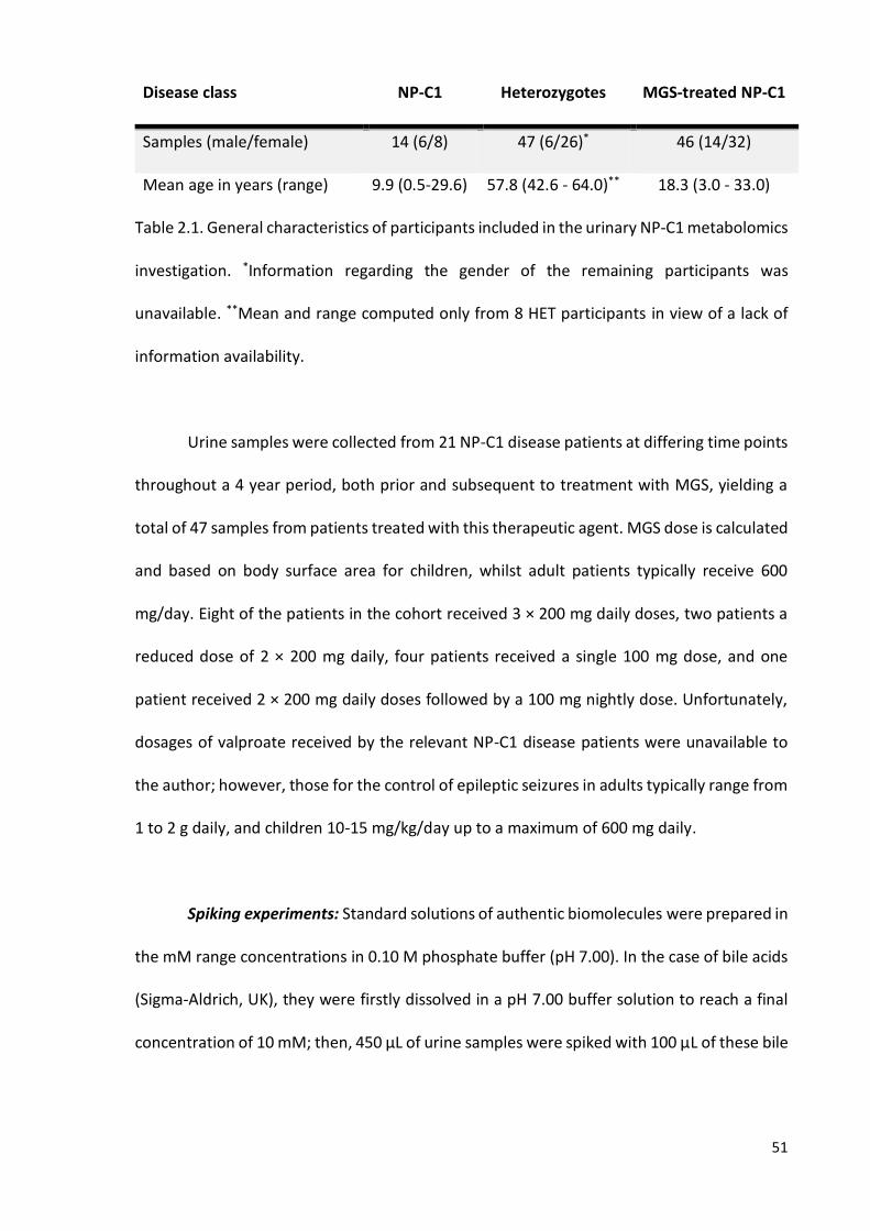
51
Disease class NP-C1 Heterozygotes MGS-treated NP-C1
Samples (male/female) 14 (6/8) 47 (6/26)* 46 (14/32)
Mean age in years (range) 9.9 (0.5-29.6) 57.8 (42.6 - 64.0)** 18.3 (3.0 - 33.0)
Table 2.1. General characteristics of participants included in the urinary NP-C1 metabolomics
investigation. *Information regarding the gender of the remaining participants was
unavailable. **Mean and range computed only from 8 HET participants in view of a lack of
information availability.
Urine samples were collected from 21 NP-C1 disease patients at differing time points
throughout a 4 year period, both prior and subsequent to treatment with MGS, yielding a
total of 47 samples from patients treated with this therapeutic agent. MGS dose is calculated
and based on body surface area for children, whilst adult patients typically receive 600
mg/day. Eight of the patients in the cohort received 3 × 200 mg daily doses, two patients a
reduced dose of 2 × 200 mg daily, four patients received a single 100 mg dose, and one
patient received 2 × 200 mg daily doses followed by a 100 mg nightly dose. Unfortunately,
dosages of valproate received by the relevant NP-C1 disease patients were unavailable to
the author; however, those for the control of epileptic seizures in adults typically range from
1 to 2 g daily, and children 10-15 mg/kg/day up to a maximum of 600 mg daily.
Spiking experiments: Standard solutions of authentic biomolecules were prepared in
the mM range concentrations in 0.10 M phosphate buffer (pH 7.00). In the case of bile acids
(Sigma-Aldrich, UK), they were firstly dissolved in a pH 7.00 buffer solution to reach a final
concentration of 10 mM; then, 450 μL of urine samples were spiked with 100 μL of these bile
52
acids, and 50 μL of D2O containing 0.05% wt. d-TSP) as a lock reference. Subsequently, the
mixture was thoroughly mixed and transferred to a 5-mm diameter NMR tube (Norell, UK).
2.2. NMR ANALYSIS OF NP-C1 URINE SAMPLES
1D 1H NMR: Single-pulse 1H NMR spectra experiments were acquired at 298 K on a
Bruker AX 600 MHz spectrometer (Queen Mary University of London facility, London, UK).
Each spectrum was acquired for 128 scans, 5.6 μs pulses, 32 K (subsequently filled to 65 K)
data points and a spectral width of 12.00 ppm. The intense residual H2O/HDO signal (δ = 4.80
ppm) was supressed using Presaturation (Bruker zgpr pulse sequence). Spectra were
acquired in an automated manner using a sample changer for continuous sample delivery.
1H-1H COSY: These experiment were conducted at 300 K on a Bruker AV 400 MHz
spectrometer (Leicester School of Pharmacy, De Montfort University). The pulse sequence
employed was cosygpprqf (Bruker) with presaturation during relaxation delay using gradient
pulses for selection. The spectral width in the F1 and F2 axes were 4000 Hz, and 2048 data
points were collected in F2. For the urine samples, 256 increments and 32 scans per
increment were used. The relaxation delay was 4.5 s for a total acquisition time of ∼ 7 hr.
Prior to Fourier transformation, a sine function was applied in both time domains.
1H-1H TOCSY: This experiment was carried out at 300 K on a Bruker AV 400 MHz
spectrometer (Leicester School of Pharmacy, De Montfort University). Spectra of urine were
acquired using dipsi2esgpph pulse sequence (Bruker) in which 72 transients per increment
and 256 increments were collected into 2k data points over a spectral width of 12 ppm in
both dimensions applying the MLEV17 spin-lock scheme with a spin-lock power of 6 kHz. A
53
recycle delay of 1.43 s was used, and water suppression was achieved using excitation
sculpting with gradients, and DIPSI2 sequence was employed for mixing. The total acquisition
time per sample was ∼ 18 hr.
1D-TOCSY: 1D TOCSY spectra were acquired using the SELMLGP pulse sequence (1D
homonuclear Hartman-Hahn transfer using MLEV17 sequence for mixing using selective
refocusing with a shaped pulse). This experiment was carried out at 300 K on a Bruker AV
400 MHz spectrometer (Leicester School of Pharmacy, De Montfort University). The mixing
time was set to 0.2 s, 256 FIDs were acquired. The duration of the selective 180° shaped
pulse was optimized to 80 ms and the power level Gauss shape to 63 dB. The 1D-TOCSY pulse
sequence selectively excites only the peak of interest at the specified chemical shift value in
the spectrum, which corresponds to a particular proton/group of protons in a molecule, for
a period of time (the mixing time), in order to transfer this magnetization via J-couplings to
allprotons throughoutthe spinsystem whichitis part of.
2.2.1. 1H NMR Urinary profiles of NP-C1 patients
The identities of metabolites present in the urinary 1H NMR spectra acquired were
assigned according to chemical shift values, coupling patterns and coupling constants and
also from a range of literature sources (45, 159, 160), and then cross-checked with the
Human Metabolome Database (HMDB) (161). A combination of both 1D and 2D COSY and
TOCSY techniques were employed to confirm these assignments, as was the ‛spiking’ of these
biofluids with appropriate small (μL) volumes of solutions of authentic biomolecules
prepared at mM concentrations.

54
(a)
A)
(b)
(c)
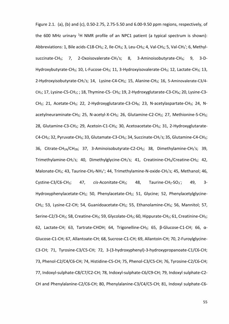
55
Figure 2.1. (a), (b) and (c), 0.50-2.75, 2.75-5.50 and 6.00-9.50 ppm regions, respectively, of
the 600 MHz urinary 1H NMR profile of an NPC1 patient (a typical spectrum is shown):
Abbreviations: 1, Bile acids-C18-CH3; 2, Ile-CH3; 3, Leu-CH3; 4, Val-CH3; 5, Val-CH3'; 6, Methyl-
succinate-CH3; 7, 2-Oxoisovalerate-CH3's; 8, 3-Aminoisobutyrate-CH3; 9, 3-D-
Hydroxybutyrate-CH3; 10, L-Fucose-CH3; 11, 3-Hydroxyisovalerate-CH3; 12, Lactate-CH3; 13,
2-Hydroxyisobutyrate-CH3's; 14, Lysine-C4-CH2; 15, Alanine-CH3; 16, 5-Aminovalerate-C3/4-
CH2; 17, Lysine-C5-CH2; ; 18, Thymine-C5- CH3; 19, 2-Hydroxyglutarate-C3-CHA; 20, Lysine-C3-
CH2; 21, Acetate-CH3; 22, 2-Hydroxyglutarate-C3-CHB; 23, N-acetylaspartate-CH3; 24, N-
acetylneuraminate-CH3; 25, N-acetyl-X-CH3; 26, Glutamine-C2-CH2; 27, Methionine-S-CH3;
28, Glutamine-C3-CH2; 29, Acetoin-C1-CH3; 30, Acetoacetate-CH3; 31, 2-Hydroxyglutarate-
C4-CH2; 32, Pyruvate-CH3; 33, Glutamate-C3-CH2; 34, Succinate-CH2's; 35, Glutamine-C4-CH2;
36, Citrate-CH2A/CH2B; 37, 3-Aminoisobutyrate-C2-CH2; 38, Dimethylamine-CH3's; 39,
Trimethylamine-CH3's; 40, Dimethylglycine-CH3's; 41, Creatinine-CH3/Creatine-CH3; 42,
Malonate-CH2; 43, Taurine-CH2-NH3+; 44, Trimethylamine-N-oxide-CH3's; 45, Methanol; 46,
Cystine-C3/C6-CH2; 47, cis-Aconitate-CH2; 48, Taurine-CH2-SO3-; 49, 3-
Hydroxyphenylacetate-CH2; 50, Phenylacetate-CH2; 51, Glycine; 52, Phenylacetylglycine-
CH2; 53, Lysine-C2-CH; 54, Guanidoacetate-CH2; 55, Ethanolamine-CH3; 56, Mannitol; 57,
Serine-C2/3-CH2; 58, Creatine-CH2; 59, Glycolate-CH2; 60, Hippurate-CH2; 61, Creatinine-CH2;
62, Lactate-CH; 63, Tartrate-CHOH; 64, Trigonelline-CH3; 65, β-Glucose-C1-CH; 66, α-
Glucose-C1-CH; 67, Allantoate-CH; 68, Sucrose-C1-CH; 69, Allantoin-CH; 70, 2-Furoylglycine-
C3-CH; 71, Tyrosine-C3/C5-CH; 72, 3-(3-hydroxyphenyl)-3-hydroxypropanoate-C1/C6-CH;
73, Phenol-C2/C4/C6-CH; 74, Histidine-C5-CH; 75, Phenol-C3/C5-CH; 76, Tyrosine-C2/C6-CH;
77, Indoxyl-sulphate-C8/C7/C2-CH; 78, Indoxyl-sulphate-C6/C9-CH; 79, Indoxyl sulphate-C2-
CH and Phenylalanine-C2/C6-CH; 80, Phenylalanine-C3/C4/C5-CH; 81, Indoxyl sulphate-C6-

56
CH and Benzoate-C3/C5-CH; 82, Hippurate-C3/C5-CH: 83, Hippurate-C4-CH; 84, 1-
Methylhistidine-C4-CH; 85, Hippurate-C2/C6-CH; 86, Histidine-C2-CH; 87, 3-Methylhistidine-
C2-CH; 88, Quinolinate-C5-CH; 89, 3-Methylxanthine-C7-CH; 90, Trigonelline-C5-CH; 91,
Hypoxanthine-C2/C7-CH; 92, 1-Methylnicotinamide-C5-CH; 93, Quinolinate-C6-CH; 94,
Formate-H; 95, Trigonelline-C4/C6-CH; 96, Trigonelline-C2-CH; 97, N-methylnicotinamide-
C2-CH; 98, N-Ribosylnicotinamide-C2-CH.
Typical 600 MHz single-pulse 1H NMR spectra of urine samples collected from NP-C1
disease patients and their heterozygous carrier controls contained a multitude of prominent,
sharp signals assignable to a wide range of low molecular-mass metabolites (Figure 2.1).
Indeed, resonances ascribable to a very wide range of amino acids [e.g. glycine (Gly), alanine
(Ala), leucine (Leu), isoleucine (Ile), valine (Val), tyrosine (Tyr) and taurine, etc.], short-chain
organic acid anions (e.g., acetate, citrate, formate, fumarate, lactate, pyruvate, succinate,
etc.), amines such as methyl-, dimethyl- and trimethylamines, and bile acids, together with
many further classes of biomolecules, were readily observable. Indeed, > 100 different
metabolites were unambiguously assigned on the basis of the 107 spectra acquired. Some
resonances present in the spectra required further work in order to confirm assignments in
addition to the simple acquisition of a 1D spectrum, and therefore correlation spectroscopic
techniques were applied, such as TOCSY (in both 1D and 2D versions) and COSY. The coupling
patterns of the metabolites can be explored by performing these correlation spectroscopy
experiments, as can be observed in Figure 2.2, in which 3-aminoisobutyrate (3-AIB) was
identified in urine samples using a 1D-TOCSY experiment.
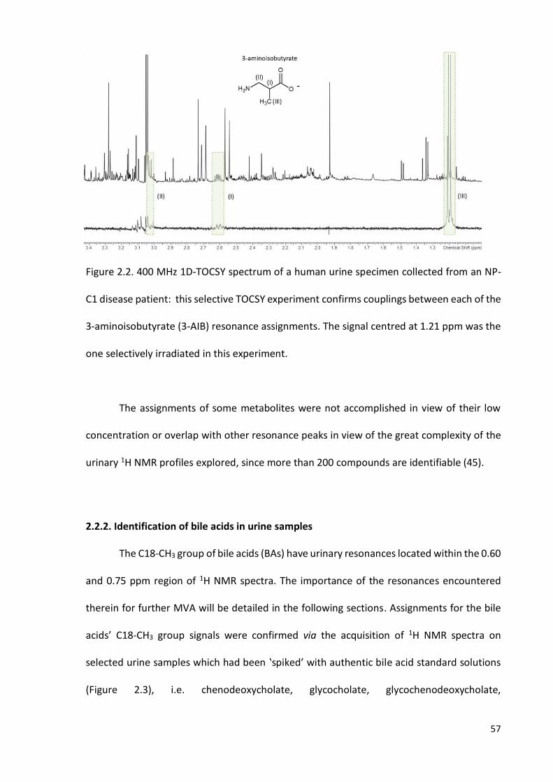
57
Figure 2.2. 400 MHz 1D-TOCSY spectrum of a human urine specimen collected from an NP-
C1 disease patient: this selective TOCSY experiment confirms couplings between each of the
3-aminoisobutyrate (3-AIB) resonance assignments. The signal centred at 1.21 ppm was the
one selectively irradiated in this experiment.
The assignments of some metabolites were not accomplished in view of their low
concentration or overlap with other resonance peaks in view of the great complexity of the
urinary 1H NMR profiles explored, since more than 200 compounds are identifiable (45).
2.2.2. Identification of bile acids in urine samples
The C18-CH3 group of bile acids (BAs) have urinary resonances located within the 0.60
and 0.75 ppm region of 1H NMR spectra. The importance of the resonances encountered
therein for further MVA will be detailed in the following sections. Assignments for the bile
acids’ C18-CH3 group signals were confirmed via the acquisition of 1H NMR spectra on
selected urine samples which had been ‛spiked’ with authentic bile acid standard solutions
(Figure 2.3), i.e. chenodeoxycholate, glycocholate, glycochenodeoxycholate,

58
taurochenodeoxycholate, taurodeoxycholate and tauroursodeoxycholate. Lithocholate
solubility in water is only ca. 0.05 µM (162), and therefore, it is unobservable by either 400
MHz or 600 MHz NMR spectrometers; accordingly, its C18-CH3 resonance was not observed
in Figure 2.3(a).
Figure 2.3. (a) 0.4 - 1.1 ppm region from a 400 MHz 1H NMR spectra of a urine sample ‛spiked’
with different bile acids (BAs): the C18-CH3 group signal can be clearly observed as a singlet
between 0.65 and 0.75 ppm. The green shadowed rectangle highlights the 0.66 - 0.69 ppm
bucket. (b) BAs general chemical structure together with a table listing those BAs arising from
the different possible substitutions in those groups highlighted. Glycine or taurine adducts
resulting from further conjugations are located at R1.

59
BAs that do not present an -OH group in either C7 or C12 [Figure 2.4 (b)] positions
are responsible for this signal, since BAs that do have a downfield-shifted C18-CH3 resonance
contain a hydroxyl group. Indeed, the more pronounced effect is ascribed to C12, as
expected in view of its proximity to C18. The conjugation with either taurine or glycine does
not exert any major observable effects on the chemical shift value of this C18-CH3 resonance
[Figure 2.3 (a)]. Additionally, p-values arising from the ANOVA model depicted in Equation
19 for adjacent regions to the 0.66-0.69 ppm bucket were not significant for the comparison
between HET and NPC groups [p (0.61 - 0.66 ppm) = 0.211), p (0.69 - 0.72 ppm) = 0.728].
2.3. DATA PREPROCESSING
61 urine samples were initially included for statistical analysis: 14 untreated NP-C1
patients (NPC) and 47 heterozygous carriers as controls (HET). The binning process gave a
table of 61 rows (samples) x 199 columns (variables), containing the sum-normalised
intensities of each spectrum. Spectral regions containing resonances arising from ethanol (t,
1.22 - 1.24 ppm; q, 3.63 - 3.67 ppm), which were detectable in several of the heterozygous
carrier urine samples and urea (br, 5.59 - 5.99 ppm) were removed from all the urinary 1H
NMR profiles for further MVA.
An exponential line-broadening function of 0.30 Hz was routinely applied to the FIDs
prior to FT for all the spectra that were subsequently phased, baseline corrected and
referenced to the formate (s, 8.46 ppm) resonance since no internal standard was added to
the samples. Moreover, the formate-H resonance is readily visible as a singlet in a clear
region of the urinary NMR profiles, and therefore it is easily identifiable. The intense δ = 4.65
- 5.15 ppm residual H2O/HDO signal region was also removed from all the 1H NMR profiles
acquired prior to the performance of MV data analysis strategies.
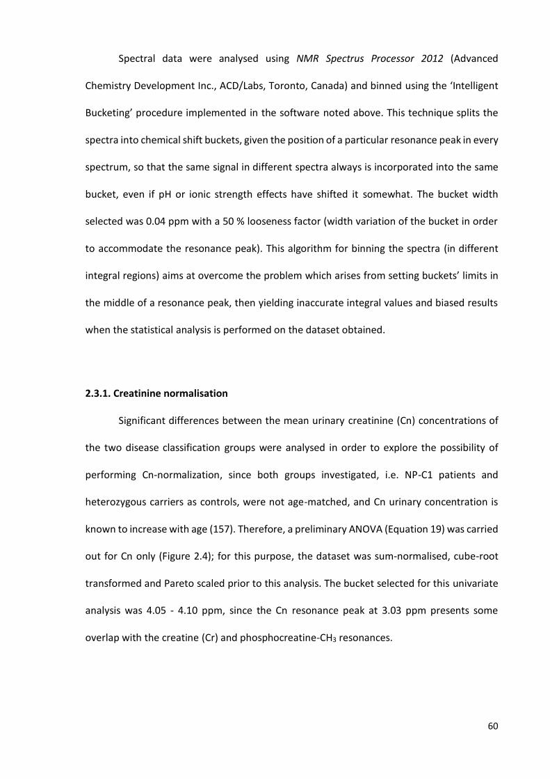
60
Spectral data were analysed using NMR Spectrus Processor 2012 (Advanced
Chemistry Development Inc., ACD/Labs, Toronto, Canada) and binned using the ‘Intelligent
Bucketing’ procedure implemented in the software noted above. This technique splits the
spectra into chemical shift buckets, given the position of a particular resonance peak in every
spectrum, so that the same signal in different spectra always is incorporated into the same
bucket, even if pH or ionic strength effects have shifted it somewhat. The bucket width
selected was 0.04 ppm with a 50 % looseness factor (width variation of the bucket in order
to accommodate the resonance peak). This algorithm for binning the spectra (in different
integral regions) aims at overcome the problem which arises from setting buckets’ limits in
the middle of a resonance peak, then yielding inaccurate integral values and biased results
when the statistical analysis is performed on the dataset obtained.
2.3.1. Creatinine normalisation
Significant differences between the mean urinary creatinine (Cn) concentrations of
the two disease classification groups were analysed in order to explore the possibility of
performing Cn-normalization, since both groups investigated, i.e. NP-C1 patients and
heterozygous carriers as controls, were not age-matched, and Cn urinary concentration is
known to increase with age (157). Therefore, a preliminary ANOVA (Equation 19) was carried
out for Cn only (Figure 2.4); for this purpose, the dataset was sum-normalised, cube-root
transformed and Pareto scaled prior to this analysis. The bucket selected for this univariate
analysis was 4.05 - 4.10 ppm, since the Cn resonance peak at 3.03 ppm presents some
overlap with the creatine (Cr) and phosphocreatine-CH3 resonances.
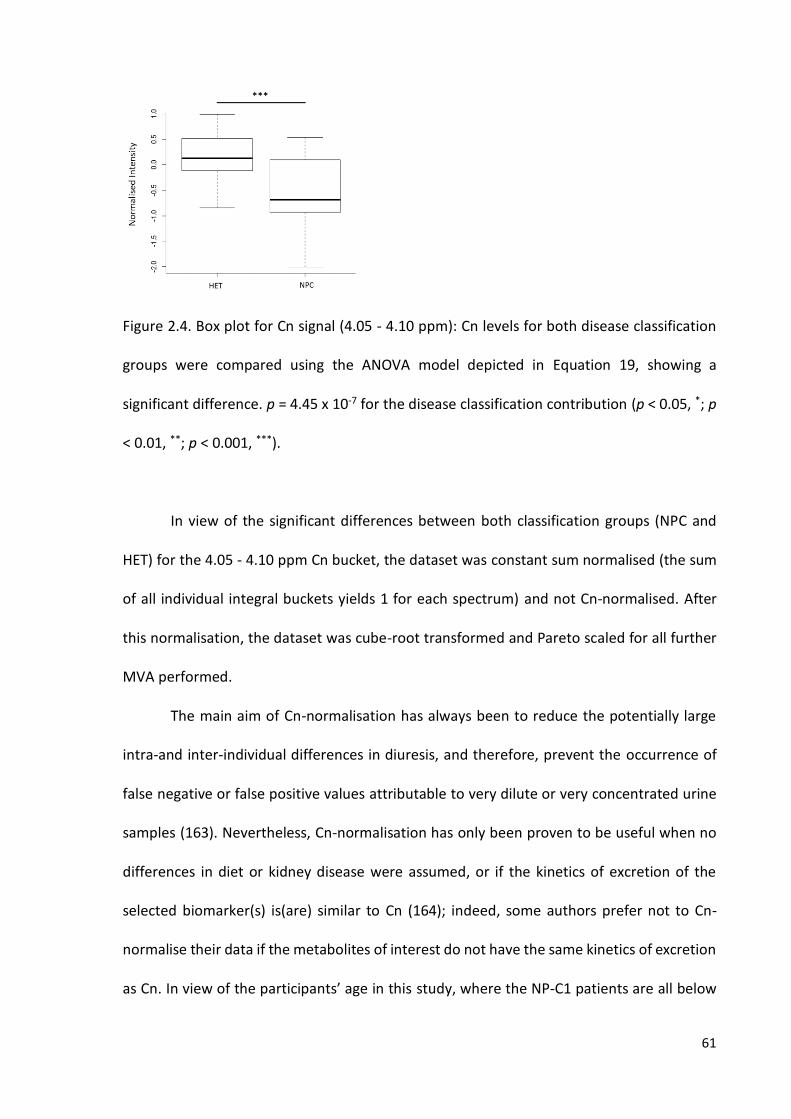
61
Figure 2.4. Box plot for Cn signal (4.05 - 4.10 ppm): Cn levels for both disease classification
groups were compared using the ANOVA model depicted in Equation 19, showing a
significant difference. p = 4.45 x 10⁻⁷ for the disease classification contribution (p < 0.05, *; p
< 0.01, **; p < 0.001, ***).
In view of the significant differences between both classification groups (NPC and
HET) for the 4.05 - 4.10 ppm Cn bucket, the dataset was constant sum normalised (the sum
of all individual integral buckets yields 1 for each spectrum) and not Cn-normalised. After
this normalisation, the dataset was cube-root transformed and Pareto scaled for all further
MVA performed.
The main aim of Cn-normalisation has always been to reduce the potentially large
intra-and inter-individual differences in diuresis, and therefore, prevent the occurrence of
false negative or false positive values attributable to very dilute or very concentrated urine
samples (163). Nevertheless, Cn-normalisation has only been proven to be useful when no
differences in diet or kidney disease were assumed, or if the kinetics of excretion of the
selected biomarker(s) is(are) similar to Cn (164); indeed, some authors prefer not to Cn-
normalise their data if the metabolites of interest do not have the same kinetics of excretion
as Cn. In view of the participants’ age in this study, where the NP-C1 patients are all below

62
32 years of age and the HET participants are the parents of those donors, the expected result
for Cn levels matches with the one obtained in the ANOVA performed. The p-values obtained
therefrom indicated significatively higher Cn levels for the HET group, and therefore, Cn-
normalisation was discarded for MVA of the urinary dataset.
Prior to performing both univariate and MVA, samples were visually checked for any
major disturbances. One NP-C1 patient was found to be receiving valproate treatment by
detecting a triplet at 0.84 ppm and its coupling with the remaining valproate-CH2’s resonance
signals, and 6 heterozygous carriers plus another NP-C1 patient taking acetaminophen, since
their characteristic resonance signals were identified at 7.13 and 7.35 ppm for its glucuronide
metabolite, 7.31 and 7.45 ppm for the sulphate one and 2.16 ppm for its acetamido methyl
group (Figure 2.11). All these samples were removed for the purpose of all further analysis.
2.4. UNIVARIATE AND MULTIVARIATE ANALYSIS OF THE 1H NMR URINARY DATASET
2.4.1. Univariate data analysis: ANOVA
ANOVA analysis of the urinary dataset was performed according to the model
depicted in Equation 19 to explore any significant differences between the metabolites for
each disease group, and also to isolate the variance attributable to the disease status,
removing any further effect attributable to kinship. In this ANOVA model, Yijk represents the
(univariate) predictor variable value observed, µ is the overall population mean value in the
absence of any significant, influential sources of variation. Di, Fj and DFij are components of
variation ascribable to between-disease classifications, family, and the disease classification-
family interaction sources, and eij is the unexplained error (residual) contribution.
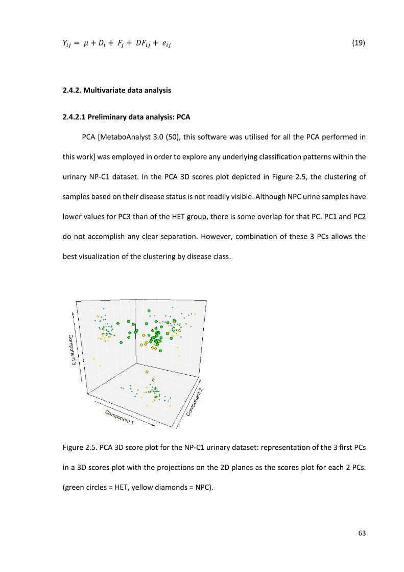
63
𝑌𝑖𝑗 = 𝜇 + 𝐷𝑖 + 𝐹𝑗 + 𝐷𝐹𝑖𝑗 + 𝑒𝑖𝑗 (19)
2.4.2. Multivariate data analysis
2.4.2.1 Preliminary data analysis: PCA
PCA [MetaboAnalyst 3.0 (50), this software was utilised for all the PCA performed in
this work] was employed in order to explore any underlying classification patterns within the
urinary NP-C1 dataset. In the PCA 3D scores plot depicted in Figure 2.5, the clustering of
samples based on their disease status is not readily visible. Although NPC urine samples have
lower values for PC3 than of the HET group, there is some overlap for that PC. PC1 and PC2
do not accomplish any clear separation. However, combination of these 3 PCs allows the
best visualization of the clustering by disease class.
Figure 2.5. PCA 3D score plot for the NP-C1 urinary dataset: representation of the 3 first PCs
in a 3D scores plot with the projections on the 2D planes as the scores plot for each 2 PCs.
(green circles = HET, yellow diamonds = NPC).

64
2.4.2.2. Classification performance
Random Forests (RFs): The RFs technique was employed for classification and
variable selection purposes using the randomForest R package (165) (this software was
utilised for all the RF analysis performed in this work).
RFs parameters were tuned in order to improve its performance, so the number of
trees was set up to 500 and the number of variables selected at each split was 8 based on
the Out-Of-Bag (OOB) error values obtained. RFs was applied over 100 iterations; at each
iteration, the OOB and the confusion matrix was stored in order to obtain classification
performance parameters (Table 2.2). Additionally, variable importance (mean decrease
accuracy criterion, MDA) values for variable selection were extracted and their mean and
standard error of the mean (SEM) values computed. For each set of 100 iterations, a column
of 65 rows (number of samples) was generated containing random numbers from 0 to 1, so
that samples with values > 0.66 were included in the test-set, whilst samples with values ≤
0.66 were included in the training-set. This procedure, also known as Monte Carlo Cross-
Validation (MCCV) was applied to each class (NPC and HET) independently.
Genetic Algorithms (GAs): The GAs strategy was applied using the GALGO R-package
(166) that allows the selection of different parametric and non-parametric classification
techniques such as k-nearest-neighbours, discriminant functions (Maximum Likelihood),
nearest centroid, SVMs, RFs and neural networks. In this work we have used SVMs and
MLHD.
For this GAs methodology, the chromosome size was selected to be 10 (maximum
number of variables in each model/chromosome). These chromosomes evolved generating
500 solutions (chromosomes/models) with the aim of achieving a fitness value of 0.9. To
65
build up the models, the methods employed were Maximum LikeliHooD (MLHD, a
modification of LDA that uses Bayes’ rule as the discriminant function assigning a sample to
the class with highest conditional probability) and SVMs, using a radial Kernel. The
performance of the models generated using the techniques delineated above was computed
by using a 5-fold cross validation procedure and the outcomes are listed in Table 2.2.
Correlated Component Regression-Linear Discriminant Analysis (CCR-LDA): CCR-LDA
was set to a maximum of 1, 2 and 3 components and to a maximum of 5, 10, 15 and 20
variables for developing the classification models. Each of the combinations was repeated 5
times, resulting in 60 different models. The validation procedure was a 5-fold cross-
validation over 10 rounds. Results from this CCR-LDA analysis are shown in Table 2.2.
Table 2.2. Classification performance of the techniques employed for the analysis of the NP-
C1 urinary dataset: the OOB error value is also indicated for the RFs approach. Standard error
of the mean values for each of the parameters computed are provided in brackets.
All the MVA techniques were able to succesfully classify urine samples regarding their
disease status (NPC vs. HET); indeed, they all gave very good results for specificity and
accuracy. However, values obtained for sensitivity were not very efficient, the CCR-LDA
technique having the lowest sensitivity and the highest variablity, not only for sensitivity, but
MVA Technique OOB (SEM) Accuracy (SEM) Sensitivity (SEM) Specificity (SEM)
RFs 0.224 (0.00012) 0.835 (0.001) 0.695 (0.001) 0.831 (0.003)
GA-MLHD/SVM - 0.827 (0.002) 0.752 (0.002) 0.903 (0.001)
CCR-LDA - 0.810 (0.013) 0.583 (0.032) 0.926 (0.012)
66
for the remainder of the classification performance parameters computed, as observed for
the SEM values displayed in Table 2.2. However, these SEM values cannot be considered
high, since the maximum value accounts for only 5.49% of the averaged sensitivity
parameter. Nevertheless, the CCR-LDA model gave the highest specificity value (0.926). The
RFs and CCR-LDA strategies gave the highest accuracy and specificity values respectively
when applied to the NP-C1 urinary dataset.
The limitations introduced for GAs and CCR-LDA classifications technique with regard
of the number of variables that could be included to the model building process were aimed
at reducing the neglective effect of overfitting, i.e. the employment of a number of variables
highly exceeding the number of samples, which results in very accurate models which usually
fail when new samples are tested. Additionally, cross-validation procedures were
implemented in the model development process in order to also overcome this issue.
2.4.2.3. Variable Selection
Random Forests (RFs): Throughout the 100 iterations applied in the RFs analysis
outlined above, MDA value for variable importance was computed, and consequently, the
mean value of those 100 MDAs obtained for each variable; so that a variable ranking was
obtained on completion of the process (Table 2.3).
Genetic Algorithms (GAs): The GALGO package saves the frequency at which each
variable is selected to generate a successful classification (i.e., reach a fitness of 0.9). The
variables can then be ranked and averaged for both techniques (SVMs and MHLD) based on
these frequencies (Table 2.3).
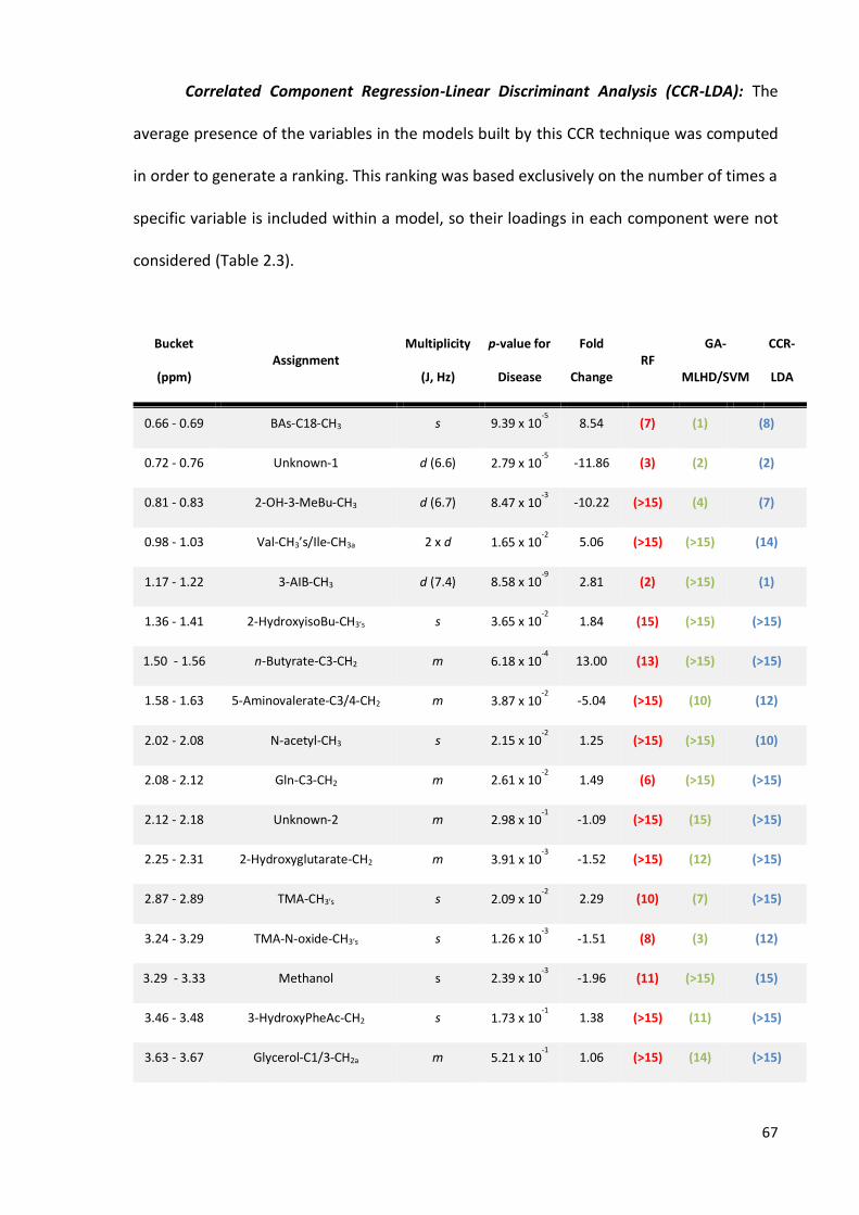
67
Correlated Component Regression-Linear Discriminant Analysis (CCR-LDA): The
average presence of the variables in the models built by this CCR technique was computed
in order to generate a ranking. This ranking was based exclusively on the number of times a
specific variable is included within a model, so their loadings in each component were not
considered (Table 2.3).
Bucket
(ppm) Assignment
Multiplicity
(J, Hz)
p-value for
Disease
Fold
Change RF
GA-
MLHD/SVM
CCR-
LDA
0.66 - 0.69 BAs-C18-CH3 s 9.39 x 10⁻⁵
8.54 (7) (1) (8)
0.72 - 0.76 Unknown-1 d (6.6) 2.79 x 10⁻⁵
-11.86 (3) (2) (2)
0.81 - 0.83 2-OH-3-MeBu-CH3 d (6.7) 8.47 x 10⁻³
-10.22 (>15) (4) (7)
0.98 - 1.03 Val-CH3’s/Ile-CH3a 2 x d 1.65 x 10⁻²
5.06 (>15) (>15) (14)
1.17 - 1.22 3-AIB-CH3 d (7.4) 8.58 x 10⁻⁹
2.81 (2) (>15) (1)
1.36 - 1.41 2-HydroxyisoBu-CH3’s s 3.65 x 10⁻²
1.84 (15) (>15) (>15)
1.50 - 1.56 n-Butyrate-C3-CH2 m 6.18 x 10⁻⁴
13.00 (13) (>15) (>15)
1.58 - 1.63 5-Aminovalerate-C3/4-CH2 m 3.87 x 10⁻²
-5.04 (>15) (10) (12)
2.02 - 2.08 N-acetyl-CH3 s 2.15 x 10⁻²
1.25 (>15) (>15) (10)
2.08 - 2.12 Gln-C3-CH2 m 2.61 x 10⁻²
1.49 (6) (>15) (>15)
2.12 - 2.18 Unknown-2 m 2.98 x 10⁻¹
-1.09 (>15) (15) (>15)
2.25 - 2.31 2-Hydroxyglutarate-CH2 m 3.91 x 10⁻³
-1.52 (>15) (12) (>15)
2.87 - 2.89 TMA-CH3’s s 2.09 x 10⁻²
2.29 (10) (7) (>15)
3.24 - 3.29 TMA-N-oxide-CH3’s s 1.26 x 10⁻³
-1.51 (8) (3) (12)
3.29 - 3.33 Methanol s 2.39 x 10⁻³
-1.96 (11) (>15) (15)
3.46 - 3.48 3-HydroxyPheAc-CH2 s 1.73 x 10⁻¹
1.38 (>15) (11) (>15)
3.63 - 3.67 Glycerol-C1/3-CH2a m 5.21 x 10⁻¹
1.06 (>15) (14) (>15)
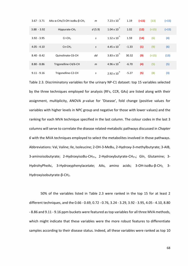
68
3.67 - 3.71 AAs-α-CHs/3-OH-isoBu-β-CH2 m 7.23 x 10⁻²
1.19 (>15) (13) (>15)
3.88 - 3.92 Hippurate-CH2 d (5.9) 1.04 x 10⁻¹
1.02 (12) (>15) (>15)
3.92 - 3.95 Cr-CH2 s 1.52 x 10⁻⁵
1.59 (14) (6) (4)
4.05 - 4.10 Cn-CH3 s 4.45 x 10⁻⁷
-1.33 (1) (9) (6)
8.40 - 8.42 Quinolinate-C6-CH dd 3.83 x 10⁻⁵
30.32 (9) (>15) (13)
8.80 - 8.86 Trigonelline-C4/6-CH m 4.96 x 10⁻⁴
-6.70 (4) (5) (5)
9.11 - 9.16 Trigonelline-C2-CH s 2.92 x 10⁻⁴
-5.27 (5) (8) (3)
Table 2.3. Discriminatory variables for the urinary NP-C1 dataset: top 15 variables selected
by the three techniques employed for analysis (RFs, CCR, GAs) are listed along with their
assignment, multiplicity, ANOVA p-value for ‛Disease’, fold change (positive values for
variables with higher levels in NPC group and negative for those with lower values) and the
ranking for each MVA technique specified in the last column. The colour codes in the last 3
columns will serve to correlate the disease related-metabolic pathways discussed in Chapter
6 with the MVA techniques employed to select the metabolites involved in those pathways.
Abbreviations: Val, Valine; Ile, Isoleucine; 2-OH-3-MeBu, 2-Hydroxy-3-methylbutyrate; 3-AIB,
3-aminoisobutyrate; 2-HydroxyisoBu-CH3’s, 2-Hydroxybutyrate-CH3’s; Gln, Glutamine; 3-
HydrohyPheAc, 3-Hydroxyphenylacetate; AAs, amino acids; 3-OH-isoBu-β-CH2, 3-
Hydroxyisobutyrate-β-CH2.
50% of the variables listed in Table 2.3 were ranked in the top 15 for at least 2
different techniques, and the 0.66 - 0.69, 0.72 - 0.76, 3.24 - 3.29, 3.92 - 3.95, 4.05 - 4.10, 8.80
- 8.86 and 9.11 - 9.16 ppm buckets were featured as top variables for all three MVA methods,
which might indicate that these variables were the more robust features to differentiate
samples according to their disease status. Indeed, all these variables were ranked as top 10

69
features for all the techniques, and only the 1.17 - 1.22 ppm bucket, despite not being
selected by the GAs approach, it should be included as a top important variable since it was
ranked 2nd and 1st by RFs and CCR-LDA respectively.
The major discriminatory variables include branched chain amino acids (BCAAs) such
as Ile and Val, and products of their degradation pathways such as 3-AIB, 2-hydroxy-3-
methylbutyrate and 3-hydroxyisobutyrate; moreover, Gln, 3-hydroxyphenylacetate (a
tyrosine metabolite) and the α-group resonance signal from amino acids were also selected.
This bile acid bucket has been highlighted as one of the most important features as
well, although the exact bile acids species contributing to this signal are somewhat unclear.
n-Butyrate is a gut microbiota metabolite arising from carbohydrate fermentation.
Further metabolites listed in Table 2.3 that can also be attributed to gut microflora are TMA
(choline degradation product) and 5-aminovalerate, the latter a product of lysine catabolism.
Higher levels of TMA-N-oxide (TMAO), trigonelline and Cn were observed in the HET
participants; however, these three metabolites are well known age-correlated metabolites
which may arise from diet (TMAO and trigonelline) and muscle tissue (Cn).
Three metabolites listed in Table 2.3, could arise from exogenous sources as 2-
hydroxyisobutyrate and methanol (although methanol also arises from microflora
metabolism), in addition to hippurate, a metabolite of benzoate mainly encountered in plant
dietary sources and a gut microbial-mammalian co-metabolite generated through the
conjugation of benzoate with glycine (167).
The N-acetyl-group signals arise from the acetamido (-NHCOCH3) groups of some
metabolites as a result of a common chemical modification, frequently encountered in
amino acids and sugars, mainly occurring in brain.

70
2-Hydroxyglutarate is a hydroxy-acid resulting from the reduction of ketoglutarate,
an intermediate in the Krebs cycle.
Quinolinate is a product of kynurenine metabolism and a precursor of niacin
nucleotides, such as NAD, NADP, etc. that can also act as a neurotransmitter.
Glycerol is a structural metabolite being the frame for the addition of fatty acids to
form triacylglycerols (TG), diacylglycerols (DG) and monoacylglycerols (MG).
One of the most important variables selected was the 0.72 - 0.76 ppm bucket, which
remains unassigned, although it has been previously reported in urine (168); indeed, the
coupling constant (J) value of this resonance signal (6.6 Hz) is very similar to that determined
in (168) (6.8 Hz), and these researchers have suggested that it arises from the -CH3 unit of an
isopropyl group, which is linked to a magnetically-distinguishable, second -CH3 group doublet
resonance located at δ = 0.88 ppm. Both these -CH3 units were found to be connected (albeit
in a MV statistical context) to a suggested asymmetrical carbon atom methine (-CH)
fragment (centred at δ = 2.18 ppm), although these investigators did not confirm these
connectivities via the application of neither 1D or 2D 1H-1H NMR COSY/TOCSY techniques.
2.4.2.4. ROC curve analysis
Biomarker selection was investigated through ROC curve analysis. This analysis was
conducted using the ROC curve analysis option included in MetaboAnalyst 3.0 [(169) this
software was utilised for all the ROC curve analysis performed in this work]. Those
metabolites selected as discriminatory features for more than 1 of the techniques in Table
2.3, excluding those likely arising from age differences between both disease-classification
groups, were subjected to ROC curve analysis in order to explore their ability as NP-C1
disease urinary biomarkers. The variables selected were those assigned to bile acids (0.66 -

71
0.69 ppm), unknown metabolite (0.72 - 0.76 ppm), 2-hydroxy-3-methylbutyrate-CH3a (0.81 -
0.83 ppm), 3-AIB-CH3 (1.17 - 1.22 ppm), 5-aminovalerate-C3/4-CH2, (1.58 - 1.63 ppm),
trimethylamine-CH3’s (2.87 - 2.89 ppm), methanol (3.29 - 3.33 ppm), creatine (3.92 - 3.95
ppm) and quinolinate (8.40 - 8.42 ppm). However, the presence of methanol must be taken
cautiously since their higher levels in the HET group could be attributable to the lowest
exposure to methanol vapours (cleaning products) and alcohol consumption in the younger
NP-C1 patients (170).
Figure 2.6. (a) ROC curves and (b) bubbles diagram for variable importance in the NP-C1
urinary dataset: different combinations of variables gave different AUC values ranging from
0.705 for 2 variables, up to 0.918 with 8 variables, as indicated in the table inserted in (a).
Variable ranking arising from ROC analysis is depicted in the vertical axis in (b), blue bubbles
indicate metabolites with lower levels in NPC group, and the orange ones, those with higher
levels. The size of each bubble is correlated with the FC (fold change). Abbreviations: U-1,
72
unknown metabolite; 2-OH-3-MeBu, 2-Hydroxy-3-methylbutyrate; TPR, True Positive Rate;
FPR, False Positive Rate.
The assessment of model performance is evaluated through MCCV, so that two-
thirds of the samples were utilised in order to generate a RFs classifier which were validated
on the one-third of the remaining samples excluded from the model building process; the
sensitivity and specificity of the models developed were computed from the confusion
matrix arising from the multiple MCCV iterations. 100 rounds of CV were performed, and
results were depicted in the form of a ROC curve by plotting the sensitivity against 1-
specificity showing the performance of biomarkers subsets. Through this method, the
models generated combine different features in each case from the maximum number of
variables entered.
As expected, mean AUC values were decreasing along with the number of variables
employed for the model, apart from the model built up with 8 variables that has higher
values than the 9 variables one. AUC values were all above 0.7, a performance which is
consider fair, in terms of classification success. The selection frequencies of those 9 variables
included in the ROC analysis are illustrated in Figure 2.6 along with their fold change (FC).
Bile acids, an unknown doublet within the δ = 0.72-0.76 ppm bucket, 2-hydroxy-3-
methylbutyrate and 3-AIB were the metabolites most frequently selected for construction
of the models.
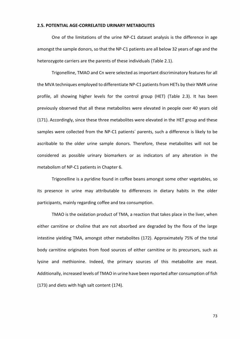
73
2.5. POTENTIAL AGE-CORRELATED URINARY METABOLITES
One of the limitations of the urine NP-C1 dataset analysis is the difference in age
amongst the sample donors, so that the NP-C1 patients are all below 32 years of age and the
heterozygote carriers are the parents of these individuals (Table 2.1).
Trigonelline, TMAO and Cn were selected as important discriminatory features for all
the MVA techniques employed to differentiate NP-C1 patients from HETs by their NMR urine
profile, all showing higher levels for the control group (HET) (Table 2.3). It has been
previously observed that all these metabolites were elevated in people over 40 years old
(171). Accordingly, since these three metabolites were elevated in the HET group and these
samples were collected from the NP-C1 patients´ parents, such a difference is likely to be
ascribable to the older urine sample donors. Therefore, these metabolites will not be
considered as possible urinary biomarkers or as indicators of any alteration in the
metabolism of NP-C1 patients in Chapter 6.
Trigonelline is a pyridine found in coffee beans amongst some other vegetables, so
its presence in urine may attributable to differences in dietary habits in the older
participants, mainly regarding coffee and tea consumption.
TMAO is the oxidation product of TMA, a reaction that takes place in the liver, when
either carnitine or choline that are not absorbed are degraded by the flora of the large
intestine yielding TMA, amongst other metabolites (172). Approximately 75% of the total
body carnitine originates from food sources of either carnitine or its precursors, such as
lysine and methionine. Indeed, the primary sources of this metabolite are meat.
Additionally, increased levels of TMAO in urine have been reported after consumption of fish
(173) and diets with high salt content (174).

74
Cn is a by-product of muscle metabolism arising from Cr-phosphate breakdown,
which is subsequently excreted into urine. Urinary excretion of Cn correlates positively with
body weight, reflecting skeletal muscle mass (175, 176), and therefore, higher
concentrations are expected in adults. Daily urinary excretion of Cn derived from muscles
occurs at a ratio of ca. 1 g per 20 kg of muscle mass (177).
2.6. NMR ANALYSIS OF URINE SAMPLES COLLECTED FROM NP-C1 PATIENTS
UNDERGOING MIGLUSTAT TREATMENT
2.6.1 NMR characterization of miglustat
Prior to the detection of MGS in urine, the signals arising from this agent had to be
assigned for its further identification in urine samples collected from treated patients. NMR
spectra obtained for the elucidation of MGS assignments samples were acquired at 298 K on
a Bruker AV 400 MHz spectrometer (Leicester School of Pharmacy facility, DMU, Leicester,
UK) operating at a frequency of 399.94 MHz. All data were processed in Topspin 2.1 (Bruker,
UK). MGS was obtained from Monsanto/Searle when used as a standard or via prescription
of the drug to NP-C1 patients. MGS samples were prepared at a concentration of 20.0 mM
in 17.0 mM phosphate buffer [pH 7.10, 90% H2O/10% D2O, the latter containing 0.05% (w/w)
TSP].
1D 1H NMR: Single-pulse 1H NMR spectra were acquired with 64 scans, 6.5 μs pulses,
32,768 data points and a spectral width of 4,800 Hz. Water suppression was achieved using

75
the NOESY-presaturation pulse sequence (Bruker noesygppr1d pulse sequence) with
irradiation at the water frequency during the recycle and mixing time delays.
1H-1H COSY: Bruker cosygpprqf pulse sequence was employed. The spectral width in
the F1 and F2 axes were 2500 Hz, and 2048 data points were collected in F2. For the urine
samples, 32 increments and 32 scans per increment were used. The relaxation delay was 2.5
s for a total acquisition time of ∼ 4 hr. Before the Fourier transformation, a sine function was
applied in both time domains.
1H-13C HSQC: Bruker hsqcedetgpsp.3 pulse sequence was employed. 64 scans for 128
increments were acquired for each spectrum. The F2 and F1 spectral widths were 6,340 and
16,600 Hz, respectively. 1D 13C spectra for displaying along the vertical axis in HSQC spectra
were acquired using the zgpg30 Bruker pulse sequence with 1024 scans, a spectral width of
23,980 MHz, and 65,536 data points for a total acquisition time of 1.37 s.
Figure 2.7. Assigned 1D 1H-NMR spectrum of MGS 20 mM in 17.0 mM phosphate buffer, pH
7.10 (90% H2O/10% D2O).

76
There are two distinct regions in the MGS spectrum (Figure 2.7), the more shielded
resonances attributable to the n-butyl chain [δ = 0.95 (t), 1.39 (m) and 1.68 ppm (m)], and
the deshielded resonances ascribable to the piperidine ring protons within the 2.8-4.1 ppm
chemical shift range together with the -CH2-α from the butyl chain. The proximity of this
group to the piperidine ring nitrogen atom causes its resonances to be deshielded (with two
magnetically-inequivalent 1H nuclei signals centred at 3.10 and 3.23 ppm).
In order to confirm the assignments displayed in Figure 3.8, 2D NMR experiments
were carried out, such as 1H-1H COSY [Figure 2.8(a)] and 1H-13C HSQC [Figure 2.8(b)]. The
assignments, together with the coupling constants and multiplicities for all the resonances
observed in the NMR spectra acquired are listed in Table 2.4.
Moiety 1H 13C
CH3-δ 0.95 (t, J = 7.4 Hz, 3 H) 15.71
CH2-γ 1.39 (dsext, J = 7.4, 1.8 Hz, 2 H) 22.34
CH2-β 1.68 (m, 2 H) 27.43
CH2-αA
CH2-αB
3.23 (m, 1 H)
3.10 (m, 1 H)
55.25
-
CH-1A
CH-1B
3.47 (dd, J = 13.4, 4.2 Hz, 1 H)
2.92 (t, J = 11.7 Hz, 1 H)
56.25
-
CH-2 3.77 (m, 1 H) 69.50
CH-3 3.47 (t, J = 9.4 Hz, 1 H) 79.25
CH-4 3.64 (t, J = 9.9 Hz, 1 H) 70.61

77
Table 2.4. Chemical shifts together with the coupling patterns and coupling constants for 1H
and 13C NMR spectra acquired on MGS in aqueous media.
CH-5 2.99 (ddd, J = 10.3, 2.3 Hz, 1 H) 66.08
CH-6 4.02 (2 x dd, J = 13.4, 3.0, 1.8 Hz, 2 H) 57.42

78
Figure 2.8. (a) 400 MHz 1H-1H COSY and (b) HSQC spectrum of 20 mM MGS in 17.0 mM
phosphate buffer, pH 7.10 (90%/10% D2O/H2O): 1H resonances along with the assignments
are displayed in the horizontal axis, whilst 13C ones are displayed in the vertical axis. Red
cross-peaks indicate either a -CH3 or -CH group, and blue ones represent CH2 functions.
2.6.2. Miglustat detection in urine
Representative 1H NMR spectral profiles of urine samples collected from an NP-C1
patient subsequent and prior to treatment with MGS are shown in Figures 2.9 (a) and (b)
respectively. Resonances corresponding to MGS are detectable in the urinary 1H NMR profile
of the patient when receiving MGS treatment, predominantly those arising from the butyl
chain.
Spiking experiments: The presence of MGS in the urine collected from NP-C1 patients
undergoing this treatment was further confirmed via the addition of a final concentration of
1.00 x 10⁻³ M MGS to additional urine samples collected from untreated NP-C1 patients
[Figure 2.9(c)]. Following this in vitro treatment, a series of MGS resonances were also clearly
visible in the 1H NMR urinary profiles, most notably a strong triplet located at 0.95 ppm
corresponding to the terminal n-butyl chain CH3 group protons of MGS, together with its β-
and γ-CH2, and piperidine ring-CH-1A/B, -CH-3, -CH2-6, -CH-4, and -CH-5 protons.
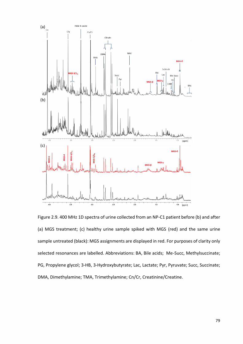
79
Figure 2.9. 400 MHz 1D spectra of urine collected from an NP-C1 patient before (b) and after
(a) MGS treatment; (c) healthy urine sample spiked with MGS (red) and the same urine
sample untreated (black): MGS assignments are displayed in red. For purposes of clarity only
selected resonances are labelled. Abbreviations: BA, Bile acids; Me-Succ, Methylsuccinate;
PG, Propylene glycol; 3-HB, 3-Hydroxybutyrate; Lac, Lactate; Pyr, Pyruvate; Succ, Succinate;
DMA, Dimethylamine; TMA, Trimethylamine; Cn/Cr, Creatinine/Creatine.

80
2.6.3. 1H NMR analysis of urine collected from NP-C1 patients undergoing miglustat
treatment
MGS was detected in urine samples through 1D and 2D NMR techniques, together
with spiking experiments, as previously described. Moreover, valproate, together with its
major metabolite O-acyl-β-glucuronide was detected in 14 of the samples examined in this
cohort. The identity of this metabolite was confirmed by the addition of β-glucuronidase to
urine samples in which the glucuronide adduct was present, and also to untreated samples
serving as negative controls.
β-Glucuronidase equilibration: Urine samples were treated with 400 units of β-
glucuronidase (Sigma–Aldrich, UK) in 0.10 M phosphate buffer (pH 7.00), and then incubated
for a period of 24.0 h. at 37 ◦C prior to 1H NMR analysis.
The shifts experienced by the resonance peaks arising from glucuronate, along with
the appearance of those from the free drug released, revealed the presence of this
metabolite (Figure 2.10). Additionally, MGS, acetaminophen along with its glucuronide and
sulphate metabolites (Figure 2.11), valproate and 1-O-Valproyl-β-glucuronide were
unambiguously identified in urine samples labelled as MGS-treated utilising both 1D and 2D
NMR techniques, despite the structural similarities between the n-alkyl chain moieties in the
structures of MGS, valproate and the latter’s 1-O-valproyl-β-glucuronide metabolite.
Valproate metabolites have been previously identified in urine samples via application of
NMR, i.e. 1H-1H TOCSY and 1H-13C HMBC techniques (178, 179). These results obtained
complemented previous reports which demonstrate that valproate is largely excreted as the
1-O-valproyl-β-glucuronide metabolite (178, 180, 181). Quantification of both MGS and 1-O-

81
valproyl-glucuronide via the integration of their resonances located at the 0.93 - 0.97 and
5.53 - 5.57 ppm buckets respectively is described in detail in the Appendix 1.
Figure 2.10. 400 MHz 1H-1H TOCSY spectrum of urine collected from an NPC1 patient
receiving MGS treatment, before (black) and following (red) equilibration with β-
glucuronidase: 1H NMR signals arising from valproate, the valproate-O-acyl-β-glucuronide
metabolite and MGS are labelled. A typical spectrum is shown.
MGS concentrations in biological fluids have been previously reported in human
plasma and cerebrospinal fluid (CSF) (182), and also mouse plasma (183) by LC-MS/MS.
Lachmann and co-workers quantified MGS using cationic exchange chromatography coupled
with pulsed amperometric detection (184). Treiber et al. investigated the distribution of this

82
agent, after administration in rats, in different tissues and biofluids, including urine, using
HPLC and radiolabeled MGS together with a perbutyrated derivative acting as a prodrug
(185). However, all the techniques mentioned above required previous preprocessing
(separation) steps.
Analytical
technique Preprocessing steps Sample analysed
Run
time LOD Ref
LC-MS/MS SPE Human Plasma <2 min. ca. 60–180 nM (186)
LC-MS/MS
Collection of HPLC fractions, evaporation
(N2) and reconstitution in water followed
by extraction with ethyl acetate.
Human liver
microsomal
samples
6 min. ca. 0.10 nM (187)
UPLC-MS/MS SPE Human Blood 4 min. ca. 600 nM (188)
HPLC-UV
Acidification of samples (pH 4.0) and
extraction with ethyl acetate, followed by
pre-column derivatization with 2,4 -
dibromoacetophenone
Human plasma 15 min.
5 and 0.5 g/ml
for valproate
and 2- propyl-
4-pentenoate
(189)
Table 2.5. Reported methods for valproate and/or its metabolites quantification and
detection in biofluids and tissue: techniques listed along with any further preprocessing
steps and major features of the analysis. Abbreviations: SPE, Solid Phase Extraction; LOD,
Limit Of Detection; Ref, Reference.
The range values of the urinary excretion levels for both MGS and 1-O-valproyl-β-
glucuronide in this patient cohort was 78 - 680 μmol/mmol Cn and 47 - 1154 μmol/mmol Cn
respectively. However, such values are, of course, influenced by differences in the dose of
MGS and valproate administered to the patients involved and by the time-point of urine
sample collection subsequent to dosing, together with any between patient variations in the

83
renal clearance of these agents. Moreover, valproate is mainly excreted as this glucuronide
adduct, although some other metabolites have been found in urine (187); therefore, the
inter-individual variability with regard to valproate biotransformations can be an additional
source of variation. MGS metabolism is still unclear, since it has been reported that 5% MGS
is excreted in urine as a glucuronide adduct (190); however, we could not confirm it in a
recent investigation involving a rat microsomal system and to the best of our knowledge
there are not any reports published with that regard.
As with MGS, previous methods available for the analysis of valproate and its
metabolites in urine include LC-MS/MS (186, 187), together with UPLC-MS/MS (188) and
more conventional HPLC-UV analytical approaches (189) (Table 2.5).
A further advantage of 1H NMR urinalysis is that 1-O-valproyl-β-glucuronide is
particularly sensitive to pH value (i.e., it has a limited hydrolytic stability) and elevated
temperatures (191), and hence the use of techniques which do not require the exposure of
biofluid samples to such methodological stresses is recommended.
Xenometabolome: NMR analysis provides a holistic view of the urine samples
analysed, which permits the exploration of the presence of further resonances arising from
exogenous molecules, such as drugs and their metabolites. These observations encourage
the use of NMR for the resolution of complex mixtures such as biological fluids, where it is
likely to find metabolites from exogenous compounds like drugs, the so called
Xenometabolome (26, 192). The ability of NMR to detect these kind of metabolites will serve
of tremendous aid when dealing with epidemiological studies where patients are likely to be
self-medicated (193), exposed to toxic substances or in cases in which patients undergo dual
or multiple therapies, as notable in the NP-C1 disease cases explored here. It has to be

84
considered that in some countries such as the USA, MGS is not approved, even when this
drug is the only available therapy worldwide, so the risks of self-medicating patients is high.
The biofluid profile of an individual is mainly composed for endogenous metabolites;
nevertheless, the presence of molecules arising from diet or the exposure to hazardous
compounds offers much valuable information to the investigator, since metabolomics
analysis not only reveals the endogenous metabolome, but also how it responds to these
exogenous compounds, and the behaviour of sample donors, e.g. either passively or through
self-administration of medicines and drugs, tobacco and alcohol consumption, etc.
Furthermore, for urine 1H NMR-based metabolomics investigations of NP-C patients,
the assignment of MGS affords valuable information regarding the empirical removal of such
potentially interfering xenobiotic relevant spectral bucket regions prior to conducting such
analyses.
Figure 2.11. Aromatic region from a 1H-NMR 400 MHz urine spectra collected from a NP-C1
MGS-treated patient before (b) and after (a) β-glucuronidase incubation: acetaminophen
aromatic ring C2/6-CH signals are labelled for its different metabolites detectable in urine.
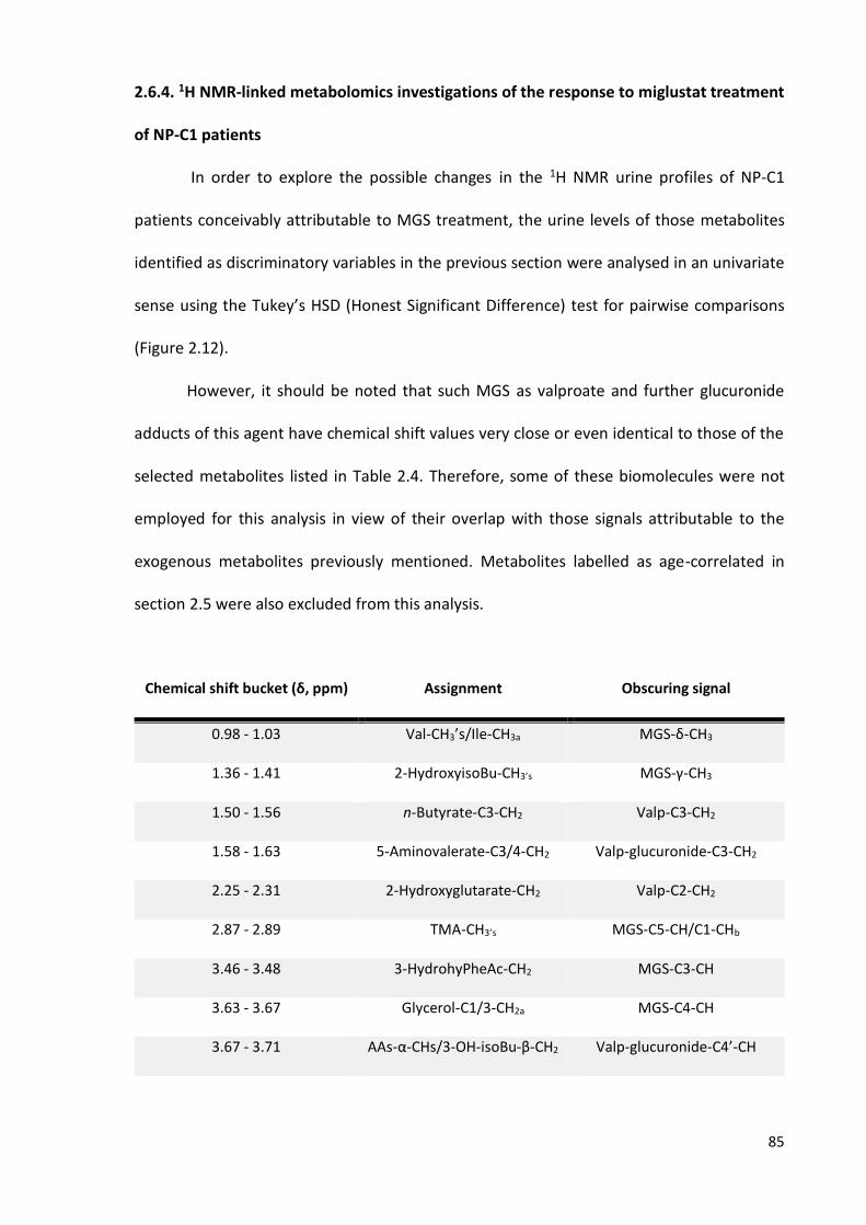
85
2.6.4. 1H NMR-linked metabolomics investigations of the response to miglustat treatment
of NP-C1 patients
In order to explore the possible changes in the 1H NMR urine profiles of NP-C1
patients conceivably attributable to MGS treatment, the urine levels of those metabolites
identified as discriminatory variables in the previous section were analysed in an univariate
sense using the Tukey’s HSD (Honest Significant Difference) test for pairwise comparisons
(Figure 2.12).
However, it should be noted that such MGS as valproate and further glucuronide
adducts of this agent have chemical shift values very close or even identical to those of the
selected metabolites listed in Table 2.4. Therefore, some of these biomolecules were not
employed for this analysis in view of their overlap with those signals attributable to the
exogenous metabolites previously mentioned. Metabolites labelled as age-correlated in
section 2.5 were also excluded from this analysis.
Chemical shift bucket (δ, ppm) Assignment Obscuring signal
0.98 - 1.03 Val-CH3’s/Ile-CH3a MGS-δ-CH3
1.36 - 1.41 2-HydroxyisoBu-CH3’s MGS-γ-CH3
1.50 - 1.56 n-Butyrate-C3-CH2 Valp-C3-CH2
1.58 - 1.63 5-Aminovalerate-C3/4-CH2 Valp-glucuronide-C3-CH2
2.25 - 2.31 2-Hydroxyglutarate-CH2 Valp-C2-CH2
2.87 - 2.89 TMA-CH3’s MGS-C5-CH/C1-CHb
3.46 - 3.48 3-HydrohyPheAc-CH2 MGS-C3-CH
3.63 - 3.67 Glycerol-C1/3-CH2a MGS-C4-CH
3.67 - 3.71 AAs-α-CHs/3-OH-isoBu-β-CH2 Valp-glucuronide-C4’-CH

86
3.88 - 3.92 Hippurate-CH2 Valp-glucuronide-C5’-CH
Table 2.6. List of discriminatory variables with resonances overlapping those arising from
drugs and corresponding metabolites found in urine samples collected from NP-C1 patients
receiving MGS treatment: the exogenous metabolite resonances are listed in the third
column. Chemical shift values employed for assignments are listed in Table 2.3 and Figure
2.10. Abbreviations: 2-HydroxyisoBu-CH3’s, 2-Hydroxybutyrate-CH3’s; 3-HydrohyPheAc, 3-
Hydroxyphenylacetate; AAs, amino acids; 3-OH-isoBu-β-CH2, 3-Hydroxyisobutyrate-β-CH2.
Figure 2.12. Analysis of discriminatory metabolites levels amongst heterozygotes controls
(HET), NP-C1 patients (NPC) and MGS-treated NP-C1 patients (MGS): box plots for
discriminatory variables that represent their normalised intensities for each group

87
(heterozygote, NP-C1 and NP-C1 MGS treated). Statistically significant differences obtained
from the Tukey’s HSD test are indicated by asterisks (p < 0.05, *; p < 0.01, **; p < 0.001, ***).
Abbreviations: BAs, bile acids; 2-OH-3-Me-Bu, 2-Hydroxy-3-methylbutyarte; 3-AIB, 3-
aminoisobutyrate; Cr, creatine. Unknown-1 corresponds to the 0.77 - 0.80 ppm bucket.
Bile acids levels remain the same for NP-C1 and MGS-treated patients, their levels
being higher than those for the HET group, and somewhat lower than that of the NPC group.
As expected, since MGS has no effect on bile acid synthetic pathways, nor cholesterol
metabolism. Additionally, the increase in urinary BAs levels is mainly ascribable to hepatic
problems in NP-C1 patients, and MGS mainly improves their neurologic status, although in
some Gaucher disease patients the hepatomegaly has been partially resolved after MGS
treatment (194, 195).
2-Hydroxy-3-methylbutyrate, 3-AIB, Cr and Gln show similar levels for MGS and HET
groups, being all 4 metabolites correlating with muscle tissue breakdown as will be discussed
in section 6.4.
MGS has been proved to improve the neurological symptoms and concomitantly the
ability of NP-C1 patients to move and walk. Those functions require muscular activation,
which may prevent atrophy, and consequently the release of muscle breakdown products
into the bloodstream, that would be subsequently filtered out into the urine. MGS-treated
NP-C1 patients are usually studied from a functional point of view, focusing in the
neurological symptoms, in which common analysis are ambulation, swallowing, acoustic
response, etc. (115, 196), mainly based in a test originally developed by Iturriaga et al. (197).
Improvements for the majority of these characteristics have been observed after MGS
treatment. Therefore, an increase in patients mobility triggered by an improvement in their

88
neurological status caused by MGS treatment would explain these results. Nevertheless,
these outcomes might contrast with some well-known adverse effects of MGS treatment as
diarrhoea and weight loss (198, 199); however, diarrhoea is directly related to the loss of
liquids and the body weight is usually recovered after 24 months of treatment (199, 200).
Both issues have their source in gastrointestinal problems caused for the intake of this drug
and not in endogenous protein degradation.
Higher N-acetylated metabolites levels in urine is a common feature of some LSD
such as Sandhoff and Tay-Sachs diseases. These biomolecules are mainly gangliosides, the
degradation pathway of which is affected by mutations in one of the catabolic enzymes
involved. Indeed, the accumulation of gangliosides in the brain is the cause of some of the
neurological symptoms occurring in NP-C1 patients (201, 202). The presence of these N-
acetylated biomolecules can be monitored by 1H NMR analysis of urine (203). The 2.02 - 2.08
ppm bucket was selected by CCR-LDA and ranked 10th, showing higher levels for the NPC
group (p = 2.15 x 10⁻², FC = 1.25). The well-known effects of MGS in reducing
glycosphingolipid concentrations in brain can lead to the significant decrease observed in
this study for urinary N-acetyl-metabolites in NP-C1 patients undergoing MGS treatment.
Indeed, investigations conducted with animal models of Tay-Sachs and Sandhoff under MGS
treatment revealed the delayed accumulation of GM2 ganglioside in the brain (149, 204).
Methanol levels, despite experiencing a slightly increase with regard to NPC group,
remain significatively lower than the HET group. Hence, MGS has no effect on this
metabolite. The absence of more resonances available arising from bacterial metabolites
prevent generalisation of the effect of MGS on microbiota activity/population in NP-C1
disease.

89
Quinolinate (QUIN) levels are significantly lower for the MGS-treated group than for
the NPC one, showing a similar pattern to HET participants. Since the source of this
metabolite is somewhat unclear (macrophages infiltrate, imbalance in NAD+/NADH
synthesis, muscle wasting, etc.), the results observed here are difficult to attribute to a
specific physiological change caused by MGS treatment. Nevertheless, recent studies
suggest that the inflammation process associated to the NP-C pathophysiology is secondary
to the tissue damage, so it is a response from the body to fight back the disease (205); and
therefore, as MGS corrects some of the symptoms arising from the disease process, then the
lower levels of QUIN may reflect the reduced inflammatory process as an indirect
consequence of the treatment.

90
CHAPTER 3
1H NMR LINKED METABOLOMICS ANALYSIS OF
PLASMA SAMPLES COLLECTED FROM NP-C1
PATIENTS, HETEROZYGOUS CARRIERS, HEALTHY
PARTICIPANTS AND MIGLUSTAT TREATED NP-C1
PATIENTS
3.1. PLASMA SAMPLES COLLECTION AND PREPARATION FOR NMR ANALYSIS
75 plasma samples collected from NP-C1 patients, 89 from MGS treated NP-C1
patients, 31 from heterozygous carriers and 30 collected from healthy participants (as
controls) were stored at -80◦C. NP-C1 patients untreated and MGS treated together with
heterozygotes were fasted prior to sample collection. However, healthy participants were
not fasted. Plasma was separated from whole-blood using a histopaque column (gradient
density column). Samples were thawed on ice and centrifuged for 3.0 min. at 850 x g. 200 μL
of plasma was diluted with 300 μL Mili-Q H2O and 55 μL D2O (the latter to provide an NMR
field frequency lock). Samples were transferred to standard 5 mm-diameter NMR tubes
(Norell, UK) for analysis.

91
Disease class NPC MGS HET WT
Number (male/female) 75 (42/33) 89 (54 /35) 31 ( 15/13)* 30 (23/6)
Average age in years (range) 19 (0.3 - 54) 11 (1 – 28) N/A ~15 (0.4 - 18)**
Table 3.1. Participants’ information included in the NP-C1 plasma dataset: Abbreviations:
NPC, NP-C1 disease patients; MGS, NP-C1 patients undergoing miglustat treatment; HET,
heterozygous carriers; WT, healthy participants. *Information relative to the gender of some
heterozygous carriers was not available; **, the age of all healthy participants was not
available.
3.2. NMR ANALYSIS OF PLASMA PROFILES
NMR spectral acquisition was performed on a Bruker AVIII 700 spectrometer
equipped with a 1H (13C/15N) TCI cryoprobe (Department of Chemistry, University of Oxford)
with sample temperature stabilised at 310K. 1H NMR spectra were acquired using a 1D
NOESY presaturation (noesygppr1d pulse sequence, Bruker) scheme for attenuation of the
water resonance with 2 s presaturation. Low molecular weight metabolite spectra were
acquired using a spin-echo sequence [Carr-Purcell-Meiboom-Gill (CPMG)] with presaturation
for water suppression (cpmgpr1d pulse sequence, Bruker) with a τ interval of 0.39 ms, 80
loops, and echo time of 0.40 ms, 32 scans, an acquisition time of 1.46 s, a relaxation delay of
2 s, and a fixed receiver gain.
3.2.1. 1H NMR plasma profiles of NP-C1 patients
1H NMR resonances were assigned on the basis of chemical shifts, coupling constants
and literature values (46, 206, 207). Spectra acquired from plasma samples contained
92
different resonance signals ascribable to amino acid, small organic acid anions, glucose,
lipoproteins and glycoproteins. Additionally, some other signals from exogenous agents
were observed in the NMR spectra such as Ca-EDTA2- and Mg-EDTA2- complexes resonances
arising from the chelation of these metal ions by this agent, which was present in the sample
collection tubes as an anticoagulant (Figure 3.2); resonances arising from the plasma
separation procedure can also be observed in the spectrum such as a singlet at 2.26 ppm
and signals around 1.80 ppm. Broad resonances from 3.40 to 4.45 ppm and from 5.40 to 5.62
ppm are attributable to the polymer (polysucrose-based) contained in the histopaque
column employed for plasma isolation (Figure 3.1).
Histopaque is a method employed to separate the different phases present in blood,
i.e. those conformed by plasma from that containing lymphocytes, monocytes and platelets,
and an additional phase conformed of granulocytes and erythrocytes, through a density
gradient media composed of polysucrose, which is the broad signal observed in Figure 3.1,
in 3.40 - 4.45 and 5.40 - 5.62 ppm NMR spectral regions. This solution incorporates sodium
diatrizoate, observable as a singlet at 2.26 ppm. Additional signals were found after running
a sample of water, as control, ca. 1.80 ppm, which probably arises from the histopaque
treatment of blood samples. In view of the exogenous NMR-visible signals assignable to the
sucrose polymer and further agents derived from histopaque treatment that overlayed some
resonance signals of biological interest, this plasma isolation method presents limitations for
NMR-based metabolomics studies.

93
Figure 3.1. Stack plot of (a) a plasma sample separated by histopaque and (b) a water
sample also passed through a histopaque column.
The usual methods employed to avoid anticoagulation during blood sample
collection include the usage of sample tubes containing lithium-heparin, citrate or the
sodium salt of EDTA. Both citrate and EDTA give 1H NMR-visible resonance peaks in plasma
spectra, subsequently acquired, at the concentrations typically used (208), whilst plasma
samples collected in heparin-Li+ present only a weak and broad spectrum that can be
removed through CPMG pulse sequences for spectral acquisition. However, the presence of
EDTA signals in the 1H NMR plasma spectra could offer additional information, since the
resulting Ca and Mg-EDTA2- resonances are clearly observable, and can be employed to
monitor both metal ions. Although other metal ions (Zn2+) could be interfering in the complex
equilibrium that involves Ca-EDTA2-:Ca2+:Mg-EDTA2-:Mg2+:Free-EDTA. Barton et al. (209)
explored the influence of the differing anticoagulants noted above on NMR metabolomics
plasma investigations, and concluded that only a few resonances are completely masked by
EDTA and EDTA-metal ions resonances, such as acetylcarnitine-N(CH3)3 resonance at 3.60
ppm (Ca-EDTA2--N-CH2CH2-N- peak), carnitine resonances at ca. 3.21 ppm (free EDTA-N-CH2-
CO- peak), ornithine-C4-CH2 resonances at 3.07 ppm (Ca-EDTA2--N-CH2CH2-N- peak) and cis-

94
aconitate-CH2 resonance at 3.44 ppm (Ca-EDTA2--N-CH2CH2-N- peak). Their final conclusion
was that NMR metabolomics investigations utilising plasma samples collected in EDTA tubes
can be conducted without any major drawbacks.
Figure 3.2. (a) 0.75 - 4.45 and (expansion of the BCAA region is included as an insert) (b) 5.10
- 8.50 ppm regions from an NP-C1 patient 1H NMR plasma profile: 1, CH3-VLDL/LDL; 2,-(CH2)n-
VLDL/LDL; 3, Lactate-CH3; 4, Alanine-CH3; 5, TG-CH2CH2CO; 6, Arginine-C4-CH2; 7, Lysine-C5-
CH2; 8, Arginine-C3-CH2; 9, Acetate-CH3; 10, CH2CH2CH=-; 11, N-acetyl-glycoprotein-CH3; 12,
95
Proline-1; 13, Glutamate-C2-CH2; 14, Pyruvate-CH3; 15, Glutamate-C3-CH2; 16, Glutamine-
C4-CH2; 17, Citrate-CH2a; 18, Creatine-CH2; 19, TMAO-CH3’s; 20, Proline-2; 21,
Phosphocholine-NCH3; 22, Lactate-CH; 23, =C-CH2-C=, -CH=CH-; 24, Tyrosine-C3/5-CH; 25,
Histidine-C5-CH; 26, Tyrosine-C4/6-CH; 27/28-Phenylalanine; 29, Histidine-C6-CH; 30,
Formate-H.
3.3. DATA PREPROCESSING
Any resonances arising from histopaque contamination, i.e., the 1.80 - 1.86, 2.18 -
2.31, 3.30 - 4.50, and 5.37 - 5.68 ppm spectral regions were removed. Additionally, the 1.15
- 1.17 ppm region was excluded in view of ethanol contamination, likely as a result of skin
disinfection prior to sample collection. Regions containing only noise across all spectra were
also excluded, so that a dataset containing 38 columns (variables) and 252 rows (samples)
was obtained. Prior to any statistical analysis, the whole dataset was sum-normalised, Pareto
scaled and cube-root transformed.
3.4. UNIVARIATE AND MULTIVARIATE ANALYSIS OF THE 1H NMR PLASMA DATASET
3.4.1. Univariate data analysis: Tukey’s HSD test
Since some information concerning the age and gender of participants was not
available, an ANOVA/ANCOVA model similar to those employed in previous and next
sections cannot be accurately employed. However, a post-hoc Tukey’s range test (honest
significant test, HSD) was applied to the sum-normalised, cube-root transformed and Pareto-
scaled plasma dataset. Those variables selected by the RFs technique as discriminatory

96
features are supplemented in Table 3.3 by a ‛*’ sign to indicate the level of significance based
on their 1H NMR plasma profiles.
3.4.2. Multivariate data analysis
3.4.2.1. Preliminary analysis: PCA
PCA scores plots illustrated in Figure 3.2 reveal that WT is the most distinct
classification group, since a clear cluster can be observed when plotted against the NPC, HET
and MGS groups. However, the HET and NPC groups do not form clear clusterings in the
scores plot, and hence there is no separation between these groups. The influence of
miglustat (MGS) treatment on the 1H NMR plasma profiles of NP-C1 patients was also
explored. Scores plot of PC1 vs. PC2 in Figure 3.3 did not show any differences between both
groups (MGS vs. NPC). Indeed, apart from WT, the MGS plasma profiles were found to be
very similar to the remaining disease classification groups (NPC and HET).
3.4.2.2. Classification performance
Random Forests (RFs): The procedure described in section 2.4.3 for RFs analysis was
also employed for the plasma dataset. Since in this case the number of groups is 4, this
analysis was applied for each pair of different groups, with the exception of MGS vs. HET
one, since that comparison was irrelevant for this study (Table 3.2) as heterozygous carriers
do not present any symptomatology associated to NP-C1 disease, and therefore, they are
not treated with MGS.

97
(a) (b)
(c) (d)
OOB error Accuracy
Disease class WT NPC Disease class WT NPC
NPC 0.106 (0.003) NPC 0.904 (0.005)
HET 0.175 (0.005) 0.226 (0.003) HET 0.818 (0.007) 0.765 (0.007)
MGS 0.160 (0.003) 0.353 (0.004) MGS 0.832 (0.006) 0.646 (0.006)
Sensitivity Specificity
Disease class WT NPC Disease class WT NPC
NPC 0.926 (0.005) NPC 0.853 (0.011)
HET 0.824 (0.011) 0.754 (0.020) HET 0.823 (0.012) 0.778 (0.007)
MGS 0.864 (0.007) 0.664 (0.008) MGS 0.729 (0.015) 0.632 (0.010)
Table 3.2. RF classification performance for all 4 groups analysed in the plasma dataset:
tables showing mean and SEM values (the latter between brackets) for OOB error (a),
accuracy (b), sensitivity (c) and specificity (d) values.
It should be noted that accuracy, sensitivity and specificity show lower values for the
HET vs. NPC classification comparison, and even lower values for MGS vs. NPC one (Table
3.2), and this confirms the absence of differences between the 1H NMR profiles of the HET
and NPC groups, and the unaltered profile of NP-C1 patients despite of being under MGS
treatment. However, the remaining group pair comparisons were successfully classified by
RFs as illustrated in the multidimensional scaling plots shown in Figure 3.3, where the
classification of the test set is exhibited.
The RFs performance on WT vs. NPC groups resulted in an OOB error value of 0.106
± 0.003 (mean ± SEM), which reveals a successful classification of the training set. The
multidimensional scaling plot of the proximity matrix calculated from one of the RFs
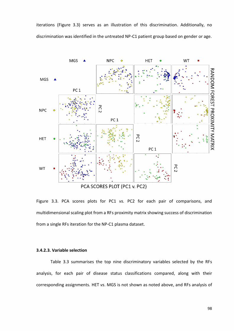
98
iterations (Figure 3.3) serves as an illustration of this discrimination. Additionally, no
discrimination was identified in the untreated NP-C1 patient group based on gender or age.
Figure 3.3. PCA scores plots for PC1 vs. PC2 for each pair of comparisons, and
multidimensional scaling plot from a RFs proximity matrix showing success of discrimination
from a single RFs iteration for the NP-C1 plasma dataset.
3.4.2.3. Variable selection
Table 3.3 summarises the top nine discriminatory variables selected by the RFs
analysis, for each pair of disease status classifications compared, along with their
corresponding assignments. HET vs. MGS is not shown as noted above, and RFs analysis of

99
the NPC vs. MGS comparison did not show any classification success, and therefore no
ranking was extracted from that analysis.
Bucket
(ppm) Assignment
Multiplicity
(J, Hz)
NPC vs.
WT
HET vs.
WT
MGS vs.
WT
NPC vs.
HET
0.81 - 0.83 HDL-CH3 br ↓**(2)
0.83 - 0.89 VLDL-CH3 br ↑***(6) ↑***(2) ↑***(6)
0.89 - 0.95 Isoleucine-C5-CH3 t (7.3) ↑***(9) ↑*(9)
1.13 - 1.15 2,3-butanediol-(CH3)2 d (6.1) ↑(9)
1.21 - 1.23 HDL-(CH2)n br ↑***(7) ↑(8)
1.23 - 1.25 LDL-(CH2)n br ↑***(5) ↑***(3) ↑***(4)
1.25 - 1.31 VLDL-(CH2)n br ↑***(2) ↑***(5) ↑***(1) ↑*(7)
1.31 - 1.37 Lactate-CH3 d (6.8) ↑***(7) ↑***(7)
1.53 - 1.61 -CH2CH2CO br ↑***(1) ↑**(8) ↑***(3) ↑** (3)
1.94 - 1.96 Proline 1 m ↑***(9)
1.96 - 1.98 Proline 2 m ↑***(6)
2.03 - 2.09 N-acetylglycoprotein/CH2-CH2-CH= s/br ↑***(8)
2.52 - 2.58 Ca-EDTA s ↑***(8) ↑***(1)
5.26 - 5.32 Unsaturated lipid 2 br ↑***(3) ↑***(1) ↑***(2)
5.32 - 5.37 Unsaturated lipid 1 br ↑***(4) ↑***(4) ↑***(5) ↓ (5)
7.02 - 7.08 Histidine-C2-CH s ↑*(6)
7.74 - 7.85 Histidine-C5-CH s ↓*(4)
Table 3.3. RFs discriminatory variables for the NP-C1 plasma dataset: Arrows indicate an
increase/decrease in the measured metabolite with respect to the WT samples (or with
respect to the HET samples in the case of the NPC vs. HET comparison). The results of the
Tukey’s HSD test for each metabolite identified by RFs analysis are indicated by asterisks (p
< 0.05, *; p < 0.01, **; p < 0.001, ***). The RFs ranking is based on their MDA value, and is

100
represented in brackets. Unsaturated lipid 1 and 2 refer to =C-CH2-C= and -CH=CH- protons
respectively.
Since some of the variables listed in Table 3.3 were highlighted in more than one
classification comparison as discriminant features, their levels are then illustrated as box
plots in Figure 3.5.
3.4.2.4. ROC curve analysis
In order to seek those variables that more efficiently contribute to the classification
of NP-C1 patients when compared to healthy control ones, a ROC curve analysis was
performed including WT and NPC classes using RFs as a tool for classification. Metabolites
selected as important features for discrimination listed in Table 3.3 were employed for this
analysis.
The majority of variables selected for classification for the NPC vs. WT comparison
were assignable to lipoprotein-associated TGs, being actually able to successfully classify the
WT and NPC groups with only 2 variables [AUC (mean) = 0.912; range, 0.772 - 0.982].
Isoleucine (Ile) and lactate were also included in the models, being selected in ca. 86% of
those constructed [Figure 3.4 (b)].

101
Figure 3.4. (a) ROC curves and (b) bubble diagram for variable importance for the NP-C1
blood plasma dataset: different combinations of variables gave different AUC values, ranging
from 0.912 for 2 variables, and up to 0.946 with 9 variables, as indicated in the Table inserted
in (a). (b) Variable rankings arising from ROC analysis (depicted in the vertical axis in); blue
bubbles indicate metabolites with lower levels in the NPC group, and orange ones those with
higher levels. The size of each bubble is correlated with the fold change (FC). Abbreviations:
N-AGP, N-acetylglycoproteins; TPR, True Positive Rate; FPR, False Positive Rate.
3.5. 1H NMR PLASMA PROFILES OF NP-C1 PATIENTS, HETROZYGOUS CARRIERS, HEALTHY
PARTICIPANTS AND MIGLUSTAT TREATED NP-C1 PATIENTS
Fasting at least 8 hours prior to lipid determination in blood or plasma is a common
requirement in order to prevent increased lipid levels ascribable to food intake, specifically
TGs. Although samples collected from healthy participants are not fasting samples, levels of
several lipidic species for NPC, HET and MGS groups are higher than those for this WT group

102
(Figure 3.5) and recent studies have reported only a low correlation between fasting times
and plasma lipid levels (210). However, the results shown herein present some limitations.
Figure 3.5. Box plots for metabolites selected in more than one classification problem for the
NP-C1 plasma dataset: those metabolites selected by the RFs models and also showing
significant differences are indicated by asterisks (p < 0.05, *; p < 0.01, **; p < 0.001, ***).
NP-C1 is a disorder mainly affecting lipid and cholesterol trafficking. Table 3.3 reveals
that differences in such lipid resonances were selected as important features for
103
discrimination between untreated NPC patients and the WT participants. Most notably, NP-
C1 patients exhibit an increase in both VLDL lipid signals [i.e. VLDL-CH3 and VLDL-(CH2)n-],
LDL-(CH2)n-, HDL-(CH2)n-, lipid -CH2CH2CO, and vinylic TGs spectral regions. In addition,
lactate is significantly increased for all the groups when expressed relative to the WT one.
The N-acetylglycoproteins and lactate spectral regions were also highlighted as important
variables for discrimination in view of their higher levels in the NP-C1 group.
The MGS group’s 1H NMR plasma profiles show a very similar pattern to the NPC one
for those spectral regions assignable to lipids, except for the -CH2CH2CO and unsaturated
lipids-1, for which the MGS group has lower levels (Table 3.3). Interestingly, the isoleucine
bucket was neither selected as a discriminatory variable for MGS-treated samples, nor did it
attain any statistical significance (showing very similar levels to the NPC group). However,
some additional variables were required for discrimination between MGS-treated patients
and the healthy controls (WT group), including increases in the Ca-EDTA2- and 2,3-butanediol
buckets.
The HET group exhibited an intermediary phenotype for plasma lipoproteins
between the MGS/NPC and WT ones, since the pattern for VLDL-CH3, Ile, VLDL-(CH2)n-, TG-
CH2CH2CO and unsaturated lipid-1 in the 1H NMR plasma spectra is NPC > MGS > HET >> WT,
similar to WT although the unsaturated lipid 2 resonance signal is of higher intensity than
that of the MGS group. Similar to the NP-C1 patients, the key variables responsible for
discrimination between the HET and WT groups are dominated by lipid resonances. Two
variables responsible for discrimination between NPC and control spectra were not
identified in the HET vs. WT analysis (N-acetyl glycoprotein/CH2-CH2-CH= and lactate), whilst
an increase in proline resonances is observed only for the HET samples. This HET group was
successfully classified when compared to the WT one, but the profiles exhibited were closer

104
to the NPC group; RFs analysis for this pair (HET vs. NPC) of groups gave fair values for
accuracy, specificity and sensitivity. Additionally, both histidine buckets contributed to the
discrimination between the NPC and HET classes, this being the only case in which this amino
acid resonances were featured as discriminatory variables.
These similarities between the HET and NPC groups are somewhat surprising, since
heterozygous carriers do not manifest any pathological symptoms, and this may indicate an
irrelevant role of lipoprotein metabolism in the disease process.
105
CHAPTER 4
1H NMR LINKED METABOLOMICS ANALYSIS OF
LIVER SAMPLES COLLECTED FROM AN NP-C1
MOUSE MODEL
4.1. LIVER AQUOEUS METABOLITES EXTRACTION FOR NMR ANALYSIS
NP-C1 mutant (BALB/cNctr-Npc1m1N/J, Npc1-/-; NP-C1), control (Npc1+/+; WT) and
NP-C1 heterozygous mice (Npc1+/-; HET), were generated from heterozygote matings and
the genotype of offspring was determined by polymerase chain reaction (PCR), as described
previously (211). Mice were bred and housed under standard non-sterile conditions at the
University of Oxford. All animal procedures were conducted using protocols approved by the
UK Animals (Scientific Procedures) Act (1986). In total, 65 liver samples from gender-
matched heterozygous carrier (HET), NP-C1 disease (NPC) and wild type (WT) mice were
collected at 3, 6, 9 and 11 weeks.

106
Collection Time Point (weeks)
Disease Class 3 6 9 11
Wild type (WT) 4 (3/1) 3 (0/3) 7 (5/2) 8 (5/3)
Heterozygotes (HET) 0 (0/0) 0 (0/0) 9 (5/4) 10 (5/5)
NP-C1 (NPC) 4 (2/2) 6 (4/2) 11 (6/5) 3 (0/3)
Number (male/female)
Table 4.1. Liver samples available for 1H NMR-linked metabolomics analysis at time-points of
3, 6, 9 and 11 weeks.
Aqueous metabolites extraction for NMR analysis: The extraction protocol
employed was based on the procedure described by Waters et al. (212) with slight
modifications. A portion of hepatic tissue (ca. 80 mg) was taken, for each piece of liver 0.02
mL of ice-cold extraction solvent (H2O/CH3CN, 1:1) per mg of tissue were added. The sample
was then mechanically homogenized using an electric pestle rotor (Sigma-Aldrich UK, UK).
The homogenates were centrifuged at 10,000 × g for 10 min at 4 °C. Supernatants
(hydrophilic metabolites) were freeze-dried and reconstituted in 500 µL of D2O containing
0.05 % wt. TSP, and 50 µL of pH 7 phosphate buffer to reach a final concentration of 0.01 M,
then vortexed and centrifuged at 5,000 x g for 10 min. at room temperature. Supernatants
were transferred into 5-mm NMR glass tubes (Norell, UK) for NMR analysis.
4.2. NMR ANALYSIS OF LIVER EXTRACTS
1D 1H NMR: Single-pulse 1H NMR spectra experiments were carried out on a Bruker
Avance AM-400 spectrometer (Leicester School of Pharmacy facility, DMU, Leicester, UK)
operating at a frequency of 399.94 MHz and a probe temperature of 298 K. Spectra were

107
acquired using noesygppr1d (Bruker) pulse sequence for water suppression. For each
spectrum 128 scans were acquired, a relaxation delay of 3 s, spectral width of 4,800 Hz and
a time domain of 32 K points. Spectra were acquired in an automated manner using a sample
changer for continuous sample delivery.
1H-1H COSY: This experiment was carried out at 27 °C on a Bruker AV 400 MHz
(Leicester School of Pharmacy, DMU, Leicester, UK) using the same parameters as those
delineated above for urine samples.
13C-1H HSQC: Heteronuclear Single Quantum Coherence (HSQC) spectra were
acquired on a Bruker Avance AM-400 spectrometer (Leicester School of Pharmacy, DMU,
Leicester, UK). For the HSQC experiments, hsqcedetgpsp.3 pulse sequence (Bruker) was
employed, and 256 scans for 128 increments were acquired for each spectrum. The F2 and
F1 spectral widths were 6,340 and 16,600 Hz, respectively.
4.2.1. 1H NMR hepatic profiles of NP-C1 mice
Typical 400 MHz single-pulse 1H NMR spectra of liver samples (Figure 4.1) collected
from NP-C1 disease mice and their heterozygous carrier, plus wild type specimens controls
contained a large number of different types of polar low molecular weight metabolites,
including amino acids [alanine (Ala), isoleucine (Ile), lysine (Lys), tyrosine (Tyr), phenylalanine
(Phe)] and derivatives such as sarcosine, small organic acids (2-aminobutyrate, 2-
hydroxybutyrate, lactate), carbohydrates (glucose, glycogen), nucleotides (GMP,GTP), etc.
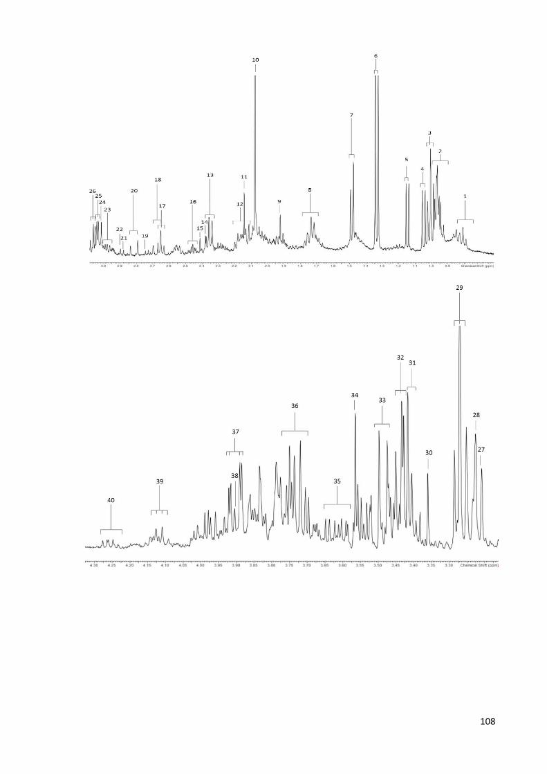
108
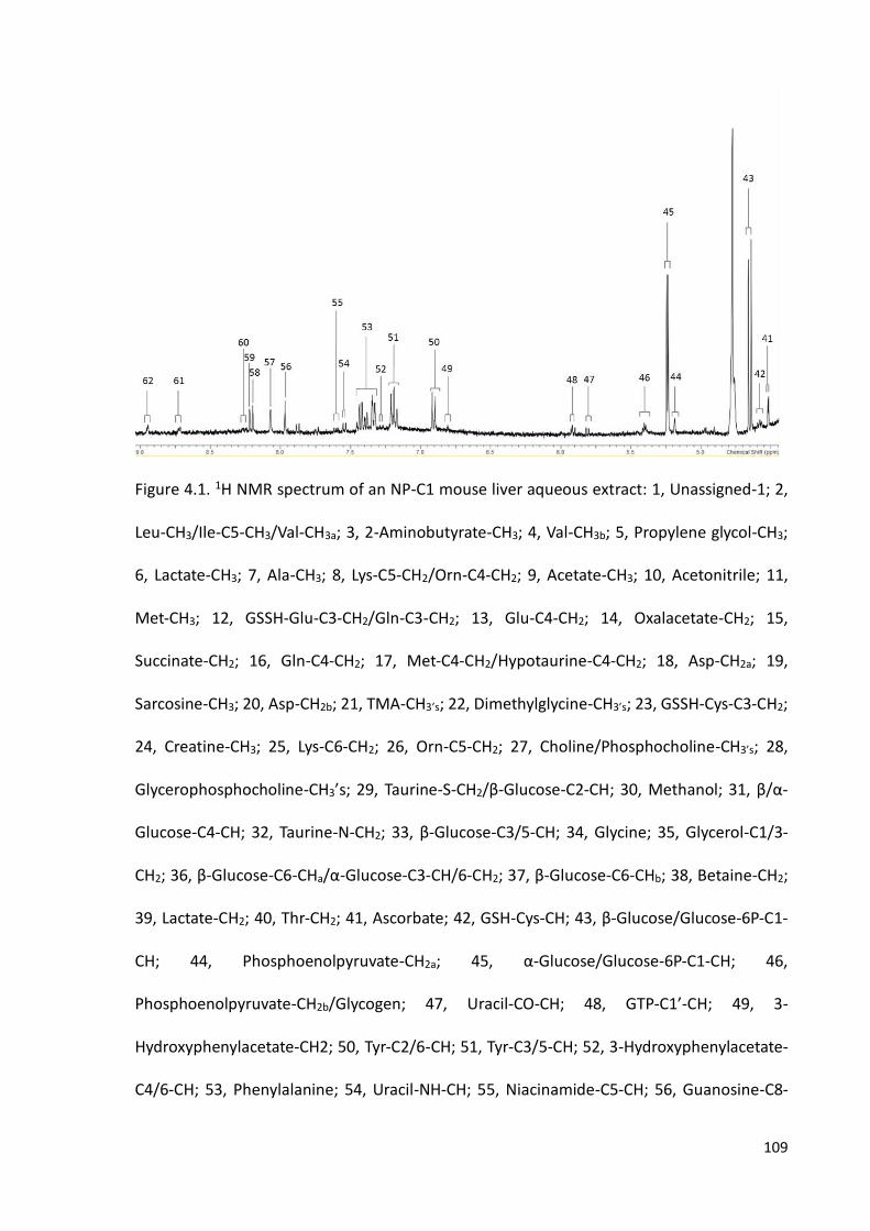
109
Figure 4.1. 1H NMR spectrum of an NP-C1 mouse liver aqueous extract: 1, Unassigned-1; 2,
Leu-CH3/Ile-C5-CH3/Val-CH3a; 3, 2-Aminobutyrate-CH3; 4, Val-CH3b; 5, Propylene glycol-CH3;
6, Lactate-CH3; 7, Ala-CH3; 8, Lys-C5-CH2/Orn-C4-CH2; 9, Acetate-CH3; 10, Acetonitrile; 11,
Met-CH3; 12, GSSH-Glu-C3-CH2/Gln-C3-CH2; 13, Glu-C4-CH2; 14, Oxalacetate-CH2; 15,
Succinate-CH2; 16, Gln-C4-CH2; 17, Met-C4-CH2/Hypotaurine-C4-CH2; 18, Asp-CH2a; 19,
Sarcosine-CH3; 20, Asp-CH2b; 21, TMA-CH3’s; 22, Dimethylglycine-CH3’s; 23, GSSH-Cys-C3-CH2;
24, Creatine-CH3; 25, Lys-C6-CH2; 26, Orn-C5-CH2; 27, Choline/Phosphocholine-CH3’s; 28,
Glycerophosphocholine-CH3’s; 29, Taurine-S-CH2/β-Glucose-C2-CH; 30, Methanol; 31, β/α-
Glucose-C4-CH; 32, Taurine-N-CH2; 33, β-Glucose-C3/5-CH; 34, Glycine; 35, Glycerol-C1/3-
CH2; 36, β-Glucose-C6-CHa/α-Glucose-C3-CH/6-CH2; 37, β-Glucose-C6-CHb; 38, Betaine-CH2;
39, Lactate-CH2; 40, Thr-CH2; 41, Ascorbate; 42, GSH-Cys-CH; 43, β-Glucose/Glucose-6P-C1-
CH; 44, Phosphoenolpyruvate-CH2a; 45, α-Glucose/Glucose-6P-C1-CH; 46,
Phosphoenolpyruvate-CH2b/Glycogen; 47, Uracil-CO-CH; 48, GTP-C1’-CH; 49, 3-
Hydroxyphenylacetate-CH2; 50, Tyr-C2/6-CH; 51, Tyr-C3/5-CH; 52, 3-Hydroxyphenylacetate-
C4/6-CH; 53, Phenylalanine; 54, Uracil-NH-CH; 55, Niacinamide-C5-CH; 56, Guanosine-C8-

110
CH; 57, GTP/GMP-C8-CH; 58, GMP-C8-CH/Hypoxanthyne-C2-CH; 59, Hypoxanthine-C8-CH;
60, Nicotinate-C4-CH; 61, Nicotinate/Niacinamide-C6-CH; 62, Nicotinate/Niacinamide-C2-
CH.
4.3. DATA PREPROCESSING
After 1D spectral acquisition, an LB = 0.30 Hz was applied to all spectra prior FT and
subsequent baseline and phase corrections were carried out using NMR Spectrus processor.
The intelligent bucketing procedure applied gave a dataset of 65 rows (samples) and 207
columns (variables). The integral intensity values for each bucket were normalised and
referenced to the TSP signal (s, δ = 0.00 ppm). Spectral regions which did not contain any
resonances were removed, so that a final dataset of 65 samples x 143 variables was obtained
for further analysis.
Prior to further analysis, NMR spectra were visually checked for any major
disturbances. None of the spectra was excluded for subsequent statistical analysis.
4.4. UNIVARIATE AND MULTIVARIATE ANALYSIS OF THE 1H NMR MURINE HEPATIC
DATASET
4.4.1. Univariate data analysis: ANCOVA
The experimental design for univariate analysis of the 1H NMR buckets from the NP-
C1 liver dataset involved an ANCOVA model that incorporates 3 factors and 6 primary
sources of variation: (1) ‛between-disease classifications’ (qualitative NPC disease-active vs.
the combined HET/WT control group), fixed effect (Di); (2) ‛between-genders’ fixed effect
(qualitative) ‛nested’ within ‛disease classifications’ (Gj); (3) experimental sampling time-

111
point fixed effect (quantitative, Tk); (4, 5 and 6) disease classification x gender, disease
classification x time-point and gender x time-point first-order interaction components (DGij,
DTik and GTjk) respectively. This experimental design is represented by Equation 20, in which
Yijk represents the (univariate) predictor variable value observed, μ its overall population
mean value in the absence of any significant, influential sources of variation, and e ijk the
unexplained error (residual) contribution.
Yijk = μ + Di + Gj + Tk + DGij + DTik + GTjk + eijk (20)
4.4.2. Multivariate data analysis
4.4.2.1. Preliminary analysis: PCA
PCA was employed in order to explore any clustering present within the data
regarding the 3 groups initially studied. PCA analysis revealed that there was a significant
clustering of the NP-C1 disease classification which was distinct from both the HET and WT
groups; however, no discrimination between the latter two disease status classifications was
found. Indeed, PC 4 vs. PC 3 vs. PC 2 score plot obtained with the unsupervised PCA approach
(Figure 4.2) provided the best visualisation of this NPC vs. the combined HET/WT group
discrimination. The NPC cluster exhibited significantly higher and lower scores vectors than
those of the combined HET/WT ones for components 2 and 4 respectively; there appeared
to be no ‘between-classification’ differences between these scores vectors for component 3
as can be observed in the projections of the 3D plot on the 2D planes.

112
Figure 4.2. (a) Three-Dimensional (3D) PC4 vs. PC3 vs. PC2 scores plot arising from PCA of the
liver NP-C1 dataset (yellow diamonds, NPC; red squares, WT; green circles, HET). (b)
Multidimensional scaling plot of a random forests proximity matrix from HET/WT vs. NPC
analysis: this plot demonstrates the success of discrimination from a single RFs iteration.
4.4.2.2. Classification performance
Random Forests (RFs): The RFs classification methodology for these liver samples
was performed in the same way as described previously for the urinary and plasma datasets,
but in this case the RFs tuning gave optimised values of 1,000 for the number of trees and
12 variables selected at each split. Initially, 3 groups were analysed using RFs: HET, WT and
NPC mice. RFs performed on HET vs. WT gave OOB = 0.428, meaning a 57.2% out of sample
accuracy. However, lower values for OOB error were obtained when RFs was employed with
NPC vs. HET (OOB = 0.175) and NPC vs. WT (OOB = 0.190). In view of this situation, HET and
WT were merged in one group (HET/WT) for further analysis. This analysis gave OOB error
mean values of 0.190 ± 0.00041. For prediction performance, the values for sensitivity,
specificity and accuracy were 0.799 ± 0.0013, 0.843 ± 0.0034 and 0.810 ± 0.00084

113
respectively. A plot representing the classification performance of RFs for the test set is
depicted in Figure 4.2 (b).
4.4.2.3. Variable selection
The variable importance values for the 143 variables were computed in the same way
as previous datasets (urine and plasma) using the mean decrease accuracy value (MDA). This
value is computed from permuting OOB data, so that for each tree the prediction error on
the OOB portion of the data is recorded as an error rate for classification. Subsequently, the
procedure is repeated after permuting each feature. The difference is then averaged over
the ensemble of trees, and normalized by the standard deviation of the differences (165).
The top 15 variables, together with their respective ranking, p-values and assignments are
presented in Table 4.2.
Variable
Ranking
Bucket
(ppm) Assignment Multiplicity
ANCOVA p-value
for disease Fold change
1 7.30 - 7.35 Phenylalanine-C1/C2-CH d (6.8) 1.60 x 10⁻⁴ +1.56
2 7.17 - 7.23 Tyrosine-C3/C5-CH d (8.6) 1.70 x 10⁻⁴ +1.38
3 6.88 - 6.93 Tyrosine-C2/C6-CH d (8.2) 1.45 x 10⁻³ +2.25
4 8.92 - 8.97 Nicotinate-C2-CH d (2.1) 1.30 x 10⁻³ -1.49
5 2.99 - 3.05 Lysine-C6-CH2/Ornithine-C5-CH2 t/t 2.00 x 10⁻⁴ +1.51
6 2.62 - 2.67 Hypotaurine-C4-CH2SO2-/Methionine-C4-CH2
m 2.40 x 10⁻³ +1.96
7 6.78 - 6.81 3-Hydroxyphenylacetate-C4-CH m 3.80 x 10⁻⁴ -3.45
8 0.94 - 0.99 Valine-CH3 d (7.1) 1.49 x 10⁻² +1.35
9 4.24 - 4.27 Threonine-C3-CH m 3.40 x 10⁻⁴ +1.30
10 8.69 - 8.74 Niacinamide-C6-CH dd (4.4, 1.7) 0.26 -1.01
11 8.23 - 8.29 Nicotinate/Niacinamide-C4-CH m/dd 8.11 x 10⁻² -1.37

114
12 7.35 - 7.41 Phenylalanine-C3/4/5-CH m 1.22 x 10⁻² +3.21
13 0.77 - 0.80 Unassigned t (7.5) 0.20 -1.27
14 8.90 - 8.92 Niacinamide-C2-CH s 0.25 -1.79
15 2.67 - 2.72 Aspartate-C2-CH2a dd (8.9) 3.90 x 10⁻³ +2.06
Table 4.2. Key 1H NMR variables derived from the application of the RFs strategy to the liver
NP-C1 dataset: variables are ranked from 1 to 15 based on their MDA value. ‛Between-
disease classifications’ ANCOVA p-values are provided, along with their fold changes. 1H NMR
resonances, their coupling patterns and assignments were confirmed via the methods
outlined in section 4.2. Fold changes for TSP-normalised hepatic metabolite concentrations
are expressed relative to NP-C1 disease group, so that a positive value indicates upregulation
in NP-C1 disease, whereas a negative value indicates a higher level in the HET/WT group.
The acquisition of 2D 1H-13C HSQC and 1H-1H COSY NMR techniques confirmed the
structural identities of those metabolites selected as discriminatory features. Thus, the
assignment of phenylalanine, tyrosine, nicotinate and niacinamide was facile since their 1H
NMR signals are clearly visible in unobscured regions of the 1D 1H NMR spectra acquired,
and in some cases further supporting evidence for such assignments was obtained, since two
or more resonances arising from individual metabolites were indicated as discriminatory
variables. Although, both nicotinate and niacinamide presented low concentrations so their
13C resonances were unobserved in the HSQC spectra acquired. However, application of 2D-
NMR experiments was required to confirm assignments of the valine resonances since they
are located at chemical shift values close to those of leucine and isoleucine. Additionally,
both methionine and hypotaurine have triplet resonances located at ca. 2.65 ppm, coupled
to a multiplet located at 2.15 ppm for the former, and a triplet at 3.35 ppm for the latter;
both these linkages were observed in the 2D COSY NMR experiments conducted (Figure 4.4)

115
and their respective 13C resonances were also observed in the HSQC experiments performed
[Figure 4.3 (a)]. The 3-hydroxyphenylacetate resonance was detectable, at low intensity, in
17 of the HET and WT liver samples, but only in 2 of the NP-C1 samples, specifically the 6.78-
6.81 ppm bucket (generally, an uncrowded region for all the tissue spectra acquired).
Assignments for aspartate resonances were also confirmed by such 2D-NMR experiments.
The ABX coupling system of the C2-CHb proton resonance of this amino acid lies within the
2.79-2.81 ppm bucket. For the combined lysine-C5-CH2/ornithine-C4-CH2 resonances (δ =
1.70-1.74 ppm), 1H-13C HSQC spectra acquired confirmed the identities of these amino acids,
and hence this 1H NMR bucket did not arise from further metabolites with similar δ values
(for example, putrescine and spermidine).
These variables included significantly elevated hepatic spectral intensities of amino
acids (Phe, Tyr, Asp, Lys/Orn, Met, Thr and Val, and also the β-amino acid hypotaurine), along
with reduced ones for nicotinate and nicotinamide, 3-hydroxyphenylacatate and an
unassigned species with a triplet resonance located within the 0.77-0.80 ppm bucket. Whilst
this latter resonance remains unassigned, 1H-1H COSY NMR (Figure 4.4) analysis
demonstrated that this triplet signal was linked to a multiplet centred at δ = 1.99 ppm, an
observation indicating that the latter is attributable to a proton located α- to a carboxylate
function, i.e. these coupled resonances appear to arise from a carboxylic acid anion species.
Additionally, its 13C chemical shift value is 10.98 ppm.
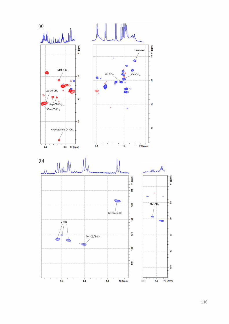
116

117
Figure 4.3. 400 MHz 1H-13C HSQC spectrum of an NP-C1 mouse liver aqueous extract: only
those resonances that were selected as discriminatory features and observable in a 1H-13C
HSQC spectrum (low concentrated metabolites are not visible in view of the low natural
abundance of 13C) are assigned in this Figure for purposes of clarity. Red cross-peaks indicate
either a -CH3 or -CH group, and blue ones represent -CH2- functions.
Figure 4.4. 400 MHz 1H-1H COSY spectrum, of an aqueous extract of an NP-C1 liver sample.
Typical spectra is shown (aromatic region expanded). Only the cross-peaks for the selected
metabolites are indicated in the spectrum. Abbreviations: Phe-C1/C2, Phenylalanine-C1/C2-

118
CH; Tyr-C3/C5, Tyrosine-C3/C5-CH; Tyr-C2/C6, Tyrosine-C2/C6-CH; Nic-C2, Nicotinate-C2-CH;
Lys/Orn, Lysine-C6-CH2/Ornithine-C5-CH2; Hypotau, Hypotaurine-C4-CH2SO2-; Met,
Methionine-C4-CH2; Val, Valine-CH¬3; Thr, Threonine-C3-CH; Nic/Nia-C4,
Nicotinate/Niacinamide-C4-H; Nia-C6, Niacinamide-C6-CH; Phe-C3/4/5, Phenylalanine-
C3/4/5-CH; Nia-C2, Niacinamide-C2-CH; Asp, Aspartate-C2-CH2a.
4.4.2.4. ROC curve analysis
In order to evaluate the ability of RFs to classify and predict using these variables, a
ROC analysis was carried out, using the corresponding option in MetaboAnalyst 3.0. Only
those variables detailed in the previous section were retained to perform the analysis
outlined above. Then, with only 11 variables (out of 143 initial variables) attributable to Phe,
Tyr, Val, Met/Hypotaurine, Niacinamide, Nicotinate, Lys/Orn, Thr, Asp, 3-
hydroxyphenylacetate and the unassigned bucket (0.77 - 0.80), RFs gave a maximum AUC
value of 0.939 (range = 0.823 - 1.000) (Figure 4.5).
In the ROC analysis observed in Figure 4.5, the number of variables is permuted to
generate different RF models containing different sets of variables from those previously
selected; furthermore, the number of features employed also changes. In this case, 2, 3, 5,
7, 10 and 11 variables were used for developing the models. For each model the respective
AUC value together with the range is stored and depicted in Figure 4.5.

119
Figure 4.5. (a) ROC curves analysis for the liver NP-C1 dataset and (b) blue bubbles indicate
metabolites with lower levels in NPC group and orange ones, those with higher levels. The
size of each bubble is correlated with the FC (fold change): different combination of variables
gave different AUC values ranging from 0.754 for 2 variables, up to 1 with 7, 10 and 11
variables, as indicated in the table inserted in the left plot. Abbreviations: TPR, True Positive
Rate; FPR, False Positive Rate; AUC, Area Under the Curve; U, unknown; 3-OH-PheAc, 3-
hydroxyphenylacetate.
ROC curve analysis revealed that the buckets attributable to 3-hydroxyphenylacetate
and tyrosine were the variables with higher frequency of selection for building up the
classification RFs models, additionally the models involving only 2 variables accomplished an
AUC range of 0.579 - 0.951 showing a good extent of success. These facts together with the
phenylalanine frequency of selection (0.96, ranked the 4th) indicate that the most affected
pathway in NP-C1 liver disease, and therefore the one with higher value as a discriminant
feature, is that involving aromatic amino acids.
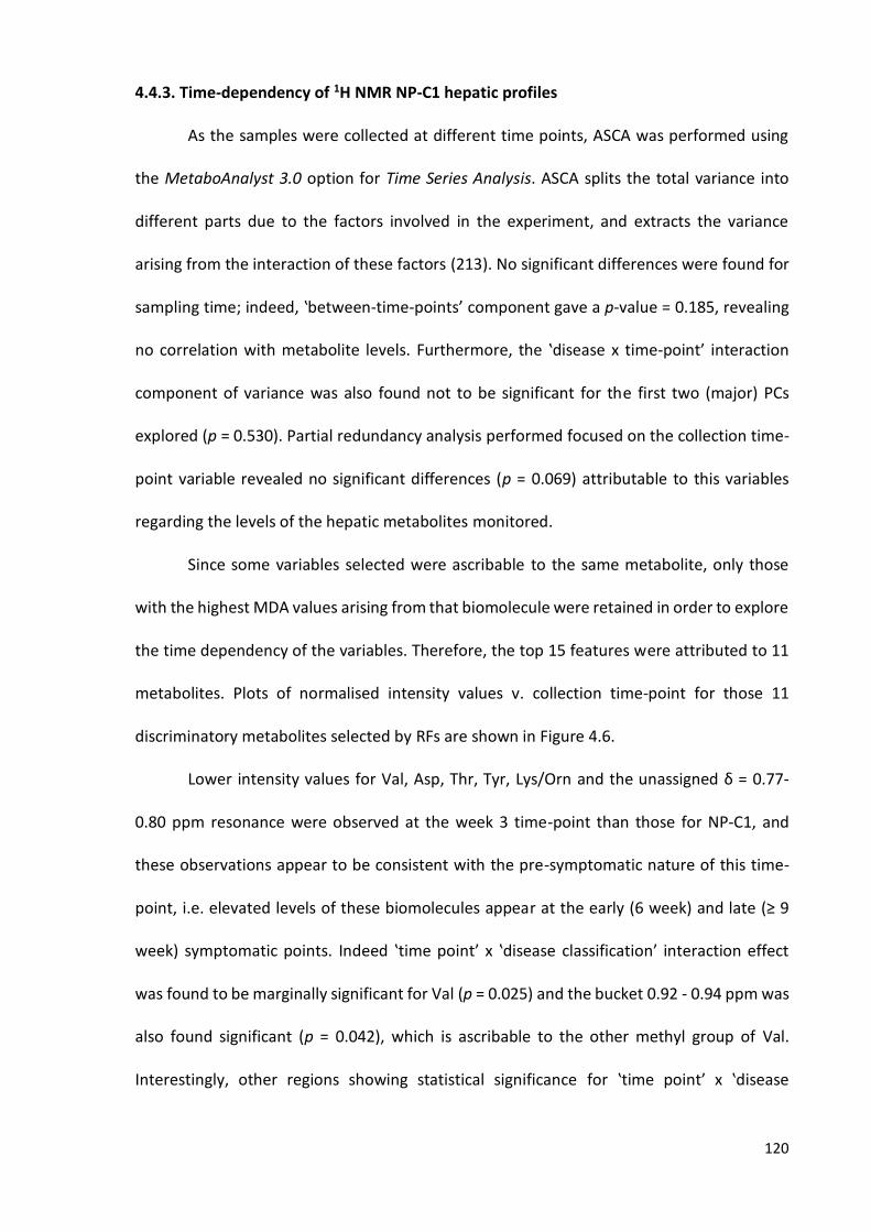
120
4.4.3. Time-dependency of 1H NMR NP-C1 hepatic profiles
As the samples were collected at different time points, ASCA was performed using
the MetaboAnalyst 3.0 option for Time Series Analysis. ASCA splits the total variance into
different parts due to the factors involved in the experiment, and extracts the variance
arising from the interaction of these factors (213). No significant differences were found for
sampling time; indeed, ‛between-time-points’ component gave a p-value = 0.185, revealing
no correlation with metabolite levels. Furthermore, the ‛disease x time-point’ interaction
component of variance was also found not to be significant for the first two (major) PCs
explored (p = 0.530). Partial redundancy analysis performed focused on the collection time-
point variable revealed no significant differences (p = 0.069) attributable to this variables
regarding the levels of the hepatic metabolites monitored.
Since some variables selected were ascribable to the same metabolite, only those
with the highest MDA values arising from that biomolecule were retained in order to explore
the time dependency of the variables. Therefore, the top 15 features were attributed to 11
metabolites. Plots of normalised intensity values v. collection time-point for those 11
discriminatory metabolites selected by RFs are shown in Figure 4.6.
Lower intensity values for Val, Asp, Thr, Tyr, Lys/Orn and the unassigned δ = 0.77-
0.80 ppm resonance were observed at the week 3 time-point than those for NP-C1, and
these observations appear to be consistent with the pre-symptomatic nature of this time-
point, i.e. elevated levels of these biomolecules appear at the early (6 week) and late (≥ 9
week) symptomatic points. Indeed ‛time point’ x ‛disease classification’ interaction effect
was found to be marginally significant for Val (p = 0.025) and the bucket 0.92 - 0.94 ppm was
also found significant (p = 0.042), which is ascribable to the other methyl group of Val.
Interestingly, other regions showing statistical significance for ‛time point’ x ‛disease

121
classification’ interaction effect were 1.70 - 1.74 and 1.74 - 1.79 ppm (p = 0.030 and 0.039)
which are ascribable to Lys-C5-CH2/Orn-C4-CH2 and 7.41 - 7.47 ppm (part of Phe multiplet,
p = 0.031). Nevertheless, those values may be considered marginally significant due to their
proximity to the threshold 0.05.
However, there appeared to be no time-dependence of the 3-hydroxyphenylacetate,
phenylalanine and nicotinate levels, although Val, Asp, Thr, Tyr and Phe NP-C1 hepatic levels
were higher than those of HET/WT group at all the post-symptomatic time-points, together
with lower ones for 3-hydroxyphenylacetate and nicotinate in this group. Although
niacinamide shows some descending tendency over time, such differences are clearly not
significant. Moreover, with the exception of 3-hydroxyphenylacetate, the liver content of all
metabolites appeared to be time-independent in the combined HET/WT group.
Performance of the above RF procedure, but excluding the pre-symptomatic week 3
samples, gave rise to a slight improvement compared to that achieved without removal,
specifically a mean OOB error of 0.13 ± 0.003, and prediction performance values for
sensitivity, specificity and accuracy of 0.86 ± 0.0014, 0.89 ± 0.0016 and 0.865 ± 0.00082
respectively. These results are consistent with the pre-symptomatic nature of samples
collected at the week 3 time-point in NP-C1 mice.
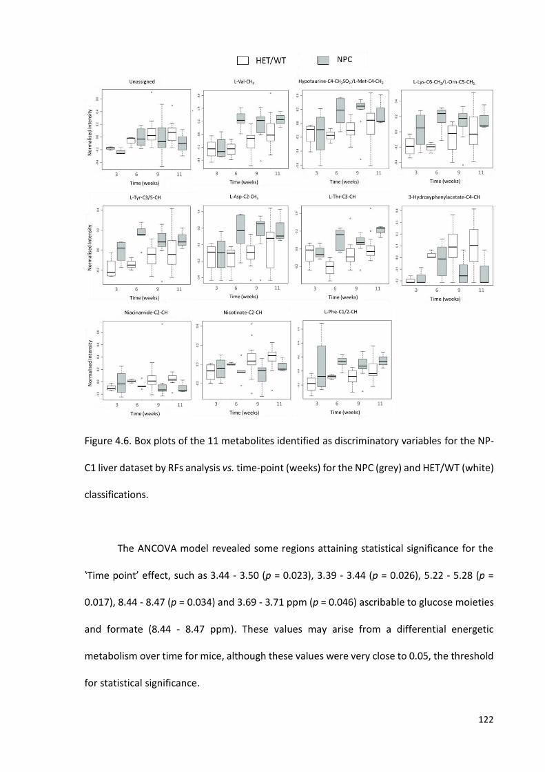
122
Figure 4.6. Box plots of the 11 metabolites identified as discriminatory variables for the NP-
C1 liver dataset by RFs analysis vs. time-point (weeks) for the NPC (grey) and HET/WT (white)
classifications.
The ANCOVA model revealed some regions attaining statistical significance for the
‛Time point’ effect, such as 3.44 - 3.50 (p = 0.023), 3.39 - 3.44 (p = 0.026), 5.22 - 5.28 (p =
0.017), 8.44 - 8.47 (p = 0.034) and 3.69 - 3.71 ppm (p = 0.046) ascribable to glucose moieties
and formate (8.44 - 8.47 ppm). These values may arise from a differential energetic
metabolism over time for mice, although these values were very close to 0.05, the threshold
for statistical significance.

123
4.4.4. Gender contribution to 1H NMR NP-C1 hepatic profiles
The same RF procedure described above was applied to the dataset, but in this case
the y response variable was gender. This analysis was performed to check that the variables
selected were not conditioned by gender differences and hence represent a true separation
between NP-C1 and healthy mice (WT/HET). The OOB obtained was 0.461 which reveals no
differences attributable to gender. Corresponding partial redundancy analysis-based
permutation testing analysis focused on the gender variable revealed that gender was not
significantly related to any of the discriminatory variables (p = 0.100). The only signals that
gave significant p-values for ‛gender’ contributions were 3.35 - 3.37 (p = 0.0065) , 5.17 - 5.20
(p = 0.0083), 3.44 - 3.50 (p = 0.024), 8.44 - 8.47 (p = 0.029), 5.88 - 5.93 (p = 0.035), 5.22 - 5.28
(p = 0.035) and 1.45 - 1.51 ppm (p = 0.040), ascribable to methanol, phosphoenolpyruvate-
CH2a (PEP), β-Glucose-C3/5-CH, formate-H, GTP-C1’-CH and α-glucose/glucose-6P-C1-CH
and alanine-CH3 respectively. Most of these metabolites are correlated with the glycolysis
pathway, since glucose subsequent transformed to glucose-6P yields PEP prior to the final
product, i.e. pyruvate, which can also arise from alanine in the alanine-pyruvate cycle. The
same variables shown significant p-values in the ANCOVA model for the factor ‛time point’ x
‛gender’, revealing no effect of the collection time point in those variables gender-
dependent. None of the variables presented a significant p-value for the interaction factor
‛disease’ x ‛gender’.
The variables listed in Table 4.2 failed to attain statistical significance for the ‛gender’
factor or any of the combinations with others, such as ‛disease’ and ‛time-point’, which
indicates that gender is not conditioning the classification of mice liver extracts according to
their disease class.

124
4.5. HEPATOCYTE REDOX STATUS BASED ON GSH:GSSG RATIO
Although not featuring as significant biomolecule variables in the RF and further MV
analysis models developed, we also explored differences between the mean hepatic
concentrations of glutathione (GSH) and its corresponding disulphide oxidation product
(GSSG), and in particular that of the [GSH]:[GSSG] concentration ratio between the NP-C1
and HET/WT classifications investigated. [GSH]:[GSSG] ratio is a valuable and reliable
indicator of the REDOX status of tissue, mainly in the liver, since this organ is the site of GSH
synthesis (214). GSH provides reducing equivalents to cells, and the GSH/GSSG couple is
recognised as a major thiol-disulfide cellular ‘redox buffering system’, since the combined
cellular concentrations of these biomolecules are much higher than those of the other two
major redox-active systems, i.e. NADP+/NAPH and thioredoxin (215). The levels of both
correlated metabolites can be utilised as indicator for the redox environment of the cell
(215). Glutathione is a tripeptide conformed for Glu-Cys-Gly, in which Cys is the key
component, since its reactive thiol group is the one involved in the formation of a disulphide
linkage with an additional GSH molecule to yield GSSG (Equations 21 and 22).
GSH + •OH GS• + H2O (21)
GS• + GS• GSSG (22)
The buckets selected to explore the levels of GSH and GSSG were 4.55 - 4.61 ppm and
3.31 - 3.35 ppm (Figure 4.7), attributable to GSH-Cys-CH and GSSG-Cys-CH2a respectively,
according to the chemical shift values provided in (216) and (217) respectively.

125
Figure 4.7. Typical spectra from an aqueous liver tissue extract from 3.15 ppm to 4.62 ppm
showing the resonance signals employed for the [GSH]:[GSSG] computation.
Primarily, it was found that hepatic GSH levels were significantly reduced in NP-C1
patients (p = 0.036), although no such differences were noted for GSSG (ANCOVA model
depicted in Equation 20) for the ‛between-disease classifications’ factor However, there was
a much more highly significant decrease in the mean [GSH]:[GSSG] ratio of the NP-C1 group
when compared to that of the HET/WT control one (p = 8.65 x 10⁻⁴).
Figure 4.8. (a) Box plot for hepatic mice GSH:GSSG ratio [4.55 - 4.61]:[3.31 - 3.35] and (b) for
hepatic mice GSH levels for both disease classification groups: Both GSH and GSH:GSSG ratio
were analysed using the ANCOVA model depicted in Equation 20, showing a significant
difference (p < 0.05, *; p < 0.01, **; p < 0.001, ***).

126
CHAPTER 5
CLASSIFICATION AND VARIABLE SELECTION BY
RANDOM FORESTS AND CORRELATED
COMPONENT REGRESSION IN A METABOLOMICS
CONTEXT
5.1. RANDOM FORESTS RANKING FOR VARIABLE SELCTION vs. RANDOM FORESTS-
RECURSIVE FEATURE ELIMINATION
NP-C1 Disease Urinary dataset: In order to identify the variables which were more
important for the discrimination of samples according to their disease classification, MDA
values for each variable were saved at each iteration and finally averaged to obtain final
rankings. Additionally, it was possible to track the ranking and MDA value of any variable
along all those 100 repetitions (Figure 5.1) in order to explore their variability. At each
iteration the whole sample set was partitioned as 2/3 for training and 1/3 for test sets, and
hence 100 different sub-sets of training and test sets were employed.
An alternative methodology for variable selection is Recursive Feature Elimination
(RFE), an approach which is linked to the RFs technique (RFs-RFE). RFs-RFE is a strategy

127
proposed by Diaz-Uriarte (218) in which 20% of variables with lowest ranking are removed
after RFs performance, and then the classification is performed again without those
variables. The ability of this process is assessed by the OOB error value, i.e. variables with
lowest contribution for classification will be removed until this value (OOB error) increases
or becomes unstable.
Figure 5.1. (a) MDA values for top-5 variables ranked by RFs over 100 iterations in which the
black line represents the MDA mean value (0.88) of the 15th variable selected by RFs for the
urinary NP-C1 dataset, and this acts as a threshold for variable selection. (b) Recursive
Feature Elimination (RFE) for the urinary NP-C1 dataset showing changes in the OOB error
value as a function of the number of variables employed by the RFs analysis.

128
Creatinine-N-CH3 (4.05 - 4.10 ppm), 3-aminoisobutyrate-CH3 (1.17 - 1.22 ppm),
unknown-1 (0.72 - 0.76 ppm), and both trigonelline signals [-C4/6-CH (8.80 - 8.86 ppm) and
-C2-CH (9.11 - 9.16 ppm)] were selected below the mean MDA value obtained for the 15th
top variable (2-Hydroxyisobutyrate-CH3’s, 1.36 - 1.41 ppm) 7%, 10%, 13%, 19% and 20%
respectively. The 16th ranked variable was the 1.58 - 1.63 ppm bucket assignable to 5-
aminovalerate-C3/4-CH2, with an MDA value of 0.79. This metabolite was selected by the
CCR and GAs techniques as the 12th and 10th most important variable respectively.
In Figure 5.1 (b) the OOB error value decreases until the number of variables is 23,
then it becomes stable and then starts to fluctuate as the number of variables further
decreases. However, even with only 3 variables, the OOB error value obtained was 0.149, a
value below 0.220 which is the starting OOB value with 219 variables. These last 3 variables
were the 0.72 - 0.75 ppm, 1.17 - 1.22 ppm and 4.05 - 4.10 ppm buckets, the latter two
assigned to 3-AIB and Cn respectively.
Mice hepatic dataset: The variability of the variables ranking, and consequently, the
features selected after the full cross-validated process was also explored for the NP-C1 liver
dataset. The combined top-5 ranked variables’ MDA value was explored over each of those
100 repetitions, and is depicted in Figure 5.2. The performance of RFs-RFE was also explored
to compare with the RFs variable selection procedure.
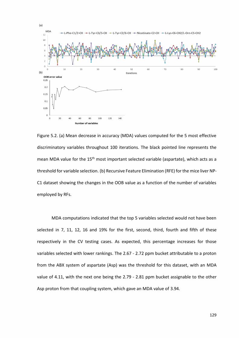
129
Figure 5.2. (a) Mean decrease in accuracy (MDA) values computed for the 5 most effective
discriminatory variables throughout 100 iterations. The black pointed line represents the
mean MDA value for the 15th most important selected variable (aspartate), which acts as a
threshold for variable selection. (b) Recursive Feature Elimination (RFE) for the mice liver NP-
C1 dataset showing the changes in the OOB value as a function of the number of variables
employed by RFs.
MDA computations indicated that the top 5 variables selected would not have been
selected in 7, 11, 12, 16 and 19% for the first, second, third, fourth and fifth of these
respectively in the CV testing cases. As expected, this percentage increases for those
variables selected with lower rankings. The 2.67 - 2.72 ppm bucket attributable to a proton
from the ABX system of aspartate (Asp) was the threshold for this dataset, with an MDA
value of 4.11, with the next one being the 2.79 - 2.81 ppm bucket assignable to the other
Asp proton from that coupling system, which gave an MDA value of 3.94.

130
In this study, the RFs strategy was applied for the classification of human urine and
plasma, together with mice liver samples according to their disease status. In this case, RFs
was employed with the major aim of determining the variables that can group samples based
on their disease class; in this manner, we can enhance our knowledge of disturbances in
metabolic pathways arising from the NP-C1 disease process, and moreover propose some of
these metabolites as biomarkers.
A wide range of different MVA techniques are available for variable selection (219),
but RFs attain effective results when dealing with outliers, it does not overfit and provides
excellent results even if some variables are noise (220). Several MVA strategies have been
successfully utilised for the analysis of datasets in which the number of possible predictor
variables (P) exceeds the number of samples (n) available, i.e. P > n situations; one of these
techniques is the RFs approach, which has been successfully applied throughout a range of
metabolomics studies (221, 222).
Our RFs model was primarily tuned in order to improve its performance, and this
approach has been previously investigated by Diaz-Uriarte et al. (218), in which the
investigators demonstrated that both the number of variables included in the generation of
each individual tree, and the maximum number of trees included in the final RFs model can
be tuned separately since they are independent parameters. Moreover, the computational
time required proportionally increases with the number of trees, and selecting a very large
number does not necessarily provide an improved performance, as reported in (218) and
explored in this investigation. The number of variables selected for tree partitioning has
been shown to be the most critical parameter to tune; nevertheless, the default value was
found to be an effective choice for the liver and plasma NP-C1 datasets, in which it was set
at a value of (143)1/2 ≈ 12 for liver, and 7 for plasma, given the presence of a total of 39

131
variables in the latter dataset (for this model, 6 or 7 variables for tree partitioning would
have matched the √𝑛 rule). Nevertheless, when RFs strategy was applied to the urinary NP-
C1 dataset, the optimal value for tree partitioning was 8, a very low value considering the
total number of variables in the original dataset (199 variables).
The variable selection process has been performed based on the MDA values, since
this has been suggested to be the most reliable metric (79, 223), and therefore it is more
robust than the other available metric, the Gini index (224). In view of the random sub-
sampling procedure conducted by RFs for classification purposes, the variables with
selectively higher MDA values can, of course, vary when this classification technique is
repetitively applied to MV analysis of the same dataset; moreover, in order to explore as
many combinations of samples in the training and test sets as possible, an iterative process
was implemented here, although the OOB error term computation already involves a cross-
validation (CV) procedure (225).
An assessment of the performance of this iterative cross-validated process was also
conducted in order to test the reliabilities of the selected metabolite variables, and this
revealed that with the employment of the MDA value of the 15th-ranked variable as a
threshold, the top 1-, 2-, 3-, 4- and 5-ranked variables selected would not have been selected
in 7, 11, 12, 16 and 19% respectively of the CV testing cases (Figure 5.2) for the liver dataset,
and 7, 10, 13, 19 and 20% respectively for the NP-C1 urinary one (Figure 5.1), which shows
how the variables selected change with different test and training sub-sample sets.
Therefore, studies in which CV with random sub-sampling is only performed once or a few
times can experience this limiting effect, since the results can be biased by the sub-sample
selected. However, the robustness of this ensemble technique was confirmed by the
computation of SEM values for the MDAs, which were very small.
132
Additionally, a further major methodology available for variable selection, the so-
called Random Feature Elimination, serves as another iterative process which was first
proposed by Diaz-Uriarte (218). When combined with RFs, the variable importance is
primarily computed, and this process then repeated with removal of the 20% of less
important variables until the OOB decreases to a stable value. This strategy was also
explored herein employing our urine and hepatic datasets, which revealed how the OOB
value initially decreases with the reduction of the number of variables (20% at each
repetition), an observation predominantly ascribable to the removal of noisy variables that
generate unsuccessful trees, and that are further averaged when computing the OOB.
Additionally, this procedure has been investigated in detail in (226).
In the datasets investigated, the OOB error value reached a minimum and then
became unstable, i.e. a high variability of OOB error values following the removal of certain
variables; however, even using only 3 variables, the OOB error value was lower than the
initial one containing the complete set of features, indicating an improved classification
performance. The main issue arising from this RFE approach is that the final goal of this
strategy is to reduce the number of variables to the minimum, whilst maintaining reasonably
good classification performance; nevertheless, in a metabolomics context, where the
selected features might be related to disorders caused by the disease and not by the disease
itself, reductions in the number of variables can be detrimental, since information about
affected pathways may be lost, and the reduced number of variables may represent common
metabolites that usually are non-disease-specific, and therefore their value as biomarkers is
severely limited.

133
5.2. CORRELATED COMPONENT REGRESSION: A NEW TOOL FOR METABOLOMICS
ANALYSIS
5.2.1. CCR-LDA performance
Correlated Component Regression-Linear Discriminant Analysis (CCR-LDA) was
applied to the urinary and liver NP-C1 datasets to evaluate its ability to classify those samples
with regard to their disease status, and also to compare its performance against other well-
established MVA techniques employed in metabolomics investigations. The results arising
from both these classification problems are depicted in the table below.
Table 5.1. MVA performance of all the technique employed for the urinary and liver NP-C1
datasets: the top part of the Table is a copy of Table 3.2. The bottom part includes the
analysis outlined in section 4.4.2.2 plus the results of the CCR-LDA applied to the hepatic
dataset. The OOB error value is also indicated for the RFs approach (the standard error of
the mean for each of the parameters computed is shown in brackets).
CCR-LDA only out-performs the other techniques in term of specificity, although it
presents higher SEM values for all the parameters computed. The main difference, however,
is the low value obtained for sensitivity. This dataset is somewhat complicated, since the 2
Dataset MVA Technique OOB (SEM) Accuracy (SEM) Sensitivity (SEM) Specificity (SEM)
UR
INE
RFs 0.224 (0.00012) 0.835 (0.001) 0.695 (0.001) 0.831 (0.003)
GA-MLHD/SVM - 0.827 (0.002) 0.752 (0.002) 0.903 (0.001)
CCR-LDA - 0.810 (0.013) 0.583 (0.032) 0.926 (0.012)
LIV
ER RFs 0.190 (0.0004) 0.810 (0.001) 0.799 (0.001) 0.843 (0.003)
CCR-LDA - 0.824 (0.014) 0.719 (0.029) 0.887 (0.016)

134
classes are not balanced, and the control group is almost 4 times larger than the disease one.
Therefore, the CCR strategy could be more sensitive to that issue.
The main feature that CCR-LDA has when compared to alternative parametric MVA
techniques is the correlation of the components, so that these are not selected with the
restriction of having to be orthogonal to each other, but with the aim of improving the
performance of the model, increasing the ability of the component previously selected for
classification (in the case of the combination with LDA, it can be employed for regression
purposes in addition). Those components contributing to the overall performance via
enhancements of the predictive ability of the pre-built model are known as proxy
components, and those variables with higher loading on those components and lower on the
prior ones are denominated proxy (suppressor) variables.
5.2.2. CCR-LDA dependency of the number of components and variables employed
In order to explore the ability of the CCR-LDA technique to classify samples
independently of the number of variables and/or components employed to construct the
model, the number of variables was limited to 5, 10, 15 and 20, and the number of
components to 1, 2 and 3 for both urinary and hepatic mouse datasets; selecting each of
these combinations 5 times yields a final set of 60 different models. Specificity, sensitivity,
accuracy and AUC values were computed for each of these models. For each of those 12
possible combinations of maximum number of components x maximum number of variables,
the classification performance parameters were averaged.

135
Figure 5.3. CCR-LDA results for the NP-C1 urinary dataset. (a) Scatter plot of the number of
variables vs. the parameters employed for the 60 models generated utilising from 1 to 20
variables. (b) Mean values for specificity (Spec), sensitivity (Sen), accuracy (Acc) and area
under the curve (AUC), along with their SEM values for the models generated with 1, 2 and
3 components. (c) Individual density plots for specificity, sensitivity, accuracy and AUC as a
function of the total number of variables employed by the CCR-LDA strategy.
No significant correlations (linear, logarithmic or quadratic) were found between the
number of variables employed for the model and their classification performance (Figure
5.3). Indeed, analysis of the classification performance as a function of the number of
components did not show any tendency for sensitivity and accuracy to increase; however, it
should be considered that specificity decreases as the number of components increase, and

136
also the opposite effect is observed for AUC values in Figure 5.3(c). In the density plots it can
be observed that neither sensitivity nor accuracy show a tendency (decreasing or increasing
values as the number of components increases); however, sensitivity values appear to
increase with the number of variables, and for the AUC, these values increase with only a
few variables, and then they remain at a high level when more variables are introduced into
the model.
Figure 5.4. CCR-LDA results for the NP-C1 mice hepatic dataset. (a) Scatter plot of the number
of variables vs. the parameters employed for the 60 models generated utilising from 1 to 20
variables. (b) Mean values for specificity (Spec), sensitivity (Sen), accuracy (Acc) and area
under the curve (AUC), along with their SEM values for the models generated with a

137
maximum of 1, 2 and 3 components. (c) Individual density plots for specificity, sensitivity,
accuracy and AUC as a function of the number of variables employed by CCR-LDA.
Values for specificity, sensitivity, accuracy and AUC in the NP-C1 mice liver CCR
analysis of the 1H NMR spectral buckets reveals a clear dependency of the number of
components, these parameters increasing with the number of components involved (Figure
5.4). Nevertheless, no tendency or dependency is observed regarding the number of
variables employed, although lower values for these parameters are obtained when the
number of variables is less than 10, except for that of sensitivity which reaches its minimum
value when the number of features employed are close to 15.
The variable selection process in CCR is analogous to the RFE one described in section
5.1, since the ‛step-down’ procedure incorporated in the CCR algorithm starts with the whole
set of variables and they are then sequentially removed until the CV process performance
decays. With regard to classification problems, the minimum number of variables is always
desired for a model, so that a low number of variables can be set as an initial parameter for
CCR, and then researchers may check to determine if a successful classification rate is
accomplished. In this case, a limitation to only 5 variables out of 219 and 143 for the urinary
and hepatic datasets, respectively, were set, and results arising from CCR-LDA model gave
very promising results. Nevertheless, the lowest values for sensitivity, accuracy and AUC
were obtained using 5 variables [Figure 5.3 (c)] for the urinary dataset. The same results
were observed in the hepatic dataset [Figure 5.4 (c)]. However, there is not a very high
density of points in Figures 5.2 (c) and 5.3 (c), an observation that may indicate that limitation
of variables affects the results for these datasets, as expected.

138
CHAPTER 6
INTEGRATIVE METABOLOMICS: URINE, PLASMA
AND LIVER 1H NMR METABOLOMICS ANALYSIS
TO ASSESS THE METABOLISM OF NP-C1
PATIENTS
6.1. NICOTINATE/NIACINAMIDE PATHWAY
Elevated levels of quinolinate (p = 3.83 x 10⁻⁵, FC = 30.32) were found in urine
specimens collected from NP-C1 patients, and the 1H NMR analysis of liver samples collected
from NP-C1 mice model also showed lower levels of nicotinate (p = 1.30 x 10⁻³, FC = -1.49)
and niacinamide (p = 0.26, FC = -1.01) than in healthy controls. These findings suggest an
imbalance in the nicotinate/niacinamide pathway that may, in turn, lead to a depletion in
NAD/NADP levels.
Dietary nicotinamide is absorbed in the intestines, and it is then converted in the
intestinal lumen by bacterial nicotinamidase to nicotinate. Both nicotinamide and nicotinate
are major precursors of NAD synthesis in humans (salvage pathway), even though they are
required to be incorporated through the diet. Moreover, human cells have the ability to
139
synthesise NAD from tryptophan (Trp) (Figure 6.1). Hara and co-workers have suggested
that NAD biosynthesis is tissue-specific based on the expression pattern of the enzymes
involved in its metabolism (227). Hence, it occurs predominantly from nicotinate in the small
intestine and from nicotinamide in skeletal muscle, whereas in the liver and kidney, both
metabolites, along with Trp, contribute to the synthesis of NAD (227). Moreover, NADP is
synthetised through the phosphorylation of NAD, and particularly noteworthy is the
diminished mean hepatic concentration of GSH present in the NP-C1 mouse classification (p
= 0.036), which may reflect a disease-mediated imbalance in hepatocyte [NADP+]:[NADPH+]
concentration ratios, since GSH is required for the conversion of NADP to NADPH (228).
The first step in NAD synthesis from nicotinamide is the generation of its
mononucleotide, a reaction mediated by the enzyme nicotinamide
phosphoribosyltransferase (Nampt). A recent investigation has reported an upregulation of
Nampt mRNA, and increased levels of NAD in the liver of mice fed with a high-fat diet (229),
and also in non-alcoholic fatty liver disease (NAFLD) (230). Additionally, Nampt mRNA
expression levels were also found to be higher in fibrotic human livers (231), fibrosis being a
major feature of the development of NP-C1 mice liver pathophysiology (122). Therefore, the
hepatic stress experienced by the NP-C1 mice could lead to an increase in NAD production
in order to load enzymatic reactions that require this cofactor, such as β-oxidation and
tricarboxylic acid metabolism which are enhanced in other hepatic disorders such as NAFLD
(232). Indeed, in NAFLD liver tissue, there is an imbalance in bile acid duct transporters (233),
a complication also observed in NP-C1 mice liver as discussed below. This enhanced
requirement of NAD may be responsible for the low nicotinate/nicotinamide levels observed
in NP-C1 mice liver extracts, since they appear to be overutilised to generate NAD.

140
Moreover, the increased levels of quinolinate (QUIN) found in urine collected from
NP-C1 patients, together with the lower levels of both nicotinate and niacinamide in NP-C1
mice hepatic tissue, could indicate an imbalance between de novo and salvage pathways,
i.e., an overloading of the latter in NP-C1 liver. The synthesis of NAD from Trp via QUIN
mainly occurs in the liver (234); therefore, a defect in the QUIN to nicotinate mononucleotide
stage may lead to an increased activity of the salvage pathways enzymes, hence reducing
the levels of nicotinate/niacinamide and therefore the accumulation of QUIN that is then
released from hepatocytes. Healthy individuals, with sufficient dietary levels of
nicotinamide, present relatively low levels of QUIN production in the liver, and consequently
its levels, together with those of further kynurenine pathway metabolites in other tissues
and the systemic circulation are relatively low (235).
Figure 6.1. NAD metabolism: schematic representation of NAD synthesis highlighting those
metabolites selected as discriminatory variables, and indicating the tissue/biofluid where
they were found, and their levels in NP-C1 samples expressed relative to those from healthy
controls. Urinary metabolites selected by the different strategies applied are indicated by
coloured boxes (red = RFs; green = GAs-SVMs/MLHD; blue = CCR-LDA). Metabolites
141
highlighted in orange refer to those selected in mice liver samples analysis. Arrows illustrate
higher (↑) or lower (↓) levels in the NPC group.
Quinolinate (QUIN) is generated and released by infiltrating macrophages and
activated microglia in the brain (236). It is produced through the kynureine pathway, which
is the route involved in the degradation of Trp and the production of NAD (Figure 6.1). QUIN
acts as an agonist of the N-methyl-D-aspartate (NMDA) receptors, mainly in the forebrain,
and as such is considered to be an endogenous brain excitotoxin. This gives rise to a wide
range of deleterious processes within the brain through its triggering of ionic imbalances in
neurons via a Ca2+ influx which activates a NMDA-receptor (237). Moreover, activation of
neuronal nitric oxide synthase and nitric oxide activity (238), together with and cytoskeleton
destabilization (239), may also lead to cell death. Since QUIN does not have a specific
transporter to cross the BBB (240), the increased levels of this metabolite found in NP-C1
urine samples presumably arise from other tissues, since macrophages have a 20-fold higher
ability to generate QUIN than that of microglial cells (241). Additionally, the liver also has the
ability to generate QUIN (242).
The increase of QUIN levels in biofluids has been previously reported, with elevated
concentrations in blood serum and cerebrospinal fluid (CSF) being correlated to early renal
insufficiency (243). Indeed, a method to quantify QUIN in urine using LC-MS/MS (244) has
recently been proposed for the diagnosis of renal cell carcinoma, i.e., urinary QUIN may serve
as a biomarker (245). Furthermore, its levels have been also observed to be elevated in sepsis
processes (246), such levels being linked to an immune system response mainly dominated
by macrophage activation. Elevated levels of QUIN in urine could arise from a macrophage
infiltration, which has been observed in several tissues such as lungs (247) and liver (120) in
142
both human and mice afflicted with NP-C1 disease. Indeed, more recently increased serum
levels of QUIN have also been observed in hepatic dysfunction (248).
6.2. BLOOD PLASMA LIPOPROTEIN PROFILES
A major cellular process in NP-C1 disease is the disruption of cholesterol transport
from the lysosome. This cholesterol arises from LDL particles that are transported via the
bloodstream. Given these pathological features, it may be expected that significant changes
occur in lipoprotein homeostasis in NP-C1 patients. Indeed, recent studies have revealed
that the plasma lipoprotein profile of NP-C1 patients is characterised by low HDL, LDL and
total cholesterol levels, and higher TG levels (249). It has also been observed that a reduction
in HDL-cholesterol levels is correlated with the impairment of cholesterol trafficking within
the cell (249, 250).
Intriguingly, in this work, the LDL-(CH2)n spectral region presented a similar pattern
following the NPC ≈ MGS ≈ HET >> WT classifications. The 1H NMR plasma profiles of NP-C1
patients revealed higher levels for both VLDL signals than the WT one (Figure 4.4). Since the
-(CH2)n, -CH2CH2CO, and N-acetyl glycoprotein/CH2-CH2-CH= mobile lipid regions of the NMR
spectra acquired have been previously shown to be strongly correlated with plasma
triglyceride levels in both humans and mice (251, 252), this is consistent with elevated
lipoprotein-associated TG levels in the NP-C1, MGS and HET groups over those of the WT
one observed in this study, even though the WT samples were collected under non-fasting
conditions.
Interestingly, nicotinate is an inhibitor of hepatocyte microsomal diacylglycerol
acyltransferase 2 (DGAT2), an enzyme involved in the synthesis of TGs from DGs (253). When
this metabolite inhibits hepatic DGAT2, TG synthesis is decreased, and concomitantly, its
143
availability for VLDL assembly; as a consequence, apoB degradation is increased and the
secretion of VLDL/LDL particles is diminished (254). Therefore, in cases of diminished
nicotinate levels, VLDL particles should be increased in plasma, as observed in this work.
Intriguingly, a study performed by Beltroy et al. (122) showed that TGs levels in the hepatic
tissue of NP-C1 mice are lower than those of corresponding healthy controls. In contrast, in
another study performed by Garver and co-workers, lipid levels in both NP-C1 and WT mice
were found to be not significatively different, with surprisingly elevated levels of TGs in a
HET mice group (121). In this work, the HET group involved also exhibited enhanced levels
for the VLDL-CH3 and -(CH2)n spectral regions when expressed relative to those of the WT
group, indicating that heterozygotes may also present increased plasma TGs levels, and
suggesting that this increase is not directly linked to disease pathology [which is consistent
with the lack of correlation between TGs and age of death in previous reports (249)] or that
they present an intermediate phenotype for VLDL metabolism.
The HDL-(CH2)n- variable exhibits a pattern in the classification order HET > MGS >
NPC >> WT, and this was selected by RFs analysis as the 2nd most important variable when
determining differences between the NPC and HET groups. The higher levels of this
lipoprotein contrast with those found in other cholesterol storage disorders (besides NP-C1),
such as Tangier disease (255) and cholesterol ester storage disease (256). HDL levels in
heterozygotes have been previously reported as not generally affected (250), an observation
contrary to the results reported here. MGS-treated patients show a slight increase in their
HDL levels when compared to those from the NPC group, which is in accordance with
investigations using MGS with Gaucher patients (257); in contrast, this improvement in HDL
metabolism was not observed when treating Tangier disease patients with this agent (258).
This effect on HDL levels is potentially attributable to the imbalance in ABCA1 protein

144
activation that occurs in NP-C1 cells, since ABCA1 is the central protein involved in HDL
metabolism (250).
6.3. BILE ACID METABOLISM
Increased levels of bile acids (BAs) were observed in the urinary profiles of NP-C1
patients (p = 9.39 x 10⁻⁵, FC = 8.54); indeed, the variable 0.66-0.69 ppm was selected within
the top 8 features for classification by all the MVA techniques employed for the urinary
dataset analysis employed. This bucket contains resonances ascribable to the C18-CH3 group
of glycochenodeoxycholate, chenodeoxycholate, taurochenodeoxycholate,
taurodeoxycholate and tauroursodeoxycholate, the latter being a BA encountered in
humans at very low levels (259); indeed, about 4% of total bile is ascribable to this BA (260).
The primary bile acids are cholate and chenodeoxycholate, since they are synthetized in the
liver by the action of human enzymes; subsequently, further biotransformations carried out
by human microbiota lead to the formation of lithocholate, deoxycholate and
ursodeoxycholate.
As previously noted, urinary concentrations of BAs are increased in pathological
situations where the hepatobilary system is compromised. These increased urinary levels of
BAs could arise from the cholestasis and liver disease that are features of NP-C1 disease (91).
Erickson et al. have shown how mRNA levels for the BA transporters Mrp1, 2, 3, 5 (multi-
drug resistance proteins) and Ntcp (Na+-taurocholic co-transporting polypeptide) were
elevated in NP-C1 mice, an observation suggesting that this transcriptional upregulation is a
compensatory mechanism in hepatic stress situations, and is required to potentiate the
excretion of any potentially toxic agents (125). The increased expression of these sinusoidal
excretion transporters may cause an enhancement in BA excretion from the liver into the
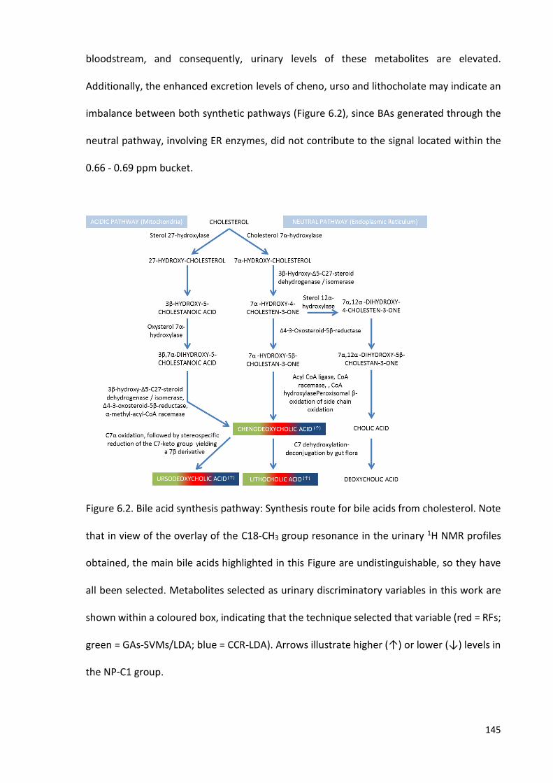
145
bloodstream, and consequently, urinary levels of these metabolites are elevated.
Additionally, the enhanced excretion levels of cheno, urso and lithocholate may indicate an
imbalance between both synthetic pathways (Figure 6.2), since BAs generated through the
neutral pathway, involving ER enzymes, did not contribute to the signal located within the
0.66 - 0.69 ppm bucket.
Figure 6.2. Bile acid synthesis pathway: Synthesis route for bile acids from cholesterol. Note
that in view of the overlay of the C18-CH3 group resonance in the urinary 1H NMR profiles
obtained, the main bile acids highlighted in this Figure are undistinguishable, so they have
all been selected. Metabolites selected as urinary discriminatory variables in this work are
shown within a coloured box, indicating that the technique selected that variable (red = RFs;
green = GAs-SVMs/LDA; blue = CCR-LDA). Arrows illustrate higher (↑) or lower (↓) levels in
the NP-C1 group.

146
Increased BA levels observed in the urinary profiles of NP-C1 patients may also (or
alternatively) arise from the unusual bile acid 3β,7β-dihydroxy-5-cholen-24-oate (which is
doubly-conjugated with sulphate at C-3, and N-acetylglucosamine at C-7), and/or its glycine
and taurine C-24 position adducts (261), agents which may serve as valuable urinary
biomarkers for this disease and perhaps reflect associated liver trauma in these patients
(262). Moreover, in the work published by Alvelius et al. (263), higher urinary levels of C24
3b-sulfooxy-7b-N-acetylglucosaminyl-5-cholen-24-oic bile acid (SNAG-D5-CA), together with
its glycine and taurine-conjugates, were found to be elevated for NP-C1 patients when
compared with healthy controls, and a LC-MS/MS methodology has been recently reported
for the measurement of this BA in urine (262). Based on the chemical structures of both BAs
in which the position 12 is not hydroxylated, they may contribute towards the signal located
within the 0.66 - 0.69 ppm bucket.
6.4. MUSCLE BIOMASS WASTING
Common clinical features of NP-C1 disease are weight loss and loss of muscle biomass
(264, 265). Consequently, the release of muscle breakdown products, such as branched-
chain amino acids (BCAAs) and correlated metabolites into the bloodstream, which can then
be filtered out into urine may serve as an indicator of this process.
BCAAs can be neither stored nor biosynthesised in the human body; therefore, their
levels are conditioned by the diet, the proteolysis of endogenous proteins and the
degradation that takes place in mitochondria. BCAA catabolism occurs in skeletal muscle,
liver, kidney, heart, brain and adipose tissue. Although they cannot be synthetized de novo,
their degradation products can be incorporated into other biomolecules such as lipids, since
Val, Leu and Ile ultimately yield propionyl-CoA and/or acetyl-CoA from their catabolism.

147
Muscle protein contains a higher proportion of BCAAs than that of proteins in other
tissues, and muscle is the predominant site of their degradation. Indeed, a urinary 1H NMR-
based metabolomics study on muscle wasting revealed that the concentrations of BCAAs,
together with their oxidation products, are increased in urine collected from patients
suffering from this debilitating condition (266).
In this study, the Val-CH3’s/Ile-CH3a bucket (0.98 - 1.03 ppm) was selected as a
discriminant feature by the CCR-LDA approach in view of its higher level in the NP-C1 1H NMR
urinary profiles (p = 1.65 x 10⁻², FC = 5.06), and Ile was also highlighted in plasma, having
considerably higher levels in NP-C1 patients (p = 5.51 x 10⁻¹¹, FC = 1.47), along with those of
the HET and MGS groups. Additionally, 3-AIB (p = 8.58 x 10⁻⁹, FC = 2.81) was selected by the
RFs and CCR techniques with very high rankings (2nd for RFs, 1st for CCR-LDA), this being a
common metabolite for the valine and thymine degradation pathways. Therefore, this may
serve as a hallmark of muscle wasting, since increased BCAA levels have been previously
reported to be correlated to rises in muscle protein deterioration (267). Another two BCAA
metabolites were selected as discriminatory features in our urinary dataset, specifically 2-
hydroxy-3-methylbutyrate (p = 8.47 x 10⁻³, FC = -10.22) and 3-hydroxyisobutyrate (p = 7.23 x
10-2, FC = 1.19). 2-hydroxy-3-methylbutyrate is generated through the reduction of 2-
oxoisovalerate, a catabolite of Val, and 3-hydroxyisobutyrate is a further metabolite in the
same pathway (Figure 6.3). The lower levels of this metabolite, together with those higher
values for 3-AIB urinary concentrations, may indicate an increased activity of the enzymatic
system that yields isobutyryl-CoA from 2-oxoisovalerate (Figure 6.3). Nevertheless, the
spectral region to which 3-hydroxyisobutyrate was assigned may indeed contain other
resonances arising from the α-CH group of amino acids, which may represent a confounding
factor.

148
Figure 6.3. BCAA degradation metabolic pathway: this route, as part of the BCAA catabolism
process, was indicated as one of the major pathways affected in the disease (leucine
catabolism is not included). The thymine catabolism route is also incorporated into this
diagram since its final product is common to that of the valine degradation pathway. Urinary
metabolites selected as discriminatory variables are visible within a coloured box, which also
indicates the technique that selected that variable (red = RFs; green = GA-SVM/LDA; blue =
CCR). Plasma discriminatory features for the NP-C1 vs. WT comparison are indicated by a red
coloured circle. Arrows illustrate higher (↑) or lower (↓) levels in the NPC group.
Intriguingly, loading evaluations with both thymine and L-Val have revealed that
urinary 3-AIB predominantly arises from thymine catabolism, with ≤ 10% generated from L-
Val degradation (268, 269). High 3-AIB urinary levels have also been observed in cases of

149
methylmalonic semialdehyde dehydrogenase deficiency (268), an enzyme involved in the
catabolic breakdown of both Val and thymine. Metabolism of valine produces the
intermediate (S)-3-hydroxyisobutyric acid, a metabolite that may be elevated in urine from
NP-C1 patients (p = 7.23 x 10⁻², FC = 1.19), although its 1H NMR signal at 3.67 - 3.71 ppm
overlaps with that from the α-CH group of amino acids, so this assignment remains tentative.
3-Hydroxyisobtyrate is then oxidized to (S)-methylmalonate semialdehyde by 3-
hydroxyisobutyrate dehydrogenase. Thymine metabolism generates 3-AIB, which is then
deaminated to (R)-methylmalonate semialdehyde. These two enantiomers are substrates
for methylmalonate semialdehyde dehydrogenase, which catalyses their oxidative
decarboxylation to propionyl-CoA (Figure 6.3).
Glutamine (Gln) was also selected as a urinary discriminatory feature, but only by the
RFs approach (and ranked as the 6th most important), having higher levels for NP-C1 patients
(p = 2.61 x 10⁻², FC = 1.49). The plasma pool of Gln has been proposed to arise from its release
from skeletal muscle (270, 271), which may be another indicator of muscle wastage. Indeed,
increased levels of the Gln bucket were also found in our plasma dataset (p = 7.95 x 10⁻⁷; FC
= 1.23) for the NP-C1 group when expressed relative to those of the WT classification.
Moreover, increased urinary levels of Cr (p = 1.52 x 10⁻⁵, FC = 1.59), a distinctive
metabolite of muscular tissue, were also increased in the urine collected from NP-C1 patients
(the 3.92 - 3.95 ppm bucket was selected for all three MVA techniques employed), which
may serve as another indicator of muscle tissue breakdown in view of the debilitating
process which is characteristic of the disease. Nevertheless, a limiting factor could be the
increased levels of Cn in HET participants in view of their age differences, and also the link
between Cn generation from Cr-phosphate arising from muscle tissue. Gu et al. reported
increasing levels of Cr in urine collected from children from 0 to 3 years of age, followed by

150
a decrease (272). Despite there are only 2 NP-C1 patients below 3 years, out of 12 in the
cohort investigated herein, this may be an additional limiting factor for the consideration of
Cr as an specific NP-C1 biomarker.
Interestingly, in a metabolomics study of muscle wasting through 1H NMR
urinanalysis, QUIN was selected as the 3rd most important variable (266), showing increased
levels in those patients suffering from this condition. This was also observed in urine samples
collected from NP-C1 patients (p = 3.83 x 10⁻⁵, FC = 30.32).
6.5. GUT MICROFLORA IN NP-C1 DISEASE
Several metabolites arising from microbial activity within the human body (i.e., co-
metabolites) were highlighted as discriminatory features in the urinary (n-butyrate acid: p =
6.18 x 10⁻⁴, FC = 13.00; TMA: p = 2.09 x 10⁻², FC = 2.29, methanol: p = 2.39 x 10⁻³, FC = -1.96,
and 5-aminovalerate: p = 3.87 x 10⁻², FC = -5.04); the liver (3-hydroxyphenylacetate: p = 3.80
x 10-4, FC = -3.45) and plasma datasets (2,3-butanediol: p = 0.38, FC = 1.73 for MGS).
However, the latest was only relevant for the discrimination between the 1H NMR plasma
profiles of MGS-treated patients vs. the WT ones, and did not attain statistical significance.
Accordingly, an imbalance in gut microbiota population/activity in NP-C1 patients may be
implicated in this disease.
n-Butyrate is a by-product of complex carbohydrate degradation by bacteria under
anaerobic conditions in the intestines. n-Butyrate, acetate and propionate are also
generated in this degradation process (273); however, these metabolites can be also
produced through human metabolism as hydrolysis products of acetylCoA, or in FA
oxidation. Therefore, n-butyrate is a gut bacterial status biomarker, and hence increased
levels observed in urine may indicate an increased gut permeability (274) since n-butyrate is

151
converted to ketone bodies and CO2 in colon cells (275), and no α-keto-acids have been
highlighted as discriminatory metabolites in either plasma or urine herein.
TMA is generated exclusively from the metabolic activity of the gut microbiome using
choline, carnitine and mainly TMA-N-oxide (TMAO) as substrates (276). TMA is then oxidized
in the liver by the hepatic enzyme FMAO3 (flavin-dependent monooxygenase 3) yielding
TMAO; this connection between microbial and human host metabolism has been correlated
with NAFLD, with increased levels of urinary methylamines in a NAFLD high-fat diet-induced
mouse model (277). Dumas and co-workers (277) found a correlation of higher urinary TMA
excretion and a lower phosphatidylcholine level circulating in plasma; however, in view of
the problems caused by the histopaque separation of plasma involved in this study,
phosphatidylcholine could not be accurately determined in plasma. Nevertheless, this may
not be the case, since the proposed mechanism of this limitation in choline availability by
gut microbiota can lead to a decrease in the synthesis of phosphatidylcholine, which is
necessary for the secretion of VLDLs (278), contrary to our observations of higher VLDL levels
in NPC/MGS/HET patients’ plasma levels when compared to those of the WT group.
Methanol can also arise from pectin degradation in the colon by microflora (279).
Pectin is a biomolecule of vegetable origin, present in fruits, jellies, etc (280). Moreover, it
has been proposed as a urinary marker of Crohn’s disease and ulcerative colitis in view of its
higher levels in the urine collected from these patients in a recent metabolomics
investigation (281).
5-Aminovalerate is produced by metabolism of the polyamine cadaverine, which is
synthesised by bacteria via decarboxylation of lysine (282). Increased levels of this amino
acid derivative, and lower ones of urinary 2-hydroxyglutarate, were proposed as part of a
battery of biomarkers for Crohn’s disease in a metabolomics study (283). Intriguingly, lower
152
urinary levels of 2-hydroxyglutarate have also been observed in NP-C1 patients herein.
Interestingly, this similarity between Crohn’s disease and NP-C disease has become more
plausible in view of the recent publication by Schwerd and co-workers (284), in which they
report a direct correlation between Crohn’s disease and NP-C1 gut pathophysiology based
on the higher predominance in NP-C1 patients of a mutation in the NOD2 gene involved in
bacterial handling. Deleterious variants in NOD2 are the strongest genetic risk factor for
Crohn’s disease (285, 286). In their cohort of 150 NP-C1 patients based in Manchester (UK),
these authors estimated a 3 - 7% occurrence of intestinal bowel disease in patients with NP-
C1, an observation contrasting with values obtained for the general carrying population, in
which one of the three most common NOD2 mutations (homozygous and compound
heterozygous) is only about 1.5% (287). Both NPC1 and NOD2 genes were found to be
correlated to a defective response of macrophages against bacteria, specifically in the
autophagic process.
3-Hydroxyphenylacetate can arise either form dietary sources (288) or from gut
microflora (289), i.e. from quercetin degradation, through a prior conversion of 3,7-
dihydroxyphenylacetate from the C-ring fission of a de-glycosylated quercetin derivative
(290). Therefore, imbalances in the activity of such microflora in mutant NP-C1 disease mice
may also account for the significantly lower hepatic levels of this metabolite found in this
group. Furthermore, this metabolite has been proposed as a marker of dysbiosis (291), which
is discussed in the following section.
Interestingly, in a very recent study, Mardinoglu et al. (292) found that gut microbiota
modulates host amino acids and GSH metabolism in mice, both featured as discriminatory
hepatic metabolites herein.

153
6.6. HEPATIC STATUS IN NP-C1 DISEASE
Liver dysfunction/disease is a major feature of the NP-C1 condition, and this hepatic
damage is exacerbated with the disease progress, since the liver accumulates more lipids
and unesterified cholesterol. The mouse model of NP-C1 disease serves as a valuable tool
for studying the hepatic damage caused. Indeed, several investigations in NP-C1 mouse
models have reported hepatic cell death associated with cholesterol-rich diets (122), and
increased levels of oxidation products (293). Interestingly, a reduction in the antioxidant
capacity of liver NP-C1 in humans has also been reported (147), findings linked with the
diminished GSH levels observed herein. Additional investigations reported a decrease in
hepatic GSH concentration in Npc1-/- mice (294), these values correlating with an excessive
level of oxidative stress within hepatic tissue.
These results are also supported by our finding regarding the GSH:GSSG molar
concentration ratio, which is very significatively reduced in the liver extracts analysed here
(Figure 4.8). Additionally, rats treated with CCl4, an agent that induces cirrhosis, showed a
decrease in the liver levels of this critical antioxidant (295), and this was also observed in
patients suffering from non-alcoholic steatohepatitis (296). N-acetylcysteine (NAC) has been
employed therapeutically in a NP-C1 mouse model (297) based on its ability to replenish GSH
levels (as a cysteine precursor), and also as a ROS (reactive oxygen species) scavenger (298);
accordingly, it has been recently employed in clinical trials (297). Hepatic GSH levels were
found to be restored after NAC treatment in these mice, a phenomenon offering protection
against oxidative stress, results matching those obtained in investigations focused on the
cerebellum (294) and primary neurons (299). Also particularly noteworthy is the correlation
between GSH and NAD/NADP pathways, since GSH is required for the reconversion of NADP
to NADPH (228). Therefore, the results obtained in this study (lower levels of GSH, nicotinate

154
and niacinamide in NP-C1 mouse liver) may reflect a disease-mediated imbalance in
hepatocyte [NADP+]:[NADPH] concentration ratios.
The role of hypotaurine as a potential biomarker for NP-C1 disease-associated liver
dysfunction is complicated in view of the partial overlap of its C4-CH2SO2- resonance with
that of methionine’s-C4-CH2 one, as noted in section 4.4.2.3. Hypotaurine serves as a key
antioxidant defence in mitochondria and other intracellular environments, and it is oxidised
by ROS to yield taurine, which is subsequently excreted through its transporter into
extracellular media (300). The production of ROS has been indicated as one of the pathogenic
effects arising from NP-C1 disease pathogenesis, and consistent with this hypothesis,
elevated levels of cholesterol oxidation products have been reported in the blood plasma of
NP-C1 disease patients, and also in the liver of NP-C1 mutant mice (301). In view of the
involvement of oxidative stress in this disease process (146), the increased hepatic
generation of hypotaurine noted here may arise as an essential metabolic response
stimulated to combat against it (302).
Several previous studies performed in NP-C1 mice indicate that hepatocyte apoptosis
may serve as a primary cause of progressive liver degeneration and failure in this animal
model (122, 303), and/or an increased activation of macrophages (139); such considerations
may also be applicable to human NP-C1 patients. If confirmed, higher hepatic hypotaurine
levels observed here in NP-C1 mutant mice may be consistent with an enhanced metabolism
of cysteine by the hepatic cysteine dioxygenase/cysteine sulphinate decarboxylase pathway,
which is stimulated by an upregulation of oxidative stress episodes, which in turn, serve as
key mediators of hepatocyte apoptosis. However, with regard to macrophage activation, we
found no evidence for NP-C1 disease-mediated increases in levels of nitric oxide (NO•)-
producing arginine in the NP-C1 mouse group, although quinolinate (macrophage activation-
155
related metabolite) was found to be elevated (p = 3.83 x 10⁻⁵, FC = 30.32) in the urine samples
collected from NP-C1 patients when compared to the HET carrier group.
In addition to symptoms described above, livers from NP-C1 mice exhibit an elevated
level of fibrosis and proliferation of hepatic stellate cells (122, 303, 304). Of these processes,
fibrosis plays a predominant role. It is characterised by the replacement of liver tissue by
fibrous scar tissue, in addition to regenerative nodules (cirrhosis, which is responsible for
major alterations to liver tissue, represents the irreversible end-stage of these
developments). Hence, fibrosis gives rise to a progressive loss of liver function, and to a
modified liver metabolism (305-308). Taken together, collagen and hydroxyproline levels
serve as valuable hallmarks for liver fibrosis, the latter as an index of collagen metabolism
(309). However, hydroxyproline was not selected as a significant biomarker by the MVA
strategies in this study, and nor was it by similar NMR-linked metabolomics investigations of
fibrosis-cirrhosis referenced in this section.
Several amino acids were found to be elevated in the aqueous extracts obtained
from NP-C1 mice liver samples, i.e. Phe (p = 1.60 x 10⁻⁴, FC = 1.56), Tyr (p = 1.70 x 10⁻⁴, FC =
1.38), Lys/Orn (p = 2.00 x 10⁻⁴, FC = 1.51), Met (p = 2.40 x 10⁻³, FC = 1.96), Val (p = 1.49 x 10-
3, FC = 1.35), Thr (p = 3.40 x 10⁻⁴, FC = 1.30) and Asp (p = 3.90 x 10⁻⁵, FC = 2.06). Higher hepatic
levels of Phe, Tyr and Met were also increased in a metabolomics investigation conducted
by Waters et al., in which they employed 1H NMR analysis to explore liver samples collected
from rats undergoing thioacetamide treatment (310), a fibrosis/cirrhosis-inducting agent
that causes liver damage, including lipid oxidation and apoptosis (311, 312); both these
processes are also involved in NP-C1-associated liver dysfunction/disease. These researchers
suggested that necrosis of liver parenchyma and necrosis-induced protein degradation are
the main causes of this upregulation in hepatic amino acids levels. An additional 1H NMR-

156
linked metabolomics study on rats treated with this agent revealed elevated levels of Val,
but only after 3 months of treatment (313). Both these investigations showed common
features to our study, such as the upregulations of hepatic Phe, Thr, Tyr, Met and Val.
In a further study, Rajendraa et al. (314) explored modifications to the hepatic
concentrations of free amino acids induced by repeated administration of hexachlorophene
(HCP) to male adult mice; this agent exerts pathological modifications to liver structure and
morphology (315). These researchers found that Phe, Tyr, Leu, Ile, Val, Thr, Asn (asparagine),
Glu (glutamate) and Gln levels were significantly elevated following HCP treatment, whereas
that of aspartate was markedly decreased. Moreover, reductions in the specific activity
patterns of enzymes involved in amino acid metabolism, i.e. those featuring
aminotransferases and glutamate dehydrogenase, indicated a suppression of liver amino
acid oxidation. The abnormal upregulations in BCAAs and AAAs observed were ascribed to a
reduced catabolism in view of a depleted skeletal muscle mass and hepatic dysfunction
respectively; these phenomena may also account for the upregulated liver valine and
phenylalanine/tyrosine concentrations observed in this study.
In humans, valine degradation, together with that of BCAAs in general, have been
previously shown to be disturbed in a microarray expression analysis of serum biomarkers
(123), and also in our analysis performed on the urinary NP-C1 dataset. The upregulated
hepatic valine levels observed in NP-C1 disease mice here, however, may be consistent with
those of Ishigure et al. (316), who found that human liver disease (specifically cirrhosis or
hepatocellular carcinoma) diminishes the activities of methacrylyl-CoA hydratase and β-
hydroxyisobutyryl-CoA hydrolase (enzymes involved in valine catabolism), and that
decreased levels of these hepatic enzyme activities are derived from post-transcriptional
regulation in the damaged liver.

157
Previous investigations have revealed that the application of treatments comprising
selected methionine metabolites in experimental animal models of liver disease exhibit
striking hepatoprotective effects (317). However, since the Met-C4-CH2 resonance signal
observed here (2.62 - 2.67 ppm) overlapped somewhat with the more intense hypotaurine-
CH2SO2- resonance, and therefore additional experiments are required to explore this.
The accumulation of aspartate, along with increased plasma concentrations of this
amino acid have been observed in patients with liver disease (170), and this has been
suggested to arise from the downregulation of urea cycle enzymes. Interestingly, our 1H
NMR-based dataset provided some evidence for upregulated hepatic ornithine in mutant
NP-C1 disease mice, a key intermediate of this cycle. However, this pathway has not been
highlighted as a significantly affected feature in any previous studies focused on liver
dysfunctions/diseases.
In NP-C1 disease mice, decreases in the hepatic 1H NMR bucket intensities of both
nicotinate and niacinamide were observed. Indeed, FCs of -1.49 and -1.79 respectively were
noted for these metabolites, and as noted above, that this pathway may indeed be affected
in NP-C1 patients. In view of their roles as NAD+/NADH and NADP+/NADPH precursors, which
are employed in a wide range of metabolic redox processes, these observations may be
linked to highly significant biochemical and hepatocellular effects. For example, cytochrome
P450 activity featured in microsomal oxidation systems are critically dependent on the
NADP+/NADPH coenzyme system. Similarly, the NADP+/NADPH system is involved in the
phenylalanine hydroxylase-mediated oxidative transformation of phenylalanine to tyrosine.
A further example from BCAA catabolism involves the oxidative, irreversible
decarboxylation of substrates to form branched-chain acyl-CoA adducts (a reaction catalysed
by mitochondrial branched-chain α-keto acid dehydrogenase), which features the

158
NAD+/NADH cofactor system (318). The investigation conducted by Waters et al. (310) found
a down regulation of hepatic niacinamide in their 1H NMR-linked metabolomics study of
thioacetamide-driven fibrosis/cirrhosis in experimental animals, and this was ascribed to an
enhanced level of this metabolite’s methylation to 1-methylnicotinamide in cirrhotic liver.
Furthermore, Varela-Rey et al. (319) found that orally-administered niacinamide
ameliorated fatty liver and fibrosis in glycine N-methyltransferase knockout mice, and
concluded that this agent acted through the prevention of hepatic fat accumulation and
apoptosis via reductions in liver S-adenosylmethionine content.
Intriguingly, the intensity of the 3-hydroxyphenylacetate bucket was found to be
significantly lower in the NP-C1 group than that of the HET/WT one. 3-Hydroxyphenylacetate
is involved in the human tyrosine metabolism pathway, in which it is transformed to 3,4-
dihydroxyphenylacetate (Figure 6.4). This reaction also requires NAD+/NADH as a coenzyme
system, which is synthesised through the nicotinate/niacinamide pathway, metabolites of
which were also identified as discriminatory variables here. Furthermore, this metabolite can
also arise from gut microbiota activity, and is a biomarker of dysbiosis, an alteration found
in other cases of liver damage (320).
Figure 6.4. Enzymatic biotransformation of 3-hydroxyphenylacetate to 3,4-
dihydroxyphenylacetate.

159
6.7. BIOMARKERS FOR NP-C1 DISEASE
A biomarker must be a metabolite in a biofluid or tissue biopsy sample ideally
collected by a non-/minimally-invasively technique, and that is found at highly significantly
elevated or reduced levels in the disease investigated. Then it may be employed to diagnose
the disease, predict patient response towards therapies, and also monitor the evolution of
the patient throughout the disease process. Biomarkers may only be validated if such
alterations are found to be reversible via the actions of an approved therapeutic agent for
the disease concerned.
As mentioned in the introductory section, the only one available for NP-C disease is
the filipin staining of unesterified cholesterol in cultured fibroblasts obtained from a skin
biopsy; however, this test carries some limitations regarding the detection of NP-C patients
with ‛variant’ phenotypes (>1/3 NP-C cases) (112), and fails in 15% of the tests performed.
Additionally, genetic sequencing of NPC1 and NPC2 genes detects mutations on both alleles
in only 85% cases, and is confounded by the highly polymorphic nature of NPC1 (> 400 known
mutations) (112). Both tests are time-consuming and expensive; therefore, the discovery of
new biomarkers for the disease that can improve on these limitations is a major focus in this
research area.
Efforts are currently being made in order to find valuable biomarkers for NP-C1
disease which might out-perform those currently available. Indeed, cholesterol oxidation
products present in plasma and detected by LC-MS/MS have been proposed as biomarkers
(301) for this disease, and tested in different centres (321, 322), in addition to comparisons
of results acquired to additional samples collected from patients afflicted with other lipid
storage disorders (323). Although cholestane-3β,5α,6β-triol (triol) and 7-ketocholesterol
(7KC) have been proposed as biomarkers to assess the diagnosis of NP-C1, and have been
160
incorporated to the battery of clinical tests for diagnosis in some centres, a recent
investigation conducted by Polo and co-workers (324) have revealed that these increases in
both cholesterol oxidation products are common to cholestasis in new-born children, and
hence their specificity for NP-C disease should be re-evaluated. Additionally,
lysosphingomyelin and glucosylsphingosine, were recently proposed as biomarkers in view
of their elevated levels in plasma samples collected from NP-C1 patients observed via LC-
MS/MS (325).
Additional biomarkers have been reported in a microarray analysis of blood serum,
including the pro-inflammatory protein galectin-3 (LGALS3) and lysosomal aspartic protease
cathepsin D (CTSD) (123).
A chitriosidase assay has been also included as a possible screening test for NP-C1
disease. This enzyme is secreted by activated macrophages, and presents an enhanced
activity in a wide variety of LSDs (326-329). Nevertheless, it has been proven to deliver
normal (as healthy) results in NP-C1 patients (126), and 10% of the population carry a
mutation showing similar levels to those of such patients, making this test inconclusive (330).
Moreover, serum levels of this biomarker are also elevated in some other disorders (331).
In addition, 3β-sulfooxy-7β-N-acetylglucosaminyl-5-cholen-24-oate acid, along with
its glycine and taurine amides, have been highlighted as potential biomarkers in urine,
although the endogenous synthesis pathway of this BA was not confirmed (263).
Furthermore, an additional bile acid has also been proposed as a urinary biomarker of NP-
C1, specifically 3β,7β-dihydroxy-5-cholen-24-oate and its glycine or taurine conjugates (261).
The lysotracker assay was also proposed as a valid assay system for the diagnosis of
NP-C1 disease. This test involves the fluorescent probe Lysotracker, which measures the
relative acidic compartment volume in live cells (184), and shows higher levels for NP-C1
161
patients when expressed relative to those of healthy controls, and also suggesting a
correlation with responses to MGS treatment (131).
More recently, lyso-SM-509, a compound related to lyso-sphingomyelin (lyso-SM),
has been proposed as an NP-C1 biomarker, and its specificity has been tested against similar
diseases such as NP-A and NP-B, yielding 95.5, 91.0 and 100.0% values for accuracy,
specificity and sensitivity respectively (132).
In this work, we have explored the potential of NMR-linked metabolomics
technologies as diagnostically-valid methodologies for NP-C1 diagnosis, in view of its ability
to provide information on wide a range of metabolites simultaneously, and without the need
for lengthy time-consuming sample preparation processes. Data arising from the NMR
measurements of the different biofluids and tissue investigated herein were then subjected
to MVA in order to highlight those metabolites which were efficient for classifying samples
according to their disease status (NPC vs. HET vs. WT). By applying ROC curve analysis to the
variables selected, their ability to serve as NP-C1 biomarkers was evaluated.
Metabolic evidence which demonstrates that the metabolites highlighted in section
6.4 serve as indicators of muscle wasting in NP-C1 is presented; however, most of these have
already been identified as biomarkers in other diseases, or are very common metabolites
such as amino acids, and hence their specificity for NP-C1 disease is compromised.
Nevertheless, 3-AIB has only been proposed as urinary biomarker of methylmalonic
semialdehyde dehydrogenase deficiency, an alteration never observed in NP-C1 to date;
additionally, the urinary levels of this metabolite are reduced in those samples obtained from
MGS-treated NP-C patients analysed herein, showing similar values to the HET group;
accordingly, I propose 3-AIB as a specific biomarker of BCAA degradation/muscle wasting in
NP-C1.
162
The increased levels of quinolinate (QUIN) in urine have been suggested herein to
arise from the inflammatory process, hepatic damage and/or deregulation of the NAD/NADP
synthesis pathway. These increased levels were resolved after MGS treatment, as shown in
Figure 2.13. Indeed, the first and second of these processes are typical clinical features of
NP-C1 disease. This metabolite has been proposed as a biomarker for renal failure, a feature
not previously reported in NP-C1 disease; hence, this Trp metabolite can be considered as a
specific urinary biomarker for inflammation, specifically macrophage activity, or it may arise
from a defect/imbalance in the conversion of QUIN to nicotinate mononucleotide in these
patients.
Higher levels of bile acids were also found in urine collected from NP-C1 patients.
Such increases are correlated to liver damage, a common feature in young NP-C1 patients.
The NMR analyses performed here were not, however, able to distinguish between the
specific bile acid anion species responsible for the higher intensity 0.66 - 0.69 ppm spectral
bucket region, although chenodeoxycholate and/or its taurine and glycine conjugates are
presumably the predominant bile acid species contributing to that bucket. However, some
other bile acids that may contribute to this signal have already been proposed for the
diagnosis of NP-C1 (section 6.3).
Metabolites arising from imbalances in gut microflora activity/populations were
highlighted in this work as important discriminatory features. 5-Aminovalerate, TMA,
methanol and n-butyrate were detectable in urine with differential levels when expressed
relative to our control group. Although these biomolecules may have a diagnostic utility,
their origins are unclear since they may arise either from a direct enhanced/diminished
activity of selected microbial strains, or their differential levels between healthy individuals
and disease patients could be attributable to a physiological defect that leads to an

163
increase/decrease in their urinary levels, as may indeed be the case of intestinal permeability
and related increased levels of n-butyrate in urine. Moreover, the value of these metabolites
as biomarkers has to be considered cautiously, since gut microbiota in childhood evolves to
a more complex population of microorganisms with age (332, 333), and our urinary dataset
is not age-matched. Gut microflora also present some inter-individual variability that may
affect these results, and considering the limited number of NP-C1 patients included in our
urine NP-C1 cohort, this may be another limitation. Despite considerations that these
microbial metabolites lack specificity in view of the complex variations in gut microflora
populations, the elevated number of biomolecules featuring as discriminatory variables
reveals disease-related imbalances in these metabolites.
Whilst defects in lipid distribution are key clinical manifestations of NP-C1 disease,
the extent of these changes are not correlated with disease severity, and are not unique to
NP-C1 disease; indeed, high TG plasma levels are a common feature in many diseases such
as cardiovascular disorders, obesity, renal failure, excess alcohol consumption, etc., and this
is an additionally characteristic in another lysosomal cholesterol-related disorder such as
lysosomal acid lipase deficiency. Therefore, these biomarkers may have limited diagnostic
value, although they may also serve as complementary tools for NP-C1 diagnosis.
A comparison of hepatic metabolites highlighted in this study as discriminatory
features for the classification of NP-C1 mice liver samples with the combined HET/WT group
revealed an imbalance in the nicotinate/niacinamide pathway that can lead to the
generation of NAD+/NADP. Therefore, monitoring of the metabolites involved therein can
provide disease-related information for the progression of liver dysfunction in mice, and if
these results are confirmed in humans, the translation to applicable clinical tests may be
possible. However, further metabolites selected in the analysis of the 1H NMR mice hepatic

164
dataset are very common (amino acids), together with well-known liver disorder-related
metabolites, specifically BCAAs and AAAs, and hence their utility as biomarkers is again
somewhat limited. A further hepatic metabolite selected was 3-hydroxyphenylacetate;
although not being highlighted before in any NP-C1 investigation focused on liver
dysfunction, its source is difficult to determine (i.e. endogenous, bacterial or food), and
therefore, its employment as biomarker is also limited.

165
CHAPTER 7
CONCLUSIONS
This research programme demonstrates that the 1H NMR- linked metabolomics
analysis of human urine and plasma samples, together with hepatic aqueous extracts
obtained from a mouse model of NP-C1 disease, provided valuable information regarding
potential metabolism dysfunctions in NP-C1 patients, and also yielded valuable information
regarding a battery of potential biomarkers to aid disease diagnosis. Moreover, we have
identified (and quantified, Appendix 1) MGS in urine samples collected from NP-C1 patients
treated with this therapeutic agent, and employing the same multivariate approach,
resolved the resonances arising from multiple drug therapy/therapies in these patients.
NMR-linked metabolomics analysis of urine samples collected from NP-C1 patients
and heterozygous carriers (as controls) revealed differences in the 1H NMR urinary profiles
of these patients which were successfully classified according to their disease class using
different MVA techniques. Variables with higher rankings in the models developed were
proposed as urinary biomarkers of the disease, and evaluated via a ROC test, which showed
very good AUC values even with the employment of only 2 metabolites [AUC (mean, range)
= 0.705, 0.484 - 0.898]. The highest-ranked urinary metabolites in the MVA performed are
therefore proposed as urinary biomarkers, and also as indicators of differences in the NP-C1
patients’ metabolism profiles, so that the increased bile acid concentrations in the NP-C1
group may be an indicator of hepatic damage and imbalanced BA biosynthesis; however,

166
further experiments are required to specify the particular bile acids excreted in urine by
these patients, and consequently, to employ them as a validated biomarkers.
Additional metabolites were found to have differing levels in both groups studied
(NPC and HET), such as QUIN (involved in macrophage activation and NAD synthesis), gut
microflora metabolites (methanol, TMA and 5-aminovalerate), and muscle wasting by-
products such as 3-aminoisobutyrate and 2-hydroxy-3-methylbutyrate, both arising from
BCAA degradation pathways. Since the sample set was not conformed for age-matched
patients, metabolite concentration differences arising from such age-dependent processes
were removed from biomarker evaluation. An additional confounding factor may be the
imbalanced sample set, so that only 12 NP-C1 patients were part of the disease class sub-
set, and 41 for the control (HET) one; nevertheless, the MVA methods employed were able
to successfully classify the samples, and cross-validation methodologies were implemented
in the analysis to overcome this issue. Another limitation could be the use of heterozygotes
as controls, since they have some genetic similarities that could be reflected in the
phenotype, and therefore also perhaps in their 1H NMR urinary profiles. However, these
participants have the closest healthy genotype, so the ability of our models to classify such
samples serves as an improvement in diagnosis. Moreover, using age-matched healthy
participants should facilitate the analyses.
Urine collected from NP-C1 patients undergoing MGS treatment were analysed by
high-resolution NMR analysis, identifying this drug in urine together with some other
pharmaceutical agents, such as valproate and acetaminophen along with their metabolites,
and hence providing an insight in the urinary profiling of patients undergoing several
treatments in addition to the introduction of a new validated method for MGS detection in
urine (and quantification, Appendix 1). Additionally, a series of modifications to the urinary
167
profiles of these patients undergoing MGS treatment (i.e., those of metabolites previously
highlighted as discriminatory features) were investigated. These studies revealed substantial
MGS therapy-associated changes in the urinary concentrations of N-acetylated metabolites
such as N-acetylsugars and saccharides, i.e. reversals. Moreover, metabolites arising from
the loss of muscle biomass (3-AIB and 2-hydroxy-3-methylbutyrate) and QUIN showed
similar urinary levels to those from HETs, suggesting a recovery of normal levels for those
metabolites after MGS treatment. However, this analysis presented some limitations in view
of the overlap of drug/drug metabolite resonances with those of potential biomarkers, and
hence not all the discriminatory features selected by the MVA could be evaluated in this
manner.
1H NMR-linked metabolomics analysis of plasma samples revealed major changes in
plasma lipids, in addition to those of some other common metabolites. However, the
specificity of these metabolites as NP-C1 plasma biomarkers is limited in view of the common
lipid profile shared with other cholesterol/lipid storage diseases and the employment of non-
fasting WT samples. Therefore, further analysis is required, and such investigations should
include samples collected from patients with related or similar diseases. Moreover,
specification of the lipoprotein subclasses should also be a major requirement, since
recently-developed NMR methods are now able to distinguish many different lipoprotein
subclasses, and this information should be employed for NP-C1 diagnostic purposes. Higher
levels of some amino acids, such as glutamine and isoleucine in NP-C1 plasma samples,
supported the results acquired from MVA of the urinary dataset, i.e. those relating to the
muscle biomass degradation experienced by these patients, and therefore indicating a
further complication of the disease that could assist in employing new therapies to overcome

168
this problem, and also potentially adding a new methodology to monitor this debilitating
process.
For these plasma samples, a technical issue was faced regarding the employment of
a polysucrose-based separation column (histopaque) for plasma, which generated additional
resonance signals which overlapped those arising from endogenous metabolites. Moreover,
free and metal ion-complexed EDTA resonances were also observable in our 1H NMR plasma
spectra, since this agent was an anticoagulant present in the blood collection tubes utilised.
Although the use of this EDTA anticoagulant only presents minor problems, the histopaque
protocol did present some major problems, particularly with the overlap of many
histopaque-derived 1H NMR signals with those of a range of potential endogenous
biomarkers. However, major differences between the 1H NMR profiles of NP-C1 patients,
heterozygous carriers, healthy controls and MGS-treated NP-C1 patients were observed
despite these complications, and therefore valuable information regarding the metabolic
status of NP-C1 disease patients.
The hepatic levels of small polar metabolites contained in aqueous extracts obtained
from NP-C1 disease, heterozygous carrier and healthy mice were investigated by 1H NMR-
linked metabolomics analysis. The NP-C1 mouse model studied presented common features
related to other cases of liver damage, such as fibrosis leading to cirrhosis; fibrosis being a
feature included in the pathophysiology of the disease, although some discriminatory
metabolites were unique, such as nicotinate and 3-hydroxyphenylacetate. These findings
provide support for the higher levels of QUIN observed in urine collected from NP-C1
patients, together with the lower levels of hepatic niacinamide, and these metabolic
modifications suggest an imbalance in NAD/NADP synthesis, and therefore, a possible target
for pharmaceutical strategies aimed at ameliorating the disease process and an additional

169
pathway to be monitored in order to assess the disease progression, specifically that
involving associated liver dysfunctions. Moreover, the oxidative stress process putatively
involved in this disease was also investigated by an analysis of GSH:GSSG molar
concentration ratios, and the results acquired were consistent with those of previous
investigations.
With regard to those metabolites arising from microbiota activity, and also found to
be important discriminatory features in urine (5-aminovalerate, TMA and methanol) and
liver aqueous extracts (3-hydroxyphenylacetate), further work is proposed to investigate the
correlation between gut microbiota and NP-C1, since this approach is developing as a very
useful methodology in metabolomics investigations, and reveal how the microbiota
modulates some metabolic pathways, and how this modulation is modified in a range of
human diseases. 1H NMR-linked metabolomics studies of faeces provide a reliable insight
into the gut microbiota status; accordingly, a further investigation of such samples may shed
light on our findings.
The biomarkers proposed herein and discussed in section 6.7 should, in principle, be
confirmed in further investigations and by other techniques in order to validate our findings.
Urinary metabolites should be confirmed, including more NP-C1 urine samples and healthy
individuals as controls. As noted above, plasma lipoprotein profiles can be investigated more
extensively in order to check for further differences in lipoprotein sub-classes. Furthermore,
newly-developed methods for 1H NMR-linked metabolomics analysis of plasma samples such
as methanol precipitation of plasma, followed by drying and reconstitution of the sample
has revealed an increase in the number of metabolites detected, and consequently,
broadens the spectrum of biomolecules, including that of putative biomarkers. With regard
to the investigation of mouse liver samples, further work focused on explorations of the NAD

170
pathway in NP-C1 mouse liver should also be performed, since this metabolic route may
reveal therapeutic points of action which may improve the pharmacological treatment of
these patients.
In addition to the above valuable metabolic information provided, this work also
evaluated a new method for MVA (CCR-LDA) and the accuracy of RFs when employed for
variable selection purposes.
The CCR-LDA approach applied to our urinary and hepatic datasets showed excellent
results for the classification of 1H NMR urinary and hepatic tissue profiles according to their
disease class, and values for accuracy, sensitivity and specificity derived therefrom were
equivalent to those obtained by alternative techniques such as RFs, GAs and SVMs. These
results encourage the use of this technique for MVA and its inclusion in appropriate data
analysis ‘toolboxes’ by metabolomics investigators.
The combined RFs-RFE technique was evaluated as a strategy for variable selection
and classification in a metabolomics context, as was previously performed for a microarray
genetic analysis, and results acquired therefrom were compared with the variable selection
method employed in our RFs model. We observed that despite being successful in
classification tasks, it can reduce the number of variables to an extent where no relevant
information can be extracted. Notwithstanding, the classification performance delivers high
values for accuracy, and therefore with the whole ranking of variables after the completion
of an appropriate number rounds of cross-validation, offers more information; furthermore,
the ability of making decisions regarding the cut-off point for the number of variables lies
with the investigator, and not on the performance of the variable selection algorithm.
In summary, these 1H NMR-based metabolomics investigations have enabled the
characterization of metabolites related to NP-C1 disease, providing a functional readout of

171
cellular disease biochemistry and possible biomarkers for its diagnosis. This metabolite
profiling study has also revealed new discoveries linking cellular pathways to biological
mechanisms, and hence increases our understanding of the pathophysiology associated with
NP-C1 disease.
172
APENDIX 1: QUANTIFICATION OF MIGLUSTAT AND 1-O-VALPROIL-β-GLUCURONATE IN
URINE SAMPLES COLLECTED FROM NP-C1 PATIENTS UNDERGOING MIGLUSTAT
TREATMENT
MGS was quantified in those urine samples collected from NP-C1 patients undergoing
treatment with this therapeutic agent via integration of the 0.93 - 0.97 ppm bucket intensity,
which contains the resonance peak attributable to the MGS-CH3 (t, 0.95 ppm), and for 1-O-
valproyl-β-glucuronide quantification, the 5.53 - 5.57 (d, 0.55 ppm) ppm bucket was
employed; the latter encompasses its CH-1 group from the glucuronide moiety. MGS integral
values were expressed relative to either that of the TSP-(CH3)3 resonance (s, 0.00 ppm)
bucket, i.e. -0.03 - 0.03 ppm, the concentration of which is known since it was added as an
internal standard, or to that of Cn-CH2 (s, 4.04 ppm), for which the 4.02 - 4.10 ppm bucket
was utilised. Calibration curves were constructed in the range of 0.00 - 5.00 mM MGS in 0.10
M phosphate buffer (pH 7.10) as MGS-CH3:TSP-(CH3)3 ratios. Since 1-O-valproyl-β-
glucuronide standard was not commercially available, we could not construct a calibration
curve for that agent. Lower limit of quantification (LLOQ) values for the 1H NMR analysis of
MGS were estimated on the 400 MHz Leicester School of Pharmacy spectrometer via the
repeated analysis of phosphate-buffered (pH 7.10) standard solutions of this drug, which
ranged in concentration from 10.0 - 80.0 μM.
Assay selectivity and matrix effects
To evaluate the accuracy of our quantification methodology based on the integration
of selected resonance intensities, we investigated the matrix effects ascribable to those

173
resonances very close to the buckets employed for quantification. These resonances can
interfere with those quantified, and therefore, generate inaccurate results. For this purpose,
both blank or MGS-containing urine samples (collected from MGS-treated patients), were
spiked with increasing concentrations of MGS (i.e. standard addition experiments involving
the addition of final 0.16 - 0.83 and 1.13 - 5.00 mM levels of this agent), and then subjected
to 1H NMR analysis. Matrix effects on the intensity of the 0.93 - 0.97 ppm bucket were
investigated by comparisons of the integral value of this bucket expressed relative to that of
a pre-added TSP internal standard and/or internal urinary Cn, to those of ‛neat’ MGS
solutions prepared in 0.10 M phosphate buffer (pH 7.10) at corresponding concentrations.
These effects were monitored via determinations of variabilities of the concentration values
attained. A series of 12 urine samples were investigated in this manner. The 1H NMR
resonance intensities of the 1-O-valproyl-β-glucuronide and Cn buckets selected were found
not to be influenced by any such endogenous matrix effects.
Precision and accuracy
The within-, between-run precision (WRP and BRP respectively) and accuracy
estimates of methods for the determination of MGS and 1-O-valproyl-β-glucuronide were
evaluated on three separate days and five different quality control (QC) urine samples
collected from NP-C1 patients treated with both MGS and valproate. An estimate of the BRP
was obtained via the performance of a one-way (completely randomised design) ANOVA
model for each sample tested, and employing analysis run (day) as the classification variable.
𝑊𝑅𝑃 = 100% 𝑥 √𝑀𝑆𝑤𝑖𝑡ℎ𝑖𝑛
𝑂𝑀 (A1)
174
Where MSwithin and OM represent the within-run mean square and overall mean
values respectively. In order to estimate the BRP, 5 separate NP-C1 disease urine samples
containing both 1H NMR-detectable MGS and 1-O-valproyl-β-glucuronide were selected and
analysed in triplicate on each of 3 separate runs (days), and for each sample examined, the
between-days and within-days mean square (MS) values were estimated.
𝐵𝑅𝑃 = 100% 𝑥 √
𝑀𝑆𝑏𝑒𝑡𝑤𝑒𝑒𝑛− 𝑀𝑆𝑤𝑖𝑡ℎ𝑖𝑛𝑛
𝑂𝑀 (A2)
Where MSbetween and n are the between-groups mean square value and the number
of replicate observations within each daily run (n = 3) respectively. These parameters were
computed using XLSTAT 2015 software (Addinsoft). For such ANOVA estimates, the
‛between-run’ component of variance was found not to be statistically significant when
tested against the ‛within-run’ one for each analyte and each sample analysed. The accuracy
of analytical measurements was expressed as follows
𝐴𝐶𝐶 = 100% 𝑥 𝑚𝑒𝑎𝑛 𝑣𝑎𝑙𝑢𝑒−𝑛𝑜𝑚𝑖𝑛𝑎𝑙 𝑣𝑎𝑙𝑢𝑒
𝑛𝑜𝑚𝑖𝑛𝑎𝑙 𝑣𝑎𝑙𝑢𝑒 (A3)
Quantification results
MGS present in urine samples of patients treated with the standard dose of 200 mg
(3 × daily) was quantified, yielding 208 ± 30 μmol MGS/mmol creatinine (mean ± SE, range
78 - 680 μmol MGS/mmol Cn; n = 25). In view of a potential minor interfering matrix effect,
these levels only include values >70 μmol MGS/mmol Cn.

175
The concentration of 1-O-valproyl-β-glucuronide in these patient’s samples was
quantified, giving a value of 470 ± 61 μmol/mmol creatinine (mean ± SE, range 47 - 1,154
μmol/mmol Cn, n = 14).
Assay validation
MGS and 1-O-valproyl-β-glucuronide assay selectivities, and investigations of the
influence of matrix effects: Matrix effects arising from resonances close or overlaying those
selected for MGS and 1-O-valproyl-β-glucuronide quantification did not affect the
computation of these agents’ concentrations, although this effect presented some minor
interferences at the lower urinary MGS concentrations. Non-MGS-treated urine samples to
which 1.00, 2.00, 3.00, 4.00 and 5.00 mM was added (Figure A1) gave increased MGS
concentration values of 4.4 - 8.8, 3.0 - 6.8, 2.2 - 5.5, 1.5 - 3.4 and 0.9 - 2.6% respectively
(Table A1).
Figure A1. Non-treated urine samples spiked with MGS: plot of 4 urine samples after being
spiked with MGS displaying their integral ratio MGS-CH3:TSP-(CH3)3 vs. MGS final
concentration.

176
Sample M30 Sample F28 Sample F29 Sample D
8.86% 4.37% 2.21% 5.16%
6.84% 2.99% 1.35% 3.80%
5.30% 2.20% 1.21% 2.57%
3.43% 1.51% 0.83% 1.81%
2.59% 0.86% 0.55% 1.05%
Table A1. Background contribution (matrix effect) to MGS concentration calculations on
selected urine samples.
Linearity of calibration curves and lower limit of quantification (LLOQ): Calibration
curves were generated with (1/concentration) regression weightings via least-squares linear
regression analysis of MGS/TSP buckets intensity ratios vs. MGS concentration. Standard
curves exhibited excellent linearity throughout the Cn-normalised MGS concentration range
of 0 - 5.00 mM for phosphate-buffered (urine-free) standards. For the standard addition
calibrations, MGS/Cn intensity ratios v. added MGS concentration plots (Figure A2) also
demonstrated excellent linearity (r = 0.985 - 0.990). The estimated regression coefficient
(calibration gradient) of these linear relationships was 1.72 ± 0.17 (estimated value ± 95%
CIs) for plots of the above ratio versus added MGS concentration. For the y intercept, such
95% CIs always encompassed the zero concentration calibration point for plots obtained
both with and without the inclusion of corresponding zero (blank) drug concentration data-
points for both analytes, despite the presence of the minor matrix effect for urinary MGS
determinations. The limit of detection (LOD) value was determined as 10.0 μM for the 400
MHz spectrometer utilised here; however, the achievement of a satisfactory signal-to-noise
ratio for this concentration of MGS required 4096 spectral scans. Therefore, for a typical

177
bioanalytical 1H NMR run performed on a typical NP-C1 disease urine sample, which involves
128 scans, a value of ca. 30 μM for this LOD value was determined. Absolute LLOQ values for
the determination of MGS in phosphate-buffered aqueous solution and human urine
samples were 50 and 80 μM respectively, and 80 M for that of 1-O-valproyl-β-glucuronide in
human urine when analysed at an NMR operating frequency of 400 MHz.
Figure A2. Standard addition experiments for 2 MGS-treated urine samples.
Assay precision and accuracies: Corresponding assay precision parameters for
determinations of MGS and 1-O-valproyl-β-glucuronide are provided in Table A2; these
values were determined by 1H NMR analysis of the QC validation samples. The WRP of the
assays were less than 6% and 4% for MGS and 1-O-valproyl-β-glucuronide respectively, and
the BRP was less than 3% for both analytes on 5 QC samples. Assay accuracy was within the
range of 95.3 - 107.4% for absolute urinary MGS concentrations which were > 0.10 mM, and
95.0 - 108.9% for urinary Cn-normalised ones for values >70 μmol/mmol Cn.
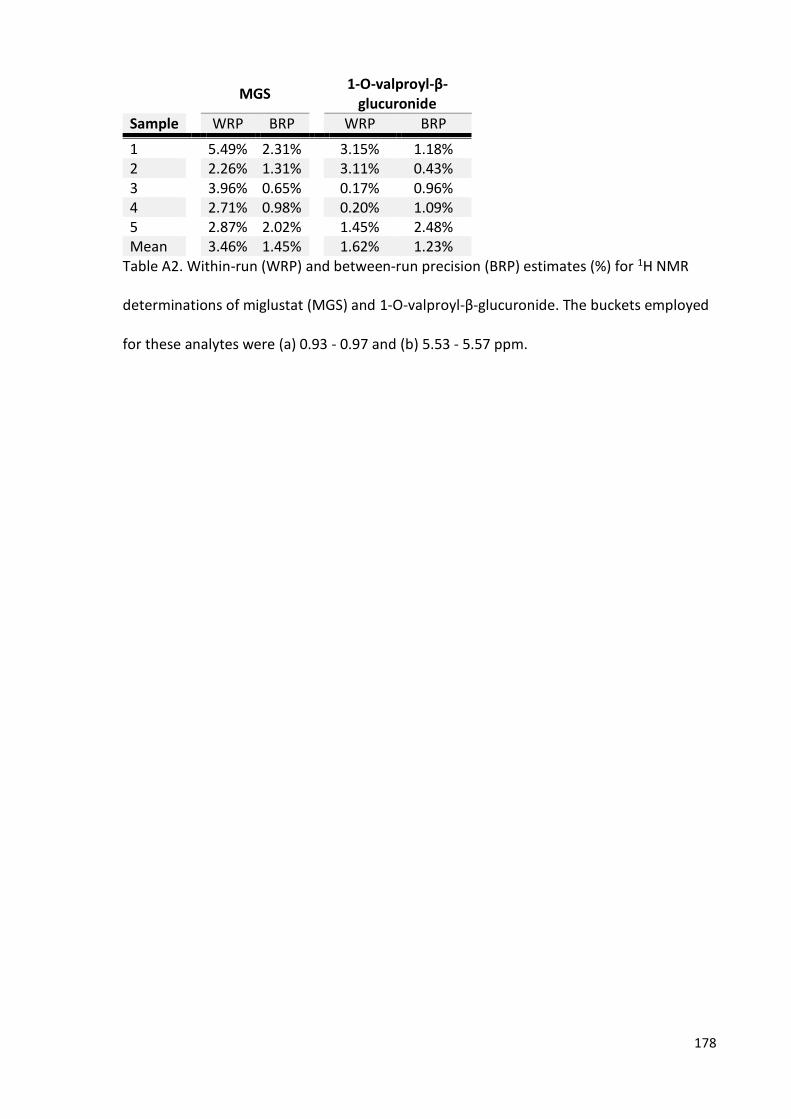
178
MGS
1-O-valproyl-β-glucuronide
Sample WRP BRP WRP BRP
1 5.49% 2.31% 3.15% 1.18% 2 2.26% 1.31% 3.11% 0.43% 3 3.96% 0.65% 0.17% 0.96% 4 2.71% 0.98% 0.20% 1.09% 5 2.87% 2.02% 1.45% 2.48% Mean 3.46% 1.45% 1.62% 1.23%
Table A2. Within-run (WRP) and between-run precision (BRP) estimates (%) for 1H NMR
determinations of miglustat (MGS) and 1-O-valproyl-β-glucuronide. The buckets employed
for these analytes were (a) 0.93 - 0.97 and (b) 5.53 - 5.57 ppm.

179
REFERENCES
1. Rabi II, Millman S, Kusch P, Zacharias JR. The Molecular Beam Resonance Method for Measuring Nuclear Magnetic Moments. The Magnetic Moments of 3Li6, 3Li7 and 9F19. Phys Rev. 1939 Mar;55:526-35.
2. Slicter CP. Principles of Magnetic Resonance. 3rd ed. Heidelberg (Germany): Springer-Verlag; 1990.
3. Keller J. Understanding NMR Spectroscopy. 2nd ed. New Jersey (USA): John Wiley & Sons; 2010.
4. Bloch F, Hansen WW, Packard M. The Nuclear Induction Experiment. Phys Rev. 1946 Oct;70:474-85.
5. Ernst RR, Anderson WA. Application of Fourier transform spectroscopy to magnetic resonance. Rev Sci Instrum. 1966 Dec;37:93-102.
6. Lowe IJ, Norberg RE. Free-Induction Decays in Solids. Phys Rev. 1957 Jul;107:46-61.
7. Kumar A, Ernst RR, Wuthrich K. A two-dimensional nuclear Overhauser enhancement (2D NOE) experiment for the elucidation of complete proton-proton cross-relaxation networks in biological macromolecules. Biochem Biophys Res Commun. 1980 Jul;16;95(1):1-6.
8. Hoult DI. Solvent peak saturation with single phase and quadrature Fourier transformation. J Magn Reson. 1976 Feb;21:337-47.
9. Zheng G, Price WS. Solvent signal suppression in NMR. Prog Nucl Magn Reson Spectrosc. 2010 Apr;56(3):267-88.
10. Ross A, Schlotterbeck G, Dieterle F, Senn H. NMR Spectroscopy Techniques for Application to Metabolomics (55-112).In: The Handbook of Metabonomics and Metabolomics. Lindon JC, Nicholson JK, Holmes E, editors. 1st ed. Amsterdam (The Netherlands): Elsevier Science; 2007.
11. McKay RT. How the 1D-NOESY Suppresses Solvent Signal in Metabonomics NMR Spectroscopy: An Examination of the Pulse Sequence Components and Evolution. Concepts Magn Reson Part A. 2011 Sep;38A(5):197-220.
12. Carr HY, Purcell EM. Effects of diffusion on free precession in nuclear magnetic resonance experiments. Phys Rev. 1954 May;94:630-38.
13. Hahn EL. Spin echoes. Phys Rev. 1950 Nov;80:580-602.

180
14. Meiboom S, Gill DL. Modified spin-echo method for measuring nuclear relaxation times. Rev Sci Instrum. 1958 Aug;29:688-91.
15. Claridge TDW. High-resolution NMR techniques in organic chemistry. 2nd ed. Amsterdam (The Netherlands): Elsevier Science; 2009.
16. Aue WP, Bartholdi E, Ernst RR. Two-dimensional spectroscopy. Application to nuclear magnetic resonance. J Chem Phys. 1976 Mar;64:2229-46.
17. Friebolin H. Basic One- and Two-Dimensional NMR Spectroscopy. 5th ed. New Jersey (USA): John Wiley & Sons; 2011.
18. Braunschweiler L, Ernst RR. Coherence transfer by isotropic mixing: Application to proton correlation spectroscopy J Magn Reson. 1983 Jul;53(3):521-8.
19. Bax A, Davis DG. MLEV-17 based two-dimensional homonuclear magnetization transfer spectroscopy. J Magn Reson. 1985 Jul;65:355-60.
20. Hartmann SR, Hahn EL. Nuclear double resonance in the rotating frame. Phys Rev. 1962 Dec;128(5):2042-53.
21. Roberts JD. ABCs of FT-NMR. 1st ed. Sausalito(USA): University Science Book; 2000.
22. Bodenhausen G, Ruben DJ. Natural abundance nitrogen-15 NMR by enhanced heteronuclear spectroscopy. Chem Phys Lett. 1980 1 Jan;69(1):185-9.
23. Lindon JC, Nicholson JK, Holmes E, Everett JR. Metabonomics: Metabolic processes studied by NMR spectroscopy of biofluids. Concept Magn Res. 2000 Jan;12(5):289-320.
24. Poretsky L. Principles of diabetes mellitus. 2nd ed. New York (USA): Springer; 2010.
25. Jaques J. Greek Medicine from Hippocrates to Galen: Selected papers. 1st ed. Leiden (The Netherlands): Brill ; 2012.
26. Nicholson JK, Wilson ID. Opinion: understanding 'global' systems biology: metabonomics and the continuum of metabolism. Nat Rev Drug Discov. 2003 Aug;2:668-76.
27. Williams RJ. Introduction, General Discussion and Tentative Conclusions. In: Individual metabolic patterns and human disease: an exploratory study utilizing predominantly paper chromatographic methods (7-21). Austin, TX (USA): Biochemical Institute and the Dept. of Chemistry, the University of Texas, and the Clayton Foundation for Research; 1951.
28. Horning MG, Murakami S, Horning EC. Analyses of phospholipids, ceramides, and cerebrosides by gas chromatography and gas chromatography-mass spectrometry. Am J Clin Nutr. 1971 Sep;24(9):1086-96.

181
29. Horning EC, Devaux PG, Moffat AC, Pfaffenberger CD, Sakauchi N, Horning MG. Gas phase analytical separation techniques applicable to problems in clinical chemistry. Clin Chim Acta. 1971 Sep;34(2):135-44.
30. Horning MG, Hung A, Hill RM, Horning EC. Variations in urinary steroid profiles after birth. Clin Chim Acta. 1971 Sep;34(2):261-8.
31. Teranishi R, Mon TR, Robinson AB, Cary P, Pauling L. Gas chromatography of volatiles from breath and urine. Anal Chem. 1972 Jan;44(1):18-20.
32. McConnell ML, Rhodes G, Watson U, Novotny M. Application of pattern recognition and feature extraction techniques to volatile constituent metabolic profiles obtained by capillary gas chromatography. J Chromatogr. 1979 April;162:495-506.
33. Hoult DI, Busby SJ, Gadian DG, Radda GK, Richards RE, Seeley PJ. Observation of tissue metabolites using 31P nuclear magnetic resonance. Nature. 1974 Nov;;252:285-7.
34. Barany M, Barany K, Burt CT, Glonek T, Myers TC. Structural changes in myosin during contraction and the state of ATP in the intact frog muscle. J Supramol Struct. 1975;3(2):125-40.
35. Cheng LL. High-resolution MAS NMR of Tissues and Cells. In: NMR in Pharmaceutical Science (117-28). Everett JR, Harris RK, Lindon JC, Wilson ID, editors.. 1st ed. Singapore (Singapore): Wiley; 2015. p. 117-28.
36. Rabenstein DL. 1H NMR methods for the non-invasive study of metabolism and other processes involving small molecules in intact erythrocytes. J Biochem Biophys Methods. 1984 Sep;9(4):277-306.
37. Brown FF, Campbell ID, Kuchel PW, Rabenstein DC. Human erythrocyte metabolism studies by 1H spin echo NMR. FEBS Lett. 1977 Oct;82(1):12-6.
38. Nicholson JK, Sadler PJ, Bales JR, Juul SM, MacLeod AF, Sonksen PH. Monitoring metabolic disease by proton NMR of urine. Lancet. 1984 Sep;2(8405):751-2.
39. Daniels A, Williams RJ, Wright PE. Nuclear magnetic resonance studies of the adrenal gland and some other organs. Nature. 1976 May;261(5558):321-3.
40. Bock JL. Analysis of serum by high-field proton nuclear magnetic resonance. Clin Chem. 1982 Sep;28(9):1873-7.
41. Arus C, Yen-Chang, Barany M. Proton nuclear magnetic resonance spectra of excised rat brain. Assignment of resonances. Physiol Chem Phys Med NMR. 1985;17(1):23-33.
42. Arus C, Barany M. Application of high-field 1H-NMR spectroscopy for the study of perifused amphibian and excised mammalian muscles. Biochim Biophys Acta. 1986 May 29;886(3):411-24.

182
43. Wishart DS, Tzur D, Knox C, Eisner R, Guo AC, Young N, et al. HMDB: the Human Metabolome Database. Nucleic Acids Res. 2007 Jan;35(Database issue):D521-6.
44. Ulrich EL, Akutsu H, Doreleijers JF, Harano Y, Ioannidis YE, Lin J, et al. BioMagResBank. Nucleic Acids Res. 2008 Jan;36(Database issue):D402-8.
45. Bouatra S, Aziat F, Mandal R, Guo AC, Wilson MR, Knox C, et al. The human urine metabolome. PLoS One. 2013 Sep;8(9):e73076.
46. Psychogios N, Hau DD, Peng J, Guo AC, Mandal R, Bouatra S, et al. The human serum metabolome. PLoS One. 2011 Feb;;6(2):e16957.
47. Dame ZT, Aziat F, Mandal R, Krishnamurthy R, Bouatra S, Borzouie S, et al. The human saliva metabolome. Metabolomics. 2015 Dec;11(6):1864-83.
48. Bingol K, Li DW, Bruschweiler-Li L, Cabrera OA, Megraw T, Zhang F, et al. Unified and isomer-specific NMR metabolomics database for the accurate analysis of (13)C-(1)H HSQC spectra. ACS Chem Biol. 2015 Feb;10(2):452-9.
49. Ravanbakhsh S, Liu P, Bjorndahl TC, Mandal R, Grant JR, Wilson M, et al. Correction: Accurate, Fully-Automated NMR Spectral Profiling for Metabolomics. PLoS One. 2015 Jul ;10(7):e0132873.
50. Xia J, Sinelnikov IV, Han B, Wishart DS. MetaboAnalyst 3.0--making metabolomics more meaningful. Nucleic Acids Res. 2015 Jul;43(W1):W251-7.
51. Emwas AH, Luchinat C, Turano P, Tenori L, Roy R, Salek RM, et al. Standardizing the experimental conditions for using urine in NMR-based metabolomic studies with a particular focus on diagnostic studies: a review. Metabolomics. 2015 Aug;11(4):872-94.
52. Mallol R, Amigo N, Rodriguez MA, Heras M, Vinaixa M, Plana N, et al. Liposcale: a novel advanced lipoprotein test based on 2D diffusion-ordered 1H NMR spectroscopy. J Lipid Res. 2015 Mar;56(3):737-46.
53. Nagana Gowda GA, Raftery D. Quantitating metabolites in protein precipitated serum using NMR spectroscopy. Anal Chem. 2014 Jun;86(11):5433-40.
54. Dona AC, Jimenez B, Schafer H, Humpfer E, Spraul M, Lewis MR, et al. Precision high-throughput proton NMR spectroscopy of human urine, serum, and plasma for large-scale metabolic phenotyping. Anal Chem. 2014 Oct;86(19):9887-94.
55. Salek RM, Steinbeck C, Viant MR, Goodacre R, Dunn WB. The role of reporting standards for metabolite annotation and identification in metabolomic studies. Gigascience. 2013 Oct ;2(1):13,217X-2-13.
56. MSI Board Members, Sansone SA, Fan T, Goodacre R, Griffin JL, Hardy NW, et al. The metabolomics standards initiative. Nat Biotechnol. 2007 Aug;25(8):846-8.
183
57. Emwas AH, Roy R, McKay RT, Ryan D, Brennan L, Tenori L, et al. Recommendations and Standardization of Biomarker Quantification Using NMR-Based Metabolomics with Particular Focus on Urinary Analysis. J Proteome Res. 2016 Feb;15(2):360-73.
58. Pathan M, Akoka S, Tea I, Charrier B, Giraudeau P. "Multi-scan single shot" quantitative 2D NMR: a valuable alternative to fast conventional quantitative 2D NMR. Analyst. 2011 Aug;136(15):3157-63.
59. Le Guennec A, Tea I, Antheaume I, Martineau E, Charrier B, Pathan M, et al. Fast determination of absolute metabolite concentrations by spatially encoded 2D NMR: application to breast cancer cell extracts. Anal Chem. 2012 Dec;84(24):10831-7.
60. Rai RK, Sinha N. Fast and accurate quantitative metabolic profiling of body fluids by nonlinear sampling of 1H-13C two-dimensional nuclear magnetic resonance spectroscopy. Anal Chem. 2012 Nov;84(22):10005-11.
61. Hotelling H. Analysis of a complex of statistical variables into principal components. J Educ Psychol. 1933 Sep;24(6):417-41.
62. Pearson K. On lines and planes of closest fit to systems of points in space. Philos Mag. 1901;2(11):559-72.
63. Rencher AC. Multivariate Statistical Inference and Applications. 1st ed. New Jersey (USA): John Wiley & Sons, Inc; 2002.
64. Abdi H, Williams LJ. Principal component analysis. Wiley Interdiscip Rev Comput Stat. 2010 Jun;2(4):433-59.
65. Kaiser HF. The varimax criterion for analytic rotation in factor analysis. Psychometrika. 1958 Sep;23(3):187-200.
66. Fisher RA. The use of multiple measurements in taxonomic problems. Ann Hum Genet. 1936 Sep;7(2):179-88.
67. Balakrishnam S, Ganapathiraju A. Linear Discriminant Analysis-A Brief Tutorial. Institute for Signal and Information Processing Department of Electrical and Computer Engineering, Mississippi State University. 1998:.
68. Borcard D, Gillet F, Legendre P. Numerical ecology with R. 3rd ed. Oxford (UK): Springer Science & Business Media; 2012.
69. Van den Wollenberg, A. L. Redundancy analysis: An alternative for canonical correlation analysis. Psychometrika. 1977 Jun;42(2):207-19.
70. Davies PT, Tso MK. Procedures for reduced-rank regression. Appl Stat. 1982 Mar;31:244-55.

184
71. Ter Braak CJF. Interpreting canonical correlation analysis through biplots of structure correlations and weights . Psychometrika. 1990 Sep;55(3):519-31.
72. Magidson J. Correlated component regression: re-thinking regression in the presence of near collinearity. In: New Perspectives in Partial Least Squares and Related Methods (65-78). 1st ed. New York (USA): Springer; 2013. p. 65-78.
73. Magidson J. A Fast Parsimonious Maximum Likelihood Approach for Predicting Outcome Variables from a Large Number of Predictors. COMPSTAT 2010 Proceedings; Aug 22-27; Paris; 2010.
74. Magidson J. Correlated Component Regression: A prediction/classification methodology for possibly many featuree. Proceedings of the American Statistical Association.
75. Magidson J, Bennett G. Correlated Component Regression (CCR) - A brief methodological description. 2011.
76. Consonni V, Ballabio D, Todeschini R. Evaluation of model predictive ability by external validation techniques. J Chemometrics. 2010 Feb;24:194-201.
77. Fawcett T. ROC Graphs: Notes and Practical Considerations for Data Mining Researchers. Mach Learn. 2003 Jan;31:1-38.
78. El Khouli RH, Macura KJ, Barker PB, Habba MR, Jacobs MA, Bluemke DA. Relationship of temporal resolution to diagnostic performance for dynamic contrast enhanced MRI of the breast. J Magn Reson Imaging. 2009 Nov;30(5):999-1004.
79. Breiman L. Random Forest. Mach Learn. 2001 Oct;45(1):5-32.
80. De'ath G, Fabricius KE. Classification and regression trees: a powerful yet simple technique for ecological data analysis. Ecology. 2000 Nov;81(11):3178-92.
81. Breiman L, Friedman JH, Olshen RA, Stone CJ. Classification and regression trees. 1st ed. Belmont (USA): Wadsworth & Brooks/Cole; 1984.
82. James G, Witten D, Hastie T, Tibshirani R. The Bootstrap. In: An introduction to statistical learning (187-90). 6th ed. New York (USA): Springer; 2013.
83. Felsenstein J. Confidence limits on phylogenies: an approach using the bootstrap. Evolution. 1985 Jul;39(4):783-91.
84. Efron B, Gong G. A leisurely look at the bootstrap the jackknife, and cross validation. Am Stat. 1983 Feb;37(1):36-48.
85. Vapnik V. Estimation of Dependences Based on Empirical Data. 1st ed. New York (USA): Springer Verlag; 1982.

185
86. Boser BE, Guyon IM, Vapnik VN. A training algorithm for optimal margin classifiers. In: Proceedings of the fifth annual workshop on Computational learning theory (144-52), ACM. 1992.
87. Vapnik V. Statistical Learning Theory. 1st ed. New York (USA): John Wiley and Sons, Inc; 1998.
88. Holland JH. Adaptation in Natural and Artificial Systems. 1st ed. Michigan (USA): University of Michigan Press; 1975.
89. Srinivas M, Patnaik LM. Adaptive probabilities of crossover and mutation in genetic algorithms. IEEE Trans Syst Man Cybern. 1994 Apr;24(4):656-67.
90. Lin X, Wang Q, Yin P. A method for handling metabonomics data from liquid chromatography/mass spectrometry: combinational use of support vector machine recursive feature elimination, genetic algorithm and random forest for feature selection. Metabolomics. 2011 Dec;7(4):549-58.
91. Vanier MT. Niemann-Pick disease type C. Orphanet J Rare Dis. 2010 Jun;5:16,1172-5-16.
92. Vanier MT, Millat G. Niemann-Pick disease type C. Clin Genet. 2003 Sep;64:269-81.
93. Sun X, Marks DL, Park WD, Wheatley CL, Puri V, O'Brien JF, et al. Niemann-Pick C variant detection by altered sphingolipid trafficking and correlation with mutations within a specific domain of NPC1. Am J Hum Genet. 2001 Jun;68(6):1361-72.
94. Sturley SL, Patterson MC, Balch W, Liscum L. The pathophysiology and mechanisms of NP-C disease. Biochim Biophys Acta. 2004 Oct;1685(1-3):83-7.
95. NP-C Guidelines Working Group, Wraith JE, Baumgartner MR, Bembi B, Covanis A, Levade T, et al. Recommendations on the diagnosis and management of Niemann-Pick disease type C. Mol Genet Metab. 2009 Sep-Oct;98(1-2):152-65.
96. Vance DE, Van den Bosch H. Cholesterol in the year 2000. Biochim Biophys Acta. 2000 Dec;1529(1-3):1-8.
97. Jurevics H, Morell P. Cholesterol for synthesis of myelin is made locally, not imported into brain. J Neurochem. 1995 Feb;64(2):895-901.
98. Riobo NA. Cholesterol and its derivatives in Sonic Hedgehog signaling and cancer. Curr Opin Pharmacol. 2012 Dec;12(6):736-41.
99. Briscoe J, Therond PP. The mechanisms of Hedgehog signalling and its roles in development and disease. Nat Rev Mol Cell Biol. 2013 Jul;14(7):416-29.
100. Weedon MN, Lango H, Lindgren CM, Wallace C, Evans DM, Mangino M, et al. Genome-wide association analysis identifies 20 loci that influence adult height. Nat Genet. 2008 May;40(5):575-83.
186
101. Ahn S, Joyner AL. In vivo analysis of quiescent adult neural stem cells responding to Sonic hedgehog. Nature. 2005 Oct;437(7060):894-7.
102. Oram JF, Vaughan AM. ATP-Binding cassette cholesterol transporters and cardiovascular disease. Circ Res. 2006 Nov;99(10):1031-43.
103. Liscum L, Munn NJ. Intracellular cholesterol transport. Biochim Biophys Acta. 1999 Apr;1438(1):19-37.
104. Vance JE. Dysregulation of cholesterol balance in the brain: contribution to neurodegenerative diseases. Dis Model Mech. 2012 Nov;5(6):746-55.
105. Bjorkhem I. Crossing the barrier: oxysterols as cholesterol transporters and metabolic modulators in the brain. J Intern Med. 2006 Dec;260(6):493-508.
106. Ikonen E. Cellular cholesterol trafficking and compartmentalization. Nat Rev Mol Cell Biol. 2008 Feb;9(2):125-38.
107. Karten B, Peake KB, Vance JE. Mechanisms and consequences of impaired lipid trafficking in Niemann-Pick type C1-deficient mammalian cells. Biochim Biophys Acta. 2009 Jul;1791(7):659-70.
108. Storch J, Xu Z. Niemann-Pick C2 (NPC2) and intracellular cholesterol trafficking. Biochim Biophys Acta. 2009 Jul;1791(7):671-8.
109. Peake KB, Vance JE. Defective cholesterol trafficking in Niemann-Pick C-deficient cells. FEBS Lett. 2010 Jul;584(13):2731-9.
110. Zhou S, Davidson C, McGlynn R, Stephney G, Dobrenis K, Vanier MT, et al. Endosomal/lysosomal processing of gangliosides affects neuronal cholesterol sequestration in Niemann-Pick disease type C. Am J Pathol. 2011 Aug;179(2):890-902.
111. Platt N, Speak AO, Colaco A, Gray J, Smith DA, Williams IM, et al. Immune dysfunction in Niemann-Pick disease type C. J Neurochem. 2015 Jan; 136 Suppl 1:74-80.
112. Stampfer M, Theiss S, Amraoui Y, Jiang X, Keller S, Ory DS, et al. Niemann-Pick disease type C clinical database: cognitive and coordination deficits are early disease indicators. Orphanet J Rare Dis. 2013 Feb;8:35,1172-8-35.
113. Sevin M, Lesca G, Baumann N, Millat G, Lyon-Caen O, Vanier MT, et al. The adult form of Niemann-Pick disease type C. Brain. 2007 Jan;130(Pt 1):120-33.
114. Madra M, Sturley SL. Niemann-Pick type C pathogenesis and treatment: from statins to sugars. Clin Lipidol. 2010 Jun;5(3):387-95.
115. Pineda M, Wraith JE, Mengel E, Sedel F, Hwu WL, Rohrbach M, et al. Miglustat in patients with Niemann-Pick disease Type C (NP-C): a multicenter observational retrospective cohort study. Mol Genet Metab. 2009 Nov;98(3):243-9.
187
116. Mengel E, Klunemann HH, Lourenco CM, Hendriksz CJ, Sedel F, Walterfang M, et al. Niemann-Pick disease type C symptomatology: an expert-based clinical description. Orphanet J Rare Dis. 2013 Oct;8:166,1172-8-166.
117. Wijburg FA, Sedel F, Pineda M, Hendriksz CJ, Fahey M, Walterfang M, et al. Development of a suspicion index to aid diagnosis of Niemann-Pick disease type C. Neurology. 2012 May;78(20):1560-7.
118. Kelly DA, Portmann B, Mowat AP, Sherlock S, Lake BD. Niemann-Pick disease type C: diagnosis and outcome in children, with particular reference to liver disease. J Pediatr. 1993 Aug;123(2):242-7.
119. Mieli-Vergani G, Howard ER, Mowat AP. Liver disease in infancy: a 20 year perspective. Gut. 1991 Sep;Suppl:S123-8.
120. Yerushalmi B, Sokol RJ, Narkewicz MR, Smith D, Ashmead JW, Wenger DA. Niemann-pick disease type C in neonatal cholestasis at a North American Center. J Pediatr Gastroenterol Nutr. 2002 Jul;35(1):44-50.
121. Garver WS, Jelinek D, Oyarzo JN, Flynn J, Zuckerman M, Krishnan K, et al. Characterization of liver disease and lipid metabolism in the Niemann-Pick C1 mouse. J Cell Biochem. 2007 May;101(2):498-516.
122. Beltroy EP, Richardson JA, Horton JD, Turley SD, Dietschy JM. Cholesterol accumulation and liver cell death in mice with Niemann-Pick type C disease. Hepatology. 2005 Oct;42(4):886-93.
123. Cluzeau CV, Watkins-Chow DE, Fu R, Borate B, Yanjanin N, Dail MK, et al. Microarray expression analysis and identification of serum biomarkers for Niemann-Pick disease, type C1. Hum Mol Genet. 2012 Aug;21(16):3632-46.
124. Loftus SK, Morris JA, Carstea ED, Gu JZ, Cummings C, Brown A, et al. Murine model of Niemann-Pick C disease: mutation in a cholesterol homeostasis gene. Science. 1997 Jul;277(5323):232-5.
125. Erickson RP, Bhattacharyya A, Hunter RJ, Heidenreich RA, Cherrington NJ. Liver disease with altered bile acid transport in Niemann-Pick C mice on a high-fat, 1% cholesterol diet. Am J Physiol Gastrointest Liver Physiol. 2005 Aug;289(2):G300-7.
126. McKay Bounford K, Gissen P. Genetic and laboratory diagnostic approach in Niemann Pick disease type C. J Neurol. 2014 Sep;261 Suppl 2:S569-75.
127. Bornig H, Geyer G. Staining of cholesterol with the fluorescent antibiotic "filipin". Acta Histochem. 1974 Feb;50(1):110-5.
128. Takamura A, Sakai N, Shinpoo M, Noguchi A, Takahashi T, Matsuda S, et al. The useful preliminary diagnosis of Niemann-Pick disease type C by filipin test in blood smear. Mol Genet Metab. 2013 Nov;110(3):401-4.

188
129. Vanier MT, Latour P. Laboratory diagnosis of Niemann-Pick disease type C: the filipin staining test. Methods Cell Biol. 2015 Jan;126:357-75.
130. Jiang X, Sidhu R, Porter FD, Yanjanin NM, Speak AO, te Vruchte DT. A sensitive and specific LC-MS/MS method for rapid diagnosis of NiemannPick C1 disease from human plasma. J Lipid Res. 2011 Jul;52(7):1435-45.
131. te Vruchte D, Speak AO, Wallom KL, Al Eisa N, Smith DA, Hendriksz CJ, et al. Relative acidic compartment volume as a lysosomal storage disorder-associated biomarker. J Clin Invest. 2014 Mar;124(3):1320-8.
132. Giese AK, Mascher H, Grittner U, Eichler S, Kramp G, Lukas J, et al. A novel, highly sensitive and specific biomarker for Niemann-Pick type C1 disease. Orphanet J Rare Dis. 2015 Jun;10:78,015-0274-1.
133. Sedel F, Barnerias C, Dubourg O, Desguerres I, Lyon-Caen O, Saudubray JM. Peripheral neuropathy and inborn errors of metabolism in adults. J Inherit Metab Dis. 2007 Oct;30(5):642-53.
134. Sandu S, Jackowski-Dohrmann S, Ladner A, Haberhausen M, Bachmann C. Niemann-Pick disease type C1 presenting with psychosis in an adolescent male. Eur Child Adolesc Psychiatry. 2009 Sep;18(9):583-5.
135. Heron B, Valayannopoulos V, Baruteau J, Chabrol B, Ogier H, Latour P, et al. Miglustat therapy in the French cohort of paediatric patients with Niemann-Pick disease type C. Orphanet J Rare Dis. 2012 Jun;7:36,1172-7-36.
136. Helquist P, Maxfield FR, Wiech NL, Wiest O. Treatment of Niemann--pick type C disease by histone deacetylase inhibitors. Neurotherapeutics. 2013 Oct;10(4):688-97.
137. Alvarez AR, Klein A, Castro J, Cancino GI, Amigo J, Mosqueira M, et al. Imatinib therapy blocks cerebellar apoptosis and improves neurological symptoms in a mouse model of Niemann-Pick type C disease. FASEB J. 2008 Oct;22(10):3617-27.
138. Davidson CD, Ali NF, Micsenyi MC, Stephney G, Renault S, Dobrenis K, et al. Chronic cyclodextrin treatment of murine Niemann-Pick C disease ameliorates neuronal cholesterol and glycosphingolipid storage and disease progression. PLoS One. 2009 Sep;4(9):e6951.
139. Liu B, Turley SD, Burns DK, Miller AM, Repa JJ, Dietschy JM. Reversal of defective lysosomal transport in NPC disease ameliorates liver dysfunction and neurodegeneration in the npc1-/- mouse. Proc Natl Acad Sci U S A. 2009 Feb;106(7):2377-82.
140. Pipalia NH, Cosner CC, Huang A, Chatterjee A, Bourbon P, Farley N, et al. Histone deacetylase inhibitor treatment dramatically reduces cholesterol accumulation in Niemann-Pick type C1 mutant human fibroblasts. Proc Natl Acad Sci U S A. 2011 Apr;108(14):5620-5.

189
141. Smith D, Wallom KL, Williams IM, Jeyakumar M, Platt FM. Beneficial effects of anti-inflammatory therapy in a mouse model of Niemann-Pick disease type C1. Neurobiol Dis. 2009 Nov;36(2):242-51.
142. Williams IM, Wallom KL, Smith DA, Al Eisa N, Smith C, Platt FM. Improved neuroprotection using miglustat, curcumin and ibuprofen as a triple combination therapy in Niemann-Pick disease type C1 mice. Neurobiol Dis. 2014 Jul;67:9-17.
143. Wada R, Tifft CJ, Proia RL. Microglial activation precedes acute neurodegeneration in Sandhoff disease and is suppressed by bone marrow transplantation. Proc Natl Acad Sci U S A. 2000 Sep;97(20):10954-9.
144. Stein VM, Crooks A, Ding W, Prociuk M, O'Donnell P, Bryan C, et al. Miglustat improves purkinje cell survival and alters microglial phenotype in feline Niemann-Pick disease type C. J Neuropathol Exp Neurol. 2012 May;71(5):434-48.
145. Butters TD, Dwek RA, Platt FM. Inhibition of glycosphingolipid biosynthesis: application to lysosomal storage disorders. Chem Rev. 2000 Nov;100:4683-96.
146. Ribas GS, Pires R, Coelho JC, Rodrigues D, Mescka CP, Vanzin CS, et al. Oxidative stress in Niemann-Pick type C patients: a protective role of N-butyl-deoxynojirimycin therapy. Int J Dev Neurosci. 2012 Oct;30(6):439-44.
147. Fu R, Yanjanin NM, Bianconi S, Pavan WJ, Porter FD. Oxidative stress in Niemann-Pick disease, type C. Mol Genet Metab. 2010 Oct-Nov;101(2-3):214-8.
148. Mattsson N, Zetterberg H, Bianconi S, Yanjanin NM, Fu R, Mansson JE, et al. Miglustat treatment may reduce cerebrospinal fluid levels of the axonal degeneration marker tau in niemann-pick type C. JIMD Rep. 2011 Sep;3:45-52.
149. Jeyakumar M, Butters TD, Cortina-Borja M, Hunnam V, Proia RL, Perry VH, et al. Delayed symptom onset and increased life expectancy in Sandhoff disease mice treated with N-butyldeoxynojirimycin. Proc Natl Acad Sci U S A. 1999 May;96(11):6388-93.
150. Cox T, Lachmann R, Hollak C, Aerts J, van Weely S, Hrebicek M, et al. Novel oral treatment of Gaucher's disease with N-butyldeoxynojirimycin (OGT 918) to decrease substrate biosynthesis. Lancet. 2000 Apr;355(9214):1481-5.
151. Lachmann RH. Miglustat. Oxford GlycoSciences/Actelion. Curr Opin Investig Drugs. 2003 Apr;4(4):472-9.
152. Di Rocco M, Dardis A, Madeo A, Barone R, Fiumara A. Early miglustat therapy in infantile Niemann-Pick disease type C. Pediatr Neurol. 2012 Jul;47(1):40-3.
153. Zervas M, Somers KL, Thrall MA, Walkley SU. Critical role for glycosphingolipids in Niemann-Pick disease type C. Curr Biol. 2001 Aug;11(16):1283-7.

190
154. Rottach KG, von Maydell RD, Das VE, Zivotofsky AZ, Discenna AO, Gordon JL, et al. Evidence for independent feedback control of horizontal and vertical saccades from Niemann-Pick type C disease. Vision Res. 1997 Dec;37(24):3627-38.
155. Solomon D, Winkelman AC, Zee DS, Gray L, Buttner-Ennever J. Niemann-Pick type C disease in two affected sisters: ocular motor recordings and brain-stem neuropathology. Ann N Y Acad Sci. 2005 Apr;1039:436-45.
156. Neville BG, Lake BD, Stephens R, Sanders MD. A neurovisceral storage disease with vertical supranuclear ophthalmoplegia, and its relationship to Niemann-Pick disease: A report of nine patients. Brain. 1973 Mar;96(1):97-120.
157. Patterson MC, Vecchio D, Prady H, Abel L, Wraith JE. Miglustat for treatment of Niemann-Pick C disease: a randomised controlled study. Lancet Neurol. 2007 Sep;6(9):765-72.
158. Wraith JE, Vecchio D, Jacklin E, Lucy R, Giorgino R, Patterson MC. Disease stability in patients with Niemann-Pick disease type C treated with Miglustat, in: Lysosomal Diseases Network WORLD Symposium, San Diego, California, USA, 2009.
159. Salek RM, Maguire ML, Bentley E, Rubtsov DV, Hough T, Cheeseman M, et al. A metabolomic comparison of urinary changes in type 2 diabetes in mouse, rat, and human. Physiol Genomics. 2007 Apr;29(2):99-108.
160. Martin FP, Dumas ME, Wang Y, Legido-Quigley C, Yap IK, Tang H, et al. A top-down systems biology view of microbiome-mammalian metabolic interactions in a mouse model. Mol Syst Biol. 2007 May;3:112.
161. Wishart DS, Jewison T, Guo AC, Wilson M, Knox C, Liu Y, et al. HMDB 3.0--The Human Metabolome Database in 2013. Nucleic Acids Res. 2013 Jan;41(Database issue):D801-7.
162. Hofmann AF, Mysels KJ. Bile acid solubility and precipitation in vitro and in vivo: the role of conjugation, pH, and Ca2+ ions. J Lipid Res. 1992 May;33(5):617-26.
163. Viau C, Lafontaine M, Payan JP. Creatinine normalization in biological monitoring revisited: the case of 1-hydroxypyrene. Int Arch Occup Environ Health. 2004 Apr;77(3):177-85.
164. Heavner DL, Morgan WT, Sears SB, Richardson JD, Byrd GD, Ogden MW. Effect of creatinine and specific gravity normalization techniques on xenobiotic biomarkers in smokers' spot and 24-h urines. J Pharm Biomed Anal. 2006 Mar;40(4):928-42.
165. Liaw A, Wiener M. Classification and regression by randomForest. R. News 2002. 2:18-22.
166. Trevino V, Falciani F. GALGO: an R package for multivariate variable selection using genetic algorithms. Bioinformatics. 2006 May;22(9):1154-6.
191
167. Li M, Wang B, Zhang M, Rantalainen M, Wang S, Zhou H, et al. Symbiotic gut microbes modulate human metabolic phenotypes. Proc Natl Acad Sci U S A. 2008 Feb;105(6):2117-22.
168. Kemsley EK, Le Gall G, Dainty JR, Watson AD, Harvey LJ, Tapp HS, et al. Multivariate techniques and their application in nutrition: a metabolomics case study. Br J Nutr. 2007 Jul;98(1):1-14.
169. Xia J, Broadhurst DI, Wilson M, Wishart DS. Translational biomarker discovery in clinical metabolomics: an introductory tutorial. Metabolomics. 2013 Apr;9(2):280-99.
170. Kawai T, Yasugi T, Mizunuma K, Horiguchi S, Hirase Y, Uchida Y, et al. Methanol in urine as a biological indicator of occupational exposure to methanol vapor. Int Arch Occup Environ Health. 1991 Oct;63(5):311-8.
171. Slupsky CM, Rankin KN, Wagner J, Fu H, Chang D, Weljie AM, et al. Investigations of the effects of gender, diurnal variation, and age in human urinary metabolomic profiles. Anal Chem. 2007 Sep;79(18):6995-7004.
172. Rebouche CJ. Kinetics, pharmacokinetics, and regulation of L-carnitine and acetyl-L-carnitine metabolism. Ann N Y Acad Sci. 2004 Nov;1033:30-41.
173. Zuppi C, Messana I, Forni F, Ferrari F, Rossi C, Giardina B. Influence of feeding on metabolite excretion evidenced by urine 1H NMR spectral profiles: a comparison between subjects living in Rome and subjects living at arctic latitudes (Svaldbard). Clin Chim Acta. 1998 Nov;278(1):75-9.
174. Solanky KS, Bailey NJ, Beckwith-Hall BM, Bingham S, Davis A, Holmes E, et al. Biofluid 1H NMR-based metabonomic techniques in nutrition research - metabolic effects of dietary isoflavones in humans. J Nutr Biochem. 2005 Apr;16(4):236-44.
175. Lukaski HC. Methods for the assessment of human body composition: traditional and new. Am J Clin Nutr. 1987 Oct;46(4):537-56.
176. Roche AF, Heymsfield SB, Lohma TG. Human body composition. 1st ed. Champaign (USA): Human Kinetics Publishers; 1996.
177. Selberg O, Sel S. The adjunctive value of routine biochemistry in nutritional assessment of hospitalized patients. Clin Nutr. 2001 Dec;20(6):477-85.
178. Azaroual N, Imbenotte M, Cartigny B, Leclerc F, Vallee L, Lhermitte M, et al. Valproic acid intoxication identified by 1H and 1H-(13)C correlated NMR spectroscopy of urine samples. MAGMA. 2000 Jul;10(3):177-82.
179. Meshitsuka S, Koeda T, Muro H. Direct observation of 3-keto-valproate in urine by 2D-NMR spectroscopy. Clin Chim Acta. 2003 Aug;334(1-2):145-51.
192
180. Booth CL, Pollack GM, Brouwer KL. Hepatobiliary disposition of valproic acid and valproate glucuronide: use of a pharmacokinetic model to examine the rate-limiting steps and potential sites of drug interactions. Hepatology. 1996 Apr;23(4):771-80.
181. Fisher E, Siemes H, Pund R, Wittfoht W, Nau H. Valproate metabolites in serum and urine during antiepileptic therapy in children with infantile spasms: abnormal metabolite pattern associated with reversible hepatotoxicity. Epilepsia. 1992 Jan-Feb;33(1):165-71.
182. Guitton J, Coste S, Guffon-Fouilhoux N, Cohen S, Manchon M, Guillaumont M. Rapid quantification of miglustat in human plasma and cerebrospinal fluid by liquid chromatography coupled with tandem mass spectrometry. J Chromatogr B Analyt Technol Biomed Life Sci. 2009 Jan;877(3):149-54.
183. Spieker E, Wagner-Redeker W, Dingemanse J. Validated LC-MS/MS method for the quantitative determination of the glucosylceramide synthase inhibitor miglustat in mouse plasma and human plasma and its application to a pharmacokinetic study. J Pharm Biomed Anal. 2012 Feb;59:123-9.
184. Lachmann RH, te Vruchte D, Lloyd-Evans E, Reinkensmeier G, Sillence DJ, Fernandez-Guillen L, et al. Treatment with miglustat reverses the lipid-trafficking defect in Niemann-Pick disease type C. Neurobiol Dis. 2004 Aug;16(3):654-8.
185. Treiber A, Morand O, Clozel M. The pharmacokinetics and tissue distribution of the glucosylceramide synthase inhibitor miglustat in the rat. Xenobiotica. 2007 Mar;37(3):298-314.
186. Gao S, Miao H, Tao X, Jiang B, Xiao Y, Cai F, et al. LC-MS/MS method for simultaneous determination of valproic acid and major metabolites in human plasma. J Chromatogr B Analyt Technol Biomed Life Sci. 2011 Jul;879(21):1939-44.
187. Argikar UA, Remmel RP. Effect of aging on glucuronidation of valproic acid in human liver microsomes and the role of UDP-glucuronosyltransferase UGT1A4, UGT1A8, and UGT1A10. Drug Metab Dispos. 2009 Jan;37(1):229-36.
188. Proenca P, Franco JM, Mustra C, Marcos M, Pereira AR, Corte-Real F, et al. An UPLC-MS/MS method for the determination of valproic acid in blood of a fatal intoxication case. J Forensic Leg Med. 2011 Oct;18(7):320-4.
189. Chen ZJ, Wang XD, Wang HS, Chen SD, Zhou LM, Li JL, et al. Simultaneous determination of valproic acid and 2-propyl-4-pentenoic acid for the prediction of clinical adverse effects in Chinese patients with epilepsy. Seizure. 2012 Mar;21(2):110-7.
190. Lyseng-Williamson KA. Miglustat: a review of its use in Niemann-Pick disease type C. Drugs. 2014 Jan;74(1):61-74.
191. Chen S, Beaton D, Nguyen N, Senekeo-Effenberger K, Brace-Sinnokrak E, Argikar U, et al. Tissue-specific, inducible, and hormonal control of the human UDP-glucuronosyltransferase-1 (UGT1) locus. J Biol Chem. 2005 Nov;280(45):37547-57.

193
192. Nicholson JK. Global systems biology, personalized medicine and molecular epidemiology. Mol Syst Biol. 2006 Oct;2:52-58.
193. Crockford DJ, Maher AD, Ahmadi KR, Barrett A, Plumb RS, Wilson ID, et al. 1H NMR and UPLC-MS(E) statistical heterospectroscopy: characterization of drug metabolites (xenometabolome) in epidemiological studies. Anal Chem. 2008 Sep;80(18):6835-44.
194. Elstein D, Dweck A, Attias D, Hadas-Halpern I, Zevin S, Altarescu G, et al. Oral maintenance clinical trial with miglustat for type I Gaucher disease: switch from or combination with intravenous enzyme replacement. Blood. 2007 Oct;110(7):2296-301.
195. Kuter DJ, Mehta A, Hollak CE, Giraldo P, Hughes D, Belmatoug N, et al. Miglustat therapy in type 1 Gaucher disease: clinical and safety outcomes in a multicenter retrospective cohort study. Blood Cells Mol Dis. 2013 Aug;51(2):116-24.
196. Patterson MC, Vecchio D, Jacklin E, Abel L, Chadha-Boreham H, Luzy C, et al. Long-term miglustat therapy in children with Niemann-Pick disease type C. 2010 Mar;25:300-5.
197. Iturriaga C, Pineda M, Fernandez-Valero EM, Vanier MT, Coll MJ. Niemann-Pick C disease in Spain: clinical spectrum and development of a disability scale. J Neurol Sci. 2006 Nov;249(1):1-6.
198. Elstein D, Hollak C, Aerts JM, van Weely S, Maas M, Cox TM, et al. Sustained therapeutic effects of oral miglustat (Zavesca, N-butyldeoxynojirimycin, OGT 918) in type I Gaucher disease. J Inherit Metab Dis. 2004 Nov;27(6):757-66.
199. Santos ML, Raskin S, Telles DS, Lohr A,Jr, Liberalesso PB, Vieira SC, et al. Treatment of a child diagnosed with Niemann-Pick disease type C with miglustat: a case report in Brazil. J Inherit Metab Dis. 2008 Dec;31 Suppl 2:S357-61.
200. Chien YH, Lee NC, Tsai LK, Huang AC, Peng SF, Chen SJ, et al. Treatment of Niemann-Pick disease type C in two children with miglustat: initial responses and maintenance of effects over 1 year. J Inherit Metab Dis. 2007 Oct;30(5):826.
201. Platt FM, Boland B, van der Spoel AC. The cell biology of disease: lysosomal storage disorders: the cellular impact of lysosomal dysfunction. J Cell Biol. 2012 Nov;199(5):723-34.
202. Rosenbaum AI, Maxfield FR. Niemann-Pick type C disease: molecular mechanisms and potential therapeutic approaches. J Neurochem. 2011 Mar;116(5):789-95.
203. Engelke UF, Liebrand-van Sambeek ML, de Jong JG, Leroy JG, Morava E, Smeitink JA, et al. N-acetylated metabolites in urine: proton nuclear magnetic resonance spectroscopic study on patients with inborn errors of metabolism. Clin Chem. 2004 Jan;50(1):58-66.
204. Aerts JM, Hollak CE, Boot RG, Groener JE, Maas M. Substrate reduction therapy of glycosphingolipid storage disorders. J Inherit Metab Dis. 2006 Apr-Jun;29(2-3):449-56.

194
205. Lopez ME, Klein AD, Hong J, Dimbil UJ, Scott MP. Neuronal and epithelial cell rescue resolves chronic systemic inflammation in the lipid storage disorder Niemann-Pick C. Hum Mol Genet. 2012 Jul;21(13):2946-60.
206. Merrifield CA, Lewis M, Claus SP, Beckonert OP, Dumas ME, Duncker S, et al. A metabolic system-wide characterisation of the pig: a model for human physiology. Mol Biosyst. 2011 Sep;7(9):2577-88.
207. Soininen P, Kangas AJ, Wurtz P, Tukiainen T, Tynkkynen T, Laatikainen R, et al. High-throughput serum NMR metabonomics for cost-effective holistic studies on systemic metabolism. Analyst. 2009 Sep;134(9):1781-5.
208. Nicholson JK, Foxall PJ, Spraul M, Farrant RD, Lindon JC. 750 MHz 1H and 1H-13C NMR spectroscopy of human blood plasma. Anal Chem. 1995 Mar;67(5):793-811.
209. Barton RH, Waterman D, Bonner FW, Holmes E, Clarke R, Procardis Consortium, et al. The influence of EDTA and citrate anticoagulant addition to human plasma on information recovery from NMR-based metabolic profiling studies. Mol Biosyst. 2010 Jan;6(1):215-24.
210. Sidhu D, Naugler C. Fasting time and lipid levels in a community-based population: a cross-sectional study. Arch Intern Med. 2012 Dec;172(22):1707-10.
211. te Vruchte D, Lloyd-Evans E, Veldman RJ, Neville DC, Dwek RA, Platt FM, et al. Accumulation of glycosphingolipids in Niemann-Pick C disease disrupts endosomal transport. J Biol Chem. 2004 Jun;279(25):26167-75.
212. Waters NJ, Holmes E, Williams A, Waterfield CJ, Farrant RD, Nicholson JK. NMR and pattern recognition studies on the time-related metabolic effects of alpha-naphthylisothiocyanate on liver, urine, and plasma in the rat: an integrative metabonomic approach. Chem Res Toxicol. 2001 Oct;14(10):1401-12.
213. Smilde AK, Jansen JJ, Hoefsloot HC, Lamers RJ, van der Greef J, Timmerman ME. ANOVA-simultaneous component analysis (ASCA): a new tool for analyzing designed metabolomics data. Bioinformatics. 2005 May;21(13):3043-8.
214. Townsend DM, Tew KD, Tapiero H. The importance of glutathione in human disease. Biomed Pharmacother. 2003 May-Jun;57(3-4):145-55.
215. Schafer FQ, Buettner GR. Redox environment of the cell as viewed through the redox state of the glutathione disulfide/glutathione couple. Free Radic Biol Med. 2001 Jun;30(11):1191-212.
216. Fan TW, Lane AN, Higashi RM, Farag MA, Gao H, Bousamra M, et al. Altered regulation of metabolic pathways in human lung cancer discerned by (13)C stable isotope-resolved metabolomics (SIRM). Mol Cancer. 2009 Jun;8:41,4598-8-41.
217. Fan TW, Lane AN. NMR-based stable isotope resolved metabolomics in systems biochemistry. J Biomol NMR. 2011 Apr;49(3-4):267-80.
195
218. Diaz-Uriarte R, Alvarez de Andres S. Gene selection and classification of microarray data using random forest. BMC Bioinformatics. 2006 Jan;7(1):1-13.
219. Saeys Y, Inza I, Larranaga P. A review of feature selection techniques in bioinformatics. 2007 Aug;23:2507-17.
220. Hastie T, Tibshirani R, Friedman J. The Elements of Statistical Learning: Data Mining, Inference and Prediction. 2nd ed. New York (USA): Springer-Verlag; 2009.
221. Bertini I, Luchinat C, Miniati M, Monti S, Tenori L. Phenotyping COPD by 1H NMR metabolomics of exhaled breath condensate. Metabolomics. 2014 Apr;10(2):302-11.
222. Smolinska A, Klaassen EM, Dallinga JW, van de Kant KD, Jobsis Q, Moonen EJ, et al. Profiling of volatile organic compounds in exhaled breath as a strategy to find early predictive signatures of asthma in children. PLoS One. 2014 Apr;9(4):e95668.
223. Bureau A, Dupuis J, Hayward B, Falls K, Van Eerdewegh P. Mapping complex traits using Random Forests. BMC Genet. 2003 Dec;4 Suppl 1:S64.
224. Strobl C, Boulesteix AL, Zeileis A, Hothorn T. Bias in random forest variable importance measures: illustrations, sources and a solution. BMC Bioinform. 2007 Jan;8(1):1-25.
225. Bao L, Cui Y. Prediction of the phenotypic effects of non-synonymous single nucleotide polymorphisms using structural and evolutionary information. Bioinformatics. 2005 May;21(10):2185-90.
226. Genuer R, Poggi JM, Tuleau-Malot C. Variable selection using random forests. Pattern Recogn Lett. 2010 Oct;31(14):2225-36.
227. Hara N, Yamada K, Shibata T, Osago H, Hashimoto T, Tsuchiya M. Elevation of cellular NAD levels by nicotinic acid and involvement of nicotinic acid phosphoribosyltransferase in human cells. J Biol Chem. 2007 Aug;282(34):24574-82.
228. Lushchak VI. Glutathione homeostasis and functions: potential targets for medical interventions. J Amino Acids. 2012 Jan;2012:736837.
229. Penke M, Larsen PS, Schuster S, Dall M, Jensen BA, Gorski T, et al. Hepatic NAD salvage pathway is enhanced in mice on a high-fat diet. Mol Cell Endocrinol. 2015 Sep;412:65-72.
230. Chang WC, Jia H, Aw W, Saito K, Hasegawa S, Kato H. Beneficial effects of soluble dietary Jerusalem artichoke (Helianthus tuberosus) in the prevention of the onset of type 2 diabetes and non-alcoholic fatty liver disease in high-fructose diet-fed rats. Br J Nutr. 2014 Sep;112(5):709-17.
231. Kukla M, Ciupinska-Kajor M, Kajor M, Wylezol M, Zwirska-Korczala K, Hartleb M, et al. Liver visfatin expression in morbidly obese patients with nonalcoholic fatty liver disease undergoing bariatric surgery. Pol J Pathol. 2010;61(3):147-53.
196
232. Koliaki C, Roden M. Hepatic energy metabolism in human diabetes mellitus, obesity and non-alcoholic fatty liver disease. Mol Cell Endocrinol. 2013 Oct;379(1-2):35-42.
233. Jelinek DA, Maghsoodi B, Borbon IA, Hardwick RN, Cherrington NJ, Erickson RP. Genetic variation in the mouse model of Niemann Pick C1 affects female, as well as male, adiposity, and hepatic bile transporters but has indeterminate effects on caveolae. Gene. 2012 Jan;491(2):128-34.
234. Magni G, Amici A, Emanuelli M, Orsomando G, Raffaelli N, Ruggieri S. Enzymology of NAD+ homeostasis in man. Cell Mol Life Sci. 2004 Jan;61(1):19-34.
235. Moffett JR, Namboodiri MA. Tryptophan and the immune response. Immunol Cell Biol. 2003 Aug;81(4):247-65.
236. Guillemin GJ, Kerr SJ, Smythe GA, Smith DG, Kapoor V, Armati PJ, et al. Kynurenine pathway metabolism in human astrocytes: a paradox for neuronal protection. J Neurochem. 2001 Aug;78(4):842-53.
237. Lee MC, Ting KK, Adams S, Brew BJ, Chung R, Guillemin GJ. Characterisation of the expression of NMDA receptors in human astrocytes. PLoS One. 2010 Nov;5(11):e14123.
238. Braidy N, Grant R, Adams S, Brew BJ, Guillemin GJ. Mechanism for quinolinic acid cytotoxicity in human astrocytes and neurons. Neurotox Res. 2009 Jul;16(1):77-86.
239. Pierozan P, Goncalves Fernandes C, Ferreira F, Pessoa-Pureur R. Acute intrastriatal injection of quinolinic acid provokes long-lasting misregulation of the cytoskeleton in the striatum, cerebral cortex and hippocampus of young rats. Brain Res. 2014 Aug;1577:1-10.
240. Maddison DC, Giorgini F. The kynurenine pathway and neurodegenerative disease. Semin Cell Dev Biol. 2015 Apr;40:134-41.
241. Guillemin GJ, Smith DG, Smythe GA, Armati PJ, Brew BJ. Expression of the kynurenine pathway enzymes in human microglia and macrophages. Adv Exp Med Biol. 2003;527:105-12.
242. Speciale C, Schwarcz R. On the production and disposition of quinolinic acid in rat brain and liver slices. J Neurochem. 1993 Jan;60(1):212-8.
243. Saito K, Fujigaki S, Heyes MP, Shibata K, Takemura M, Fujii H, et al. Mechanism of increases in L-kynurenine and quinolinic acid in renal insufficiency. Am J Physiol Renal Physiol. 2000 Sep;279(3):F565-72.
244. Chen S, Burton C, Kaczmarek A, Shi H, Ma Y. Simultaneous determination of urinary quinolinate, gentisate, 4-hydroxybenzoate, and α-ketoglutarate by high-performance liquid chromatography-tandem mass spectrometry. Anal Methods. 2015 Jul;7:6572-8.

197
245. Kim K, Taylor SL, Ganti S, Guo L, Osier MV, Weiss RH. Urine metabolomic analysis identifies potential biomarkers and pathogenic pathways in kidney cancer. OMICS. 2011 May;15(5):293-303.
246. Zeden JP, Fusch G, Holtfreter B, Schefold JC, Reinke P, Domanska G, et al. Excessive tryptophan catabolism along the kynurenine pathway precedes ongoing sepsis in critically ill patients. Anaesth Intensive Care. 2010 Mar;38(2):307-16.
247. Ramirez CM, Lopez AM, Le LQ, Posey KS, Weinberg AG, Turley SD. Ontogenic changes in lung cholesterol metabolism, lipid content, and histology in mice with Niemann-Pick type C disease. Biochim Biophys Acta. 2014 Jan;1841(1):54-61.
248. Lahdou I, Sadeghi M, Oweira H, Fusch G, Daniel V, Mehrabi A, et al. Increased serum levels of quinolinic acid indicate enhanced severity of hepatic dysfunction in patients with liver cirrhosis. Hum Immunol. 2013 Jan;74(1):60-6.
249. Garver WS, Jelinek D, Meaney FJ, Flynn J, Pettit KM, Shepherd G, et al. The National Niemann-Pick Type C1 Disease Database: correlation of lipid profiles, mutations, and biochemical phenotypes. J Lipid Res. 2010 Feb;51(2):406-15.
250. Choi HY, Karten B, Chan T, Vance JE, Greer WL, Heidenreich RA, et al. Impaired ABCA1-dependent lipid efflux and hypoalphalipoproteinemia in human Niemann-Pick type C disease. J Biol Chem. 2003 Aug;278(35):32569-77.
251. De Meyer T, Sinnaeve D, Van Gasse B, Rietzschel ER, De Buyzere ML, Langlois MR, et al. Evaluation of standard and advanced preprocessing methods for the univariate analysis of blood serum 1H-NMR spectra. Anal Bioanal Chem. 2010 Oct;398(4):1781-90.
252. Probert F, Rice P, Scudamore CL, Wells S, Williams R, Hough TA, et al. 1H NMR metabolic profiling of plasma reveals additional phenotypes in knockout mouse models. J Proteome Res. 2015 May;14(5):2036-45.
253. Ganji SH, Tavintharan S, Zhu D, Xing Y, Kamanna VS, Kashyap ML. Niacin non-competitively inhibits DGAT2 but not DGAT1 activity in HepG2 cells. J Lipid Res. 2004 Oct;45:1835-45.
254. Kamanna VS, Kashyap ML. Nicotinic acid (niacin) receptor agonists: will they be useful therapeutic agents? Am J Cardiol. 2007 Dec;100(11 A):S53-61.
255. Schaefer EJ, Kay LL, Zech LA, Brewer HB,Jr. Tangier disease. High density lipoprotein deficiency due to defective metabolism of an abnormal apolipoprotein A-i (ApoA-ITangier). J Clin Invest. 1982 Nov;70(5):934-45.
256. Ginsberg HN, Le NA, Short MP, Ramakrishnan R, Desnick RJ. Suppression of apolipoprotein B production during treatment of cholesteryl ester storage disease with lovastatin. Implications for regulation of apolipoprotein B synthesis. J Clin Invest. 1987 Dec;80(6):1692-7.

198
257. Puzo J, Alfonso P, Irun P, Gervas J, Pocovi M, Giraldo P. Changes in the atherogenic profile of patients with type 1 Gaucher disease after miglustat therapy. Atherosclerosis. 2010 Apr;209(2):515-9.
258. Sechi A, Dardis A, Zampieri S, Rabacchi C, Zanoni P, Calandra S, et al. Effects of miglustat treatment in a patient affected by an atypical form of Tangier disease. Orphanet J Rare Dis. 2014 Sep9:143-50,
259. Thomas C, Pellicciari R, Pruzanski M, Auwerx J, Schoonjans K. Targeting bile-acid signalling for metabolic diseases. Nat Rev Drug Discov. 2008 Aug;7(8):678-93.
260. Lepercq P, Gerard P, Beguet F, Raibaud P, Grill JP, Relano P, et al. Epimerization of chenodeoxycholic acid to ursodeoxycholic acid by Clostridium baratii isolated from human feces. FEMS Microbiol Lett. 2004 Jun;235(1):65-72.
261. Kakiyama G, Ogawa S, Iida T, Fujimoto Y, Mushiake K, Goto T, et al. Nuclear magnetic resonance spectroscopy of 3 beta,7 beta-dihydroxy-5-cholen-24-oic acid multi-conjugates: unusual bile acid metabolites in human urine. Chem Phys Lipids. 2006 Apr;140(1-2):48-54.
262. Maekawa M, Misawa Y, Sotoura A, Yamaguchi H, Togawa M, Ohno K, et al. LC/ESI-MS/MS analysis of urinary 3beta-sulfooxy-7beta-N-acetylglucosaminyl-5-cholen-24-oic acid and its amides: new biomarkers for the detection of Niemann-Pick type C disease. Steroids. 2013 Oct;78(10):967-72.
263. Alvelius G, Hjalmarson O, Griffiths WJ, Bjorkhem I, Sjovall J. Identification of unusual 7-oxygenated bile acid sulfates in a patient with Niemann-Pick disease, type C. J Lipid Res. 2001 Oct;42(10):1571-7.
264. Garver WS, Francis GA, Jelinek D, Shepherd G, Flynn J, Castro G, et al. The National Niemann-Pick C1 disease database: report of clinical features and health problems. 2007 Jun;143A:1204-11.
265. Zarowski M, Steinborn B, Gurda B, Dvorakova L, Vlaskova H, Kothare SV. Treatment of cataplexy in Niemann-Pick disease type C with the use of miglustat. Eur J Paediatr Neurol. 2011 Jan;15(1):84-7.
266. Eisner R, Stretch C, Eastman T, Xia J, Hau D, Damaraju S, et al. Learning to predict cancer-associated skeletal muscle wasting from 1H-NMR profiles of urinary metabolites. Metabolomics. 2011;7(1):25-34.
267. Tom A, Nair KS. Assessment of branched-chain amino Acid status and potential for biomarkers. J Nutr. 2006 Jan;136(1 Suppl):324S-30S.
268. Pollitt RJ, Green A, Smith R. Excessive excretion of beta-alanine and of 3-hydroxypropionic, R- and S-3-aminoisobutyric, R- and S-3-hydroxyisobutyric and S-2-(hydroxymethyl)butyric acids probably due to a defect in the metabolism of the corresponding malonic semialdehydes. J Inherit Metab Dis. 1985;8(2):75-9.
199
269. Gartler SM. A metabolic investigation of urinary β-aminoisobutyric acid excretion in man. Arch Biochem Biophys. 1959 Feb;80(2):400-9.
270. Stumvoll M, Perriello G, Meyer C, Gerich J. Role of glutamine in human carbohydrate metabolism in kidney and other tissues. Kidney Int. 1999 Mar;55(3):778-92.
271. Lochs H, Roth E, Gasic S, Hubl W, Morse EL, Adibi SA. Splanchnic, renal, and muscle clearance of alanylglutamine in man and organ fluxes of alanine and glutamine when infused in free and peptide forms. Metabolism. 1990 Aug;39(8):833-6.
272. Gu H, Pan Z, Xi B, Hainline BE, Shanaiah N, Asiago V, et al. 1H NMR metabolomics study of age profiling in children. NMR Biomed. 2009 Oct;22(8):826-33.
273. Cummings JH, Englyst HN. Fermentation in the human large intestine and the available substrates. Am J Clin Nutr. 1987 May;45(5 Suppl):1243-55.
274. Stein TP, Koerner B, Schluter MD, Leskiw MJ, Gaprindachvilli T, Richards EW, et al. Weight loss, the gut and the inflammatory response in aids patients. Cytokine. 1997 Feb;9(2):143-7.
275. Louis P, Scott KP, Duncan SH, Flint HJ. Understanding the effects of diet on bacterial metabolism in the large intestine. J Appl Microbiol. 2007 May;102(5):1197-208.
276. Zhang AQ, Mitchell SC, Smith RL. Dietary precursors of trimethylamine in man: a pilot study. Food Chem Toxicol. 1999 May;37(5):515-20.
277. Dumas ME, Barton RH, Toye A, Cloarec O, Blancher C, Rothwell A, et al. Metabolic profiling reveals a contribution of gut microbiota to fatty liver phenotype in insulin-resistant mice. PNAS. 2006 Aug;103(33):12511-6.
278. Jiang XC, Li Z, Liu R, Yang XP, Pan M, Lagrost L, et al. Phospholipid transfer protein deficiency impairs apolipoprotein-B secretion from hepatocytes by stimulating a proteolytic pathway through a relative deficiency of vitamin E and an increase in intracellular oxidants. J Biol Chem. 2005 May;280(18):18336-40.
279. Dongowski G, Lorenz A, Anger H. Degradation of pectins with different degrees of esterification by Bacteroides thetaiotaomicron isolated from human gut flora. Appl Environ Microbiol. 2000 Apr;66(4):1321-7.
280. Lindinger W, Taucher J, Jordan A, Hansel A, Vogel W. Endogenous production of methanol after the consumption of fruit. Alcohol Clin Exp Res. 1997 Aug;21(5):939-43.
281. Schicho R, Shaykhutdinov R, Ngo J, Nazyrova A, Schneider C, Panaccione R, et al. Quantitative Metabolomic Profiling of Serum, Plasma, and Urine by 1H NMR Spectroscopy Discriminates between Patients with Inflammatory Bowel Disease and Healthy Individuals. J Proteome Res. 2012 May;11(6):3344-57.

200
282. Osborne DL, Seidel ER. Gastrointestinal luminal polyamines: cellular accumulation and enterohepatic circulation. Am J Physiol. 1990 Apr;258(4 Pt 1):G576-84.
283. Lin HM, Barnett MP, Roy NC, Joyce NI, Zhu S, Armstrong K, et al. Metabolomic analysis identifies inflammatory and noninflammatory metabolic effects of genetic modification in a mouse model of Crohn's disease. J Proteome Res. 2010 Apr;9(4):1965-75.
284. Schwerd T, Pandey S, Yang HT, Bagola K, Jameson E, Jung J, et al. Impaired antibacterial autophagy links granulomatous intestinal inflammation in Niemann-Pick disease type C1 and XIAP deficiency with NOD2 variants in Crohn's disease. Gut. 2016 Mar;0:1-14.
285. Khor B, Gardet A, Xavier RJ. Genetics and pathogenesis of inflammatory bowel disease. Nature. 2011 Jun;474(7351):307-17.
286. Hugot JP, Chamaillard M, Zouali H, Lesage S, Cezard JP, Belaiche J, et al. Association of NOD2 leucine-rich repeat variants with susceptibility to Crohn's disease. Nature. 2001 May;411(6837):599-603.
287. Yazdanyar S, Kamstrup PR, Tybjaerg-Hansen A, Nordestgaard BG. Penetrance of NOD2/CARD15 genetic variants in the general population. CMAJ. 2010 Apr;182(7):661-5.
288. Prior RL, Rogers TR, Khanal RC, Wilkes SE, Wu X, Howard LR. Urinary excretion of phenolic acids in rats fed cranberry. J Agric Food Chem. 2010 Apr;58(7):3940-9.
289. Konishi Y. Transepithelial transport of microbial metabolites of quercetin in intestinal Caco-2 cell monolayers. J Agric Food Chem. 2005 Feb;53(3):601-7.
290. Marin L, Miguelez EM, Villar CJ, Lombo F. Bioavailability of dietary polyphenols and gut microbiota metabolism: antimicrobial properties. Biomed Res Int. 2015 Feb;2015:905215.
291. Lord RS, Bralley JA. Clinical applications of urinary organic acids. Part 2. Dysbiosis markers. Altern Med Rev. 2008 Dec;13(4):292-306.
292. Mardinoglu A, Shoaie S, Bergentall M, Ghaffari P, Zhang C, Larsson E, et al. The gut microbiota modulates host amino acid and glutathione metabolism in mice. Mol Syst Biol. 2015 Oct;11(10):834.
293. Tint GS, Pentchev P, Xu G, Batta AK, Shefer S, Salen G, et al. Cholesterol and oxygenated cholesterol concentrations are markedly elevated in peripheral tissue but not in brain from mice with the Niemann–Pick type C phenotype. J Inherit Metab Dis. 1998 Dec;21(8):853-63.
294. Vazquez MC, del Pozo T, Robledo FA, Carrasco G, Pavez L, Olivares F, et al. Alteration of gene expression profile in Niemann-Pick type C mice correlates with tissue damage and oxidative stress. PLoS One. 2011 Dec;6(12):e28777.
295. Cabre M, Camps J, Paternain JL, Ferre N, Joven J. Time-course of changes in hepatic lipid peroxidation and glutathione metabolism in rats with carbon tetrachloride-induced cirrhosis. Clin Exp Pharmacol Physiol. 2000 Sep;27(9):694-9.
201
296. Soga T, Sugimoto M, Honma M, Mori M, Igarashi K, Kashikura K, et al. Serum metabolomics reveals gamma-glutamyl dipeptides as biomarkers for discrimination among different forms of liver disease. J Hepatol. 2011 Oct;55(4):896-905.
297. Fu R, Wassif CA, Yanjanin NM, Watkins-Chow DE, Baxter LL, Incao A, et al. Efficacy of N-acetylcysteine in phenotypic suppression of mouse models of Niemann-Pick disease, type C1. Hum Mol Genet. 2013 Sep;22(17):3508-23.
298. Parasassi T, Brunelli R, Costa G, De Spirito M, Krasnowska E, Lundeberg T, et al. Thiol redox transitions in cell signaling: a lesson from N-acetylcysteine. ScientificWorldJournal. 2010 Jun;10:1192-202.
299. Wu YP, Mizukami H, Matsuda J, Saito Y, Proia RL, Suzuki K. Apoptosis accompanied by up-regulation of TNF-alpha death pathway genes in the brain of Niemann-Pick type C disease. Mol Genet Metab. 2005 Jan;84(1):9-17.
300. Fontana M, Giovannitti F, Pecci L. The protective effect of hypotaurine and cysteine sulphinic acid on peroxynitrite-mediated oxidative reactions. Free Radic Res. 2008 Apr;42(4):320-30.
301. Porter FD, Scherrer DE, Lanier MH, Langmade SJ, Molugu V, Gale SE, et al. Cholesterol oxidation products are sensitive and specific blood-based biomarkers for Niemann-Pick C1 disease. Sci Transl Med. 2010 Nov;2(56):56ra81.
302. Sakuragawa T, Hishiki T, Ueno Y, Ikeda S, Soga T, Yachie-Kinoshita A, et al. Hypotaurine is an energy-saving hepatoprotective compound against ischemia-reperfusion injury of the rat liver. J Clin Biochem Nutr. 2010 Mar;46(2):126-34.
303. Rimkunas VM, Graham MJ, Crooke RM, Liscum L. TNF-{alpha} plays a role in hepatocyte apoptosis in Niemann-Pick type C liver disease. J Lipid Res. 2009 Feb;50(2):327-33.
304. Rimkunas VM, Graham MJ, Crooke RM, Liscum L. In vivo antisense oligonucleotide reduction of NPC1 expression as a novel mouse model for Niemann Pick type C- associated liver disease. Hepatology. 2008 May;47(5):1504-12.
305. Friedman SL. Liver fibrosis -- from bench to bedside. J Hepatol. 2003;38 Suppl 1:S38-53.
306. Pinzani M, Rombouts K, Colagrande S. Fibrosis in chronic liver diseases: diagnosis and management. J Hepatol. 2005;42 Suppl(1):S22-36.
307. Dezortova M, Taimr P, Skoch A, Spicak J, Hajek M. Etiology and functional status of liver cirrhosis by 31P MR spectroscopy. World J Gastroenterol. 2005 Nov;11(44):6926-31.
308. Kuriyama S, Yokoyama F, Inoue H, Takano J, Ogawa M, Kita Y, et al. Sequential assessment of the intrahepatic expression of epidermal growth factor and transforming growth factor-beta1 in hepatofibrogenesis of a rat cirrhosis model. Int J Mol Med. 2007 Feb;19(2):317-24.
202
309. Toyoki Y, Sasaki M, Narumi S, Yoshihara S, Morita T, Konn M. Semiquantitative evaluation of hepatic fibrosis by measuring tissue hydroxyproline. Hepatogastroenterology. 1998 Nov-Dec;45(24):2261-4.
310. Waters NJ, Waterfield CJ, Farrant RD, Holmes E, Nicholson JK. Metabonomic deconvolution of embedded toxicity: application to thioacetamide hepato- and nephrotoxicity. Chem Res Toxicol. 2005 Apr;18(4):639-54.
311. Ledda-Columbano GM, Coni P, Curto M, Giacomini L, Faa G, Oliverio S, et al. Induction of two different modes of cell death, apoptosis and necrosis, in rat liver after a single dose of thioacetamide. Am J Pathol. 1991 Nov;139(5):1099-109.
312. Sun F, Hayami S, Ogiri Y, Haruna S, Tanaka K, Yamada Y, et al. Evaluation of oxidative stress based on lipid hydroperoxide, vitamin C and vitamin E during apoptosis and necrosis caused by thioacetamide in rat liver. Biochim Biophys Acta. 2000 Feb;1500(2):181-5.
313. Constantinou MA, Theocharis SE, Mikros E. Application of metabonomics on an experimental model of fibrosis and cirrhosis induced by thioacetamide in rats. Toxicol Appl Pharmacol. 2007 Jan;218(1):11-9.
314. Rajendra W, Prasad GV, Indira K. Deviations in hepatic amino acid profiles of mouse following repeated hexachlorophene administration. J Environ Sci Health B. 1988 Aug;23(4):409-26.
315. Robenek H, Meiss R, Themann H, Hulsbusch R. Thin section and freeze-fracture studies of hexachlorophene induced alterations in the rat liver with special regard to intercellular junctions. Exp Pathol (Jena). 1980;18(5):257-68.
316. Ishigure K, Shimomura Y, Murakami T, Kaneko T, Takeda S, Inoue S, et al. Human liver disease decreases methacrylyl-CoA hydratase and beta-hydroxyisobutyryl-CoA hydrolase activities in valine catabolism. Clin Chim Acta. 2001 Oct;312(1-2):115-21.
317. Mato JM, Martinez-Chantar ML, Lu SC. Methionine metabolism and liver disease. Annu Rev Nutr. 2008 Mar;28:273-93.
318. Hutson SM, Sweatt AJ, Lanoue KF. Branched-chain [corrected] amino acid metabolism: implications for establishing safe intakes. J Nutr. 2005 Jun;135(6 Suppl):1557S-64S.
319. Varela-Rey M, Martinez-Lopez N, Fernandez-Ramos D, Embade N, Calvisi DF, Woodhoo A, et al. Fatty liver and fibrosis in glycine N-methyltransferase knockout mice is prevented by nicotinamide. Hepatology. 2010 Jul;52(1):105-14.
320. Mazagova M, Wang L, Anfora AT, Wissmueller M, Lesley SA, Miyamoto Y, et al. Commensal microbiota is hepatoprotective and prevents liver fibrosis in mice. FASEB J. 2015 Mar;29(3):1043-55.
321. Boenzi S, Deodato F, Taurisano R, Martinelli D, Verrigni D, Carrozzo R, et al. A new simple and rapid LC-ESI-MS/MS method for quantification of plasma oxysterols as

203
dimethylaminobutyrate esters. Its successful use for the diagnosis of Niemann-Pick type C disease. Clin Chim Acta. 2014 Nov;437:93-100.
322. Klinke G, Rohrbach M, Giugliani R, Burda P, Baumgartner MR, Tran C, et al. LC-MS/MS based assay and reference intervals in children and adolescents for oxysterols elevated in Niemann-Pick diseases. Clin Biochem. 2015 Jun;48(9):596-602.
323. Pajares S, Arias A, Garcia-Villoria J, Macias-Vidal J, Ros E, de las Heras J, et al. Cholestane-3beta,5alpha,6beta-triol: high levels in Niemann-Pick type C, cerebrotendinous xanthomatosis, and lysosomal acid lipase deficiency. J Lipid Res. 2015 Oct;56(10):1926-35.
324. Polo G, Burlina A, Furlan F, Kolamunnage T, Cananzi M, Giordano L, et al. High level of oxysterols in neonatal cholestasis: a pitfall in analysis of biochemical markers for Niemann-Pick type C disease. Clin Chem Lab Med. 2015 Dec; 9.
325. Welford RW, Garzotti M, Marques Lourenco C, Mengel E, Marquardt T, Reunert J, et al. Plasma lysosphingomyelin demonstrates great potential as a diagnostic biomarker for Niemann-Pick disease type C in a retrospective study. PLoS One. 2014 Dec;9(12):e114669.
326. Dodelson de Kremer R, Paschini de Capra A, Angaroni CJ, Giner de Ayala A. Plasma chitotriosidase activity in Argentinian patients with Gaucher disease, various lysosomal diseases and other inherited metabolic disorders. Medicina (B Aires). 1997;57(6):677-84.
327. Sheth JJ, Sheth FJ, Oza NJ, Gambhir PS, Dave UP, Shah RC. Plasma chitotriosidase activity in children with lysosomal storage disorders. Indian J Pediatr. 2010 Feb;77(2):203-5.
328. Guo Y, He W, Boer AM, Wevers RA, de Bruijn AM, Groener JE, et al. Elevated plasma chitotriosidase activity in various lysosomal storage disorders. J Inherit Metab Dis. 1995;18(6):717-22.
329. Hollak CE, van Weely S, van Oers MH, Aerts JM. Marked elevation of plasma chitotriosidase activity. A novel hallmark of Gaucher disease. J Clin Invest. 1994 Mar;93(3):1288-92.
330. Ries M, Schaefer E, Luhrs T, Mani L, Kuhn J, Vanier MT, et al. Critical assessment of chitotriosidase analysis in the rational laboratory diagnosis of children with Gaucher disease and Niemann-Pick disease type A/B and C. J Inherit Metab Dis. 2006 Oct;29(5):647-52.
331. Michelakakis H, Dimitriou E, Labadaridis I. The expanding spectrum of disorders with elevated plasma chitotriosidase activity: an update. J Inherit Metab Dis. 2004 Sep;27(5):705-6.
332. Palmer C, Bik EM, DiGiulio DB, Relman DA, Brown PO. Development of the human infant intestinal microbiota. PLoS Biol. 2007 Jul;5(7):e177.
333. Favier CF, Vaughan EE, De Vos WM, Akkermans ADL. Molecular monitoring of succession of bacterial communities in human neonates. Appl Environ Microbiol. 2002 Jan;68(1):219-26.

204


