Finance and Stochastics manuscript No.(will be inserted by the editor)
Negative Libor rates in the Swap Market Model
Mark H.A. Davis · Vicente Mataix-Pastor
Received: date / Accepted: date
Abstract We apply Stroock and Varadhan’s Support Theorem to show that there
is a positive probability that within the Swap Market Model the implied Libor rates
become negative in finite time.
Keywords Forward swap rates · forward Libor rates · support theorem
JEL Classification: G12, G13
Mathematics Subject Classification (2000): 60H10, 91B70
1 Introduction
The Libor market model was introduced in a series of papers by Miltersen, Sandmann
and Sondermann in [7], and by Musiela and collaborators (see for example [1] and [8])
and were among the first attempts at directly modelling simply compounding market
rates. Later on Jamshidian in [5] introduced a similar type of model for swap rates.
The main assumption underlying these models is that each rate is log-normal under
the corresponding forward measure so that Black formulae are consistent with prices
for caps and swaptions. These models have thus gained considerable popularity among
practitioners and academics. However it is a well known fact that these two classes
of models are inconsistent with each other in that they can not be simultaneously
described by log-normal processes. Although the main emphasis has been put on the
Libor Market Model there has been a recent increase in interest on the swap market
model, see for example the work of Galluccio et al. [2] and Galluccio and Hunter [3].
Some of these latter papers make the assumption that by modelling the swap rates
via log-normal processes, the implied Libor rates (necessary to calibrate the model to
cap data) follow positive martingales. The purpose of this note is to show that under
Mataix-Pastor received support from the Instituto Credito Oficial (ICO), Spain, and FundacionCaja Madrid
M.H.A. Davis, V. Mataix-PastorDepartment of Mathematics, Imperial College, London SW7 2AZ, UKE-mail: [email protected]

2
the assumption of positive volatility functions for the swap rates, the implied Libor
rates can in fact become negative in finite time. The case in which the swap rates are
modelled via a non-degenerate diffusion is obvious but the non-degenerate case is more
difficult and we make use of Stroock and Varadhan’s Support Theorem for diffusion
processes.
It is worth pointing out that designers of “curve generators” to strip the (par) swap
curve into discount factors are generally well aware that the shape of the input swap
curve cannot be totally arbitrary as the algorithm produces negative forward rates.
Since a forward swap rate is some sort of an average of several forward Libor rates, the
forward swap curve cannot increase too rapidly. A simple example of this can be seen
in equation (16) below.
The contents of the paper are the following. Section 2 gives a review of the swap
market model as introduced in Jamshidian [5], Section 3 states the support theorem
and Section 4 gives the proof of the main result of the paper, showing that in a 2-
dimensional model there is positive probability that one of the Libor rates is eventually
negative. Section 5 presents some Monte Carlo simulations showing examples of this
fact, while Section 6 considers possible extensions. Concluding remarks are given in
the final section, Section 7.
Prompted by the original (2005) version of this paper, Jamshidian [6] has calculated
explicitly the support of the measure for the stochastic differential equation (14), (15)
we study in Section 4. Some comments on his results will be found at the end of that
section.
2 Outline of the swap market model
We use the co-terminal swap market model (SMM henceforth) introduced by Jamshid-
ian in [5]. We are given a tenor structure 0 < T1 < ... < Tn with accrual factors
θ ∈ Rn−1+ , θi ≈ Ti+1−Ti, so that θi is the time interval Ti+1−Ti expressed according
to some day-count convention. Denote by Bi(t) the price of a zero coupon bond at
time t with maturity date Ti and Si(t) the swap rate starting at date Ti and with reset
dates Tj and payment dates Tj+1 for j = i, ..., n − 1. Swap rates are related to zero
coupon bonds by
Si(t) =Bi(t)−Bn(t)
Ai(t)(1)
where Ai ≡∑nj=i+1 θj−1Bj(t), the “annuity”. For 1 ≤ i ≤ j ≤ n− 1 let
vij =
n−1∑
k=j
θk
k∏
l=i+1
(1 + θl−1Sl) and vi = vii (2)
where, throughout the paper, products are equal to 1 and sums to 0 if the lower limit
exceeds the upper limit. From the definition of vi we have vn−1 = θn−1 and for i < n−1
vi = θi + vi+1(1 + θiSi+1) = θi(1 + vi+1Si+1) + vi+1.
Hence for k < n− 1
vk = θk(1 + Sk+1vk+1) + . . .+ θn−2(1 + Sn−1vn−1) + θn−1. (3)

3
From (1),
BkBn
= 1 + SkAkBn
= 1 + Sk
(
θkBk+1
Bn+ . . .+ θn−2
Bn−1
Bn+ θn−1
)
. (4)
This gives us the key relationship
BkBn
= (1 + Skvk). (5)
Indeed, this is true by definition when k = n− 1 and follows immediately by induction
for k < n−1 in (4), using (3). Equation (5) shows that Libor and swap rates are related
in the following way
1 + θkLk(t) =1 + vk(t)Sk(t)
1 + vk+1(t)Sk+1(t)(6)
and Lk will become negative whenever
Sk(t) <vk+1(t)Sk+1(t)
vk(t).
The swap market model is described by a set of swap rates Si(0) for i = 1, ..., n− 1
and an n − 1 dimensional vector of bounded, measurable, locally Lipschitz functions
λi(t, St) ∈ Rd. Each swap rate follows a positive martingale under the corresponding
‘annuity’ measure, that is the measure corresponding to using the ‘annuity’ Ai(t) as the
numeraire. More precisely, given a filtered probability space (Ω,Ft,Pin) supporting a
d-dimensional Brownian motion win, the swap rate Si(t) is given by the strong solution
to
dSi(t) = Si(t)λi(t, St)dwin(t).
In particular Pn−1,n = Pn, the terminal measure. One can use backward induction to
deduce the form of the drift term for all swap rates under the Pn measure:
dSi = −Siλi
n−1∑
j=i+1
θj−1Sjλtj
(1 + θj−1Sj)
vij
vidt+ Siλidwn.
We recall from Jamshidian [5]
Proposition 2.1 (Jamshidian) Let Λ be an n − 1 dimensional vector of bounded,
measurable, locally Lipschitz functions λi : [0, Tn]× Rn−1 → Rd, then the SDE
dSi = −Siλi
n−1∑
j=i+1
θj−1Sjλtj
(1 + θj−1Sj)
vij
vidt+ Siλidwn (7)
has a strong solution and vi and Sivi are Pn-martingales for all i where vi is defined
by (2), that is the ratios Bi(t)/Bn follow Pn martingales for i = 1, ..., n.
4
3 The Support Theorem
We now introduce notation and state the Support Theorem and related results in [10]
that will be of use to us in the next section. These results are also discussed in §VI.8
of [4].
Let σ : [0,∞) × Rd → Rd ⊗ Rr satisfy σij ∈ C1,2b ([0,∞) × Rd), 1 ≤ i, j ≤ r,
and b : [0,∞) × Rd → Rd will be a bounded measurable function which is uniformly
Lipschitz continuous in x. Consider the Stratonovich stochastic differential equation
dXi(t) =r∑
j=1
σij(X(t)) dwj(t) + bi(X(t))dt (8)
Xi(0) = xi, i = 1, 2, ..., d
Let Px be the probability law of the solution X(·) in the path space W d = C([0,∞)→Rd), endowed with the topology defined by the system of seminorms || · ||T , T > 0
where
||w||T = max0≤t≤T
|w(t)|.
The purpose of the Support Theorem is to describe the topological support S(Px) of
the measure Px, i.e., the smallest closed subset of W d that carries probability 1. In
order to do this we need to introduce the following subclasses of the space W r0 = w ∈
W r;w(0) = 0;
S ⊂ Sp ⊂Wr0
where
Sp = φ ∈W r0 ; t→ φ(t) is piecewise smooth, S = φ ∈W r
0 ; t→ φ(t) is smooth.
For φ ∈ Sp and x ∈ Rd, we obtain a d-dimensional curve ζ = ζ(x, φ) = (ζt(x, φ)) by
solving the ordinary differential equation
dζi(t) =r∑
j=1
σij(ζ(t))φj(t)dt+ bi(ζ(t))dt (9)
ζ(0) = x, i = 1, 2, ..., d
We define the subclasses Sx and Sxp of W d by Sx = ζ(x, φ);φ ∈ S and Sxp =
ζ(x, φ);φ ∈ Sp. It is easy to see that the closure in W d of Sx and Sxp coincide; i.e.,
Sx = Sxp . Now we can state the support theorem
Theorem 3.1 S(Px) = Sx for every x ∈ Rd
We will be in fact interested in the support of the distribution of the swap market
model at a given time on Rd. This is given to us in the next Corollary. Denote µT as
the law of X(T ) on Rd and SxT = ζ(x, φ)(T );φ ∈ S ⊂ Rd
Corollary 3.2
S(µT ) = SxT for every x ∈ Rd

5
Proof It follows by continuity of the map lT : Sxp → Rd defined by lT (ζ) = ζ(T ) and
setting φ(t) = φ(T ) for t ≥ T . ut
It is worth pointing out that one side of Theorem 3.1 is proved in [10] by showing
that under the above assumptions on (b, σ) we have: for all T > 0, ε > 0, and ζ ∈ Sx,
Px(||X(·)− ζ(·)||T < ε) > 0. (10)
The complementary set (S(µT ))c is open, so if z ∈ (S(µT ))c then there is a neigh-
bourhood A of z such that µT (A) = 0. On the other hand, (10) shows that there is no
neighbourhood of ζ(T ) with zero probability, so ζ(T ) ∈ S(µ(T )).
Our proof of the main result of the paper consists in checking that the coefficients
defining the SDE in (7) satisfy the assumptions of the support theorem then setting up
the corresponding analogue to (9) and finding a control φ that takes ζ into the region
where Libor rates are negative. We can then conclude from (10) that there will be a
set of paths with positive probability that will drive the swap rates into this region.
4 Application to the swap market model
In order to apply the support theorem we need to express the above Ito integrals in
Stratonovich form. We will consider the special case where λi are constants for all i.
Denote∫X dY as the Stratonovich integral of X with respect to Y . The relation
between Ito and Stratonovich integrals is
∫X dY =
∫X dY +
1
2< X,Y > .
In our case the above becomes
∫Siλidwn =
∫Siλi dwn −
1
2Siλi
∂
∂Si(Siλi)
In order to prove our point we consider a simple swap market model consist-
ing of only two swap rates corresponding to starting dates Tn−2 and Tn−1 where
Tn−2 < Tn−1 < Tn. The case where (Sn−2, Sn−1) are independent is obvious since a
non-degenerate diffusion implies the existence of a joint probability distribution with
positive mass on the whole of R2. The difficulty arises in the degenerate (here 1-factor
case), hence we assume a one-dimensional driving Brownian motion and constants λifor i = n− 1, n− 2. The market model under the Pn-forward measure in Stratonovich
form is
dSn−1(t) = λn−1Sn−1(t) dB(t)−1
2λ2n−1Sn−1dt (11)
dSn−2(t) = λn−2Sn−2(t) dB(t) (12)
−
(1
2λ2n−2Sn−2 +
θn−1θn−2λn−1λn−2Sn−1Sn−2
θn−2 + θn−1(1 + θn−2Sn−1)
)
dt (13)
Si(0) = si, i = n− 1, n− 2.

6
To lighten the notation we define X(t) = (X1(t), X2(t)) where X1(t) = θn−2Sn−1(t),
X2(t) = θn−3Sn−2(t), and define σ1 = λn−1, σ2 = λn−2, γ = 1 + θn−2/θn−1. Equa-
tions (11), (12) then become
dX1 = σ1X1 dB −1
2σ2
1X1dt (14)
dX2 = σ2X2 dB −
(1
2σ2
2X2 +σ1σ2X1X2
γ +X1
)
dt. (15)
Relation (6) implies that there will be a negative Libor rate if Sk < vk+1Sk+1/vkfor some k = 1, ..., n− 1. In our small market this condition reads as
Sn−2 <θn−1Sn−1
θ2 + θn−1(1 + θn−2Sn−1)(16)
or, equivalently,
X2 <X1
a+ bX1(17)
where b = θn−2/θn−3 and a = γ b.
The system (14), (15) is a degenerate diffusion, but nonetheless has a smooth
density, as the next result shows.
Proposition 4.1 If σ1, σ2 > 0 then for any initial condition X(0) = (x1, x2) with
x1, x2 > 0 and any time t > 0 the random vector X(t) has a smooth density function.
Proof This is simply an application of the Hormander theorem, Theorem V.38.16 of
Rogers and Williams [9]. The conditions on the coefficients stated there are satisfied by
(14), (15). Written as vector fields, the diffusion and (Stratonovich) drift coefficients
of (14), (15) are A1 = σ1x1∂1 + σ2x2∂2 and
A0 = −1
2σ2
1x1∂1 −
(1
2σ2
2x2 + x1x2σ1σ2/(β + x1))
)
∂2.
We find that the Lie bracket is [A0, A1] = (x1x2σ21σ2/(β+x1)2)∂2. Thus at any specific
starting point x for X(t) the tangent vectors are
[A1(x), [A0, A1](x)] =
[σ1x1 0
σ2x2x1x2σ
21σ2
(β+x1)2
]
,
and evidently this matrix has rank 2 as long as σ1x1 and σ2x2 > 0. According to
Hormander’s theorem, this is a sufficient condition for the diffusion starting at x to
have a smooth density, at any t > 0. ut
The above result shows that (X1(t), X2(t)) has a density, but does not imply that
this density is positive in any particular region. This is where we need the Support
Theorem. There is a minor problem here, in that the coefficients above do not satisfy
the boundedness assumption necessary to apply the support theorem. The volatility
of the swap rates is however locally bounded so to get round the problem we modify
slightly the SDE above by introducing a large bound M > 0 and a stopping time
τ = inft > 0|S(t) ≥M and letting S(t) = M for t > τ . We do the same with a lower
bound −M . It is clear from property (10) that the conclusion we wish to draw, namely

7
that a certain region has nonempty intersection with the support, is unaffected by this
modification.
Denoting u(t) = φ(t), the related system of ODEs is
dζ1(t)
dt= σ1ζ1(t)u(t)−
1
2σ2
1ζ1(t)
dζ2(t)
dt= σ2ζ2(t)u(t)− ζ2(t)
(1
2σ2
2 +ζ1(t)
α+ βζ1(t)
)
dt (18)
ζi(0) = sn−i, i = 1, 2
where α = γ/σ1σ2, β = 1/σ1σ2.
Proposition 4.2 The above system has a unique solution given by
ζ1(t) = ζ1(0) exp(σ1φ(t)− σ21t/2)
ζ2(t) = ζ2(0) exp
(
σ2φ(t)−∫ t
0
(σ2
2
2+
ζ1(s)
β + ζ1(s)
)
ds
)
.
Here is the main result of the paper
Theorem 4.3 If σ1 > 0 and σ2 > 0 there is a time and a set with positive probability
where the Libor rate Ln−2 is negative.
Proof Let’s consider the change of coordinates z ≡ ζ2 − ζ1/(a+ bζ1). Then Ln−2 < 0
if and only if z < 0. The system in (18) becomes
dζ1(t)
dt= σ1ζ1(t)u(t)− 1/2σ2
1ζ1(t)
dz(t)
dt=dζ2dt−
a
(a+ bζ1)2
dζ1dt.
Then
dz(t)
dt= ζ2σ2u(t)− ζ2
σ22
2−
ζ1ζ2α+ βζ1
−a
(a+ bζ1)2
dζ1dt
=
(
z +ζ1
a+ bζ1
)
σ2u(t)−
(
z +ζ1
a+ bζ1
)σ2
2
2−
(z + ζ1
a+bζ1
)ζ1
α+ βζ1−
adζ1/dt
(a+ bζ1)2.
Hence
dz(t)
dt=
(
σ2
(u(t)−
σ2
2
)−
ζ1α+ βζ1
)
z
+ζ1
a+ bζ1
(
σ2
(u(t)−
σ2
2
)−
ζ1α+ βζ1
−aσ1
a+ bζ1
(u(t)−
σ1
2
))
. (19)
We are looking for a control such that the following two expressions are negative
σ2
(u(t)−
σ2
2
)−
ζ1α+ βζ1
(20)
σ2
(u(t)−
σ2
2
)−
ζ1α+ βζ1
−aσ1
a+ bζ1
(u(t)−
σ1
2
)(21)
Then z will have a negative exponential decay plus a negative drift and we will be
certain that it will cross the z = 0 line.

8
If we choose u(δ) = σ1/2 + δ where δ > 0 then ζδ1 = Sn−1(0)eσ1δt and as t → ∞,
ζδ1 →∞ so ζδ1/(α+ βζδ1)→ 1/β and aσ1/(a+ bζδ1)→ 0.
We can then ignore the last term in (21) and so both (20) and (21) become equal.
There will then be a time Tδ > 0 such that for t ≥ Tδ we have z(t) ≤ 0 provided
σ2(σ1 + δ − σ2/2) < 1/β.
But since 1/β = σ1σ2, this holds if and only if δ < σ2/2. Thus if we choose, say,
δ = σ2/4 and the control u(t) = σ1/2 + δ, then there exists a time T such that
z(T ) < 0. It follows from Theorem 3.1 that Pn[Ln−2(T ) < 0] > 0. utIn a recent paper [6], Jamshidian has computed Xt ⊂ R2
+, the support of the
distribution of (X1(t), X2(t)). He finds that
Xt = x ∈ R2+ : c1(t) ≤ x2(x1)−σ2/σ1 ≤ c2(t)
where there are explicit formulas for c1(t), c2(t). An interesting consequence is that
even if the Libor rate Ln−2 is eventually negative with positive probability, there may
be some strictly positive minimum time up to which positivity is guaranteed. And in
fact Jamshidian shows that this time can easily be greater than the normal maturity
times for swap contracts. Of course, our methods are far less precise, but it is interesting
to note that, in the proof above, simple controls of the sort we use cannot steer the
control system into the negative Libor region in an arbitrarily short time (because of
the constraint δ < σ2/2), and this must be related to Jamshidian’s result.
5 Simulations
This section provides a couple of examples on the previous section using Monte Carlo
simulations.
5.1 Example
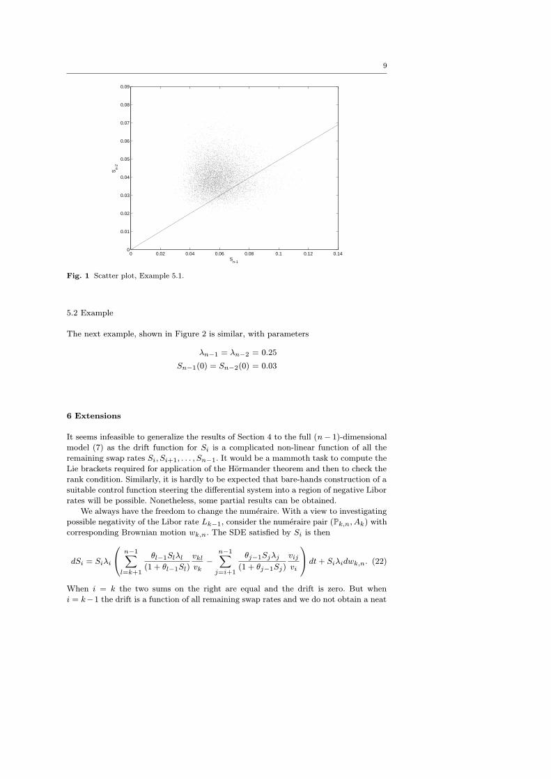
We performed a Monte Carlo simulation of 10000 paths of the system in (11) expressed
in Ito form with parameters
λn−1 = λn−2 = 0.2
Sn−1(0) = 0.05
Sn−2(0) = 0.04
Figure 1 is a scatter plot showing the 10000 sample values of Sn−1(T ) (horizontal
axis) and Sn−2(T ) (vertical axis) at T = 5 years. The line on the figure represents the
boundary in (16), namely
Sn−2 =Sn−1
a+ bSn−1.
The Libor rate Ln−2 is negative below this boundary, and we note that a significant
proportion of the paths arrive below the boundary.
9
0 0.02 0.04 0.06 0.08 0.1 0.12 0.140
0.01
0.02
0.03
0.04
0.05
0.06
0.07
0.08
0.09
Sn-1
Sn-
2
Fig. 1 Scatter plot, Example 5.1.
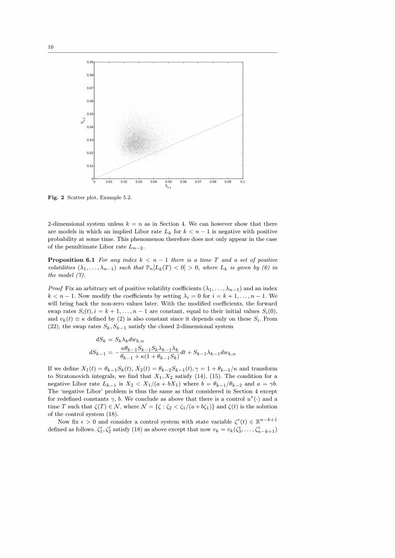
5.2 Example
The next example, shown in Figure 2 is similar, with parameters
λn−1 = λn−2 = 0.25
Sn−1(0) = Sn−2(0) = 0.03
6 Extensions
It seems infeasible to generalize the results of Section 4 to the full (n− 1)-dimensional
model (7) as the drift function for Si is a complicated non-linear function of all the
remaining swap rates Si, Si+1, . . . , Sn−1. It would be a mammoth task to compute the
Lie brackets required for application of the Hormander theorem and then to check the
rank condition. Similarly, it is hardly to be expected that bare-hands construction of a
suitable control function steering the differential system into a region of negative Libor
rates will be possible. Nonetheless, some partial results can be obtained.
We always have the freedom to change the numeraire. With a view to investigating
possible negativity of the Libor rate Lk−1, consider the numeraire pair (Pk,n, Ak) with
corresponding Brownian motion wk,n. The SDE satisfied by Si is then
dSi = Siλi
n−1∑
l=k+1
θl−1Slλl(1 + θl−1Sl)
vklvk−
n−1∑
j=i+1
θj−1Sjλj
(1 + θj−1Sj)
vij
vi
dt+ Siλidwk,n. (22)
When i = k the two sums on the right are equal and the drift is zero. But when
i = k−1 the drift is a function of all remaining swap rates and we do not obtain a neat
10
0 0.01 0.02 0.03 0.04 0.05 0.06 0.07 0.08 0.09 0.10
0.01
0.02
0.03
0.04
0.05
0.06
0.07
0.08
0.09
Sn-1
Sn-
2
Fig. 2 Scatter plot, Example 5.2.
2-dimensional system unless k = n as in Section 4. We can however show that there
are models in which an implied Libor rate Lk for k < n − 1 is negative with positive
probability at some time. This phenomenon therefore does not only appear in the case
of the penultimate Libor rate Ln−2.
Proposition 6.1 For any index k < n − 1 there is a time T and a set of positive
volatilities (λ1, . . . , λn−1) such that Pn[Lk(T ) < 0] > 0, where Lk is given by (6) in
the model (7).
Proof Fix an arbitrary set of positive volatility coefficients (λ1, . . . , λn−1) and an index
k < n − 1. Now modify the coefficients by setting λi = 0 for i = k + 1, . . . , n − 1. We
will bring back the non-zero values later. With the modified coefficients, the forward
swap rates Si(t), i = k + 1, . . . , n − 1 are constant, equal to their initial values Si(0),
and vk(t) ≡ κ defined by (2) is also constant since it depends only on these Si. From
(22), the swap rates Sk, Sk−1 satisfy the closed 2-dimensional system
dSk = Skλkdwk,n
dSk−1 = −κθk−1Sk−1Skλk−1λkθk−1 + κ(1 + θk−1Sk)
dt+ Sk−1λk−1dwk,n
If we define X1(t) = θk−1Sk(t), X2(t) = θk−2Sk−1(t), γ = 1 + θk−1/κ and transform
to Stratonovich integrals, we find that X1, X2 satisfy (14), (15). The condition for a
negative Libor rate Lk−1 is X2 < X1/(a + bX1) where b = θk−1/θk−2 and a = γb.
The ‘negative Libor’ problem is thus the same as that considered in Section 4 except
for redefined constants γ, b. We conclude as above that there is a control u∗(·) and a
time T such that ζ(T ) ∈ N , where N = ζ : ζ2 < ζ1/(a+ bζ1) and ζ(t) is the solution
of the control system (18).
Now fix ε > 0 and consider a control system with state variable ζε(t) ∈ Rn−k+1
defined as follows. ζε1, ζε2 satisfy (18) as above except that now vk = vk(ζε3, . . . , ζ
εn−k+1)
11
defined by (2) with Sk+i = ζε2+i/θk+i−1 (so (18) is no longer a closed system). The
remaining components ζε3, . . . , ζεn−k−1 satisfy the control system equations derived from
(22) with θl−1Sl ≡ ζεl−k+2 and λl replaced by ελl for l = k+1, . . . , n−1. In summary, we
are considering the closed system of swap rates Sk−1, . . . , Sn−1 but with all volatilities
λk+1, . . . , λn−1 scaled by a factor ε, and looking at the control system corresponding
to that.
A differential equation zε = f(t, ε, zε) in Rm with vector field f depending smoothly
on a parameter ε is equivalent to an ODE in Rm+1 defined by
zεi = fi(t, zεm+1, (z
ε1, . . . , z
εm)), i = 1 . . . ,m
zεm+1 = 0, zεm+1(0) = ε.
It follows from standard results about dependence of solutions of ODEs on the ini-
tial condition that for fixed T , limε→0 zε(T ) = z0(T ). Applying this to the above
control system with the fixed control u∗(·) determined above, we see that for any T ,
vk(ζε3(T ), . . . , ζεn−k+1(T )) → κ as ε → 0, while (ζε1(T ), ζε2(T )) → (ζ01 (T ), ζ0
2 (T )), the
solution of (18). Hence there exists ε′ > 0 such that ζε(T ) satisfies
ζε′
2 (T ) <ζε′
1 (T )
b(γε′
+ ζε′
1 (T ))
where γε′
= 1 + θk−1/vk(ζε′
3 (T ), . . .). This is the region in which the Libor rate Lk−1
is negative in the model with volatilities (λ1, . . . , λk, ε′λk+1, . . . , ε
′λn−1). Applying the
Support Theorem, we conclude that Pn[Lk−1(T ) < 0] > 0 in this model. ut
A further important question, which we do not explore here, is the dependence
of the support on the dimension d of the Brownian motion driving the swap market
model (7). The normal situation is that there are n = 10 or more swap rates but a much
smaller, say d = 2, 3 of Brownian motions, so we always have a degenerate system. It is
clear from the support theorem that the support can only increase if an extra Brownian
motion is added. The question is whether it is possible to have a model in which Libor
rates are positive up to some critical dimension d∗ but the support includes ‘negative
territory’ beyond that. We do not believe that this can be the case, but have no way
of proving it.
7 Concluding remarks
There are many outstanding questions in this research. We would certainly like to get a
more explicit characterization of the measures generated by swap market models that
goes beyond the 2-dimensional case solved by Jamshidian [6]. In particular, the key
question is the one discussed at the end of the preceding section: what is the effect of
the dimension of the Brownian motion on the support of the solution? It seems that
new techniques will be needed to answer this question.
Finally, we should say that it is not at all the present authors’ intention to caste
doubt on the value of the Swap Market Model as a practical tool. Practitioners are
certainly aware that there are sets of swap rates inconsistent with positive forward
Libor rates, and many will have no doubt observed occurrence of negative rates in
simulations, such as those presented in Section 5, where the initial rates are all positive.
But while these phenomena are familiar on an informal level, there has been very little

12
formal analysis, a situation we are seeking to rectify precisely because of the practical
importance of the model.
Acknowledgements We would like to thank Farshid Jamshidian for the interest he has takenin this work, and the referee and associate editor for their helpful comments and suggestions.
References
1. A. Brace, D. Gatarek and M. Musiela, The market model of interest rates, MathematicalFinance 7(2) (1997) 127-147
2. S. Galluccio, Z. Huang, J.-M. Ly and O. Scaillet, Theory and Calibration of Swap MarketModels, preprint 2004, to appear in Mathematical Finance
3. S. Galluccio and C. Hunter, The Co-initial Swap Market Model, Economic Notes by BancaMonte dei Paschi di Siena SpA 33(2) (2004) 209-232
4. N. Ikeda and S. Watanabe, Stochastic Differential Equations and Diffusion Processes,North Holland-Kodansha, Amsterdam and Tokyo 1981
5. F. Jamshidian, Libor and swap market models and measures, Finance & Stochastics 7(1997) 293-300
6. F. Jamshidian, Bivariate support of forward Libor and swap rates, Working paper, NIB-Capital Bank and University of Twente, Netherlands 2006
7. K. Miltersen, K. Sandmann and D. Sondermann, Closed form solutions for term structurederivatives with log-normal interest rates, The Journal of Finance 52(2) (1997) 409-430
8. M. Musiela and M. Rutkowski, Continuous-time term structure models: Forward measureapproach Finance and Stochastics 1 (1997) 261-291
9. L.C.G. Rogers and D. Williams, Diffusions, Markov Processes and Martingales, vol. 2,Cambridge University Press 2000
10. D.W. Stroock and S.R.S. Varadhan, On the support of diffusion processes with applicationsto the strong maximum principle, Proc. 6th Berkeley Symp. Math. Statist. Prob. 3 (1972)333-359


