
NBER WORKING PAPER SERIES
GLOBALIZATION AND DIRTY INDUSTRIES:DO POLLUTION HAVENS MATTER?
Jean-Marie GretherJaime de Melo
Working Paper 9776http://www.nber.org/papers/w9776
NATIONAL BUREAU OF ECONOMIC RESEARCH1050 Massachusetts Avenue
Cambridge, MA 02138June 2003
Chapter forthcoming in “Challenges ot Globalization”. An earlier version of this paper was presented at theCEPR/NBER/SNS International Seminar on International Trade "Challenges to Globalization", Stockholm,24/25 May 2002. We thank Céline Carrère for data and much appreciated support, Nicole Mathys forexcellent research assistance, Robert Baldwin for many helpful suggestions, and conference participants foruseful comments. The views expressed herein are those of the authors and not necessarily those of theNational Bureau of Economic Research.
©2003 by Jean-Marie Grether and Jaime de Melo. All rights reserved. Short sections of text not to exceedtwo paragraphs, may be quoted without explicit permission provided that full credit including © notice, isgiven to the source.

Globalization and Dirty Industries: Do Pollution Havens Matter?Jean-Marie Grether and Jaime de MeloNBER Working Paper No. 9776June 2003JEL No. F18, Q28
ABSTRACT
This paper reviews arguments and evidence on the impact of globalization on the environment, then
presents evidence on production and international trade flows in five heavily polluting industries for
52 countries over the period 1981-98. A new decomposition of revealed comparative advantage
(RCA) according to geographical origin reveals a delocalization to the South for all heavily polluting
industries except non-ferrous metals that exhibits South-North delocalization in accordance with
factor-abundance driven response to a reduction in trade barriers. Panel estimation of a gravity
model of bilateral trade on the same data set reveals that, on average, polluting industries have
higher barriers-to-trade costs (except non-ferrous metals with significantly lower barriers to trade)
and little evidence of delocalization in response to a North-South regulatory gap.
Jean-Marie Grether Jaime de MeloGroupe d’économie politique Département d’économie politique 7 Rue Pierre-à-Mazel 40, boulevard du Pont-d’ArveUniversité de Neuchâtel Université de GenèveCH-2000 Neuchâtel CH-1211 Genève 4Siwtzerland [email protected] [email protected]
2
1 Introduction
In the debate on globalization and the environment, there is
concern that the erasing of national borders through reduced
barriers to trade will lead to competition for investment and
jobs, resulting in a worldwide degradation of environmental
standards (the `race to the bottom´ effect) and /or in a
delocalization of heavy polluting industries in countries with
lower standards (the `pollution havens´ effect). Moreover,
environmentalists and ecologically-oriented academics argue
that the political economy of decision-making is stacked up
against the environment. In the North, OECD interest groups
that support protectionist measures for other reasons continue
to invoke the race-to-the-bottom model, relying on the
perception that the regulatory gap automatically implies a race
to the bottom, even though some have argued that countries may
circumvent international agreements on tariffs by choosing
strategic levels of domestic regulation. Because avoidance of a
race to the bottom would call for the enforcement of uniform
environmental standards in all countries, which cannot be
created, they argue for trade restrictions until the regulatory
gap is closed. In the South, corruption is likely to result in
poor enforcement of the regulatory framework. Finally, at the
international level, environmental activists fear that the
dispute settlement mechanism of the WTO favors trade interests
over environmental protection.
To sum up, the arguments raised above, as well as empirical
evidence reviewed below, suggest that trade liberalization and
globalization (in the form of reduced transaction costs) could
lead to a global increase in environmental pollution as well as
to an increase in resource depletion as natural resource
exploiting industries, from forest logging companies to mining,
3
relocate to places with less strict standards or use the threat
of relocation to prevent the imposition of stricter standards.
These effects are likely to be more important the further is
environmental policy from the optimum and the less well-defined
are property rights as is the case for the so-called ‘global
commons’. It is therefore not surprising that, even if trade
liberalization and globalization more generally can lead to
both an overall increase in welfare (especially if
environmental policy is not too far from the optimum) and to a
deterioration in environmental quality, a fundamental clash
will persist between free trade proponents and
environmentalists.
This paper addresses the relation between globalization and the
environment by re-examining evidence of a North-South
delocalization of heavily polluting industries.1 Section 2
reviews the evidence on `pollution havens´2, arguing that it is
either too detailed (firm-specific of emission-specific
evidence) or too fragmentary (case studies) to give a broad
appreciation of the extent of delocalization over the past
twenty years. The following sections then turn to new evidence
based on 3-digit ISIC production and trade data for 52
countries over the period 1981-98.3 In section 3, we report on
the worldwide evolution of heavy polluters (the so-called
`dirty‘ industries) and on the evolution of North-South
revealed comparative advantage indexes. Section 4 then
estimates a panel gravity trade model to examine patterns of
trade in polluting products. Estimates reveal that transport
1 The causes of any detected relocation will not be identified because weare dealing with fairly aggregate data.2 In the public debate, the ‘pollution havens’ effect refers either to anoutput reduction of polluting industries (and an increase in imports) indeveloped countries or to the relocation of industries abroad via FDI inresponse to a reduction in import protection or a regulatory gap.3 The main data base has been elaborated by Nicita and Olarreaga (2001). Anappendix to the paper describes data manipulation and the representativityof the sample in terms of global trade and production in pollutingactivities.
4
costs may have acted as a brake on North-South relocation, and
fail to detect a regulatory gap effect.
2. Pollution Havens or pollution Halos?
We review first the evidence on trade liberalization and
patterns of trade in polluting industries based on multi-
country studies that try to detect evidence of North-South
delocalization. We then summarize results from single-country,
often firm-level, studies that use more reliable environmental
variables and are also generally better able to control for
unobservable heterogeneity bias. We conclude with lessons from
case studies and political-economy considerations.
2.1 Evidence on production and trade in dirty products
Evidence from aggregate production and trade data is based on a
comparison between ‘clean’ and ‘dirty’ industries, the
classification relying invariably on U.S. data, either on
expenditure abatement costs, or on emissions of pollutants.4
Table 1 summarizes the results from these studies. Overall, the
studies, which for the most part use the same definition of
dirty industries as we do5, usually find mild support for the
pollution havens hypothesis.
4 Most work on the US is based on pollution abatement capital expendituresor on pollution abatement costs (See e.g. Levinson and Taylor (2002, table1). It turns out that the alternative classification based on emissions(see Hettige et al. 1995) produces a similar ranking for the cleanest anddirtiest industries (5 of the top 6 pollution industries are the same inboth classifications).5 As in this paper, polluting industries were classified on the basis ofthe comprehensive index of emissions per unit of output described inHettige et al. (1995). That index includes conventional air, water andheavy metals pollutants. As to the applicability of that index based on USdata to developing countries, Hettige et al. conclude (p. 2) that, eventhough pollution intensity is likely to be higher, “the pattern of sectoralrankings may be similar”.
5
Insert table 1 here:
Multi-country papers on trade and environmental costs
The large number of countries and the industrial-level approach
gives breadth of scope to the studies described in table 1, but
at a cost. First changing patterns of production and trade
could be due to omitted variables and unobserved heterogeneity
that cannot be easily controlled for in large samples where
aggregated data say very little about industry choices which
would shed light on firms or production stages (Zarsky (1999,p
66)). For example, as pointed out by Mani and Wheeler in their
case study of Japan, changes in local factor costs (price of
energy, price of land) and changes in policies other than the
stringency of environmental regulations could account for
observed changes in trade patterns. Second, these studies give
no evidence on investment patterns, and how these might react
to changes in environmental regulation, which is at the heart
of the ‘pollution havens’ debate.6 It is therefore not totally
surprising that the papers surveyed in Dean (1992) and Zarsky
(1999), by and large, fail to detect a significant correlation
between the location decision of multinationals and the
environmental standards of host countries. This suggests that,
after all, when one goes beyond aggregate industry data, the
“pollution havens” hypothesis may be a popular myth.
Recent studies respond to the criticism that the evidence so
far does not address the research needs because of excessive
6 Smarzynska and Wei (2001) cite the following extract from "A Fair TradeBill of Rights" proposed by the Sierra Club: “in our global economy,corporations move operations freely around the world, escaping toughcontrol laws, labor standards, and even the taxes that pay for social andenvironmental needs”.
6
aggregation. However, this recent evidence, summarized below,
is still very partial, and heavily focussed on the US.
2.2 Evidence on the location of dirty industries
Levinson and Taylor (2002) revisit the single-equation model of
Grossman-Krueger (1993) using panel data for US imports in a
two-equation model in which abatement costs are a function of
exogenous industry characteristics while imports are a function
of abatement costs. Contrary to previous estimates, they find
support for the pollution havens hypothesis: industries whose
abatement costs increased the most, saw the largest relative
increase in imports from Mexico, Canada, Latin American and the
rest-of-the-world. 7
Drawing on environmental costs across the US that are more
comparable than the rough indices that must be used in cross-
country work, Keller and Levinson (2001) analyze inward FDI
into the US over the period 1977-94. They find robust evidence
that relative (across States) abatement costs had moderate
deterrent effects on foreign investment.
Others have analyzed outward FDI to developing countries.
Eskeland and Harrison (2002), examine inward FDI in Mexico,
Morocco, Venezuela and Côte d’Ivoire at the four-digit level
using US abatement cost data controlling for country-specific
factors. They find weak evidence of some FDI being attracted to
sectors with high levels of air pollution, but no evidence of
FDI to avoid abatement costs. They also find that foreign firms
are more fuel-efficient in that they use less ‘dirty fuels’.
7 Ederington and Minier (2001) also revisit the Grossman-Krueger study,assuming that pollution regulation is also endogenous, but determined bypolitical-economy motives. They also find support for the pollution-havens
7
This evidence supports the ‘pollution halo’ hypothesis:
superior technology and management, coupled with demands by
“green” consumers in the OECD, lift industry standards
overall.8
Smarzynska and Wei (2001), estimate a probit of FDI of 534
multinationals in 24 transition economies during the period
1989-94 as a function of host country characteristics. These
include a transformed (to avoid outlier dominance) US-based
index of dirtiness of the firm at the 4-digit level, an index
of the laxity of host country’s environmental standards
captured by a corruption index, and several measures of
environmental standards (participation in international
treaties, quality of air and water standards, observed
reductions in various pollutants). In spite of this careful
attempt at unveiling a ‘pollution haven’ effect, they conclude
that host-country environmental standards (after controlling
for other country characteristics including corruption) had
very little impact on FDI inflows.
2.3 Case studies and political-economy considerations
Reviewing recently available data, Wheeler (2000) shows that
suspended particulate matter release (the most dangerous form
of air pollution) has been declining rapidly in Brazil, China,
Mexico, fast growing countries in the era of globalization and
big recipients of FDI. Organic water pollution is also found to
fall drastically as income per capita rises (poorest countries
have approximately tenfold differential pollution intensity).9
hypothesis, this time because inefficient industries seek protection viaenvironmental legislation.8 The mixed evidence on the pollution halo hypothesis is reviewed in Zarsky(1999).9 These results accord with independent estimates of environmentalperformance constructed by Dasgupta et al. (1996) from a responses to a
8
In addition to the standard explanations (pollution control is
not a critical cost factor for firms, large multinationals
adhere to OECD standards), he also points out that case studies
show that low-income communities often penalize dangerous
polluters even when formal regulation is absent or weak.
Wheeler concludes that the “bottom” rises with economic growth.
This result is reinforced by recent evidence based on a
political-economy approach that endogenizes corruption in the
decision-making process. Assuming that governments’ accept
bribes in formulation of their regulatory policies, Damia et al
(2000) find support in panel data for 30 countries over the
period 1982-92 that the level of environmental stringency is
negatively correlated with an index of corruption and
positively with an index of trade openness. Given that
corruption is typically higher in low-income countries, this
corroborates the earlier finding mentioned above, that
environmental stringency increases rapidly with income.
3. Shifting patterns of production and comparative advantage
in polluting industries
Direct approaches to the measurement of pollution emission
(e.g. Grossman and Krueger (1995), Dean (2000), Antweiler,
Copeland and Taylor (2001) and several of the studies mentioned
above) use emission estimates at geographical sites of
pollutant particles (sulfur dioxide is a favorite) or the
release of pollutants in several media (air, water, etc…). That
approach has several advantages: emissions are directly
measured at each site, and it is not assumed that pollutant
intensity is the same across countries. On the other hand
detailed questionnaire administered to 145 countries (they find acorrelation of about 0.8 between their measure of environment performance
9
activity (e.g. production levels) is not measured directly.
Arguably, this is a shortcoming if one is interested in the
pollution haven hypothesis. Indeed, emissions could be high for
other reasons than the relocation of firms to countries with
low standards (China’s use of coal as an energy source is
largely independent of the existence of pollution havens).
The alternative chosen here is to use an approach in which
emission intensity is not measured directly. We adopt the
approach in the studies summarized in table 1 where dirty
industries are classified according to an index of emission
intensity in the air, water and heavy metals in the US
described in footnote 4. We selected the same five most
polluting industries in the US in (1987) selected by Mani and
Wheeler (1999) (three-digit ISIC code in parenthesis): Iron and
Steel (371); Non-ferrous metals (372); Industrial chemicals
(351); Non-metallic mineral products (369); pulp and paper
(341).10 According to Mani and Wheeler (1998), compared to the
five cleanest U.S. manufacturing activities (textiles (ISIC
321), Non-electric machinery (382), Electric machinery (383),
transport equipment (384), instruments (385), the dirtiest have
the following characteristics: 40% less labor-intensive;
capital-output ratio twice as high; and an energy-intensity
ratio three times as high.
3.1 Shifting patterns of production
We start with examination of the broad data for our sample of
52 countries over the period 1981-98. The sample (years and
countries) is the largest for which we could obtain production
data matching trade data at the 3-digit ISIC level. Compared to
or environment policy and income per capita).
10
the earlier studies mentioned in table 1, this sample has
production data for a larger group of countries, though at a
cost because comprehensive data--only available since 1981--
implies that we are missing some of the early years of
environmental regulation in OECD countries in the seventies.
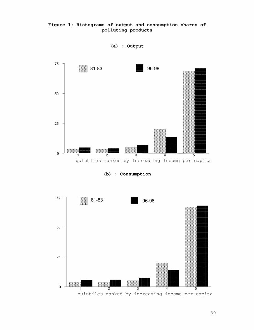
Because there is a close correlation between the stringency of
environmental regulation and income per capita, we start with
histograms of indices of pollution intensity ranked by income
per capita quintile (the data are three-year averages at the
beginning and end of period). Given our sample size, each
quintile has 10 or 11 observations.
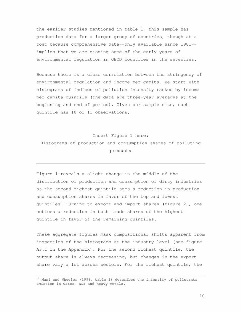
Insert Figure 1 here:
Histograms of production and consumption shares of polluting
products
Figure 1 reveals a slight change in the middle of the
distribution of production and consumption of dirty industries
as the second richest quintile sees a reduction in production
and consumption shares in favor of the top and lowest
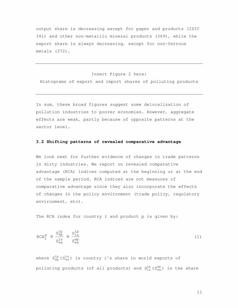
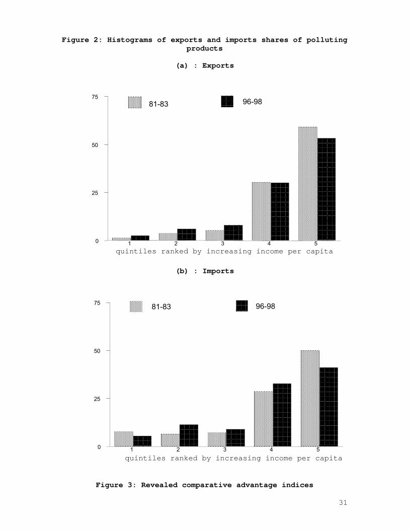
quintiles. Turning to export and import shares (figure 2), one
notices a reduction in both trade shares of the highest
quintile in favor of the remaining quintiles.
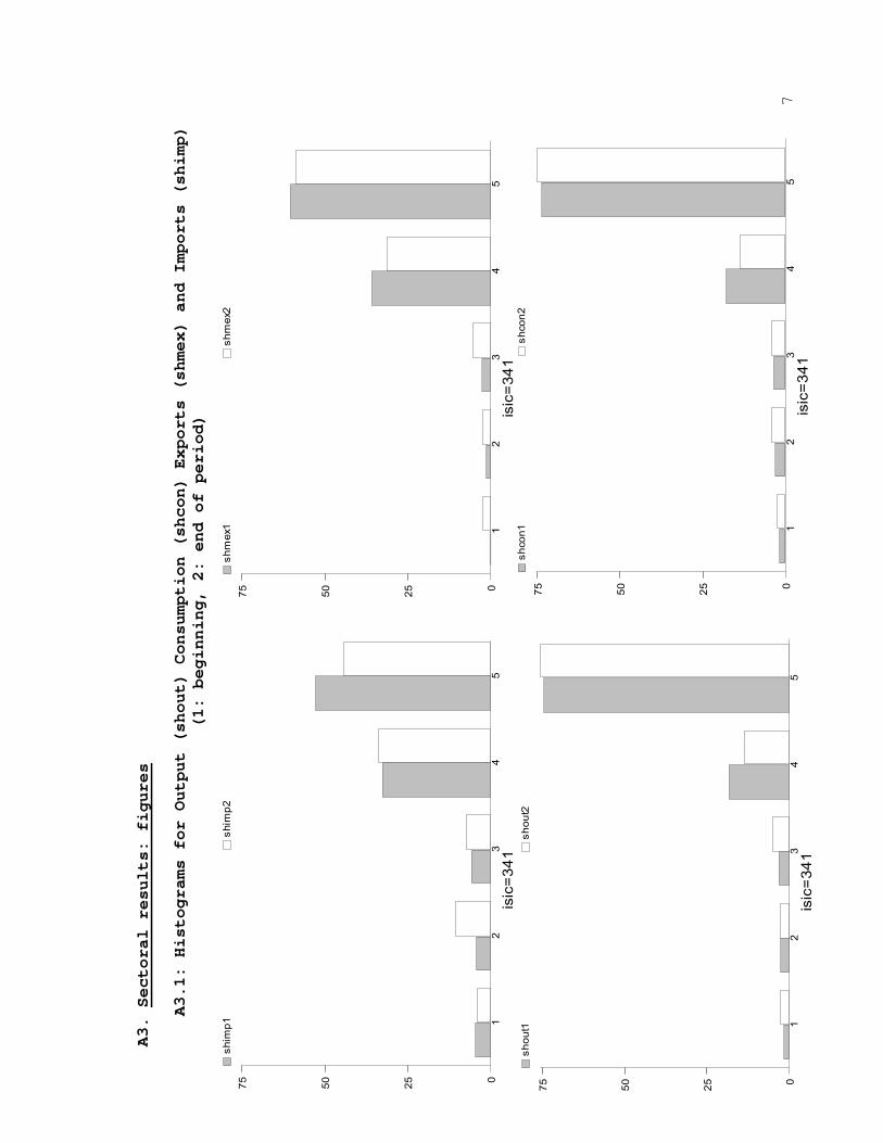
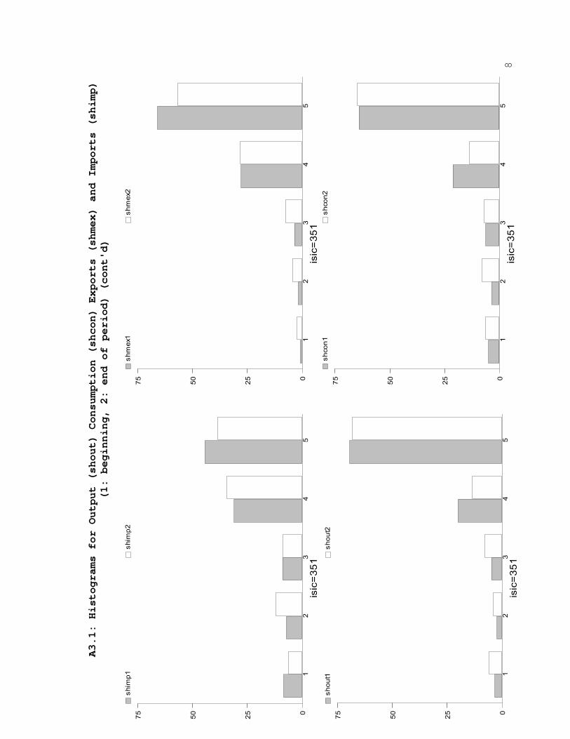
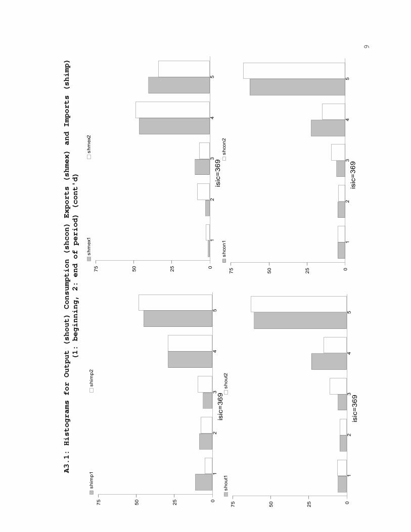
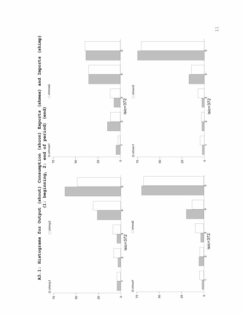
These aggregate figures mask compositional shifts apparent from
inspection of the histograms at the industry level (see figure
A3.1 in the Appendix). For the second richest quintile, the
output share is always decreasing, but changes in the export
share vary a lot across sectors. For the richest quintile, the
10 Mani and Wheeler (1999, table 1) describes the intensity of pollutantsemission in water, air and heavy metals.
11
output share is decreasing except for paper and products (ISIC
341) and other non-metallic mineral products (369), while the
export share is always decreasing, except for non-ferrous
metals (372).
Insert Figure 2 here:
Histograms of export and import shares of polluting products
In sum, these broad figures suggest some delocalization of
pollution industries to poorer economies. However, aggregate
effects are weak, partly because of opposite patterns at the
sector level.
3.2 Shifting patterns of revealed comparative advantage
We look next for further evidence of changes in trade patterns
in dirty industries. We report on revealed comparative
advantage (RCA) indices computed at the beginning or at the end
of the sample period. RCA indices are not measures of
comparative advantage since they also incorporate the effects
of changes in the policy environment (trade policy, regulatory
environment, etc).
The RCA index for country i and product p is given by:
wpwa
ipia
iawa
ipwpp
iS
S
S
SRCA == (1)
where ipwpS ( ia
waS ) is country i’s share in world exports of
polluting products (of all products) and ipiaS ( wp
waS ) is the share
12
of polluting products in total exports of country i (of the
world).
Countries are split into two income groups (see table A1 in the
Appendix) that replicate the distinction between the three
poorest and two richest quintiles of the previous section: 22
high income countries (1991 GNP per capita larger than 7910 USD
according to the World Bank) and 30 low and middle-income
countries. Hereafter the former group is designed by developed
countries (DCs) or "North", the latter by less developed
countries (LDCs) or "South".
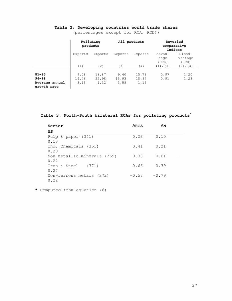
A first glimpse at the aggregate figures (see table 2) confirms
that LDCs’ share in world trade of polluting products is on the
rise. But the average annual rate of growth is lower for
polluting products than for exports in general. As a result,
LDCs as a whole exhibit a decreasing RCA (and an increasing
revealed comparative disadvantage) in polluting products (see
last columns of table 2).
Insert table 2 here:
Share of developing countries in world trade
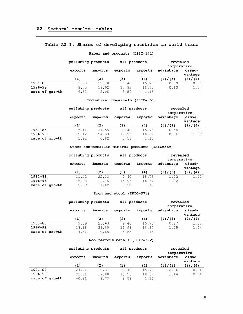
However, inspection at the industry level (see table A2.1,
reveals that this reverse-delocalization outcome is due to the
dominating effect of non-ferrous metals (ISIC 372). All other
four industries present some ingredient of delocalization, with
a particularly strong increase in RCA for industrial chemicals
(351). Interestingly, non-ferrous metals represented more than
40% of LDCs exports at the beginning and less than 25% at the
end of the period, while the pattern is exactly opposite for
industrial chemicals.
13
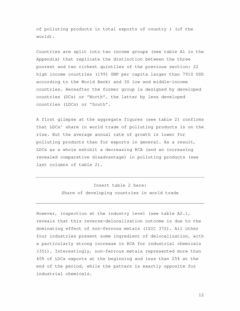
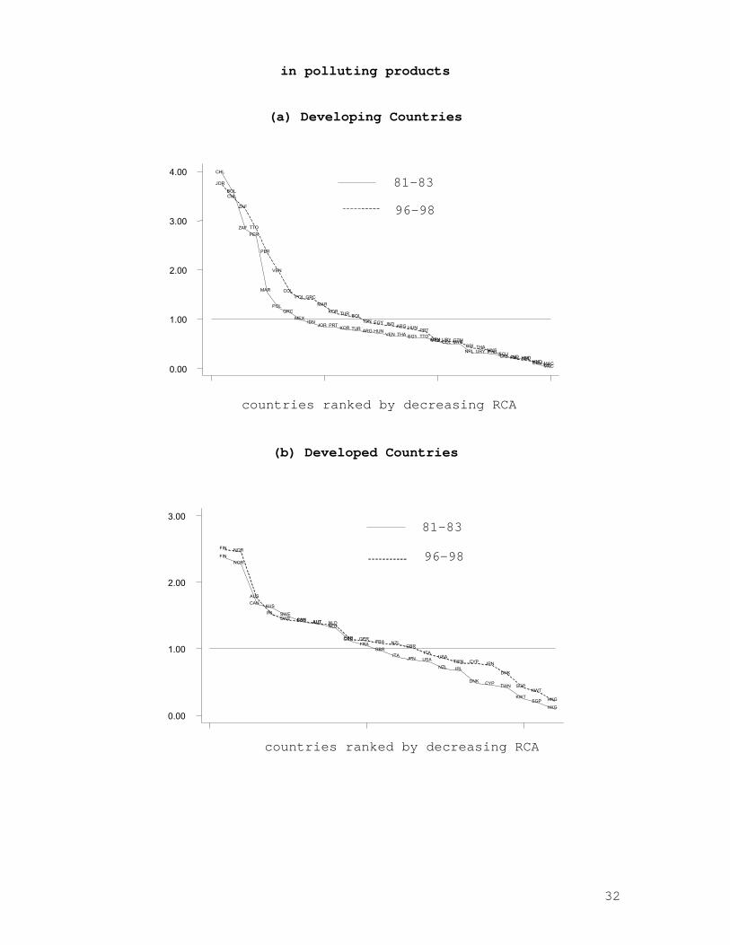
To unveil cross-country variations, figure 3 ranks countries by
decreasing order of RCAs for both income groups. In each case,
the dashed line represents the end-of-period pattern with
countries ranked by decreasing order of comparative advantage
so that all observations above (below) unity correspond to
countries with a a revealed comparative advantage
(disadvantage). A shift to the right (left) implies increasing
(decreasing) revealed comparative advantage, and a flattening
of the curve, a less pronounced pattern of specialization.
Figure 3:
Revealed comparative advantage indices in polluting products
Overall, LDCs’ pattern of RCAs is characterized by higher upper
values of RCAs and a steeper curve than high-income countries.
Over time, both curves appear to shift right11 and become
somewhat flatter. The increase in RCAs seems larger in LDCs,
where it is concentrated in the middle of the distribution,
while it basically affects the end of the distribution in the
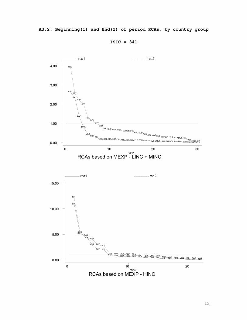
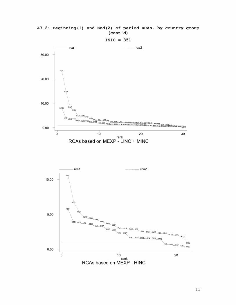
other income group. At the industry level (see figure A3.2)
results for LDCs are quite similar, expect for non-ferrous
metals, where the RCA curve shifts in12.
Still, the above pattern does not say anything about the
changing pattern of RCAs between the North and the South, which
is what the delocalization hypothesis is about. To measure this
11 This result may seem puzzling but the contradiction is only apparent: theweighted sum of RCAs is indeed equal to 1.0, but the weights can vary.Thus, a simultaneous increase in all RCA indices may well happen, provideda larger weight is put on smaller values.
12 Note that the pattern illustrated by figure 3 only reflects a"structural" effect, i.e. the change of individual RCAs. The evolution ofthe aggregate RCA for LDCs as a group is also governed by a "composition"effect, namely the impact of changes in countries' shares keeping RCAindices constant. Straightforward calculations reveal that for LDCs thecomposition effect (-0.19) has been stronger than the structural effect(0.13), leading to a net decrease of the aggregate RCA reported in table 2(for results at the industry level, see table A2.2).
14
effect, we introduce a new decomposition that isolates the
impact of geography on the RCA index. From (1), note that the
RCA of country i in product p ( piRCA ) can be decomposed into:
∑=
=N
1j
ijaiwa
pij
pi SRCARCA (2)
where the bilateral RCA ( pijRCA ) is defined as the ratio between
the share of product p in all exports of country i to country j
( ijpijaS ) and the share of product p in total world exports ( wp
waS ).
This share is weighted by the share of country j in total
exports country i to the world ( ijaiwaS ).
Now let the world be divided in two groups of countries: nS in
the South, nN in the North (nS+nN=N). Then (2) can be rewritten:
∑∑==
+≡+=NS n
1j
ijaiwa
pij
n
1j
ijaiwa
pij
pi
pi
pi SRCASRCANSRCA (3)
where piS is the South's contribution and p
iN the North's
contribution to piRCA . Thus, in terms of variation between the
end (96-98) and the beginning (81-83) of the sample period, one
obtains:
pi
pi
pi NSRCA ∆+∆=∆ (4)
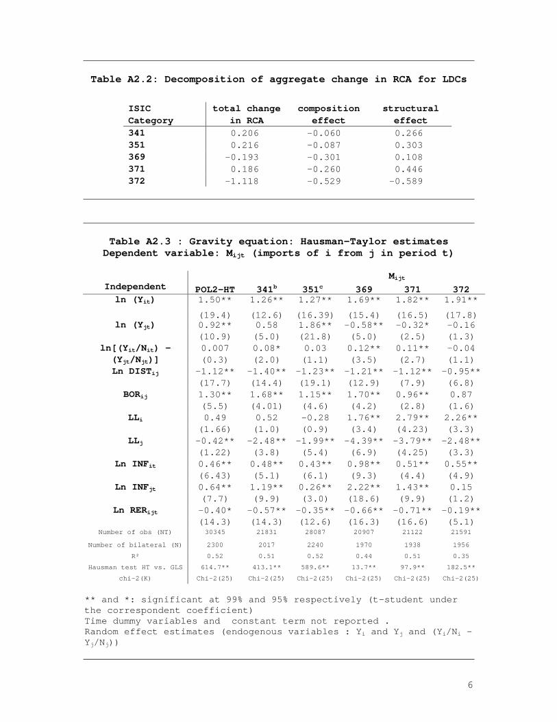
Results from applying this decomposition to the two groups of
countries are reported in table 3. For each polluting sector,
we report the (unweighted) average of both sides of equation
15
(4) over the LDCs’ group. It appears that in all cases but one,
the North's contribution to the change in LDCs’ RCA is
positive. This result is consistent with the pollution haven
effect. Again, the only exception is non-ferrous metal, where
North-South trade has negatively contributed to the RCA of the
South.
Insert table 3 here:
Table 3: North-South bilateral RCAs for polluting products
In sum, the RCA-based evidence on delocalization of polluting
activities towards the South is rather mixed. As a group,
developing countries exhibit a surprising reverse-
delocalization pattern of increasing revealed comparative
disadvantage in polluting products. However, as shown above,
this reflects both the pattern of one particular industry (non-
ferrous metals) and a composition effect: within the group of
developing countries, those less prone to export polluting
products have gained ground. In fact, most developing countries
have in fact experienced an increase in their RCA in polluting
products. Moreover, after controlling for geography, it turns
out that for all but for one case (non-ferrous metals), North-
South trade has had a positive impact on LDCs' comparative
advantage in these products.
4. Bilateral trade patterns in polluting products
Dirty industries are typically weight-reducing industries. They
are also intermediate-goods producing industries. As a result
if they move to the South, then transport costs must be
incurred if the final (consumer goods) products are still
produced in the North, as would be the case, for example in the

16
newspaper printing industry. Hence the reduction in transport
costs and protection that has occurred with globalization may
not have had much effect on the location of these industries.
Our third piece of evidence consists of checking if, indeed,
polluting industries are not likely to relocate so easily
because of relatively high transport costs. To check whether
this may be the case, we estimate a standard bilateral trade
gravity model for polluting products, and compare the
coefficients with those obtained for non-polluting
manufactures.
Take the simplest justification for the gravity model: trade is
balanced (in this case at the industry level which some would
find unrealistic), and each country consumes its output, and
that of other countries according to its share, si, in world
GNP, YW. Then (see Rauch, 1999), bilateral trade between i and
j will be given by: Mij= (2YiYj)/YW = f(Wij). The standard
“generalized” gravity equation (which can be obtained from a
variety of theories) can be written as: Mij= f(Wij)(θij)-σ where
θij is an index of barriers-to-trade between i and j, Wij is a
vector of other intervening variables that includes the
bilateral exchange rate, eij, and prices, and σ is an estimate
of the ease of substitution across suppliers.
In the standard estimation of the gravity model, θij is
captured either by distance between partners, or if one is
careful, by relative distance to an average distance among
partners in the sample, DIST, i.e. by, DTij=DISTij/DIST. Dummy
variables that control for characteristics that are specific to
bilateral trade between i and j (e.g. a common border, BORij,
landlockedness in either country, LLi (LLj)) are also
17
introduced to capture the effects of barriers to trade.13 Here,
we go beyond the standard formulation by also including an
index of the quality of infrastructure in each country in
period t, INFit (INFjt), higher values of the index
corresponding to better quality of infrastructure.14 Finally,
because we estimate the model in panel, we include the
bilateral exchange rate, RERijt, defined so that an increase in
its value implies a real depreciation of i’s currency.
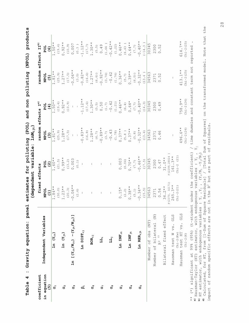
The above considerations lead us to estimate in panel the
following model (expected signs in parenthesis):
lnMijt = α0 + αt + αij + α1lnYit + α2lnYjt + α3lnINFit +
α4lnINFjt + α5lnRERijt + α6BORij + α7LLi + α8LLj + (5)
[α9lnDYijt] + β1lnDTij + ηijt
(α1>0, α2>0, α3>0, α4>0, α5<0 α6>0, α7<0, α8<0, β1<0)
In (5), α0 is an effect common to all years and pairs of
countries (constant term), αt an effect specific to year t but
common to all countries (e.g. changes in the price of oil), αij
an effect specific to each pair of countries but common to all
years and ηijt is the error term.
In a second specification we introduce the difference in GNP
per capita DYij = [(Yi/Ni)-(Yj/Nj)] in the equation, this
additional variable presumably capturing the effects of the
13 Brun et al. (2002) argue that the standard barriers-to-trade function ismispecified and propose a more general formulation that captures bothvariables that include country-specific characteristics, and variables thatcapture time-dependent costs (e.g. the price of oil). Since here we areonly interested in country-specific characteristics, time-dependent shocksare captured by time dummies.14 The index is itself a weighted sum of four indices computed each year:road density, paved roads, railway and the number of telephone lines percapita.
18
regulatory gap across countries. If the regulatory gap effect
is important, one would expect a positive sign for α9.15
For estimation purposes, equation (5) can be rewritten as:
lnMijt= Xijtϕ + Zijδ+ uijt with uijt = µij + νijt (6)
where X (Z) represents the vector of variables that vary over
time (are time-invariant) and a random error-component is used
because the within-transformation in a fixed-effects model
removes the variables that are cross-sectional time invariant.
To deal with the possibility of correlation between the
explanatory variables and the specific effects, we use the
instrument variable estimator proposed by Hausman and Taylor
(1981). However, we also report fixed-effects estimates which
correspond to the correct specification under the maintained
hypothesis (columns 1 & 2 of table 4).
Because the null hypothesis of correlation between explanatory
variables and the error term cannot be rejected, we re-
estimated the random-effects model treating the GDP variables
as endogenous. The results are reported in columns 3-6 of table
4. Coefficient estimates are robust and, after instrumentation,
the coefficient estimates are quite close in value to those
obtained under the fixed-effects estimates.
Insert table 4 here:
Gravity model: panel estimates
First note that all coefficients have the expected signs and,
as usual in gravity models with large samples, are robust to
15 In a full-fledged model with endogenous determination of environmentalpolicy, Antweiler et al. (2001) obtain a reduced form in which thetechnique effect (change in environmental policy) is captured by changes inincome per capita.

19
changes in specification.16 Notably, the dummy variables for
infrastructure have the expected signs and are highly
significant. So is the real exchange rate variable which
captures, at least partly, some of the effects of trade
liberalization that would not have already been captured in the
time dummy variables (not reported here). Income variables are
also, as expected, highly significant. Overall then, except for
the landlocked variables, which are at times insignificant, all
coefficient estimates have expected signs and plausible values.
Compare now the results between the panel estimates for all
manufactures --except polluting products—(column 5) with those
for the five polluting industries (column 6). Note first that
the estimated coefficient for distance is a third higher for
the group of polluting industries compared to the rest of
manufacturing.17 Second, note that the proxy for the regulatory
gap captured by the log difference of per capita GNPs is
negative for non-polluting manufactures (as one would expect
from the trade theory literature under imperfect competition
where trade flows are an increasing function of the similarity
in income per capita) while it is insignificant (though
positive) for polluting industries. Now, if indeed the
regulatory gap can be approximated by differences in per capita
GDPs across partners, the presence of pollution havens would be
reflected in a significant positive coefficient for this
variable.
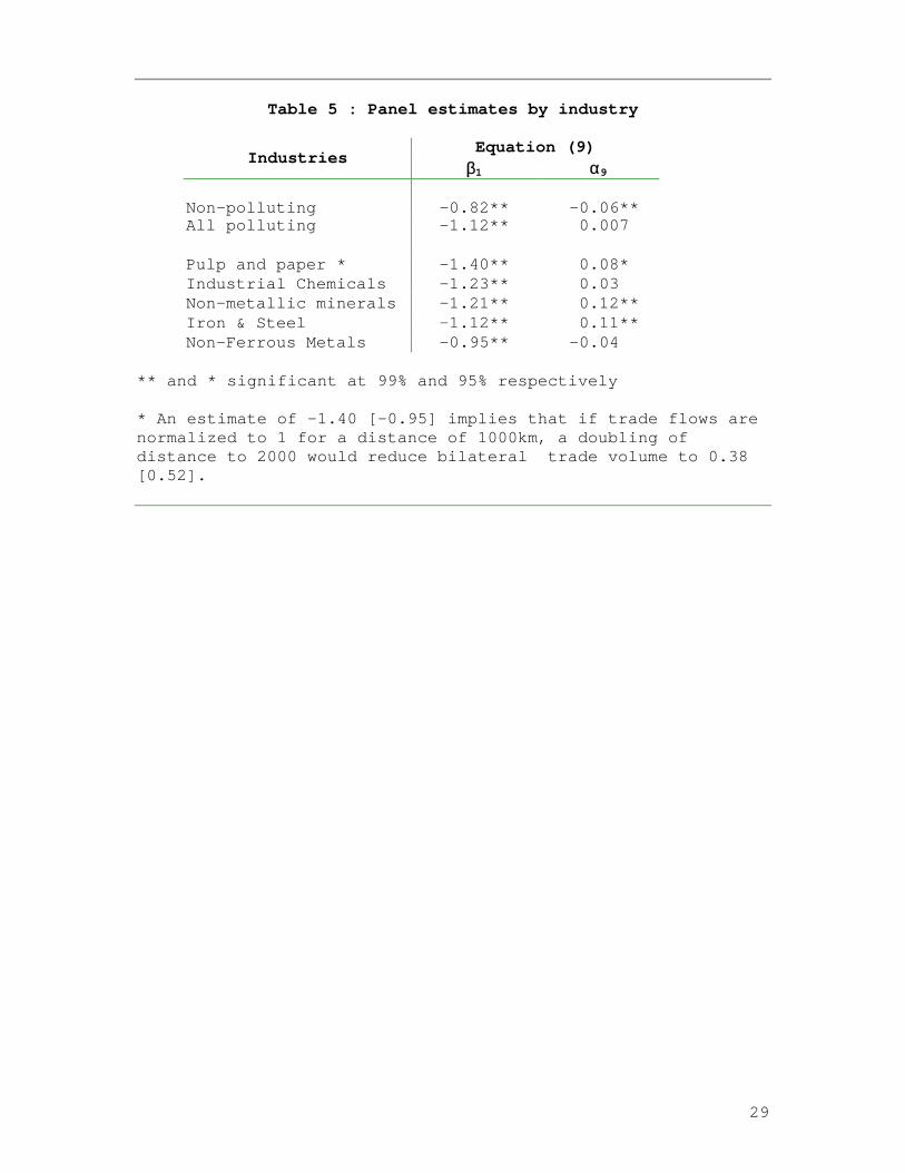
Compositional effects for the coefficients of interest are
shown in table 5. Non-ferrous metals (and to a lesser extent
iron & steel) stand out with low elasticity estimates for
16We also experimented with other variants (not reported here) by includingpopulation variables and obtained virtually identical estimates for theincluded variables.

20
distance. If one were to take seriously cross-sector
differences in magnitude, one would argue that the South-North
‘reverse’ (in the sense of the pollution havens hypothesis)
delocalization of non-ferrous metals according to comparative
advantage in response to the reduction in protection would have
occurred because of fewer natural barriers to trade. Of course,
there are other factors as well to explain the developments in
these sectors, including the heavy protection of these
industries in the North.
Insert table 5 here:
Panel estimates by industry
The sectoral pattern of estimates for α9 indicates that the
regulatory gap would have had an effect on bilateral trade
patterns for two sectors: non-metallic minerals and iron &
steel, and marginally for the pulp & paper industry. Again, the
non-ferrous metals stands out, suggesting no effect of
differences in the regulatory environment, once other
intervening factors are controlled for.
In sum, the pattern of trade elasticities to transport costs
obtained here makes sense. Most heavy polluting sectors are
intermediate goods, so proximity to users should enter into
location decisions more heavily than customs goods that are
typically high-value, low-weight industries that can be shipped
by airfreight. Interestingly, after controlling for a number of
factors that influence the volume of bilateral trade, we find
little evidence of the presence of a regulatory gap, thus
broadly supporting (indirectly) the ‘pollution halo’
hypothesis.
17 One could note that the coefficient estimates on infrastructure are muchhigher for these weight reducing activities which is also a plausible
21
5. Conclusions
Concerns that polluting industries would ‘go South’ was first
raised in the late eighties at the time when labor intensive
activities like the garment industries were moving South in
response to falling barriers to trade worldwide. Such
delocalization could be characterized as a continuous search
for ‘low-wage havens’ by apparel manufacturers in an industry
that has remained labor-intensive. Fears about pollution havens
were already expressed at the time notably because of the
possible impact of the regulatory gap between OECD economies
where polluters paying more would lead them to search for
‘pollution havens’ analogous to ‘low-wage havens’. Later with
the globalization debate, the hypothesis gained new momentum by
those who have read into globalization a breakdown of national
borders, making it difficult to control location choices by
multinationals.
This paper started with a review of the now substantial
evidence surrounding this debate which can be classified in
three rather distinct families. First, aggregate comparisons of
output and trade trends based on a classification of pollution
industries based on US emissions revealed very marginal
delocalization to the South. Second, firm-level estimates of
FDI location choices by-and-large found at best marginal
evidence either of location choice in the US in response to
cross-State differences in environmental regulations, or of
location choices by multinational firms across developing
countries in response to differences in environmental
regulations. Reasons for this lack of response to the so-called
regulatory gap were found in the third piece of evidence
largely assembled from developing-country case studies. Taking
into account political economy determinants of multinational
result signifying another brake on North-South delocalization.

22
behavior in host countries and the internal trade-offs between
leveling up emission standards (to avoid dealing with multiple
technologies) and cutting abatement expenditures, overall this
literature finds no evidence of havens, but rather of ‘halos’.
Turning to new evidence, this paper drew on a large sample of
countries accounting for the bulk of worldwide production and
trade in polluting products over the period 1980-98. Globally,
we found that revealed comparative advantage (RCA) in polluting
products by LDCs fell as one would expect if the environment is
indeed a normal good in consumption. At the same time, however,
the decomposition indicates that the period witnessed a trend
towards relocation of all (but one) polluting industries to the
South. The exception was the reverse delocalization detected
for non-ferrous metals. We argued that this reverse
delocalization was as one would expect according to a
comparative advantage driven response to trade liberalization
in a sector where barriers-to-trade turn out to be relatively
small. Finally, in the aggregate, RCA decompositions revealed
no evidence of trade flows being significantly driven by the
regulatory gap, again with the exception of some positive
evidence for the non-metallic and iron & steel sectors.
Estimates from a panel gravity model fitted to the same
industries showed that, in comparison with other industries,
polluting industries had higher barriers-to-trade in the form
of larger elasticities of bilateral trade with respect to
transport costs. These results confirm the intuition that most
heavy polluters are both weight-reducing industries and
intermediates for which proximity to users should enter
location decisions more heavily than for customs goods (i.e.
differentiated products) that are typically high-value
products. Finally after controlling for several factors that
23
influence the volume of bilateral trade, we find little
evidence of the presence of a regulatory gap.
In sum, the paper provided some support for the ‘pollution
havens’ hypothesis, a result in line with several earlier
studies reviewed here. Beyond this result, the paper
contributed to the debate by identifying a new explanation for
the less-than-expected delocalization that had not been
identified, nor quantified, in the literature: relatively high
natural barriers-to-trade in the typical heavy polluting
industries.
In concluding, one should however keep in mind two important
caveats with respect to the ‘pollution havens’ debate. First,
like the rest of the literature reviewed in the paper, we only
examined manufactures. This implies that we did not take into
account resource-extracting industries that may have
successively sought pollution havens. Second, even within the
narrow confines of trade pattern quantification, a fuller
evaluation of the debate on trade, globalization and the
environment, would also have to examine the direct and indirect
energy content of trade.
24
Bibliography
Antweiler, A, B. Copeland and M. Taylor (2001), Is Free TradeGood for the Environment?”, American Economic Review, 91, 877-908.
Beers, Van, and Bergh, Van den (1997), “An Empirical Multi-country Analysis of the Impact of Environmental Regulations onForeign Trade Flows”, Kyklos, 50, 29-46.
Brun, J.F., C. Carrère, P. Guillaumont, and J. de Melo (2002),“ Has Distance Died? Evidence from a Panel Gravity Model”,mimeo CERDI.
Copeland, B., and S. Taylor (1994), “North-South Trade and theGlobal Environment”, Quarterly Journal of Economics, 109, 755-87.
Copeland, B. and S. Taylor (2001), “International Trade and theEnvironment: A Framework for Analysis”, NBER # 8540
Damia, R. P. Fredriksson and J. List (2000), TradeLiberalization, Corruption, and Environmental Policy Formation:Theory and Evidence”, CIES DP #0047, Adelaide University,Australia
Dasgupta, S, A. Mody, S. Roy and D. Wheeler (1996),“Environmental Regulation and Development: A Cross-CountryEmpirical Analysis”, WBPR# 1448.
Dean, J. (1992), “Trade and the Environment: A Survey of theLiterature”, in P. Low ed.
Dean, J. (1998), “Testing the Impact of Trade Liberalization onthe Environment: Theory and Evidence”, chp4. in Fredriksson,ed.
Ederington, J. and J. Minier (2001), “Is Environmental Policy aSecondary Trade Barrier? An Empirical Analyis”, mimeo,University of Miami.
Eskeland, G. and A. Harrison (2002), “Moving to GreenerPastures? Multinationals and the Pollution Havens Hypothesis”,#NBER
Fredriksson, P. ed. (1999), Trade, Global Policy, and theEnvironment, WBDP #402, World Bank, Washington, D.C.
Grether, J.M. and J de Melo (1996), “Commerce, Environnement etRelations Nord-Sud: les enjeux et quelques tendances récentes”Revue d’économie du développement, vol.4, 69-102
25
Grossman G.M. and A.B. Krueger (1993), "Environmental Impactsof a North American Free Trade Agreement", in P.M. Graber, ed.,The U.S.-Mexico free trade agreement, Cambridge, MIT Press, 13-56.
Hausman, A. and E. Taylor (1981), "Panel Data and UnobservableIndividual Effects", Econometrica, 49, 119-135.
Hettige, Martin, Singh and Wheeler (1995), “ IPPS: TheIndustrial Projection System”, WPS# 1431, The World Bank,Washington, D.C.
Hettige, H., R.E.B. Lucas and D. Wheeler (1992), "The ToxicInstensity of Industrial Production: Global Patterns, Trendsand Trade Policy", American Economic Review 82: 478-81.
Keller, W., and A. Levinson (forthcoming), “Pollution AbatementCosts and Foreign Direct Investment Inflows to the US”, Reviewof Economics and Statistics,
Levinson, A. and S. Taylor (2002), “Trade and the Environment:Unmasking the Pollution Haven Effect”, mimeo, Georgetown U.
Low, P. and A. Yeats (1992), "Do Dirty Industries Migrate?", inP. Low (ed.), International Trade and the Environment, WorldBank Discussion paper #159.
Mani, M. and D. Wheeler, (1999), “In Search of PollutionHavens? Dirty Industry in the World Economy, 1960-95”, inFredriksson (ed).
Neumayer, E. 2000, “Trade and the Environment: A criticalassessment and some suggestions for reconciliation”,Environment and Natural Resources
Nicita, A. and M. Olarreaga (2001), “Trade and Production,1976-1999", mimeo accompanying the Trade an ProductionDatabase, the World Bank.
Smarzynska, B. and S-J Wei (2001), “ Pollution Havens andForeign Direct Investment: dirty secret or popular myth?”, NBER#8465
Tobey, J. (1990), “The Effects of Domestic EnvironmentalPolicies on Patterns of World Trade: an Empirical Test”,Kyklos, 43,2, 191-201
Zarsky, L. (1999), “Havens, halos and Spaghetti: untangling theevidence about Foreign Direct Investment and the Environment”,mimeo, OECD, Paris.

Table1:
Multi-country
studies
on
the
pollution
havenshypothesis
Paper
Dependent
variable
Environmental
measure
(#
of
countries;
#years)
Main
Findings
Low
&Yeats
(1992)
RCAs
for
polluting
industries
PACE
109
;1965-88
RCAs
↑in
polluting
industries
for
LDCs
RCAs
↓inpolluting
industries
in
DCs
Hettige,
Lucas
&Wheeler
(1992)
TRI
per
unit
of
output
Toxicrelease
basedon
UE
EPA
TRI
88
;1960-88
Toxic
intensity
↑in
DCs
in
60s
(↓
in
70s
and80s)
Toxic
intensity
↑in
LDCs
in
70s
&80s.
Higher
toxic
intensity
in
economies
closed
to
trade
Tobey(1990)
Net
exports(of
PACE
–based
industries)
Ordinal
index
1-7
23;
1977
Net
exports
not
determined
by
environmental
stringency
Grether
&de
Melo
(1996)
RCAs
for
polluting
industries
PACE
53;
1965-90
RCAs
↑in
polluting
industries
for
LDCs,
stable
for
DCs
Van
Beers
&Vanden
Bergh(1997)
Bilateral
trade
in
1992
Composite
index
compiled
from
OECD
data
30
;1992
Coefficient
on
environmental
index
no
larger
for
polluting
industries
than
onaverage.
Mani
&Wheeler
(1999)
Factor
intensities,
productionand
consumptionratios
IPPS
OECD;
1965-92
Pollution
intensive
output
fell
steadily
in
OECD
Notes:
DCs:
developed
countries
LDCs:developingcountries
RCA:
Revealed
comparativeadvantage
TRI:
toxic
release
index
PACE:Pollutionabatementexpenditures
(US
data)
IPPS
:Industrial
pollution
projection
system(Hettige
et
al.
(1995).
Composite
emission
index
(see
text)
27
Table 2: Developing countries world trade shares(percentages except for RCA, RCD))
Pollutingproducts
All products RevealedcomparativeIndices
Exports Imports Exports Imports Advan-tage(RCA)
Disad-vantage(RCD)
(1) (2) (3) (4) (1)/(3) (2)/(4)
81-83 9.08 18.87 9.40 15.73 0.97 1.2096-98 14.46 22.98 15.93 18.67 0.91 1.23Average annualgrowth rate
3.15 1.32 3.58 1.15
Table 3: North-South bilateral RCAs for polluting products*
Sector ∆RCA ∆N∆SPulp & paper (341) 0.23 0.100.13Ind. Chemicals (351) 0.41 0.210.20Non-metallic minerals (369) 0.38 0.61 -0.22Iron & Steel (371) 0.66 0.390.27Non-ferrous metals (372) -0.57 -0.790.22
* Computed from equation (6)
28
Table
4:Gravity
equation:
panel
estimates
for
polluting
(POL)
and
non
polluting
(NPOL)products
(dependent
variable:
lnMijt)
coefficient
fixed
effects
randomeffectsIa)
randomeffectsIIb)
in
equation
IndependentVariables
NPOL
POL
NPOL
POL
NPOL
POL
(5)
(1)
(2)
(3)
(4)
(5)
(6)
α 1ln(Yit)
1.84**
1.60**
1.81**
1.50**
1.81**
1.50**
(30.0)
(21.5)
(25.9)
(19.4)
(25.9)
(19.4)
α 2ln(Yjt)
1.23**
0.99**
1.28**
0.92**
1.27**
0.92**
(20.3)
(13.2)
(17.5)
(10.9)
(17.5)
(10.9)
α 9ln[(Yit/Nit)-(Yjt/Njt)]
-0.06**
0.003
--
-0.06**
0.007
(2.6)
(0.1)
--
(3.0)
(0.3)
β 1LnDISTij
--
-0.83**
-1.12**
-0.82**
-1.12**
(16.8)
(17.6)
(16.6)
(17.7)
α 6BORij
--
1.28**
1.30**
1.27**
1.30**
(6.7)
(5.5)
(6.6))
(5.5)
α 7LLi
--
-0.89**
0.50
-0.92**
0.49
(3.7)
(1.7)
(3.74)
(1.66
)
α 8LLj
--
-0.43
-0.42
-0.42
-0.42**
(1.78)
(1.21)
(1.74)
(1.22)
α 3LnINFit
0.15*
0.003
0.37**
0.46**
0.36**
0.46**
(2.2)
(0.04)
(5.8)
(6.4)
(5.7)
(6.43
)
α 4LnINFjt
0.38**
0.70**
0.37**
0.64*
0.39**
0.64**
(5.1)
(7.7)
(5.8)
(7.7)
(6.0))
(7.7)
α 5LnRERijt
-0.34**
-0.46**
-0.32**
-0.40**
-0.32**
-0.40**
(15.5)
(17.5)
(13.4)
(14.3)
(13.4
)(-14.3
)
Numberofobs(NT)
34563
30345
34563
30345
34563
30345
Numberofbilateral(N)
2371
2300
2371
2300
2371
2300
R²
c)
0.54
0.47
0.46
0.49
0.52
0.52
Bilateralfixedeffect
34.2**
31.0**
F(2370,32171)
F(2299,28024)
HausmantestW
vs.GLS
265.3**
161.3**
--
Chi-2(Kw)
Chi-2(21)
Chi-2
(21)
HausmantestHTvs.GLS
496.6**
758.9**
413.1**
614.7**
Chi-2(K)
Chi-2(24)
Chi-2(24)
Chi-2(25)
Chi-2(25)
**(*)significantat99%(95%)
(t-studentunderthecoefficient)/timedummies
andconstant
termnotreported.
a)Hausman-Taylor
(HT)estimator,withendogenousvariables:Yi,Yj
b)HT
estimator,withendogenousvariables
:Yi,Yj,
(Yi/Ni-Yj/Nj)
d)Calculated,for
HT,from[1-SumofSquareResiduals]
/[TotalSumofSquares]onthetransformedmodel.Notethatthe
impactofrandomspecificeffectsarenotin
theR2but
arepartof
residuals.
29
Table 5 : Panel estimates by industry
Equation (9)Industries
β1 α9
Non-polluting -0.82** -0.06**All polluting -1.12** 0.007
Pulp and paper * -1.40** 0.08*Industrial Chemicals -1.23** 0.03Non-metallic minerals -1.21** 0.12**Iron & Steel -1.12** 0.11**Non-Ferrous Metals -0.95** -0.04
** and * significant at 99% and 95% respectively
* An estimate of –1.40 [-0.95] implies that if trade flows arenormalized to 1 for a distance of 1000km, a doubling ofdistance to 2000 would reduce bilateral trade volume to 0.38[0.52].
30
Figure 1: Histograms of output and consumption shares ofpolluting products
(a) : Output
(b) : Consumption
quintiles ranked by increasing income per capita
0
25
50
75 81-83 96-98
1 2 3 4 5
quintiles ranked by increasing income per capita
0
25
50
75 81-83 96-98
1 2 3 4 5
31
Figure 2: Histograms of exports and imports shares of pollutingproducts
(a) : Exports
(b) : Imports
Figure 3: Revealed comparative advantage indices
quintiles ranked by increasing income per capita
0
25
50
75 81-83 96-98
1 2 3 4 5
quintiles ranked by increasing income per capita
0
25
50
75 81-83 96-98
1 2 3 4 5
32
in polluting products
(a) Developing Countries
(b) Developed Countries
countries ranked by decreasing RCA
81-83
96-98
0.00
1.00
2.00
3.00
FINNOR
CAN AUS
SWE ESP AUT
NLD
GER FRA
GBRITA
JPN USA NZL IRL
DNK CYP TWN KWT
SGP HKG
FIN NOR
AUS
IRL SWE CAN AUT NLD
ESP GER FRA NZLGBR
ITAUSA
TWN CYP JPN
DNK
SGP KWT
HKG
countries ranked by decreasing RCA
81-83
96-98
0.00
1.00
2.00
3.00
4.00 CHL
BOL
ZAFPER
MAR
POLGRC
MEXIDN
JOR PRT KOR TUR ARG HUNVEN THA EGY TTO
GTM COL MYS
NPL URY PHLCRI IND HND
ECU MAC
JOR
CHL
ZAF
TTO
PER
VEN
COLPOL GRC
MARKOR TUR BOL
IDN EGY IND ARG HUN PRT
MEX URY GTMCRI THA
MYSECU
PHL NPL HND MAC
1
Appendix toGlobalization and dirty industries:
any pollution haven?
Jean-Marie GretherJaime de Melo
This appendix is in three parts. Section A1 describes thedata, transformations and sample representativity. Section A2gives sectoral tables corresponding to the aggregate resultsfor all polluting products given in tables 2 and 4 in thetext. Section A3 does the same for figures 1 to 3 in the text.
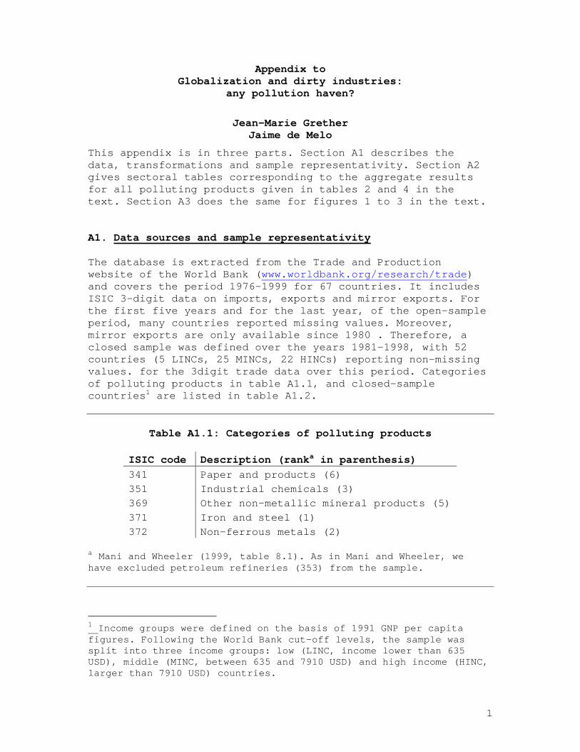
A1. Data sources and sample representativity
The database is extracted from the Trade and Productionwebsite of the World Bank (www.worldbank.org/research/trade)and covers the period 1976-1999 for 67 countries. It includesISIC 3-digit data on imports, exports and mirror exports. Forthe first five years and for the last year, of the open-sampleperiod, many countries reported missing values. Moreover,mirror exports are only available since 1980 . Therefore, aclosed sample was defined over the years 1981-1998, with 52countries (5 LINCs, 25 MINCs, 22 HINCs) reporting non-missingvalues. for the 3digit trade data over this period. Categoriesof polluting products in table A1.1, and closed-samplecountries1 are listed in table A1.2.
Table A1.1: Categories of polluting products
ISIC code Description (ranka in parenthesis)
341 Paper and products (6)
351 Industrial chemicals (3)
369 Other non-metallic mineral products (5)
371 Iron and steel (1)
372 Non-ferrous metals (2)
a Mani and Wheeler (1999, table 8.1). As in Mani and Wheeler, wehave excluded petroleum refineries (353) from the sample.
1 Income groups were defined on the basis of 1991 GNP per capitafigures. Following the World Bank cut-off levels, the sample wassplit into three income groups: low (LINC, income lower than 635USD), middle (MINC, between 635 and 7910 USD) and high income (HINC,larger than 7910 USD) countries.
2
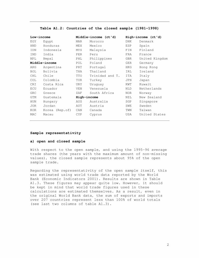
Table A1.2: Countries of the closed sample (1981-1998)
Low-income Middle-income (ct'd) High-income (ct'd)EGY Egypt MAR Morocco DNK DenmarkHND Honduras MEX Mexico ESP SpainIDN Indonesia MYS Malaysia FIN FinlandIND India PER Peru FRA FranceNPL Nepal PHL Philippines GBR United KingdomMiddle-income POL Poland GER GermanyARG Argentina PRT Portugal HKG Hong KongBOL Bolivia THA Thailand IRL IrelandCHL Chile TTO Trinidad and T. ITA ItalyCOL Colombia TUR Turkey JPN JapanCRI Costa Rica URY Uruguay KWT KuwaitECU Ecuador VEN Venezuela NLD NetherlandsGRC Greece ZAF South Africa NOR NorwayGTM Guatemala High-income NZL New ZealandHUN Hungary AUS Australia SGP SingaporeJOR Jordan AUT Austria SWE SwedenKOR Korea (Rep.of) CAN Canada TWN TaiwanMAC Macau CYP Cyprus USA United States
Sample representativity
a) open and closed sample
With respect to the open sample, and using the 1995-96 averagetrade shares (the years with the maximum amount of non-missingvalues), the closed sample represents about 95% of the opensample trade.
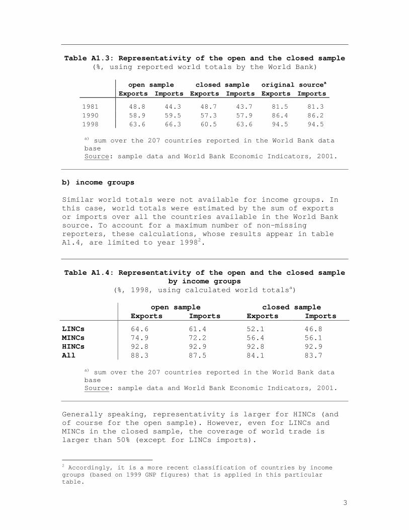
Regarding the representativity of the open sample itself, thiswas estimated using world trade data reported by the WorldBank (Economic Indicators 2001). Results are shown in TableA1.3. These figures may appear quite low. However, it shouldbe kept in mind that world trade figures used in thesecalculations are estimated themselves. As a result, even inthe original World Bank data, the sum of exports and importsover 207 countries represent less than 100% of world totals(see last two columns of table A1.3).
3
Table A1.3: Representativity of the open and the closed sample(%, using reported world totals by the World Bank)
open sample closed sample original sourcea
Exports Imports Exports Imports Exports Imports
1981 48.8 44.3 48.7 43.7 81.5 81.31990 58.9 59.5 57.3 57.9 86.4 86.21998 63.6 66.3 60.5 63.6 94.5 94.5
a) sum over the 207 countries reported in the World Bank databaseSource: sample data and World Bank Economic Indicators, 2001.
b) income groups
Similar world totals were not available for income groups. Inthis case, world totals were estimated by the sum of exportsor imports over all the countries available in the World Banksource. To account for a maximum number of non-missingreporters, these calculations, whose results appear in tableA1.4, are limited to year 19982.
Table A1.4: Representativity of the open and the closed sampleby income groups
(%, 1998, using calculated world totalsa)
open sample closed sampleExports Imports Exports Imports
LINCs 64.6 61.4 52.1 46.8MINCs 74.9 72.2 56.4 56.1HINCs 92.8 92.9 92.8 92.9All 88.3 87.5 84.1 83.7
a) sum over the 207 countries reported in the World Bank databaseSource: sample data and World Bank Economic Indicators, 2001.
Generally speaking, representativity is larger for HINCs (andof course for the open sample). However, even for LINCs andMINCs in the closed sample, the coverage of world trade islarger than 50% (except for LINCs imports).
2 Accordingly, it is a more recent classification of countries by incomegroups (based on 1999 GNP figures) that is applied in this particulartable.
4
c) polluting products
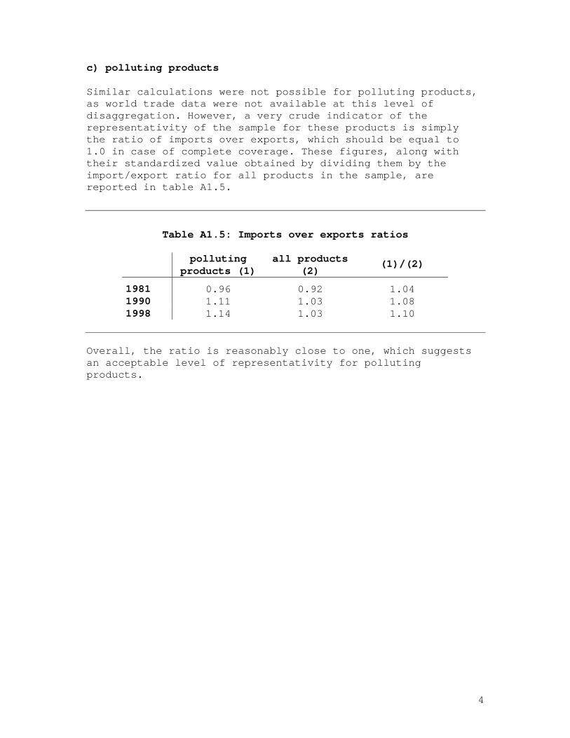
Similar calculations were not possible for polluting products,as world trade data were not available at this level ofdisaggregation. However, a very crude indicator of therepresentativity of the sample for these products is simplythe ratio of imports over exports, which should be equal to1.0 in case of complete coverage. These figures, along withtheir standardized value obtained by dividing them by theimport/export ratio for all products in the sample, arereported in table A1.5.
Table A1.5: Imports over exports ratios
pollutingproducts (1)
all products(2)
(1)/(2)
1981 0.96 0.92 1.041990 1.11 1.03 1.081998 1.14 1.03 1.10
Overall, the ratio is reasonably close to one, which suggestsan acceptable level of representativity for pollutingproducts.
5
A2. Sectoral results: tables
Table A2.1: Shares of developing countries in world trade
Paper and products (ISIC=341)
polluting products all products revealedcomparative
exports imports exports imports advantage disad-vantage
(1) (2) (3) (4) (1)/(3) (2)/(4)1981-83 3.70 12.70 9.40 15.73 0.39 0.811996-98 9.55 19.92 15.93 18.67 0.60 1.07rate of growth 6.53 3.05 3.58 1.15
Industrial chemicals (ISIC=351)
polluting products all products revealedcomparative
exports imports exports imports advantage disad-vantage
(1) (2) (3) (4) (1)/(3) (2)/(4)1981-83 5.11 21.55 9.40 15.73 0.54 1.371996-98 12.12 24.33 15.93 18.67 0.76 1.30rate of growth 5.92 0.82 3.58 1.15
Other non-metallic mineral products (ISIC=369)
polluting products all products revealedcomparative
exports imports exports imports advantage disad-vantage
(1) (2) (3) (4) (1)/(3) (2)/(4)1981-83 11.42 22.33 9.40 15.73 1.22 1.421996-98 16.28 19.16 15.93 18.67 1.02 1.03rate of growth 2.39 -1.02 3.58 1.15
Iron and steel (ISIC=371)
polluting products all products revealedcomparative
exports imports exports imports advantage disad-vantage
(1) (2) (3) (4) (1)/(3) (2)/(4)1981-83 9.09 23.63 9.40 15.73 0.97 1.501996-98 18.38 26.85 15.93 18.67 1.15 1.44rate of growth 4.81 0.86 3.58 1.15
Non-ferrous metals (ISIC=372)
polluting products all products revealedcomparative
exports imports exports imports advantage disad-vantage
(1) (2) (3) (4) (1)/(3) (2)/(4)1981-83 24.01 10.31 9.40 15.73 2.56 0.661996-98 22.91 17.88 15.93 18.67 1.44 0.96rate of growth -0.31 3.73 3.58 1.15
6
Table A2.2: Decomposition of aggregate change in RCA for LDCs
ISICCategory
total changein RCA
compositioneffect
structuraleffect
341 0.206 -0.060 0.266351 0.216 -0.087 0.303369 -0.193 -0.301 0.108371 0.186 -0.260 0.446372 -1.118 -0.529 -0.589
Table A2.3 : Gravity equation: Hausman-Taylor estimatesDependent variable: Mijt (imports of i from j in period t)
MijtIndependent POL2-HT 341b 351c 369 371 372ln (Yit) 1.50** 1.26** 1.27** 1.69** 1.82** 1.91**
(19.4) (12.6) (16.39) (15.4) (16.5) (17.8)ln (Yjt) 0.92** 0.58 1.86** -0.58** -0.32* -0.16
(10.9) (5.0) (21.8) (5.0) (2.5) (1.3)ln[(Yit/Nit) - 0.007 0.08* 0.03 0.12** 0.11** -0.04
(Yjt/Njt)] (0.3) (2.0) (1.1) (3.5) (2.7) (1.1)Ln DISTij -1.12** -1.40** -1.23** -1.21** -1.12** -0.95**
(17.7) (14.4) (19.1) (12.9) (7.9) (6.8)BORij 1.30** 1.68** 1.15** 1.70** 0.96** 0.87
(5.5) (4.01) (4.6) (4.2) (2.8) (1.6)LLi 0.49 0.52 -0.28 1.76** 2.79** 2.26**
(1.66) (1.0) (0.9) (3.4) (4.23) (3.3)LLj -0.42** -2.48** -1.99** -4.39** -3.79** -2.48**
(1.22) (3.8) (5.4) (6.9) (4.25) (3.3)Ln INFit 0.46** 0.48** 0.43** 0.98** 0.51** 0.55**
(6.43) (5.1) (6.1) (9.3) (4.4) (4.9)Ln INFjt 0.64** 1.19** 0.26** 2.22** 1.43** 0.15
(7.7) (9.9) (3.0) (18.6) (9.9) (1.2)Ln RERijt -0.40* -0.57** -0.35** -0.66** -0.71** -0.19**
(14.3) (14.3) (12.6) (16.3) (16.6) (5.1)Number of obs (NT) 30345 21831 28087 20907 21122 21591
Number of bilateral (N) 2300 2017 2240 1970 1938 1956
R² 0.52 0.51 0.52 0.44 0.51 0.35
Hausman test HT vs. GLS 614.7** 413.1** 589.6** 13.7** 97.9** 182.5**
chi-2(K) Chi-2(25) Chi-2(25) Chi-2(25) Chi-2(25) Chi-2(25) Chi-2(25)
** and *: significant at 99% and 95% respectively (t-student underthe correspondent coefficient)Time dummy variables and constant term not reported .Random effect estimates (endogenous variables : Yi and Yj and (Yi/Ni -Yj/Nj))
7
A3.
Sectoral
results:
figures
A3.1:Histograms
for
Output
(shout)Consumption
(shcon)Exports
(shmex)
andImports
(shimp)
(1:
beginning,
2:
end
of
period)
isic
=341
0255075 s
him
p1 s
him
p2
12
34
5is
ic=3
410255075
shm
ex1
shm
ex2
12
34
5
isic
=341
0255075
sho
ut1
sho
ut2
12
34
5is
ic=3
410255075
shc
on1
shc
on2
12
34
5
8
A3.1:Histograms
for
Output
(shout)Consumption
(shcon)Exports
(shmex)
andImports
(shimp)
(1:
beginning,
2:
end
of
period)
(cont'd)
isic
=351
0255075 s
him
p1 s
him
p2
12
34
5is
ic=
351
0255075 s
hmex
1 s
hmex
2
12
34
5
isic
=351
0255075 s
hout
1 s
hout
2
12
34
5is
ic=
351
0255075 s
hcon
1 s
hcon
2
12
34
5
9
A3.1:Histograms
for
Output
(shout)Consumption
(shcon)Exports
(shmex)
andImports
(shimp)
(1:
beginning,
2:
end
of
period)
(cont'd)
isic
=36
90255075
shi
mp1
shi
mp2
12
34
5is
ic=
369
0255075 s
hmex
1 s
hmex
2
12
34
5
isic
=369
0255075 s
hout
1 s
hout
2
12
34
5is
ic=
369
0255075 s
hcon
1 s
hcon
2
12
34
5

10
A3.1:Histograms
for
Output
(shout)Consumption
(shcon)Exports
(shmex)
andImports
(shimp)
(1:
beginning,
2:
end
of
period)
(cont'd)
isic
=371
0255075 s
him
p1 s
him
p2
12
34
5is
ic=3
710255075
shm
ex1
shm
ex2
12
34
5
isic
=371
0255075 s
hout
1 s
hout
2
12
34
5is
ic=3
710255075
shc
on1
shc
on2
12
34
5
11
A3.1:Histograms
for
Output
(shout)Consumption
(shcon)Exports
(shmex)
andImports
(shimp)
(1:beginning,
2:
end
of
period)(end)
isic
=372
0255075 s
him
p1 s
him
p2
12
34
5is
ic=3
720255075
shm
ex1
shm
ex2
12
34
5
isic
=372
0255075 s
hout
1 s
hout
2
12
34
5is
ic=3
720255075
shc
on1
shc
on2
12
34
5
12
A3.2: Beginning(1) and End(2) of period RCAs, by country group
ISIC = 341
RCAs based on MEXP - LINC + MINCrank
rca1 rca2
0 10 20 30
0.00
1.00
2.00
3.00
4.00
CHL
PRT
ZAF
MAR
MEXURY POL
GRC COL NPL KOR CRI ARG JOR PHL THA ECU HUN TTO VEN MYS HND IDN BOL IND MACTUR PER EGY GTM
CHL
PRT
IDN
ZAF
POLCOL
URYJOR
ARG CRI KOR HUN TTO VEN GTMGRCECU
THA BOL MARHND EGY NPL TUR MYSMEX PHLIND MACPER
RCAs based on MEXP - HINCrank
rca1 rca2
0 10 20
0.00
5.00
10.00
15.00
FIN
SWECAN
NOR
AUT NZL
CYP USA ESP NLD GER FRA DNK GBR ITA IRL TWN JPN AUS HKG SGP KWT
FIN
SWE
CAN NOR
AUT NZL
USA NLD GER ESP FRA ITA GBR DNK CYP AUS HKG TWN JPN IRL SGP KWT
13
A3.2: Beginning(1) and End(2) of period RCAs, by country group(cont'd)
ISIC = 351
RCAs based on MEXP - LINC + MINCrank
rca1 rca2
0 10 20 30
0.00
10.00
20.00
30.00
MAR
ZAFJOR TTO MEX HUNGTMPOL PRT NPL COL ARG CHL URY KOR TUR HND VEN PERGRC BOL CRI IND PHL THA MYS IDN EGY ECU MAC
JOR
TTO
MARCOL
KOR VEN ZAFIND
POL IDN HUN CHL GRCURY ARGGTMTUR PRT MEX THA EGY PER CRI MYS BOL ECU NPL PHL HNDMAC
RCAs based on MEXP - HINCrank
rca1 rca2
0 10 20
0.00
5.00
10.00
NLD
GER NOR IRL GBRUSA FRA
AUT CAN
ITA ESP
FIN AUS SWE JPN DNK TWN
NZL SGP CYP KWT HKG
IRL
NLD
NOR
GER GBR FRAUSA
TWNESP
AUT JPN CAN ITAFIN SGP KWT NZL DNK
CYP SWEAUS
HKG

14
A3.2: Beginning(1) and End(2) of period RCAs, by country group(cont'd)
ISIC = 369
RCAs based on MEXP - LINC + MINCrank
rca1 rca2
0 10 20 30
0.00
1.00
2.00
3.00 GRC
JOR
COL
TUR
KOR PRTCRI
THA MEXMAR PHL POL PER URY ZAF IND HUNGTM IDN MYSHND ARG CHL ECU VEN NPL MAC BOL TTO EGY
JOR
GRC
TUR COL
VEN
POL PRT INDURY EGY MEX CHL HUN TTO THA ECUMAC ZAF GTMPER MAR IDN CRI KOR MYS HND PHL ARG BOL NPL
RCAs based on MEXP - HINCrank
rca1 rca2
0 10 20
0.00
0.50
1.00
1.50 ESPCYP
ITA
AUT
DNK
GER FRATWN JPN IRL KWT GBR NLD
CAN NOR SWE USA SGP AUS NZL FINHKG
ESP
ITA
CYP
AUT
DNK
FRA GER NOR CAN GBR NLD AUSFIN JPN SWE
TWN USAIRL
HKG NZL SGP KWT

15
A3.2: Beginning(1) and End(2) of period RCAs, by country group(cont'd)
ISIC = 371
RCAs based on MEXP - LINC + MINCrank
rca1 rca2
0 10 20 30
0.00
2.00
4.00
6.00
8.00
ZAF
KOR
POLTUR
GRCHUN
VENGTMARGMEX TTO JOR IND PRT
IDN EGY COL CHL PHL THA PER URY MYS CRI HND BOL MARMACECU NPL
ZAF
ARG
TTO
TUR
VEN
POL
KORGRC COL EGY
IND
GTMMEXHUN
PRT IDN THA CRI CHL URY MYS PER JOR ECU NPL PHL MAR HNDMACBOL
RCAs based on MEXP - HINCrank
rca1 rca2
0 10 20
0.00
1.00
2.00
3.00
4.00
ESP
JPN
AUT
NOR
SWEFRA
GERFIN ITA
AUS
GBR NLDKWT CAN
TWN
DNK USA
SGP NZLIRL CYP HKG
NOR
AUTFIN SWE
AUS
ESPJPN FRA
GERITA
GBRNLD CYP TWN
CAN DNKNZL
USA
SGP IRL HKGKWT

16
A3.2: Beginning(1) and End(2) of period RCAs, by country group(end)
ISIC = 372
RCAs based on MEXP - LINC + MINCrank
rca1 rca2
0 10 20 30
0.00
10.00
20.00
BOLCHL
PER
ZAF
IDN
EGY ARG THAPOL MYSMEX VEN
GRCMARPHL HUNTUR URY CRI KORGTM TTO COL PRT ECU NPL IND JOR HNDMAC
CHL
PER
ZAF
BOL
VEN
GRC
POL EGY
IDN HUNMEX PHL TUR JOR MAR TTO IND KOR ARG CRI MYS COL URY THA ECU PRT NPL GTMMACHND
RCAs based on MEXP - HINCrank
rca1 rca2
0 10 20
0.00
5.00
10.00
15.00
AUS
NOR
CAN
NZLFIN ESP GBR NLD AUT SWE GER FRA USA
ITA JPN DNK HKG SGP TWN IRL CYP KWT
FIN
SWE
CAN NOR
AUT NZL
USA NLD GER ESP FRA ITA GBR DNK CYP AUS HKG TWN JPN IRL SGP KWT


