
N94- 35867
MANEUVERING AND CONTROL OF FLEXIBLE SPACE ROBOTSf
Leonard Meirovitch _' and Seungchul Lim**
Department of Engineering Science and Mechanics
Virginia Polytechnic Institute and State University
Blacksburg, VA 24061
) - __. //
g.o. 18"
SUMMARY
This paper is concerned with a flexible space robot capable of maneuvering payloads. The
robot is assumed to consist of two hinge-connected flexible arms and a rigid end-effector holding
a payload; the robot is mounted on a rigid platform floating in space. The equations of motion are
nonlinear and of high order. Based on the assumption that the maneuvering motions are one order
of magnitude larger than the elastic vibrations, a perturbation approach permits design of controls
for the two types of motion separately. The rigid-body maneuvering is carried out open loop, but
the elastic motions are controlled closed loop, by means of discrete-time linear quadratic regulator
theory with prescribed degree of stability. A numerical example demonstrates the approach. In the
example, the controls derived by the perturbation approach are applied to the original nonlinearsystem and errors are found to be relatively small.
1. INTRODUCTION
A variety of space missions can be carried out effectively by space robots. These missions
include the collection of space debris, recovery of spacecraft stranded in a useless orbit, repair of
malfunctioning spacecraft, construction of a space station in orbit and servicing the space station
while in operation. To maximize the usefulness of the space robot, the manipulator arms should be
reasonably long. On the other hand, because of weight limitations, they must be relatively light.
To satisfy both requirements, the manipulator arms must be highly flexible. Hence, space robots
share some of the dynamics and control technology with articulated space structures.
Robotics has been an active research area for the past few clecades, but applications have been
concerned primarily with industrial robots, which are ground based and tend to be very stiff and
bulky. In contrast, space robots are based on a floating platform and tend to be highly flexible.
Hence, whereas industrial and space robots have a number of things in common, the differences are
significant. More recent investigations have been concerned with flexible industrial robots (Refs.
1-4). On the other hand, some investigations are concerned with space robots consisting of rigid
links (Refs. 5-7). Research on flexible space robots has come to light only recently (Refs. 8,9).
l Research supported by the NASA Research Grant NAG-I-225 monitored
Montgomery. The support is greatly appreciated.* University Distinguished Professor
** Graduate Research Assistant
by Dr. R.C.
23
https://ntrs.nasa.gov/search.jsp?R=19940031360 2020-05-15T18:15:26+00:00Z

'['his paper is concerned with a flexible space robot capable of maneuvering payloads. The
robot is assumed to consist of two hinge-connected flexible arms and a rigid end-effector holding
a payload; the robot is mounted on a rigid platform floating in space (Fig. 1). Tile platform
is capable of translations and rotations, tile flexible arms are capable of rotations and elasticdeformations and the end-effector/payload can undergo rotations relative to the connecting flexible
arm. Based on a consistent kinematical synthesis, the motions of one body in the chain take into
consideration the motions of the preceding body in the chain. This permits the derivation of the
equations of motion without the imposition of constraints. The equations of motion are derived by
the Lagrangian approach. The equations are nonlinear and of relatively high order.
Ideally, the maneuvering of payloads should be carried without exciting elastic vibration,
which is not possible in general. However, the elastic motions tend to be small compared to the
rigid-bodv maneuvering motions. Under such circumstances, a perturbation approach permits
separation of the problem into a zero-order problem (in a perturbation theory sense) for the
rigid-body maneuvering of the space robot and a first-order problem for the control of the elasticmotions and the perturbations from the rigid-body motions. The maneuvering can be carried out
open loop, but the elastic and rigid-body pert,rbations are controlled closed loop.
The robot mission consists of carrying a payload over a prescribed trajectory and placing it
in a certain orientation relative to the inertial space. For planar motion, the end-effector/payload
configuration is defined by three variables, two translations and one rotation. At the end of the
mission, the vibration should be damped out, so that the robot can be regarded as rigid at that
time. Still, the rigid robot possesses six degrees of freedom, two translations of the platform and
one rotation of each of the four bodies, including the platform. This implies that a kinematic
redundancy exists. This redundancy is removed in the trajectory planning so as to conserve fuel.
For a given end-effector/payload trajectory, the rigid-body maneuvering configuration of the
robot can be obtained by means of inverse kinematics. Then, the forces and torques required for
the robot trajectory realization are obtained from the zero-order equations by means of inverse
dynamics.
The first-order equations for the elastic motions and the perturbations in the rigid-body
maneuvering motions are linear, but of high order, time-varying and they are subjected to
persistent disturbances. The persistent disturbances are treated by means of feedforward control.
All other disturbances are controlled closed loop, with the feedback controls being designed by
means of discrete-time linear quadratic regulator (LQR) theory with prescribed degree of stability.
A numerical example demonstrates the approach. In the example, the controls derived by the
perturbation approach are applied to the original nonlinear system and the errors in the end-
effector/payload configuration were found to be relatively small during the maneuver and to vanish
soon after the termination of the maneuver.
2. A CONSISTENT KINEMATICAL SYNTHESIS
To describe the motion of the space robot, it is convenient to adopt a consistent kinematical
synthesis whereby the system is regarded as a chain of bodies and the motion of one body is
24

definedwith dueconsiderationto the motionof the preceedingbody in the chain.Figure 1 showsthe mathematicalmodelof thespacerobot, consistingof a rigid platform (Body 1), two hinge-connectedflexiblearms(Bodies2 and 3) and a rigid end-effectorholdingthe payload(Body4).The variousmotionsare referredto a setof inertial axesand setsof body axesto bedefinedshortly.
The object is to derivethe systemequationsof motion,whichcanbedoneby meansofLagrange'sequationsin termsof quasi-coordinates(Ref. 10). Becausein the caseat hand themotion is planar, it is moreexpedientto usethestandardLagrange'sequations.This requiresthekinetic energy,potential energyand virtual work. The kinetic energy,in turn, requiresthe velocityof a typical point in eachof the bodies.
The positionof a nominalpoint on the platformis givenby
RI = R0+ rl (1)
whereR0 = [X y]T is the position vector of the origin Ox of the body axes xl,yz (Fig. I) relative
to the inertial axes X, Y and in terms of X, Y components and rl = [xl yl] T is the position
vector of the nominal point on the platform relative to the body axes xl,yl and in terms of zl,yl
components. The velocity vector of a point on the platform can be expressed in terms of xl,ylcomponents as follows:
Vl = Clfto + &lrl (2)
where
C1 = [ cO1 sol]
__sO 1 CO 1 j (3)
is a matrix of direction cosines between axes Zl,yl, and X, Y, in which sO1 = sinOl, c01 = cos 01,
R0=[x ?it (4)
is the velocity vector of Ol in terms of X, Y components and
0 -b,]{'7)1= 01 0 (5)
The second body is flexible, so that we must resolve the question of body axes. We define the
body axes z2, Y2 as a set of axes with the origin at the hinge 02 and embedded in the undeformed
body such that x2 is tangent to the body at 02 (Fig. 2). Then, we define the motion of axes z2, Y2
as rigid-body motion and measure the elastic motion relative to x2, Y2- Hence, the velocity of a
point in the second body (first flexible arm) in terms of z2, y-q components is
V 2 _.-_C2_IV1 (02) Ar t_-q(g2 q- u-q) -_-1_12rel
=C21_0 + C2_lCblrl (02) + ¢b-q(t"2 + u q) + fl2rel (6)
where C2-1 and C2 are matrices similar to CI, Eq. (3), except that 01 is replaced by 02 -- 01 and
02, respectively, _2 has the same structure as &l but with 02 replacing 01, rl(O-q) = [dl hl] T, r2 =
25

[.r2 0] T, u2 = [0 U2]T and fl2,el = [0 h2], in which u2 = u2(x2, t) and/t2 = it2(x2, t) are the elastic
displacement and velocity, respectively.
Using the analogy with the second body, the velocity of a point in the third body (second
flexible arm) in terms of z3, y3 components can be shown to be
V3 =C3-2V2(L_.) + w3(r3 + u3) + U3rel
=C3 + cs_iCOlr (o..)+ cs-2 {co2[r2(L2)+ u2(L2,t)l+ 62re|(L2,t)}
+ w3(r3 + u3) + fl3ret(7)
The fourth body consists of the end-effector and payload combined, and is treated as rigid.
Following the established pattern, the velocity of a point in the fourth body in terms of z4, y4
components is
V 4 =CI_3V3(L3) + _4r4
=C41_0 + C4-1wlrl(O_.) + C4-2 {w2 [r2(L2) + u_.(L2, t)] + fl2r¢l(L2,t)}
"4- C4-3 {_z [r3(L3) + u3(L3, t)] + l_13rel(L3,/:)} 4- &4r4(8)
The consistent kinematical synthesis just described permits the formulation of the equations
of motion for the whole system without invoking constraint equations. Such constraint equations
must be used to eliminate redundant coordinates in a formulation in which equations of motion are
derived separately for each body.
3. SPATIAL DISCRETIZATION OF THE FLEXIBLE ARMS
The velocity expressions derived in Sec. 2 involve rigid-body motions depending on time
alone and elastic motions depending on the spatial position and time. Equations of motion
based on such formulations are hybrid, in the sense that the equations for the rigid-body motions
are ordinary differential equations and the ones for the elastic motions are partial differential
equations. Designing maneuvers and controls on the basis of hybrid differential equations is likely
to cause serious difficulties, so that the only viable alternative is to transform the hybrid system
into one consisting of ordinary differential equations alone. This amounts to discretization in space
of the elastic displacements, which can be done by means of series expansions. Assuming that the
flexible arms act as beams in bending, the elastic displacements can be expanded in the series
rti
= i= 2,3 (9)j=l
where ckij(xi) are admissible functions, often referred to as shape functions, and r/ij(t) are
generalized coordinates; 4'j and r/i are corresponding ni-dimensional vectors (i = 2,3; j =
1,2,...,ni)
The question arises as to the nature of the admissible functions. Clearly, the object is to
approximate the displacements with as few terms in the series as possible. This is not a new
26

problemin structural dynamics, and tile very same subject has been investigated recently in
Ref. 11, in which a new class of functions, referred to as quasi-comparison functions, has been
introduced. Quasi-comparison functions are defined as linear combinations of admissible functions
capable of satisfying the boundary conditions of the elastic member. As shown in Fig. 2, the beam
is tangent to axis zi at Oi(i = 2, 3). Hence, the admissible functions must be zero and their slope
must be zero at zi = 0. At zi = Li, the displacement, slope, bending moment and shearing force
are generally nonzero. Quasi-comparison functions are linear combinations of functions possessing
these characteristics. Admissible functions from a single family of functions do not possess the
characteristics, but admissible functions from several suitable families can be combined to obtain
them. In the case at hand, quasi-comparison functions can be obtained in the form of suitable
linear combinations of clamped-free and clamped-clamped shape functions.
4. LAGRANGE'S EQUATIONS
Before we can derive Lagrange's equations, we must produce expressions for the kinetic energy,potential energy and virtual work. To this end, and following the spatial discretization indicated
by Eqs. (9), we introduce the configuration vector
q(t) = Ix(t) K(t) O,(t)O2(t)03(t) 04(t),T(t) r/T(t)] T
so that the velocity vectors, Eqs. (2), (6)-(8), can be written in the compact form
(10)
Vi = Dig:l, i = 1,2,3,4 (11)
where
cO1 s01 --1Jl 0 ... 0 T]D1 = _s01 cO 1 Zl 0 ... 0 T
s02 d18(02 - 01) - hlC(02 - 01)D2= cO2d,c(o -oi)+hl (o -o1)-¢r,h o o or oT]
z2 0 0 q_T 0TJ (12)
Then, the kinetic energy is simply
where
vTv,..,-le,..4
is the mass matrix. Typical entries in tile mass matrix are
(13)
(14)
roll ----rrt, rnl2 ---- 0, m13 ----- --(m 2 + m 3 + m4)(hlc01 + dis01)
................................. , ............
27

m22 =re, m23 = --(m2 + rn3 + m4)(hlSOl - dlcO1)
ms8 =/Body 3 ¢3¢rdm3 + m463(L3)¢T(L3)
(15)
in which
' Lm = _ mi, _i = /m dPidmi' i = 2, 3, Si = xidmi, i = 1,2,3,4 (16)i i
i=1
The potential energy, assumed to be entirely due to bending, has the form
1 L2 _. lf0ts
in which Eli(i = 2, 3) are bending stiffnesses and primes denote spatial derivatives, lVloreover,
K = block - diag[0 K2 Ks] (18)
is the stiffness matrix, where
fO Li tt . TIQ = Elid_i (c_i) dzi, i=2,3 (19)
are stiffness matrices for the flexible arms.
Next, we propose to derive the virtual work expression. To this end, we must specify first the
actuators to be used. There are three actuators acting on the platform, two thrusters Fzl and
Fyl acting in directions aligned with tile body axes and a torquer M1 acting at O1. Three other
torquers M2, Ms and 344 are located at the hinges 02, Oa and 04, respectively, the first acting on
the platform and first arm, the second acting on the first and second arm and the third acting on
the second arm and end-effector. In view of this, the virtual work can be written as follows:
6W =F=I (cosOl6X + sin 016Y') + F_,I (-sinO16X + cosOl6Y) + M1601
+ M26(02 - 0,) + M36,1's + M46¢4 + Ms6 [02 + _b_T (L_/3) rt2]
where 6X, 6Y,... are virtual displacements. Moreover, denoting the angles between the two arms
and between the second arm and the end-effector by
I =0s__bs =03 - 02 - Oz21,2=L_ (21)
I = 0,__b4 =04 - 03 - Ozs I_.s=L3
28

wecanwrite6_3 -----603 --_02 --_b"T(L2)6.2 , _b 4 ---604 - 603 - _b3r/"(L3)6,h (22)
Inserting Eqs. (22) into Eq. (20), we can express the virtual work in terms of generalized forces
and generalized virtual displacements in the form
6|V = QT6q (23)
where Q = [Fx Fy (91 O2 03 @4 N T NT] T is the generalized force vector, in which
FX =Fxl cos01 - Fvl sin 01, Fy = F_I sin01 + Fyl cos01
6)a =11¢1 - M2, 6)2 = M2 - M3 + 1115+ M6
O3 =M3 - M4 + 1117+ Ms, O4 = M4 (24)
N2 =Mhdp'2( L2/3 ) + M6¢'2(2L2/3) - M3(;b_(L2)
r% =MT¢ (L3/3) + Ms¢, (2L3/3)- M4¢ (L3)
and 6q = [6X 6Y 60_ 602 603 604 6rl T 6rIT] T is the generalized virtual displacement vector.
Equations (24) express the generalized forces and torques in terms of the actual actuator forces
and torques and can be expressed in the compact form
Q = EF
where F = [Fzl Fvl 1141 1112 ... Ms] T is the actual control vector and
E = E(O,)=cos01 -sin01
sin01 cos01
0 0
0 0
0 0
0 0
0 0
0 0
0 0 0 0 0 0 0
0 0 0 0 0 0 0
1 -1 0 0 0 0 0
0 1 -I 0 1 1 0
0 0 1 -1 0 0 1
0 0 0 1 0 0 0
o o -¢2(-) o o_%t-U)
0 0 0 -¢3(L3) 0 0 ¢
is a time-varying coefficient matrix, because 01 varies with time.
Lagrange's equation can be expressed in the general symbolic vector form
d(OT) OT OVd-t 0-_-_qq+-_q =Q
(25)
0
0
0
0
1
0
0
26)
(27)
29

Observingthat M = M(q), we can write
-gi o;a]07" 1.TOM. OV _ Kq
o--4q' 0q
Inserting Eqs. (28) into Eq. (27), we obtain Lagrange's equations in the more explicit form
1 _tTOM_/lift+ M-_ --ffq-q]Ct+Kq=Q
in which
6+2n OM. (:tTOM?S =--q,, -Nq=j=l i')qj
_tT OM / Oql
(:ITOM / Oq2
;:tr oqlli/ Oq6+ 2n
(28)
(29)
(30)
5. A PERTURBATION APPROACtI TO THE CONTROL DESIGN
Equation (29) represents a high-order system of nonlinear differential equations, and is not
very suitable for control design. Hence, an approach capable of coping with the problems of high-
dimensionality and nonlinearity is highly desirable. Such an approach must be based on the
physics of the problem. Tile ideal maneuver is that in which the robot acts as if its arms were
rigid. In reality, the arms are flexible, so that some elastic vibrations are likely to take place. It
is reasonable to assume, however, that the elastic motions are one order of magnitude smaller
than the maneuvering motions. This permits treatment of the elastic motions as perturbations
on the maneuvering motions. In turn, the elastic perturbations give rise to perturbations in the
"rigid-body" maneuvering motions. This suggests a perturbation approach, whereby the problem
is separated into a zero-order problem for the "rigid-body" maneuvering of the payload and a
first-order problem for the control of the elastic motions and the perturbations in the rigid-body
maneuvering motions. The zero-order problem is nonlinear, albeit of relatively low dimension. It
can be solved independently and the control can be open loop. On the other hand, the first-order
problem is linear, but of relatively high dimension. It is affected by the solution to the zero-order
problem, where the effect is in the form of time-varying coefficients and persistent disturbances.
The control for the first-order problem is to be closed loop.
We consider a first-order perturbation solution characterized by
q=q0+ql, Q=Q0+Q1 (31)
where the subscripts 0 and 1 denote zero-order and first-order quantities, with the zero-order
quantities being one order of magnitude larger than the first-order ones. Inserting Eqs. (31) into
Eq. (29) and separating quantities of different orders of magnitude, we obtain the equation for the
zero-order problem
- _M_ ) el0 = Q0 = EoF0Moqo + (My 1 T (32)
3O
whereqo = [Xo Yo 01o 0_o03o 04o 0 TOT] T, Qo = [Fxo Fxo Olo 020 O3o O4o0 TOT] Tare
zero-order displacement and generalized control vectors, Eo = E(01o) is the matrix E, Eq. (26),
evaluated at 01 = 01o, Fo = [F_o Fyo Mlo M2o ... Mso] T and
[OM. OM OM ]1M0=M(q0), M,= -_-qlq0 _q2dl0 ... 0q6+2,zdt0 q=q0
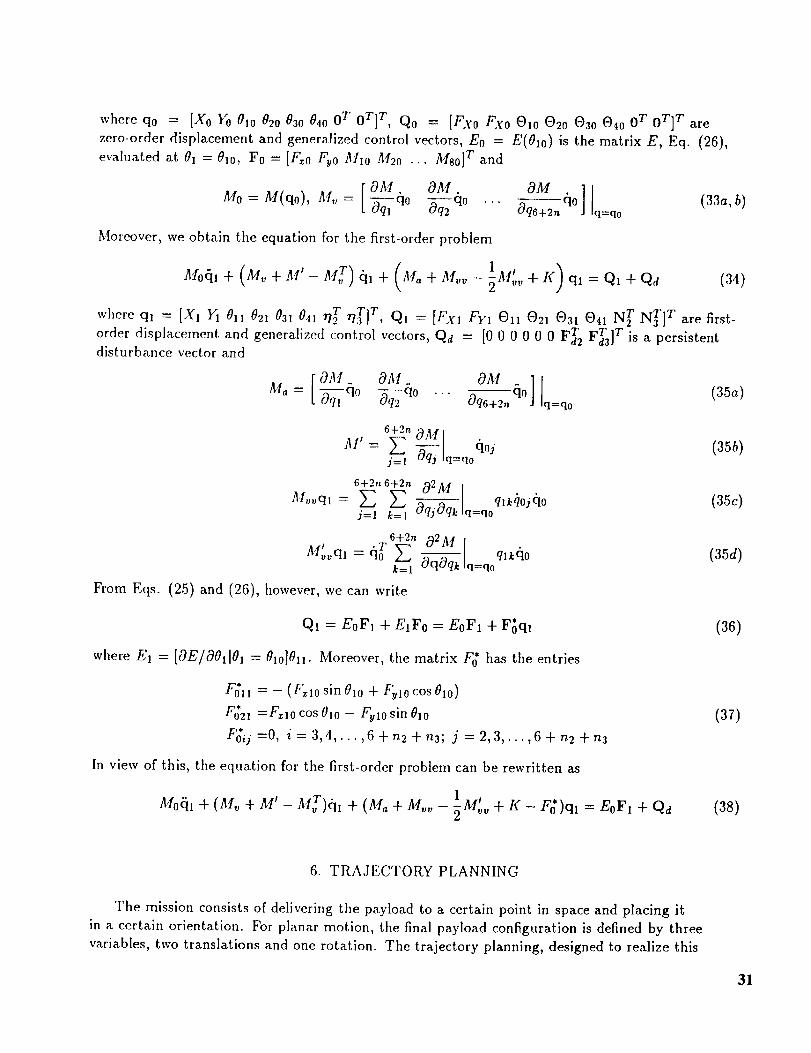
Moreover, we obtain the equation for the first-order problem
M0_ll + + M I _ M f ) fil
TTwhere q] = IX, Y1 011 021 03, 041 r/T r/3 ] , Q] = [Fx] Fy1 011 G21 031 041 N T NT] T are first-
order displacement and generalized control vectors, Qa = [0 0 0 0 0 0 F_r_FaT]r is a persistentdisturbance vector and
[ OM .. 03t .. 031]1M,
6+.o. OM
M'= _ -_qj iq=qoqOi (35b)j=l
6+2n 6+2n 02M
Iq qoqlkOOjfiO (35e)/_/ovql = E Z OqjOqk =j=l k=l
6+2n
02M I q]kdto (35d)M'_,ql = dl0T _ OqOqk q=qok=l
From Eqs. (25) and (26), however, we can write
Q1 = EoF1 + EIFo = EoF1 + F_ql (36)
where E1 = [0E/001101 = 0to]011. Moreover, the matrix F_ has the entries
F_11 = - (F_10 sin 010 + Fy]0 cos 010)
F_21 =Fzl0 cos 01o - FuI0 sin 010 (37)
F_i j =0, i=3,4,...,6+n2+n3; j=2,3,...,6+n2+n3
In view of this, the equation for the first-order problem can be rewritten as
1 iMo_tl + (M,, + M' - MT)(II + (M_, + M,,_, - -_M'_,v + I( - F_)qI = EoFI + Qd (38)
(33a, b)
6. TRAJECTORY PLANNING
The mission consists of delivering the payload to a certain point in space and placing it
in a certain orientation. For planar motion, the final payload configuration is defined by three
variables, two translations and one rotation. The trajectory planning, designed to realize this
31

final configuration, will be carried out as if the robot system were rigid, with the expectation thatall elastic motions and perturbations in the rigid-body maneuvering motions will be annihilated
by the end of the maneuver. The rigid-body motion of the robot is described by the zero-order
problem and it consists of six components, two translations of the platform and one rotationof each of the four bodies. This implies that a kinematical redundancy exists, as there is an
infinity of ways a six-dimensional configuration can generate a three-dimensional trajectory.
This redundancy can be removed by controlling three of the configuration variables, such as the
translations and rotation of the platform, so as to conserve fuel. Under these circumstances, the
rigid space robot can be treated as a nonredundant manipulator.
Next, we denote the end-effector configuration by XE, so that from kinematics we can write
XE = f(q0) (39)
where f is a three-dimensional vector function. From differential kinematics,
XE = J(q0)ct0
we have
(40)
whereJ(q0) = [Of/Oqo]
is the 3 x 6 Jacobian matrix. Introducing the notation
(41)
(42)
whereqs = IX0 ]do 010] T , qM = [020 030 040]T
are the controlled platform configuration vector and the open-loop controlled manipulator
configuration vector, and partitioning the Jacobian matrix accordingly, or
(43a, b)
J= [Js i JM] (44)
Eq. (40) can be rewritten asXE = Jsqs + JM¢tM (45)
Then, on the assumption that Cls is determined so as to minimize the fuel consumption, and for a
given end-effector trajectory XE, we can determine the manipulator velocity vector from
elm = JM 1 (XE- Jscts) (46)
The end-effector trajectory was taken in the form of a sinusoidal function so as to prevent excessive
vibration. Finally, with q0 given, we can obtain the required open-loop control F0 by inverse
dynamics, which amounts to using Eq. (32).
32

7. FEEDBACK CONTROL OF THE ELASTIC MOTIONS AND RIGID-BODY PERTURBATIONS
The elastic motions and the perturbations in the rigid-body maneuvering motions are governed
by the equation defining the first-order problem, Eq. (38). The persistent disturbances are
controlled open loop and all other disturbances are controlled closed loop. To this end, we expressthe control vector in the form
F1 = Flo +Flc (47)
where the subscripts o and c indicate open loop and closed loop, respectively. Recognizing that E0is a rectangular matrix, the open-loop control can be written as
in which
is the psuedo-inverse of Eo.
Flo = -EtoQd (48)
_-(E[Eo)-'Eo (49)
For tile closed-loop control, we consider a linear quadratic regulator (LQR), which requires
recasting the equations of motion in state form. Adjoining the identity ell = c11, the state
equations can be expressed as
_:(t) = A(t)x(t) + B(t)Eouc(t) + B(t)Dd(t) (50)
where x = [qT _tT]T is the state vector, u_ =FI¢ is the control vector, d = Qa is the disturbancevector and
[ 0 , ]_ 1 tA = _Mo_,(M_+ M_. _M_ + K- r_) -M_-_(M° + M'- Mr) (51_)
[ 0 1 ] D (I E0B= E_)
are coefficient matrices. It should be noted here that, if the matrix E0 is not square, the matrix
D is not zero, so that the open-loop control does not annihilate the persistent disturbances
completely. As the number of actuator approaches the number of degrees of freedom of the system,
the matrix E0 tends to become square. When the number of actuators coincides with the number
of degrees of freedom the matrix E0 is square, in which case the pseudo-inverse becomes an exactinverse and the matrix D reduces to zero.
The state equations, Eq. (50), possess time-varying coefficients and are subject to residual
persistent disturbances. Due to difficulties in treating such systems in continuous time, we propose
to discretize the state equations in time. Following the usual steps (Ref. 12), the state equations indiscrete time can be shown to be
where
xk+l = Ckxk + FkEot_Uck + FkDkdk, k = 0, I,...
xk =x(kT), u,k = u_(kT), dk = d(kT), k=0,1,...
¢k =exp AuT, Fk = (exp Aj, T- I)A-_IBk, k = O, I,...
Eok =Eo(kT), D_ = D(kT), k = 0,1,...
(52)
(53)
33

in which T is the sampling period. In view of the above discussion, we assume that the effect of
the persistent disturbances has been reduced drastically by the feedforward control, and design the
feedback control in its absence. This design is according to a discrete-time LQR with prescribed
degree of stability. To this end, we consider the performance measure
N-1TJ = xT,pN× + Z + (54)
k=0
where PN and Qk are symmetric positive semidefinite matrices, Rk is a symmetric positive definite
matrix, a is a nonnegative constant defining the degree of stability and NT is the final sampling
time.
The optimization process using the performance measure given by Eq. (54) can be reduced to
a standard discrete-time LQR form by means of the transformation
:xk = e_kxk, tick = e°&Uck, PN = e-_'aN pN (55a, b, e)
Multiplying Eqs. (52) through by eC'(k+l) using Eqs. (55a,b) and ignoring the small perturbing
term, we obtain the new state equations
z_k+t = e_' (_k_k + FkEokfiCk), k = 0,1,...,N - 1 (56)
Similarly, inserting Eqs. (55) into Eq. (54), we obtain the new performance measure
N-1^T Aj = + E + (57)
k=O
It can be shown (Ref. 12) that the optimal control law has the form
tick = Gk2k, k = 0, 1,...,N- 1 (58)
where Gk are gain matrices obtained from the discrete-time Riccati equations
2_ T T " E -1 2a T T= RN-i) e E 0 N_iFN_iPN+I-i_N-i,GN-i - (e E ON_iFN_iPN+I-iFN-i oN-i+
i = 1,2,... ,N;P = e-2aNpN (59a)
T . FIv_IEo,N-iGN-i),PN-i =e2a (_N-i + FN-iEo,N-iGN-i) PN+I-i (¢N-i +
+ GTIv_iRN_iGN-i + QN-i, i = 1,2,... ,N;Plv = e-2°_P_ (590
Equations (59a) and (59b) are evaluated alternately for GN-1, P1_-1, GN-2, Ply-2,..., Go, given
the final value of PN.
Inserting the control law, Eqs. (58), into Eqs. (56), we obtain the closed-loop transformed
state equations
_k+l = e'_ (_t, + FkE0kGk) z(k, k = 0,1,... (60)
34

Then,recallingEq. (55a) andrestoringthe persistentdisturbanceterm, the closed-loopstateequationsfor theoriginal systemcanbe written in the form
Xk+l = ('bk + FkE0kGk)xk+ FkDkdk, k = 0,1,... (61)
8. NUMERICAL EXAMPLE
The example involves tile flexible space robot shown in Fig. 1. Numerical values for the systemparameters are as follows:
L1 =1 m, dl = 0.5 m, L_ = L3 = 5m, L4 = 1.66m
ml =10 kg, m_ = m3 = lkg, m4 = 0.1 kg
J1 =20 kgm "_, J2 = 3 kgm 2, EI2 = EI3 = 122.28 Nm 2
The quasi-comparison functions for the flexible arm were chosen as a linear combination of
clamped-free and clamped-clamped shape functions. Both families of shape functions have tilefunctional form
1
¢i = _ [coshAiz/n - cos,\_xlt, - ai (sinh Jiz/Z - sinAix/Z)],i = 1,2,...,,_
The values of Ai and _ri are given in Table 1. They correspond to two clamped-free and three
clamped-clamped shape functions, for a total of n = 5 for each flexible arm.
The initial and final end-effector positions are defined by
Xi =9.757 m, I_ = 1.914 m, 04f = 0 rad
Xf =5.000 m, Y/= 1.914 m, 04I = 7r/2 rad
and we note that the path from the initial to the final position represents a straight-line
translation, while the orientation undergoes a 90 ° change. In terms of time, the translational and
rotational accelerations represent one-cycle sinusoidal curves.
The maneuver time is tf = 2.5 s. The zero-order actuator forces and torques to carry out the
maneuver are shown in Fig. 3.
The control of the elastic motions and the perturbations in the rigid-body motions was
extended to t = 4 s. Not that for 2.5 s < t < 4 s the system is time-invariant, during which time
the control gains can be regarded as constant. The weighting matrices in the performance measureare
Qt, = 10I, Rk = I, PN = 10I
The degree of stability constant is c_ = 0.1. Moreover, the samping period is T = 0.01 s and thenumber of time increments is N = 350.
Time-lapse plots of the uncontrolled and controlled robot configuration are shown in Figs. 4a
and 4b, respectively, at the instants 0, i, 1.5 and 2.5 s. Figures 5 and 6 show time histories of the
35

errorsin the end-effectorposition. The discrete-timeopen-loopandclosed-looppolesaregiveninTables2 and 3. For comparison,Fig. 7 showsthetime history of theerrorsandTable4 givestheclosed-looppolesfor a = 1.
It should be pointed out that tile actuator dynamics is also included in the formulation and the
numerical results, but the effect turned out to be small.
9. CONCLUSIONS
An orderly kinematic synthesis in conjunction with the Lagrangian approach permits the
derivation of the equations of motion for an articulated multibody system, such as those describing
the dynamical behavior of a flexible space robot, without the imposition of constraints. The
equations are nonlinear and of relatively high order. A perturbation approach permits the
separation of the problem into a zero-order problem (in a perturbation sense) for the rigid-body
maneuvering of the space robot and a first-order problem for the control of the elastic motions and
the perturbations from the rigid-body motions. The robot mission consists of carrying a payload
over a prescribed trajectory and placing it in a cerrtain orientation relative to the inertial space.
This represents the zero-order problem and the control can be carried out open loop. The first-
order equations defining tile first-order problem (in a perturbation sense) are linear, time-varying,
of high-order and subject to persistent disturbances. The persistent disturbances are treated by
means of feedforward control. All other disturbances are controlled closed loop, with the feedback
control being designed by means of discrete-time LQR theory with prescribed degree of stability.
In a numerical example, the controls derived by the perturbation approach are found to work
satisfactorily when applied to the original nonlinear system.
.
.
.
.
10. REFERENCES
Book, W.J., Maizza-Neto, A., and Whitney, D.E.: Feedback Control of Two Beam, Two Joint
Systems with Distributed Flexibility. ASME Journal of Dynamic Systems, Measurement, and
Control, vol. 97, Dec. 1975, pp.424-431.
Kozel, D. and Koivo, A.J.: A General Force/Torque Relationship and Kinematic
Representation for Flexible Link Manipulators. Journal of Robotic Systems, vol. 8, no. 4, 1991,
pp. 531-556.
Wang, D. and Vidyasagar, M.: Control of a Class of Manipulators with a Single FlexibleLink-Part 1: Feedback Linearization. ASME Journal of Dynamic Systems, Measurement, and
Control, vol. 113, Dec. 1991, pp. 655-661.
Nathan, P.J., and Singh, S.N.: Sliding Mode Control and Elastic Mode Stabilization of aRobotic Arm with Flexible Links. ASME Journal of Dynamic Systems, Measurement, and
Control, vol. 113, Dec. 1991.
36

5. Umetani,Y. and Yoshida,K.: ContinuousPathControl of SpaceManipulatorsMountedonOMV. Acta Astronautica, vol. 15, no. 12, 1987, pp. 981-986.
6. Nenchev, D., Umetani, Y., and Yoshida, K.: Analysis of a Redundant Free-Flying
Spacecraft/Manipulator System., IEEE Transactions on Robotics and Automation, vol. 8, no.1, 1992, pp. 1-6.
7. Nakamura, Y. and Mukherjee, R.: Nonholonomic Path Planning of Space Robots via a
Bidirectional Approach. IEEE Transactions on Robotics, and Automation, vol. 7, no. 4, 1991,pp. 500-514.
8. Usoro, P.B., Nadira, R., Mahil, S.S.: Control of Lightweight Flexible Manipulators: A
Feasibility Study. Proceedings of the American Control Conference, vol. 3, San Diego, CA,June 1984, pp. 1209-1216.
9. Meirovitch, L., Stemple, T., and I(wak, M.K.: Dynamics and Control of Flexible Space Robots.
Proceedings of the CSME Mechanical Engineering Forum, Toronto, Ontario, 1990.
10. Meirovitch, L.: Hybrid State Equations of Motion for Flexible Bodies in Terms of Quasi-
Coordinates. Journal of Guidance, Control, and Dynamics, vol. 14, no. 5, 1991, pp. 1008-1013.
11. Meirovitch, L. and Kwak, M.K.: Convergence of the Classical Rayleigh-Ritz Method and the
Finite Element Method. AIAA Journal, vol. 28, no. 8, 1990, pp. 1509-1516.
12. Kuo, B.C.: Digital Control Systems, SRL Publishing Co., Champaign, IL, 1977.
Table 1. Shape Function Coefficients
i
I
2
3
4
S
_-i al
1.87510407 0.734095514
4.69409113 1.018467319
7.85475744 0.999224497
10.99554073 1.000033553
14.13716839 0.999998550
Table 2. Discrete-Time Open-Loop Poles
NO.
1,2
3,4
5,6
7,8
9,10
11,12
13,14
lS,16 i
Pole Location Mag. No.
-0.840±0.5431 1.000 17,18
-0.778+0.6291 ! 1.000 19,20
-0.700_+0.714i 1.000 21,22
-0.690±0.724i 1.000 23,24
0.586±0.8101 1.000 25,26
0.629__0.7781 1.000 27,28
0.902__.0.431i .000 29,30
0.921+0.390i .000 31,32
Pole Location Mag.
0.991+0.135i 1.000
0.994_+0.107i 1.000
1.000 11.000
1.000 1.000
1.000 1.000
1.000 1.000
1.000 1.000
1.000 1.000
37
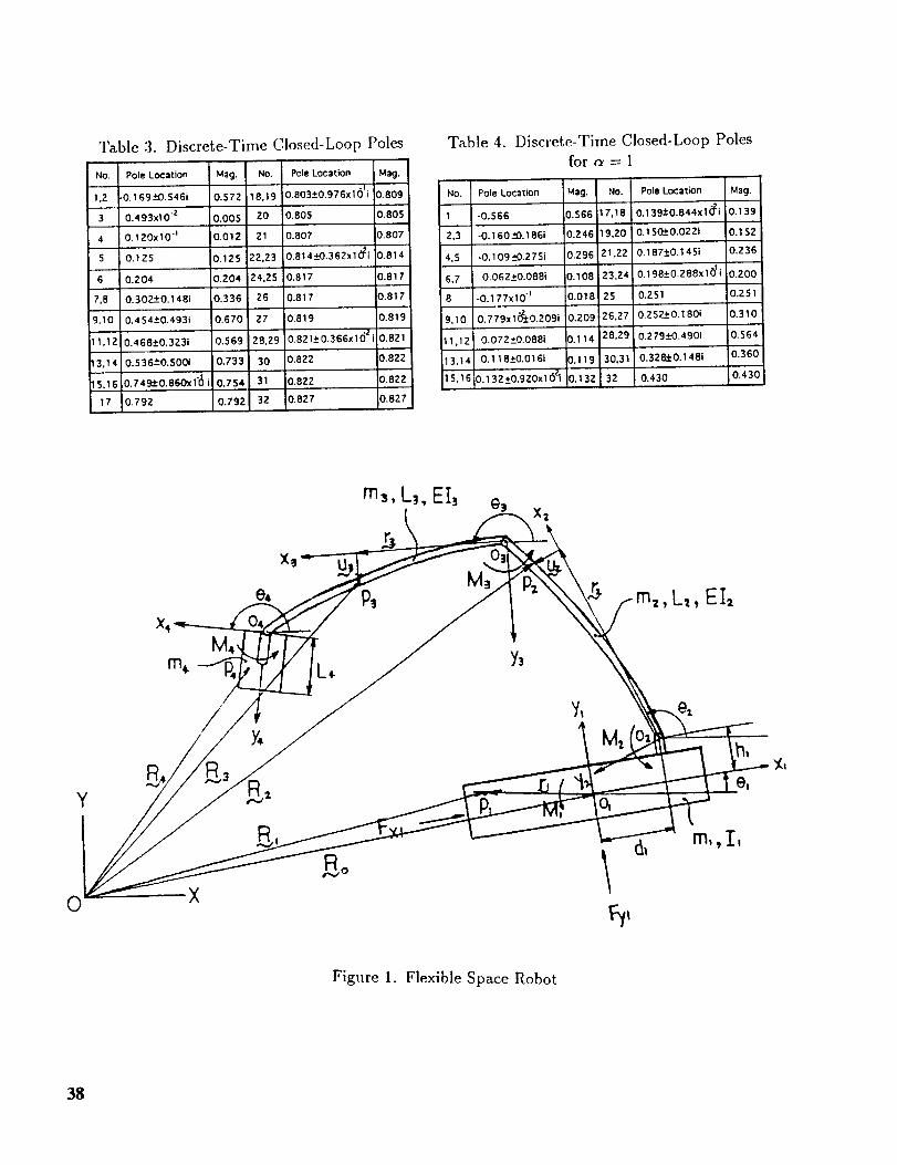
Table 3. Discrete-Time Closed-Loop Poles
NO,
1,2
3
4
5
6
7,8
9,10
11,12
13,14
15,16
17
Pole Location M_g. No. Pole Location Mag.
•O. 169:b0.$46i 0.572 18,19 0,803 -+O.976x16_i 0.809
0.493xlo "z 0.005 i 20 0.805 0.805
O. 12OxlO "1 O.012 21 0.807 L807
0.t25 0.125 22,23 0.814- -+0.382x10²i ).814
0.204 0.204 24,25 0.817 ).817
0.302-_0.1481 0.336 26 0.817 0.817
0.454_+0.493t 0.670 27 0.819 0.819
0.468+O.323i 0.569 28,29 I0.821- +0.366xldz 0.821
0.536_+0.5001 0.733 30 0.822 0.822
0.749d:O.860x1"_ i 0.754 31 0.822 3.822
0.792 0.792 32 0,827 _}.827
Table 4. Discrete-Time Closed-Loop Poles
fora=l
No. Pole Location Mag. No. Pole Location Mag.
1 -O.566 i0.$66 17,18 0.139+O.844x1_Zi 0.139
2.3 -0.160:t_).186i 0.246 i19,20 0,150:!:0.022i 0.152
4,5 -0.109-+0.275i 0.296 21,22 0.187+0.145i 0.236
6.7 0.062-+0-088i ).108 23,24 0.198-+0-288 xl{)_i 0.200
8 -0.177x10 "1 0.018 25 0.251 0.251
9,10 O.779xl(_'J:O.209i 0.209,26,27 0.252_.0.180i 0.310
11.12 0.072+0.088i 0.114 28,29 0.279_+0.490i i0.564
13.141 0.118_+0.016i 0119 30,31 0.328.'t:0.1481 0.360
15,16_0.132÷0.920x1_1 0.132 32 0.430 0.430
Y
0 X
, L2,
ml,ll
Figure 1. Flexible Space Robot
38

u_ B3
platform
Figure 2. Definition of Body Axes
x 3
zz
E
t /w'- "i,'
20 !q' Mz°
/ Mlo
1o I ;- M,o
I", _ / M,o
o ',-1
-2o
-3o
_ jf
%:,_% /
I f f
1 2 3
Ume [,1
Figure 3. Zero-Order Forces and Torque8
Figure 4b. LQR-Controiled Maneuver
0.2
_' -0.2
-0.3
O
-o.4u
O. 1 s'N
-0. I -._,_ "., ..,-_
__." x,t(2) _-_.,__.
-0.8-0.5 XpI(1)
-0.7
-0.8 f i z0 1 2 3
Figure 5.
Um_['l
Uncontrolled End-Effector
Position Errors
39

0.03
0.025
0.02
0.015
_' o.ol
0.005
_ oII
-0.005
-0.01
-0.015
-0.020
xpl(2) ,,_
I i
! 2
time Is]
Figure 6. LQR-Controlled End-Effector
Position Errors for a = 0.1
O
XI0-3
5
4
3 xPdl)
2
x,,c3) _£,,-!
-2 i t0 ! 2
Ume [s]
Figure 7. LQR-Controlled End-EffecLor
Position Errors for a = 1
4O


![II N94-33493 - NASA · ii n94-33493 high performance jet-engine flight ... w nch instruments & transmitter] ... 1171. flight ensemble averaging](https://cdn.vdocuments.us/doc/165x107/5bc3cd6509d3f299608d70f1/ii-n94-33493-nasa-ii-n94-33493-high-performance-jet-engine-flight-w-nch.jpg)