
Munich Personal RePEc Archive
Estimating ordered categorical variables
using panel data: a generalized ordered
probit model with an autofit procedure
Pfarr, Christian and Schmid, Andreas and Schneider, Udo
University of Bayreuth
10 June 2010
Online at https://mpra.ub.uni-muenchen.de/23203/
MPRA Paper No. 23203, posted 11 Jun 2010 00:55 UTC

1
Universität Bayreuth
Rechts- und Wirtschaftswissenschaftliche Fakultät
Wirtschaftswissenschaftliche Diskussionspapiere
Estimating ordered categorical variables using panel data: a
generalized ordered probit model with an autofit procedure
Christian Pfarr – Andreas Schmid – Udo Schneider
Discussion Paper 02-10
June 2010
ISSN 1611-3837
Correspondence address:
University of Bayreuth
Department of Law and Economics
Institute of Public Finance
D-95447 Bayreuth
Phone: +49-921-554324
Email: [email protected]

2
Abstract:
Estimation procedures for ordered categories usually assume that the estimated coefficients
of independent variables do not vary between the categories (parallel-lines assumption). This
view neglects possible heterogeneous effects of some explaining factors. This paper describes
the use of an autofit option for identifying variables that meet the parallel-lines assumption
when estimating a random effects generalized ordered probit model. We combine the test
procedure developed by Richard Williams (gologit2) with the random effects estimation
command regoprob by Stefan Boes.
JEL: C23; C25; C87; I10
Keywords: generalized ordered probit; panel data; autofit, self-assessed health
Citation of the software module:
regoprob2 is not an official Stata command. It is a free contribution to the research commu-
nity – like a paper – and available on SSC archive. Please cite it as such.
Pfarr, C., Schmid, A. and U. Schneider (2010), REGOPROB2: Stata module to estimate ran-
dom effects generalized ordered probit models (update), Statistical Software Components,
Boston College Department of Economics.

3
1 Introduction
When estimating a model for ordered categorical variables, normally, one faces an all-or-
nothing situation. On the one hand, estimation procedures for ordered categories usually
assume that the estimated coefficients of independent variables do not vary between the cat-
egories (parallel-lines assumption, cf. Long (1997)). This view neglects possible heterogene-
ous effects of some explaining factors. For example, the traditional ordered probit model im-
plies that all variables are constraint and meet the parallel-lines assumption. On the other
hand, a fully flexible approach (generalized ordered probit) allows all coefficients to vary
across the categories, which again is a very strong assumption. Of course, manually setting
only some variables as constrained would be an option. However, in most cases theory does
not provide adequate guidance to determine those variables that do not vary. Thus, a prag-
matic and empirically robust approach is wanted.
In contrast to cross-section data for which the procedure gologit2 (cf. Williams (2006)) pro-
vides an automated selection mechanism, up to now, such an instrument was not available
for panel data. Regoprob2, the stata module proposed in this paper, presents a solution to
this problem. It is a user-written program and an extension of regoprob that estimates ran-
dom effects generalized ordered probit models for ordinal dependent variables. It includes an
optional automated fitting procedure for identifying the relevant variables that meet the pa-
rallel-lines assumption (cf. Pfarr, Schmid and Schneider (2010)).
In the following we give a brief introduction to the theoretic background and illustrate the
application and the benefits of regoprob2 using an estimation of self assessed health.
2 Framework
When analyzing ordered choice models, the presence or absence of individual heterogeneity
is highly relevant. For instance, considering homogenous groups like “fruit flies” the assump-
tions of zero mean, homoscedasticity and homogenous thresholds are plausible without a
doubt. However, the analysis of a population of individuals e.g. regarding their subjective
well-being or self assessed health status might be more complicated (cf. Greene and Hensher
(2010), p. 208). The regression equation of an ordered categorical variable such as self as-
sessed health (SAH) will include socio-economic variables like income, education, marital
status or health related variables as well as a series of measurable and immeasurable factors
affecting the decision to choose one of the health categories. This raises the question if a zero
mean and homoscedastic errors can be presumed and if so, whether these assumptions can
capture the existing heterogeneity adequately. Hence, the hypothesis of equal thresholds for
all individuals is at least questionable (Greene and Hensher (2010)).

4
More formally, consider the observed categorical variable self assessed health with an under-
lying latent health status of the respondent y*. In this case, ordered response models are the
basic standard estimation procedure. Following the work of Boes and Winkelmann (2006)
and focusing on the cross-section case first, let y be the ordered categorical outcome, y {1,
2,…, J} where J denotes the number of distinct categories. The cumulative probabilities of the
discrete outcome are then related to a set of explanatory variables x:
Pr | 1, ,j
y j x F x j J (1.1)
Here, ĸj are the unknown threshold parameters and βs are the unknown coefficients.1 The
function F usually represents a cumulative standard normal or logistic distribution, resulting
in an ordered probit model or an ordered logit model respectively. Including the underlying
latent variable, this results in:
*1if and only if 1, ,
j jy j y x u j J (1.2)
This means that the thresholds divide the linear slope (y*) into J categories. Moreover, ob-
servable and unobservable factors influence the latent variable health. For the latter factors, a
zero mean and a constant variance is assumed, e.g. σ2 = 1 for the ordered probit model.
The probability that a respondent reports his health status to be in category j can then be
written as:
1Pr |j j
y j x F x F x (1.3)
For identification purposes, it is necessary to set the constant of the regression to zero and to
assume a constant variance.
However, one obstacle to the appropriate implementation of an ordered probit model is the
single index or parallel-lines assumption (Long (1997)). In traditional models for categorical
dependent variables the coefficient vector β is assumed to be the same for all categories J.
This means that with the increase of an independent variable, the cumulated distribution
shifts to the right or left but there is no shift in the slope of the distribution. Boes and Win-
kelmann (2006), Greene, Harris, Hollingsworth et al. (2008) and Pudney and Shields (2000)
suggest that in the set of thresholds, individual variation is an indicator for heterogeneity that
appears in the data and that this case is not reflected in traditional ordered probit models.
Relaxing the assumption of equal thresholds for all individuals and allowing the indices to
1 One assumption on the threshold parameters is that 1,i ij and that J and o .

5
differ across the outcomes leads to a generalized ordered probit model. Here, the threshold
parameters depend on the covariates:
,j j j
x (1.4)
where γj are the influence parameters of the covariates on the thresholds. Entering the thre-
shold equation (1.4) into the cumulative probability of the generalized ordered probit model
leads to the following expression:
Pr | 1, ,j j j j
y j x F x x F x j J (1.5)
As one can see from equation (1.5), the coefficients of the covariates and the threshold coeffi-
cients cannot be identified separately when the same set of variables x is used. It follows that
j j and that the generalized ordered probit model has one index ´
jx for each cate-
gory j of the outcome variable.2 This approach leads to the estimation of J-1 binary probit
models (Williams (2006)). The first model estimates category 1 versus categories 2,…, J; the
second model does the same regarding categories 1 and 2 versus 3,..., J. Equation J-1 then
compares the choice between categories 1,…, J-1 versus category J. This specification allows
for individual heterogeneity in the β-parameters that leads to heterogeneity across the cate-
gories of the dependent variable.
For panel data, individual heterogeneity is accounted for using a random effects generalized
ordered probit approach (cf. Boes (2007), p. 133). More formally, let SAH be an ordinal vari-
able which takes on the values j = 1,…, J. In contrast to the cross-section representation, the
outcome probabilities are conditional on the individual effect i :3
'1
' '1
'1
Pr 1| ,
Pr | , 2, , 1
Pr | , 1
it it i it i
it it i it y i it y i
it it i it J i
Y x F x
Y j x F x F x j J
Y J x F x
(1.6)
For the individual effects, a zero mean and a constant variance σ2 is assumed so that
² / (1 ²) . As for the cross-section version of the generalized ordered probit model, the
approach allows any number of the βy (from none to all) to vary across the categories.
Hence, using panel data allows for the inclusion of two kinds of heterogeneity. First, unob-
served individual heterogeneity is captured by a random effects specification. Second, differ-
2 The generalized ordered probit model nests the standard ordered probit model with the restriction that
1 1...J
.
3 Note that in equation (1.6) the beta coefficients differ between the categories of the dependent varia-ble.

6
ences in the cut-points and therefore in the beta coefficients represent the observed hetero-
geneity in the reporting of the categorical variable.
However, the problem of identifying the constrained variables remains unsolved. As pointed
out above, theory often does not provide good guidance. As both extremes – setting all or
none variables constrained are equally unlikely, a pragmatic and empirically robust approach
is wanted. Building on the automated fitting procedure that Williams (2006) developed for
gologit2 we suggest an iterative fitting process that we have implemented in regoprob2. The
autofit option of regoprob2 triggers an iterative process used to identify the random effects
generalized ordered probit model that best fits the data.
At the beginning, an unconstrained model (all coefficients could vary) is estimated. Then, in a
first step, a Wald test is applied on each variable to prove whether the coefficients differ
across equations. The least significant variable is then set as constrained, that means to have
equal effects over all categories. With autofit2(alpha) one can choose another significance
level than the standard one. The parameter alpha is the desired significance level for the
tests; alpha must be greater than 0 and less than 1. If autofit is specified without parameters,
as in this case, the default alpha-value is .05. Note that the higher alpha is, the easier it is to
reject the parallel lines assumption, and the less parsimonious the model will tend to be.4
Then the model is refitted with the constraints identified so far and the step is repeated until
only significant variables remain. Finally, as specification test, a global Wald test on the full
model with constraints is applied to confirm the null hypothesis that the parallel-lines as-
sumption is not violated. The following example illustrates the process and describes the fit-
ting procedure in more detail.
3 Estimating a generalized ordered probit model with the autofit option:
an example
To discuss the estimation of a random effects generalized ordered probit model for ordered
categorical variables we use self assessed health as dependent variable. It is a 5-point categor-
ical variable with 1 indicating very bad and 5 very good self reported health status. As expla-
natory variables, a set of ten dummy variables indicating various diseases is used.5 For illu-
stration purposes, we restrict the analysis to a 10 %-random sample of the original SAVE da-
ta6 consisting of 1,186 individuals for the years 2006 to 2008.
4 This option may be time consuming depending on the sample size and the number of explanatory variables. 5 For more details regarding reporting heterogeneity in self-assessed health see Pfarr, Schneider, Schneider et al. (2010). 6 The SAVE study is conducted by the Mannheim Research Institute for the Economics of Aging (MEA) and was started in 2001. Originally, the longitudinal study on households’ financial behavior focused

7
Table 1: Variable description
variable name label
health self assessed health, 1=very bad, 5=very good
backache 1, if chronic backache
blood 1, if individual suffer from hypertension
cancer 1, if individual is diagnosed with cancer
chol 1, if individual has a higher cholesterol level
gastric_ulcer 1, if a gastric ulcer is diagnosed
heart 1, if individual suffers heart diseases
mental 1, if mental disorders
other_disease 1, if other diseases
pul_asthma 1, if chronic chest disease or asthma
stroke 1, if circulatory disorders or stroke
First, we start with a fully constraint model (random effects ordered probit) (cf. Frechette
(2001)). As it is clear from the results presented below (see figure 1), with the exception of
gastric_ulcer, all other disease variables show the expected significant negative sign. The
magnitude of the partial effects varies between the variables.
Figure 1: Results of the fully constrained random effects ordered probit model.
on savings and old-age provisions but also deals with aspects of health and health behavior (cf. Börsch-Supan, Coppola, Essig et al. (2008)).

8
In contrast to the results above, a generalized ordered probit model allows different parame-
ter vectors for each outcome. This means that we aim at assessing the observable individual
heterogeneity in the threshold parameters as well as in the mean of the regression (cf. Greene
and Hensher (2010)). From figure 2, it is obvious that the magnitude of the coefficients as
well as the level of significance vary between the four binary probit models. The coefficients
of backache are significant throughout the equations and range from -0.66 to -1.52. While the
ordered probit estimation shows a highly significant impact, the generalized model also im-
plies an increasing significant negative coefficient. This means that individuals suffering from
chronic backache are less likely to report a better health status. The effect is lower when
comparing SAH categories 1 vs. 2-5, and highest for categories 1-4 vs. 5. For the variable
blood, only equations 3 and 4 show a significant impact. People with hypertension tend to
report the extreme categories of SAH less often. In consequence, those individuals will
choose the middle categories more often. For heart diseases, it is obvious that there exists a
tendency to assign oneself into the lowest categories of SAH.
If one looks at the overall significance reported by a likelihood ratio test, the generalized or-
dered probit model fails to reject the hypothesis that all coefficients have no influence. Con-
sequently, a model with full variation seems to be overspecified and therefore unsuitable for
estimating ordered categorical models.
Figure 2: Random effects generalized ordered probit with all variables varying.

9
Thus, at this point, it has to be decided, which variables are most likely constrained and
which should be allowed to vary. To the best knowledge of the authors, there is no good
theory that would reliably predict if a certain illness presents a constrained or an uncon-
strained factor regarding SAH – a typical problem encountered in many similar cases. For
this reason, we now apply the autofit procedure as suggested above.7
In our example, the first step in the estimation process is a model with full variation of all ten
explanatory variables. After estimation of this model and Wald tests on each coefficient, the
variable mental with a P-value of 0.9437 is identified as the least significant variable after the
first step. Next, this procedure is repeated with the variable mental set as constraint. In step
two, gastric_ulcer meets the parallel-lines assumption.
Figure 3: An example of the autofit procedure.
7 For a more detailed discussion of the autofitting procedure see Williams, R. (2006) and for the theo-retical background of estimating random effects generalized ordered probit models see Boes, S. (2007).
10
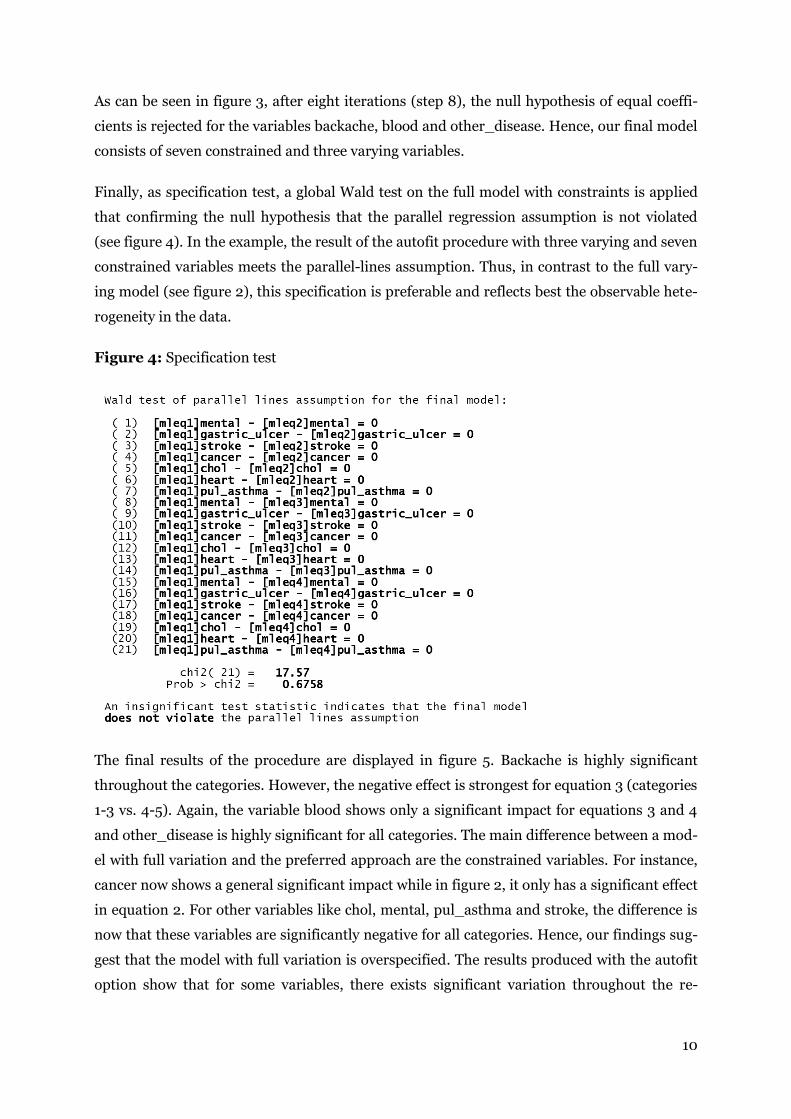
As can be seen in figure 3, after eight iterations (step 8), the null hypothesis of equal coeffi-
cients is rejected for the variables backache, blood and other_disease. Hence, our final model
consists of seven constrained and three varying variables.
Finally, as specification test, a global Wald test on the full model with constraints is applied
that confirming the null hypothesis that the parallel regression assumption is not violated
(see figure 4). In the example, the result of the autofit procedure with three varying and seven
constrained variables meets the parallel-lines assumption. Thus, in contrast to the full vary-
ing model (see figure 2), this specification is preferable and reflects best the observable hete-
rogeneity in the data.
Figure 4: Specification test
The final results of the procedure are displayed in figure 5. Backache is highly significant
throughout the categories. However, the negative effect is strongest for equation 3 (categories
1-3 vs. 4-5). Again, the variable blood shows only a significant impact for equations 3 and 4
and other_disease is highly significant for all categories. The main difference between a mod-
el with full variation and the preferred approach are the constrained variables. For instance,
cancer now shows a general significant impact while in figure 2, it only has a significant effect
in equation 2. For other variables like chol, mental, pul_asthma and stroke, the difference is
now that these variables are significantly negative for all categories. Hence, our findings sug-
gest that the model with full variation is overspecified. The results produced with the autofit
option show that for some variables, there exists significant variation throughout the re-

11
ported categories. To sum up, the three variables blood, backache and other_disease drive
the observed heterogeneity in our dependent variable self-assessed health.
Figure 5: Regoprob2 with autofit

12
4 Conclusion
In the empirical analysis of categorical dependent variables, the problems associated with the
parallel-lines assumption should be taken into account. To deal with this, knowledge about
the effects of the explanatory variables on the different categories is needed. An analysis
based on an underlying theory, that provides information about the variables that violate the
parallel-lines assumption would be preferable. But in most cases that is not the case. With the
autofitting procedure implemented in regoprob2, we suggest a pragmatic and empirically
robust approach to identify the variables that should be constrained. Furthermore, to the best
knowledge of the authors, this is the first application of this kind for panel data. Taking into
account that a standard ordered probit model may violate the parallel-lines assumption and
that a full-variation model is often overspecified, in absence of theory based advice an itera-
tive procedure like autofit could be seen as the “lesser of three evils”. In our example, we
show in how far a variable such as self-assessed health is prone to observed heterogeneity. If
one does not account for this, any varying effects of the explanatory variables on the catego-
ries will be neglected in the standard ordered probit model. Accordingly, our regoprob2
command combines the detection of observed heterogeneity in categorical variables with the
inclusion of unobserved individual heterogeneity using a fixed effects estimator.
5 Acknowledgements
Stefan Boes of the University of Zurich wrote regoprob and kindly gave permission to use
parts of his code for regoprob2. See regoprob for a description of the former regoprob com-
mand.
Richard Williams of the Notre Dame Department of Sociology wrote gologit2 and kindly gave
permission to use parts of his code for programming goprobit. For a more detailed descrip-
tion of gologit2 and its features, see the reference below or gologit2.
6 References Boes, S. (2007), Three Essays on the Econometric Analysis of Discrete Dependent Variables,
Universität Zürich, Zürich.
Boes, S. and Winkelmann, R. (2006), Ordered Response Models, in: Allgemeines Statisti-sches Archiv, 90, pp. 167–181.
Börsch-Supan, A., Coppola, M., Essig, L., Eymann, A. and Schunk, D. (2008), The German SAVE Study - Design and Results, mea studies 06, Mannheim Research Institute for the Economics of Aging, Mannheim.
Frechette, G. R. (2001), sg158: Random-Effects Ordered Probit, in: Stata Technical Bulletin, 59, pp. 23–27.

13
Greene, W. H., Harris, M. N., Hollingsworth, B. and Maitra, P. (2008), A Bivariate Latent Class Correlated Generalized Ordered Probit Model with an Application to Mod-eling Observed Obesity Levels, Working Paper, Nr. 08-18, New York University, Department of Economics, New York.
Greene, W. H. and Hensher, D. A. (2010), Modeling ordered choices, A primer, Cambridge University Press, Cambridge.
Long, J. S. (1997), Regression models for categorical and limited dependent variables, Sage Publ., Thousand Oaks, Calif.
Pfarr, C., Schmid, A. and Schneider, U. (2010), REGOPROB2: Stata module to estimate ran-dom effects generalized ordered probit models (update), Statistical Software Components, Boston College Department of Economics.
Pfarr, C., Schneider, B. S., Schneider, U. and Ulrich, V. (2010), Self-assessed health, gender differences and reporting heterogeneity: empirical evidence using multiple im-puted data, Discussion Paper, Nr. 03-10, University of Bayreuth, Department of Law and Economics, Bayreuth.
Pudney, S. and Shields, M. (2000), Gender, Race, Pay and Promotion in the British Nursing Profession, Estimation of a Generalized Ordered Probit Model, in: Journal of Ap-plied Econometrics, 15(4), pp. 367–399.
Williams, R. (2006), Generalized ordered logit/partial proportional odss models for ordinal dependent variables, in: Stata Journal, 6(1), pp. 58–82.

Universität Bayreuth
Rechts- und Wirtschaftswissenschaftliche Fakultät
Wirtschaftswissenschaftliche Diskussionspapiere
Zuletzt erschienene Papiere:*
01-10 Herz, Bernhard Wagner, Marco
Multilateralism versus Regionalism!?
05-09 Erler, Alexander Krizanac, Damir
Taylor-Regel und Subprime-Krise – Eine empirische Analyse der US-amerikanischen Geldpolitik
04-09 Woratschek, Herbert Schafmeister, Guido Schymetzki, Florian
International Ranking of Sport Management Journals
03-09 Schneider Udo Zerth, Jürgen
Should I stay or should I go? On the relation between primary and secondary prevention
02-09 Pfarr, Christian Schneider Udo
Angebotsinduzierung und Mitnahmeeffekt im Rahmen der Riester-Rente. Eine empirische Analyse.
01-09 Schneider, Brit Schneider Udo
Willing to be healthy? On the health effects of smoking, drinking and an unbalanced diet. A multivariate probit approach
03-08 Mookherjee, Dilip Napel, Stefan Ray, Debraj
Aspirations, Segregation and Occupational Choice
02-08 Schneider, Udo Zerth, Jürgen
Improving Prevention Compliance through Appropriate Incentives
01-08 Woratschek, Herbert Brehm, Patrick Kunz, Reinhard
International Marketing of the German Football Bundesliga - Exporting a National Sport League to China
06-07 Bauer, Christian Herz, Bernhard
Does it Pay to Defend? - The Dynamics of Financial Crises
05-07 Woratschek, Herbert Horbel, Chris Popp, Bastian Roth, Stefan
A Videographic Analysis of "Weird Guys": What Do Relationships Mean to Football Fans?
04-07 Schneider, Udo Demographie, Staatsfinanzen und die Systeme der Sozialen Sicherung
03-07 Woratschek, Herbert Schafmeister, Guido
The Export of National Sport Leagues
02-07 Woratschek, Herbert Hannich, Frank M. Ritchie, Brent
Motivations of Sports Tourists - An Empirical Analysis in Several European Rock Climbing Regions
* Weitere Diskussionspapiere finden Sie unter http://www.fiwi.uni-bayreuth.de/de/research/Working_Paper_Series/index.html


