
MPRAMunich Personal RePEc Archive
The Wear and Tear on Health: What isthe Role of Occupation?
Bastian Ravesteijn and Hans van Kippersluis and Eddy van
Doorslaer
Erasmus University Rotterdam, Tinbergen Institute
18. September 2013
Online at http://mpra.ub.uni-muenchen.de/50321/MPRA Paper No. 50321, posted 2. October 2013 18:32 UTC

Bastian Ravesteijn, Hans van Kippersluis and Eddy van Doorslaer The Wear and Tear on Health What is the Role of Occupation?
DP 09/2013-028

The Wear and Tear on Health: What Is the Role
of Occupation?
Bastian Ravesteijn, Hans van Kippersluis, Eddy van Doorslaer∗
September 14, 2013
Abstract
While it seems evident that occupations affect health, effect estimates are
scarce. We use a job characteristics matrix in order to characterize occu-
pations by their physical and psychosocial burden in German panel data
spanning 26 years. Employing a dynamic model to control for factors that
simultaneously affect health and selection into occupation, we find that
manual work and low job control both have a substantial negative effect
on health that increases with age. The effects of late career exposure to
high physical demands and low control at work are comparable to health
deterioration due to aging by 16 and 23 months respectively.
Average health and life expectancy differ substantially across occupational groups
(Marmot et al., 1991; Case and Deaton, 2005). For example, manual workers
∗Ravesteijn: Department of Economics, Erasmus University Rotterdam, P.O. Box 1738,3000 DR Rotterdam, Netherlands (e-mail: [email protected]); Van Kippersluis: Departmentof Economics, Erasmus University Rotterdam, P.O. Box 1738, 3000 DR Rotterdam, Nether-lands (e-mail: [email protected]); Van Doorslaer: Department of Economics, Eras-mus University Rotterdam, P.O. Box 1738, 3000 DR Rotterdam, Netherlands (e-mail: [email protected]). This paper derives from the NETSPAR funded project “Income, healthand work across the life cycle II” and was supported by the National Institute on Aging of theNational Institutes of Health under Award Number R01AG037398. We thank Alberto Abadie,Andrew Jones, Anne Gielen, Arthur van Soest, Bas van der Klaauw, Erzo Luttmer, JeffreyWooldridge, Maarten Lindeboom, Owen O’Donnell, Rainer Winkelmann, Stephane Bonhomme,and seminar participants at Tilburg University, Erasmus University Rotterdam, the PhD Semi-nar on Health Economics and Policy in Grindelwald, the Netspar international pension workshopin Frankfurt, the conference of the International Health Economics Association in Sydney, andthe Congress of the European Economic Association for helpful comments. Errors are our own.
1

in the US are 50 percent more likely to die within a given year than workers
in managerial, professional and executive occupations (Cutler et al., 2008). In
eight European countries, the mortality rate for manual workers is higher than
for nonmanual workers throughout the age distribution (Mackenbach et al., 1997;
Kunst et al., 1998), and this gap has widened over time (Mackenbach et al., 2003).
For the Netherlands, Ravesteijn et al. (2013) find a strong gradient in self-assessed
health by occupational class, especially at an older age, and note that at the age
of 60, 20 percent of elementary workers have exited the workforce into disability,
as opposed to 8 percent among workers in occupations that require academic
training.
Apart from occupation exerting a causal effect on health, this strong correla-
tion between occupation and health could also stem from reverse causality, with
health constraining occupational choice. Moreover, individuals in different occu-
pational groups can differ in other observed and unobserved ”third factors” that
potentially influence health. For example, manual workers may have lower educa-
tion, or they may have a different genetic predisposition. Both reverse causality
and third factors may lead to selection effects: people with good health prospects
are selected into certain types of occupation, and as a result the size of the asso-
ciation may be very different from the size of the causal effect of occupation on
health.
In this paper we aim to assess the extent to which the observed association
is due to causation from occupation to health. This is important from a fairness
perspective, as well as from a productivity perspective. From a fairness perspec-
tive, health disparities that result from occupational stressors may be socially
undesirable. Policymakers may want to distinguish between health disparities
resulting from free choice behavior, such as smoking or drinking, and from occu-
pational stressors that can only be chosen from a heavily constrained choice set.
From a productivity perspective, policymakers and employers are interested to
know which specific occupational characteristics are most harmful to health. For
example, occupations with harmful ergonomic workplace conditions may simul-
taneously be characterized by low control possibilities at work, which may exert
an independent effect on health. Consequently, improved knowledge about these
separated effects will allow for better-targeted efforts in order to reduce sickness
2

absenteeism and disability through adjustment of specific labor conditions.
Many studies have documented strong associations between type of occupation
and health (see e.g. Kunst et al., 1999; Goodman, 1999). Only very few attempt
to obtain estimates of a causal effect and those that do often focus on very specific
occupations or specific exposure to health-harming circumstances (e.g. Bongers
et al., 1990, who study back pain among helicopter pilots). In the economic
literature the relationship between occupation and health has received surprisingly
little attention, yet interest has been growing in recent years. Case and Deaton
(2005) show that the self-reported health of manual workers is lower and declines
more rapidly with age than of nonmanual workers. Choo and Denny (2006) report
similar patterns for Canadian workers while controlling for a more extensive set
of lifestyle factors, and suggest that manual work has an independent effect on
health over and above any differences in lifestyle across occupations. Using the
longitudinal Panel Study of Income Dynamics (PSID), Morefield et al. (2012)
estimate that five years of blue collar employment predicts a four to five percent
increase in the probability of moving from good to bad health. Yet, as the authors
acknowledge, these studies are limited in their ability to investigate the role of
factors that may affect both selection into certain types of occupation and health
itself.1
Using a three-digit occupational classification, Fletcher et al. (2011) combine
the information on physical requirements of work and environmental conditions
taken from the Dictionary of Occupational Titles (DOT) with occupational in-
formation in the US Panel Study of Income Dynamics (PSID). Their aim is to
estimate the health impact of five year exposure to these physical and environmen-
tal conditions. They include first-observed health and five-period lagged health in
their model and they find negative effects of physical demands and environmental
1Apart from current occupation, workers’ entire occupational history is likely to have animpact on current health. Fletcher and Sindelar (2009) use father’s occupation during child-hood and the proportion of blue collar workers in the state as instrumental variables for firstoccupation, and find that first occupation in a blue collar occupation has a negative effect onself-assessed health. Kelly et al. (2011) question the statistical relevance of the two instrumen-tal variables used in Fletcher and Sindelar (2009), and instead propose methods developed byLewbel (2012) and Altonji et al. (2005) in order to investigate the causal effect of first occu-pation on health. They find that entering the labor market as a blue collar worker raises theprobabilities of obesity and smoking, by 4 and 3 percent respectively. This indicates that theeffect of occupation on health may – at least partly – be transmitted through lifestyles.
3
conditions on health for women and older workers but not for men and nonwhite
women, and strong negative effects of environmental conditions for young men but
not for young women. Fletcher et al. (2011) acknowledge that the potential endo-
geneity of occupation and occupational change does not allow their random effects
estimates to have a causal interpretation. Reverse causality and unobserved third
factors may lead to biased estimators, and in their approach it is impossible to
disentangle the contributions of physical and psychosocial occupational stressors.
In this study, we aim to overcome these limitations in two ways. First, we esti-
mate a fixed effects model that controls for lagged health in order to estimate the
effect of exposure to occupational stressors in the previous year on current health.
From a theoretical model of occupation and health over the life cycle, we derive
health-related selection mechanisms into occupation, show how our econometric
estimators relate to the structural parameters, and explicitly formulate conditions
under which our estimates have a causal interpretation. We argue that, in the
absence of exogenous variation in the regressor(s) of interest, but with panel data
spanning 26 years, our model offers the most trustworthy causal estimates. Our
alternative formulation of the Grossman (1972) model illustrates its implicit as-
sumptions on the decaying effect of past shocks and health investment on current
health. These insights are informative for anyone trying to provide theoretical
foundations for an econometric dynamic panel data model.
Second, we argue that manual occupations are not only more physically de-
manding, but are simultaneously often characterized by low psychosocial work-
load. In previous research, most existing studies have characterized occupation
with a binary indicator of manual versus nonmanual occupation, or have focused
only on the manual aspects of occupation. This made it impossible to disentan-
gle the contributions of the different ergonomic and psychosocial stressors, which
meant that the resulting policy implications were unclear. In the present study,
we link detailed Finnish data on occupational stressors to individual-level German
longitudinal data. This provides a level of detail that was not available in earlier
studies. The US DOT, for example, lacks information on psychosocial workplace
conditions and exclusively includes information on physical requirements and en-
vironmental conditions.
Our findings suggest that about 50 percent of the association between physical
4
demands at work and self-reported health is due to the causal effect of physical
demands. Selection accounts for the remaining 50 percent. The average immediate
effect of a one standard deviation increase in the degree of manually handling
heavy burdens (e.g. from a wholesale worker to a plumber or from a mail sorter
to a bricklayer) is comparable to the effect of aging five months and the effect
increases with age. A lower degree of control over daily activities at work (e.g.
kitchen assistant instead of cook or nurse instead of physiotherapist) is harmful to
health at older, but not at younger ages. Under the assumption that the coefficient
of lagged health captures the decay rate of past choices and shocks, we estimate
that exposure to a one standard deviation increase in handling heavy burdens
between age 60 to 64 leads to a health deterioration that is comparable to aging
16 months. The estimated effect of exposure to low job control between age 60 to
64 is comparable to aging 23 months.
The paper is organized as follows: Section I discusses the theoretical relation-
ship between occupation and health. Section II introduces the German Socioeco-
nomic Panel. Section III outlines our empirical approach to estimating the effect
of manual work on health. Section IV presents the results. Section V discusses
how our results relate to the literature and concludes.
1 Occupation and health over the life cycle
In the economics literature, health is treated as a durable capital stock which
depreciates with age and can be increased by investment (Grossman, 1972). The
age-related health depreciation rate is exogenous, but an individual can invest in
his health through the purchase of (preventive or curative) medical care. The
effect of behavior on health can be positive or negative. Occupational choice can
be seen as a form of health disinvestment/erosion: an individual chooses an occu-
pation that is characterized by a set of potentially harmful occupational stressors
(Case and Deaton, 2005; Galama and van Kippersluis, 2010). Occupations with
more harmful characteristics may yield higher earnings than other, less harmful
occupations in the choice set of the individual. This difference in earnings is
known as the compensating wage differential (Smith, 1974; Viscusi, 1978). The
additional earnings may be used in order to partially offset the detrimental effect
5

of work on health by investing in health, but this is not necessarily the case, for
example when the individual spends the additional income on consumption. This
economic paradigm proves useful in detecting sources of health-related selection
into occupation.
These insights are embedded in a theoretical model of an individual maximiz-
ing the expected present value of lifetime utility, which is derived from consump-
tion c and health h, by choosing levels of consumption c, occupational stressors in
vector o, and health investment m. Each occupation is characterized by physical
and psychosocial occupational stressors which tend to be clustered, i.e. occupa-
tions with low psychosocial workload are often simultaneously characterized by
high physical demands. Future utility is discounted at discount rate β. The in-
formation set I includes endowments e and permanent health hp, all state and
choice variables up to time t, all future values of the aging rate, but not future
unforeseen health shocks η.
max{ct+j ,ot+j ,mt+j}T−tj=0E[∑T−t
j=0βju(ct+j, ht+j)|It
](1)
The health production function depends on (i) characteristics and circumstances
that remain constant over time, embodied by permanent health hp = f(e), which
is a function of endowments and reflects all circumstances and personal charac-
teristics that remain constant over the life cycle, (ii) foreseen health deterioration
because of aging a, (iii) a vector of occupational characteristics o, (iv) medical
investment m, and (v) exogenous health shocks η. The effect of occupational
characteristics on health, γo, is nonpositive, and 0 ≤ θ ≤ 1, reflects diminishing
marginal benefits to health investment. Total lifetime T is exogenous and known
to the individual and the effects of occupational stressors, health investments and
shocks are assumed to decay at the same rate φ, which lies between 0 and 1.
ht+j =hp +∑t+j
k=2
(ak + φt+j−k(γ ′ook−1 + γmm
θk−1 + ηk)
)(2)
Expenditures on consumption and health investment, at prices pc and pm respec-
tively, should not exceed the net value of wage earnings. The individual can lend
and borrow at real interest rate r, but he has to repay any remaining debt at
the end of his life. Wage w is a function of (i) current occupational choice o, (ii)
6

current health h, and (iii) endowments e.
s.t.∑T
k=1(pcck + pmmk) ≤
∑T
k=1(1 + r)k−1w(ok, hk; e) (3)
Consumption, health investment and occupational choice are chosen by equating
mar-ginal benefit to marginal cost. The marginal utility of consumption is equal
to the shadow price of income λ times the price of consumption.
∂ut∂ct
= λpc (4)
For each occupational attribute ol in vector o, the marginal benefit of occupational
stress is represented by the product of λ and the instantaneous wage premium.
The marginal cost includes the marginal deterioration of health in all future peri-
ods multiplied by (i) the discounted marginal utility of future health, and (ii) the
product of λ and the present value of the marginal wage returns to future health.
λ∂wt∂ot,l
= −∑T−t−1
j=1
∂ht+j∂otl
[βj∂ut+j∂ht+j
+ λ
(1
1 + r
)j∂wt+j∂ht+j
]∀l (5)
Health investment is the ‘mirror image’ of occupational choice. The marginal
benefit (the product of the marginal effect of health investment on health and
both the discounted marginal utility of health and the marginal wage returns to
health in all future periods) is equated to marginal cost (the product of the shadow
price of income and the price of medical care).
∑T−t−1
j=1
∂ht+j∂mt
[βj∂ut+j∂ht+j
+ λ
(1
1 + r
)j∂wt+j∂ht+j
]= λpm (6)
The theoretical framework shows how an individual takes into account the future
consequences of his decisions while deciding on the optimal levels of harmful oc-
cupational stressors. Three insights from the theory are particularly noteworthy.
First, both time-invariant initial endowments e, in the form of e.g. physical ability,
intelligence or taste for adventure, and time-varying factors such as health shocks
η (e.g. a car accident or a disease onset) may influence both occupational choice
and health status through (i) the marginal utility of health, (ii) the marginal wage
7
returns to health, and (iii) the shadow price of income λ. This means that workers
may select themselves into certain types of occupations depending on exogenous
factors that also influence health directly. The observed health differences across
occupational class should therefore not be interpreted as evidence of a causal effect
of occupation on health.
Second, in contrast to exogenous sources of health-related selection into oc-
cupation, such as endowments and shocks, individuals endogenously choose their
level of health investment. Health investment may be correlated with occupational
choice (i) because exogenous factors influence both, and (ii) because workers may
choose to offset occupation-related health damage by investing in health: e.g. a
bricklayer may seek physiotherapeutic treatment for his back pain or a manager
may take yoga classes in order to improve his mental well-being.
Third, the relationship between work and health may change over the life
cycle. This could occur for three reasons. First, as equation 6 illustrates, the ex-
pected wage returns on health investment decrease as the individual approaches
the retirement age, which implies that individuals have fewer incentives to off-
set occupational damage to health by medical investment.2 Second, possibly γo
changes over the lifetime, e.g. if health at older ages is more vulnerable to wear
and tear at the workplace. Third, even if the effect of hard work is equal at all
ages, the marginal effect of health repair may decrease with age such that full
repair of health is no longer feasible at older ages.3
In sum, our empirical identification strategy should (i) account for factors that
may influence selection into type of occupation and may also be related to health,
(ii) address how behavioral adjustments that affect health may coincide with
occupational choice, and (iii) accommodate the changing relationship between
occupation and health over the life cycle.
2Although a model which endogenizes length of life as a function of health could explain anincrease in medical investment at older ages.
3Our model does not incorporate real-world labor market rigidities, yet these may also preventindividuals from switching occupations at older ages to optimize their exposure to occupationalstressors.
8

2 Occupational stressors and the German So-
cioeconomic Panel
The German Socioeconomic Panel (GSOEP) started in 1984 and we use data from
the 26 subsequent annual waves. The full sample consists of 358,281 person-wave
observations. Sample sizes per wave range from 8,681 in the year 1989 to 20,912
in 2000. Respondents are followed over multiple waves but the panel is unbal-
anced since many respondents enter the sample after the year 1984 or leave the
sample before 2009. We limit our sample to respondents who are employed or
self-employed and of working age, i.e. between 16 and 65 years old. 35,258 indi-
viduals are recorded to have been working in at least one wave, 15,819 individuals
have been working in at least six waves and 6,813 in at least eleven waves.
Respondents were asked to rate satisfaction with their own health on an in-
teger scale from 0 to 10 which we will refer to as self-assessed health (SAH).
Occupational titles were coded into the International Standard Classification of
Occupations of the OECD (ISCO-88). These are 311 occupational classes that
were grouped into ten ranked major occupational groups by the OECD. On the
basis of the OECD classifications, we define white collar workers as legislators, se-
nior officials, managers, professionals, technicians, associate professionals, clerks.
We define blue collar workers as service workers and shop and market sales work-
ers, skilled agricultural and fishery workers, craft and related trades workers, plant
and machine operators, assemblers and workers in elementary occupations. This
is in line with the distinction between manual and nonmanual work of Case and
Deaton (2005). According to these definitions, we have a total of 122,419 person-
wave observations for white collar occupation and 110,783 observations for blue
collar occupation.
Figure 1 graphs age-predicted SAH for blue collar and white collar workers.
Blue collar workers on average report better health at younger ages, whereas the
opposite is true after the age of 28. Self-assessed health decreases for both blue
collar and white collar workers over most of the age range, but increases after the
age of 57. One should keep in mind, however, that these patterns only reflect the
SAH ratings of those who are employed.4 In line with Case and Deaton (2005),
4At older ages, unhealthy workers exit out of employment while healthy workers remain.
9

in the pooled sample we find the health decline associated with age to be much
steeper among blue collar than white collar workers. This is the observation that
begs the question why blue collar workers run down their health at a much faster
rate than white collar workers. Table 1 shows that the average SAH score for
Figure 1: Health for blue and white collar workers.
Predicted satisfaction with health for blue and white collar workers over the life cycle.
those who work is 7.05, and lower for blue collar workers (6.96) than for white
collar workers (7.10).5 Blue collar workers on average have less education and
earnings, are slightly younger and less likely to be female. Average education
among blue and white collar workers is 10.47 and 12.89 years, respectively. If we
disregard censoring, average net monthly labor earnings are 1,463 Euro for white
collar workers and 1,098 Euro for blue collar workers. While the dichotomization
into blue and white collar occupation represents a useful and convenient way to
study health differences across broad occupational groups, it does not allow us
to identify which aspects of occupational stressors associated with blue collar oc-
cupations matter most. In Finland, a Job Exposure Matrix (FINJEM) has been
5Health worsens from the top to the bottom of the OECD occupational ladder. 23 percentof legislators, senior officials and managers rate their health with a five or less, as opposed to 31percent of elementary workers. 49 percent of legislators, senior officials and managers rate theirhealth with at least an eight, while for elementary workers this is only 42 percent. This patternis monotonic across the nine ranked major OECD occupational groups.
10
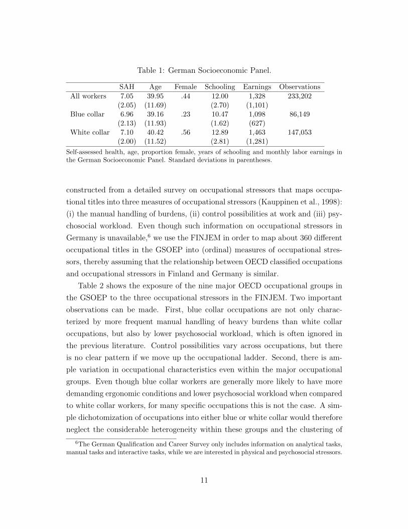
Table 1: German Socioeconomic Panel.
SAH Age Female Schooling Earnings Observations
All workers 7.05 39.95 .44 12.00 1,328 233,202(2.05) (11.69) (2.70) (1,101)
Blue collar 6.96 39.16 .23 10.47 1,098 86,149(2.13) (11.93) (1.62) (627)
White collar 7.10 40.42 .56 12.89 1,463 147,053(2.00) (11.52) (2.81) (1,281)
Self-assessed health, age, proportion female, years of schooling and monthly labor earnings inthe German Socioeconomic Panel. Standard deviations in parentheses.
constructed from a detailed survey on occupational stressors that maps occupa-
tional titles into three measures of occupational stressors (Kauppinen et al., 1998):
(i) the manual handling of burdens, (ii) control possibilities at work and (iii) psy-
chosocial workload. Even though such information on occupational stressors in
Germany is unavailable,6 we use the FINJEM in order to map about 360 different
occupational titles in the GSOEP into (ordinal) measures of occupational stres-
sors, thereby assuming that the relationship between OECD classified occupations
and occupational stressors in Finland and Germany is similar.
Table 2 shows the exposure of the nine major OECD occupational groups in
the GSOEP to the three occupational stressors in the FINJEM. Two important
observations can be made. First, blue collar occupations are not only charac-
terized by more frequent manual handling of heavy burdens than white collar
occupations, but also by lower psychosocial workload, which is often ignored in
the previous literature. Control possibilities vary across occupations, but there
is no clear pattern if we move up the occupational ladder. Second, there is am-
ple variation in occupational characteristics even within the major occupational
groups. Even though blue collar workers are generally more likely to have more
demanding ergonomic conditions and lower psychosocial workload when compared
to white collar workers, for many specific occupations this is not the case. A sim-
ple dichotomization of occupations into either blue or white collar would therefore
neglect the considerable heterogeneity within these groups and the clustering of
6The German Qualification and Career Survey only includes information on analytical tasks,manual tasks and interactive tasks, while we are interested in physical and psychosocial stressors.
11
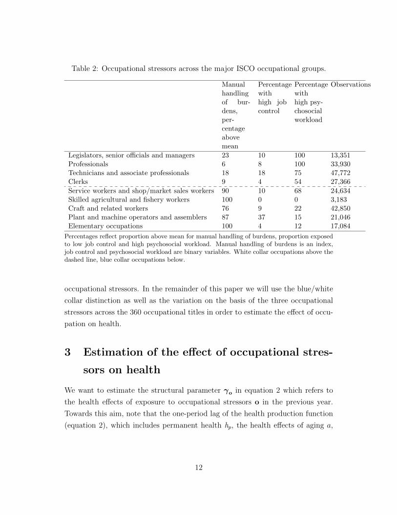
Table 2: Occupational stressors across the major ISCO occupational groups.
Manualhandlingof bur-dens,per-centageabovemean
Percentagewithhigh jobcontrol
Percentagewithhigh psy-chosocialworkload
Observations
Legislators, senior officials and managers 23 10 100 13,351Professionals 6 8 100 33,930Technicians and associate professionals 18 18 75 47,772Clerks 9 4 54 27,366
Service workers and shop/market sales workers 90 10 68 24,634Skilled agricultural and fishery workers 100 0 0 3,183Craft and related workers 76 9 22 42,850Plant and machine operators and assemblers 87 37 15 21,046Elementary occupations 100 4 12 17,084
Percentages reflect proportion above mean for manual handling of burdens, proportion exposedto low job control and high psychosocial workload. Manual handling of burdens is an index,job control and psychosocial workload are binary variables. White collar occupations above thedashed line, blue collar occupations below.
occupational stressors. In the remainder of this paper we will use the blue/white
collar distinction as well as the variation on the basis of the three occupational
stressors across the 360 occupational titles in order to estimate the effect of occu-
pation on health.
3 Estimation of the effect of occupational stres-
sors on health
We want to estimate the structural parameter γo in equation 2 which refers to
the health effects of exposure to occupational stressors o in the previous year.
Towards this aim, note that the one-period lag of the health production function
(equation 2), which includes permanent health hp, the health effects of aging a,
12

health investment m and shocks η, is:
ht+j−1 = hp +∑t+j−1
k=2
(ak + φt+j−1−k(γ ′ook−1 + γmm
θk−1 + ηk)
)(7)
Substituting equation 7 into equation 2 we obtain:
ht+j = (1− φ)(hp +
∑t+j−1
k=1(ak)
)+ at+j + γ ′oot+j−1 + γmm
θt+j−1 + φht+j−1 + ηt+j
(8)
Switching to individual notation and demeaning the covariates to eliminate the
time-invariant factors, we obtain a fixed effects within estimator:
hi,t+j − hi =φ(hi,t+j−1 − hi) + γ ′o(oi,t+j−1 − oi) + δ′(xi,t+j − xi) + εi,t+j (9)
where any unobserved heterogeneity that is constant over time and may be corre-
lated with occupation (such as permanent health hp in equation 2) is eliminated:
(1− φ)hp− (1− φ)hp = 0. Coefficient φ of the demeaned one period lag of health
can be interpreted as the decay parameter through which occupational choice o,
health investment m, and unforeseen shocks η in period t-2 and earlier periods
affect current health.
x is a vector of control variables consisting of age, age squared, age to the third
power, and wave dummies in order to control for common time trends. We assume
that the effect of age is smooth and can be approximated by an age polynomial
of the third degree. A less flexible approximation of the age effect, such as only
controlling for a linear term, would bias our estimates of γo if health deteriorates
more rapidly at older ages, and workers at older ages would be more or less likely
to be exposed to certain occupational stressors.
The error term is εi,t+j = γm(mθi,t+j−1 − mθ
i ) + ηi,t+j − ηi, which implies two
things. First, the ordinary least squares estimator of φ is biased since hi,t+j−1 is
correlated with ηi, and hi is correlated with ηi,t+j. Yet, importantly the estimator
is consistent for large T (Nickell, 1981; Bond, 2002). Second, the estimator of γo
is biased if occupation and health investment are correlated. The theory suggests
individuals simultaneously choose occupation and health investment, such that the
estimates should be interpreted as the sum of the structural effect of occupation
13
and health investment decisions related to occupation.
Self-reported health, on a five-point ordinal scale from poor to excellent, has
been shown to be a reliable predictor of mortality and morbidity (e.g. Idler and
Benyamini, 1997; Mackenbach et al. 2002). We use satisfaction with health
(on a 0-10 integer scale) as a proxy for health, which exhibits more variation
than the five-point measure. Ferrer-i-Carbonell and Frijters (2004) show that for
the variable that measures satisfaction with life on a ten point scale, assuming
ordinality or cardinality makes little difference, such that a linear specification is
acceptable. Reporting heterogeneity due to the fact that different subgroups may
report the same objective health status differently (Lindeboom and Van Doorslaer
2004), is eliminated by the individual fixed effect to the extent that it is time-
invariant.
Our estimates are based on variation in occupational stressors and health over
time within individuals for whom we observe occupation in the previous year
and health in the current year. Nonworking individuals generally remain in the
sample, except in the case of attrition due to mortality or nonresponse. Health-
related attrition leads to a downward bias – in absolute value – of our estimators
if individuals with the largest occupation-related health deterioration are more
likely to attrite. Our estimates should therefore be interpreted as a lower bound
on the true effect of occupational stressors.
4 Results
4.1 Main results
Table 3 shows the main results compared for five different models, where we first
present results for a dichotomous indicator for blue/white collar (columns 1 and 2)
and then present results where we break down occupation into three occupational
stressors (columns 3 to 5). To get an idea about the order of magnitude of the
coefficients, note that the average health deterioration of getting one year older
(obtained from an individual fixed effects regression of satisfaction with health on
age) is -.0666 (.0006) in our sample.
The bivariate association in column 1 between satisfaction with health and blue
14

or white collar occupation in the previous year tells us that blue collar workers are
in worse health, and that the size this health gap is similar to the average effect
of aging 25 months, which is a sizable and economically meaningful difference.
Column 2 shows the results for the model described by equation 9. Much of
the association appears to be driven by selection effects, as the estimate of the
causal effect is now -.0343 (.0171) compared to -.1418 (.0091) in column 1. We
conclude that the health effect of exposure to a blue collar instead of a white
collar occupation in the previous year is comparable to the average health effect
of aging six months. Column 3 breaks down occupation into three dimensions
of occupational stressors: manual handling of heavy burdens, job control, and
psychosocial workload in the preceding year. Manual handling of burdens and
low job control are associated with worse health, while workload is positively
associated with health. Given our theoretical model, we expect strong health-
related selection into occupation that could drive these associations. Column 4
shows estimates of the effects of these three occupational stressors according to the
specification in equation 9. We conclude that approximately fifty percent of the
negative association between manual handling of heavy burdens and health can
be explained by selection, and our point estimate (-.0275) of the causal effect of
a one standard deviation increase in manually handling heavy burdens compares
to a health effect of aging five months.
The estimates of the causal effects of psychosocial stressors (control possibili-
ties at work and workload) in column 4 are not significantly different from zero.
As we have seen in table 2 psychosocial workload was higher among white collar
workers and lower among blue collar workers with the exception of service work-
ers and shop and market sales workers. Socioeconomic factors, such as education,
influence both occupational rank – and therefore workload – and health status,
which leads to selection bias of the naıve estimator in column 3. A comparison
of the point estimates for workload in columns 3 and 4 confirms that selection
effects are important for psychosocial workload: the 95 percent confidence inter-
val of the causal estimate [-.0218, .0332] lies well below the confidence interval of
the association [.4593, .8430], plausibly because of the elimination of much of the
omitted variable bias that plagues the results in column 3.
We add a vector of occupational stressors interacted with age to the set of inde-
15

Table 3: Results.
Associa-tions forblue andwhitecollar
FE &LDV forblue andwhitecollar
Associa-tions forstressors
FE &LDV forstressors
FE &LDV forage inter-actions
(1) (2) (3) (4) (5)
Blue collar occupationat t-1
-.1418** -.0343*
(.0092) (.0171)
Manual handling of bur-dens at t-1
-.0567**(.0050)
-.0275**(.0090)
.0436(.0260)
Control possibilities att-1
.0582** -.0120 .1513*
(.0148) (.0217) (.0687)Workload at t-1 .0651** .0057 -.0358
(.0098) (.0140) (.0451)
Age * manual handlingof burdens at t-1
-.0019**(.0006)
Age * control possibili-ties at t-1
-.0042*(.0017)
Age * workload at t-1 .0011(.0011)
Health at t-1 .0985** .0985** .0983**(.0032) (.0032) (.0032)
Individual fixed effectsestimator controllingfor a third order agepolynomial and wavedummies
No Yes No Yes Yes
Observations 202,109 201,750 200,435 200,080 200,080R2 .0012 .5645 .0012 .5646 .5647
Main results for satisfaction with health. Panel-robust standard errors in parentheses. * indi-cates significance at 5 percent level, and ** at 1 percent level. Fixed effects specifications arecomputed by subtracting individual averages for each regressor. Reference category for columns1 and 2 is working in a white collar occupation. Intercept not shown.
16

pendent variables in column 5 of table 3 in order to investigate whether the causal
effect of occupational stressors differs by age. The model nests age-dependent and
age-independent effects: the coefficients of the interaction terms would be equal
to zero if the effects of the occupational stressors do not vary with age. The coef-
ficients of the noninteracted occupational stressors in rows three to five of column
5 cannot be interpreted directly, as they refer to the hypothetical effects of occu-
pational stressors at the age of zero. The coefficients of the interaction terms in
rows six to eight indicate how the effects of the occupational stressors change as
workers grow older.
Strikingly, predicted health deterioration due to a one standard deviation in-
crease in handling heavy burdens is equal to zero at the age of 23, but at the age
of 63, the point estimate of the effect is comparable to aging almost 14 months
(.0436-.0019*63=-.077). Low job control has a negative effect after the age of
36: being in a job with low instead of high job control at the age of 63 leads
to a predicted health deterioration comparable to the effect of aging 20 months
(.1513-.0042*63=-.1133). We conclude that the effect of manual work and job
control is age-dependent. The effect of the interaction of workload and age is not
significantly different from zero, possibly due to our crude, dichotomous measure
of workload or because workload is only important for a subset of occupations.
The health effects of past exposure to occupational stressors cannot simply
be added to obtain cumulative effects. Under quite demanding assumptions, we
can compute cumulative health effects by using the estimated coefficient of the
lagged dependent variable, φ in equation 2, which by assumption is the uniform
exponential decay rate at which past health investment, occupational stressors,
and shocks affect current health. The point estimates of φ in table 3 suggest
that roughly ten percent of the occupation-related health damage in period t-2
persists in period t. Using the point estimates in column 5, the point estimate of
health damage at the age of 65 due to a one standard deviation increase in manual
handling of heavy burdens between ages 60 to 64 is∑64
k=60 .098364−k(.0436−.0019∗k) = −.0865, which is comparable to the average health effect of aging almost
16 months. Likewise, the point estimate of the effect of working in low control
occupations between ages 60 to 64 is -.1398, which is comparable to the effect of
aging 23 months.
17
4.2 Robustness checks
Individuals in different occupations may have different biological aging rates, while
we have assumed uniform aging effects in the preceding analyses. If the health of
individuals in manual occupations would decline more strongly, our results would
overestimate the harmful effects of physical stressors. In column 1 of table 4 we
allow for different aging rates by interacting an education dummy with a third
degree age polynomical. Our estimates are similar to our findings in table 3, and
we find no significant differences in the biological aging rate between individuals
with high and low educational attainment. The estimator of the coefficient of the
lagged dependent variable is consistent if the number of time periods in the sample
goes to infinity. Our sample spans 26 years and is unbalanced: it includes individ-
uals who are observed in a lower number of waves. We repeat our analysis for a
subsample of 10,373 individuals who are employed in at least nine years in order
to counter the downward bias of the estimator of the lagged dependent variable
that plagues short panels (Bond, 2002). The number of person-wave observations
drops from 200,080 in our baseline specification in column 5 of table 3 to 136,470
in column 2 of table 4. The coefficients of the (age interacted) occupational stres-
sors are similar to those in our baseline specification. However, the coefficient of
lagged health is now larger than before, suggesting that past health investment,
occupational stress, and health shocks are more persistent than appeared in our
analysis of the full sample. We conclude that our estimates of the effects of occu-
pational stressors are robust across specifications, but that an analysis on the full
sample leads to underestimation of the coefficient of lagged health. We may have
underestimated the cumulative effects of occupational history by underestimating
φ, and the predictions in the previous paragraph provide – in absolute terms –
the lower bounds on the effects, which means that the true health effects may be
even larger.
Angrist and Pischke (2009) voice worries about the violation of strict exogene-
ity in fixed effects dynamic models, particularly when using short panels. They
propose to check robustness by separately estimating both a fixed effects and a
lagged dependent variable model. Column 3 of table 4 presents results from a
fixed effects model without a lagged dependent variable. With respect to equa-
tion 9, the error term would now include the deviations of the effects of health
18

Table 4: Robustness.
Controlforeducation-specificagingtrends
Onlyindi-vidualswithT ≥ 10
FE LDV
(1) (2) (3) (4)
Manual handling of burdensat t-1
.0317(.0268)
.0447(.0276)
.0534*(.0262)
.0435**(.0149)
Control possibilities at t-1 -.1350 .1911** -.1562* -.0707(.0696) (.0728) (.0691) (.0447)
Workload at t-1 -.0370 -.0445 -.0404 -.0645*(.0463) (.0480) (.0455) (.0288)
Age * manual handling of bur-dens at t-1
-.0016**(.0007)
-.0019**(.0007)
-.0022**(.0007)
-.0023**(.0004)
Age * control possibilities att-1
.0039*(.0017)
.0049**(.0018)
.0044*(.0017)
.0008(.0011)
Age * workload at t-1 .0011(.0011)
.0014(.0012)
.0012(.0011)
.0029**(.0007)
Health at t-1 .0976** .1378** .5420**(.0032) (.0034) (.0023)
Third order age polynomialand wave dummies
Yes Yes Yes Yes
Third order age polynomialinteracted with age
Yes No No No
Individual fixed effects Yes Yes Yes NoEducation and gender No No No YesObservations 196,935 152,244 200,435 196,935R2 .5647 .5647 .5604 .3351
Robustness checks for satisfaction with health. Panel-robust standard errors in parentheses. *indicates significance at 5 percent level, and ** at 1 percent level. Fixed effects specificationsare computed by subtracting individual averages for each regressor. Second column on sampleof individuals who are observed in at least 10 waves. Intercept not shown.
19

investment, occupational stressors, and health shocks before period t-1 from their
individual averages. If a past health shock would have a negative effect on cur-
rent health and lead to higher occupational stress in the previous period, we would
overestimate the effect of occupational stressors since this leads to additional cor-
relation between o and the error term. The point estimates in column 3 suggest a
somewhat stronger effect of manual handling of burdens and job control at older
ages than the baseline specification, but these may result from the bias caused by
past events that affected health. The lower R2 compared to the baseline specifi-
cation in column 5 of table 3 indicates that this model explains less variation in
the outcome variable, possibly because the health effects of omitted variables are
no longer proxied by lagged health.
In a model in which we control for a lagged dependent variable, but not for
individual-specific fixed effects, the estimator of the decay parameter φ in equation
9 is biased towards one: all past deviations from the steady state of health “die
out” while the time-invariant individual fixed effects are constant over time. In
this specification we therefore overestimate the impact of past events on current
health, and we only partly control for unobserved time-invariant heterogeneity.
By not subtracting averages in equation 9, the error term now includes (1−φ)hp,
which may be correlated with lagged health and the occupational characteristics.
In order to proxy for time-invariant unobserved factors otherwise picked up by the
fixed effect, we control for years of schooling and gender. Our estimates are now
mostly driven by variation between individuals a moment in time. The relatively
low R2 in column 4 of table 4 reflects how this only partially enables us to control
for unobserved heterogeneity. The coefficient of the interaction between age and
manual handling of burdens is similar to our earlier results, but the coefficient
of the interaction between age and job control is no longer significant. Workload
now seems to have a positive effect, but this may be due to the fact that, by
not controlling for individual-specific fixed effects, we insufficiently control for the
selection of healthy individuals into occupations characterized by high workload.
Other methods have been proposed to consistently estimate γo in equation 9 in
short panels, of which the so-called Arellano-Bond estimator (Arellano and Bover,
1995; Blundell and Bond, 1998) is the most prominent one. The Arellano-Bond
estimator is based on the first-difference estimator. Most important assumption
20

is that the second and further lags of health, are uncorrelated with the first differ-
ences of the error term and can be used as instrumental variables for ht−1 − ht−2.
Unfortunately, in our case the Arellano-Bond test for autocorrelation rejects this
assumption, which is perhaps not so surprising since in the case of health, using
lagged values as instruments seems hard to justify. Chronic illnesses or the in-
troduction of a new medical drug may progressively affect health over time. This
leads to second or higher order serial correlation in the differenced error term and
violation of the exogeneity assumption. In an attempt to overcome this problem
one could include more lags of the regressors in the model and use further lags
of the instruments in order to attempt to get rid of the autocorrelation in the er-
ror term, but we still find higher order autocorrelation in these models, rejecting
validity of the instruments.7
5 Conclusion
We find that exposure to both high physical occupational stress and low job
control has a negative effect on health. The immediate effect of exposure to a
one standard deviation increase in the degree of handling heavy burdens (e.g.
from mail sorter to a bricklayer) during one year is comparable to aging five
months. This effect becomes stronger with age: just before reaching the retire-
ment age, a similar increase in handling heavy burdens is comparable to aging
fourteen months. Low job control is equally harmful to health, but only after age
36. After age 60, the immediate effect of low job control (e.g. nurse instead of
physiotherapist) is equivalent to aging 20 months. The estimated causal effect of
7Limiting the number of waves could give us the false illusion that serial correlation of theerror term is not a problem, simply because of the low power of the test. Blundell and Bondand Michaud and Van Soest (2008) used short panels of six waves, and they “use up” even morewaves because of the inclusion of lagged values of the dependent variable. The autocorrelationtests in these studies do not reject the assumption of no autocorrelation in the error term butthis could be due to limited test power with the small number of waves. If we include one andtwo period lags of the dependent variable (Michaud and Van Soest (2008),we find no secondorder autocorrelation, but we do find autocorrelation of the third order which would still violatethe Arellano Bond assumptions. Including third or fourth lags seems to shift downwards theorder of autocorrelation, instead of solving the problem. Performing the Sargan test may notbe very informative since this test assumes that at least one instrument is exogenous, which isan assumption we are not willing to make.
21

carrying heavy burdens accounts for roughly 50 percent of the bivariate associa-
tion between occupation and health. This implies that selection into occupation
by prior health and/or other factors such as education accounts for the other half
of the observed association.
We derive the empirical specification from a theoretical model of occupation
and health over the life cycle and outline the conditions under which we can obtain
causal estimates using a detailed longitudinal dataset over many time periods (26
years). We show how a fixed effects lagged dependent variable model neutralizes
several time-invariant and time-varying sources of selection bias and argue that
the resulting estimators are preferable in the absence of exogenous variation in
occupational stressors. Moreover, our study generalizes across the labor force,
in contrast to local effect estimates based on a particular reform that affected
only part of the employed population. We show that the coefficient of the lagged
dependent variable should be interpreted as a decay parameter that captures the
effects of past unobserved factors – which affected health in the previous period
but could also have affected occupational choice – on current health.
We were able to separate the health effects of physical and psychosocial stres-
sors by linking German longitudinal data on occupational titles to Finnish data
on occupational stressors on the level of detailed occupational titles. However,
as we did not observe individual levels of health investment, we were unable to
disentangle the effects of the occupational stressors and any health investment
that was made in response to occupational choice. Our estimates should therefore
be interpreted as the sum of the direct effect of occupation and the health effect
of any behavioral response to occupational choice.
Occupational health and safety policies, career development programs, and
retirement policies should be based on the insight that exposure to physically
demanding manual handling of burdens and low job-control is harmful to health
at older ages. Shielding older workers from these conditions prevents health de-
terioration among vulnerable groups of workers and is likely to have a protective
effect against illness-related absenteeism and labor force exit due to disability.
22

References
Altonji, J. G., Elder, T. E., and Taber, C. R. (2005). Selection on observed and
unobserved variables: Assessing the effectiveness of catholic schools. Journal of
political economy, 113(1):151–184.
Angrist, J. D. and Pischke, J.-S. (2009). Mostly Harmless Econometrics: An
Empiricist’s Companion. Princeton University Press.
Arellano, M. and Bover, O. (1995). Another look at the instrumental variable
estimation of error-components models. Journal of Econometrics, 68(1):29 –
51.
Blundell, R. and Bond, S. (1998). Initial conditions and moment restrictions in
dynamic panel data models. Journal of Econometrics, 87(1):115 – 143.
Bond, S. R. (2002). Dynamic panel data models: a guide to micro data methods
and practice. Portuguese Economic Journal, 1(2):141–162.
Bongers, P. M., Hulshof, C. T. J., Dijkstra, L., Boshuizen, H. C., Groenhout, H.
J. M., and Valken, E. (1990). Back pain and exposure to whole body vibration
in helicopter pilots. Ergonomics, 33(8):1007–1026. PMID: 2147003.
Case, A. and Deaton, A. S. (2005). Broken down by work and sex: How our
health declines. In Analyses in the Economics of Aging, NBER Chapters, pages
185–212. National Bureau of Economic Research, Inc.
Choo, E. and Denny, M. (2006). Wearing out – the decline in health. Working
Papers tecipa-258, University of Toronto, Department of Economics.
Cutler, D. M., Lleras-Muney, A., and Vogl, T. (2008). Socioeconomic status and
health: Dimensions and mechanisms. Number 14333 in Working Paper Series.
Fletcher, J. M. and Sindelar, J. L. (2009). Estimating causal effects of early
occupational choice on later health: Evidence using the psid. Working Paper
15256, National Bureau of Economic Research.
Fletcher, J. M., Sindelar, J. L., and Yamaguchi, S. (2011). Cumulative effects of
job characteristics on health. Health Economics, 20(5):553–570.
23
Galama, T. and van Kippersluis, H. (2010). A theory of socioeconomic disparities
in health over the life cycle.
Goodman, E. (1999). The role of socioeconomic status gradients in explain-
ing differences in us adolescents’ health. American Journal of Public Health,
89(10):1522–1528.
Grossman, M. (1972). On the concept of health capital and the demand for health.
Journal of Political Economy, 80(2):223–255.
Kauppinen, T., Toikkanen, J., and Pukkala, E. (1998). From cross-tabulations
to multipurpose exposure information systems: a new job-exposure matrix.
American journal of industrial medicine, 33(4):409–417.
Kelly, I. R., Dave, D. M., Sindelar, J. L., and Gallo, W. T. (2011). The impact
of early occupational choice on health behaviors. Review of Economics of the
Household, pages 1–34.
Kunst, A. E., Groenhof, F., Andersen, O., Borgan, J. K., Costa, G., Desplanques,
G., Filakti, H., Giraldes, M. d. R., Faggiano, F., Harding, S., et al. (1999).
Occupational class and ischemic heart disease mortality in the united states
and 11 european countries. American Journal of Public Health, 89(1):47–53.
Kunst, A. E., Groenhof, F., and Mackenbach, J. P. (1998). Mortality by occupa-
tional class among men 30–64years in 11 european countries. Social science &
medicine, 46(11):1459–1476.
Lewbel, A. (2012). Using heteroscedasticity to identify and estimate mismeasured
and endogenous regressor models. Journal of Business & Economic Statistics,
30(1).
Mackenbach, J. P., Bos, V., Andersen, O., Cardano, M., Costa, G., Harding,
S., Reid, A., Hemstrom, O., Valkonen, T., and Kunst, A. E. (2003). Widen-
ing socioeconomic inequalities in mortality in six western european countries.
International journal of epidemiology, 32(5):830–837.
24

Mackenbach, J. P., Kunst, A. E., Cavelaars, A. E., Groenhof, F., and Geurts,
J. J. (1997). Socioeconomic inequalities in morbidity and mortality in western
europe. The Lancet, 349(9066):1655–1659.
Marmot, M. G., Stansfeld, S., Patel, C., North, F., Head, J., White, I., Brunner,
E., Feeney, A., Marmot, M. G., and Smith, G. D. (1991). Health inequalities
among british civil servants: the whitehall ii study. The Lancet, 337(8754):1387
– 1393.
Michaud, P.-C. and Van Soest, A. (2008). Health and wealth of elderly couples:
Causality tests using dynamic panel data models. Journal of Health Economics,
27(5):1312–1325.
Morefield, B., Ribar, D. C., and Ruhm, C. J. (2012). Occupational status and
health transitions. The BE Journal of Economic Analysis & Policy, 11(3).
Nickell, S. (1981). Biases in dynamic models with fixed effects. Econometrica:
Journal of the Econometric Society, pages 1417–1426.
Ravesteijn, B., van Kippersluis, H., and van Doorslaer, E. (2013). Long and
healthy careers? the relationship between occupation and health.
Smith, R. (1974). The feasibility of an” injury tax” approach to occupational
safety. Law and Contemporary Problems, 38(4):730–744.
Viscusi, W. (1978). Labor market valuations of life and limb: Empirical evidence
and policy implications. Public Policy, 26(3):359–386.
25


