May 1992 Report No. STAN-CS-92-1444
AD-A268 387 Also numbered CSL-TR-92-542
(OV Thesis
Multiprocessor Performance Debuggingand Memory Bottlenecks
by
Aaron J. Goldberg
DTICSEL E C T E
AUG24 1993 Dv EDepartment of Computer Science . -....
Stanford University
Stanford, California 94305
93-19530ImlllIllIE93 8 23 023

REPORT DOCUMENTATION PAGE 0148 ft. 070W4189OW.C too" V~fl9 iW4 OWiftv"~m mof u~ 00 *l mis 90Wl a I feftw Vw quggiw. iWahm Ve Wo off g o Wsa mw .etm AIM 20urdf
pmee~9 a. OW6 SM .61* s. &V demo" #~ON ::i:lb 4 W~fmati, ~SWA 'eaSlfmtw m..m~em e
avi""0^1!`3 ow. 07• 0 , V
,* ,, - r - - .. . . = ' m ',- UiO ".. .S. W • m S PIm q m s b 6 1ff 5~q . P m s mSl~' in P N U Ol I 5I• W qSin~ m. iDC MI i I.
1. AGENCY US" ONLY "so". RI E PORT DATE P. R~ORT TP ANO OATES COvEuE
4. TITLI AND SUBT1ITE S; FUNDING NUMBERSF 6N00039-91-C-0138
pL7W/DAY baTTLO#LC6K5
. AUTNOORS)
AAftoA' J. CO0o3Cn67. PERIFORMIIEG ORGANIZATION NAME(S) AND AODRESS([S) B. PERFORMING ORGANIZATION
Stanford University REPORT NUMBERComputer Systems LaboratoryCenter for Integrated Systems STAN-CS-92-1444
Stanford, CA 94305-4070 CSL-TR-92-542
g. SPONSORING/ MONITORING AGENCY NAMI(S) AND ADORESS(IS) 10. SPONSORING/MONITORING, 2ARPA/Llq 11 AGENCY RUPO"T NUMBER
3FairfaxArlný4", VA 22203-1714
I1. SUPPLIMENTARY NOTMS
I1a. DISTRIBUTION i AVAILABILITY STATEMUNT 1211. DISTRIBUTION CODE
i. ABSTRACT (Maxmum 200 woms)Driven by the computational demands of scientists and engineers, computer architects are building in-
creasingly complex multiprocessor systems. However, while the peak Gigaflop ratings of such systems is oftenimpressive, the actual performance of initial implementations of applications can be disappointing. To makethe task of performance debugging manageable, tools are needed that can analyse program behavior andreport sources of performance loss. This thesis offers techniques for building such tools for shared memorymultiprocessors. Previous efforts to build performance debugging systems for shared memory multiproces-sors had two shortcomings. First, though memory hierarchy performance is often critical to whole programperformance, most tools cannot distinguish time the CPU is computing from time when it is stalled wait-ing on the memory hierarchy. Second, other tools often significantly perturb a program's execution. Thisdissertation addresses both of these problems. I describe software instrumentation that typically increasesprogram execution time by less than 10%, while collecting a detailed profile of where processors are doingwork, waiting for work, or stalled waiting on the memory hierarchy. A window-based user interface allows theuser to interpret the profile, viewing compute, memory, and synchronization bottlenecks at increasing levelsof detail, from a whole program level down to the level of individual procedures, loops, and synchronizationobjects. Several multiprocessor case studies are included to to illustrate the features of the tool.
14. SURIJIT TER.MS IS. NUMBER Of PAGES
16. PRICE CODE
17. SICURITY CLASSIFICATION 1l. SICURITY CLASSIFICATION It l CURIrY CLASSIFICATION 10. LIMITATION OF ABSTRACTOf RIPORT OF THIS PAGE OF ABSTRACT
INSk 7S4•0I.Qi0.agoSg Sranas';ot¶ ;91 Vlo 2.69)

MULTIPROCESSOR PERFORMANCE DEBUGGING
AND MEMORY BOTTLENECKS
A DISSERTATION
SUBMITTED TO THE DEPARTMENT OF COMPUTER SCIENCE
AND THE COMMITTEE ON GRADUATE STUDIES
OF STANFORD UNIVERSITY
IN PARTIAL FULFILLMENT OF THE REQUIREMENTS
FOR THE DEGREE OF
DOCTOR OF PHILOSOPHYAcCecioa For
NTIS CRA&IDiIC TABU a mouncedJ istfifca-tion . .. .........................
By .............
Di-t ibition IBy Availability Codes
Aaron J. Goldberg Avi ado
May 1992 Dist Special
urIc QU&LtYr s 8!

© Copyright 1992
by
Aaron J. Goldberg
ii

I certif, that I have read this thesis and that in my opinion
it is fully adequate. in scope and in quality., as a dissertation
for the degre Doctor of Philos hy.
I certify that I have read this thesis and that in my opiLion
it is fully adequate. in scope and in quality, as a dissertation
for the degree of Doctor of Philosophy.
ýKopGuota
I certify that I have read this thesis and that in m% opinion
it is fully adequate. in scope and in quality, as a dissertation
for the degree of Doctor of Philosophy.
1dseph Oliger .,
Approved for the University Committee
on Graduate Studies:
iii.
i5
Abstract
Driven by the computational demands of scientists and engineers, computer architects
are building increasingly complex multiprocessor systems. However, while the peak
Gigaflop rating of such systems is often impressive, the actual performance of initial
implementations of applications can be disappointing. To make the task of performance
debugging manageable, tools are needed that can analyze program behavior and report
sources of performance loss. This dissertation describes techniques for building such
tools for shared memory multiprocessors.
Pievious efforts to build performance debugging systems for shared memory multi-
processors had two shortcomings. First, though memory hierarchy performance is often
critical to program performance, most tools cannot distinguish the time the CPU is com-
puting from the time when it is stalled waiting on the memory hierarchy. Second, many
tools significantly perturb a program's execution adding 50% or more overhead, making
it difficult to measure the behavior of the original uninstrumented code. This dissertation
addresses both of these problems. Our software instrumentation system, Mtool, typically
increases program execution time by less than 10% while collecting a detailed profile of
where processors are doing work, waiting for work, or stalled waiting on the memory
hierarchy. The overhead of the instrumentation is kept to less than 10% (on average) by
exploiting a basic block count profile to guide Mtool in selecting the best instrumentation
points for each program. A window-based user interface allows the user to interpret the
profile, viewing compute, memory, and synchronization bottlenecks at increasing levels
of detail, from a whole program level down to the level of individual procedures, loops,
and synchronization objects.
Current multiprocessors often have features like per-processor multi-level caches,
iv

buffers, complex interconnection networks, and banked memories that dynamically inter-
act to determine memory system performance. Mtool uses a memory overhead detection
technique that is independent of this complexity. By comparing an ideal CPU time profile
based on basic block count information against an actual execution time profile, Mtool
can isolate memory system effects in just over the time to execute the original code
twice. This technique represents a significant improvement over previous simulation-
based methods that take 10-1000 times longer to run than the the programmer's actual
code.
Mtool is in active use by several groups of parallel programmers at Stanford. We sum-
marize their experiences with the tool, exploring which attention focusing mechanisms
are most important, describing actual techniques by which memory and synchroniza-
tion behavior were improved, and providing real data on the importance of memory and
synchronization overheads in several multiprocessor applications.
V

Acknowledgements
I would like to thank those people whose support, assistance, and encouragement made the
writing of this thesis an enjoyable task. In particular, I would like to thank my principal
adviser, John Hennessy, for his broad guidance and constructive comments. I would also
like to thank Anoop Gupta and Joe Oliger for serving on my reading committee. And
thanks to David Wall and DECWRL for supporting the initial implementation of this
thesis work and to the DASH group at Stanford for advice and feedback. Ed Rothberg
provided valuable discussions and acted as Mtool's first user and the two major case
studies of Chapter 5 were contributed by Penny Koujianou and Andrew Erlichson.
Finally, I would like to express my gratitude to the friends at Stanford who made
the experience happy and worthwhile. First and foremost I thank Penny for giving me
constant support and an incentive to finish. Also, my sincere thanks to the friends,
housemates, officemates, and regular lunch bunch participants (Ken, Gidi, and Adnan)
whose camaraderie made my stay at Stanford more pleasant.
I would also like to acknowledge support from an NSF graduate fellowship and
DARPA grant N00014-87-K-0828.
vi

Contents
Abstract iv
Acknowledgements vi
1 Introduction 1
1.1 Shared Memory Multiprocessing ...... ..................... 1
1.2 Performance Debugging Tools ............................. 4
1.2.1 Static Analysis .................................. 6
1.2.2 Simulation ........ ............................. 7
1.2.3 Hardware and Software Instrumentation ................... 7
1.3 Scope and Contributions ................................ 11
2 Detecting Memory Overhead in Sequential Code 14
2.1 Ideal Compute Tume Profiles ............................ 15
2.2 Isolating Memory Overheads with Mprof ...................... 16
2.3 Better Clock Resolution ....... .......................... 23
2.4 Effectiveness of High Resolution Clocks ...................... 29
3 Reduced Cost Basic Block Counting 32
3.1 Controlling Counter Overhead ............................. 33
3.1.1 Minimum Overhead Labelling Algorithm ................. 35
3.1.2 Counter Costs ................................. 38
3.1.3 Empirical Results .............................. 41
3.1.4 Heuristics ................................... 46
vii

3.2 Compensating for Instrumentation Overheads ................... 53
3.3 Conclusions on Lightweight Profiling ........................ 56
3.4 Counter Perturbation in Parallel Programs ..................... 57
4 Mtool: A Multiprocessor Performance Debugger 62
4.1 Compute Time and Memory Overhead ........................ 63
4.2 Synchronization Overhead ................................ 65
4.2.1 ANL Macros ................................... 67
4.2.2 Compiler Parallelized Fortran ........................ 70
4.3 Parallel Overhead ........ ............................. 71
4.4 Attention Focusing Mechanisms ............................ 72
4.4.1 User Interface ....... ........................... 72
4.4.2 Comparison with Other Tools ........................ 75
5 Case Studies 80
5.1 Fortran Case Study ........ ............................ 80
5.2 Porting PSIM4 to DASH ....... ......................... 89
5.3 Write Buffer Effects ....... ............................ 95
5.4 Side by Side Comparison ....... ......................... 96
6 Conclusions 100
6.1 Mtool Limitations ....... ............................. 101
6.2 Further Research . . . . .. ... .................. 103
6.2.1 Attention Focusing and Feedback-Based Code Transformation . . 103
6.2.2 Selective Tracing ...... ......................... 104
6.2.3 Exploiting Hardware Instrumentation ................... 104
A Mprof Results for the SPECmarks 106
A.1 Discussion of Memory Overheads .......................... 116
Bibliography 118
viii
List of Tables
1 MP3D Aggregate Execution Times in Seconds .............. 3
2 Software Instrumentation Based Tools ........................ 93 Summary of Performance Debugging Approaches ..... ............ 11
4 CPU Utilizations of the SPECmarks .......................... 19
5 Reducing Memory Overhead in vpenta ...................... 22
6 Lines of Source Code vs. Percentage of Total Memory Overhead . . .. 24
7 Counter Cost Per Execution in CPU Cycles ..................... 40
8 Counter Increments and Minimum Instrumentation Overheads ...... .. 429 Register Scavenging Percentage Overheads ..................... 54
10 Effect of Instrumentation on Memory System ................... 55
11 Possible Effects of Instrumentation ...... .................... 58
12 Instrumentation Overheads for Parallel Programs ................. 61
13 Tuning ANL Macro Synchronization ..... ................... 7014 Outline of CARS Case Study ...... ....................... 89
15 Summary of PSIM4 Case Study ...... ..................... 9416 cahift Performance ....... ........................... 96
ix
List of Figures
1 A Typical Shared Memory Multiprocessor ................ 2
2 Creating a Memory Overhead Profile with Mprof ................. 16
3 Mprof output for eqntott ....... ........................ 18
4 A Critical Loop inv•penta ............................... 20
5 Using Explicit Clock Reads with Mprof ....................... 26
6 Improvement in Memory Operation Coverage ................... 30
7 A Program and Its Control Flow Graph ........................ 35
8 Modifying a Directed Graph So It Has an Undirected Analog ...... .. 37
9 Transformation to Add Node Counter Edges ................... 41
10 Finding the "Average" Cost of Instrumenting Independent Edges .... 46
11 A Graph That Defies Heuristics ............................ 47
12 Applying the Heuristic to a Loop-Free Graph ................... 48
13 The Cost of Measuring A Loop ............................ 49
14 Creating a Memory Overhead Profile with Mtool. ................ 65
15 Sources of Synchronization Loss ...... ..................... 66
16 Mtool Summary Window ....... ......................... 74
17 Mtool Procedure Histogram ....... ........................ 74
18 Mtool Text and Info Windows ............................. 75
19 Summary Window for CARSO ....... ...................... 81
20 Procedure Histogram for CARSO ...... ..................... 82
21 Source Code Window for CARSO ........................... 83
22 Summary Window for CARS1 ....... ...................... 84
23 Summary Window and Procedure Histogram for PCARSO ........ .. 85
X
24 Summary Window for PCARS1 ..................... 86
25 Procedure Histogram for PCARSI ....... .................... 87
26 Source Code Window for PCARS1 ...... .................... 87
27 Creating a Balanced Static Schedule ...... ................... 88
28 Summary Window for PCARS.BEST ........................ 89
29 Summary Window and Histogram for PSIM4.0 .................. 91
30 Call Graph Nodes for .doprnt and sprintf .................. 91
31 Summary Window and Histogram for PSIM4.1 .................. 93
32 Source Code Window for PSIM4.1 ........................... 94
33 Comparison of nvst Histogram for One and Four Processor Runs . . .. 97
?4 Comparison of Histogram for One and Eight Processor Runs ........ 98
xi
Chapter 1
Introduction
The complexity of multiprocessor systems has been increasing more quickly than the
sophistication of parallel programming environments. Because of this "software gap,"
many programmers find it difficult to understand why the achieved performance of their
parallel applications is often well below the peak performance of the actual hardware. To
make the task of performance debugging manageable, tools are needed that can analyze
program behavior and report sources of performance loss. This dissertation describes
techniques for building such tools for shared memory multiprocessors. The introduc-
tory chapter gives an overview of previous developments in multiprocessor performance
debugging and demonstrates why more work is needed. Our claim is that three prob-
lems must be addressed to make tools effective. First, a technique is needed that can
distinguish time spent computing from time spent waiting on the memory hierarchy or
in synchronization. Second, software instrumentation cannot substantially perturb the
programs that are being monitored; otherwise the recorded data may be meaningless.
Finally, instrumentation can generate almost unlimited data so there is a critical need for
interfaces that assist the user in navigating through the mass of data that is collected.
1.1 Shared Memory Multiprocessing
The focus of this work is on performance debugging applications written for shared
memory multiprocessors that provide a global address space. Figure 1 depicts a typical
• ma m |1

CHAPTER 1. INTRODUCTION 2
P1 P8
Lev-1 Cache 64 Kbytes Lev-1 Cache 64 Kbytes
Lev-2 Cache 256 Kbytes Lev-2 Cache 256 Kbytes
Figure 1: A Typical Shared Memory Multiprocessor
system. A number of processors communicate over a shared bus. Each processor has
a large multilevel cache to reduce traffic on the bus; the caches are kept consistent via
a bus snooping protocol. The figure actually represents the Silicon Graphics (SGI) 380
multiprocessor that will be used in many of the studies later in this dissertation.
The advantage of shared memory multiprocessors is that the global address space
model reduces the logical complexity of programming. At times, however, the sim-
ple model can be deceptive because while memory is logically shared, access time to
the memory is not uniform. Real machines have features like per-processor multi-level
caches, buffers, complex interconnection networks, and banked memories that dynami-
cally interact to determine memory system performance. In today's NUMA (non-uniform
memory access) systems, some memory references hit in local cache and are cheaper than
others; and global data references may involve costly accesses across a shared communi-
cation medium (bus or interconnection network). For example, the SGI system depicted
above has a 14 cycle first-level cache miss penalty while a second level miss stalls the
processor for at least 40 cycles. The Stanford DASH machine where we performed the
work for the case study of Section 5.2 has a penalty of 28 cycles for a second level cache
miss and over 100 cycles when the data must be fetched from a remote cluster. The
penalties increase when there is contention. It is also worth noting that the continuing
CHAPTER 1. INTRODUCTION 3
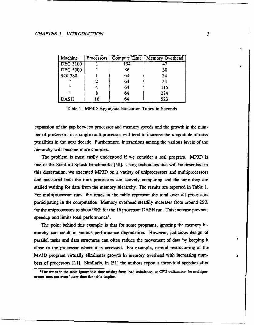
Machine Processors Compute Time Memory OverheadDEC 3100 1 134 47DEC 5000 1 86 30SGI 380 1 64 24
"2 64 54"4 64 115"8 64 274
DASH 16 64 523
Table 1: MP3D Aggregate Execution Times in Seconds
expansion of the gap between processor and memory speeds and the growth in the num-
ber of processors in a single multiprocessor will tend to increase the magnitude of miss
penalities in the next decade. Furthermore, interactions among the various levels of the
hierarchy will become more complex.
The problem is most easily understood if we consider a real program. MP3D is
one of the Stanford Splash benchmarks [58]. Using techniques that will be described in
this dissertation, we executed MP3D on a variety of uniprocessors and multiprocessors
and measured both the time processors are actively computing and the time they are
stalled waiting for data from the memory hierarchy. The results are reported in Table 1.
For multiprocessor runs, the times in the table represent the total over all processors
participating in the computation. Memory overhead steadily increases from around 25%
for the uniprocessors to about 90% for the 16 processor DASH run. This increase prevents
speedup and limits total performance'.
The point behind this example is that for some programs, ignoring the memory hi-
erarchy can result in serious performance degradation. However, judicious design of
parallel tasks and data structures can often reduce the movement of data by keeping it
close to the processor where it is accessed. For example, careful restructuring of the
MP3D program virtually eliminates growth in memory overhead with increasing num-
bers of processors [11]. Similarly, in [51] the authors report a three-fold speedup after
1The ames in the table ignore idle time arising from load imbalance, so CPU utilizations for multipro-ceuor rtus are even lower than the table implies.

CRAPER 1. INTRODUCTION 4
optimizing a sparse Cholesky factorization algorithm to reduce memory traffic and keep
data local to processors. In [17] the authors describe how simple blocking techniques
can significantly improve memory hierarchy performance.
Two other promising techniques for reducing memory overhead in shared memory
multiprocessors are software controlled prefetch and eliminating false sharing. With
prefetch, we can issue a non-blocking request for data to be brought nearer to the proces-
sor; when the data is actually needed, it can be accessed more quickly. Studics like [47]
have shown that software controlled prefetching of data can hide the latency of the mem-
ory hierarchy, improving the performance of some applications by a factor of two or
more. Finally, several studies have demonstrated that "false" sharing of cache lines is a
common source of poor memory system performance that can often be eliminated. False
sharing arises when cache lines contain multiple data items while cache coherence is
maintained on a per line basis. In the worst case, multiple processors are reading and
writing different data items in the same line. Since the coherence protocol works at the
line level, it will repeatedly copy the shared line between processors, even though the
processors are actually working on independent data items. False sharing can often be
eliminated by simple transformations like data replication or padding [15, 25, 621.
Of course, for programmers to apply these performance enhancing transformations,
they must know the location and severity of memory bottlenecks in their code. The task of
understanding memory overhead is particularly complex because sources of performance
loss interact. Often we find a tradeoff between data locality and parallelism: if a task's
working set had been loaded into the local cache of processor I which is already working
on another task while processor 2 is idle, is it better to schedule the task on 2 or will
the memory overhead of loading 2's cache dominate any performance improvement? To
understand this tradeoff, the programmer needs to have information on both memory and
synchronization overhead.
1.2 Performance Debugging Tools
The previous examples provide a glimpse into the complex process of tuning parallel
programs to increase performance. In this section we survey the literature on tools that

CHAPTER 1. JNTRODUCTION 5
assist the programmer in this process. We categorize these performance debugging tools
according to two fundamental attributes: what they measure and how they measure it.
There are literally dozens of tools which together measure hundreds of individual
performance characteristics from low level statistics like number of instruction buffer
fetches to aggregate metrics like total execution time. Despite the variety of attributes
measured, we have found that most tools eventually deliver their measurements in terms
of the following execution time taxonomy:
1. Compute Time: The processor is performing work.
2. Memory Overhead: The processor is stalled waiting for data or communication.
3. Synchronization Overhead: The processor is idle waiting for work.
4. Extra Parallel Work: The processor is performing work not present in the se-quential code.
The existence of this higher level taxonomy is not surprising because performance tools
are structured to deliver information in terms that are useful and intuitive to the program-
mer. Thus, the execution time taxonomy reflects a common underlying programming
model for shared memory multiprocessors.
Note, however, the categories in the taxonomy are defined rather broadly so some
judgement may be required to classify particular measurements. In the MP3D example
above we saw that memory overhead increased with the number of processors involved
in the computation. According to this taxonomy, this increase could be viewed as extra
parallel work rather than memory overhead. Moreover, we can speak both of extra parallel
work with respect to a sequential run of the parallel program and of extra work relative
to the best possible sequential implementation of the program. Chapter 4 elaborates
on the taxonomy and tries to resolve such ambiguities. Specifically, it suggests using
side-by-side profile comparisons to detect both kinds of extra work.
A second problem with the categories in the taxonomy is their bias toward CPU
bound computation. The taxonomy neglects time spent in operating systems services and
I/O; this dissertation concentrates on user level issues. Descriptions of tools directed at
systems level bottlenecks can be found in [26, 28, 33, 45, 52).
Despite these shortcomings, we have found the taxonomy useful as a framework for
discussing what performance tools measure. As for how the measurements are made,

CHAPTER 1. INTRODUCTION 6
we distinguish three basic approaches: static analysis, simulation, and monitoring in-
strumentation. While many tools use hybrid implementations that incorporate multiple
approaches, nearly all tools seem to fit most naturally into a single category. Below, we
classify several recent performance debugging tools. The survey is not intended to becomplete. It is meant only to give some idea of the current state of the art. Further detail
may be found in surveys like [36, 48, 50].
1.2.1 Static Analysis
The most extensive academic research on using static analysis to predict the performance
of parallel programs was done as part of the effort to develop the Parafrase parallelizing
compiler and the Cedar multiprocessor at the University of Illinois. An early performanceanalysis tool, Tcedar [30] was implemented as a final pass in the compiler to predict the
performance of loops on the Cedar system. Tcedar used simple models of instruction la-tencies and the memory hierarchy to produce estimates of MFLOPS (Millions of Floating
Point Operations Per Second) and counts of local and global memory references.
In later work, the predictive power of Tcedar was enhanced by exploiting compiler
dependence analysis information to estimate how many items will be in cache after
a certain number of iterations of a loop. These estimates were then used to derive
cache miss rates [18]. An integrated programming environment, Faust [19], was con-
structed to provide information on estimated MFLOPS, and cache miss rate for eachloop. The researchers have continued to enhance the predictive power of their package,
calibrating their cache models with empirical data to produce more accurate performance
estimates [16].
Referring back to our execution time taxonomy, we find that static analysis has
made some progress in predicting both compute time and memory overhead. Signifi-cant research has also been done on predicting synchronization overhead. Most of this
work applies queuing theoretic models to address the abstract problem of improving task
scheduling and load balance. We are not aware of static analysis packages aimed at pre-
dicting synchronization overhead for the purpose of performance tuning actual programs.
CHAPTER 1. INTRODUCTION 7
However, even if the Illinois compute time/memory overhead package is extended to han-
dle synchronization, its applicability to performance debugging still seems limited. The
problem with static techniques is that they depend on the simple structure of the loops
under analysis and use only crude models of the processor and memory architecture. The
approximate nature of analytic methods and the increasing complexity of real memory
hierarchies prevent static analysis from providing sufficient accuracy to offer a complete
performance debugging solution.
1.2.2 Simulation
Static analysis tends to be fast and somewhat inaccurate. In contrast, simulation is slow
but arbitrarily precise. In execution driven simulation, a program is instrumented so that
each memory or synchronization operation causes a call to a routine that simulates the
effects of the operation and records relevant parameters like bus or network contention,
cache miss rates, and memory latency. General purpose simulation environments are de-
scribed in [9] and [12]. In addition, several simulators have been constructed specifically
to help the user to isolate the memory bottlenecks in applications [8, 14, 20, 39]. The
simulators are often integrated with visualization tools that help the user to understand a
program's memory access patterns and to see which cache locations, network paths, and
memory banks are subject to conflicts.
The key problem with such simulators is that they normally slow program execution
by a factor of 50-1000. They are often impractical to run on full programs, and it
is difficult to study memory behavior without perturbing synchronization behavior. In
practice, simulation is primarily used for detailed analysis of architectural tradeoffs rather
than for performance debugging in real time.
1.2.3 Hardware and Software Instrumentation
The most widespread approach to performance debugging is to execute a program on an
actual machine and monitor its behavior. Monitoring may be accomplished using non-
intrusive hardware instrumentation, software instrumentation, or some combination of the
two. We begin by briefly describing some important types of hardware instrumentation.

CHAPTER 1. INTRODUCTION 8
More complete discussions may be found in [50, 56, 571.
Hardware monitors are often designed specifically to quantify and isolate sources of
memory overhead in shared memory multiprocessors. For bus-based systems, bus activity
is monitored to collect idle time, arbitration cycles, and read and write latency [7, 60, 61].
Similarly, cache controllers may be instrumented to record total read and write accesses,
miss rates, invalidations, and more detailed information about state transitions [50, 61].
Finally, hardware monitors are often programmable. For example, a monitor may be
configured to count cache misses in a certain memory address range or to start/stop a
timer when a particular address is observed on the bus [43].
We illustrate the strengths and weaknesses of hardware instrumentation by consider-
ing the monitoring support available in a commercial product, the Cray X-MP. The X-MP
provides a set of counters called the Hardware Performance Monitor (HPM). These coun-
ters record information like instruction buffer fetches, floating point adds, multiplies, and
reciprocals, CPU and I/O memory references, and total cycles. The counters themselves
are non-intrusive, but reading and recording their values requires a call to a library routine
which accesses the HPM using memory mapped I/O.
To address the problem of relating low-level HPM counts back to the source code,
Cray provides the Perftrace tool. Perftrace instruments a program to read the HPM
on entry to and exit from every procedure, producing statistics on a per routine basis.
Hence, while the HPM is itself non-intrusive, substantial overhead can be introduced
when short, frequently invoked procedures are instrumented to read the RPM counter
values. A second problem with the RPM is it is available only on the X-MP and Y-MP;
Cray-2 users do not have hardware support for performance monitoring.
Generalizing the lessons of the RPM, we conclude that hardware instrumentation's
strength is its ability to measure fine-grained events with minimal perturbation to a pro-
gram's execution. This advantage may be partially negated by the cost of establishing a
correspondence between the low level events and the structure of the executing program.
The second lesson we draw from the HPM is that until hardware monitors become widely
available, it is important to have other techniques for gathering performance data.
Given that static analysis is imprecise, simulation is slow, and hardware instrumenta-
tion is often unavailable, it is not surprising that most performance monitoring systems
CHAP7ER 1. I'TRODUCTION 9
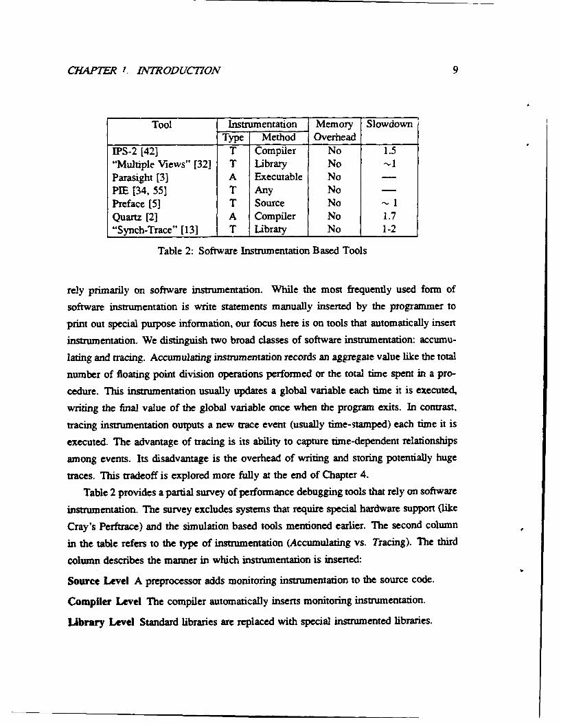
Tool Instrumentation Memory SlowdownType Method Overhead
IPS-2 [42) T Compiler No 1.5"Multiple Views" [32] T Ubrary No --1Parasight [3) A Executable NoPIE [34, 55] T Any NoPreface [5] T Source No -- 1Quartz [2) A Compiler No 1.7"Synch-Trace" [13) T Library No 1-2
Table 2: Software Instrumentation Based Tools
rely primarily on software instrumentation. While the most frequently used form of
software instrumentation is write statements manually inserted by the programmer to
print out special purpose information, our focus here is on tools that automatically insert
instrumentation. We distinguish two broad classes of software instrumentation: accumu-
lating and tracing. Accumulating instrumentation records an aggregate value like the total
number of floating point division operations performed or the total time spent in a pro-
cedure. This instrumentation usually updates a global variable each time it is executed,
writing the final value of the global variable once when the program exits. In contrast,
tracing instrumentation outputs a new trace event (usually time-stamped) each time it is
executed. The advantage of tracing is its ability to capture time-dependent relationships
among events. Its disadvantage is the overhead of writing and storing potentially huge
traces. This tradeoff is explored more fully at the end of Chapter 4.
Table 2 provides a partial survey of performance debugging tools that rely on software
instrumentation. The survey excludes systems that require special hardware support (like
Cray's Perftrace) and the simulation based tools mentioned earlier. The second column
in the table refers to the type of instrumentation (Accumulating vs. Tracing). The third
column describes the manner in which instrumentation is inserted:
Source Level A preprocessor adds monitoring instrumentation to the source code.
Compiler Level The compiler automatically inserts monitoring instrumentation.
Library Level Standard libraries are replaced with special instrumented libraries.
CHAPTER 1. INTRODUCTION 10
Executable Level The executable program is patched to add instrumentation.
The instrumentation method can have some impact on user convenience as it determines
whether or not recompilation is necessary. The fourth column of the table refers to the
ability of tools to distinguish memory overhead from compute time, and the last column
provides information on the ratio of the execution times of instrumented and raw versions
of a program. A dashed line in the table indicates that no details about overhead were
reported.
We note two important trends in the table. First, none of software-based tools distin-
guishes memory overhead from compute time. Second, several descriptions of tools either
ignore instrumentation overhead or report overheads in excess of 50%. The two articles
that report negligible instrumentation overhead, Multiple Views and Preface, both add the
caveat that overhead is proportional to task granularity and frequency of synchronization.
This caveat applies generally to software instrumentation. When the monitoring
instrumentation does not directly effect the monitored events and these events occur
infrequently, the perturbation introduced by monitoring is typically small and acceptable.
For example, for loosely coupled parallel programs with coarse tasks that synchronize
infrequently, it is reasonable to generate a time-stamped event on each synchronization
object acquisition/release and message send/receive. Examining the trace-based systems
in Table 3, we observe that the two tools with the least overhead, Multiple Views and
Preface, each instrument only coarse synchronization events. The Synch-Trace study
also traces only synchronization events, but one of the monitored programs synchronizes
frequently and the instrumentation slows that program by 100%. IPS-2 generates events
on procedure entry and exit as well at synchronization points so its overhead depends on
the rate at which procedures are called, varying from negligible overhead for programs
with large procedures to more than 50% for a recursive sort program. In general, the low
overhead of the trace-based systems in Table 3 derives from on the fact that they trace
infrequent, coarse-grained events. This assumption does not, however, apply to memory
access events.
The drawback of software instrumentation is its potential to distort execution behav-
ior so much that the data collected is irrelevant to the performance of the original code.
Instrumentation can easily affect memory system performance, for example changing
CHAPTER 1. INTRODUCTION 11
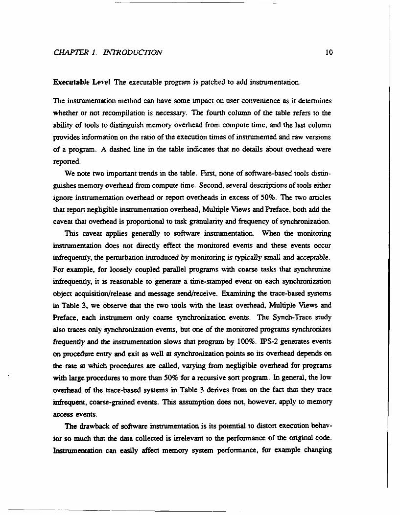
Technique Advantages Drawbacks
Static Analysis Fast; Can be implemented Limited applicabilityin compiler
Simulation Arbitrarily precise Slow
Hardware Non-intrusive, fine-grained Difficult to relate hard-Instrumentation ware events to programmer
level; Not widely available
Software Fast, flexible Fails to capture memoryInsmtrnentation behavior; Intrusive
Table 3: Summary of Performance Debugging Approaches
instruction cache behavior or altering peak data bandwidth requirements. In addition,
because instrumentation inevitably alters the timing of the program, it distorts synchro-
nization behavior. Thus, it is not clear that we can trust the data collected by tools that
rely on software instrumentation. This problem is explored more fully in Chapter 3.
1.3 Scope and Contributions
Table 3 summarizes our survey of techniques for gathering performance information. Our
goal is to build a performance debugging tool that is fast enough to allow the programmer
to experiment with many different program implementations and accurate enough to show
him where and how execution time is being spent. Weighing the tradeoffs among the
various approaches, it seems that software instrumentation would be ideal if not for its
potential intrusiveness and inability to detect memory system overhead. This dissertation
offers ways to overcome these two drawbacks. Our approach is to use basic block count
profile information both to control intrusiveness and to isolate memory system overhead.
Lightweight instrumentation is used to collect selected branch execution counts and more
extensive off-line analysis produces a full basic block count and memory overhead profile.
(A basic block is a contiguous set of instructions with unique entry and exit points.)
Our first step is to instrument a program by placing a counter in front of each basic
block. Using a knowledge of instruction latencies and the basic block counts obtained by

CHAPTE 1. INTRODUCTION 12
running the instrumented program, we can build an ideal compute time profile describing
how much time the program spent in each basic block. This profile is used both to
identify important regions of the program to instrument with performance probes and to
insure that the overhead of such probes is kept to acceptable levels (on average less than
10%).
Guided by the initial profile information, we instrument a program to collect two
kinds of information: actual time spent in selected loops, procedures, and synchroniza-
tion calls, and basic block counts. Memory losses can be isolated by comparing the
actual time measurements to compute time estimates made using the basic block counts
under the assumption of an ideal memory system. Synchronization overheads can be
identified directly from execution time measurements of synchronization calls. Finally,
extra work can be estimated using instruction count information whenever either the user
tags instructions as "extra work" or we can recognize instructions as extra work because
they occur in parallel control constructs. Thus, by combining the ideal compute time
profile derived from basic block counts with an actual user time profile, we can derive
integrated information on sources of performance loss.
This dissertation demonstrates the effectiveness of an integrated software instrumen-
tation approach. Chapter 2 introduces a simple tool, Mprof, which isolates memory
overhead in sequential programs. Mprof is used to characterize the SPEC benchmark
suite. The information from Mprof leads to substantial improvements in memory system
performance in three of the benchmarks. Chapter 3 addresses the problem of controlling
the overhead of instrumentation. We offer the basic block profile as a powerful tool
for controlling perturbation. Suppose, for example, that we are considering adding in-
strumentation that executes in T cycles to a certain basic block. Multiplying T by the
number of times the basic block executes gives an estimate of the overhead that will be
introduced by the instrumentation. This estimate allows us to make an informed decision
as to whether or not to insert the instrumentation. Chapter 3 exploits this observation to
develop a simple algorithm for reduced cost basic block counting. Chapter 4 combines
the memory overhead detection technique and low cost instrumentation of the previous
two chapters and introduces a new multiprocessor performance debugging tool called
Mtool. Mtool augments a program with low overhead instrumentation which perturbs

CHAPTER 1. INTRODUCTION 13
the program's execution as little as possible while generating enough information to iso-
late memory and synchronization bottlenecks. After running the instrumented version
of the parallel program, the programmer can use Mtool's window-based user interface
to view compute time, memory, and synchronization bottlenecks at increasing levels of
detail from a whole program level down to the level of individual procedures, loops and
synchronization objects. Chapter 4 also describes Mtool's attention focusing mechanisms
and compares them with other approaches. Finally, Chapter 5 validates our software
instrumentation approach, offering several case studies that demonstrate Mtool's effec-
tiveness. Chapter 6 offers conclusions and suggests directions for further research.
Chapter 2
Detecting Memory Overhead in
Sequential Code
This chapter presents a new method for detecting regions of a program where the memory
hierarchy is performing poorly. By observing where actual measured execution time dif-
fers from the time predicted given an "ideal" memory hierarchy, we can isolate memory
system overhead. The chapter consists of four sections. The first shows how to derive an
ideal compute time profile using basic block count information and an accurate pipeline
model. The second describes Mprof, a tool that isolates memory system overhead at the
level of loops and procedures by comparing an ideal compute time profile with actual
execution times gathered using pc-sampling. To explore Mprof's strengths and weak-
nesses, we apply it to the ten SPEC benchmarks. For each SPECmark, we quantify the
memory overhead and either modify the code to improve its memory system performance
or discuss why the memory overhead is difficult to remove. In several cases, Mprof fails
to isolate the exact source of memory system overhead because the coarse resolution of
100HZ pc-sampling precludes accurate measurement of individual procedure execution
times. The final two sections address this problem, explaining how to instrument code
to collect actual time profiles by explicitly reading high resolution clocks.
14
CHAPTER 2. DETECTING MEMORY OVERHEAD iN SEQUENTIAL CODE 15
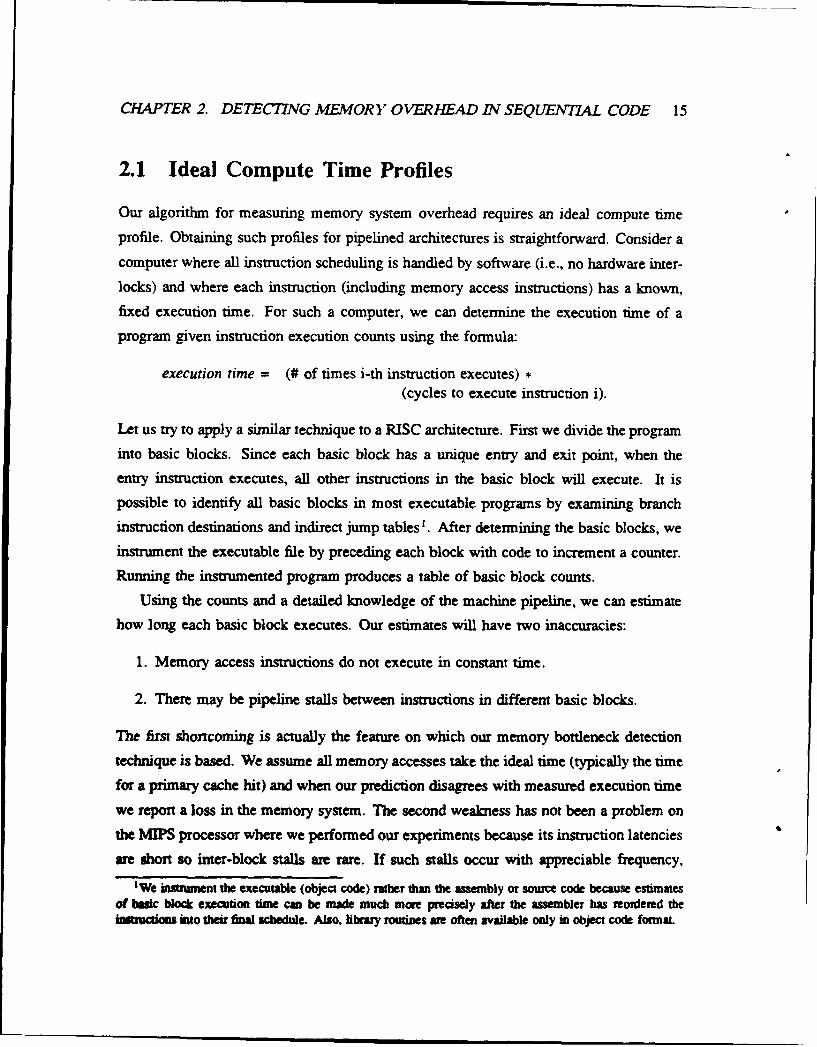
2.1 Ideal Compute Time Profiles
Our algorithm for measuring memory system overhead requires an ideal compute time
profile. Obtaining such profiles for pipelined architectures is straightforward. Consider a
computer where all instruction scheduling is handled by software (i.e., no hardware inter-
locks) and where each instruction (including memory access instructions) has a known,
fixed execution time. For such a computer, we can determine the execution time of a
program given instruction execution counts using the formula:
execution time = (# of times i-th instruction executes) •(cycles to execute instruction i).
Let us try to apply a similar technique to a RISC architecture. First we divide the program
into basic blocks. Since each basic block has a unique entry and exit point, when the
entry instruction executes, all other instructions in the basic block will execute. It is
possible to identify all basic blocks in most executable programs by examining branch
instruction destinations and indirect jump tables'. After determining the basic blocks, we
instrument the executable file by preceding each block with code to increment a counter.
Running the instrumented program produces a table of basic block counts.
Using the counts and a detailed knowledge of the machine pipeline, we can estimate
how long each basic block executes. Our estimates will have two inaccuracies:
1. Memory access instructions do not execute in constant time.
2. There may be pipeline stalls between instructions in different basic blocks.
The first shortcoming is actually the feature on which our memory bottleneck detection
technique is based. We assume all memory accesses take the ideal time (typically the time
for a primary cache hit) and when our prediction disagrees with measured execution time
we report a loss in the memory system. The second weakness has not been a problem on
the MIPS processor where we performed our experiments because its instruction latencies
are short so inter-block stalls are rare. If such stalls occur with appreciable frequency,
'We insument the executable (object code) rather than the assembly or source code because estimatesof basic block execution time can be made much more precisely after the assembler has reordered the
actions into their &aW schedule. Also, library routines are often available only in object code format.
CHAPTER 2. DETECTING MEMORY OVERHEAD IN SEQUENTIAL CODE 16
they can be accounted for by instrumenting to collect branch frequencies as well as basic
block counts. The branch frequencies tell us how often one basic block precedes another
and we can improve our estimate by including stalls between adjacent basic blocks. Thus,
we have a technique for estimating the ideal compute time of groups of basic blocks.
2.2 Isolating Memory Overheads with Mprof
On UNIX systems the prevalent technique for collecting an actual time profile is pc-
sampling. The operating system periodically interrupts a program and increments a
counter corresponding to the region containing the current program counter (pc). The
sampling rate is typically 60-100HZ and the impact of sampling on program performance
is small as UNIX is already stopping the process regularly in order to maintain the system
software clock.
Mprof gathers its actual time profile by using the UNIX pc-sampling facility with
one counter for each instruction in the profiled program. Mprof instruments the program
to call profil when execution begins and to write the array of sampled counts to a
file when the program exits. Mprof's instrumentation is inserted either by augmenting
the source code with calls to begin and end profiling or by replacing the standard li-
brary start and .exit routines with instrumented routines (i.e., linking with a special
libcrt0.a as is done in PROF).
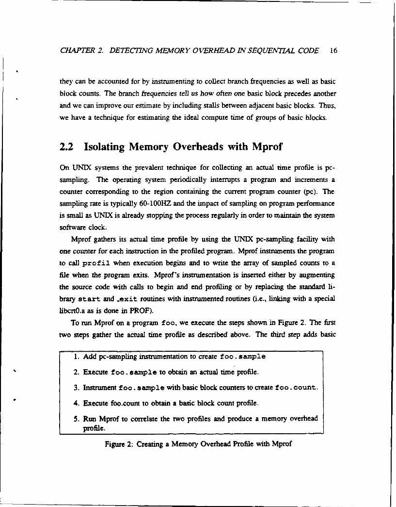
To run Mprof on a program foo, we execute the steps shown in Figure 2. The first
two steps gather the actual time profile as described above. The third step adds basic
1. Add pc-sampling instrumentation to create foo. sample
2. Execute foo. sample to obtain an actual time profile.
3. Instrument foo. sample with basic block counters to create foo. count.
4. Execute foo.count to obtain a basic block count profile.
5. Run Mprof to correlate the two profiles and produce a memory overheadprofile.
Figure 2: Creating a Memory Overhead Profile with Mprof

CHAPTER 2. DETECTING MEMORY OVERHEAD IN SEQUENTIAL CODE 17
block counting instrumentation. On MIPS-processor based systems, the PIXIE profiler
(provided with the system by MIPS) will accomplish this step by instrumenting the
executable. The final step isolates memory overhead by correlating the actual execution
time and basic block count profiles.
Note the Mprof sequence involves running foo twice, once to gather each profile.
One might consider collecting both the actual time profile and the basic block count
profile in a single execution of the program (i.e., skipping step 2). The problem with
accumulating both profiles simultaneously is that the actual time profile will include the
time spent executing the basic block counting instrumentation. To recover an actual time
profile for the raw program, we must factor out the effects of the counter instrumentation.
Since Mprof is intended for use with sequential programs, it can avoid the complexity of
compensating for counter instrumentation by collecting its profiles in two separate runs
that are assumed to be comparable. However, in a parallel programming environment,
the problem of simultaneously collecting profiles must be addressed because two runs of
a program on a single input may not be directly comparable; the issue is discussed at
length in Chapter 3.
Given basic block count and pc-sample profiles, for any group of basic blocks in the
program Mprof can compute three values:
Compute Time = Xbasic blocks b (# times b entered) * (b's ideal compute time)
Actual Time = -instructions i (pc-sampled time for i)
Memory Overhead = Actual Time - Compute Tune
The final equation is our definition of memory overhead. Note, this definition does not
refer to the cause of the memory overhead: it may be cache interference, TLB misses, bus
contention, write buffer stalls, etc. However, we have found that isolating and quantifying
memory system effects at the loop and procedure level often allows a trained programmerto deduce why the overhead is arising.
To support this claim, we present and analyze the Mprof memory overhead profile
for each benchmark in the SPEC suite. Mprof produces a profile by using the equations
above to derive memory overhead for the whole program and for each procedure withinthe program. If actual time for a procedure is less than 0.5 seconds, Mprof ignores
the procedure as pc-sampling at 100HZ seems accurate to about 0.1 seconds and Mprof

CHAPTER 2. DETECTING MEMORY OVERHEAD IN SEQUENTIAL CODE 18
CPU Utilization 77.0% (Actual Time 55.1 sec. vs Compute Time 42.4)PROCEDURE NAME % Actual Time Time in Sec. CPU
Net Mem Corn Mem Com Utilcmppt 85.4 18.7 66.7 10.3 36.7 78.0
Loop from 43 to 57 78.4 13.7 64.7 7.5 35.6 82.5..dopmt 3.6 1.3 2.3 0.7 1.2 63.3
Loop from 301 to 991 2.0 0.4 1.6 0.2 0.9 78.0Loop from 301 to 991 2.0 0.5 1.6 0.3 0.9 76.3
Loop from 974 to 978 0.8 0.4 0.3 0.2 0.2 42.4
Figure 3: Mprof output for eqntott
is designed to avoid reporting spurious memory overheads 2. Mprof sorts procedures
in decreasing order of memory overhead, selecting those procedures that account for
97% of all memory overhead for further analysis. For each selected procedure, Mprof
identifies loops in the control flow graph, and computes memory overhead for each loop
in the procedure. The line number information in the executable is then used to relate
the compute time and memory overhead information for the loops and procedures in
the object code back to the source code. A sample Mprof output file for the eqntott
program from the SPECmarks is shown in Figure 3.
The top line of the figure gives a whole program profile summary. The CPU utilization
metric is defined as:Compute Time
Compute Tune + Memory Overhead
We find that eqntott had a CPU utilization of 77%. The profile provides data on the
memory overhead and ideal compute time for various procedures and loops, both as a
percentage of total execution time and as absolute time in seconds. Procedures are listed
in the profile in decreasing order of memory overhead to highlight memory bottlenecks.
The first entry tells us that 18.7% of execution time was spent waiting on the memory
hierarchy in the cmppt procedure; memory overhead in the loop of lines 43 to 57 in this
2Th accuracy of pc-sampling depends on the arrival of the sampling interrupt being uncorrelated withthe program execution. This lack of correlation is difficult to guarantee, so it is hard to construct a reliablegeneral bound on the accuracy of pc-sampling. Extensive testing has shown the 0.1 second figure to be alower bound for our programs on UNIX systems.

CHAPTER 2. DETECTING MEMORY OVERHEAD iN SEQUENTIAL CODE 19
Program CPUName Util.
matrix300 25.5dnasa7 30.9spice2g6 46.3tomcatv 48.0gcc (ccl) 51.1xlisp 76.3eqntott 77.0doduc 77.3
fpppp 79.5espresso 91.8
Table 4: CPU Utilizations of the SPECmarks
procedure accounts for 13.7% of all program execution time. When entries in the tablerefer to loops, the level of indentation of the word "Loop" corresponds to nesting depth.
Appendix A gives full MPROF listings for each of the SPECmarks when compiled
with 02 optimization on an SGI 4D/380 running IRIX 4.0. The SGI 4D/380 has a
two level cache: the primary cache is 64KB direct-mapped with 16 byte lines and the
secondary cache is 256KB, direct-mapped, with 64 byte lines. Table 4 summarizes
the CPU utilizations for the SPECmarks. Examining the table, we find that half the
programs have better than 75% CPU utilization; the five remaining codes spend 50%
to 75% of their execution time waiting on the memory hierarchy. For three of these
five programs, matrix300, tomcatv, and nasa7, Mprof highlights loops where memory
performance enhancing transformations are relatively straightforward to apply. In theremaining two cases, spice and gcc, reducing memory overhead seems more challenging.
Matrix300 claims the dubious honor of worst sustained CPU utilization among theSPECmarks. The program executes a series of double precision 300x300 matrix mul-
tiplies with only 26% CPU utilization. This performance is particularly disappointing
because matrix multiply involves O( o3) operations (including O( 113) memory references)
but only 0(072) actual operands. Thus, one would expect significant data reuse and goodperformance for processors with cache. However, since the SGI machine's cache is too
CHAPTER 2. DETECTING MEMORY OVERHEAD IN SEQUENTIAL CODE 20
DO 4 J = 2,JJU-JLJX = JU-JDO 15 K = KL,KU
F(JX,K,1) = F(JX,K,1) - X(JX,K)*F(JX+1,K,1)-& Y (JX, K) *F (JX+2, K, 1)
F(JX, K,2) = F(JX,K,2) - X(JX,K)*F(JX+1,K,2)-& Y (JX, K) *F (JX+2, K, 2)
F(JX, K,3) = F(JX, K,3) - X(JX, K) *F (JX+1,K, 3)-& Y (JX, K) *F (JX+2, K, 3)
15 CONTINUE4 CONTINUE
Figure 4: A Critical Loop in vpenta
small to store the full matrices that are being multiplied, the reuse can only be utilized if
we block the computation. A careful study of the issues involved in optimizing matrix
multiply for direct mapped caches can be found in [31]. In general, manufacturers or
third-party vendors usually supply optimized BLAS3 library implementations of basic
linear algebra routines that have been blocked to take advantage of machine-specific
memory hierarchy characteristics. Using such a routine optimized for the SGI memory
hierarchy reduces total execution time from the 338 seconds of the raw SPECmark to
about 48 seconds, with CPU utilization climbing from 26% to 83%3.
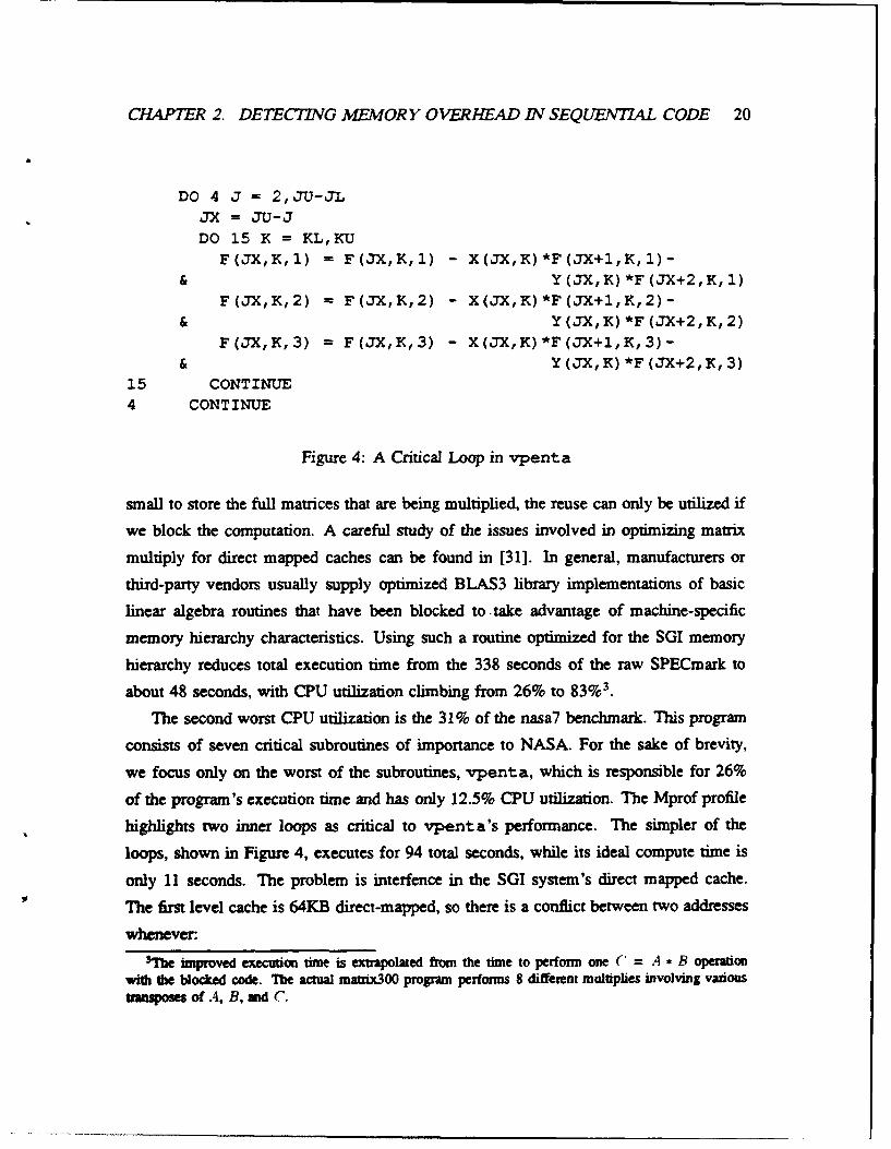
The second worst CPU utilization is the 31% of the nasa7 benchmark. This program
consists of seven critical subroutines of importance to NASA. For the sake of brevity,
we focus only on the worst of the subroutines, vpenta, which is responsible for 26%
of the program's execution time and has only 12.5% CPU utilization. The Mprof profile
highlights two inner loops as critical to vpenta's performance. The simpler of the
loops, shown in Figure 4, executes for 94 total seconds, while its ideal compute time is
only 11 seconds. The problem is interfence in the SGI system's direct mapped cache.
The first level cache is 64KB direct-mapped, so there is a conflict between two addresses
whenever.
3•re improved execution time is extrapolated from the time to perform one C = A * B operationwith the blocked code. The actual matix300 program performs 8 different multiplies involving various
poses of .4, B, and C.
CHAPTER 2. DETECTING MAIMORY OVERHEAD EV SEQUENTIAL CODE 21
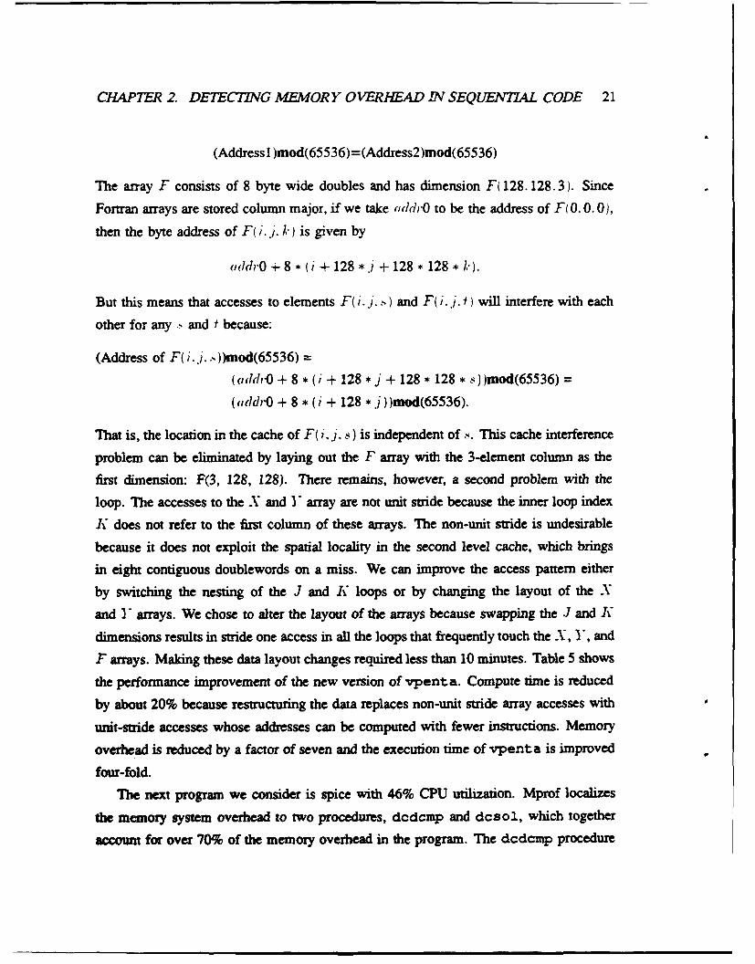
(Address I )mod(65536)=(Address2)mod(65536)
The array F consists of 8 byte wide doubles and has dimension F( 128.128.3). Since
Fortran arrays are stored column major, if we take addrO to be the address of F{ 0.0.0),
then the byte address of F( i. j..k) is given by
(ddrO + 8 * (i + 128 * .i + 128 , 128 * k).
But this means that accesses to elements F( i. j.O ) and F( i.J.. •) will interfere with each
other for any .! and f because:
(Address of F( i.1. .))mod(65536)(add,'O + 8 * (i + 128 *j + 128 * 128 * .,))mod(65536) -
(addrO + 8 * (i + 128 * j))mod(65536).
That is, the location in the cache of F( i .j.. s) is independent of .. This cache interference
problem can be eliminated by laying out the F array with the 3-element column as the
first dimension: F(3, 128, 128). There remains, however, a second problem with the
loop. The accesses to the X and Y" array are not unit stride because the inner loop index
K does not refer to the first column of these arrays. The non-unit stride is undesirable
because it does not exploit the spatial locality in the second level cache, which brings
in eight contiguous doublewords on a miss. We can improve the access pattern either
by switching the nesting of the J and K loops or by changing the layout of the X
and Y arrays. We chose to alter the layout of the arrays because swapping the J and K
dimensions results in stride one access in all the loops that frequently touch the X, Y, and
F arrays. Making these data layout changes required less than 10 minutes. Table 5 shows
the performance improvement of the new version of vpenta. Compute time is reduced
by about 20% because restructuring the data replaces non-unit stride array accesses with
unit-stride accesses whose addresses can be computed with fewer instructions. Memory
overhead is reduced by a factor of seven and the execution time of vpenta is improved
four-fold.
The next program we consider is spice with 46% CPU utilization. Mprof localizes
the memory system overhead to two procedures, dcdcmp and dcsol, which together
account for over 70% of the memory overhead in the program. The dcdcmp procedure

CHAPTER 2. DETECTING MEMORY OVERHEAD IN SEQUENTIAL CODE 22
Util Compute Memoryvpenta.orig 12.6 35.8 248.9vpenta.new 52.7 29.8 33.2
Table 5: Reducing Memory Overhead in vpenta
performs a sparse LU decomposition with partial pivoting and fill-in control. The routine
has 44% CPU utilization. It is unlikely that simple transformations can improve the
performance of this routine, because the pivoting operation involves a row interchange at
each step. This interchange can substantially alter the structure of the matrix, so standard
techniques for exploiting locality in sparse matrix factorization are not directly applicable.
The dcsol procedure uses the LU decomposition computed by dcdcmp to solve
a system using forward and back substitution. Mprof tells us that memory overhead
in dcsol is responsible for 7% of whole program execution time and the procedure
has 31% CPU utilization. Again, however, this poor memory hierarchy performance is
difficult to avoid; there is little reuse of data in the forward and back solve algorithm.
For the spice program, Mprof succeeds in isolating and quantifying the memory system
effects, but achieving better memory system performance would require fundamentally
altering the sparse matrix algorithms used by the program.
In contrast, improving on the 48% CPU utilization of tomcatv is simple. Mprof
highlights a single twenty four line loop as the source of most of the memory system
overhead. Examining the source code, we find the loop makes stride one access to the
elements of two arrays X and 3'. In fact, Y(i.j) is read every time X(0.j) is read.
Because the accesses are stride one and the CPU utilization is poor, our hypothesis is
that the arrays have been stored in such a way that X(i.j) often conflicts with Y(i.j).We check this hypothesis by changing the layout of Y:
DIMENSION X(N,N),Y(N,N) •DIMENSION X(N,N), Y(N+7,N).
Modifying the first dimension of 3' alters the relative mapping of X and Y which should
decrease cache interference between the arrays. Running the modified code, we find
compute time is unchanged while total execution time is improved by roughly a third
CHAPTER 2. DETECnNG MEMORY OVERHEAD IN SEQUENTIAL CODE 23
from 172 seconds to 123 seconds. Mprof has highlighted memory overhead that was
easily reduced.
The final SPECmark with poor memory behavior is gcc with 51% CPU utilization.
Examining the raw data in Appendix A, it is apparent that Mprof attributes only 21%
of total program time to memory overhead in particular procedures. An additional 30%
of execution time is reported as memory overhead, but the constraint that pc-sampled
procedure times are accurate only when they exceed 0.5 seconds prevents Mprof from
isolating which specific procedures account for this overhead. The next section addresses
this problem, discussing techniques for using high resolution clocks to gather finer grained
actual time profile information.
The remaining five SPECmarks all have CPU utilizations of 75% or better. For
these programs, even a factor of two reduction in memory overhead will improve whole
program performance by less than 13%. Thus, the programmer's effort is probably better
expended in trying to make actual computation more efficient. At the end of Appendix A,
we explore this hypothesis by examining the Mprof profile of each of the five programs
that spend less than 25% of execution time waiting on the memory hierarchy. For each
program, we give a qualitative assessment of the amount of effort required to reduce this
overhead.
In summary, this section offered a tool, Mprof, which isolates memory overhead by
comparing ideal and actual execution times. Applying Mprof to the SPECmarks on a
single processor SGI system, we found five of the benchmarks have 75% or better CPU
utilization, three benchmarks have memory overheads that can be easily reduced, and
two programs have significant memory overhead that is either inherent in the algorithms
or difficult to pinpoint.
2.3 Better Clock Resolution
Table 6 provides data on the total number of lines in the source code associated with the
memory overheads that Mprof isolated. The entries in the table were computed from the

CHAPTER 2. DETECTING MEMORY OVERHEAD 1N SEQUENTIAL CODE 24
Program CPU Total # of Source LinesName Util. Lines 50% 75% 90%
mr.rix300 25.5 439 2 2 2dnasa7 30.9 1105 17 28 46spice2g6 46.3 18411 27 69 613tomcarv 48.0 198 25 29 39gcc (ccl) 51.1 54182 - - -
xlisp 76.3 7413 78 168 317eqntont 77.0 2763 15 26 -
doduc 77.3 5334 413 1538 -
fpppp 79.5 2718 411 1109 1690espresso 91.8 46498 - - -
Table 6: Lines of Source Code vs. Percentage of Total Memory Overhead
Mprof profiles by associating a memory overhead per line,
Overhead in Seconds In Loop or Procedure# of Lines in Loop or Procedure
with each item in the profile, sorting by memory overhead per line, and selecting those
loops and procedures that account for the first 50%, 75% and 90% of all memory over-
head. Missing entries in the table correspond to programs where Mprof failed to isolate
a certain percentage of memory overhead: Some procedures were ignored because the
timing resolution of pc-sampling is limited.
For gcc and espresso, Mprof attributes less than half of all memory overhead to
specific procedures. On the other hand, for each of the four loop-intensive scientific
programs, Mprof localizes at least half of the memory overhead to 27 or fewer lines of
source code. In general, the straightforward Mprof implementation based on pc-sampling
is accurate in pinpointing memory overhead in scientific code, but its effectiveness is more
limited in general purpose modular code which is broken into many short procedures.
Ideally, Mprof would accurately measure actual aggregate execution time for each
memory access instruction (e.g. load or store) in the executable program. Then, memory
overhead could be isolated at the level of the particular instruction that caused it. This
ideal measurement scheme is difficult to achieve in practice. The missing entries in

CHAPTER 2. DETECTING MEMORY OVERHEAD IN SEQUENTIAL CODE 25
Table 6 show that pc-sampling is already too crude to accurately measure the time spent
in many procedures; much greater resolution would be needed to time individual memory
access instructions.
One alternative that offers better resolution is hardware clocks. We categorize hard-
ware clocks by their accuracy and the overhead involved in accessing them. Some
processors like the CRAY, HP Precision, IBM RS6000, and MIPS R4000 provide a high
resolution cycle counting register directly accessible to the processor so clock accuracy
is excellent and overhead is small. Commonly, however, a relatively high resolution
clock is available, but it requires more extensive overhead to access. For example, SGI
multiprocessors include a 16MHz cycle counter on the Ethernet/IO board. The clock
is directly addressable by user processes, but reading it involves going up the memory
hierarchy and over the shared bus. For a global clock, this overhead is difficult to avoid
because a value that changes 16 million times per second cannot be kept in cache.
Let us consider how we can use high resolution timers to isolate memory bottlenecks.
We call a set of instructions in which we can identify all entry and exit points a measurable
object or m-object. The object is measurable because we can place start timer and stop
timer calls at the entry and exit points to measure the time spent in the object. For
example, we can time a procedure by placing a start.timer call at the top of the procedure
and stop-timer calls before every return statement. Similarly, we can time a loop by
placing a start-timer above the top of the loop and a stop.timer below the bottom of the
loop.
We say an m-object is timable if we can instrument the program to measure the time
spent within the object. A timable object must satisfy two criteria:
"* The total time spent within the object substantially exceeds timer granularity.
"* The perturbation introduced by reading the clock is acceptably small.
Perturbation has two aspects. To avoid changing memory performance, we require that
the number of memory operations performed by the m-object substantially exceed the
number performed in a clock timer call. In addition, to avoid appreciably slowing the
program down, we require that the time spent in the m-object is much greater than the
time to make a clock call.

CHAPTER 2. DETECTING MEMORY OVERHEAD IN SEQUENT7AL CODE 26
1. Instrument foo with basic block counters and execute it to gather a profile.
2. Use the profile to select those basic blocks responsible for 98% of all mem-ory operations.
3. For each selected basic block, select the loops (if any) and procedure thatcontain the block.
4. Eliminate any selected m-objects that are not timable.
5. For each selected basic block, select the smallest remaining estimable m-object. Instrument to time all selected m-objects.
6. Run the instrumented code and correlate the estimated and actual time pro-files to isolate memory overheads.
Figure 5: Using Explicit Clock Reads with Mprof
Using the above criteria, we can identify regions of the program whose actual exe-
cution times can be measured. These execution times include, however, both the work
done in an m-object proper and the work done on behalf of the object by any procedures
that it calls. In contrast, the technique for estimating ideal compute time described in
Section 2.1 calculates only the work done in a basic block; it ignores ideal compute time
spent in procedure calls. Furthermore, while we can estimate the total compute time
spent in a procedure q, we cannot necessarily determine the compute time spent in q on
behalf of a particular caller. Thus, we cannot always estimate the time spent in and on
behalf of an m-object that calls q. We will say that the m-objects whose execution time
can be accurately predicted by basic-block counting techniques are estimable.
We can isolate a memory bottleneck whenever an m-object is both timable and es-
timable. Figure 5 describes an implementation of Mprof that gathers actual time infor-
mation using explicit clock reads instead of pc-sampling. The first three steps utilize an
initial basic block count profile to identify a set of potential m-objects. Step 4 is imple-
mented by using the basic block count profile to verify the timability of each m-object.
For each m-object, we derive an ideal compute time that provides a lower bound on the
actual execution time of this m-object. The lower bound allows us to check that the
clock resolution is adequate to accurately measure the time spent in the m-object. To

CHAPTER 2. DETECTING MEMORY OVERHEAD IN SEQUENTIAL CODE 27
check the second aspect of timability, namely perturbation, we use the basic block count
information to estimate the overhead introduced by a timer:
(overhead for timer instrumentation) , (# of times the m-object is entered)
If the overhead exceeds a specified bound, the m-object is rejected as untimnable.
Implementing the estimability check of Step 5 is more complex. If the m-object does
not contain any procedure calls, it is immediately estimable. If it does make calls, the
simplest approach is to place timers around any calls and subtract off the time spent in
them. This approach is not always applicable, however, as the overhead of reading the
clock can be substantial compared to the time spent in the call. For example, the absolute
value library routine fabs on the SGI machine executes in about 10 cycles while the
overhead of reading the off-processor hardware cycle counter twice to time the f abs
call is around 60 cycles. This six-fold slowdown seems unacceptable.
The simplest alternative to timing off the effect of calls is verifying estimability using
information about the structure of a program's call graph. In a call graph, nodes represent
procedures and there is a directed edge from node v, to node w if procedure v calls w
during the execution of the program. The call graph has a distinguished node, the root,
which is the procedure where execution begins. We say a node v dominates W, if every
path through the graph from the root to w passes through v. A useful observation about
the call graph is that a node is estimable if it dominates all of its descendants. Intuitively,
if a node v dominates w then all the work in w is done on behalf of v. Hence, if a node
dominates all of its children, then the estimated time for that node and its descendants is
just the sum of each of their estimated times, ignoring procedure calls. Using a simple
depth first traversal, it is straightforward to check that a node in the call graph dominates
all of its descendants. It is easy, therefore, to verify that the procedure corresponding to
the node is estimable. However, because many procedures have multiple callers, many
nodes do not dominate all of their descendants and this estimability check will fail.
When the check does fail, we must apply other techniques to verify that average ideal
compute time per call from an m-object to a procedure p is accurately approximated by
the average ideal compute time for p. For example, many scientific library routines are
simple, loop-free leaf procedures that always follow the same execution path. Their esti-
mated execution times are consequently constant. We can often identify such procedures

CHAPTER 2. DETECTING MEMORY OVERHEAD IN SEQUENTIAL CODE 28
by checking that they meet two conditions:
1. The procedure is loop-free and call-free.
2. The average time per call as determined by basic block counts is equal to themaximum or minimum possible time per call.
The first condition implies the procedure is estimable and that we can run shortest and
longest path algorithms on the control flow graph of the procedure to bound its execution
time. Using these bounds, we can check the second condition which implies that the
execution time per call is constant because average equals extremum. This test finds that
such common library calls as sqrt and exp have constant execution times when called
in the Perfect Club benchmarks.
A final heuristic that is often useful when we can neither time off the efftcts of a
procedure call, nor prove that it is safe to use average time per call, is to check whether
the error introduced by using average time per call is small. If an m-object r calls p and
(avg. time per call to p)*(# of calls from 2- to p) < time spent in r
then the error introduced by the average time approximation should be negligible. Of
course, under pathological conditions when the variance in execution time of p is large
and correlated with the call site, this approximation can fail, so Mprof must issue a
warning when it is used.
An alternative approach to avoiding problems with estimability is to use special
basic block counting instrumentation to accumulate counts on a per call site basis for
selected procedures. One obvious method is linkage tailoring to create unique copies of
a procedure body for particular call sites. A second approach is to use instrumentation
that increments call site specific counters. For example, if accesses to counters are
implemented using indirection off a base register and the value of the base register does
not change within the called procedure, then the caller to the procedure can alter the base
register to point to a set of call site specific counters.
Thus, Mprof can choose from a wide variety of techniques to enforce the estimability
condition in Step 5 of our algorithm. Once Mprof identifies timable, estimable m-objects,
it can instrument them with timers and collect a high resolution actual time profile. An
CHAPTER 2. DETECTING MFMORY OVERHEAD IN SEQUENTIAL CODE 29
early implementation of Mprof that used explicit timer readc is described in some detail
in [21]. Because no hardware clock was available, that system used a low-precision, low-
overhead software clock. Despite this limitation, experience with the system demonstrated
that the initial basic block count profile nearly always provides enough information for
simple heuristics to automatically select a reasonable set of rn-objects for low overhead
instrumentation. In the cases where the heuristics fail, the user was given the option to
override them.
2.4 Effectiveness of High Resolution Clocks
We have just described a method for collecting actual time profile data using explicit
timer calls rather than pc-sampling. The natural question is: How much is gained by
using the higher resolution clock? Ideally, we would like to quantitatively contrast theprecision with which the two profiling techniques isolate memory overhead. In particular,
we would like to compare the number of lines of source code associated with 90% of
memory overhead in Mprof profiles generated using each of the actual timing methods.We cannot address this question directly because Mtool has yet to be ported to a
system with a high resolution, low overhead timer. Instead, we estimate how much
a good clock will improve Mprof's ability to isolate memory overhead to the level of
individual procedures. Examining Table 6 we find that for four of the ten SPECmarks,
Mprof could not identify specific procedures that collectively accounted for at least 90% of
the program's net memory overhead. The pc-sampled profile was too crude to measure
the actual execution times of certain procedures that involve non-negligible memory
overhead.
We now estimate the extent to which a high resolution timer could effectively measure
the actual times spent in the missing procedures. More concretely, we consider an on-
processor free running cycle counter with single cycle resolution and single cycle access
time. Using this counter, we can time a procedure with about 10 cycles of overhead by
reading the counter on procedure entry and exit and updating in memory a running tally
of aggregate time spent in the procedure. We assume Mprof will enforce a heuristic that
uses explicit clock reads to time a procedure only if the average execution time of the

CHAPTER 2. DETECTING MEMORY OVERHEAD IN SEQUENTI4L CODE 30
O-100 - rw exat time
ccc eqn dod eC Benchmarg
0
40-
20.
01- - - -9CC *qf dod esp
Benchmark
Figure 6: Improvement in Memory Operation Coverage
procedure is at least 100 cycles (so overhead is at most 10%).
Figure 6 plots the percentage of dynamically executed memory operations that will
be measured in specific procedures with pc-sampling alone and with pc-sampling supple-
mented by high-resolution timers. While memory operation coverage does not correspond
exactly to memory overhead coverage, it still provides a useful approximation. For gcc,
the explicit timers increase memory operation coverage from 56% to 78% while for
espresso the coverage is improved from 84% to 94%. For the remaining two programs,
eqntott and doduc, explicit clocks reads bring memory operations coverage to nearly
100%.
Not only can high-resolution timers be used to measure actual times in procedures, but
they may also be useful for decreasing the granularity of m-objects from full procedures
and loops to smaller groups of basic blocks. However, reporting overhead results at this
level is problematic for two reasons:
I. In the best case, Mprof would separately time each basic block; however, realisti-
cally timer overhead would be prohibitive for many programs where basic blocks
are 5-10 instructions. Instead, Mprof would need heuristics that start with each
basic block in a procedure as a distinct m-object and then coalesce adjacent pairs

CHAPTER 2. DETECTING MFMORY OVERHEAD IN SEQUENATIAL CODE 31
of m-objects until a set of timable m-objects is obtained.
2. While loops and procedures tend to correspond to objects in the source language,
today's optimizing compilers often produce basic blocks that do not correspond
to any obvious set of lines in the source code. Thus, it is often hard to relate
fine-grained profile information to a user's code.
While these two difficulties are challenging, we believe they can be overcome. For
example, simple heuristics that favor small loops and procedures as m-objects and split
long basic blocks into groups of smaller m-objects will partially solve the first problem.
And, good symbol table support for optimized code should enable us to overcome the
problem of relating basic block level information to user code. In any event, as Figure 6
shows high resolution timers will certainly be helpful for procedure level profiling.
Chapter 3
Reduced Cost Basic Block Counting
The previous chapter showed how Mprof can isolate memory overhead by comparing
actual execution and ideal compute time profiles. Recall that the Mprof implementation
gathers the two profiles in separate runs to avoid the complexity of accounting for effects
the basic block counting instrumentation has on actual execution time. However, as
mentioned earlier, the validity of this two run approach depends upon the assumption
that multiple runs of a sequential program on the same input are directly comparable.
This assumption may not hold for parallel programs. For example, two runs of a
parallel search program may draw tasks from a queue in a slightly different order, resulting
in traversals of vastly different portions of the search space. Without information fromthe programmer, an automatic tool must make the conservative assumption that two runs
of the same parallel program on the same input are not be directly comparable.
Thus, in a multiprocessor environment, if we hope to isolate memory overhead by
comparing ideal and actual execution time, we must gather both profiles in a single
rim. But to use a single run approach, we must solve the problem of accounting for
the effects of the basic block counting instrumentation on the program's actual time
profile. In general, the problem of compensating for perturbation introduced by software
instrumentation is virtually intractable for parallel programs (consider the aforementioned
search program). The obvious goal is to add as little instrumentation overhead as possible.
The first part of the chapter focuses on the problem of reducing the overhead of gathering
basic block counts. A technique is described for augmenting a program with lightweight
32
CHAPTER 3. REDUCED COST BASIC BLOCK COUNTING 33
instrumentation to collect a basic block count profile. The lightweight instrumentation
increasing the execution time of sequential programs by 1-20% as compared with the 4-
200% increases experienced when instrumenting code with the MIPS execution profiler
PIXIE. The technique identifies independent control flow paths, uses an initial profile to
estimate the cost of instrumenting each of the independent paths, and then selects a low
cost set of independent paths for actual instrumentation. At the end of the chapter, we
examine the effects of the same lightweight instrumentation on parallel programs. The
impact of the instrumentation is similar to that for sequential programs slowing execution
by 5 to 22%.
3.1 Controlling Counter Overhead
Interest in fine grained execution profiles that include basic block count and branch
frequency information is growing. For example, optimizing compilers can make use
of such information to enhance register allocation, improve instruction scheduling, and
restructure for better instruction cache behavior [41, 46, 49, 53]. To some extent the
utility of both profile driven optimizing compilers and our memory overhead detection
technique depends on the overhead involved in collecting execution profiles. If for
instance, one could collect a profile with only a 1-5% increase in execution time, it
might be reasonable to leave profiling enabled at all times. One could then accumulate
execution profiles periodically recompiling to reflect the current usage of a program. We
investigate possible approaches to limiting counter overhead below.
Previous work on reducing counter overhead has exploited two observations:
1. If we consider the flow of control of a procedure, it is only necessary to placecounters on independent control paths. Dependent counts can be recovered in apost-processing phase (27, 54].
2. Loops include a built-in counter, the loop index, whose value can be recorded onloop exit thus avoiding the overhead of counting the individual loop iterations (54].
In the 1970's, Knuth exploited the first observation by noting that with minor modifi-
cations, the counts on a procedure's control flow graph satisfy Kirchoff's laws, and thus
the theorems and algorithms associated with these laws can be applied to inexpensively
CHAPTER 3. REDUCED COST BASIC BLOCK COUNTING 34
identify independent control paths and accomplish the post-processing. Our work ex-
pands on Knuth's observation by using profile information about the execution frequency
of each independent control path and knowledge about counter cost to find a minimum
cost set of counters. The technique is explained in detail in Section 3.1.1.
A similar extension of Knuth's algorithm is used in [4] to select independent control
paths for instrumentation with counters. However, in [4] the induction variable optimiza-
tion described in [54] is not exploited, and little attempt is made to limit the number of
instructions used to implement the counters. Thus, the paper does not provide data on
the minimum run-time overhead required to collect an execution profile. In particular,
the overheads reported here are typically a factor of two lower than those in [4].
This section offers a comprehensive study of run-time overhead, assessing the rela-
tive importance of independent control paths, induction variable recognition, and low-cost
counter sequences to overall instrumentation overhead. Following the review of Knuth's
algorithm in Section 3.1.1, we describe in Section 3.1.2 the various type of counters with
which programs can be instrumented: branch taken/fall through counters, basic block
counters, and induction variable edge counters. Section 3.1.3 reports the minimum over-
head we must incur on a MIPS processor when using these counters to record execution
profiles for programs in the SPEC [59] and Stanford SPLASH [58] benchmark suites.
These overheads are derived by using an execution profile to select the cheapest set of
edges to instrument. Our basic conclusion is that the minimum overheads for these pro-
grams range from 1-20% with median overhead around 5.0%. Section 3.1.4 examines
how closely we can approach these ideal overheads using simple heuristics to choose
which edges to instrument. The results with the heuristics are within a factor of two of
those achieved when actual profiles were used to select the best set of edges to instrument
and range from 1-40% with median overhead 9%. The suboptimality of the heuristics is
not surprising, as a heuristic that could select a minimum cost set of labels to measure
would be tantamount to a heuristic that a priori identifies the most frequently executed
paths in a program. Section 3.2 shows that for sequential programs we can compen-
sae for the effects of basic block counting instrumentation by subtracting out the ideal
compute time spent executing instrumentation instructions. Finally, Section 3.3 offers a
summnary and conclusions about controlling basic block counting overhead in sequential

CHAPTER 3. REDUCED COST BASIC BLOCK COUNTING 35
code.
3.1.1 Minimum Overhead Labelling Algorithm
We open this section with an example that illustrates how instrumenting independent
control paths and recognizing induction variables can substantially reduce the cost of
profiling. The latter part of the section provides the formal algorithm for determining a
minimum cost labelling. The technique is actually just a straightforward application of
Kirchoff's first law.
Consider the Fortran subroutine and corresponding control flow graph in Figure 7. In
the graph, there is a node for each basic block and edges represent the flow of control.
Nodes are labelled with basic block counts and edge labels represent the number of times
a path is traversed during the execution of the program. After adding a dummy edge (in
dashes) from the Return node to the Start node and labelling it with the number of times
the procedure is called, the labels on each node and its incident edges must satisfy:
SUBROUTINE FOO(A, B, N)REAL A(N), B(N) STARTDO 10 I = 1, N to] (I GT. N) [2)
IF (A(I) .NE. 0.0) THEN F 121B(I) = 1.0/ A(I) JB, 1251
ELSE (A(I) NE. 0123]B(I) = 0.0
ENDIF T (1251 F (0)(C. 251 D, 01
10 CONTINUE
F11ur251 7n0FE, 1251
I = I +(I . GT. N) F
T 121
SRETURN
Figure 7: A Program and Its Control Flow Graph

CHAPTER 3. REDUCED COST BASIC BLOCK COUNTING 36
Basic Block Count = # of Node Entrances = # of Node Exits.
The basic idea behind minimum cost counting is that if we ignore the directions on
the edges in the control flow graph and eliminate any spanning tree, the remaining edge
labels are independent and they fully determine all the edge labels in the graph. Hence,
by labelling each edge with the cost to measure it, namely (# of times edge is traversed
* cost to measure one traversal), and then eliminating the maximum cost spanning tree,
we can find the lowest cost set of edges to measure.
In Figure 7, each node has a corresponding (node designator, basic block counts) pair
in its upper left comer and edge traversal counts are enclosed in square braces next to
the edges. The labels assume that FOO is called twice, once with 1=25 and once with
1=100, and that every A (I) is non-zero. If we assume also that all counters cost I
instruction, then we can find a minimum cost edge labelling by eliminating a maximum
weight spanning tree like edges {(b, c), (c, c), (d, (), (c, f), (.f, a)) and measuring the
remaining edges {(a, b), (b, d), (f, b), (a, f)} for a total measurement cost of 125. Note,
if we ignored edge weights when choosing independent edges to measure, we could easily
choose a set that includes (b, c) rather than (b, d) increasing our measurement cost from
125 to 250.
By observing that the loop induction variable I records the numbers of times the
edge (f, b) is traversed, we can reduce the cost of measuring that edge from 123 to 2
(because the loop is exited twice). The minimum cost labelling is then 4 versus 129 if
we had chosen (b, c) instead of (b, (1) and 379 if we had placed a counter on every basic
block.
Thus, we minimize basic block counting overhead by first recognizing induction
variables and then using our profile information to select a minimum cost labelling.
More formally, the condition that
Basic Block Count = # of Node Entrances = # of Node Exits
means that our graph satisfies Kirchoff's first law. However, the standard algorithms
associated with Kirchoff's law are designed for undirected graphs. We need to modify
our direct graph so it will have an obvious undirected analog. That is, there should be
a simple mapping between edges in our directed graph and edges in an undirected graph.
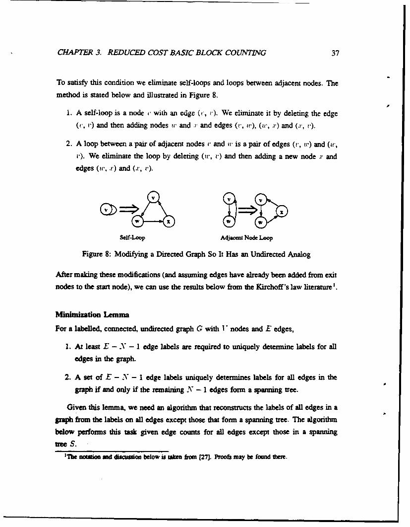
CHAPTER 3. REDUCED COST BASIC BLOCK COUNTING 37
To satisfy this condition we eliminate self-loops and loops between adjacent nodes. The
method is stated below and illustrated in Figure 8.
1. A self-loop is a node c with an edge (c, 0). We eliminate it by deleting the edge
(r, r) and then adding nodes it and .x and edges (", i'), (w, .x) and (x, r).
2. A loop between a pair of adjacent nodes u and ti is a pair of edges (c, u') and (w,
t). We eliminate the loop by deleting (w, t-) and then adding a new node .x and
edges (ic, r) and (x, v).
SCIf-Loop Adjacent Node Loop
Figure 8: Modifying a Directed Graph So It Has an Undirected Analog
After making these modifications (and assuming edges have already been added from exit
nodes to the start node), we can use the results below from the Kirchoff's law literature'.
Minimization Lemma
For a labelled, connected, undirected graph G with V nodes and E edges,
1. At least E - X - 1 edge labels are required to uniquely determine labels for all
edges in the graph.
2. A set of E - N - 1 edge labels uniquely determines labels for all edges in the
graph if and only if the remaining N - 1 edges form a spanning tree.
Given this lemma, we need an algorithm that reconstructs the labels of all edges in agraph from the labels on all edges except those that form a spanning tree. The algorithm
below performs this task given edge counts for all edges except those in a spanning
tree S.
'Mm ntation mad diWcuaon below is taken frmn [27]. Prooft may be found there.
CHAPTER 3. REDUCED COST BASIC BLOCK COUNTING 38
Labelling Algorithm
1. Set the labels of all edges in S to 0.
2. For each edge ( that is not in S, there is a unique cycle in G (called a fundamentalcycle) made up of ( and edges from S.
Traverse the cycle clockwise, edge by edge. If an edge is in S and the direc-tion of traversal matches the direction of the edge, add the label of ( to the labelof the edge, otherwise subtract ('s label.
An example should clarify the statement of the algorithm. Consider again the labelled
flow graph in the figure and take the same maximum cost spanning tree as before: {(/), c),
(c, t), (d, (), (c, .f), (.f, a)). To execute step two of the algorithm for the non-spanning
tree edge (a, b), we traverse its fundamental cycle adding its label (2) as we go:
Traverse (b, c) and add 2 to its label.Traverse (c, f) and add 2 to its label.Traverse (c, f) and add 2 to its label.Traverse (.f, a) and add -2 to its label.
Repeating this process for the other non-spanning tree edges will produce correct labels
on all edges.
3.1.2 Counter Costs
The Minimization Lemma of the previous section tells us that we must place counters on
all the edges of a graph except those that form a spanning tree. If we label each edge in
the control flow graph with the cost to place a counter on it, and then eliminate the edges
that form a maximum cost spanning tree, the remaining edges will offer the minimum
cost measuring scheme with respect to the current edge cost labelling. For the sake of
brevity, in the remainder of the chapter we will refer to these counters as minimum cost,
omitting, but always meaning, with respect to the current edge cost labelling.In this section, we examine the cost of executing an edge counter. The cost of a
counter depends on the particular instructions we use to implement it. Our discussionbelow focuses on implementing counters for the MIPS architecture, but a similar analysis
would apply to other machines. We identify four different classes of counter:
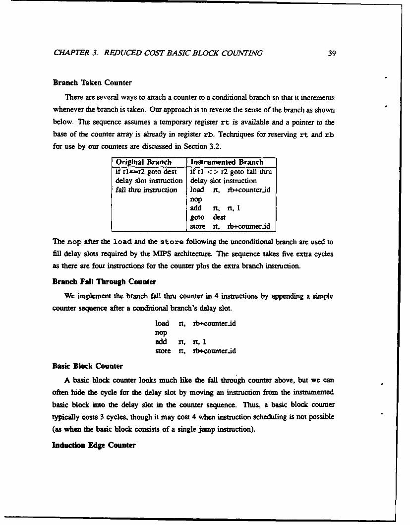
CHAPTER 3. REDUCED COST BASIC BLOCK COUNTING 39
Branch Taken Counter
There are several ways to attach a counter to a conditional branch so that it incrementswhenever the branch is taken. Our approach is to reverse the sense of the branch as shown
below. The sequence assumes a temporary register rt is available and a pointer to the
base of the counter array is already in register rb. Techniques for reserving rt and rb
for use by our counters are discussed in Section 3.2.
Original Branch Instrumented Branchif rl---r2 goto dest if rl < > r2 goto fall thrudelay slot instruction delay slot instructionfall thru instruction load it, rb+counter..id
nopadd rt, rt, 1goto deststore rt, rb+counter.id
The nop after the load and the store following the unconditional branch are used to
fill delay slots required by the MIPS architecture. The sequence takes five extra cycles
as there are four instructions for the counter plus the extra branch instruction.
Branch Fall Through Counter
We implement the branch fall thru counter in 4 instructions by appending a simple
counter sequence after a conditional branch's delay slot.
load nt, rb+counter.idnopadd nt, rt,lstore rt, rb+counter.id
Basic Block Counter
A basic block counter looks much like the fall through counter above, but we can
often hide the cycle for the delay slot by moving an instruction from the instrumented
basic block into the delay slot in the counter sequence. Thus, a basic block counter
typically costs 3 cycles, though it may cost 4 when instruction scheduling is not possible
(as when the basic block consists of a single jump instruction).
Induction Edge Counter

CHA4PTER 3. REDUCED COST BASIC BLOCK COUKTING 40
Basic Block Counter 3-4Branch Taken 5Branch Fall Thru 4Induction Edge Counter 8
Table 7: Counter Cost Per Execution in CPU Cycles
Loop induction variables act as counters that record how many times we go around
a loop. When we detect an induction variable, we can avoid using a standard counter
and instead record the value of the induction variable on loop entry and exit (suitably
normalized by the loop increment). Assuming the loop iterates several times each time it
is entered, this will result in substantial savings over inserting a counter in the loop body.
The induction edge counter is implemented by adding the value of the loop induction
variable to the counter on loop entrance and then subtracting it from the counter on loop
exit. The cost of the counter is around 8 cycles per loop entrance as it involves two 4
cycle counter updates.
The counter costs are summarized in Table 7. Note the costs are MIPS architecture-
dependent, and ignore fancy instruction scheduling that might result in minor cost re-
ductions. For example, we could potentially hide the load delay slot in the taken branch
counter by copying the first instruction of the destination basic block to this slot and then
changing the taken destination to be the second instruction of that block. Such optimiza-
tions were ignored for the sake of simplicity as they would not substantially alter our
results.
Finally, we observe that since 3 cycle node counters are substantially cheaper than
4 and 5 cycle edge counters, they are often preferable. However, a node count may
not correspond directly to any edge label in the control flow graph. We can repair this
problem by transforming the control flow graph as follows: For any node r with multiple
parents and children, add a new node v'. Then, move the outgoing edges of r so they
instead emanate from t'. Finally add an edge (c'). An example is given in Figure 9
The label on (r',r') will correspond to the node counter, and the other edge labels will be
unchanged.
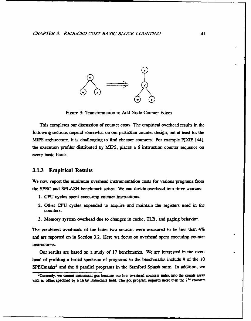
CHAPTER 3. REDUCED COST BASIC BLOCK COLUNTING 41
V
W X
W X
Figure 9: Transformation to Add Node Counter Edges
This completes our discussion of counter costs. The empirical overhead results in the
following sections depend somewhat on our particular counter design, but at least for the
MIPS architecture, it is challenging to find cheaper counters. For example PIX[E [44],
the execution profiler distributed by MIPS, places a 6 instruction counter sequence on
every basic block.
3.1.3 Empirical Results
We now report the minimum overhead instrumentation costs for various programs from
the SPEC and SPLASH benchmark suites. We can divide overhead into three sources:
1. CPU cycles spent executing counter instructions.
2. Other CPU cycles expended to acquire and maintain the registers used in thecounters.
3. Memory system overhead due to changes in cache, TLB, and paging behavior.
The combined overheads of the latter two sources were measured to be less than 4%
and are reported on in Section 3.2. Here we focus on overhead spent executing counter
instructions.
Our results are based on a study of 17 benchmarks. We are interested in the over-
head of profiling a broad spectrum of programs so the benchmarks include 9 of the 10
SPECmarks 2 and the 6 parallel programs in the Stanford Splash suite. In addition, we2Currently, we cannot insuument gcc because our low overhead counters index into the counts array
with un offset specified by a 16 bit immediate field. The gcc program requires more than the 23" counters
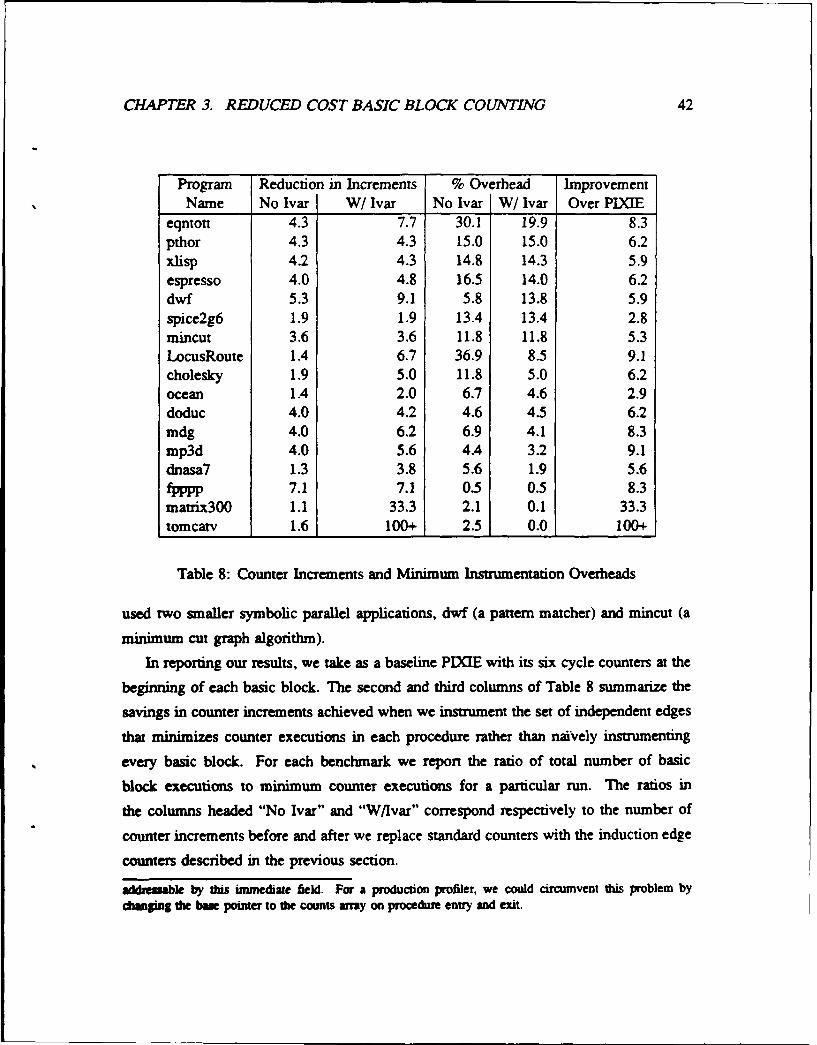
CHAPTER 3. REDUCED COST BASIC BLOCK COUNIWNG 42
Program Reduction in Increments % Overhead ImprovementName No Ivar W/ Ivar No Ivar W/Ivar Over PIXIE
eqntort 4.3 7.7 30.1 19.9 8.3pthor 4.3 4.3 15.0 15.0 6.2xlisp 4.2 4.3 14.8 14.3 5.9espresso 4.0 4.8 16.5 14.0 6.2dwf 5.3 9.1 5.8 13.8 5.9spice2g6 1.9 1.9 13.4 13.4 2.8mincut 3.6 3.6 11.8 11.8 5.3LocusRoute 1.4 6.7 36.9 8.5 9.1cholesky 1.9 5.0 11.8 5.0 6.2ocean 1.4 2.0 6.7 4.6 2.9doduc 4.0 4.2 4.6 4.5 6.2mdg 4.0 6.2 6.9 4.1 8.3mp3d 4.0 5.6 4.4 3.2 9.1dnasa7 1.3 3.8 5.6 1.9 5.6fpppp 7.1 7.1 0.5 0.5 8.3
matrix300 1.1 33.3 2.1 0.1 33.3tomcarv 1.6 100+ 2.5 0.0 100+
Table 8: Counter Increments and Minimum Instrumentation Overheads
used two smaller symbolic parallel applications, dwf (a pattern matcher) and mincut (a
minimum cut graph algorithm).
In reporting our results, we take as a baseline PIXIE with its six cycle counters at the
beginning of each basic block. The second and third columns of Table 8 summarize the
savings in counter increments achieved when we instrument the set of independent edges
that minimizes counter executions in each procedure rather than naively instrumenting
every basic block. For each benchmark we report the ratio of total number of basic
block executions to minimum counter executions for a particular run. The ratios in
the columns headed "No Ivar" and "W/Ivar" correspond respectively to the number of
counter increments before and after we replace standard counters with the induction edge
counters described in the previous section.
addreuable by this immediate field. For a production profiler, we could circumvent this problem bydcangmg the base pointer to the counts array on prooedum entry and eiit.

CHAER 3. REDUCED COST BASIC BLOCK COUNTING 43
Our technique for recognizing induction variables is to rely on the MIPS compiler
(at 02 optimization level). Our analysis routines examine the executable file generated by
the compiler. For each loop in the executable, if there is a register which is incremented
by the same constant on every path through the loop, then we use that register as our
induction variable counter. The MIPS compiler does the real work of identifying the
induction variable and placing it in a register.
Examining the table, we find improvement factors of 1.1 to 7.1 before we exploit in-
duction variables and 1.9 to 100+ afterwards. While the reduction in counter increments
is interesting because it is a property of the program's control flow graph (and hence
somewhat architecture-independent), it is perhaps more relevant to examine the percent-
age overhead introduced by the counter instructions. The final three columns in Table 8
report overhead in terms of CPU cycles only, ignoring all memory system (cache, TLB,
paging) effects. Counting only CPU cycles tends to make the overhead numbers slightly
pessimistic, as our instrumentation adds very little memory overhead (see Section 3.2)
while real programs do lose some performance in the memory hierarchy. Examining the
table, we see overhead varies from about 1 to 37% when we ignore induction variables
and 0 to 20% when we save counter increments by exploiting the induction variables.
The median overhead when using induction variables is just 5%. As we would expect,
overheads are lower for scientific code, where basic blocks are long, and higher for
symbolic programs.
The final column in Table 8 gives the ratio of PIXIE's counter overhead to the
overhead of our minimum cost instrumentation. We see improvements of about 3 to 10,
excepting two outliers (matrix300 and tomcarv) where recognizing induction variables
virtually eliminates overhead. In Graph 1, we break the improvement down into four
sources:
* Savings from independent paths.
e Savings from replacing 6 cycle counters with 3-4-5 cycle counters.
* Savings from recognizing induction variables.
* Savings from choosing the best (minimum) cost set of independent paths.
CHAPTER 3. REDUCED COST BASIC BLOCK COUNTING 44
The programs have been sorted by minimum instrumentation overhead, and there are 5
points associated with each benchmark. We have connected the points to make trends
more visible (though the lines have no inherent meaning). The top solid line is the PIXIE
overhead and the dotted line below it represents the overhead when we place 6 cycle
counters on a random set of independent control paths in each procedure. More precisely,
we use the algorithm in Figure 10 to compute the cost of instrumenting an arbitrary
independent set of control flow paths. Comparing the independent path overhead to the
overhead of instrumenting every basic block, we find the savings is typically a factor of
two.
The dashed line represents the cost of instrumenting a random set of independent paths
with our 3-4-5 cycle counters rather than PIXIE's 6 cycle counters. The improvement
over the expensive counters ranges from about 10% to 100%. It is not as dramatic as the
savings when moving from a counter on every basic block to counters on independent
control paths only.
The next line represents average overhead when we use 3-4-5 counters and. wherever
possible, induction edge counters. The cost of choosing an "average" set of edges is
found using the algorithm of Figure 10, with the slight modification that we always favor
(by assigning high weights) measuring edges corresponding to induction variables. The
amount of savings ascribable to using induction edge counters is program sensitive: we
see a factor of 3 improvement in certain loop oriented code like the NASA benchmark
(dnasa7), LocusRoute, tomcatv, and matrix multiply, but overheads for some of the other
program's are unchanged. It is worth noting that the overheads represented in this solid
line correspond to the overheads that would be incurred when using the instrumentation
algorithm described in [54] which recognizes induction variables and chooses an inde-
pendent set of edges. The final bold line at the bottom of the graph is the minimum
overhead achievable with respect to our counters (as defined at the beginning of Sec-
tion 3.1.1). Note the "average independent edge" case is still a factor of two off from
this lower bound. The overheads on the lower bound line are 1.5 to 10+ times less than
the "optimal" overheads reported in [4] because we use lower cost 345 cycle counters
and exploit induction variables.

CAPT 3. REDUCED COST BASIC BLOCK COUNTING 45
210 Graph 1: Overhead From Pixie to Optimal
10 oe- 9 Pixie Overhead (6 Cycle Counter)
...... * Average: Independent Paths, 6 Cycle Counter+- - -- Average: Independent Paths, 345 Counters
-- c Average: 345 Counters+Induction Variablesu--n Minimum 345 Overhead
150
120,
go-\9
60 i . :It•
30 e* o
4.-
eqn xli spi dwl cho dod mp3 tpp tam
pth esp min Loc oce mdg dna matBenchmark Name

CHAPTER 3. REDUCED COST BASIC BLOCK COLUNTING 46
FOR I = 1 to 7Set COST[I] to 0FOR each procedure in the program
Assign random labels to the edges in theprocedure's control flow graph
Eliminate the minimum cost spanning tree.Add to COST[I] the overhead introduced byinstrumenting the remaining non-spanning.
Output the median value in the COST array.
Figure 10: Finding the "Average" Cost of Instrumenting Independent Edges
In summary, we find twofold improvement by replacing basic block counters with
counters on independent control paths, another 50% gain by using 3-4-5 cycle counters
instead of 6 cycle counters, an improvement by a factor of 1 to 3 by recognizing inductionvariables, and a final factor of 2 by utilizing profile information to select the cheapest
set of control paths to instrument. After taking advantage of all these improvements, we
still incur overhead of 1-20% to collect a profile. Since this overhead is minimal with
respect to our counter costs, there is little hope for achieving extremely low overheads
that might justify leaving profiling enabled in production codes. The numbers offered in
this section do however provide lower bounds to aim for when developing heuristics to
select inexpensive sets of edges to use in profiling.
3.1.4 Heuristics
Given the results of the last section, the natural question to ask is, "How close to this lower
bound can we get by heuristically selecting a set of independent edges to instrument?"We begin with a simple example that shows why we cannot consistently achieve the lower
bounds using a heuristic. The graph in Figure 11 is an abstraction of the control flow
graph used in the examples of Section 3.1.1. The edge labelled Loop Return corresponds
to an induction variable whose value can be captured with very little overhead. To
construct a full execution profile, we should place a counter on the low cost induction
edge and on exactly one of the edges labelled A and B. However, a priori we have no

CHAPTER 3. REDUCED COST BASIC BLOCK COUNTING 47
J LoopA Return
Loop Exit
Figure 11: A Graph That Defies Heuristics
way of knowing the relative number of times the two edges will execute. Without this
information, we cannot minimize overhead.
Despite this example, it is still interesting to explore how well simple heuristics do
on real programs. One possible source of heuristics is the algorithms that optimizing
compilers use to compute estimated profiles. The following typical algorithm is taken
from [63]:
A basic block's count is initially one and is multiplied by ten for each loopthat contains it.
While estimated profiles derived using this algorithm work reasonably well in helping
compilers to guess which basic blocks are executed most frequently, they are not really
appropriate to our problem. We need to place counters on all the edges in the control
flow graph except those that form a spanning tree. Knowing that the basic blocks in
innermost loops are likely to execute often will not help us, as we still need to place
counters in these loops. We must decide which way conditional branches will go, not
whether a loop iterates many times.
Rather than use an estimated profile, our heuristic is based on observations about
which edges we must actually measure in order to construct a full execution profile.
Consider first a loop free procedure like the one shown in the left half of Figure 12. An
obvious property of the graph is that a node always executes at least as many times as
any of its descendants; hence, it seems best to place counters on nodes as far from the
root as possible. The following algorithm implements this heuristic:

CHAPTER 3. REDUCED COST BASIC BLOCK COUMNT1VG 48
5 6
5 6 6
2 3 4
2.% . -. 3 .- *4
1 _ 1000
Figure 12: Applying the Heuristic to a Loop-Free Graph
1. Mark all edges as unmeasured.
2. Perform a depth first search to assign post-order numbers to the nodes.
3. Assign each edge the labeJ of its source node, except for pseudo-edges from leavesto the root node which are labelled with a very large number.
4. Eliminate the maximum cost spanning tree and measure the remaining edges.
The right half of Figure 12 shows the results of applying the heuristic; dashed lines
represent edges that will be measured. The heuristic chooses all of the edges coming
into node 1, and then it makes an essentially arbitrary choice to measure one of the two
incoming edges of node 3.
The heuristic is particularly effective when applied to C programs with boolean ex-
pressions containing multiple clauses where the programmer has optimized the order of
the clauses to minimize the number of conditions that will be evaluated. For example,
in the fragment below, the careful programmer will uty to make clause A the condition
that is most often satisfied:
while (A ll B II C) { loop body)
Our heuristic will lead us to instrunent the edges associated with B and C before A,
which mirrors the programmer's frequency based ordering.

CHAPTER 3. REDUCED COST BASIC BLOCK COUNTING 49
In practice, simple heuristics that deal only with acyclic control flow graphs are
inadequate because programs contain loops. When we can recognize an induction variable
in a loop, we will have the problem described at the beginning of this section (see
Figure 11). That is, for conditional branches in the loop body, we must guess which side
to instrument (though we can use the loop-free heuristic above to guide our choices). Forloops where we cannot recognize an induction variable and associate it with a control
flow graph edge, we use the simple heuristic "Don't instrument a loop return edge." The
rationale behind this heuristic can be understood by examining Figure 13. We assume
Edge Sets
{A,B,C}LOOP IA,B,D}
A Return {A,CD}
D c BCD
Loop Exit
Figure 13: The Cost of Measuring A Loop
the loop return edge is usually taken which implies c > d and c = o + b. As shown
on the right side of the figure, there are four possible sets of edges we can instrument.
Plugging in the c > d and c -r, + 1) relations, it is easy to verify the best choice is the
set {a, b, (d).
Taken together, our observations suggest the following heuristic for choosing edges
to instrument in a control flow graph with N nodes:
1. Perform a depth first search and assign post-order numbers to nodes.
2. Label each edge with the post-order number of its source node. (These numbersrange from 1 to N.)
3. Assign edges corresponding to induction variables the label 0 (highest priority forinstrumentation).
4. Add N to the label of loop return edges that do not correspond to induction variables(lowest priority)
CHAPTER 3. REDUCED COST BASIC BLOCK COUNTING 50
5. Assign pseudo-edges from the leaves to the root priority .Y + 1.
6. Eliminate the maximum cost spanning tree (which contains the lowest priorityedges) and measure the remaining high priority edges.
In developing this heuristic, we have assumed all counter costs are equal, effectively
ignoring the 3-4-5 cycle counters discussed in Section 3.1.2. Initially, we extend this
assumption to evaluate the validity of our reasoning. Graph 2 reports the percentage
overhead of our heuristically placed instrumentation in terms of CPU cycles assuming all
counters require 4 cycles. The top and bottom lines give average and minimum overheads
for each benchmark. As in the previous section, the average overhead is derived by
performing the "instrument a random set of independent control edges" experiment 7
times and taking the median total overhead (see Figure 10). Here, the independent sets
of edges always include the induction variable counters. We see the heuristic consistently
performs above average. In the cases where its performance is still far from the lower
bound, (Ithor, xlisp, espresso, dwf), we identified where the heuristic was failing by
sorting procedures by the difference between the heuristic and optimal instrumentation
overheads. Careful examination of the "bad" procedures showed that for all programs
except xlisp, the problem was analogous to choosing the wrong side of the branch in the
graph of Figure 11. For xlisp, the problem was that there are several loops where the
return edge is not taken, so our heuristic that excludes loop return edges (as justified in
Figure 13) does not apply. There is no obvious remedy for these shortcomings.
We close this section by applying our heuristic using actual 3-4-5 cycle counters.
Initially, the heuristic yielded worse than average overhead because it ignored the fact
that branch taken counters are more expensive. We modified the heuristic slightly to favor
fall-thru edges over taken edges and achieved the results shown in Graph 3. We are not
doing quite as well as in the artificial 4 cycle counter case, but we are still consistently
above average. The interaction between the variable counter cost and branch frequency
makes it more difficult to guess the best set of edges to instrument.

CHAPER 3. REDUCED COST BASIC BLOCK COUNIE•1G 51
0 -Graph 2: Heuristic Effectiveness (444)
35 *-- Average Cost+ Heuristic Cost
o - o Minium Cost
30
10
5-
4
01
4o
44
pth spi 62p Loc 009 cho rap3 fpp tam*qn Al rain dwf clod mdg dna mat
Benchmark Name

CHAPTER 3. REDUCED COST BASIC BLOCK COUNTIVG 52
48 Graph 3: Heuristic Effectiveness (345)48
42 --. Average Cost+ + Huristic Costoc- Minimum Cost
36
30,
24 ,
12
6
01.qn xli spi dwf cho dod mp3 tpp tom
pth esp min Loc Dce mdg dna mat
Benchmark Name

CHAEPTER 3. REDUCED COST BASIC BLOCK COUNTING 53
3.2 Compensating for Instrumentation Overheads
In the previous sections, we have considered only the CPU time required to execute
the instrumentation instructions that implement basic block counters. As noted early in
Section 3.1.3, when we add counters to a program, there are three sources of overhead:
1. CPU cycles spent executing counter instructions.
2. Other CPU cycles expended to acquire and maintain the registers used in thecounters.
3. Memory system overhead due to changes in cache, TLB, and paging behavior.
In this section, we consider all three overheads.
We observed earlier (Section 3.1.2) that our counters require two registers: one to
hold the counter value and one to hold a pointer to the counter in memory. We acquire
these registers by selecting the two statically least used registers in the executable file,
and patching the executable to eliminate uses of these registers (by preceding each use
by a load from memory and following each modification by a store). Table 9 shows
that the overhead of the instructions required to scavenge these two registers is less than
2% except for tomcarv where the overhead is 2.4%. This data implies that the MIPS
compiler rarely needs all 32 registers. If the naive scavenging technique were too costly,
we could try to move the instrumentation step into the compiler so that register allocation
for the instrumentation would be done in conjunction with regular code generation. The
drawback of this method is that it would become more difficult to quantify the effect of
the instrumentation on program behavior as it is extremely difficult to isolate the effects
of the instrumentation instructions on the register allocator.
With register acquisition overhead generally less than 2%, the only source of overhead
left to worry about is memory system effects. Our approach to quantifying memory
system effects is:
1. Measure the execution time of the uninstrumented program (To,,.
2. Measure the execution time of the instrumented program (T,,81).
3. Use the profile generated by the instrumented program and full knowledge of whereinstrumentation instructions were inserted to compute the total CPU cycles spentin instrumentation ( .
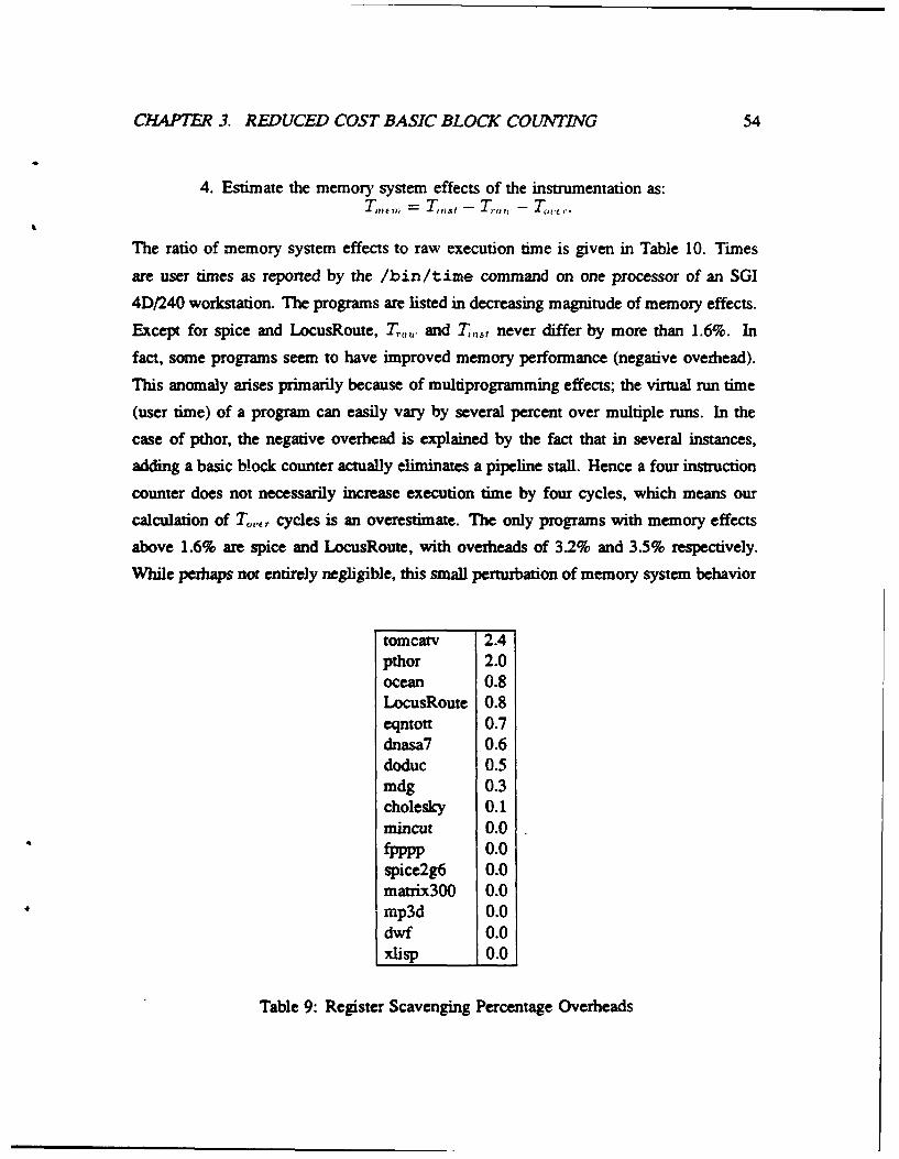
CHAPTER 3. REDUCED COST BASIC BLOCK COUNTI7NG 54
4. Estimate the memory system effects of the instrumentation as:T,,,,, : = T,,,3, - T,,,,,- Tu ,.
The ratio of memory system effects to raw execution time is given in Table 10. Times
are user times as reported by the /bin/time command on one processor of an SGI
4D/240 workstation. The programs are listed in decreasing magnitude of memory effects.
Except for spice and LocusRoute, Th,,,. and T2,,,, never differ by more than 1.6%. In
fact, some programs seem to have improved memory performance (negative overhead).
This anomaly arises primarily because of multiprogramming effects; the virtual run time
(user time) of a program can easily vary by several percent over multiple runs. In the
case of pthor, the negative overhead is explained by the fact that in several instances,
adding a basic block counter actually eliminates a pipeline stall. Hence a four instruction
counter does not necessarily increase execution time by four cycles, which means our
calculation of To,,. cycles is an overestimate. The only programs with memory effects
above 1.6% are spice and LocusRoute, with overheads of 3.2% and 3.5% respectively.
While perhaps not entirely negligible, this small perturbation of memory system behavior
tomcarv 2.4pthor 2.0ocean 0.8LocusRoute 0.8eqntott 0.7dnasa7 0.6doduc 0.5mdg 0.3cholesky 0.1mincut 0.0fpppp 0.0spice2g6 0.0matrix300 0.0mp3d 10.0dwf 0.0xlisp 0.01
Table 9: Register Scavenging Percentage Overheads
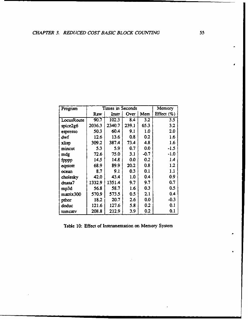
CHAPTER 3. REDUCED COST BASIC BLOCK COUNTING 55
Program Times in Seconds MemoryRaw lnstr Over Mem Effect (%)
LocusRoute 90.7 102.3 8.4 3.2 3.5spice2g6 2036.3 2340.7 239.1 65.3 3.2espresso 50.3 60.4 9.1 1.0 2.0dwf 12.6 13.6 0.8 0.2 1.6xlisp 309.2 387.4 73.4 4.8 1.6mincut 5.3 5.9 0.7 0.0 -1.5mdg 72.6 75.0 3.1 -0.7 -1.0fpppp 14.5 14.8 0.0 0.2 1.4
eqntott 68.9 89.9 20.2 0.8 1.2ocean 8.7 9.1 0.3 0.1 1.1cholesky 42.0 43.4 1.0 0.4 0.9dnasa7 1332.9 1351.4 9.7 9.7 0.7mp3d 56.8 58.7 1.6 0.3 0.5matrix300 570.9 573.5 0.5 2.1 0.4pthor 18.2 20.7 2.6 0.0 -0.3doduc 121.6 127.6 5.8 0.2 0.1tomcarv 208.8 212.9 3.9 0.2 0.1
Table 10: Effect of Instrumentation on Memory System
i I I I i

CHAPTER 3. REDUCED COST BASIC BLOCK COUNTING 56
still seems acceptable.
In particular, the change in memory system behavior introduced by the full counter
instrumentation seems small enough to justify the assumption that T, ...... :, 0 which
means:
=rl Tinst -7*:a*tr - T717fi -, T Y.,st - 7,,.,,?-
Thus, we can recover the raw execution time of an instrumented code by measuring the
actual execution time of the instrumented code (T,,,,,) and using the basic block count
profile and a knowledge of where we inserted instrumentation to compute To,,.,..
3.3 Conclusions on Lightweight Profiling
Above we addressed the problem of minimizing counter overhead when instrumenting a
program to collect basic block count and branch frequency information. We offered an
algorithm for selecting the minimum cost set of edges to instrument given the cost of
measuring every edge in a control flow graph. This algorithm allows us to establish lower
bounds on instrumentation overhead. In practice when minimizing overhead is really
critical, as when instrumenting parallel programs where the effect of the instrumentation
is difficult to quantify, the algorithm allows us to use an execution profile from an initial
run to minimize instrumentation overhead in later runs.
After examining 9 programs from the SPECmarks and 8 parallel programs, we con-
clude that for general programs executing on a typical RISC architecture with counters
that cost around 4 cycles, we must accept instrumentation overheads of 1-20%. If we
limit ourselves to the floating point intensive numerical applications among these 17
applications, the overhead is more like 1-5%.
Our attempt to approach this lower bound by developing heuristics that select cheap
edges to instrumem was moderately successful. By using induction variable counters
where possible, discriminating against loop back edges, and favoring deeper nodes in
the control flow graph over shallower ones, we consistently selected relatively cheap
sets of edges to instrument and came within a factor of two of the lower bound. In
this dissertation, we normally have an execution profile available to guide us in choosing
which edges to instrument, so developing good heuristics is not a high priority. However,
CHAPTER 3. REDUCED COST BASIC BLOCK COUNTING 57
we remain skeptical that one can ever guess which control flow edges will be least
frequently traversed when a program is run.
The profile provides an additional method of controlling basic block counting over-
head. Basic block counting instrumentation is only necessary where the ideal compute
time profile is of interest. In particular, an important way to minimize intrusiveness is
to avoid adding basic block counters to synchronization constructs like spin loops. In
a simple programming model, all time spent in a synchronization construct is viewed
as synchronization overhead (though it may include time spent waiting on the memory
hierarchy); hence, there is no reason to collect basic block count information on the
synchronization construct.
Similarly, some procedures like simple math library functions may be deemed to have
low or acceptable memory overhead, and basic block counting instrumentation can be
omitted for them. For example, the absolute value routine rarely has interesting memory
behavior3 , and it is relatively expensive to count its basic blocks because they are short.
One can easily use an initial execution profile to identify procedures that do not perform
a significant number of global memory operations and are costly to instrument, and then
omit basic block count profiling for such procedures in subsequent runs.
3.4 Counter Perturbation in Parallel Programs
Previous sections have shown that the intrusiveness of full basic block counting is small in
sequential programs. Perhaps more importantly, Section 3.2 demonstrated that the effects
of the basic block counting instrumentation can be isolated and subtracted out. For parallel
programs, compensating for the intrusion of instrumentation is more difficult. In this
section, we outline the nature of the problem and review the literature on compensating
for perturbation in parallel programs. Then, we give some actual results on the overhead
introduced by adding basic block counting instrumentation to ten applications.
The obvious drawback of adding software instrumentation to parallel programs is that
the instrumentation instructions can change the relative timing of the parallel tasks and
31t is diffcult to guanntee the lack of instruction cache effects, so one can seldom be certain that aprocedure will execute without memory system ovefthd.

CHAPTER 3. REDUCED COST BASIC BLOCK COUNTING 58
Task Run Wall Clock Time Synchronization Overhead InstrumentationType Raw Code Instrumented Raw Code Instrumented Overhead(1,1) Seq 2 3 - - 50%
Par 1 2 0 1 100%(2,1) Seq 3 4 - - 33%
Par 2 2 1 0 0%
Table 11: Possible Effects of Instrumentation
distort synchronization overhead. We begin with two examples that illustrate how simple
instrumentation can increase or decrease synchronization overhead. Consider a program
that spawns two tasks TI and T2, exiting when both tasks complete. In this context,
we use the term synchronization overhead to refer to the time when a processor is idle
because it has completed its task and is waiting for the other processor to finish the other
task. Suppose TI and T2 both take 1 second to execute. Assume further that when
we add basic block counting instrumentation to T1, we introduce negligible overhead
(e.g. we can recognize and exploit an induction variable to implement a cheap counter).
However, the basic block counting overhead is significant for 12 which is slowed 100%
so it takes 2 seconds to execute with instrumentation. The first entry in Table 11 gives
the wall clock times, synchronization overheads, and instrumentation overheads for se-
quential and parallel runs of the program. Note how the instrumentation changes the
relative execution times of tasks TI and T2, introducing I second of synchronization
overhead in the instrumented parallel code which did not exist in the uninstrumented run.
This synchronization overhead causes the effective instrumentation overhead (defined as
(Instrumented Time - Raw Thne)/(Raw Time)) to double when moving from sequential
to parallel mode.
It is equally possible, however, that instrumentation will decrease rather than increase
synchronization overhead in the instrumented code. Suppose that task TI has a raw
execution time of 2 seconds rather than 1 second and retain the assumption that we can
instrument TI with negligible overhead. Then, as shown in the second entry of Table 11,
the instrumentation overhead has no effect on wall clock time!
In our simple two task example, we can analyze and compensate for the effects of

CHAPTER 3. REDUCED COST BASIC BLOCK COUNTING 59
instrumentation overhead on synchronization overhead. In fact, several research efforts
are under way to model and compensate for the perturbation that instrumentation intro-
duces into parallel programs. The most extensive work has been carried out by Malony
at Illinois [38, 37]. Malony distinguishes two kinds of perturbation models: total execu-
tion time models and event-based models. Total execution time models use the method
described in Section 3.2 to recover raw execution time from instrumented execution time
by subtracting out the time spent in instrumentation. The technique generalizes to the
parallel domain by assuming processes in the program do not interact and estimating raw
execution time of the parallel program as:
min (Instrumented Time in P - Overhead in P)
Processes P
Note, this model would correctly recover the total execution times of the very simple
programs in Table 11.
In general, however, it is unrealistic to expect that processes in a parallel program will
not interact. Researchers have tried to handle the more general case by observing that
synchronization events impose a partial order on the execution of interacting processes.
For example, all processes must reach a barrier before any process proceeds beyond it. By
recording enough information about synchronization events in the instrumented program
and modeling the constraints imposed by synchronization, we can attempt to reconstruct
execution times for an uninsumented run of the program. Malony describes such models
as event-based because they explicitly consider synchronization events. More formal
models are explored in [1] where parallel programs are represented as timed Petri-nets
and well understood techniques from control theoretic perturbation analysis are applied
to compensate for instrumentation overhead.
Regrettably, the event-based and Perri-net perturbation analysis techniques are not
directly applicable to basic block counting. Both techniques require time-stamped event
traces of synchronization as well as data on the time spent executing instrumentation
code between synchronization events. However, with basic block counters, we know only
the total overhead associated with a particular counter, not the exact overhead incurred
between a particular pair of synchronization events. For example, if a procedure ends
in a barrier, the perturbation analysis requires individual basic block counting overheads

CHAPTER 3. REDUCED COST BASIC BLOCK COUNTING 60
for each call to the procedure, but we only have a single aggregate overhead for the
procedure. Thus, perturbation compensation techniques that rely on trace data are not
immediately applicable.
A second problem with perturbation analysis is that it cannot account for changes
in control flow that arise, for example, when task-queue based search programs are per-
turbed. Thus, while research in perturbation analysis is active, it is neither immediately
relevant to our problem, nor is it completely robust. One practical alternative to compen-
sating for instrumentation overhead in general parallel programs is to use only lightweight
instrumentation and then to compare the actual wall clock times for raw and instrumented
runs of the parallel program. For most programs, it is reasonable to assume that if the two
times are comparable, then the instrumentation has not dramatically altered the program's
behavior and the performance data recorded should be relevant and useful.
Table 12 provides data on the overheads introduced by basic block counting in ten
parallel programs4 . The overheads are defined in terms of the difference between instru-
mented and uninstrumnented run times, and the column labelled L gives the difference
between the overheads for the parallel and sequential runs. The three negative entries
in the column correspond to programs where effective overhead decreased in the par-
allel run versus the sequential run. For six of the ten programs, the difference in wall
clock time for uninstrumented and instrumented runs of the parallel program is less than
10%. The remaining four programs require more selective instrumentation to reduce ba-
sic block counting overheads. One reasonable technique is to use the simple optimization
suggested in Section 3.3: omit basic block counters in procedures where instrumenta-
tion overhead is high and few memory operations are performed. For example, the
check.intersection routine in radiosity is responsible for half the instrumentation
overhead in the sequential program and performs less than 1% of the memory operations.
If we remove basic block counting instrumentation from check-intersection, then
instrumentation overhead for the parallel program is reduced from 18% to 10%. Similarly,
in water, we can omit instrumentation from fabs and reduce the overhead in the parallel
run from 10% to 7%. Thus, for eight of our ten parallel applications, the instrumentation
4'The nmbes in Table 12 me not directly comparable to results reported in the first part of the chapterbecame differmt compiler revisions and in some cases different mput cues were used in the two studies.
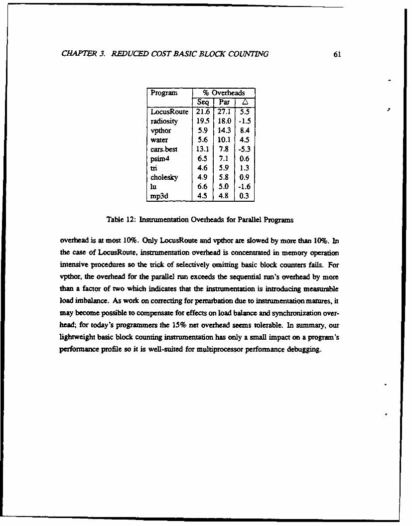
CHAPTER 3. REDUCED COST BASIC BLOCK COUNTING 61
Program % OverheadsSeq Par L
LocusRoute 21.6 27.1 5.5radiosity 19.5 18.0 -1.5vpthor 5.9 14.3 8.4water 5.6 10.1 4.5cars.best 13.1 7.8 -5.3psim4 6.5 7.1 0.6tri 4.6 5.9 1.3cholesky 4.9 5.8 0.9lu 6.6 5.0 -1.6mp3d 4.5 4.8 0.3
Table 12: Instrumentation Overheads for Parallel Programs
overhead is at most 10%. Only LocusRoute and vpthor are slowed by more than 10%. In
the case of LocusRoute, instrumentation overhead is concentrated in memory operation
intensive procedures so the trick of selectively omitting basic block counters fails. For
vpthor, the overhead for the parallel run exceeds the sequential run's overhead by more
than a factor of two which indicates that the instrumentation is introducing measurable
load imbalance. As work on correcting for permrbation due to instrumentation matures, it
may become possible to compensate for effects on load balance and synchronization over-
head; for today's programmers the 15% net overhead seems tolerable. In summary, our
lightweight basic block counting instrumentation has only a small impact on a program's
performance profile so it is well-suited for multiprocessor performance debugging.
Chapter 4
Mtool: A Multiprocessor Performance
Debugger
Broadly stated, the purpose of a performance debugging tool is to focus the user's at-
tention on where a program is spending its time and to give as much insight as possible
into how to reduce the time spent in performance bottlenecks. Our approach to achiev-
ing the latter goal is to break execution time into categories with natural analogs in the
programming model. In Chapter 1, we proposed the following taxonomy:
1. Compute Time: The processor is performing work.
2. Memory Overhead: The processor is stalled waiting for data.
3. Synchronization Overhead: The processor is idle waiting for work.
4. Extra Parallel Work: The processor is performing work not present in the originalsequential code.
In this chapter, we elaborate on this taxonomy, exploring how to measure its various
components and how to report the measurements in a manner that matches the user's
programming model. Specifically, we describe Mtool, an integrated performance debug-
ging system for shared memory multiprocessors. The system uses lightweight software
instrumentation that perturbs the program execution only slightly while gathering enough
data to characterize the program in terms of this execution time taxonomy.
62
CHAPTER 4. MTOOL: A MULTIPROCESSOR PERFORMANCE DEBUGGER 63
4.1 Compute Time and Memory Overhead
The Mprof tool introduced in Chapter 2 provides a way to distinguish compute time
from memory overhead in sequential programs. Our task in this section is to generalize
Mprof's technique of comparing ideal compute time and actual execution time to the
multiprocessor domain. As mentioned in Chapter 3 the reason Mprof isn't immediately
applicable to parallel programs is that it gathers its two profiles in separate runs. Because
of subtle timing dependencies in parallel programs, distinct runs of a program may not
be directly comparable.
To circumvent this problem, we must collect both the actual execution time and the
basic block count profile in a single run. The drawback of moving from a two run imple-
mentation to a single run implementation is that the basic block counting instrumentation
can perturb the parallel program's execution, making it difficult to recover a representa-
tive actual execution time profile. Chapter 3 addressed the problem of reducing the cost
of basic block counting. In particular, we saw in Section 3.2 that for sequential programs
we can recover raw total execution time for a program from instrumented execution time
by subtracting out the time spent executing instrumentation. This compensation algorithm
succeeds because we only need to account for ideal compute time effects; the memory
system behavior of the instrumented code is virtually unchanged.
This empirical result may not hold generally because in some systems the increase in
code size associated with software instrumentation will impact instruction cache perfor-
mance. For the SGI machine where we performed our experiments, this effect was not
pronounced because the machine has an external 64KB instruction cache. Many recent
CPU implementations include small on-chip caches that may, in rare cases, be sensitive
to the moderate increases in code size associated with software instrumentation. Fortu-
nately, for typical parallel programs, the instruction cache behavior of single processor
and multiple processor runs are comparable, so one can use Mprof's two run approach to
isolate instruction cache effects in parallel programs by studying a sequential run. Since
programmers normally optimize a sequential code before parallelizing it, using Mprof
before applying Mtool should be acceptable.
Mprof does not, however, solve the problem of accounting for the impact of basic

CHAPTER 4. MTOOL: A MULTIPROCESSOR PERFORMANCE DEBUGGER 64
block counting instrumentation on synchronization overhead. The most straightforward
solution to this problem would be a three run approach that separated the accumula-
tion of synchronization overhead information from the collection of memory overhead
information:
1. Run the program once with instrumentation that measures synchronization over-head.
2. Run the program again to gather an initial basic block count profile.
3. Use the initial profile to add lightweight instrumentation for memory overheadprofiling.
The problem with the three run approach is that it violates a key tenet of programming
environments: convenience of use.
The preferred alternative to the three run approach is to gather memory overhead
information without substantially distorting synchronization overheads. Then, we can
record synchronization overheads (using techniques that are described in the next sec-
tion) while simultaneously measuring compute time and memory overhead. At the end of
Chapter 3, we offered data that showed the impact of the basic block counting instrumen-
tation on actual wall clock time for parallel programs was small (typically less than 10%).
Further, we saw the net overhead introduced by basic block counting instrumentation did
not differ substantially for sequential and parallel runs of a program. We interpret these
two facts as indirect evidence that synchronization overheads are not radically altered by
the basic block counting instrumentation.
To summarize, we can collect compute time and memory overhead information on a
parallel program without substantially distorting its synchronization behavior. Figure 14
presents the algorithm. The first step is to collect a basic block count profile for use
in controlling overhead in the fully instrumented run. As discussed in Section 2.1, we
obtain the profile by augmenting the executable with counter instrumentation. For a
parallel program, we modify the code so that each process collects basic block counts
in private memory above its stack. When a process exits, it writes these counts to a file
whose name is based on the process identifier.
The next step is to use the profile information to instrument the parallel program with
low overhead basic block counters and timers. If pc-sampling is used to collect actual

CHAPTER 4. MTOOL: A MULTIPROCESSOR PERFORMANCE DEBUGGER 65
1. Instrument with basic block counters and gather a profile.
2. Instrument to collect ideal and actual time profiles:
(a) Enable pc-sampling or insert explicit timer reads as described in Chap-ter 2.
(b) Use the profile information to insert low cost basic block counters asdescribed in Chapter 3.
3. Run the fully instrumented code and correlate the estimated and actual timeprofiles to isolate memory overheads.
Figure 14: Creating a Memory Overhead Profile with Mtool
time information (and overhead control is not a primary concern), we can actually skip
the initial profiling of Step I and implement Step 2b using the heuristics of Section 3.1.4
to guide the insertion of basic block counting instrumentation.
It is interesting to note that Figure 14 closely resembles Figure 2 where we described
the Mprof implementation that uses explicit clock reads to measure actual time. This
resemblance is natural because both the m-object selection process and reduced cost basic
block counting exploit the same principle: an initial basic block count profile allows us
to estimate and control the overhead introduced by instrumentation.
While we can view the algorithm of Figure 14 as a natural extension of Mprof, the
description ignores a critical aspect of parallel programming, processor idle time.
4.2 Synchronization Overhead
For Mtool to fully characterize the performance of a parallel program, it must help the
user to understand synchronization as well as memory bottlenecks. We define synchro-
nization overhead as any time when a processor is idle (or spin-waiting). The nature of
synchronization delays depends strongly on the parallel programming paradigm. Here
we describe Mtool's measurement scheme for two paradigms: C programs augmented
with the ANL macros and Fortran programs whose DO loops are parallelized by the SGI
"Power Fortran" compiler.
The ANL macros [6] provide a portable shared memory abstraction with constructs
for process creation, shared memory allocation, parallel loops, locks, barriers, and other

CHAPTER 4. MTOOL: A MULTIPROCESSOR PERFORMANCE DEBUGGER 66
ANL Macros Fortran (parallelized)
Load Some processes are active while Some processes are active whileImbalance others wait at a global synchro- others wait at the barrier at the
nization point (barrier) or on an end of a parallel loop.empty task queue.
Critical A region or resource is protected In dynamically scheduled loops,Section by a lock so only one processor a lock protects the next available
can access it (e.g., global counter iteration counter.update).
Sequential Sequential startup and shutdown Either the program is executing aTime time when a master process ini- parallel loop or it is running se-
tializes or post-processes data be- quentially and all slaves are idle.fore and after the parallel portionof the program.
Figure 15: Sources of Synchronization Loss
synchronization primitives. ANL macro programs tend to be structured as a single master
process that performs some initialization and then spawns slave processes to cooperate
in solving a problem. Similarly, Power Fortran programs use a master process to spawn
slaves. The master executes sequential portions of the code while iterations of parallelized
DO loops are distributed across all processors. By default, the loop iterations are divided
into equal sized contiguous chunks and assigned to processes. The user may optionally
specify interleaved allocation of iterations or various dynamic self-scheduling methods.
A barrier is used to synchronize at the end of each parallel loop.
Figure 15 provides a framework for understanding synchronization overhead losses in
these programming paradigms. The categories in the figure are neither mutually exclusive,
nor exhaustive. In particular, they ignore complicated event-driven interactions among
tasks where processor 1 waits to be signaled by processor 4 which then signals processor
3, etc. Such complicated interactions have not appeared in the compiler parallelized
Fortran or ANL macro programs we have available to us, but we do describe ways to deal
with them in our discussion of attention focusing in Section 4.4. Here we concentrate
CHAPTER 4. MTOOL: A MULTPROCESSOR PERFORMANCE DEBUGGER 67
on how to measure simple synchronization overheads in the ANL macro and Fortran
programming environments.
4.2.1 ANL Macros
For the ANL macros, Mtool needs to instrument locks and barriers to measure waiting
times and to add explicit timers to record when the first parallel slave is spawned and
when the final slave is retired. With this timing information, the user can detect load
imbalance as time spent waiting at a barrier, critical section overhead as time spent
waiting at the lock that protects the critical section, and starvation during startup and
shutdown via the explicit timing of these phases of the program's execution.
There are two complications that must be handled when instrumenting ANL macro
synchronization. The first is an artifact of the relatively expensive (25 cycle) locks
provided on our SGI machines: programmers often ignore the ANL LOCK macro and
synchronize by spinning until a location's value is set. Mtool must be able to understand
user-defined synchronization loops to give an accurate picture of program performance.
Mtool's approach is to allow the user to specify a synchronization loop in a ".usynchs"
file containing triples of the form (File Name, First line of loop, Last
line of loop). Mtool then treats these loops as spin locks.
The second complication is the overhead incurred when timing fine-grained syn-
chronization. Of course, the extent to which this is a problem depends on the kind of
timers that are used. Below we describe Mtool's approach to measuring synchronization
overhead for any of several levels of timer support. We consider both the case when
synchronization is implemented inline and when synchronization routines are accessed
via procedure calls (e.g. lock () is a library routine).
To avoid perturbing program execution, the method of choice for measuring synchro-
nization overhead in Mtool is pc-sampling. The applicability of pc-sampling depends
on whether the region of code to be timed includes only inline code or contains proce-
dure calls as well. In particular, simple pc-sampling does not capture information about
which call sites are responsible for most of the time spent in a particular synchronization
routine. There may be 40 seconds total spent in lock 0, but which locks are actually

CHAPTER 4. MTOOL: A MULTIPROCESSOR PERFORMANCE DEBUGGER 68
experiencing contention?
The ideal solution is a user level interrupt service which calls a user supplied handler
in the user process at regular intervals'. This handler increments the bucket correspond-
ing to the program counter, except when the currently executing instruction lies in a
synchronization procedure in which case the handler increments the bucket associated
with the instruction that called the synchronization procedure. The address of the caller
can typically be found by tracing the call stack or simply examining the return address
register.
When user level interrupts are not supported or higher resolution timing is desired,
Mtool uses explicit timers. If low overhead (1-2 cycle) clocks are available, Mtool
instruments all locks, barriers, and user synchronization loops. For synchronization en-
capsulated in procedures, Mtool simply places clock reads around synchronization call
sites: the cost of reading the clock is dominated by the cost of executing the call-return
sequence and the instructions that enforce the synchronization (even if the synchronization
request is granted immediately).
In some cases, however, synchronization is inline and extremely fine-grained. The
following fragment is an abstraction of an example of a user synchronization loop we
encountered elsewhere [23]. It shows a busy-wait loop used to guarantee that no element
of the vector X is accessed before its Rf ody bit is set:
while (j++ < N) {while (!Ready[j]) /* busy-wait */
y[j] -= xU) * a[k]U];
In this example, if R ,dy[.j] is true, the busy wait loop executes in 4 cycles on an
SGI system; even two inexpensive clock reads around the loop will certainly perturb the
program. Mtool avoids this pitfall by instrumenting the busy-wait loop so the timer calls
are executed only if R(aod.o[i. is initially false:
'The UNIX setitimer system call provides a user level interrupt service, but the internuptis deliveredusng software signals. This renders the service inappropriate for sampling because signals are sent only onfull context-switches rather than at truly regular intervals independent of the program execution. At leastone multiproessor design, the Paradigm system [10] features explicit hardware support to help implementregular, fine-grained delivery of interrupts to user processes.

CHAPTER 4. MTOOL. A MULTIPROCESSOR PERFORMANCE DEBUGGER 69
while 0++ < N)jif (!ReadyU]) {
StanTime = ReadClockO;repeat
until (Ready[j])TotalTime += ReadClock0-StartTime;
Iy[j] - x[jJ * a[k][j];
On systems that generate code with the MIPS compiler, this optimization is simple to
implement because the compiler automatically transforms a while or for loop into
a repeat-until loop protected by an initial guard condition. Mtool can place its
instrumentation after the guard condition and the overhead of using explicit timers will
be reasonably low.
The final case we consider is measuring synchronization overhead with medium cost
(10-50 cycle) off-processor clocks like those found on current SGI systems. When
synchronization is inline (or when linkage tailoring is used to create a distinct copyof a synchronization procedure for each call site), Mtool will use pc-sampling rather
than intrusive explicit timer calls. Otherwise, Mtool uses the following hybrid selectivr
instrumentation/pc-sampling technique:
1. Measure the aggregate time in each synchronization routine with pc-sampling.
2. Allow the user to selectively place timers around synchronization call sites.
3. For each synchronization procedure, report:
"* Total Explained Tune (time measured at instrumented call sites)
"* Other Time (Aggregate Execution Time - Total Explained Tune)
Step 2 is implemented by maintaining a ".synchs" file analogous to the ".usynchs" file
with a tuple of the form:
(source file, procedure name, line number, synchronization type, timing status)
for each synchronization call site. The user can determine whether or not a call is timed
by toggling the timing status. While effective in practice, we consider this toggling

CHAPTER 4. MTOOL: A MULTIPROCESSOR PERFORMANCE DEBUGGER 70
Clock Type Synch. Type What's Measured Extra OverheadUser Level Inlne Individual Synch Sites NoneSampling Procedural Individual Synch Sites Maintain Synch ID's
Kernel Level Inline Individual Synch Sites NoneSampling Procedural Aggregate Times Only None
Low Overhead Inline Individual Synch Sites Clock Reads
Tuners (1-2 cycles) Procedural Individual Synch Sites Clock Reads
Medium Overhead Inline Not SupportedTimers Procedural Selected Synch Sites/ Clock Reads
(10-50 cycles) I Aggregate Times
Table 13: Timing ANL Macro Synchronization
mechanism an unfortunate necessity as it requires assistance from a potentially naive
user. One of Mtool's goals is to use heuristics to reliably and automatically instrument
code with low intrusiveness and high accuracy. We anticipate that future machines will
provide better timing support so that the need for user intervention can be eliminated.
Mtool's approach to synchronization overhead, measuring the time spent in locks and
barriers, is quite similar to using preprocessors or instrumented libraries/macros which
add clock timer calls to locks and barriers (e.g., [13]). The advantage offexed by Mtool is
that it is "cognizant" of intrusiveness: As summarized in Table 13, regardless of the type
of timing mechanism, Mtool offers a low overhead method of measuring synchronization
overhead.
4.22 Compiler Parallelized Fortran
Mtool's support of parallel Fortran is tailored to the simple loop-level model of paral-
lelism. A parallel loop is executed as follows on the SGI system:
I. The master process gives each slave a pointer to a procedure which encapsulatesthe original loop body. This loop body procedure is invoked with arguments thatspecify which loop iterations are to be performed.
2. While iterations are available, the slaves and master cooperate in executing itera-tions of the parallelized loop by calling the loop body procedure. For example, inthe simple statically scheduled case with P processors and ._ P total iterations,process i calls the loop body procedure to do iterations (I - 1) * Y to N* .
CHAPTER 4. MTOOL: A MULTIPROCESSOR PERFORMANCE DEBUGGER 71
3. When a process completes its iterations it synchronizes at a barrier. The mastercontinues when all processors have reached the barrier.
For each parallel loop, Mtool collects two times:
"* Wall clock time in parallel mode (T,,,,).
"* Aggregate time spent in the procedure that implements the loop body (T,,.,,rk).
T,,,, is the total time the master process is in parallel mode; it can be measured by placing
clock reads immediately before the master enters a parallel loop call and immediately
after the parallel call returns. If P is the total number of processors, then we define loop
overhead as T,,,.- (T .,,.,./P . This overhead is a combination of scheduling overhead
and load imbalance. Since Mtool collects the T,,Qr,. time for each individual process, it
can also provide the user with the minimur,j anr aiaximum total work in each parallel
loop over all processes. This information ýL-n , useful in detecting situations where
static scheduling produces a load imbalance. The case study of Section 5.1 should
clarify the meaning and relevance of these measurements. The main idea is that Mtool's
synchronization model for parallel Fortran matches the programming model: execution
time is broken into sequential and parallel time, with parallel time subdivided into work
and loop overhead.
4.3 Parallel Overhead
The final category in Mtool's bottleneck taxonomy is extra work. On the SGI machine,
parallel control operations ulk- spawning tasks and allocating locks are invoked with
procedure calls. Mtool uses its basic block counting technique to estimate time spent
in such procedures and designates this time as parallel overhead. Mtool also associates
a certain amount of parallel overhead with each synchronization call. For example, as
noted earlier, even when there is no contention for a lock on the SGI machine, it still takes
about 25 cycles to acquire. This necessary extra work is attributed to parallel overhead
rather than to synchronization time.
The user has some flexibility in defining extra work. Mtool determines which pro-
cedures are parallel overhead by reading a file of procedure names, and the user can

CHAPTER 4. MTOOL: A MULTZPROCESSOR PERFORMANCE DEBUGGER 72
customize this file. In addition, if extra work is of particular concern, the user can dis-
play Mtool's results for single and multiple processor runs side by side and compare
them. Differences in the aggregate estimated time for procedures in the single and mul-
tiple processor runs represent extra work (or superlinear speedup). An example from an
actual performance debugging session is reported in Section 5.4.
4.4 Attention Focusing Mechanisms
While collecting data with minimal intrusion is a necessary part of any performance
debugging environment, the immediate utility of an environment depends on how it
organizes, filters, and presents the data to the programmer. In this section, we introduce
Mtool's attention focusing mechanisms and compare and contrast them with features
available in other performance debugging systems.
4.4.1 User Interface
To make our discussion concrete, we first describe Mtool's user interface. Figure 16
presents the summary window Mtool provides when displaying the profile of a sparse
triangular back solver (TRI) written with the ANL macros. The top portion of the
window reports information about when the slave processes are created and destroyed,
both textually as startup/shutdown time and graphically as a time line. The bottom half
of the window gives aggregate information on the bottlenecks in the execution time
taxonomy. The Total, Min, and Max columns correspond respectively to the sum
over all processes, the minimum for any process and the maximum over all processes of
each taxonomy element. System time is just the operating system's notion of the time it
spends doing work on behalf of the processes while parallel overhead is the fixed cost
associated with locks and baniers as described in Section 4.3. The shaded horizontal bar
corresponds to the textual inform -t'ion, with the length of the shaded regions proportional
to the time spent in each of the taxonomy categories. Unexplained time represents
memory or synchronization overhead that has not been explicitly measured by Mtoolprobes-
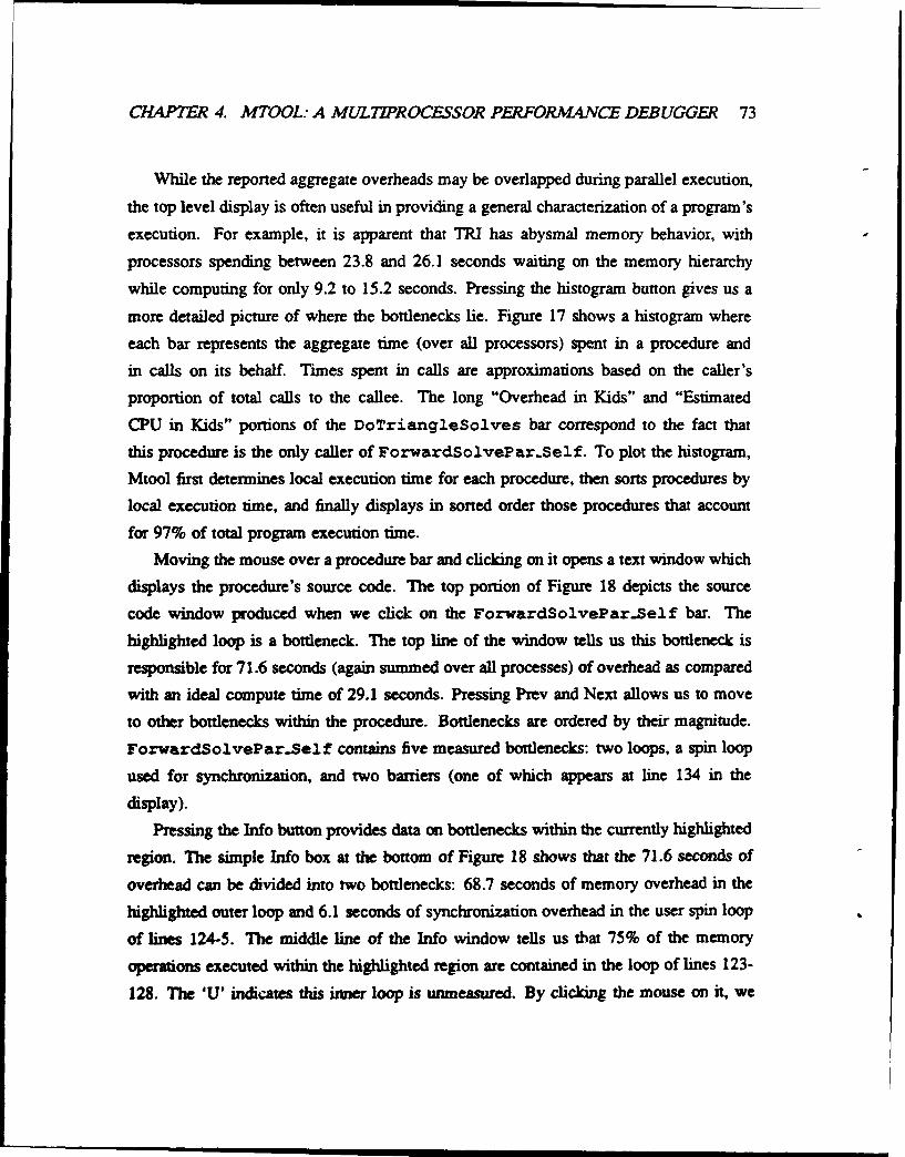
CHAPTER 4. MTOOL: A MULTIPROCESSOR PERFORMANCE DEBUGGER 73
While the reported aggregate overheads may be overlapped during parallel execution,
the top level display is often useful in providing a general characterization of a program's
execution. For example, it is apparent that TRI has abysmal memory behavior, with
processors spending between 23.8 and 26.1 seconds waiting on the memory hierarchy
while computing for only 9.2 to 15.2 seconds. Pressing the histogram button gives us a
more detailed picture of where the bottlenecks lie. Figure 17 shows a histogram where
each bar represents the aggregate time (over all processors) spent in a procedure and
in calls on its behalf. Times spent in calls are approximations based on the caller's
proportion of total calls to the callee. The long "Overhead in Kids" and "Estimated
CPU in Kids" portions of the DoTriangleSolves bar correspond to the fact that
this procedure is the only caller of ForwardSolvePar.Self. To plot the histogram,
Mtool first determines local execution time for each procedure, then sorts procedures by
local execution time, and finally displays in sorted order those procedures that account
for 97% of total program execution time.
Moving the mouse over a procedure bar and clicking on it opens a text window which
displays the procedure's source code. The top portion of Figure 18 depicts the source
code window produced when we click on the ForwardSolveParSelf bar. The
highlighted loop is a bottleneck. The top line of the window tells us this bottleneck is
responsible for 71.6 seconds (again summed over all processes) of overhead as compared
with an ideal compute time of 29.1 seconds. Pressing Prey and Next allows us to move
to other bottlenecks within the procedure. Bottlenecks are ordered by their magnitude.
ForwardSolvePar.Self contains five measured bottlenecks: two loops, a spin loop
used for synchronization, and two barriers (one of which appears at line 134 in the
display).
Pressing the Info button provides data on bottlenecks within the currently highlighted
region. The simple Info box at the bottom of Figure 18 shows that the 71.6 seconds of
overhead can be divided into two bottlenecks: 68.7 seconds of memory overhead in the
highlighted outer loop and 6.1 seconds of synchronization overhead in the user spin loop
of lines 124-5. The middle line of the Info window tells us that 75% of the memory
operations executed within the highlighted region are contained in the loop of lines 123-
128. The 'U' indicates this inner loop is unmeasured. By clicking the mouse on it, we

CHAPTER 4. MTOOL: A MULTIPROCESSOR PERFORMANCE DEBUGGER 74
0 MTOOL: tri (File is rc.tri.4) Ir I ,Time fo-- Master (sec-) Time
0 9 IS 27 3E, 45
Total: 4E.00IStartup: 9.0o haste
Shutdown: 01.00 Samvel
£lave3
Total Min max
.-. Esti.. CPU Time: 43.69 9.23 15.23*M emorg Overhead: 100.02 23.82 26.10 measured 91% mops
m Srech Overhead: 12.92 2.00 4.54Sqz Time: B.4" 0.72 1.20
MPar. Overhead: 0.02 0.00 0.00UnexpI a ined: 6.15 --
I Eyit1 r Histogral, 3
Figure 16: Mtool Summary W•mdow
Fel Histogram (File rc.tri.4)Overhead (irn kids)
1 Svnchm Me.ory.K Est. CPU (in kids)
SEst. CPU
120.,..-.- . . -,oO.o.. . . . .
: -.. .. -. :.'.. . . . .J.,,9 0 ::::::::::::s o .............::::::
,..o -.. -.. -.....-. :.
30
For'mardSolvePar_.$elf Doir ian91eSo 1vescachef lush
Procedure
Figure 17: Mtool Procedure Histogram
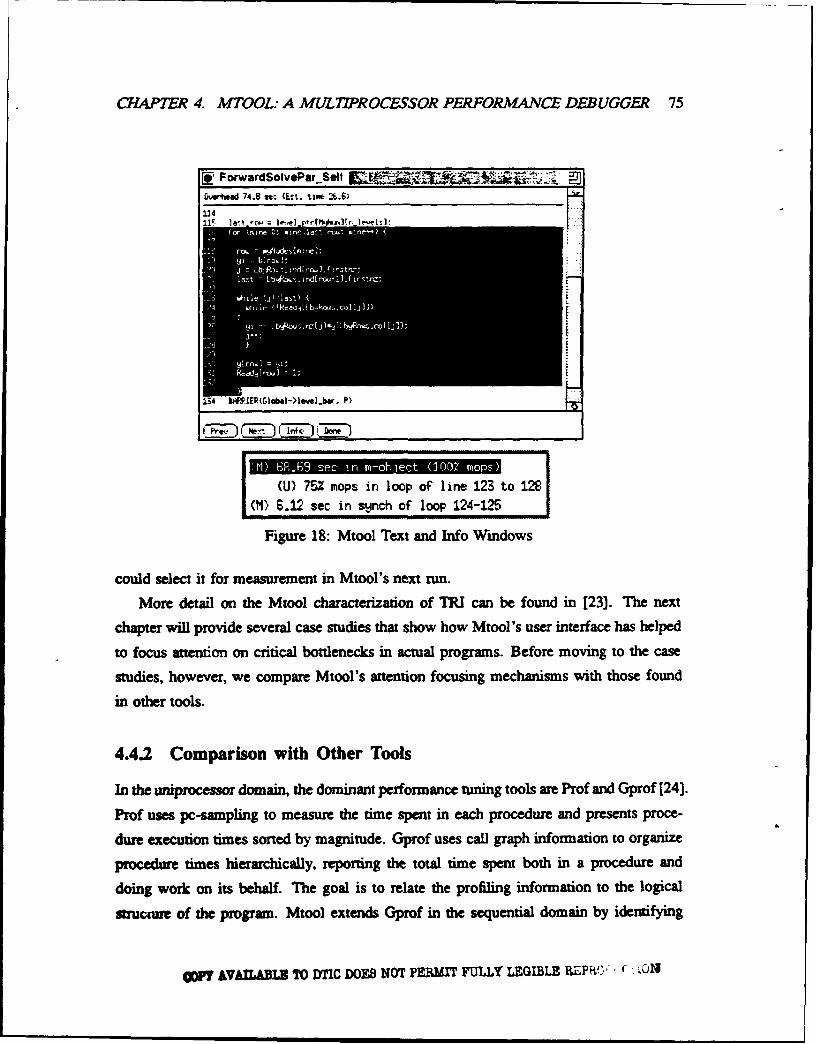
CHAPTER 4. MTOOL: A MULTIPROCESSOR PERFORMANCE DEBUGGER 75
Ee ForwardSolvefar_$ei j 4Dvpwhead 74.8 aec (Ent. tip* 216.6)114
11c:-~e Ia:]r
154 3.IERG Io.hi-eleve..b., P',
(U) 75% mops in loop of line 123 to 128
(Mi) 6.12 sec in smnch of loop 124-125 11Figure 18: Mtool Text and Info Windows
could select it for measurement in Mtool's next run.
More detail on the Mtool characterization of TRI can be found in [23]. The next
chapter will provide several case studies that show how Mtool's user interface has helped
to focus attention on critical bottlenecks in actual programs. Before moving to the case
studies, however, we compare Mtool's attention focusing mechanisms with those found
in other tools.
4.4.2 Comparison with Other Tools
In the uniprocessor domain, the dominant performance timing tools are Prof and Gprof [24].
Prof uses pc-sampling to measure the time spent in each procedure and presents proce-
dure execution times sorted by magnitude. Gprof uses call graph information to organize
procedure times hierarchically, reporting the total time spent both in a procedure and
doing work on its behalf. The goal is to relate the profiling information to the logical
structure of the program. Mtool extends Gprof in the sequential domain by identifying
My7 AVAIMLAZ To) DTIC DOWB NOT pEP.MIT FULLY LEGIBLE RPhEP'W - L1

CHAPTER 4. MTOOL: A MULTIPROCESSOR PERFORMANCE DEBUGGER 76
not only where a program is spending its time but also splitting this time into compute
time and memory system overhead. This additional information helps the user under-
stand the cause of the performance bottleneck, which guides the search for performance
enhancing transformations.
In the parallel domain, the emphasis of most tools aimed at shared address space
parallel programs is on distinguishing time spent doing work from time spent waiting
for work [2, 3, 5, 36, 42]. Despite the importance of memory system performance to
whole program performance, the tools neglect the distinction between time spent waiting
for data movement (memory system overhead) and actual computation. The tools do,
however, offer a variety of features for focusing attention on the nature and impact of
synchronization overhead. Below we review some of these features, describing how they
are supported in Mtool or why they were omited.
The Quartz system [2] uses "normalized processor time" as its primary attention
focusing mechanism:NPT f Tume Spent In Object
# of Processors Active While Object Executed
Quartz computes this metric by sampling with a dedicated processor that periodically
examines the call stack of each process in the program, recording the procedure the
process is executing and the number of other processes currently doing useful work. The
NVPT metric focuses attention on those procedures and synchronization objects most
critical to total execution time. The idea is that 1 second in sequential mode is as
important as 16 seconds aggregate time distributed over 16 simultaneously executing
parallel processes. Below we discuss the extent to which NPT is supported by Mtool.
For compiler parallelized Fortran, Mtool approximates Quarmz's normalized processor
time by dividing execution time into sequential time, normalized parallel time, and loop
overhead. More precisely, Mtool assumes that all processors are active in parallel mode,
measures total work in each parallel loop and wall clock time in parallel mode, and
computes:
= Work In Parallel Loop Loop Overhead = T.ne in Parallel Mode - .PT# of Processes
Parallel loops with significant load imbalance are highlighted by their large loop over-
heads.

CHAPTER 4. MTOOL: A MULTIPROCESSOR PERFORMANCE DEBUGGER 77
For the more complex ANL macro programming model, we cannot distinguish regions
of purely sequential and parallel execution. Thus, to measure NPT, Mtool must actually
sample average parallelism. The ideal sampling mechanism is the user level interrupt
service discussed in Section 4.2.1. Synchronization calls are instrumented to maintain
an active flag for each process. The active flag is set to false when a synchronization
object is entered and reset to true when the synchronization object is exited. If the active
flags are kept in global memory, then the user level interrupt handler that accomplishes
pc-sampling can both increment the bucket corresponding to the currently executing
instruction and note the number of active processes by examining the flags.
The advantage of the user level interrupt handler is that it eliminates the need to
make process-private information available to an external sampling process. In most
multiprocessor environments, the program counter and call stack of each process are in
process-private registers and memory. Hence, to profile a program with a dedicated sam-
pling process, the profiled program must be instrumented to write information about its
state to global memory. In Quartz, the program maintains a copy of its call stack in global
memory (at a reported 50% overhead), so only procedure level profiling information can
be gathered by the sampling processor. Because the user level handler can access local
process state, the overhead of maintaining a call stack in global memory is avoided and
a finer level profile can be collected..
Both NPT and aggregate execution time can help the user to recognize and under-
stand synchronization overhead in homogeneous parallel programs where all processes
are contending for a single lock or waiting at a single barrier. NPT will highlight the
contended for synchronization object and show that the code that is executing before the
synchronization call is a performance bottleneck. Similarly, sorting procedures and syn-
chronization objects by aggregate time will focus attention on the synchronization object
that is the subject of contention. But in more complex heterogeneous parallel programs
where processes have complicated event-driven interactions, aggregate time metrics like
NPT and total waiting time provide little insight into the sequence of events that caused
the synchronization bottleneck.
What is needed is the detailed information offered by trace-based tools like IPS-
2 [42]. These tools instrument a program to output time-stamped traces of events like

CHAPTER 4. MTOOL: A MULTIPROCESSOR PERFORMANCE DEBUGGER 78
procedure and synchronization object entries and exits. The traces allow post-processors
to reconstruct both the aggregate times spent in the loops and procedures, and to report
dynamic interprocess dependences (process 1 was waiting for the lock held by process
2). The IPS-2 system features a well-developed hierarchical user interface that provides
information on execution time and synchronization waiting time at the program, process,
procedure and synchronization object level. IPS-2 also offers guidance on where to
optimize by focusing attention on the critical path through the program. The problem
with IPS-2 and other trace-based tools is that they generate an enormous amount of data,
making it difficult to reduce their intrusiveness (and to physically store the data they
produce). Consider a program that spends most of its time executing a 2000 cycle leaf
procedure. If IPS-2 writes write a time-stamped event record of say 5 bytes each time the
procedure enters and exits, the instrumented program will produce 10 bytes of trace data
for every 2000 cycles of execution. On a multiprocessor with ten 20 MIPS processors,
the aggregate rate of data production will be around 100 Megabytes/second.
In general, trace-based tools can provide fine-grained information when Mtool's ag-
gregate characterization of synchronization or memory behavior is inadequate. If a certain
synchronization point has mysteriously long waiting times then selective tracing can be
used to understand that synchronization. However, because of its low perturbation, speed,
and ability to quantify memory effects, Mtool seems like a superior first-pass performance
debugging tool.
IPS-2 is notable not only for its critical path analysis facility, but also for its well
developed hierarchical user interface. Just as Gprof ties performance data to the logical
structure of the program by reporting times spent in a procedure and on its behalf, IPS-2
matches its performance data to the logical structure of the parallel program reporting data
at a whole program, process, procedure, and "primitive activity" level. The lowest level
typically corresponds to synchronization events. Mtool provides a similar hierarchical
model to help the user understand the parallel program's behavior.
In summary, Mtool's main attention focusing mechanisms are its hierarchical design
and its simple performance loss taxonomy. In addition, Mtool supports Quartz's .NPT
metric for ANL macro programs when user level pc-sampling is available, and uncondi-
tionally for Fortran programs parallelized by the compiler at the loop level. We elaborate

CHAPTER 4. MTOOL: A MULTIPROCESSOR PERFORMANCE DEBUGGER 79
on these mechanisms in the next chapter through a series of case studies.
Chapter 5
Case Studies
In this chapter, we provide examples that illustrate how programmers have used Mtool
to analyze and improve performance. We offer two full case studies and several excerpts
from performance debugging sessions. The first case study uses Mtool and SGI's Fortran
compiler to parallelize an economics simulation code. In only a few hours, through a
combination of memory overhead reduction and parallelization, the program's execution
time on an 8 processor SGI 380 was reduced from 5.5 minutes to 40 seconds. The second
case study describes porting a particle simulation to the 16 processor Stanford DASH
machine. Run-time is quickly improved 13% from 167 to 145 seconds and directions
for further improvement are suggested. Then, in Section 5.3 we give an example where
Mtool isolates a less common memory overhead, write buffer stalls. Finally, we show
how side by side comparisons of Mtool displays from sequential and parallel runs can
be useful in identifying sources of performance loss, particularly extra work introduced
by parallelization.
5.1 Fortran Case Study
The CARS program solves for the equilibrium price vector in a nested logit model with
230 vehicle types and 5000 household types [29]. The author of CARS needed to use it
as the main subroutine in a large simulation where CARS is called about 10,000 times.
The goal was to make the simulation run in under a week (so several scenarios could be
80

CHAPTER 5. CASE STUDIES 81
MTOOL: carsO (File is carsO),.- , ,,...,; -,..-':.?.: A:,::...
Total Seq Par
•'Est i. CPU Time: 169.81 169.81 0.00
lMemor4. Overhead: 151.99 151.99 0.00 measured 97% mops
CEx-i7t ) C Histograr_, ( CGRAPH .
Figure 19: Summary Window for CARSO
compared in a reasonable amount of time) which would require CARS to run in under
a minute. The original sequential version of CARS ran in 16 minutes when ported to
the SGI machine. Careful optimization of the program taking advantage of the structure
of the model produced a good baseline program, CARSO, with an execution time of
about 5.5 minutes. We used Mtool to study this program by executing the following five
commands.
mtool -BB carsO Instrument with counters.
cars0 .patch Run instrumented carsO to gather profile.
mtool -PF cars0 Using profile add timers and counters
cars O.mtool Run fully instrumented carsO.
show.rmtool carsO Invoke the user interface.
The show-atool command produced the top level summary window of Figure 19.
The window reports the total compute time and memory overhead measured when
cars0 .mtool was executed. In the bottom portion of the window, these times are
broken into time spent in sequential and parallel modes (for CARSO all time is sequen-
tial). The shaded horizontal bar in the top part of the window corresponds to the textual
information, with the length of the shaded regions proportional to the time spent in each
element of the performance loss taxonomy. The important point to note is that 152
seconds, or about half the program's execution time, is spent waiting on the memory

CHAPTER 5. CASE STUDIES 82
SHistogram (File carsO) 3 >.i#-
L C
S redicted
C 25-
Oer. 3oer der5der4 )d Ioop derl
Pr-mcueai~
Figure 20: Procedure Histogram for CARS0
hierarchy. Pressing the Histogram button provides a more detailed picture of where the
performance bottlenecks lie, producing the window of Figure 20
As described in Section 4.4.1, the bars of the histogram represent time spent in a
procedure and in calls on its behalf. The key in the upper left indicates that time is
divided into local (L) compute time, local memory overhead, compute time in calls
(C), and memory overhead in calls. From the histogram, it is evident that the proceduresdeI - der5 are responsible for the majority of execution time and memory overhead. In
fact, these five procedures have extremely similar structure and behavior, so we confine
our attention to the most compute intensive of them, der3. Moving the mouse over
the der3 bar and clicking produces a text window containing the source code of the
procedure as shown in Figure 21.
The highlighted region is a memory bottleneck. The top line of the window tells
us that this bottleneck is responsible for 49.1 seconds of memory overhead as compared
with an ideal compute time of 49.4 seconds. As described in Section 4.4.1, pressing Prey
and Next allows us to move to other bottlenecks within the procedure. Bottlenecks are
ordered by total time spent in the corresponding source code. Pressing the Info button
provides data on bottlenecks within the currently highlighted region.
CT AVAILABLE TO D DOES NOT PEI, IT FULLY LEGIBLE PEPODUCTIOV
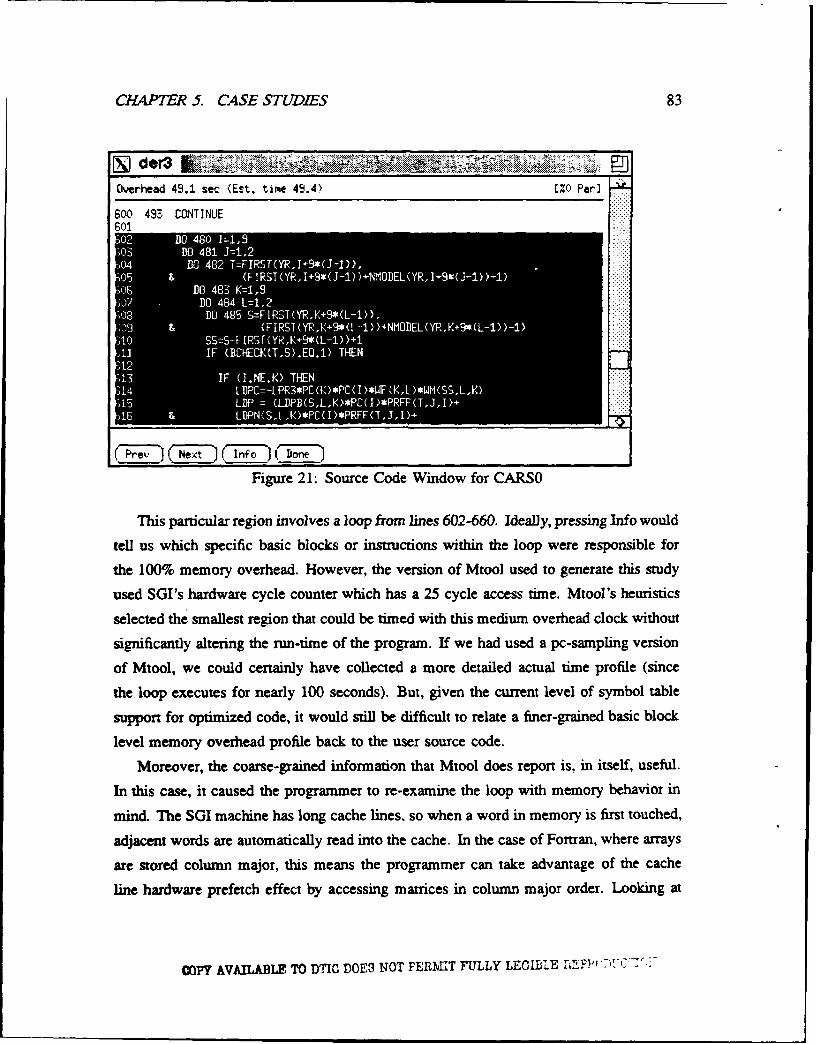
CHAPTER 5. CASE STUDIES 83
Sder3 ...............
Overhead 49.1 sec (Est. time 49.4) EZO Par)
600 493 CONTINUE601 ....
30 O48 z,
Figure 21: Source Code Window for CARS0
This particular region involves a loop from lines 602-660. Ideally, pressing Info would
tell us which specific basic blocks or instructions within the loop were responsible for
the 100% memory overhead. However, the version of Mtool used to generate this study
used SGI's hardware cycle counter which has a 25 cycle access time. Mtool's heuristics
selected the smallest region that could be timed with this medium overhead clock without
significantly altering the run-time of the program. If we had used a pc-sampling version
of Mtool, we could certainly have collected a more detailed actual time profile (since
the loop executes for nearly 100 seconds). But, given the current level of symbol table
supporn for optimized code, it would still be difficult to relate a finer-grained basic block
level memory overhead profile back to the user source code.
Moreover, the coarse-grained information that Mtool does report is, in itself, useful.
In this case, it caused the programmer to re-examine the loop with memory behavior in
mind. The SGI machine has long cache lines, so when a word in memory is first touched,
adjacent words are automatically read into the cache. In the case of Fortran, where arrays
are stored column major, this means the programmer can take advantage of the cache
line hardware prefetch effect by accessing matrices in column major order. Looking at
COPY AVAILABLE TO DTIC DOES N•OT PERMI?.T FULLY LEGiBLE IF• ........

CHAPTER 5. CASE STUDIES 84
MTOOL" cars1 (File is cars1)
Total Seq Par
;Estim. CPU Time: 169.81 169.81 0.00
*Memory Overhead: 54.34 54.34 0.00 measured 97% mops
Exit.] CHistogram-) (F GRAP H
Figure 22: Summary Window for CARSI
the source code window, we see the loops are nested in IJ,T,K,L,S order. In fact, every
significant array inside this sixty line loop is accessed in the appropriate column major
pattern with the single exception of the BCHECK(TS) access at line 611. It turns out that
BCHECK is an auxiliary data structure added during the initial sequential optimization
phase to store a pre-computed function of S and T. The array is actually symmetric so
we can replace BCHECK(TS) by BCHECK(ST) in each of the derl-der5 routines.
Making this change produces a new version of the program CARS 1. The summary
window produced when CARS 1 is run through Mtool is shown in Figure 22. Compute
time is, as expected, unchanged but memory overhead has dropped from 152 to 54 seconds
for about a 33% improvement in wall clock time. Mtool has focused our attention on
a loop with bad memory behavior, revealing a simple performance bug that was easily
repaired.
The next step is to run CARS 1 through the parallelizing compiler to create PCARSO.
Adding Mtool's instrumentation to PCARSO and running it on three processors produces
the disappointing display shown in the top portion of Figure 23. There are only 10.8
seconds of parallel time, 8 seconds spent computing and 2.8 seconds waiting on the
memory hierarchy. Note, these times have been normalized by the number of processors
to focus the user's attention on those parts of the program that contribute most to wall
clock time. For example, Mtool calculates the normalized parallel compute time as
Total Compute Time in Parallel Mode
Number of Processes

CHAPTER 5. CASE STUDIES 85
MTOOL: pcarsO (File is pcarso.3) L >
Total Seq Par
"r/Estim. CPU Timee: 153.33' 145.33 8.00EMtemor.y Overhead: 50.07 47.30 2.78 measured 94A mopsS Loop Overhead: 4.86 -
Exitx 1 Histogram- )CGRAPH
!J Histogram (File pcarso.3)
Ov &erhead
F Predicted
20 -
'EMA
oer3 oer . der, createvarder4 modloo derl ex
Proceoure
Figure 23: Summary Window and Procedure Histogram for PCARSO
so the 8 seconds of parallel compute time represent 24 seconds of total compute time
executed on 3 processors.
It is obvious from the textual portion of the summary window in Figure 23 that
sequential execution mode is dominating the run-time. Pressing the Histogram button
produces the window in the bottom part of Figure 23. There are two bars associated with
each procedure: the left bar corresponds to sequential time (including loop overhead)
and the right bar corresponds to normalized parallel time (i.e., aggregate work in parallel
To 2..C -Z, tjT L
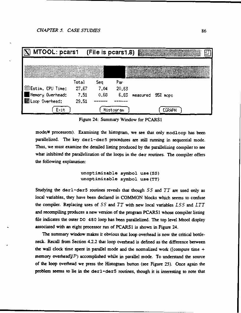
CHAPTER 5. CASE STUDIES 86
WOOL pcarsl (File is pcarsi.8)
Total Seq Par.
SEst i m. CPU Time: 27.67 7.04 20.63* emorq Overhead: 7.51 0.68 6.83 measured 95% mops
SLoop Overhead: 29.51
(Exit . HistoArar;, CGF-.PH]
Figure 24: Summary Window for PCARS 1
mode/# processors). Examining the histogram, we see that only modloop has been
parallelized. The key derl-der5 procedures are still running in sequential mode.
Thus, we must examine the detailed listing produced by the parallelizing compiler to seewhat inhibited the parallelization of the loops in the der routines. The compiler offers
the following explanation:
unoptimizable symbol use(SS)unoptimizable symbol use(TT)
Studying the derl-der5 routines reveals that though SS and TT are used only as
local variables, they have been declared in COMMON blocks which seems to confuse
the compiler. Replacing uses of SS and TT with new local variables LSS and LTTand recompiling produces a new version of the program PCARS1 whose compiler listing
file indicates the outer DO 4 8 0 loop has been parallelized. The top level Mtool displayassociated with an eight processor run of PCARS1 is shown in Figure 24.
The summary window makes it obvious that loop overhead is now the critical bottle-
neck. Recall from Section 4.2.2 that loop overhead is defined as the difference between
the wall clock time spent in parallel mode and the normalized work ([compute time +
memory overhead]!P) accomplished while in parallel mode. To understand the source
of the loop overhead we press the Histogram button (see Figure 25). Once again the
problem seems to lie in the derl-der5 routines, though it is interesting to note that
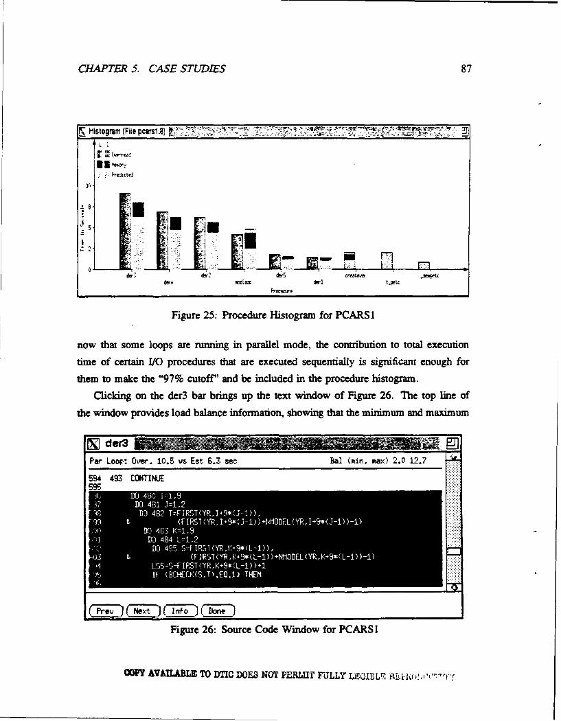
CHAPTER 5. CASE STUDL)ES 87
H iastogram (File pcarsi.sJ W"Lt
r rod;
L-J
dw dr m. dr dr m t tejc
srt
Figure 25: Procedure Histogram for pCARS1I
now that some loops are running in parallel mode, the contribution to total execution
time of certain 1/0 procedures that are executed sequentially is significant enough for
them to make the "97% cutoff" and be included in the procedure histogram.
Clicking on the der3 bar brings up the text window of Figure 26. The top line of
the window provides load balance information, showing that the minimum and maximum
~der3
Par Loop: Over. 10.5 vs Est 6.3 see Dal (min, max) 2. 0 IL, .7
594 493 CONTINUE59c5
DO4I J=1,DO42T=IS(Ys+*
9 & F IST YR,1+9 (J1))+NHD:-L (P, +Ct*(-1) -1
DO 483 K71,9
Fiur 26: Sorc Cod Windo fo PCAoRD=or
COPY AVAILABL TO DTIC DOES NOT PERMIT FULLY' LEGIBLr, ("''
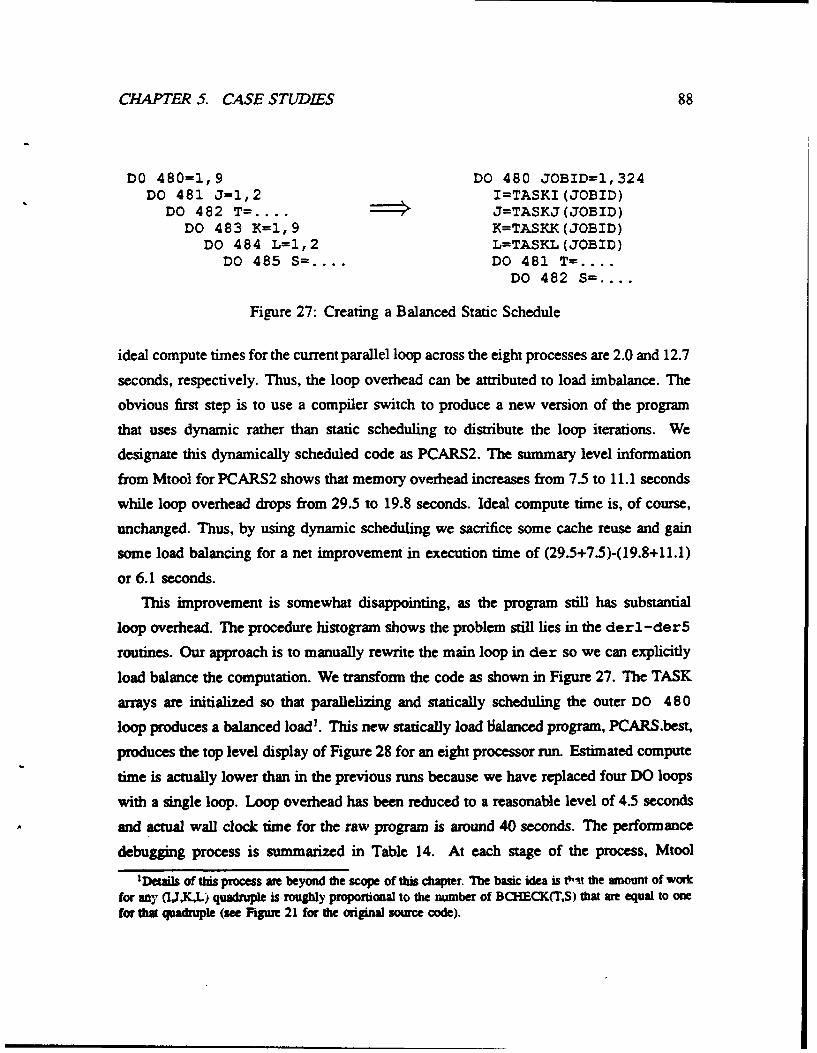
CHAPTER 5. CASE STUDIES 88
DO 480=1,9 DO 480 JOBID=1,324DO 481 J=1,2 I=TASKI (JOBID)
DO 482 T= .... J=TASKJ(JOBID)DO 483 K=1,9 K=TASKK (JOBID)
DO 484 L=1,2 L=TASKL(JOBID)DO 485 S= .... DO 481 T=....
DO 482 S= ....
Figure 27: Creating a Balanced Static Schedule
ideal compute times for the current parallel loop across the eight processes are 2.0 and 12.7
seconds, respectively. Thus, the loop overhead can be attributed to load imbalance. The
obvious first step is to use a compiler switch to produce a new version of the program
that uses dynamic rather than static scheduling to distribute the loop iterations. We
designate this dynamically scheduled code as PCARS2. The summary level information
from Mtool for PCARS2 shows that memory overhead increases from 7.5 to 11.1 seconds
while loop overhead drops from 29.5 to 19.8 seconds. Ideal compute time is, of course,
unchanged. Thus, by using dynamic scheduling we sacrifice some cache reuse and gain
some load balancing for a net improvement in execution time of (29.5+7.5)-(19.8+11.1)
or 6.1 seconds.
This improvement is somewhat disappointing, as the program still has substantial
loop overhead. The procedure histogram shows the problem still lies in the derl-der5
routines. Our approach is to manually rewrite the main loop in der so we can explicitly
load balance the computation. We transform the code as shown in Figure 27. The TASK
arrays are initialized so that parallelizing and statically scheduling the outer DO 480
loop produces a balanced loads. This new statically load balanced program, PCARS.best,
produces the top level display of Figure 28 for an eight processor run. Estimated compute
time is actually lower than in the previous runs because we have replaced four DO loops
with a single loop. Loop overhead has been reduced to a reasonable level of 4.5 secondsand actual wall clock time for the raw program is around 40 seconds. The performance
debugging process is summarized in Table 14. At each stage of the process, Mtool1Details of this process ae beyond the scope of this chapter. The basic idea is t0-t the anount of work
for any (IJK,L) quadruple is roughly proportional to the number of BCHECK(TS) that are equal to onefor that quadruple (see Figum 21 for the original source code).
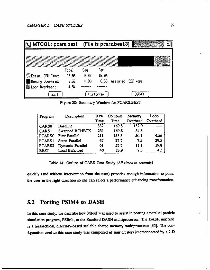
CHAPTER 5. CASE STUDIES 89
W[• M OOL' pcars.best (File is pcars.best.8) LN•~i•V~ •• gD
Total Seq Par
•Estir. CPU Time: 23.931- 6.97 16.95*riemory Overhead: 9.33 0.80 8.53 measured 92% mops
ILoop Overhead: 4.54 .... ...
(7yi -t Historam) ( CGRAPH
Figure 28: Summary Window for PCARS.BEST
Program Description Raw Compute Memory LoopTime Time Overhead Overhead
CARSO Baseline 332 169.8 152.0CARSI Swapped BCHECK 231 169.8 54.3PCARSO First Parallel 211 153.3 50.1 4.86PCARS1 Static Parallel 67 27.7 7.5 29.5PCARS2 Dynamic Parallel 61 27.7 11.1 19.8BEST Load Balanced 40 23.9 9.3 4.5
Table 14: Outline of CARS Case Study (All times in seconds)
quickly (and without intervention from the user) provides enough information to point
the user in the right direction so she can select a performance enhancing transformation.
5.2 Porting PSIM4 to DASH
In this case study, we describe how Mtool was used to assist in porting a parallel particle
simulation program, PSIM4, to the Stanford DASH multiprocessor. The DASH machine
is a hierarchical, directory-based scalable shared memory multiprocessor [35]. The con-
figuration used in this case study was composed of four clusters interconnected by a 2-D
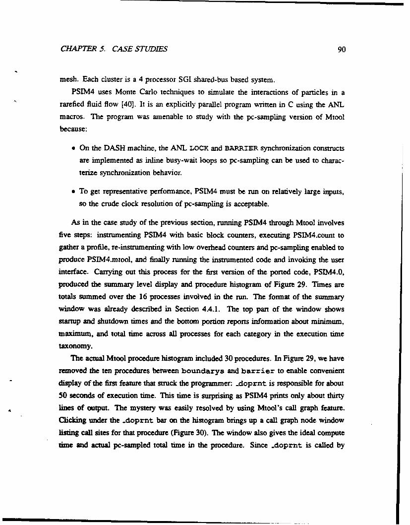
CHAPTER 5. CASE STUDIES 90
mesh. Each cluster is a 4 processor SGI shared-bus based system.
PSIM4 uses Monte Carlo techniques to simulate the interactions of particles in a
rarefied fluid flow [40]. It is an explicitly parallel program written in C using the ANL
macros. The program was amenable to study with the pc-sampling version of Mtool
because:
"* On the DASH machine, the ANL LOCK and BARRIER synchronization constructs
are implemented as inline busy-wait loops so pc-sampling can be used to charac-
terize synchronization behavior.
"* To get representative performance, PSIM4 must be run on relatively large inputs,
so the crude clock resolution of pc-sampling is acceptable.
As in the case study of the previous section, running PSIM4 through Mtool involves
five steps: instrumenting PSIM44 with basic block counters, executing PSIM4.count to
gather a profile, re-instrumenting with low overhead counters and pc-sampling enabled to
produce PSIM4.mtool, and finally running the instrumented code and invoking the user
interface. Carrying out this process for the first version of the ported code, PSIM4.0,
produced the summary level display and procedure histogram of Figure 29. Tunes are
totals summed over the 16 processes involved in the run. The format of the summary
window was already described in Section 4.4.1. The top pan of the window shows
startup and shutdown times and the bottom portion reports information about minimum,
maximum, and total time across all processes for each category in the execution time
taxonomy.
The actual Mtool procedure histogram included 30 procedures. In Figure 29, we have
removed the ten procedures between boundarys and barrier to enable convenient
display of the first feature that struck the programmer: _doprnt is responsible for about
50 seconds of execution time. This time is surprising as PSIM4 prints only about thirty
lines of output. The mystery was easily resolved by using Mtool's call graph feature.
Clicking under the .doprnt bar on the histogram brings up a call graph node window
listing call sites for that procedure (Figure 30). The window also gives the ideal compute
time and actual pc-sampled total time in the procedure. Since _doprnt is called by

CHAPTER 5. CASE STUDIES 91
SMTOOL: psim4.0 (File is verO.16) . •''
Time for Master (sec) Time0 36 7' 108 144
Total: 175.00Startup: 1. 00 Master
Shutdown: 0.00 S I avel
Slave15
Total Mir, Max•Estim. CPU Time: 1510.39 92.85 95.85*Memory Overhead: 627.19 35.78 47.20 measured 90% mops
SSynch Overhead: 463.02 20.36 34.30
Sys Time: 20.78 0.87 2.56- Par. Overhead: 0.62 0.03 0.06
SEx 3 ( Histograr, 3 ( CGRAPH 3
Sttutogram (Fits vuO.16) -
QC Est. Cft (sr. kids'
i • Eat. CPU
260.
Figure 29: Summary Window and Histogram for PSIM4.0
~J I ~ U ~]1.44 sec. (act)L5.39 sec (act) Iai 0.59 sec (cpu)
33.27 sec (cpu) Called 672820 Times N: Line %Called 673051 Times B: Line X putt_particle 282 100
iprlntf 49 100 Z Work in Kids.doprnt: 98
Figure 30: Call Graph Nodes for .doprnt and sprintf
OPY AVAILABL TO DTIO DOES NOT PERMIT FULLY" LEGIBLE tEPRuOa i'r I0u

CHAPTER 5. CASE STUDIES 92
sprintf, we bring up its call graph node as well (by pressing the CGRAPH button at
the bottom of the summary window).
It turned out that the programmer had removed some debugging print statements, but
had inadvertently forgotten to delete an sprint f call that formatted strings containing
debugging information. Mtool's call graph feature immediately guided the programmer
to the problem and it was eliminated to create a new version of the program PSIM.l.
The top level display and procedure histogram for PSIM.1 are shown in Figure 31. (In
the procedure histogram, bars to the right of psimufree have been deleted.)
The summary window shows that compute time has dropped from 1510 to 1476
seconds which corresponds to the removal of the 34 seconds spent in sprint f and
.doprnt. Memory overhead has dropped by 36 seconds which is a bit more than the
19 second overhead attributed to .doprnt, but not so large as to be implausible. The
dramatic improvement is in synchronization overhead which has been reduced by nearly
150 aggregate seconds. The apparent explanation is that the _doprnt call lay along the
critical path of the program so removing it eliminated idle time elsewhere. (In fact, it is
clear from the full procedure histograms that a certain barrier was a significant bottleneck
in PSIM.0 and removing the _doprnt call has eliminated the waiting time at this barrier.)
With the obvious performance "bug" eliminated, the next bottleneck that grabbed
the programmer's attention was the synchronization overhead in ps im-free. Clicking
on the bar produced the source code window of Figure 32 with the lock of line 195
highlighted. The top line of the source code window tells us that 72.9 total seconds
are spent contending for this lock. The problem arises because psim-free is a central
global memory management routine, and all processes in the computation need to free
memory at about the same time. Once Mtool highlighted the bottleneck, the programmer
replaced the central memory manager with a distributed scheme: each processor is given
a large chunk of global memory to allocate locally. The local memory management
version, PSIM4.2, reduced synchronization overhead by 102 seconds with no significant
changes in compute time or memory overhead. Note, this 102 second improvement
exceeds the 73 seconds that had been spent contending for the lock in psim-free.
The extra improvement is not surprising as the top line of the source code window in
Figure 32 shows that some process waited on the lock only 0.8 seconds while another
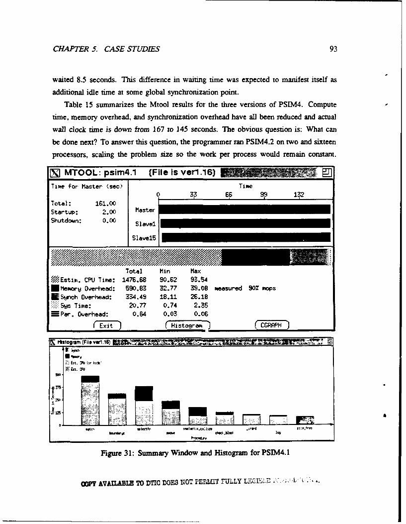
CHAPTER 5. CASE STUDIES 93
waited 8.5 seconds. This difference in waiting time was expected to manifest itself as
additional idle time at some global synchronization point.
Table 15 sumnmarizes the Mtool results for the three versions of PSIM4. Compute
time, memory overhead, and synchronization overhead have all been reduced and actual
wall clock time is down from 167 to 145 seconds. The obvious question is: What can
be done next? To answer this question, the programmer ran PSIM4.2 on two and sixteen
processors, scaling the problem size so the work per process would remain constant.
~jMTOOL: psim4.1 (File is verl.16) ~ ~
Time for Master (sec) Time0 33 66 99 132
Total: 161.00Startup: 2.00 MasterShutdowun: 0.0'0 Slavel
SI ave15
Total Min MaxM',Estim. CPU Time: 1476.68 90.62 973.54*Memori~j Overhead: 590.83, 32.77 39.08 measured 90Z mopsKESýnch Overhead: KU3.449 18.11 26.18
*Sly-s T ime: 20.77 0.74 2.35~Par. Overhead: 0.64 0.03 0.06
r -Exit 7 ( Histogram -) CCGRA-PH I
Es.t 71):ir kt*
Ea ~. 0:
f 7M
"7,th Ifn w. .o I icFTrdud ..IObloCl log
Figure 3 1: Summary Window and Histogram for PSIM4.1
MOY AVAILABLE TO DTIC DOES NOT~ PEPIMIFULLY LECGtL1 7:~ L~

CHAPTEJR 5. CASE STUDIES 94
Program Description Raw Compute Memory SynchronizationTime Time Overhead Overhead
PSIM4.0 Baseline 167 1510 627 483PSIM4.1 Removed sprintf 157 1476 591 334PSIM4.2 Fixed psim...free 145 1476 600 232
Table 15: Summary of PSIM4 Case Study (All times in seconds)
This scaling is achieved by linearly scaling the input data size. The average per process
compute times, memory overheaes, and synchronization overheads are given in the next
table.
Tunes Per Processor (seconds)
Compute Memory Synch
2 Processors 92 28 1
16 Processors 92 38 15
This simple table is important because it helps the programmer to determine how to im-
prove performance. Recall the problem was scaled by linearly increasing the input size.
For PSIM4, this means the amount of data per processor is nearly constant in the two and
IJ psimjfree EllS.,ch Idle Time (sec): 72.9 Dal (mirn, ex) 0.8 EF.5185 void psim.free(ptr, type)196 char *ptr;187 int type"188 {189 *ifdef DEBUG190 pdebug(l, *psimfree", "enter");191 *endif192 if (type = PRIVATE) {193 free(pitr):194 else if (tye == SHARED) {
196 G.FREE'•ptr.'* 197 UNHLOCK (Wm?mem_ Ilock)
198 } else {
Figure 32: Source Code Window for PSIM4.1

CHAPTER 5. CASE STUDIES 95
sixteen processor runs. If there were no intercluster communication, we would expect
similar memory overheads per process in each run. In fact, the memory overheads are
38 and 28 sec.nds respectively. A reasonable hypothesis is that at most 10 seconds per
process is being lost to intercluster communication. The rest of the memory overhead is
inherent in the single cluster implementation of PSIM4. This observation is important
because it prevents the programmer from wasting time trying to use DASH's software
prefetch to improve performance. The prefetch operation transfers data between clusters,
leaving the fetched data in a cluster level cache so it is only applicable to hiding the
latency of intercluster memory transfers. For PSIM4.2, the programmer will need opti-
mizations that either improve single cluster memory behavior or reduce synchronization
overhead. By explicitly separating out compute time, memory overhead, and synchro-
nization overhead, Mtool has focused the programmer's attention on the high-level nature
of the next bottlenecks to correct.
5.3 Write Buffer Effects
One motivation for building Mtool was to help the programmer to cope with the growing
complexity of memory systems. This section describes a lower level memory system
feature that hindered performance during an attempt to optimize the c shift procedure
in the water code from the SPLASH suite. A full description of the case study may be
found in [22].
Running the water code through Mprof identified cshift as a performance criti-
cal procedure. The routine was subsequently recoded in assembly to optimize register
allocation. The performance of the C and assembly coded versions of water are shown
in Table 16. Recoding in assembly improves ideal compute time by 20%, but actual
execution time is reduced by less than 4%. Somehow, the assembly coded routine has
encountered a memory bottleneck. At first this result was puzzling as the only differ-
ence between the C and assembly versions of cshift is that some redundant address
computations and load operations have been eliminated. The optimized assembly con-
sists of a long sequence of subtractions and stores. Discussions with the local hardware
experts revealed the problem. The SGI cache can retire one store every two cycles but

CHAPTER 5. CASE STUDIES 96
the program is generating two stores every three cycles. While there is a store buffer of
depth four to handle bursts, the architects did not design the hardware to service (without
stalling) a program with such high sustained store bandwidth. Though Mtool did notsay, "This is a store buffer problem," it gave enough information so a question could be
posed to experts.
5.4 Side by Side Comparison
Let us consider what happens when we compare Mtool profiles for single and multipleprocessor runs of the same program. If the program experiences perfect speedup, thenthe total compute time, memory overhead, and synchronization overhead, summed across
all processes in the multiprocessor run will match those from the single processor run.Mtool's hierarchical user interface permits a simple side by side comparison of the two
runs to determine exactly wnere and why performance is being lost. As suggested inSection 4.3, such comparisons are particularly helpful in isolating extra work due toparallel overhead. Below we offer an actual example of how the Power Fortran compilerintroduced extra work by making a poor choice about which loop to parallelize. We also
show how side by side comparison can provide insight into how to further improve the
CARS program of Section 5.1.
The nvst program solves a 3-D Navier Stokes equation on a composite grid. Itis a Fortran program parallelized by the compiler. To check for extra work due toparallelization, we disabled processor time normalization in the Mtool user interface andcompared the top level Mtool displays for one and four processor runs of nvst. We found
ideal compute times of 144 and 191 seconds respectively. The procedure level histograms
Version CPU Memory TotalTime Overhead Time
C Language 24 3 27Assembly 20 6 26
Table 16: cahift Performance (Aggregate Times in Seconds)
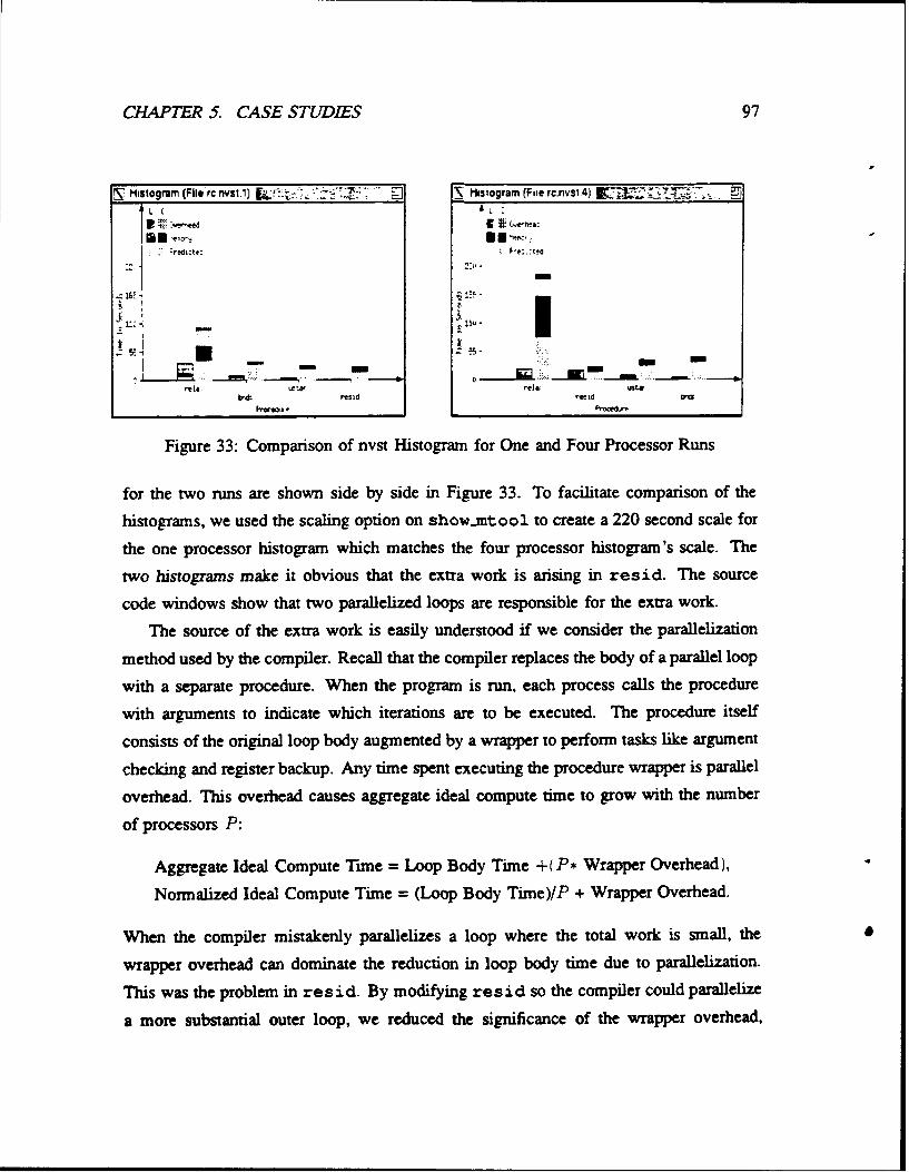
CHAPTER 5. CASE STUDIES 97
S. Histogram (File rc nstJ j.1 > Q Histogram (File Tc nvsl4) V7W ~L C L
: :redcte: F-e..:ted
"1. -" I
r~eltetr elw Ustkr4: FPwo rsid raid Prm* w
Figure 33: Comparison of nvst Histogram for One and Four Processor Runs
for the two runs are shown side by side in Figure 33. To facilitate comparison of the
histograms, we used the scaling option on show.mtool to create a 220 second scale for
the one processor histogram which matches the four processor histogram's scale. The
two histograms make it obvious that the extra work is arising in resid. The source
code windows show that two parallelized loops are responsible for the extra work.
The source of the extra work is easily understood if we consider the parallelization
method used by the compiler. Recall that the compiler replaces the body of a parallel loop
with a separate procedure. When the program is run, each process calls the procedure
with arguments to indicate which iterations are to be executed. The procedure itself
consists of the original loop body augmented by a wrapper to perform tasks like argument
checking and register backup. Any time spent executing the procedure wrapper is parallel
overhead. This overhead causes aggregate ideal compute time to grow with the number
of processors P:
Aggregate Ideal Compute Tune = Loop Body Time +( P* Wrapper Overhead),
Normalized Ideal Compute Time = (Loop Body Time)/P + Wrapper Overhead.
When the compiler mistakenly parallelizes a loop where the total work is small, the
wrapper overhead can dominate the reduction in loop body time due to parallelization.
This was the problem in resid. By modifying resid so the compiler could parallelize
a more substantial outer loop, we reduced the significance of the wrapper overhead,

CHAPTER 5. CASE STUDIES 98
SHistogram (File best l tot) V :
- L
Predicted
"I , •45
der. der Ier wd o rd 5d rlU rie
L Histogram (File best.8.tot) iL [ • :Air• .. t• .. _
L I., I, I
o.. . (./,, _ i,4. ,._ i ,-.T••,, -__ --.- * , ,.. .--die: der: aer5 exs
fin"ndo dnoetv
j~~tga Filue 34:..tt Coprsno HsormfrOn n ih PoesrRn
SPredicted
30 -
der3 der der. do dn eS rae
Figure 34: Comparison of Histogram for One and Eight Processor Runs
eliminating the parallel overhead and achieving near perfect speedup for the procedure.
The CARS program described earlier in this chapter offers another example of the
importance of side by side comparison. All Mtool displays in the CARS study used
the NPT time metric to focus attention on performance bottlenecks. However, while
.VPT is important for highlighting where performance bottlenecks lie, raw aggregate
time (summed over all processes) can often provide additional insight into why perfor-
mance is being lost. Figure 34 shows aggregate time procedure histograms for one andeight processor runs of PCARS.best. Comparing the two histograms, it is clear that an
important cause of imperfect speedup is an increase in memory overhead in the mod0oop
procedure. Somehow, locality is being lost in the eight processor run, and this situation
must be corrected if the programmer wants better performance. When only normalized

CHAPTER 5. CASE STUDIES 99
time is displayed, it is difficult to make this kind of comparison between runs on differ-
ent numbers of processors. We believe side by side comparison of aggregate times is an
important technique for identifying performance bottlenecks.
0

Chapter 6
Conclusions
In this dissertation we have presented an integrated framework for using low overhead
software instrumentation to characterize the run-time performance of parallel programs
on shared address space machines.. Our framework, which is based on dynamic basic
block counts and actual execution time data, offers three distinct advantages:
1. By utilizing profile information, we can estimate and control the overhead of our
instrumentation, typically slowing programs by less than 10%.
2. By comparing actual and ideal compute times, we are able to quantify the effect of
the memory system on performance (without simulating the memory hierarchy).
3. By providing a simple, hierarchical user interface, we enable the programmer to
navigate and understand the often tremendous amounts of data that are collected
by the instrumentation.
The first two advantages exploit the information available in the basic block count profile.
In particular, by examining the frequency with which a basic block is executed we can
select interesting portions of the program to instrument automatically, keeping timer0 overhead to acceptable levels and collecting basic block counts inexpensively. Further,
the basic block counts and a pipeline model allow us to derive the ideal compute time
profile of the program. Finer level information on floating point stalls and register usage
can also be extracted using this technique.
100
CHAPTER 6. CONCLUSIONS 101
To demonstrate the effectiveness of our performance tuning system, we implemented
the Mtool prototype. Mtool's user interface is well-matched to the programmer's model,
reporting bottlenecks in terms of the procedures, loops and synchronization objects that
make up a program. Execution time is divided into categories that naturally correspond to
different optimization approaches: compute time, memory overhead and synchronization
overhead. While we consider Mtool successful both as a "proof of concept" of the above
advantages and as the actual performance debugging environment for programmers of
SGI multiprocessors and the DASH machine, we recognize that substantial research
remains be done. In the next section, we describe some limitations in Mtool's approach
to understanding memory behavior. In the final section, we consider directions for further
research.
6.1 Mtool Limitations
Mtool isolates memory overhead by comparing ideal and actual execution times, iden-
tifying the source code lines where the overhead is incurred. Below, we discuss three
situations where this source code orientation may be inappropriate.
Code with Time Varying Behavior
Sometimes there is significant variation in the run-time behavior of a procedure de-
pending on the conditions under which it is called. Since Mtool records only aggregate
profile information about each basic block (e.g., total number of times the block is exe-
cuted), it can only determine the average memory system performance of each procedure.
This aggregate overhead may not adequately highlight the specific conditions under which
the overhread arises (e.g., the particular procedure arguments). In some cases, it may
be possible to capture argument dependent effects by collecting profile information on a
per call-site basis. Thus, we could modify Mtool to maintain a private set of counts and
times for each possible call-site of the procedure as discussed in Section 2.3 and then
report the compute time and memory overhead of the procedure on behalf of each call
site. However, in general, the behavior of the procedure may vary over time or program
phase, even when called from a single site. To capture time varying effects, Mtool would
have to dump its profile counts and times periodically, collecting a sequence of memory

CHAPTER 6. CONCLUSIONS 102
overhead profiles to describe a single program execution.
One Bottleneck Containing Multiple Data Objects
Many loops and procedures access more than one data object. In principle, Mtool
can use pc-sampling to measure the aggregate execution time of each individual memory
access instruction in a loop and then report exactly which accesses result in substantial
memory overhead. In practice, the actual time profile is often too crude to pick out which
memory accesses are the bottleneck. Mtool can only isolate bottlenecks to the level of
specific instructions when the user selects a long running input.
Diffuse Memory Overhead
Occasionally, the interaction of multiple procedures creates a memory bottleneck.
While Mtool can tell the programmer that procedures, fool, foo2, and foo3 all involve
100% memory overheads, it will not indicate that it is the interaction of these three
procedures that collectively create a bottleneck for the memory system. The problem
here is that to understand the cause of the bottleneck, the user needs data-object-oriented
rather than code-oriented performance information.
Of the three problems mentioned above, only the final problem of diffuse memory
overhead seems beyond the realm of Mtooll. Despite this limitation, Mtool has proven
quite useful in practice. We believe Mtool's effectiveness derives from two trends:
1. Memory bottlenecks that are easy to reduce usually result from an obvious mis-
match between the data access pattern and the actual memory system implementa-
tion. Simply knowing a code segment has abysmal memory system performance
often allows the user to guess that something simple like direct map cache conflicts,
false sharing, or poor access stride is at fault.
2. Mtool's technique for isolating memory overhead is independent of the actual
memory hierarchy. As the complexity of memory hierarchies and their impact
on performance grows, it will become increasingly important to distinguish mem-
ory overhead from compute time in a manner that is independent of the memory
system.
'Work to collect data-oriented information using simulation and hardware instrumentation is describedin [39]

CHAPTER 6. CONCLUSIONS 103
Thus, we feel that comparing actual and ideal compute times is a powerful "first-pass"
technique for characterizing the nature of a program's performance bottleneck.
One other potential limiting factor for Mtool is our ability to derive ideal compute
times for future architectures. Our derivation of ideal compute time relies on the as-
sumption that instruction latencies are static and fixed. For speculative architectures with
dynamic scheduling this assumption is not immediately satisfied. Thus, in the future
we may need more detailed simulation to establish a range of ideal compute times for
a sequence of instructions, and then we may only be able to offer an estimated range
for memory system overheads. Despite this need for approximation, we expect the basic
notion of comparing actual and ideal compute times to remain relevant. Motivated by this
expectation, we discuss below our plans to generalize and extend the Mtool methodology.
6.2 Further Research
The most obvious way to extend Mtool is to port it to other RISC microprocessor based
platforms. We hope to add support for the SPARC, Intel 1860, and IBM RS6000 chips in
the near future. In the sections that follow, we suggest some more ambitious extensions
to Mtool.
6.2.1 Attention Focusing and Feedback-Based Code Transformation
The goal of a performance tuning environment is to describe the cause of performance
bottlenecks in as much detail as possible. One natural way to improve Mtool's attention
focusing in loop oriented code is to use static compiler analysis to highlight arrays that
are accessed inefficiently. We would like to integrate the static analysis-based tools
described in Chapter 1 into the Mtool environment. Such tools could, for example, flag
the BCHECK array access in the CARS case study (Figure 21) as the likely cause of the
memory bottleneck there.
A second natural way to improve attention focusing is to automate the side-by-side
comparison technique described in Section 5.4. Ideally, Mtool would maintain a database
of profiles, automatically searching the database for particular procedures that do not

CHAPTER 6 CONCLUSIONS 104
speed up linearly and highlighting the elements of the execution time taxonomy respon-
sible for the lack of speedup in these procedures.
Ultimately, we hope to improve Mtool's attention focusing to the point where the user
can be removed from the loop. That is, we would like Mtool to describe performance
bottlenecks so precisely that a compiler can improve performance automatically. One
simple application of profile information is to guide a compiler in selecting the best
scheduling algorithm for fully parallel loops. A compiler may, for example, initially
default to static scheduling for a loop; then, when Mtool reports the loop has poor load
balancing behavior the compiler can switch to dynamic scheduling. Further feedback
can be used to refine the choice of dynamic scheduling algorithm. More ambitiously,
we would like to exploit the Mtool profile to guide the placement of prefetch operations,
drive the selection of unimodular loop transformations, and even suggest the need for
changes in the layout of data.
6.2.2 Selective Tracing
As discussed in Section 4.4.2, in complicated heterogeneous parallel programs it is some-
times necessary to understand the dynamic interactions of the tasks. Aggregate profile
information is inadequate to characterize these dynamic interactions and we must collect
time-stamped event traces. Similarly, to understand complex memory system behavior, it
is occasionally necessary to trace and then later resimulate the stream of memory refer-
ences. Of course, the drawback of trace based systems is their tendency to generate too
much data. We are optimistic that the Mtool principle of exploiting a previous profile to
guide selective instrumentation can be applied to control the amount of data generated
when tracing.
6.2.3 Exploiting Hardware Instrumentation
In the introduction, we noted the advantage of hardware instrumentation is its ability
to collect fine-grained data non-intrusively. Below, we briefly describe several forms of
instrumentation that would enhance Mtool's functionality. In some cases, the hardware
instrumentation is already available in selected systems.
CHAPTER 6 CONCLUSIONS 105
" High Resolution Timers: The importance and applicability of a high resolution,
low overhead timer for actual time profiling is discussed in detail in Sections 2.4
and 4.2.1.
"* Instrumented Memory Hierarchy: Mtool could more precisely characterize
memory overhead by associating specific memory hierarchy utilization informa-
tion with measured bottlenecks in the program. In particular, we would like to
have counters and timers so we can record the bus waiting time, cache miss rates,
TLB miss rates, etc.2 both for particular code segments and for data objects (mem-
ory address ranges). Such hardware is available in the DASH prototype and we
hope to extend Mtool to exploit it.
" Support for Tracing When we want to trace events like procedure entry/exit or
synchronization object acquisition/release, it is useful to have a special coprocessor
so that a single coprocessor instruction can be used to generate a time-stamped event
with a specified event identifier.
" Support for Sampling As discussed in Sections 4.2.1 and 4.4.2, it is highly de-
sirable for a system to provide a sampling interrupt to user level processes. Then,
custom user level handlers can be written to perform functions like charging the
time spent in synchronization routines to call sites and measuring average paral-
lelism. Similarly, when performance debugging the operating system, it is useful
to have separate pc-sampling and wall clock time interrupts so that we can apply
pc-sampling to the operating system.
To conclude, as computer systems become increasingly sophisticated and worst case
memory latencies grow, we need to improve the tools that help us to understand how
well a program is being mapped to a particular machine. Ultimately, the tools that
characterize run-time performance must be enhanced to the point where the user can be
removed from the loop and the compiler and run-time system can automatically improve
the match between the program and the computer system on which it is being executed.
21n some cues, it may be helpful to instrument the operating system as well as the hardware; forexample, when TL.B misses are handled in softwmae.

Appendix A
Mprof Results for the SPECmarks
This Appendix contains the output of Mprof for each of the SPEC benchmarks. The
benchmarks were compiled at the -02 level using version 2.1 of the SGI compilers and
executed on a single processor of an SGI 380 running IRIX 4.0. The latter part of the
appendix briefly discusses the memory overhead in the five SPECmarks whose CPU
utilizations are 75% or more. Detailed discussions of the other five SPECmarks may be
found in Chapter 2.
matrix300
CPU Utilization 25.5% (Actual Tume 338.0 vs Compute Time 86.2))
PROCEDURE NAME % Actual Time Tune in Sec. CPUNet Mem Comn Mere Corn Uti]
saxpy_ 99.5 74.2 25.3 250.8 85.5 25.4Loop from 429 to 430 97.3 73.1 24.2 247.0 81.8 24.9
106

APPENDIX A. MPROF RESULTS FOR THE SPECMARKS 107
nasa7
CPU Utilization 30.9% (Actual Time 1110.8 vs Compute Time 343.7))
PROCEDURE NAME % Actual Time Time in Sec. CPUNet Mem Corn Mern Corn Util
vpenta_ 25.8 22.5 3.2 250.5 35.8 12.5
Loop from 1095 to 1104 8.5 7.5 1.0 83.3 11.0 11.7Loop from 1097 to 1103 8.5 7.5 1.0 83.3 10.9 11.6
Loop from 1086 to 1092 0.0 0.0 0.0 0.6 0.0 10.9Loop from 1074 to 1081 0.1 0.1 0.0 1.1 0.2 12.6Loop from 1062 to 1070 0.1 0.1 0.0 1.2 0.2 12.6Loop from 1047 to 1058 16.8 14.6 2.2 162.4 24.1 12.9
Loop from 1048 to 1057 16.8 14.6 2.2 162.4 24.0 12.9Loop from 1036 to 1044 0.1 0.1 0.0 1.1 0.2 12.7Loop from 1025 to 1032 0.0 0.0 0.0 0.7 0.1 13.8
gmtry_ 18.0 14.6 3.4 162.3 37.6 18.8Loop from 774 to 779 17.9 14.6 3.3 162.5 36.3 18.3
Loop from 776 to 779 17.9 14.6 3.3 162.5 36.3 18.3Loop from 778 to 779 17.7 14.5 3.2 161.1 35.7 18.1Loop from 777 to 777 0.0 0.0 0.0 0.7 0.2 20.1
cfft2dl_ 12.8 10.0 2.8 111.2 31.1 21.8Loop from 239 to 248 1.4 1.3 0.2 14.1 1.7 10.9
Loop from 242 to 246 1.4 1.3 0.2 14.0 1.7 10.8Loop from 221 to 237 11.4 8.7 2.6 97.1 29.3 23.2
Loop from 223 to 234 11.4 8.7 2.6 97.1 29.3 23.2Loop from 225 to 234 11.4 8.7 2.6 97.0 29.3 23.2
Loop from 230 to 234 11.4 8.7 2.6 96.9 29.2 23.2cfft2d2_ 11.1 8.1 3.1 89.5 33.9 27.5
Loop from 300 to 309 0.7 0.5 0.2 5.8 1.7 22.9Loop from 303 to 307 0.7 0.5 0.2 5.7 1.7 22.7
Loop from 282 to 298 10.4 7.5 2.9 83.7 32.2 27.8Loop from 284 to 295 10.4 7.5 2.9 83.7 32.2 27.8
Loop from 286 to 295 10.4 7.5 2.9 83.6 32.1 27.8Loop from 291 to 295 10.4 7.5 2.9 83.3 31.8 27.6
btrix. 9.2 4.5 4.7 50.0 52.7 51.3Loop from 615 to 620 1.4 1.1 0.3 11.7 3.7 23.8
Loop from 616 to 620 1.4 1.1 0.3 11.7 3.7 23.8Loop from 617 to 620 1.4 1.1 0.3 11.7 3.5 23.1
Continued on next page
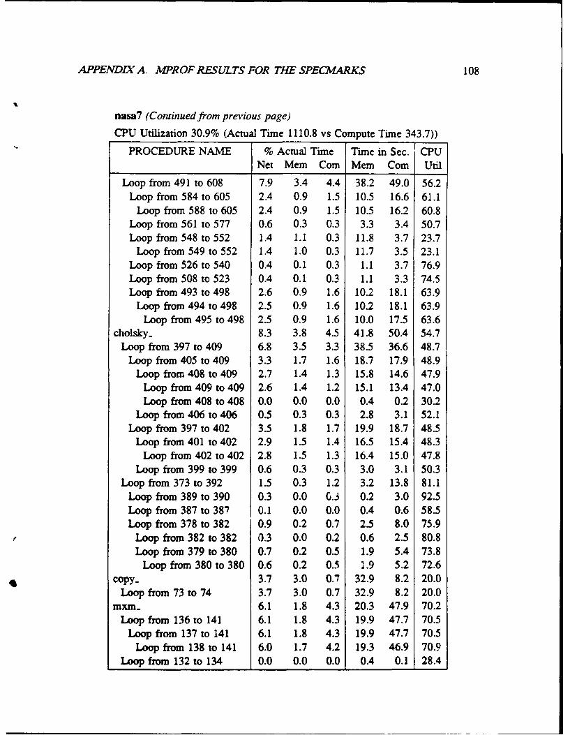
APPENDIX A. MPROF RESULTS FOR THE SPECMARKS 108
nasa7 (Continued from previous page)
CPU Utilization 30.9% (Actual Time 1110.8 vs Compute Time 343.7))
PROCEDURE NAME % Actual Time Time in Sec. ' CPUNet Mem Coin Mem Coin Util
Loop from 491 to 608 7.9 3.4 4.4 38.2 49.0 56.2Loop from 584 to 605 2.4 0.9 1.5 10.5 16.6 61.1
Loop from 588 to 605 2.4 0.9 1.5 10.5 16.2 60.8Loop from 561 to 577 0.6 0.3 0.3 3.3 3.4 50.7Loop from 548 to 552 1.4 1.1 0.3 11.8 3.7 23.7
Loop from 549 to 552 1.4 1.0 0.3 11.7 3.5 23.1Loop from 526 to 540 0.4 0.1 0.3 1.1 3.7 76.9Loop from 508 to 523 0.4 0.1 0.3 1.1 3.3 74.5Loop from 493 to 498 2.6 0.9 1.6 10.2 18.1 63.9
Loop from 494 to 498 2.5 0.9 1.6 10.2 18.1 63.9Loop from 495 to 498 2.5 0.9 1.6 10.0 17.5 63.6
cholsky_ 8.3 3.8 4.5 41.8 50.4 54.7Loop from 397 to 409 6.8 3.5 3.3 38.5 36.6 48.7
Loop from 405 to 409 3.3 1.7 1.6 18.7 17.9 48.9Loop from 408 to 409 2.7 1.4 1.3 15.8 14.6 47.9
Loop from 409 to 409 2.6 1.4 1.2 15.1 13.4 47.0Loop from 408 to 408 0.0 0.0 0.0 0.4 0.2 30.2
Loop from 406 to 406 0.5 0.3 0.3 2.8 3.1 52.1Loop from 397 to 402 3.5 1.8 1.7 19.9 18.7 48.5
Loop from 401 to 402 2.9 1.5 1.4 16.5 15.4 48.3Loop from 402 to 402 2.8 1.5 1.3 16.4 15.0 47.8
Loop from 399 to 399 0.6 0.3 0.3 3.0 3.1 50.3Loop from 373 to 392 1.5 0.3 1.2 3.2 13.8 81.1
Loop from 389 to 390 0.3 0.0 G.3 0.2 3.0 92.5Loop from 387 to 387 0.1 0.0 0.0 0.4 0.6 58.5Loop from 378 to 382 0.9 0.2 0.7 2.5 8.0 75.9
Loop from 382 to 382 0.3 0.0 0.2 0.6 2.5 80.8Loop from 379 to 380 0.7 0.2 0.5 1.9 5.4 73.8
Loop from 380 to 380 0.6 0.2 0.5 1.9 5.2 72.6copy.. 3.7 3.0 0.7 32.9 8.2 20.0
Loop from 73 to 74 3.7 3.0 0.7 32.9 8.2 20.0mxra_ 6.1 1.8 4.3 20.3 47.9 70.2
Loop from 136 to 141 6.1 1.8 4.3 19.9 47.7 70.5Loop from 137 to 141 6.1 1.8 4.3 19.9 47.7 70.5
Loop from 138 to 141 6.0 1.7 4.2 19.3 46.9 70.9Loop from 132 to 134 0.0 0.0 0.0 0.4 0.1 28.4
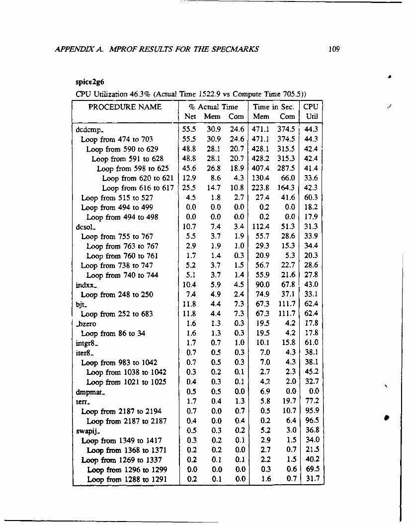
APPENDIX A. MPROF RESULTS FOR THE SPECMARKS 109
at
spice2g6
CPU Utilization 46.3% (Actual Time 1522.9 vs Compute Time 705.5))
PROCEDURE NAME % Actual Time Time in Sec. CPU]Net Mem Corn Mem Com Util
dcdcmp_ 55.5 30.9 24.6 471.1 374.5 44.3Loop from 474 to 703 55.5 30.9 24.6 471.1 374.5 44.3
Loop from 590 to 629 48.8 28.1 20.7 428.1 315.5 42.4Loop from 591 to 628 48.8 28.1 20.7 428.2 315.3 42.4
Loop from 598 to 625 45.6 26.8 18.9 407.4 287.5 41.4Loop from 620 to 621 12.9 8.6 4.3 130.4 66.0 33.6Loop from 616 to 617 25.5 14.7 10.8 223.8 164.3 42.3
Loop from 515 to 527 4.5 1.8 2.7 27.4 41.6 60.3Loop from 494 to 499 0.0 0.0 0.0 0.2 0.0 18.2
Loop from 494 to 498 0.0 0.0 0.0 0.2 0.0 17.9dcsol_ 10.7 7.4 3.4 112.4 51.3 31.3
Loop from 755 to 767 5.5 3.7 1.9 55.7 28.6 33.9Loop from 763 to 767 2.9 1.9 1.0 29.3 15.3 34.4Loop from 760 to 761 1.7 1.4 0.3 20.9 5.3 20.3
Loop from 738 to 747 5.2 3.7 1.5 56.7 22.7 28.6Loop from 740 to 744 5.1 3.7 1.4 55.9 21.6 27.8
indxx_ 10.4 5.9 4.5 90.0 67.8 43.0Loop from 248 to 250 7.4 4.9 2.4 74.9 37.1 33.1
bjt_ 11.8 4.4 7.3 67.3 111.7 62.4Loop from 252 to 683 11.8 4.4 7.3 67.3 111.7 62.4
_bzero 1.6 1.3 0.3 19.5 4.2 17.8Loop from 86 to 34 1.6 1.3 0.3 19.5 4.2 17.8
intgr8_ 1.7 0.7 1.0 10.1 15.8 61.0iter8_ 0.7 0.5 0.3 7.0 4.3 38.1
Loop from 983 to 1042 0.7 0.5 0.3 7.0 4.3 38.1Loop from 1038 to 1042 0.3 0.2 0.1 2.7 2.3 45.2Loop from 1021 to 1025 0.4 0.3 0.1 4.2 2.0 32.7
dmpmat_ 0.5 0.5 0.0 6.9 0.0 0.0terr. 1.7 0.4 1.3 5.8 19.7 77.2
Loop from 2187 to 2194 0.7 0.0 0.7 0.5 10.7 95.9Loop from 2187 to 2187 0.4 0.0 0.4 0.2 6.4 96.5
swapij. 0.5 0.3 0.2 5.2 3.0 36.8Loop from 1349 to 1417 0.3 0.2 0.1 2.9 1.5 34.0
Loop from 1368 to 1371 0.2 0.2 0.0 2.7 0.7 21.5Loop from 1269 to 1337 0.2 0.1 0.1 2.2 1.5 40.2
Loop from 1296 to 1299 0.0 0.0 0.0 0.3 0.6 69.5Loop from 1288 to 1291 0.2 0.1 0.0 1.6 0.7 31.7
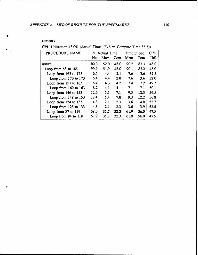
APPENDIX A. MPROF RESULTS FOR THE SPECMARKS 110
tomcatv
CPU Utilization 48.0% (Actual Time 173.5 vs Compute Time 83.3))
PROCEDURE NAME % Actual Time Time in Sec. CPUNet Mem Corn Mem Corn Util
inithx_ 100.0 52.0 48.0 90.2 83.3 48.0Loop from 68 to 185 99.9 51.9 48.0 90.1 83.2 48.0
Loop from 163 to 173 6.5 4.4 2.1 7.6 3.6 32.3Loop from 170 to 173 6.4 4.4 2.0 7.6 3.6 32.0
Loop from 157 to 163 8.4 4.3 4.2 7.4 7.2 49.2Loop from 160 to 163 8.2 4.1 4.1 7.1 7.1 50.1
Loop from 146 to 153 12.6 5.5 7.1 9.5 12.3 56.5Loop from 148 to 153 12.4 5.4 7.0 9.3 12.2 56.8
Loop from 124 to 133 4.3 2.1 2.3 3.6 4.0 52.7Loop from 125 to 133 4.3 2.1 2.3 3.6 3.9 52.4
Loop from 87 to 119 68.0 35.7 32.3 61.9 56.0 47.5Loop from 94 to 118 67.9 35.7 32.3 61.9 56.0 47.5

APPENDIX A. MPROF RESULTS FOR THE SPECMARKS 111
pcl
CPU Utilization 51.1% (Actual Time 73.3 vs Compute Time 37.5))
PROCEDURE NAME % Actual Time Time in Sec. CPUNet Mem Corn Mem Corn Util
malloc 8.5 7.0 1.5 5.1 1.1 18.0Loop from 118 to 186 5.6 4.5 1.1 3.3 0.8 18.9
Loop from 119 to 136 4.0 3.0 1.0 2.2 0.8 25.7new-basic-block 4.0 3.0 1.0 2.2 0.7 24.8
Loop from 473 to 477 3.8 2.8 0.9 2.1 0.7 24.3yyparse 5.3 1.8 3.5 1.3 2.6 66.6
Loop from 44 to 44 5.2 1.7 3.5 1.3 2.6 66.9Loop from 44 to 44 5.1 1.8 3.3 1.3 2.4 64.4
find.reloads 4.8 1.7 3.1 1.3 2.3 64.1Loop from 1114 to 1538 2.2 0.8 1.4 0.6 1.0 63.2
Loop from 1125 to 1518 2.2 0.8 1.4 0.6 1.0 63.0Loop from 1143 to 1427 1.9 0.7 1.2 0.5 0.9 64.1
Loop from 1190 to 1402 1.1 0.3 0.7 0.2 0.5 69.5.bzero 2.4 1.6 0.8 1.2 0.6 32.6
Loop from 86 to 34 2.0 1.5 0.5 1.1 0.4 25.3yylex 3.6 1.5 2.1 1.1 1.5 57.2
Loop from 44 to 44 0.5 0.3 0.1 0.2 0.1 30.7Loop from 44 to 44 0.5 0.3 0.1 0.2 0.1 30.6
gen-rtx 2.6 1.4 1.1 1.1 0.8 44.0Loop from 207 to 232 0.9 0.6 0.4 0.4 0.3 40.7
.write 0.9 0.9 0.0 0.6 0.0 0.0.sbrk 0.8 0.8 0.0 0.6 0.0 0.3make.node 2.0 0.8 1.2 0.6 0.9 61.6-doprnt 1.6 0.7 0.9 0.5 0.7 57.1
Loop from 301 to 991 1.1 0.4 0.8 0.3 0.6 68.4Loop from 301 to 991 1.1 0.4 0.8 0.3 0.6 67.7

APPENDIX A. MPROF RESULTS FOR THE SPECMARKS 112
xlisp
CPU Utilization 76.3% (Actual Time 258.4 vs Compute Time 197.0))
PROCEDURE NAME % Actual Time Time in Sec. CPUNet Mem Com Mem Coin Util
livecar 9.6 5.7 3.9 14.7 10.2 40.9xlsave 12.7 3.8 8.9 9.8 23.1 70.2
Loop from 360 to 364 4.7 0.2 4.5 0.5 11.7 96.2xlobgetvalue 6.4 2.6 3.7 6.8 9.6 58.4mark 7.3 2.3 5.0 5.9 12.9 68.4
Loop from 327 to 389 6.8 2.3 4.5 6.0 11.6 65.8Loop from 362 to 389 3.4 1.7 1.7 4.3 4.4 50.3
sweep 7.1 2.0 5.1 5.1 13.3 72.2Loop from 415 to 445 7.1 2.0 5.1 5.1 13.3 72.2
Loop from 417 to 444 7.1 2.0 5.1 5.1 13.3 72.1newnode 3.7 1.3 2.4 3.5 6.2 64.0xlarg 2.9 1.1 1.8 2.7 4.7 63.3xlevlist 4.1 0.7 3.4 1.9 8.7 81.9
Loop from 204 to 218 2.2 0.2 2.0 0.4 5.2 92.0xleval 8.0 0.5 7.5 1.4 19.3 93.4xlxgetvalue 6.4 0.4 6.0 1.1 15.5 93.2
Loop from 105 to 110 3.7 0.2 3.5 0.5 9.0 95.2Loop from 106 to 110 2.8 0.1 2.7 0.3 7.1 96.3
xlabind 1.1 0.4 0.7 1.0 1.8 63.7consd 0.7 0.3 0.3 0.8 0.9 51.9binary 1.0 0.3 0.7 0.7 1.9 72.6eql 0.6 0.3 0.3 0.7 0.8 55.8cons 0.6 0.3 0.3 0.6 0.9 57.0
r
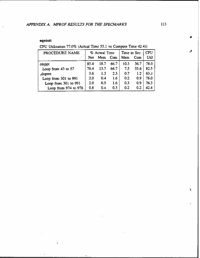
APPENDIX A. MPROF RESULTS FOR THE SPECMARKS 113
eqntott
CPU Utilization 77.0% (Actual Time 55.1 vs Compute Time 42.4))
PROCEDURE NAME % Actual Time Time in Sec. CPUNet Mem Corn Mere Corn Util
cmppt 85.4 18.7 66.7 10.3 36.7 78.0Loop from 43 to 57 78.4 13.7 64.7 7.5 35.6 82.5
..dopmt 3.6 1.3 2.3 0.7 1.2 63.3Loop from 301 to 991 2.0 0.4 1.6 0.2 0.9 78.0
Loop from 301 to 991 2.0 0.5 1.6 0.3 0.9 76.3Loop from 974 to 978 0.8 0.4 0.3 0.2 0.2 42.4

APPENDDI A. MPROF RESULTS FOR THE SPECMARKS 114
doduc
CPU Utilization 77.3% (Actual Tune 95.7 vs Compute Time 74.0))
PROCEDURE NAME % Actual Time Time in Sec. CPUNet Mem Corn Mem Corn Util
subb_ 8.9 4.4 4.5 4.2 4.3 50.4ddeflu_ 6.1 2.3 3.8 2.2 3.6 62.4
Loop from 91 to 255 3.7 1.2 2.5 1.1 2.4 67.8prophy_ 3.1 1.9 1.2 1.9 1.1 37.7
Loop from 52 to 141 2.9 1.8 1.1 1.7 1.1 38.6Loop from 67 to 140 2.3 1.3 0.9 1.3 0.9 41.1
deseco_ 7.1 1.9 5.2 1.8 5.0 73.4Loop from 352 to 407 2.1 0.4 1.7 0.4 1.6 80.0
Loop from 387 to 405 1.2 0.2 1.0 0.2 0.9 80.7Loop from 175 to 193 0.6 0.4 0.3 0.4 0.2 38.7
si. 12.1 1.0 11.1 0.9 10.6 91.8Loop from 16 to 18 8.2 0.6 7.5 0.6 7.2 92.3
pow.p 5.2 0.9 4.3 0.9 4.1 82.1debico_ 1.9 0.9 1.0 0.9 0.9 52.0
Loop from 116 to 125 0.7 0.5 0.2 0.5 0.2 34.1drepvi_ 3.2 0.9 2.3 0.9 2.2 72.1supp_ 7.4 0.7 6.7 0.7 6.4 90.6heat. 1.9 0.7 1.2 0.7 1.2 63.8x2ly2l_ 1.7 0.7 1.0 0.6 1.0 60.6
Loop from 11 to 13 1.6 0.7 0.9 0.6 0.9 58.7dcoera_ 4.1 0.7 3.5 0.6 3.3 84.3paroi_ 1.7 0.6 1.0 0.6 1.0 63.0
Loop from 54 to 70 0.4 0.3 0.1 0.3 0.1 34.7debflu. 1.9 0.6 1.3 0.5 1.3 70.0
Loop from 44 to 185 1.8 0.5 1.3 0.5 1.3 72.1Loop from 74 to 103 0.8 0.2 0.5 0.2 0.5 68.6
4,

APPENDIX A. MPROF RESULTS FOR THE SPECMARKS 115
fpppp
CPU Utilization 79.5% (Actual Time 124.4 vs Compute Time 99.0))
PROCEDURE NAME % Actual Time Time in Sec. CPUNet Mem Corn Mem Corn Util
twldrv_ 59.9 13.1 46.8 16.3 58.2 78.1Loop from 109 to 930 59.9 13.1 46.8 16.3 58.2 78.1
Loop from 112 to 929 59.9 13.1 46.8 16.3 58.2 78.1Loop from 115 to 928 59.9 13.1 46.8 16.3 58.2 78.1
Loop from 118 to 927 59.9 13.1 46.8 16.3 58.2 78.1Loop from 322 to 865 59.0 12.8 46.3 15.9 57.6 78.4
Loop from 333 to 864 59.0 12.7 46.2 15.8 57.5 78.4Loop from 398 to 852 58.0 12.4 45.5 15.5 56.6 78.5
Loop from 417 to 850 57.5 12.2 45.3 15.2 56.3 78.7Loop from 508 to 781 50.1 9.4 40.7 11.7 50.6 81.2
fpppp_ 32.1 3.8 28.4 4.7 35.3 88.2sqrt 2.4 1.2 1.2 1.5 1.5 50.3pow.p 0.7 0.6 0.2 0.7 0.2 23.5
espresso
CPU Utilization 91.8% (Actual Time 38.9 vs Compute Time 35.7))
PROCEDURE NAME % Actual Time Time in Sec. CPUNet Mem Corn Mem Corn Util
malloc 5.4 2.0 3.3 0.8 1.3 62.1massive-count 24.0 1.6 22.5 0.6 8.7 93.5
Loop from 136 to 182 15.7 0.9 14.8 0.4 5.7 94.2Loop from 137 to 182 13.2 0.7 12.6 0.3 4.9 95.0

APPENDIX A. MPROF RESULTS FOR THE SPECMARKS 116
A.1 Discussion of Memory Overheads
K This section analyzes the Mprof profiles for the five SPECmarks which had at least 75%
CPU utilization. The other five SPECmarks with less than 75% CPU utilization are
discussed in Chapter 2. The espresso program has 91.8% CPU utiLization. The Mprof
profile accounts for only part of the memory overhead, with 2.0% of total time spent
in memory overhead in malloc, 1. 6% spent in massive-count, and the remaining
4.4% of execution time divided among procedures that don't execute long enough for
Mprof to accurately time them. Memory overhead in malloc is typically due to cold
start misses (first accesses to data) and hence is difficult to avoid. It is not obvious how
to increase CPU utilization above 92%.
The fpppp program has the next best CPU utilization with only 20.5% of execution
time spent waiting on the memory hierarchy. The memory overhead is spread over many
lines of the program, and Mprof's loop level profile is too crude to isolate the problem
precisely. While the next section describes how Mprof can be enhanced to provide more
detailed information, the conventional wisdom is that good register allocation and careful
instruction scheduling are more significant in fpppp than the 20% memory effect.
The doduc program has 77% CPU utilization, with memory system overhead widely
distributed throughout the code. The Mprof profile reports the procedure with the most
significant memory overhead is subb where memory accounts for 4% of program exe-
cution time. The procedure is called 82380 times and has an ideal compute time of 1725
cycles per call. It uses a fixed data array of 91 double precision constants to evaluate
a polynomial in a single variable H. Virtually all the memory operations in subb are
reads to the an'ay of polynomial coefficients. Given the SGI cache miss penalties, one
can check that the magnitude of the memory overhead measured by Mprof implies the 91
C coefficients are read from memory (not cache) on every call to subb. Thus, to improve
memory system behavior in subb, it would be necessary to identify which memory oper-
ations elsewhere in the program are displacing the elements of the coefficient array from
the cache. This exercise is difficult without full cache simulations, and unlikely to be
beneficial as the other memory accesses are probably unavoidable. In short, Mprof shows
that the memory overhead of subb is difficult to eliminate, and tolerably small. Other

APPEND.I A. MPROF RESULTS FOR THE SPECMARKS 117
overheads are widely distributed throughout doduc with individual procedure overheads
all less than 2%.
The eqntott program spends 23% of its time waiting on the memory hierarchy, with
three quarters of this waiting time concentrated in the cmppt routine. This routine is
called by a quicksort procedure to perform a comparison between two data items for
sorting purposes. To reduce memory overhead, one would certainly need to replace
quicksort with some other sorting algorithm that has better locality. Note, however,
that the CPU utilization of cmppt is already reasonably high (78%), so the potential
for reducing memory overhead is limited, and a less computationally efficient sorting
algorithm may be more expensive overall. It seems best to ignore the memory overhead
and concentrate on simple compute time optimizations like inlining cmppt in quicksort.
The last of the programs with better than 75% CPU is the lisp interpreter xlisp at
76%. About half the memory overhead incurred by the program is in the heap memory
management and garbage collection routines: livecar, mark, sweep, and newnode.
The other half of the overhead is widely distributed over a dozen other routines. The
memory management routines would need to be completely rewritten to change their
cache behavior. Given the limited locality in the heap, this is probably a futile exercise.
Bibliography
[1] M. S. Andersland and T. L. Casavant. Recovering uncorrupted event traces from
corrupted event traces in parallel/distributed computing. In Proceedings of the In-
ternational Conference on Parallel Processing, vol. HI, pages 108-12, Aug. 1991.
[2] T. Anderson and E. Lazowska. Quartz: A tool for tuning parallel program perfor-
mance. In Proceedings of 1990 ACM SIGMETRICS, pages 115-125, May 1990.
[3] Z. Aral and I. Gertner. Non-intrusive and interactive profiling in parasight. In
Proceedings of 1988 ACM/SIGPLAN PPEALS, pages 21-30, 1988.
[4] T. Ball and J. Larus. Optimally profiling and tracing programs. Technical Report
1031, University of Wisconsin-Computer Sciences Dept., 1991.
[5] D. Bernstein, A. Bolmarchich, and K. So. Performance visualization of parallel
programs on a shared memory multiprocessor. In Proceedings of the International
Conference on Parallel Processing, vol. II, pages 1-10, Aug. 1989.
[6] J. Boyle, E. Lusk, et al. Portable Programs for Parallel Processors. Holt, Rinehart,
and Winston, 1987.
[7] H. Burkhart and R. Millen. Performance-measurement tools in a multiprocessor
environment. IEEE Transactions on Computers, 38(5):725-737, 1989.
[8] D. Callahan, K. Kennedy, and A. Porterfield. Analyzing and visualizing performance
of memory hierarchies. In M. Simmons and R. Koskela, editors, Performance
Instrumentation and Visualization, pages 1-26. Addison Wesley, 1990.
118
BIBLJOGRAPHY 119
[9] D. K. Chen. Maxpar: An execution driven simulator for studying parallel systems.
Technical Report CSRD 917, University of Illinois at Urbana-Champaign, 1989.
[10] D. R. Cheriton, H. A. Goosen, and P. D. Boyle. Paradigm: a highly scalable
shared-memory multicomputer architecture. IEEE Computer, 24(2):33-46, 1991.
[11] D. R. Cheriton, H. A. Goosen, and P. Machanick. Restructuring a parallel simulation
to improve cache to behavior in a shared-memory multiprocessor: a first experience.
In Proceedings of the International Symposium on Shared Memory Multiprocessing,
pages 109-118, Apr. 1991.
[12] H. Davis, S. R. Goldschmidt, and J. L. Hennessy. Multiprocessor simulation and
tracing using tango. In Proceedings of the International Conference on Parallel
Processing, vol. II, pages 99-107, Aug. 1991.
[13] H. Davis and J. L. Hennessy. Characterizing the synchronization behavior of par-
allel programs. In Proceedings of ACM/SIGPLAN PPEALS Parallel Programming:
Experience with Applications, Languages and Systems, pages 198-211, 1988.
[14] J. Dongarra, 0. Brewer, J. Kohl, and S. Fineberg. A tool to aid in the design,
implementation, and understanding of matrix algorithms for parallel processors.
Journal of Parallel and Distributed Computing, 9(2):185-202, 1990.
[15] S. J. Eggers and T. E. Jeremiassen. Eliminating false sharing. In Proceedings of
the International Conference on Parallel Processing, vol. I, pages 377-381, Aug.
1991.
[16] K. Gallivan, W. Jalby, A. Malony, and H. Wijshoff. Performance prediction for
parallel numerical algorithms. International Journal of High Speed Computing,
3(l):31-62, 1991.
[17] K. Gallivan, W. Jalby, U. Meier, and A. Sameh. The impact of hierarchical memory
systems on linear algebra algorithm design. International Journal ofSupercomputing
Applications, 2(1), 1988.

BIBLIOGRAPHY 120
[18] D. Gannon, W. Jalby, and K. Gallivan. Strategies for cache and local memory
management by global program transformation. Journal of Parallel and Distributed
Computing, 5(5):587-616, 1988.
[19] D. Gannon, W. Jalby, D. Jablonowski, and Y. Gaur. Faust: an integrated environment
for parallel programming. IEEE Software, 6(4):20-27, 1989.
[20] R. Glenn and D. Pryor. Instrumentation for a Massively Parallel MIMD Application.
Journal of Parallel and Distributed Computing, 12(3):223-236, 1991.
[21] A. Goldberg and J. L. Hennessy. MTOOL: A method for detecting memory bot-
tlenecks. Technical Report WRL TN-17/90, DEC Western Research Laboratory,
1990.
[22] A. Goldberg and J. L. Hennessy. MTOOL: A method for isolating memory bottle-
necks in shared memory multiprocessor programs. In Proceedings of the Interna-
tional Conference on Parallel Processing, vol. II, pages 251-257, Aug. 1991.
[23] A. Goldberg and J. L. Hennessy. Performance debugging shared memory multipro-
cessor programs with mtool. In Proceedings of Supercomputing '91, pages 481-490,
Nov. 1991.
[24] S. Graham, P. Kessler, and M. McKusick. Gprof: A call graph execution profiler.
In Proceedings of ACM/SIGPLAN Symposium on Compiler Construction, pages
120-26, 1982.
[25) M. D. Hill and J. R. Larus. Cache considerations for multiprocessor programmers.Communications of the ACM, 33(8):97-102, 1990.
[26] J. K. Hollingsworth, Irvin R. B., and B. P. Miller. The integration of application and
system based metrics in a parallel program performance tool. In ACM SIGPLAN
Symposium on Principles and Practice of Parallel Programming PPoPP, Apr. 1991.
[27] Donald Knuth. The Art of Computer Programming, Vol 1. Addison-Wesley, 1973.

BIBLIOGRAPHY 121
[28] K. Koh and C. G. Harrison. GETTIMECARD - a basis for parallel program per-
formance tools. Technical Report RC-14993, IBM Research, 1989.
[29] P. Koujianou. Imperfect Competition in International Markets. PhD thesis, Stanford
University Dept. of Economics, May 1992.
[30] A. Kwok and W. Abu-Sufah. Tcedar: A performance evaluation tool for cedar.
Technical Report CSRD 84, University of Illinois at Urbana-Champaign, 1984.
[31] M. S. Lam, E. E. Rothberg, and M. E. Wolf. The cache performance and opti-
mizations of blocked algorithms. In Fourth Conference on Architecural Support for
Programming Languages and Operating Systems, pages 63-74, Apr. 1991.
[32] T. J. LeBlanc, J. M. Mellor-Crummey, and R. J. Fowler. Analyzing parallel program
executions using multiple views. Journal of Parallel and Distributed Computing,
9(2):203-17, 1990.
[33] T. Lehr, D. Black, Z. Segall, and D. Vrsalovic. Mkm: Mach kernel monitor. descrip-
tion, examples and measurements. Technical Report CMU-CS-89-131, Carnegie-
Mellon University-Dept. of Computer Science, 1989.
[34] T. Lehr, Z. Segall, and et. al. Visualizing performance debugging. IEEE Computer,
22(10):38-51, 1989.
[35] D. Lenoski, K. Gharachorloo, J. Laudon, et al. Design of scalable shared-memory
multiprocoessors: The DASH approach. In Proceedings of COMPCON '90, pages
62-67, 1990.
[36] A. Malony. P' rformance Observabiliri. PhD thesis, University of Illinois at Urbana-
Champaign, Oct. 1990.
[37] A. Malony. Event-based performance perturbation. In ACM SIGPLAN Symposium
on Principles and Practice of Parallel Programming PPoPP, 1991.
[38] A. Malony and D. Reed. Models for performance perturbation analysis. In Pro-
ceedings of the ACM/ONR Workshop on Parallel and Distributed Debugging, pages
15-25, May 1991.
BIBLIOGRAPHY 122
[39] M. Martonosi, A. Gupta. and T. Anderson. MemSpy: Analyzing Memory System
Bottlenecks in Programs. In Proceedings of ACM SIGMETRICS, Jun. 1992.
[40] J. D. McDonald and D. Baganoff. Vectorization of a particle simulation method for
hypersonic rarified flow. In Proceedings of AIAA Thermodynamics, Plasmadynamics
and Lasers Conference, Jun. 1988.
[41] S. McFarling. Procedure merging with instruction caches. In SIGPLAN Conference
on Programming Language Design and Implementation, pages 71-91, Jun. 1991.
[42] B. Miller, et al. IPS-2: The second generation of a parallel program measurement
system. IEEE Transactions on Parallel and Distributed Systems, 1(2):206-217,
1990.
[43] A. Mink, R. J. Carpenter, G. G. Nacht, and J. W. Roberts. Multiprocessor
performance-measurement instrumentation. IEEE Computer, 23(9):63-75, 1990.
[44] MIPS Computer Systems, Inc., Sunnyvale, CA. Language Programmer's Guide,
1986.
[45] P. P. Mishra, 0. Gudmundsson, and A. K. Agrawala. Exmon: a tool for resource
monitoring of programs. Tech'nical Report TR-2688, University of Maryland-Dept.
of Computer Science, 1991.
[46] W. Morris. Ccg: A prototype coagulating code generator. In SIGPLAN Conference
on Programming Language Design and Implementation, pages 45-58, Jun. 1991.
[47] T. Mowry and A. Gupta. Tolerating latency through software-controlled prefetching
in scalable shared-memory multiprocessors. Journal of Parallel and Distributed
Computing, 12(3):86-106, 1991.
[48] K. M. Nichols. Performance tools. IEEE Software, 7(3):21-30, 1990.
[49] K. Pettis and R. Hanson. Profile guided code positioning. In SIGPLAN Conference
on Programming Language Design and Implementation, pages 16-27, Jun. 1990.
BIBLIOGRAPHY" 123
[50] M. H. Reilly. A Performance Monitor for Parallel Programs. Academic Press,
1990.3
[51] E. Rothberg and A. Gupta. Techniques for improving the performance of sparse ma-
trix factorization on multiprocessor workstations. In Proceedings of Supercomputing
'90, pages 232-41, Nov. 1990.
[52] D. C. Rudolph and D. A. Reed. CRYSTAL: Intel ipscl2 operating system instru-
mentation. In Proceedings of the Fourth Conference on Hypercubes, Computers
and Applications, Mar. 1989.
[53) A. D. Samples. Profile-Driven Compilation. PhD thesis, University of California at
Berkeley, Apr. 1991.
[54] V. Sarkar. Determining average program execution times and their variance. In
Sigplan Conference on Programming Language Design and Implementation, pages
298-312, 1989.
[55] Zary Segall and Larry Rudolph. PIE: A programming and instrumentation environ-
ment for parallel processing. IEEE Software, 2(11):22-37, 1985.
[56] M. Simmons and R. Koskela, editors. Instrumentation for Future Parallel Comput-
ing Systems. Addiso ,-Wesley, 1989.
[57] M. Simmons and R. Koskela, editors. Performance Instrumentation and Visualiza-
tion. Addison-Wesley, 1990.
[58] J. P. Singh, W-D. Weber, and A. Gupta. Splash: Stanford parallel applications
for shared-memory. Technical Report CSL-TR-91-469, Stanford Computer Systems
Laboratory, 1991.
[59] Spec benchmark suite release 1.0, Oct. 1989. p
[60] T. Sterling, A. Musciano, B. Donald, and R. Osborne. Multiprocessor performance
measurement using embedded instrumentation. In Proceedings of the International
Conference on Parallel Processing, vol. II, pages 156-165, Aug. 1988.

BIBLUOGRAPHY 124
[61] S. S. Thakkar. Performance of parallel applications on a shared-memory multiproces-
sor system. In M. Simmons and R. Koskela, editors, Performance Instrumentation
and Visualization, pages 235-258. Addison Wesley, 1990.
[62] J. Torrellas, M. Lam, and J. L. Hennessy. Shared data placement optimizations
to reduce multiprocessor cache miss rates. In Proceedings of the International
Conference on Parallel Processing, vol. II, pages 266-270, Aug. 1990.
[63] D. Wall. Predicting program behaviour using real or estimated profiles. In SIGPLAN
Conference on Programming Language Design and Implementation, pages 59-70,
Jun. 1991.
9


