Multiple imputation for model checking:
completed-data plots with missing and latent data∗
Andrew Gelman† Iven Van Mechelen‡ Geert Verbeke§
Daniel F. Heitjan¶ Michel Meulders‖
April 17, 2004
Abstract
In problems with missing or latent data, a standard approach is to first imputethe unobserved data, then perform all statistical analyses on the completed data set—corresponding to the observed data and imputed unobserved data—using standardprocedures for complete-data inference. Here, we extend this approach to model check-ing by demonstrating the advantages of the use of completed-data model diagnosticson imputed completed data sets. The approach is set in the theoretical framework ofBayesian posterior predictive checks (but, as with missing-data imputation, our meth-ods of missing-data model checking can also be interpreted as “predictive inference” ina non-Bayesian context). We consider graphical diagnostics within this framework.
Advantages of the completed-data approach include: (1) One can often check modelfit in terms of quantities that are of key substantive interest in a natural way, whichis not always possible using observed data alone. (2) In problems with missing data,checks may be devised that do not require to model the missingness or inclusion mech-anism; the latter is useful for the analysis of ignorable but unknown data collectionmechanisms, such as are often assumed in the analysis of sample surveys and observa-tional studies. (3) In many problems with latent data, it is possible to check qualitativefeatures of the model (for example, independence of two variables) that can be nat-urally formalized with the help of the latent data. We illustrate with several appliedexamples.
Keywords: Bayesian model checking, exploratory data analysis, multiple imputa-tion, nonresponse, posterior predictive checks, realized discrepancies, residuals
∗To appear in Biometrics. We thank Phillip N. Price and several reviewers for helpful comments. Thiswork was supported in part by fellowship F/96/9 and Research Grant OT/96/10 of the Research Councilof Katholieke Universiteit Leuven, grant grant IAP P5/24 of the Belgian Federal Government, and grantsSBR-9708424, SES-9987748, SES-0318115, and Young Investigator Award DMS-9796129 of the U.S. NationalScience Foundation.
†Department of Statistics, Columbia University, New York, USA, [email protected],
http://www.stat.columbia.edu/∼gelman/‡Psychology Department, Katholieke Universiteit Leuven, Belgium§Biostatistical Centre, Katholieke Universiteit Leuven, Belgium¶Division of Biostatistics, University of Pennsylvania, Philadelphia, USA‖Psychology Department, Katholieke Universiteit Leuven, Belgium
1

1 Introduction
1.1 Difficulties of model checking with missing and latent data
The fundamental approach of goodness-of-fit testing is to display or summarize the observed
data, and compare this to what might have been expected under the model. If there are
systematic discrepancies between the data summaries and their reference distribution under
the assumed model, this implies a misfit of the model to the data. Model checks include
analytical methods such as χ2 and likelihood ratio tests, and graphical methods such as
residual and quantile plots. In missing and latent data settings, two complications arise that
can in practice often lead to models being checked in only a cursory fashion if at all.
The first complication comes because in missing-data situations the reference distribution
of a data summary, whether analytical or graphical, is implicitly determined by the data
that could have been seen under the model. As a result, comparing the data to what could
have been observed requires a model for the missing-data mechanism—in order to obtain a
reference distribution for which data points are observed—as well as a model for the data
themselves. Modeling the process that generated the missing data can be difficult, and
any requirement that this be done will drastically reduce the practicality of model checking
procedures. As a result, model checking is generally applied either to complete-data segments
of the problem or only approximately.
The second complication arises with latent data (defined broadly to include, for example,
group-level parameters in hierarchical models). Even if there is a full model for the observa-
tion process (and, hence, it is not a problem to simulate replications of the observed data),
the latent data may be of scientific interest. As such, we may wish to construct tests using
these latent categories or variables. As an example, one may think of regression diagnostics
in hierarchical models involving residuals calculated on the basis of group-level parameters
(that are considered as latent data). Unlike standard residuals that are difficult to interpret
2

for hierarchical models (see Hodges, 1988), those based on latent data are independent.
The characterization of unobserved data as “missing” or “latent” is somewhat arbitrary;
as is well known in the context of EM and similar computational algorithms, latent and
missing data have the same inferential standing as unknown quantities with a joint distribu-
tion under a probability model. For the purpose of this paper, we distinguish based on the
interpretation of the completed dataset: missing data have the same structure as observed
data whereas latent data are structurally different. For example, Section 4.2 describes a
situation in which children’s ages are reported rounded to the nearest one, six, or twelve
months (see the top graph in Figure 6). We consider the children’s true ages as latent data,
in that if we were given the completed dataset (all the true ages and all the reported ages),
then we would wish to distinguish between the true and reported ages—they play different
roles in the model. In fact, in this example, the type of rounding (whether to one, six, or
twelve months) is another latent variable. How could missing data arise in this context?
If some of the children in the study were missing some recorded covariates, or if age were
not even reported for some children, these would be missing data—because, once these data
were imputed, they would be structurally indistinguishable from the observed data.
1.2 Predictive checks with unobserved data
In this paper, we propose to resolve difficulties of model checking in missing and latent
data settings using the framework of Bayesian posterior predictive checks (Rubin, 1984,
Gelman, Meng, and Stern, 1996). The general idea of predictive assessment is to evaluate
any model based on its predictions given currently-available data (Dawid, 1984). Predictive
criteria can be used as a formal approach for evaluation and selection of models (Geisser and
Eddy, 1979, Seillier-Moiseiwitsch, Sweeting, and Dawid, 1992). Here we focus on graphical
and exploratory comparisons (as in Buja et al., 1988, Buja, Cook, and Swayne, 1999, and
Gelman, 2004), in addition to numerical summaries based on test statistics.
3

Gelman, Meng, and Stern (1996) define posterior predictive checks as comparisons of
observed data yobs to replicated data sets yrep
obs that have been simulated from the posterior
predictive distribution of the model with parameters θ. In this paper we extend posterior
predictive checking within the context of missing or latent data by including unobserved
data in the model checks. Model checking then will be applied to completed data which will
typically require multiple imputations of the unobserved data.
The approach of including unobserved data in model checks will be shown to yield vari-
ous advantages. The situation is similar to that of the EM algorithm (Dempster, Laird, and
Rubin, 1977), data augmentation (Tanner and Wong, 1987), and multiple imputation (Ru-
bin, 1987, 1996). The EM and data augmentation algorithms take advantage of explicitly
acknowledging unobserved data in finding posterior modes and simulation draws. The mul-
tiple imputation approach similarly accounts for uncertainties in missing data for Bayesian
inference. The approach proposed in the present paper then completes this idea for model
checking. In general, a key advantage of completed-data model checks is that they can be
directly understandable in ways that observed data checks are not, allowing, for example,
graphical model checks (analogous to residual plots) that are interpretable without need for
formal computation of reference distributions. We shall illustrate this with several instances
of missing and latent data problems from a wide range of application areas, with various
statistical models, and a variety of graphical displays.
Despite the simplicity of the approach, we have seen it only rarely in the statistical
literature (with exceptions including the analysis of realized residuals in linear models and
censored-data models, Chaloner and Brant, 1998, and Chaloner, 1991; and latent continuous
responses in discrete-data regressions, Albert and Chib, 1995). We attribute this to an
incomplete conceptual foundation. We hope that this paper, by placing completed-data
diagnostics in a general framework (in which observed-data test statistics are a special case),
4

and illustrating in a variety of applications, will motivate their further use.
This paper is organized as follows. Section 2 defines the basic notation and ideas under-
lying our recommended approach, first for missing and then for latent data. Sections 3 and 4
present several examples from applied work by ourselves and others, and Section 5 discusses
some of the lessons we have learned from these applied examples.
2 Notation, underlying ideas, and implementation
We set up our completed-data model checking using the theoretical framework of Little
and Rubin (1987) and Gelman et al. (2003, chapter 7) for Bayesian inference with missing
data. The two relevant tasks are defining the predictive distribution for replicated data,
and choosing the completed-data summaries to display. We discuss the theoretical issues in
detail in Section 2.1 for the case of missing data and then in Section 2.2 briefly consider the
latent data setting. We present our approach in algorithmic form in Section 2.3.
2.1 Missing data
2.1.1 Bayesian notation using inclusion indicators
We use the term missing data for potentially observed data that, unintentionally or by design,
have been left unobserved. Consider observed data yobs and missing data ymis, which together
form a “completed” data set ycom = (yobs, ymis). If y were fully observed, we would perform
inference for the parameter vector θ defined by the data model p(y|θ) and possibly a prior
distribution p(θ). Instead, we must condition on the available information: the observed
data yobs and the inclusion indicator vector I, which describes which units of y are observed
and which are not. (For simple scenarios of missingness, we would label Ii = 1 for observed
data i and 0 for missing data. More generally, I could have more than two possible values in
settings with partially-informative missing-data patterns such as censoring, truncation, and
rounding.) The model is completed by a probabilistic “inclusion model,” p(I|ycom, φ), with
5

a prior distribution p(φ|θ) on the parameters φ of the inclusion model.
Bayesian analysis then works with the joint posterior distribution p(θ, φ, ymis|yobs, I) ∝
p(θ)p(φ|θ)p(ycom|θ)p(I|ycom, φ). It is necessary to formally include I in the model because, in
general, the pattern of which data are observed and which are unobserved can be informative
about the parameters of interest in the model. In addition, all these probability distributions
are implicitly conditional on any fully-observed covariates.
An important special case occurs if p(θ, ymis|yobs, I) = p(θ, ymis|yobs) ∝ p(θ)p(ycom|θ), in
which case the inclusion model is ignorable (Rubin, 1976). A key issue in using ignorable mod-
els is that they do not require a model p(I|ycom, φ) or a functional form for p(φ|θ). Two jointly
sufficient conditions for ignorability are “missingness at random”—that the probability of
the missing data pattern depends only on observed data—and “distinct parameters”—that φ
and θ are independent in their prior distribution. In practice, most statistical analyses with
missing data either assume ignorability (after including enough covariates in the model so
that the assumption is reasonable; for example, including demographic variables in a sample
survey and making the assumption that nonresponse depends only on these covariates) or
set up specific nonignorable models. As we shall discuss in Section 2.1.3 and in the example
in Section 3.1, under an ignorable model one can simulate replications of the completed data
ycom without ever having to simulate or model the missing-data mechanism.
2.1.2 Posterior predictive replications in case of missing data
Replicating the complete data is relatively simple, requiring knowledge only of the complete-
data model and parameters, whereas replicating the observed data also requires a model for
the missingness mechanism. Thus, from the standpoint of replications, observed datasets—
which are characterized by (ycom, I)—are more complicated than completed datasets ycom.
To simulate replicated datasets for model checking, one can start with the observed data
and observed inclusion pattern (yobs, I), then estimate the parameter vector θ simultaneously
6

with the missing data ymis—this is the data augmentation paradigm of Dempster, Laird, and
Rubin (1977) and Tanner and Wong (1987). In simulation-based inference, the result is
a set of “multiple imputations” l = 1, . . . , L of the completed data ylcom along with the
corresponding draws of the parameters (θl, φl). The completed data sets can be compared
to their expected distribution under the model, or to properties of the reference distribution
such as independence, zero mean, or smoothness.
In general, a replicated experiment can lead to a different missing data pattern, and so
the reference distribution for yobs must be determined from the reference distribution of ycom
along with that of the inclusion pattern I.
2.1.3 Test variables in the presence of missing data
In predictive model checking, test variables can be thought of as data displays or summaries,
and a key issue is how to construct graphical summaries to reveal important (and often
unanticipated) model flaws. This is the problem of exploratory data analysis (Tukey, 1977),
here in a modeling context. The best way to understand these choices is to look at practical
examples, as we do in Sections 3 and 4 of this paper. We set up general notation here.
With missing-data, the most general form of a test variable is T (ycom, I, θ, φ), the corre-
sponding posterior predictive replication being T (yrepcom, Irep, θ, φ). Since yobs is a deterministic
function of ycom and I, this formulation includes observed-data tests as a special case. In
general, we imagine replicating ycom and possibly replicating I, but the latter only if the test
quantity depends on the pattern of missing data. As we discuss here and in the examples,
it often makes sense to choose a test variable that depends only on ycom and not on I at all.
Although test variables of the form T (yobs) are easier to compute for any given data
set, we would like to consider test variables of the form T (ycom), for three reasons. First,
the substantive interest typically lies in the complete-data model (what we would do if we
observed all the data), so a test variable based on the completed data should be easier
7

to understand substantively. This is important, considering that “practical significance” is
as important as “statistical significance” in model checking. Second, as noted at the end
of the previous section, the posterior predictive distribution for yrepcom depends only on the
complete-data model (and, of course, the posterior distribution for θ), whereas the posterior
predictive distribution for yrep
obs can also depend on the distribution for the inclusion variable
(because the observed units need not be the same in the observed and replicated data). As
a result, test statistics of the form T (ycom) can be checked using fewer assumptions than are
required to test T (yobs). This is particularly important when using ignorable models such as
are often assumed in the analysis of observational studies (see Gelman et al., 2003, Section
7.7). Third, in many cases the reference distribution of the replicated test variable, T (yrepcom),
has a particularly simple form, often involving independence among variables. As a result,
the model can be checked informally using just the simulated realized values, T (ycom), with
an implicit comparison to a known reference distribution.
2.2 Latent data
Latent data can be defined as structurally unobserved variables that play a key role in
the model for the observed data. Consider observed data yobs that are modeled in terms
of latent data ylat, with “completed” data set (yobs, ylat). Latent data problems may be
considered a special case of the general missing data case, characterized by a structurally
modeled inclusion variable I. Bayesian analysis then uses the joint posterior distribution
p(θ, ylat|yobs) ∝ p(θ)p(ylat|θ)p(yobs|ylat, θ).
In the latent data context, I is structurally fixed, and so there are no inclusion-model
parameters φ. Hence, we then have two main possibilities to define the posterior predictive
replications: (a) keeping ylat fixed and varying yobs (that is, setting yrep
lat = ylat and drawing
yrep
obs from p(yobs|ylat, θ), (b) varying both ylat and yobs (that is, drawing (yrep
lat , yrep
obs) from
p(ylat, yobs|θ) = p(ylat|θ)p(yobs|ylat, θ)).
8

In the latent data context the most general form of a test summary is T (yobs, ylat, θ),
the corresponding posterior predictive replication being T (yrep
obs, yrep
lat , θ). This formulation
includes observed-data test summaries as a special case. In general, we recommend examining
test summaries that check in a natural way key features of the model under consideration.
In many latent data models such summaries will depend on ylat as well as yobs.
Many datasets fit with latent-data models also have missing data. One can then put
the inclusion indicators I into the model and proceed as in Section 2.1, with the additional
feature that latent data are present. Test variables can be defined from the completed
observable data ycom, which includes the imputations of the missing and latent data.
2.3 Implementation
The most general implementation of completed-data model checks proceeds in three steps:
1. Perform inference jointly for the parameters θ (and, if necessary, φ) and the missing
and latent data ymis, ylat, thus obtaining a set of L imputed datasets ycom. Inference
for the model parameters can be represented by a point estimate or, more generally,
by L draws from the posterior distribution.
2. Construct a test variable—in the context of this paper, often a graph—that is a function
of the completed data, ycom and possibly the inclusion indicators I and the parameters
θ. The L imputations induce L possibilities for the test variable, and these can be
displayed as multiple imputations (as in the second or third row of Figure 6).
3. Construct the reference distribution of the test variable, which can be done analytically
(as with some χ2 tests), or using the complete-data model given a point estimate of the
parameters, or given posterior simulations of the parameters, or using other approaches
such as cross-validation or bootstrapping to summarize inferential uncertainties. In any
case, the result is a distribution, or a set of simulated replications, of the test variable
9

assuming the fitted model. Depending on the details of the problem, the replications
can be displayed graphically, for example as in the overlain lines in Figures 2 and 3.
For observed data model checks—or more generally, for any test variables that depend on I
as well as ycom—the third step requires replication of the inclusion indicators as well as the
complete data, as discussed in Section 2.1.3.
In practice, it is often convenient to simplify step 2 above. Data sets typically have
internal replication, and often a single random imputation conveys the look of a graphical
test variable, without the need for displaying several random draws. The bottom row of
plots in Figure 4, for example, displays a single completed dataset. For simplicity we often
work with a single imputation if the data have enough structure. A related strategy is to
create the diagnostic plot several times and, if the multiply-imputed completed datasets look
similar, to display just one of them. When summarizing with a numerical test statistic, one
can use the entire distribution to compute p-values, as we illustrate in Section 4.1.
We can often simplify step 3—the computation and display of the reference distribution—
by comparing the graphical test variable to an implicit reference distribution. For example,
residual plots are compared to the null hypothesis of zero mean and independence. (In
a latent-data posterior predictive framework, unlike with point estimation, residuals are
independent in their reference distribution.) We shall illustrate less structured implicit com-
parisons in Figures 4 and 6.
3 Applications with missing data
3.1 Randomized experiments with an ignorable dropout model
A common problem in studies of persons or animals is that subjects drop out in the middle of
the experiment, creating a problem of missing data. After imputation, we can use completed-
data methods to check model fit, as we illustrate here.
10

Verbeke and Lesaffre (1999) analyzed longitudinal data from a randomized experiment,
the aim of which was to study the effect of inhibiting testosterone production on the cran-
iofacial growth of male Wistar rats. A total of 50 rats were randomly assigned to either a
control group or one of the two treatment groups where treatment consisted of a low or high
dose of the drug Decapeptyl, which is an inhibitor for testosterone production in rats. The
treatment started at the age of 45 days, and measurements were taken at 50 days and every
10 days thereafter. The responses of interest are distances (in pixels) between well-defined
points on x-ray pictures of the skull of each rat, taken after the rat has been anaesthetised.
See Verdonck et al. (1998) for a detailed description of the experiment.
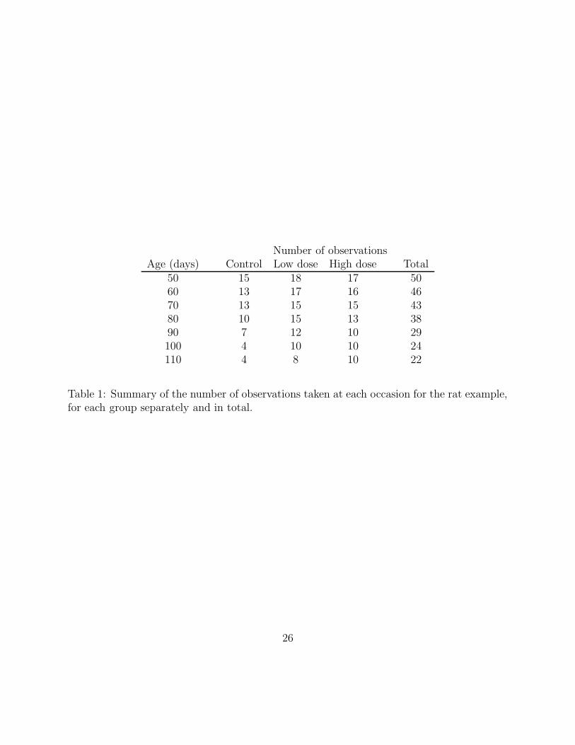
For the purpose of this paper, we consider one of the measurements that can be used
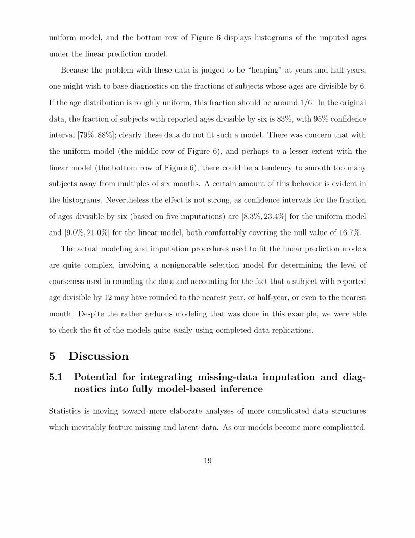
to characterize the height of the skull. The individual profiles are shown in Figure 1 and
show a high degree of dropout. Indeed, many rats do not survive anaesthesia and therefore
drop out before the end of the experiment. Table 1 shows the number of rats observed at
each occasion. Of the 50 rats randomized at the start of the experiment, only 22 survived
all seven measurements. Verbeke and Lesaffre (1999) studied the effect of the dropout on
the efficiency of the final testing procedures, and derived alternative designs with less risk of
huge losses of efficiency when dropout would occur. They modeled the jth measurement yij
for the ith rat, j = 1, . . . , ni, i = 1, . . . , N , as
yij =
β0 + β1tij + bi + εij, if low doseβ0 + β2tij + bi + εij, if high doseβ0 + β3tij + bi + εij, if control dose,
(1)
where the transformation tij = log(1 + (Ageij − 45)/10)) is used to linearize the subject-
specific profiles. The parameter β0 then represents the average response at the time of
treatment, and β1, β2, and β3 represent the average slopes for the low dose, high dose, and
control groups. The assumption of a common average intercept is justified by the random-
ization of the rats. For each subject i, the parameter bi fits the deviation of its intercept
from the average value in the population, and the εij’s denote the residual components; it is
11

assumed that they all are independently and normally distributed with mean 0 and standard
deviations σb and σε respectively.
Inspection of Figure 1 suggests a specific model violation: in the high-dose condition, the
residual variance seems to be smaller than in the two other conditions, at least before age
75 days. Such a result could be interesting in understanding the effects of the treatment.
However, it is hard to interpret this graph because, even under an ignorable model, dropout
can depend on previous measurements. For example, a lack of extreme measurements at
high time values could be explained by dropout rather than by underlying data.
The assumption of ignorability can, by definition, never be formally checked without
making strong assumptions about possible associations between dropout and the missing
outcomes, and it is important to study the sensitivity of the conclusions to the underlying
assumptions. This data set has previously been extensively analyzed (see Verbeke et al.,
2001), and based on conversations with the clinicians involved in this experiment, there
seems to be no clinical evidence that missingness might depend on unobserved outcomes.
In this example we can safely assume ignorability of the inclusion mechanism; we therefore
use (1) to impute the missing data (based on mixed-model estimates for the parameters bi).
Next we calculate, for each age, the standard deviation across rats of the ycom-values. This
standard deviation captures both the between-rat variance in intercept bi and the residual
variance σε. (Because we calculate the test summary separately for each simulation draw, this
standard deviation is not inflated by estimation uncertainty in the posterior distribution.)
The results of a single randomly imputed completed dataset—the observed data supple-
mented with a random draw of the missing data from the posterior distribution—appear in
Figure 2, along with the standard deviations of 20 replicated data sets (again based on the
mixed-model estimates). This figure supports the impression that the residual variance in
the high-dose condition is somewhat smaller than assumed under the model whereas the re-
12

verse seems to hold for the low-dose condition. The pattern is suggestive but not statistically
significant, in that the replications show that such a pattern is possible under the model.
This finding inspired us to try out a model expansion with condition-dependent residual
variances σε1 , σε2 and σε3. Such a model expansion can be justified on substantive grounds
as it formalizes dose-dependent irregularities in growth speed. A likelihood ratio statistic
revealed that the expanded model tends to be preferable over the original model (1), LR=5.4,
df=2, p=0.067, whereas for the expanded model AIC=943.0 and for model (1) AIC=944.4.
Figure 3 checks the expanded model for the replication of the 20 datasets as well as for the
imputation of the missing outcomes. When compared to Figure 2, the completed standard
deviation lines are clearly more in the center of the reference distribution of replicated data,
especially towards the end of the study (where most of the missingness occurs). Note also
the much smaller completed standard deviation at 60 days in the control group (compared to
Figure 2), even though an imputation is needed at that time point for two rats only. However,
one of these rats had an exceptionally small initial value (at 50 days). The imputation is
now based on a smaller residual variance, hence a larger within-subject correlation, implying
that the imputed value at age 60 days for this rat will tend to be smaller as well. Finally,
the control group is also the smallest, containing only 15 rats.
These results show that our graphical approach to checking fit is useful in that it helps
in finding out relevant directions for specifying alternative models. If desired, candidate
models that are generated in this way can be compared using numerical criteria (e.g., AIC).
In the rat example, in this way, a potentially meaningful model improvement was obtained,
suggested by the results of the graphical check.
3.2 Clinical trials with nonignorable dropout
The previous example illustrated the common setting in which missing data are imputed
using an ignorable model. In other settings, however, dropout is affected by outcomes under
13

study that have not been fully recorded, and so it often makes sense to use nonignorable
models (for example, in a study of pain relief drugs, a subject may drop out if he or she
continues to feel pain). As a result, the analysis cannot simply be done on the observed data
alone (Diggle and Kenward, 1994). Methods based on Bayesian modeling of dropouts can
be thought of as multiple imputation approaches in which (a) the measurements that would
have occurred are imputed, and then (b) a completed-data analysis is performed. A key
intermediate stage here is the completed data set, which we can plot to see if any strange
patterns appear. We illustrate with an example from Sheiner, Beal, and Dunne (1997).
The top row of Figure 4 shows the distribution of recorded pain measurements over time
for patients who were randomly assigned to be given one of three doses of a new pain relief
drug immediately following a dental operation. In this top row of plots, the width of the bar
at each time represents the proportion of participants still in the trial. Patients were allowed
to drop out at any time by requesting to be switched to a pain reliever that is known to be
effective. The data show heavy dropout, expecially among the controls. In addition, there
seems to be a pattern of decreasing pain over time at all doses—but it is not clear how this
is affected by the dropout process.
Sheiner, Beal, and Dunne (1997) fit to these data a model with three parts. Internally
for each subject is a pharmacokinetic differential equation model of the time course of the
concentration of the drug in different compartments of the body. This model implicitly
includes an impulse-response function of internal concentrations to administered doses of
the drug. At the next level, the pain relief data were fit by an ordered multinomial logistic
model with probabilities determined by a nonlinear function of the internal concentration of
the drug. Finally, missingness was modeled nonignorably, with the probability of dropping
out depending on the pain level at the time (which is unobserved under dropout).
Once this model has been fit to data, it can be used to make predictions under alternative
14

input conditions, as demonstrated by Sheiner, Beal, and Dunne (1997), who determine a
more effective dosing regimen that is estimated to give a consistently high level of pain relief
with a low total dose. In addition, the model yields estimated uncertainty distributions for
the underlying full time series of pain scores that would have occurred for each patient in the
absence of dropout. We show here (following Gelman and Bois, 1997) how these imputed
pain scores can be used to summarize the estimated underlying patterns in the data.
The bottom row of Figure 4 shows graphs similar to the top row, but of the completed
dataset with imputations for the dropouts. (Here, a simple deterministic scheme was used for
the imputations, but the method could be used with multiple imputations, leading to several
sets of graphs corresponding to the different imputations.) For all doses, the completed data
show immediate pain relief followed by some increasing pain. These plots show the dose-
response relation far more clearly than did the observed-data plots in the top row.
Plotting the completed dataset is interesting here even if it does not reveal model flaws:
the completed dataset is much easier to understand and interpret than the plot of observed
data alone, and substantive hypotheses are more directly interpretable in terms of the com-
pleted data. These plots can be seen as a model check, not compared to a posterior predictive
distribution but rather to whatever substantive knowledge is available about pain relief.
4 Applications with latent data
4.1 Latent psychiatric classifications
Psychiatric symptom judgments of patients by psychiatrists and clinical psychologists may
be based on implicit classifications of the patients by the clinicians in some implicit syndrome
taxonomy that is shared by the clinicians (Van Mechelen and De Boeck, 1989). According
to a clinician, a symptom then will be present in some patient if there is at least one implicit
syndrome that applies to that patient and that implies the symptom in question. Maris,
15

De Boeck, and Van Mechelen (1996) have formalized this idea in a model that includes
probabilistic links between symptoms and latent syndromes on the one hand, and between
patients and latent syndromes on the other hand. In particular, let (yobs)ijk equal 1 if patient
i has symptom j according to clinician k, and (yobs)ijk equal 0 otherwise. The assumed model
then implies latent variables for the patients (ylat,p)ijkl and latent variables for the symptoms
(ylat,s)ijkl, each pertaining to l = 1, . . . , L latent syndromes:
(ylat,p)ijkl =
1 if, when patient i is judged on symptom j by clinician k,this patient is considered to suffer from latent syndrome l
0 otherwise
(ylat,s)ijkl =
1 if, when patient i is judged on symptom j by clinician k,this symptom is considered to be implied by latent syndrome l
0 otherwise
The model further assumes that:
(ylat,p)ijkl ∼ Bern(θp,il)
(ylat,s)ijkl ∼ Bern(θs,jl),
all latent variables being independent. As stated above, clinician k will then judge symptom
j to be present in patient i if there is at least one syndrome l for which (a) patient i is judged
by clinician k to suffer from it, and (b) symptom j is judged by clinician k to be implied by
it. Stated formally:
(yobs)ijk = 1 if there exists an l for which (ylat,p)ijkl = 1 and (ylat,s)ijkl = 1.
When fitting the model to symptom judgments of patients by several clinicians, the model as-
sumptions could be violated if there are systematic differences between clinicians in the links
between symptoms and latent syndromes. Natural test variables to check this assumption
can be defined making use of the latent Bernoulli variables ylat,s.
We illustrate with data from Van Mechelen and De Boeck (1990) on 23 psychiatric
symptom judgments for 30 patients by 15 clinicians. As test variables we calculate, for each
16

symptom j and for each latent syndrome l, the variance across clinicians of the summed
realizations of the corresponding symptom-syndrome link variable:
Tjl =1
K
∑
k
[
∑
i
(ylat,s)ijkl
]2
−
[
1
K
∑
k
∑
i
(ylat,s)ijkl
]2
.
We further summarize the fit for each syndrome and symptom by posterior predictive p-
values; for any test variable Tjl(ylat,s), the p-value is Pr(Tjl(yrep
lat,s) > Tjl(ylat,s)), and can be
computed using the set of M multiple imputations of the parameters and completed data
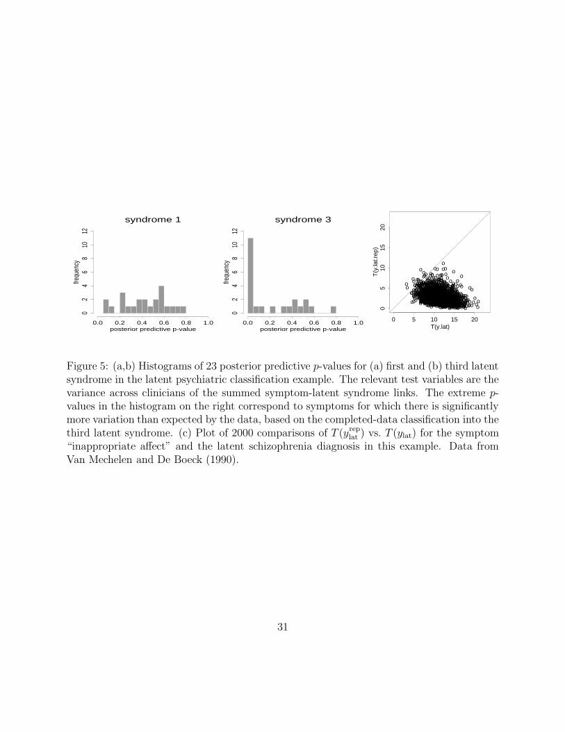
set (Meng, 1994b, Gelman, Meng, and Stern, 1996). Figure 5a shows the histogram of the
posterior predictive p-values for the between-clinician variance for the link between the first
syndrome and each of 23 symptoms, and Figure 5b shows the corresponding histogram for the
third latent syndrome (which could be identified as an implicit schizophrenia syndrome). For
the third, unlike for the first, latent syndrome, the variation in several symptom-syndrome
links across clinicians is greater in the data than assumed under the model. This can be
further clarified by plots such as Figure 5c, which shows a plot of 2000 pairwise comparisons of
Tjl(yrep
lat,s) and Tjl(ylat,s) for the symptom “inappropriate affect” and the latent schizophrenia
diagnosis. This example illustrates how model checks can be formed using latent data only.
4.2 Rounded and heaped data
We next illustrate with an example of imputed continuous latent data. Heitjan and Rubin
(1990) analyzed a survey of children’s health in Africa in which the exact ages of the chil-
dren are not known—only “reported ages” given by the parents were available, along with
anthropometric data including height and weight. The original purpose of the survey was
to combine height and weight with recorded age to produce tables classifying the children
by nutritional status: being thin for one’s height suggests current malnutrition, and being
short for one’s age suggests a history of malnutrition. Standard curves for these variables are
based on data from the U.S., where children’s ages are typically known with great accuracy.
17

The top histogram in Figure 6 shows the reported ages for the children in the sample. A
striking feature of the data is that many of the ages were evidently reported as truncated or
rounded (to the nearest 12 months, for example). Thus there is serious concern that many,
perhaps most, of the ages are imprecise, and that using reported ages as the truth may lead
to wholesale misclassification of nutritional status.
Because the level of coarsening evidently depends on the unobserved true age, Heitjan
and Rubin modeled the age reporting using nonignorable models, considering two approaches
identified with implicit and explicit models of the age-reporting process. The implicit model
took ages divisible by 12 months and randomly imputed them uniformly in the interval of
the reported age ±6 months; and took ages divisible by 6 but not by 12, randomly imputing
them ±3 months. The notion is that if reported age equals a full year, it is because the
subject rounded to the nearest year, and if reported age equals a half-year, it is because the
subject rounded to the nearest half-year. (Such a model would not be valid for coarsened
age data from the United States, where the practice is generally to truncate age to the next
lowest year or half-year; in Africa, rounding is thought to be a more plausible model.) In
a second class of explicit models, the authors predicted age from available anthropometric
variables, assuming constraints on the age consistent with a process of rounding to either the
nearest year, half-year, or month, with the probability of each of these rounding procedures
estimated from data (see Heitjan and Rubin, 1990, for details). In these models it was judged
that a linear model for age on the square root scale was reasonable.
To assess fit, one can examine the histograms of imputed ages. A model that inappropri-
ately corrects for the reporting process will yield implausible histograms of exact ages. For
example, the top histogram in Figure 6, the reported data, can be viewed as an imputation
of the set of exact ages under a very simple model of zero reporting error. The middle row
of histograms of Figure 6 shows three draws of the imputed exact ages under the implicit
18
uniform model, and the bottom row of Figure 6 displays histograms of the imputed ages
under the linear prediction model.
Because the problem with these data is judged to be “heaping” at years and half-years,
one might wish to base diagnostics on the fractions of subjects whose ages are divisible by 6.
If the age distribution is roughly uniform, this fraction should be around 1/6. In the original
data, the fraction of subjects with reported ages divisible by six is 83%, with 95% confidence
interval [79%, 88%]; clearly these data do not fit such a model. There was concern that with
the uniform model (the middle row of Figure 6), and perhaps to a lesser extent with the
linear model (the bottom row of Figure 6), there could be a tendency to smooth too many
subjects away from multiples of six months. A certain amount of this behavior is evident in
the histograms. Nevertheless the effect is not strong, as confidence intervals for the fraction
of ages divisible by six (based on five imputations) are [8.3%, 23.4%] for the uniform model
and [9.0%, 21.0%] for the linear model, both comfortably covering the null value of 16.7%.
The actual modeling and imputation procedures used to fit the linear prediction models
are quite complex, involving a nonignorable selection model for determining the level of
coarseness used in rounding the data and accounting for the fact that a subject with reported
age divisible by 12 may have rounded to the nearest year, or half-year, or even to the nearest
month. Despite the rather arduous modeling that was done in this example, we were able
to check the fit of the models quite easily using completed-data replications.
5 Discussion
5.1 Potential for integrating missing-data imputation and diag-
nostics into fully model-based inference
Statistics is moving toward more elaborate analyses of more complicated data structures
which inevitably feature missing and latent data. As our models become more complicated,
19

it is important to develop methods to check their fit. A general feature of our approach is
the separation of the data analysis into two steps: (1) model fitting (including the creation of
imputations for the missing and latent data), and (2) model checking using the complete data
(and possibly also the observed inclusion pattern). The test summaries used as model checks
need not refer to the missing data structure at all. This is similar to the multiple imputation
context in which the data analyst need not be knowledgeable about the missing-data model
(see Rubin, 1987, and Meng, 1994a).
The main idea of this paper—defining reference distributions based on multiply-imputed
completed data sets—is applicable not only to posterior predictive tests but also to other
methods of Bayesian model checking and sensitivity analysis, such as model averaging, model
expansion, and cross-validation (see Kass and Raftery, 1995, Draper, 1995, and Gelfand,
Dey, and Chang, 1992). We also recall the distinctions between “practical” and “statistical”
significance: a model may be useful even if it clearly does not fit some aspect of the data (as
indicated, for example, by a posterior predictive p-value) and, conversely, fit of the model in
one aspect does not guarantee that it is acceptable for other purposes.
5.2 Distinct advantages of the proposed approach
The benefits from the approach described in this paper show up in three ways. First, the
proposed approach yields diagnostics that are easily interpretable. For example, Figure 4
shows how a simple summary display of completed data (bottom row of plots) is much easier
to interpret than the raw data (top row of plots) for the purpose of understanding of the time
patterns of pain relief and, of comparing to any implicit hypotheses about these patterns.
For another example, the time plots in Figure 2 and 3 would be more difficult to interpret
outside the completed-data imputation framework.
Second, the proposed approach enables one to account for uncertainty in a way that
allows important model checks to be performed visually. For example, in the plots in Fig-
20

ures 2 and 3, each of the thin lines summarizes inference for a single random imputation
of the completed data, with the spread among the lines indicating inferential uncertainty.
Predictive uncertainty can also be summarized using p-values, as in Figures 5.
Third, the proposed completed-data diagnostics give us a better theoretical understand-
ing of the potential and limitations of our modeling assumptions. For example, Figure 6
compares completed data to implicit assumptions of smoothness of the underlying age dis-
tribution. In the spirit of exploratory data analysis, this test can be performed visually
without requiring an explicit model for the smoothness.
We conclude by noting that, once a model has been fitted and multiple imputations have
been created, the computations of completed-data model checking are typically straightforward—
requiring direct simulation and graphical display but not heavy computations such as inte-
grations or Markov chain simulations. Completed-data diagnostic displays avoid the data-
collection artifacts that are common with observed-data plots (see, for example, Figure 4),
and we have found them helpful in understanding models and data in a variety of examples.
References
Albert, J., and Chib, S. (1995). Bayesian residual analysis for binary regression models.
Biometrika 82, 747–759.
Buja, A., Asimov, D., Hurley, C., and McDonald, J. A. (1988). Elements of a viewing
pipeline for data analysis. In Dynamic Graphics for Statistics, ed. W. S. Cleveland and
M. E. McGill, 277–308. Belmont, Calif.: Wadsworth.
Buja, A., Cook, D., and Swayne, D. (1999). Inference for data visualization. Talk given at
Joint Statistical Meetings. www.research.att.com/∼andreas/#dataviz
Chaloner, K. (1991). Bayesian residual analysis in the presence of censoring. Biometrika 78,
637–644.
21

Chaloner, K., and Brant, R. (1988). A Bayesian approach to outlier detection and residual
analysis. Biometrika 75, 651–659.
Dawid, A. P. (1984). Statistical theory: the prequential approach (with discussion). Journal
of the Royal Statistical Society A 147, 278–292.
Dawid, A. P. (1992). Prequential data analysis. In Current Issues in Statistical Inference:
Essays in Honor of D. Basu, 113–126. Institute of Mathematical Statistics.
Dempster, A. P., Laird, N. M., and Rubin, D. B. (1977). Maximum likelihood from in-
complete data via the EM algorithm (with discussion). Journal of the Royal Statistical
Society B 39, 1–38.
Diggle, P., and Kenward, M. G. (1994). Informative dropout in longitudinal data analysis.
Applied Statistics 43, 49–93.
Draper, D. (1995). Assessment and propagation of model uncertainty (with discussion).
Journal of the Royal Statistical Society B 57, 45–97.
Geisser, S., and Eddy, W. F. (1979). A predictive approach to model selection. Journal of
the American Statistical Association 74, 153–160.
Gelfand, A. E., Dey, D. K., and Chang, H. (1992). Model determination using predictive
distributions with implementation via sampling-based methods (with discussion). In
Bayesian Statistics 4, ed. J. M. Bernardo, J. O. Berger, A. P. Dawid, and A. F. M.
Smith, 147–167. New York: Oxford University Press.
Gelman, A. (2004). Exploratory data analysis for complex models. Journal of Computational
and Graphical Statistics, to appear.
Gelman, A., and Bois, F. Y. (1997). Discussion of “Analysis of non-randomly censored
ordered categorical longitudinal data from analgesic trials,” by L. B. Sheiner, S. L. Beal,
and A. Dunne. Journal of the American Statistical Association 92, 1248–1250.
22

Gelman, A., Carlin, J. B., Stern, H. S., and Rubin, D. B. (2003). Bayesian Data Analysis,
second edition. London: CRC Press.
Gelman, A., King, G., and Liu, C. (1998). Multiple imputation for multiple surveys (with
discussion). Journal of the American Statistical Association 93, 846–874.
Gelman, A., Meng, X. L., and Stern, H. S. (1996). Posterior predictive assessment of model
fitness via realized discrepancies (with discussion). Statistica Sinica 6, 733–807.
Gelman, A., and Price, P. N. (1999). All maps of parameter estimates are misleading.
Statistics in Medicine 18, 3221–3234.
Heitjan, D. F., and Rubin, D. B. (1990). Inference from coarse data via multiple imputation
with application to age heaping. Journal of the American Statistical Association 85,
304–314.
Hodges, J. S. (1998). Some algebra and geometry for hierarchical models, applied to diag-
nostics (with discussion). Journal of the Royal Statistical Society B 60, 497–536.
Kass, R. E., and Raftery, A. E. (1995). Bayes factors and model uncertainty. Journal of the
American Statistical Association 90, 773–795.
Little, R. J. A. (1991). Inference with survey weights. Journal of Official Statistics 7,
405–424.
Little, R. J. A. (1993). Post-stratification: a modeler’s perspective. Journal of the American
Statistical Association 88, 1001–1012.
Little, R. J. A., and Rubin, D. B. (1987). Statistical Analysis with Missing Data. New York:
Wiley.
Liu, C. (1995). Missing data imputation using the multivariate t distribution. Journal of
Multivariate Analysis 48, 198–206.
Louis, T. A. (1984). Estimating a population of parameter values using Bayes and empirical
23

Bayes methods. Journal of the American Statistical Association 79, 393–398.
Maris, E., De Boeck, P., and Van Mechelen, I. (1996). Probability matrix decomposition
models. Psychometrika 61, 7–29.
Meng, X. L. (1994a). Multiple-imputation inferences with uncongenial sources of input (with
discussion). Statistical Science 9, 538–573.
Meng, X. L. (1994b). Posterior predictive p-values. Annals of Statistics 22, 1142–1160.
Meulders, M., Gelman, A., Van Mechelen, I., and De Boeck, P. (1998). Generalizing the
probability matrix decomposition model: an example of Bayesian model checking and
model expansion. In Assumptions, Robustness, and Estimation Methods in Multivariate
Modeling, ed. J. Hox and E. D. de Leeuw, 1–19.
Rubin, D. B. (1976). Inference and missing data. Biometrika 63, 581–592.
Rubin, D. B. (1984). Bayesianly justifiable and relevant frequency calculations for the applied
statistician. Annals of Statistics 12, 1151–1172.
Rubin, D. B. (1987). Multiple Imputation for Nonresponse in Surveys. New York: Wiley.
Rubin, D. B. (1996). Multiple imputation after 18+ years. Journal of the American Statis-
tical Association 91, 473–489.
Tanner, M. A., and Wong, W. H. (1987). The calculation of posterior distributions by data
augmentation. Journal of the American Statistical Association 82, 528–540.
Schafer, J. L. (1997). Analysis of Incomplete Multivariate Data. London: Chapman and
Hall.
Seillier-Moiseiwitsch, F., Sweeting, T. J., and Dawid, A. P. (1992). Prequential tests of
model fit. Scandinavian Journal of Statistics 19, 45–60.
Sheiner, L. B., Beal, S. L., and Dunne, A. (1997). Analysis of non-randomly censored
ordered categorical longitudinal data from analgesic trials (with discussion). Journal of
24

the American Statistical Association 92, 1235–1255.
Tukey, J. W. (1977). Exploratory Data Analysis. Reading, Mass.: Addison-Wesley.
Van Mechelen and De Boeck (1989). Implicit taxonomy in psychiatric diagnosis. Journal of
Social and Clinical Psychology 8, 276–287.
Van Mechelen, I., and De Boeck, P. (1990). Projection of a binary criterion into a model of
hierarchical classes. Psychometrika 55, 677–694.
Verbeke, G., and Lesaffre, E. (1999). The effect of drop-out on the efficiency of longitudinal
experiments. Applied Statistics 48, 363–375.
Verbeke, G., Molenberghs, G., Thijs, H., Lesaffre, E., and Kenward, M. G. (2001). Sensitivity
analysis for nonrandom dropout: a local influence approach. Biometrics 57, 7–14.
Verdonck, A., De Ridder, L., Verbeke, G., Bourguignon, J. P., Carels, C., Kuhn, R., Darras,
V., and de Zegher, F. (1998). Comparative effects of neonatal and prepubertal castration
on craniofacial growth in rats. Archives of Oral Biology 43, 861–871.
25
Number of observationsAge (days) Control Low dose High dose Total
50 15 18 17 5060 13 17 16 4670 13 15 15 4380 10 15 13 3890 7 12 10 29100 4 10 10 24110 4 8 10 22
Table 1: Summary of the number of observations taken at each occasion for the rat example,for each group separately and in total.
26
Figure 1: Individual profiles for rats in each of the three treatment groups separately, forthe ignorable dropout example in Section 3.1.
27

Figure 2: Standard deviations from completed data set (in bold) compared to standarddeviations from 20 replicated data sets (assuming equal variances for the three groups),plotted for each treatment group separately, for the ignorable dropout example in Section3.1.
28

Figure 3: Predictive checks for the expanded model with group-specific residual variances.Compare to the checks for the simpler model in Figure 2.
29

Observed data display
time (hours)
freq
2147483647
0.0
0.2
0.4
0.6
0.8
1.0
0.25 0.5 1 2 3 4 5 6
dose = 0 (N = 34 )
time (hours)
freq
2147483647
0.0
0.2
0.4
0.6
0.8
1.0
0.25 0.5 1 2 3 4 5 6
dose = 10 (N = 30 )
time (hours)
freq
2147483647
0.0
0.2
0.4
0.6
0.8
1.0
0.25 0.5 1 2 3 4 5 6
dose = 100 (N = 35 )
Completed data display
time (hours)
freq
2147483647
0.0
0.2
0.4
0.6
0.8
1.0
0.25 0.5 1 2 3 4 5 6
dose = 0 (N = 34 )
time (hours)
freq
2147483647
0.0
0.2
0.4
0.6
0.8
1.0
0.25 0.5 1 2 3 4 5 6
dose = 10 (N = 30 )
time (hours)
freq
2147483647
0.0
0.2
0.4
0.6
0.8
1.0
0.25 0.5 1 2 3 4 5 6
dose = 100 (N = 35 )
Figure 4: Summary of pain relief responses over time under different doses from the clinicaltrial with nonignorable dropout discussed in Section 3.2. In each summary bar, the shadingsfrom bottom to top indicate “no pain relief” and intermediate levels up to “complete painrelief.” The graphs in the top row include only the persons who have not dropped out (withthe width of the histogram bars proportional to the number of subjects remaining at eachtime point). The graphs in the bottom row include all persons, with imputed responses forthe dropouts. As discussed in Section 3.2, the bottom row of plots—which are based oncompleted data sets—are much more directly interpretable than the observed-data plots onthe top row. From Sheiner, Beal, and Dunne (1997) and Gelman and Bois (1997).
30
0.0 0.2 0.4 0.6 0.8 1.0
02
46
810
12
syndrome 1
posterior predictive p-value
frequ
ency
0.0 0.2 0.4 0.6 0.8 1.0
02
46
810
12
syndrome 3
posterior predictive p-value
frequ
ency
o
oo
oo
oo
o
oooooo ooo o
o
oo oo ooooo
ooo
ooo
oo oooooooo
oo
o
o o
oooo oooo ooo
oo
ooo o o
ooo ooo
ooo
ooo
ooo
ooo oo
oo
oo
o
oo oo
o ooo ooo oooo
ooo
oooo
oo oo oooo oo
o
oooo
ooo o
o
oo
o ooo
oo
o
oo
o
o
o
o
ooooo
oo
oo oo
ooo o
o
oooo o
oo
oo o
ooo
ooo oo
ooooo o
o oo
oo o
o
o
o
o
oo
ooo
oo oooo
o
o
oooo
oo o
oooo
o
o
o
oo
oo
o oo
oo
o oo
o
o
o
o
o oo
o
ooo
oo
o
o oo o
oo
oo
o
o
o
o
oo
ooo
ooo oo
ooo
ooo
o
oo
o
oo
o
o
o
oo oo
o
oo
o
oo
oo oo oooo oo
o
o o
o
ooo
ooooo
oo
oo oo
o
oo oo
oo
o
oo
o
ooo
oo
o
oo
o
o oo
oo
o oo o
o
o
ooo oo o
oo
o
ooo o oo
ooo ooo
o
o
ooo oo o
ooo
ooo
o
o
o
o
oo
ooo
o
o
o
oo
o
o oo ooo oo
oo
o
ooo oo
o
ooo oo o
o
o
oo o
oooo
oooo
o
o
o
o
o
o
ooo
ooooo o
o
o
ooooo
o
oo
o
ooo
oooooo
oo
o
o
o
o ooo
oo
o oo oo
oo
oo
ooo
oo
o
oo
o ooo
o
o
oo
o o
oo
oo
oo oo
ooo o
o oo ooo o oo oooo
o oo
ooo
o ooo
o
o
oo
oo o
ooo
ooo
ooooo
oo
oo
o ooooo o
oooooo
oo oo
oo
oo oo
ooo
ooo
ooo o
oo
oo
ooo o o
oo oo
ooooo o
oo oo o oo
o ooo
ooo oo
o oo
o
oo o o
ooo o
ooo o
oo
o
oo
o oooo o
oo
ooo o
oo
o
oo
o
o
oo o o
oo
o
o
o
oo
ooo o
o
ooo
o
oooo
oo
o
o ooo
oo o
o
o
o o
o
oo o
ooo
o
ooooo
o
oo
ooo o
oo oooo
oooo
o
o
oo
ooo
o ooo o oo
o
o
oo
oo
oo o
o
oo
oo oo o
oo o
o o
o
o
oo
ooo oo oooo o
ooo
o
ooo
ooo
ooo o
oo
o
oooo
oo o
o o
ooo oooo
oo
oo
o
o oo
oooo
ooo
oo o oo oo
o ooo
o
oo o
oo
ooo oo
o o o oooooo
o
o o
oooo oooo
oo
ooo
o
ooo
o
ooo
oo
oooo o
o
o oo
o
oo
oo
oo
oo o
o
ooooo
oo
oo
oo
oo
o
ooo o ooo
o
ooo
oooo
oo
ooo
o
ooooo
oo
ooo
ooo
o oo
o o
o
oo
oo
ooo
oooo
oo
o
oo
oo
o oo ooo
oo o
ooooo
oo ooo oo
oo
oo
o
oo
ooo
oo
o o
o
o
oo oo
oo o
o ooooo
o oooo oo ooo o
oo ooo
oo
oo
ooo oooo
oo
ooo
o oooooo
oo o
oo
o
ooo
o oo ooo
oo
oo oooo o
o
oo
o
ooo
oo
oo o
oo oo
oo
oo
ooooo
ooo
ooo oooo o
o
o
oo
oo
oo
o
oo o
ooo ooooo
oo o
ooo
oo o
oo
oo
oo
o oooo ooo
oo
o o ooo
ooo
oo
ooo
o
oo
oo
o
ooo
o ooo o
oo
oo
oo
o
ooo
o
o
o
ooo
oo
oo
o
o ooo o
oo
oo
ooo ooooo
o oooo
ooo
oo
oooo oo
oo o o
ooo o
oo ooooo
o
o o
oo
oo
oo
o
oo
ooooo
o
o
ooooo
ooo
o oooo
oo
oo
ooo oo
oo
oooo
oooo
oo
o
o
o
oo
oo o o
o o ooo
o
ooo
o
ooo
ooo
ooo
o
oo ooo
oo
ooo
oo o o
ooo
oo
oo
ooo
o
o
ooo
o
o oo
ooo
ooo o
ooo
oo
ooo
ooo
o
o
o oo
o
o
o
oooo
ooo o
oo oo
oo ooo
o
o
o
o
o
oo o
ooo
oo ooooo oo o oo o
oo
oo
o
o
oo
o ooo
oo
oo o
oo
ooo
o
oooo oo
ooo ooo oo
oo ooo
o o ooo ooo oo o o ooooo
oo
oo
oo
oo
o
oo o o
o
oooo
o
o oo
o
oo
oooo
o
o
o
o o
oo
o oo
oo
o
o
o
o
oo
o oo o
ooo
o
o
o
o
ooo
oo
ooo oo
ooo
o
o
o
oo o
oo o
o
oo
ooo
ooo
o
ooo ooo
o
ooo o o
oo
oo ooo
ooo
oo oo o
oo
oooooo o oooo o
ooo
o oooooo
ooo oo oo
ooo
oo
o
ooo
oo o oo
oo ooo o
oo o
o
o
o
o o
o
ooo
o
o
o
oo oo
ooo o
o
o ooo o o
oo
o
o
ooo o o
o o
o oo
oo
oo
oo
ooo
oo o
o
oooo
ooo
o
oo ooo
o ooo
oo
o
o
oo o
ooo oo o
oo
o
ooo o
o o
o
o
ooo
o oo
oo
oo
ooo
o
o
o
o
o
oo
ooo
oo o
ooo
o
o o oo
o
oooo o
oo
oooo ooo o ooo o o
o oo
o
oooo
o
o
oo o ooo o
o
ooo
ooo o
o
ooo
o
o oo
ooo
oo o
ooo
o
oo
o
o
o
ooo
o
o
o
ooo
oo
o
oo o o
oo
oo
ooo o
oo
o
oo
oo o
oo oo o
oooo
o
o
oo
oo
o
o o
o o
ooo
oo
o oo oo
ooo oo
oooo
ooo oooo
oooo o
oo
ooo
ooo
o
ooo oo ooo
oo
o
T(y.lat)
T(y
.lat.r
ep)
0 5 10 15 20
05
1015
20
Figure 5: (a,b) Histograms of 23 posterior predictive p-values for (a) first and (b) third latentsyndrome in the latent psychiatric classification example. The relevant test variables are thevariance across clinicians of the summed symptom-latent syndrome links. The extreme p-values in the histogram on the right correspond to symptoms for which there is significantlymore variation than expected by the data, based on the completed-data classification into thethird latent syndrome. (c) Plot of 2000 comparisons of T (yrep
lat ) vs. T (ylat) for the symptom“inappropriate affect” and the latent schizophrenia diagnosis in this example. Data fromVan Mechelen and De Boeck (1990).
31

Age (m
onths)
Count0 10 20 30 40
06
1218
2430
3642
4854
60
Histogram
of Reported A
ges
Age (m
onths)
Count
Uniform
Ages on R
aw S
cale, Imputation 1
06
1218
2430
3642
4854
6066
0 2 4 6 8 10 12 14
Age (m
onths)
Count
Uniform
Ages on R
aw S
cale, Imputation 2
06
1218
2430
3642
4854
6066
0 2 4 6 8 10 12 14
Age (m
onths)
Count
Uniform
Ages on R
aw S
cale, Imputation 3
06
1218
2430
3642
4854
6066
0 2 4 6 8 10 12 14
Age (m
onths)
Count
Norm
al Ages on S
quare Root S
cale, Imputation 1
06
1218
2430
3642
4854
6066
0 2 4 6 8 10 12 14
Age (m
onths)
Count
Norm
al Ages on S
quare Root S
cale, Imputation 2
06
1218
2430
3642
4854
6066
0 2 4 6 8 10 12 14
Age (m
onths)
CountN
ormal A
ges on Square R
oot Scale, Im
putation 3
06
1218
2430
3642
4854
6066
0 2 4 6 8 10 12 14
Figu
re6:
(toprow
)H
istogramof
the
distrib
ution
ofrecord
edages
fora
sample
ofch
ildren
,from
the
heap
ed-d
ataex
ample
ofSection
4.2.T
he
uneven
look
ofth
ehistogram
ispresu
m-
ably
due
torou
ndin
gof
reported
ages.(m
iddle
and
bottom
rows)
Histogram
sof
three
draw
sfrom
the
posterior
distrib
ution
ofestim
atedtru
eages
under
eachof
two
candid
ateim
pu-
tationm
ethods.
The
comparison
toth
eposterior
pred
ictivedistrib
ution
(asam
ple
froma
smooth
distrib
ution
ofages)
isim
plicit.
Adap
tedfrom
Heitjan
and
Rubin
(1990).
32


