
Athens 2005 1
Multilevel models for binary and ordinal responses
Leonardo Grilli
Email: [email protected]: http://www.ds.unifi.it/grilli/
Department of Statistics “G. Parenti” – University of Florence
2L. Grilli – Multilevel binary and ordinal - Athens 2005
Outline
Introduction
Binary responsestandard logit modelmultilevel logit model
Ordinal responsestandard proportional odds modelmultilevel proportional odds model
3L. Grilli – Multilevel binary and ordinal - Athens 2005
Qualitative responses
P(Y=y | X=x)
Main types of qualitative response variable Y:
binary or dichotomous (y =0,1): e.g.employed/unemployedordinal (y = 1,2,…C): e.g. level of satisfactionnominal or polytomous (y =1,2,..C): e.g. type of job
4L. Grilli – Multilevel binary and ordinal - Athens 2005
Models for qualitative response
(a) Generalized linear models (GLM)
(b) Latent response modelsOne latent variable + a set of thresholds (if Y is binary or ordinal)C-1 latent variables (if Y is nominal)
Two alternative modelling strategies:
Two different ways of extending the linear model to the case of a qualitative responseThe two strategies lead to equivalent models, the difference being in the interpretation
5L. Grilli – Multilevel binary and ordinal - Athens 2005
Binary response:
standard logit model
6L. Grilli – Multilevel binary and ordinal - Athens 2005
Binary response
Example: model for the decision to buy a given product
Y =1 if the consumer decides to buy
Y =0 if the consumer decides not to buy
x vector of covariates (gender, age, education, etc.) that may help “explain” the decision
Wish to regress Y on x

Athens 2005 2
7L. Grilli – Multilevel binary and ordinal - Athens 2005
Binary response
If Y assumes only two values (0 and 1, say) its distribution is (necessarily) Bernoulli, i.e. Binomial with n=1
1| (1, ) ( ) (1 ) ( 1| )
iidy y
i i i i i
i i i
Y Bin f yP Yπ π π
π
−⇔ = −
= =
xxwhere
∼
( | ) ( | ) (1 )i i i i i i iE Y Var Yπ π π= = −x xThe variance is entirely determined by the mean!
(indeed in binary response models the variance is not estimated)8L. Grilli – Multilevel binary and ordinal - Athens 2005
Binary response
'i i iY ε= +x βLet’s first try a linear model
' [0,1]i ∉x β
' if 01 ' if 1
i ii
i i
YY
ε− =⎧
= ⎨ − =⎩
x βx β
There are some problems!
non-Normal and heteroschedastic errors
' ( | )i i i iE Y π= =x β x
9L. Grilli – Multilevel binary and ordinal - Athens 2005
GLM (Generalized Linear Models)(Nelder and Wedderburn, 1972)
Given n independent responses Yi with covariate vectors xi
and conditional means
1. Linear predictor
2. Link function g(.)
3. Density of Yi in the exponential family
f(yi|θi ,φ)=exp{[yiθi – b(θi)]φ –1+c(yi, φ)}
'i iη = x β( | )i i iE Yµ = x
1( ) or ( )i ii ig gµ ηµ η −= =
Key idea: bringing the mean on a scale on which to apply a linear model
10L. Grilli – Multilevel binary and ordinal - Athens 2005
The standard linear regression model as a GLM
Y continuous – linear regression:
µi = ηi identity link
εi ~ independent and Normal
(possibly heteroschedastic)
'i i iY ε= +x β
11L. Grilli – Multilevel binary and ordinal - Athens 2005
GLM for a binary response
1
( ) logit( ) log1
( ) ( )
zg z zz
g z z−
⎧ = =⎪−⎨
⎪ = Φ⎩
logit link (inverse logistic cdf)
probit link (inverse Normal cdf)
0
0,25
0,5
0,75
1
-30 -20 -10 0 10 20 30
b'X
F(b'
X)
We need a link g(.) such that g:(0,1) → (–∞,+∞)Every inverse cdf (cumulative distribution function) is a candidate
( ) iig µ η=
| (1, ) (0,1) ( , )ii i i iiY Bin π π ηµ⇒ = ∈ ∈ −∞ +∞xwhen but∼
12L. Grilli – Multilevel binary and ordinal - Athens 2005
probit or logit?
Usually probit and logit yield nearly the same fitThe difference may be appreciable when the probabilities are extreme (i.e. near 0 or 1), since logit has tails havier than probit
logit pros:Closed formCanonical link (→ various properties, e.g. the existence of sufficient statistics)Interpretation in terms of odds
probit pros:In the formulation with latent response and a threshold, probit corresponds to a Normal latent response

Athens 2005 3
13L. Grilli – Multilevel binary and ordinal - Athens 2005
probit or logit?
probit and logit have different measurement scalesprobit ⇔ standard Normal ⇒ σ = 1logit ⇔ standard logistic ⇒ σ = π /√3 ≅ 1.81
Even when probit and logit yield approximately the same fit the values of the slopes are different
logit probit1.81β β
14L. Grilli – Multilevel binary and ordinal - Athens 2005
Odds and logit
The logit link applies toi.e. the probability of success
Definition: the odds (of Yi=1 given xi) are
( | )i i iE Y π=x
logit( ) log1
ii
i
πππ
=−
odds1
i
i
ππ
=−
0 1odds
0.5iπ >0.5iπ < 0.5iπ =logit
0 +∞-∞
+∞
Definition: the logit is the logarithm of the odds
15L. Grilli – Multilevel binary and ordinal - Athens 2005
Odds Ratio
Definition: Given two units A and B with probabilities of success πAand πB, the Odds Ratio (OR) of B on A is
1
1
B
B
A
A
OR
ππ
ππ
−=
−
( ) ( )1 1, , , , , , , ,
1 negative effect of on 1 no effect of on
1 positive effect of on
1
A p B pk k
k
k
k
x xx x x x
xOR x
x
ππ
π
= =
< ⇔⎧⎪= ⇔⎨⎪> ⇔⎩
+x x… … … …The OR is a measure of association:
16L. Grilli – Multilevel binary and ordinal - Athens 2005
Odds Ratio and logit
1log( ) log log log1 1
1logit( ) logit( )
B
B B A
A B A
A
B A
OR
ππ π π
π π ππ
π π
⎛ ⎞⎜ ⎟ ⎛ ⎞ ⎛ ⎞−⎜ ⎟= = −⎜ ⎟ ⎜ ⎟− −⎜ ⎟ ⎝ ⎠ ⎝ ⎠⎜ ⎟−⎝ ⎠
= −
The logarithm of the OR is the difference between two logits!
17L. Grilli – Multilevel binary and ordinal - Athens 2005
logit model (with a single x)
log( ) logit( ) logit( )[ ( )] [ ]
B A
A A
Od d
Rx x
πβ β
πα βα
= −= + + − + =
If then
logit( )i ixπ α β= +
B Ax dx= +
β = effect of a unit increment of x on the logit scale
18L. Grilli – Multilevel binary and ordinal - Athens 2005
logit model (with a single x)
logit( )i ixπ α β= +
exp(βd)= exp(β)d is the OR between two units which differ for a d-increment in the covariate
exp(β) is the OR in the special case of a unit increment (i.e. d=1)
If x is a dummy 0-1 variable, exp(β) is the only ORthat makes sense
If x is a continuous covariate, the OR can be computed for any d-increment (and it may be that the unitincrement is not the most useful to compute)
Athens 2005 4
19L. Grilli – Multilevel binary and ordinal - Athens 2005
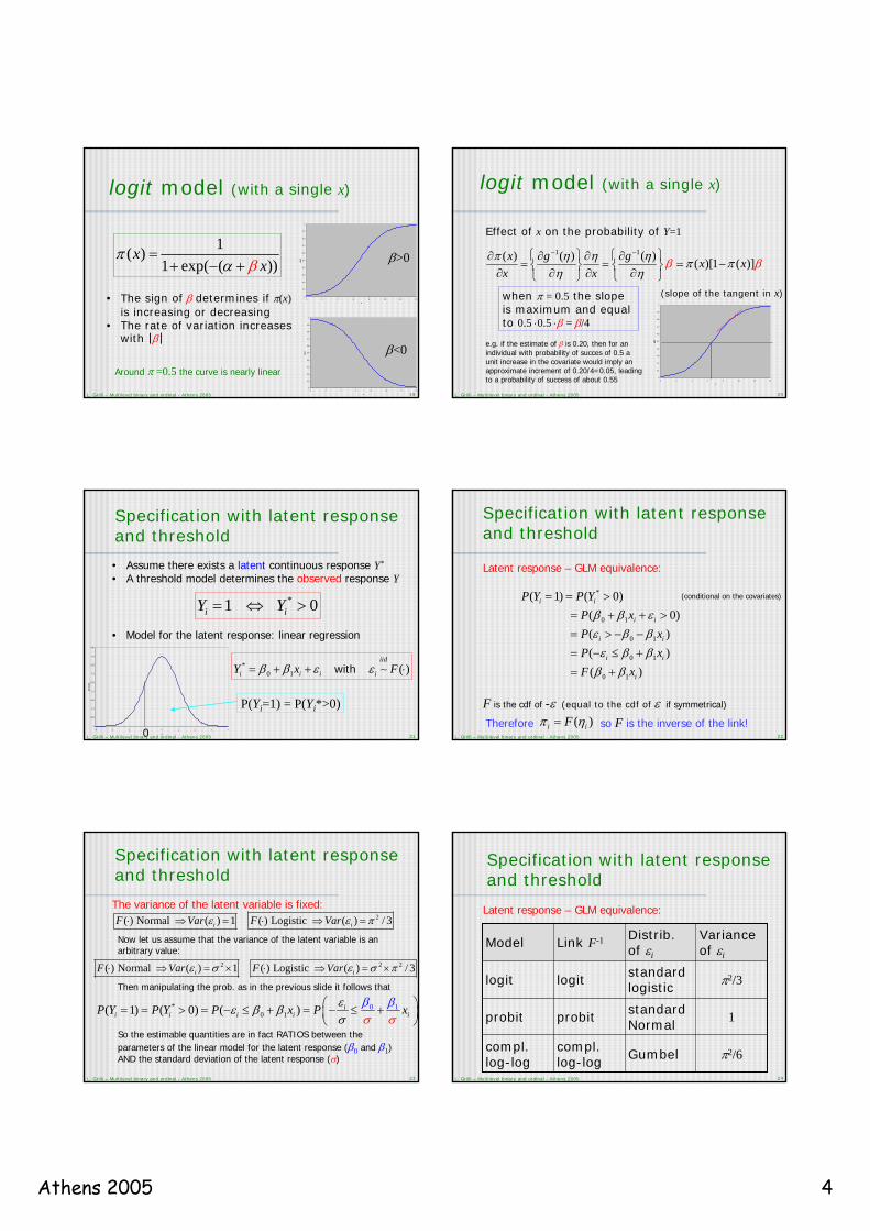
logit model (with a single x)
1( )1 exp( ( ))
xx
πα β
=+ − +
0
0.1
0.2
0.3
0.4
0.5
0.6
0.7
0.8
0.9
1
0 2 4 6 8 10 12 14
x
p(x) β>0
0
0.1
0.2
0.3
0.4
0.5
0.6
0.7
0.8
0.9
1
0 2 4 6 8 10 12 14
x
p(x) β<0
• The sign of β determines if π(x)is increasing or decreasing
• The rate of variation increases with |β|
Around π =0.5 the curve is nearly linear
20L. Grilli – Multilevel binary and ordinal - Athens 2005
logit model (with a single x)
0
0.1
0.2
0.3
0.4
0.5
0.6
0.7
0.8
0.9
1
0 2 4 6 8 10 12 14
x
p(x)
(slope of the tangent in x)when π = 0.5 the slope is maximum and equal to 0.5 ⋅0.5 ⋅β = β/4
1 1( ) ( ) ( ) ( )[1 ( )]x g g x xx x
π η η η β βπ πη η
− −⎧ ⎫ ⎧ ⎫∂ ∂ ∂ ∂= = = −⎨ ⎬ ⎨ ⎬∂ ∂ ∂ ∂⎩ ⎭ ⎩ ⎭
Effect of x on the probability of Y=1
e.g. if the estimate of β is 0.20, then for an individual with probability of succes of 0.5 a unit increase in the covariate would imply an approximate increment of 0.20/4=0.05, leading to a probability of success of about 0.55
21L. Grilli – Multilevel binary and ordinal - Athens 2005
Specification with latent response and threshold
*1 0i iY Y= ⇔ >
• Assume there exists a latent continuous response Y*
• A threshold model determines the observed response Y
P(Yi=1) = P(Yi*>0)0
0.05
0.1
0.15
0.2
0.25
0.3
0.35
0.4
0.45
-4 -3 -2 -1 0 1 2 3 4
y
dens
ità
• Model for the latent response: linear regression
0
*0 1 ( )
iid
i i i iY x Fβ β ε ε= + + ⋅with ∼
22L. Grilli – Multilevel binary and ordinal - Athens 2005
Specification with latent response and threshold
Latent response – GLM equivalence:
*
0 1
0 1
0 1
0 1
( 1) ( 0)( 0)( )( )( )
i i
i i
i i
i i
i
P Y P YP xP xP xF x
β β εε β β
ε β ββ β
= = >= + + >
= > − −
= − ≤ += +
( )i iFπ η=Therefore so F is the inverse of the link!
F is the cdf of -ε (equal to the cdf of ε if symmetrical)
(conditional on the covariates)
23L. Grilli – Multilevel binary and ordinal - Athens 2005
Specification with latent response and threshold
The variance of the latent variable is fixed:
Now let us assume that the variance of the latent variable is anarbitrary value:
2( ) Normal ( ) 1 ( ) Logistic ( ) / 3i iF Var F Varε ε π⋅ ⇒ = ⋅ ⇒ =
1*0 1
0( 1) ( 0) ( ) ii i i i iP Y P Y P x P xεε β β β β
σ σσ⎛ ⎞= = > = − ≤ + = − ≤ +⎜ ⎟⎝ ⎠
2 2 2( ) Normal ( ) 1 ( ) Logistic ( ) / 3i iF Var F Varε σ ε σ π⋅ ⇒ = × ⋅ ⇒ = ×
Then manipulating the prob. as in the previous slide it follows that
So the estimable quantities are in fact RATIOS between the parameters of the linear model for the latent response (β0 and β1) AND the standard deviation of the latent response (σ)
24L. Grilli – Multilevel binary and ordinal - Athens 2005
Specification with latent response and threshold
Latent response – GLM equivalence:
π2/6Gumbelcompl. log-log
compl. log-log
1standard Normal
probitprobit
π2/3standard logisticlogitlogit
Variance of εi
Distrib. of εi
Link F-1Model

Athens 2005 5
25L. Grilli – Multilevel binary and ordinal - Athens 2005
Specification with latent response and threshold
*1 i iY Y γ= ⇔ >An alternative specification
P(Yi=1) = P(Yi*> γ)
0
0.05
0.1
0.15
0.2
0.25
0.3
0.35
0.4
0.45
-4 -3 -2 -1 0 1 2 3 4
y
dens
ità
i.e. the threshold γ is not fixed to 0 but it is an estimable parameter. However a constraint on the model for Y* is needed
γ
*1 with ( )
iid
i i i iY x Fβ ε ε= + ⋅∼
To avoid collinearity (non identification)
the intercept of Y* is fixed to 0
26L. Grilli – Multilevel binary and ordinal - Athens 2005
Binary response:
multilevel logit model
27L. Grilli – Multilevel binary and ordinal - Athens 2005
Introduction to multilevel logit models
Definition
“cluster-specific” vs “population-average” effects
Random intercept model
ICC
Estimation
• Snijders & Bosker §14.1-14.2, 14.3.2-14.3.3• Skrondal & Rabe-Hesketh ch. 9
28L. Grilli – Multilevel binary and ordinal - Athens 2005
Random effects GLM for a binary response (GLMM)
Components of a GLMM (Generalized Linear Mixed Model)
1. GLM for the distribution of Y conditioned on the random effects
2. distribution of the random effects
Remark: the marginal distribution of Y (marginal w.r.t. the random effects) does not follow a GLM!!!
29L. Grilli – Multilevel binary and ordinal - Athens 2005
Random effects GLM for a binary response (GLMM)
(1) linear predictor
(2) logit link
(3) distribution
• The β are the conditional effects of the covariates, given the value of the random effects u cluster specific effects
• The marginal effects of the covariates are obtained integratingw.r.t. the random effects u
'ij ij juη = +x βlogit( )ij ijµ η=
| , (1, )iid
ij ij j ijY u Bin πx ∼
individual i =1,2,…,nj; cluster: j =1,2,…,J
GLM forY|u
f(u) 2(0, )iid
j uu N σ∼
30L. Grilli – Multilevel binary and ordinal - Athens 2005
cluster-specific vs population-average effects
( )0 1
1( 1| , )1 exp ( )jij
i jij
j
uxu
P Yxβ β
= =+ − + +
cluster-specificmodel (random intercept)
( )0 1
1( 1| )1 exp ( )ij ij
ij
P Y xxγ γ
= =+ − +
γ1 < β1
the effect of x is attenuated!
see Skrondal & Rabe-Hesketh §4.8and the paper of Ritz & Spiegelman
0
0.1
0.2
0.3
0.4
0.5
0.6
0.7
0.8
0.9
1
0 10 20 30 40 50 60 70 80 90 100
population-averagemodel (constant intercept)

Athens 2005 6
31L. Grilli – Multilevel binary and ordinal - Athens 2005
Estimating conditional probabilities
( )0 1
1
1 exp ( )( 1| , )
jij
jij ij uxP Y x u
β β+ − + += =
choose a value of xijplug-in the estimates of the fixed effectschoose a value of uj , for example
zero → hypothetical mean clustera low value (e.g. ) → hypothetical “bad” clustera high value (e.g. ) → hypothetical “good” clusteran EB residual → j-th cluster of the sample
Fit the random effects model and
0 1ˆ , ˆβ β
ˆ2 uσ−ˆ2 uσ+
ˆEBju
32L. Grilli – Multilevel binary and ordinal - Athens 2005
Estimating marginal probabilities
( )0 1ˆ
1ˆ ( 1 | )1 exp ˆ( )
ij ij
ij
P Y xxγ γ
= =+ − +
1) fit a model random effects (population - averaged)
and plug - in the estimates
without
( 1| )ij ijP Y x=Two ways to estimate
( )0 1
2
ˆ ( 1 | )1
1 exp ( )ˆ ˆ
ˆ ( 1| , )
( ;0 ˆ, )
ij ij
ij
i
uj jj
j ij jP Y x E
x
u
uu
P Y x
duβ
φβ
σ=
= =
+ − + +
⎡ ⎤=⎣ ⎦
∫
2) fit a model random effects (cluster - specific), plug - in the estimates and compute the integral
withor
33L. Grilli – Multilevel binary and ordinal - Athens 2005
Null random intercept logit model
population mean of logits or logit of the mean cluster
uj ~N(0,σu2)
( )0
0
1( 1| )1 exp ( )
logit( ) log1
j ij
jj
j
jj
j
uu
u
P Yπ
ππ
β
βπ
= = =+ − +
⎛ ⎞= = +⎜ ⎟⎜ ⎟−⎝ ⎠
0β
34L. Grilli – Multilevel binary and ordinal - Athens 2005
Random intercept logit model with covariates
( )0 1
0 1
1( 1| , )1 exp ( )
logit( ) log1
jj
ij ij ijij
ijij ij
ij
j
P Y xx
x
uu
u
π
ππ
β β
β βπ
= = =+ − + +
⎛ ⎞= = + +⎜ ⎟⎜ ⎟−⎝ ⎠
• Cluster-level covariates can be inserted• Individual-level covariates can have a random coefficient• Cross-level interaction terms can be inserted
35L. Grilli – Multilevel binary and ordinal - Athens 2005
ICC in binary response models
Specification with a continuous latent response
The total error uj+εij has variance:σu
2 +1 in the probit modelσu
2 +π2/3 in the logit model
The (residual) ICC is the between/total variance ratio:ρ = σu
2 /(σu2 +1) in the probit model
ρ = σu2 /(σu
2 +π2/3) in the logit model
0*
1ij ij ij jY x uβ β ε= + + +
2(0, )iid iid
u ijj N Fu σ ε∼ ∼
36L. Grilli – Multilevel binary and ordinal - Athens 2005
ICC in binary response models
For two individuals of the same cluster, the two responses are conditionally indipendent given the random effects:
Marginally w.r.t. the random effects, the correlation (in the latent responses) between the same two individuals is equal to the (residual) ICC:
* *' '( , | , , ) 0ij i j ij i j jCorr Y Y x x u =
* *' '( , | , )ij i j ij i jCorr Y Y x x ρ=
Athens 2005 7
37L. Grilli – Multilevel binary and ordinal - Athens 2005
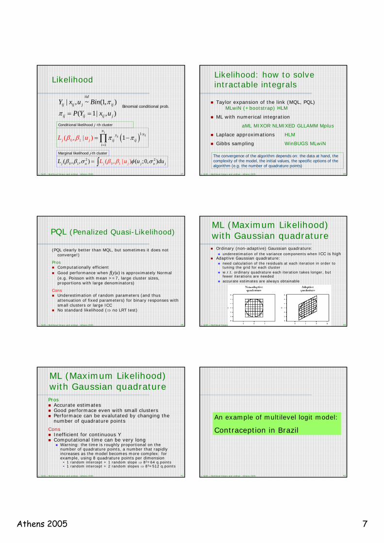
Likelihood
21 0 1
20 (( , , ) ( ;0, | ) , )j u j u jj jL u u duL β ββ β σ φ σ= ∫
Binomial conditional prob.
Marginal likelihood j-th cluster
Conditional likelihood j -th cluster
( )1-
11
0 1( , | )j
ijij
nyy
ij ijj ji
L u πβ πβ=
= −∏
| , ~ (1, )
( 1| , )
iid
ij ij j ij
ij ij ij j
Y x u Bin
P Y x u
π
π = =
38L. Grilli – Multilevel binary and ordinal - Athens 2005
Likelihood: how to solve intractable integrals
Taylor expansion of the link (MQL, PQL)MLwiN (+bootstrap) HLM
ML with numerical integration
aML MIXOR NLMIXED GLLAMM Mplus
Laplace approximations HLM
Gibbs sampling WinBUGS MLwiN
The convergence of the algorithm depends on: the data at hand, the complexity of the model, the initial values, the specific options of the algorithm (e.g. the number of quadrature points)
39L. Grilli – Multilevel binary and ordinal - Athens 2005
PQL (Penalized Quasi-Likelihood)
(PQL clearly better than MQL, but sometimes it does not converge!)
ProsComputationally efficientGood performance when f(y|u) is approximately Normal(e.g. Poisson with mean >=7, large cluster sizes,proportions with large denominators)
ConsUnderestimation of random parameters (and thus attenuation of fixed parameters) for binary responses with small clusters or large ICCNo standard likelihood (⇒ no LRT test)
40L. Grilli – Multilevel binary and ordinal - Athens 2005
ML (Maximum Likelihood) with Gaussian quadrature
Ordinary (non-adaptive) Gaussian quadrature:underestimation of the variance components when ICC is high
Adaptive Gaussian quadrature:need calculation of the residuals at each iteration in order to tuning the grid for each clusterw.r.t. ordinary quadrature each iteration takes longer, but fewer iterations are neededaccurate estimates are always obtainable
41L. Grilli – Multilevel binary and ordinal - Athens 2005
ML (Maximum Likelihood) with Gaussian quadraturePros
Accurate estimatesGood performace even with small clustersPerformace can be evalutated by changing the number of quadrature points
ConsInefficient for continuous YComputational time can be very long
Warning: the time is roughly proportional on the number of quadrature points, a number that rapidly increases as the model becomes more complex: for example, using 8 quadrature points per dimension
• 1 random intercept + 1 random slope ⇒ 82=64 q.points• 1 random intercept + 2 random slopes ⇒ 83=512 q.points
42L. Grilli – Multilevel binary and ordinal - Athens 2005
An example of multilevel logit model:
Contraception in Brazil
Athens 2005 8
43L. Grilli – Multilevel binary and ordinal - Athens 2005
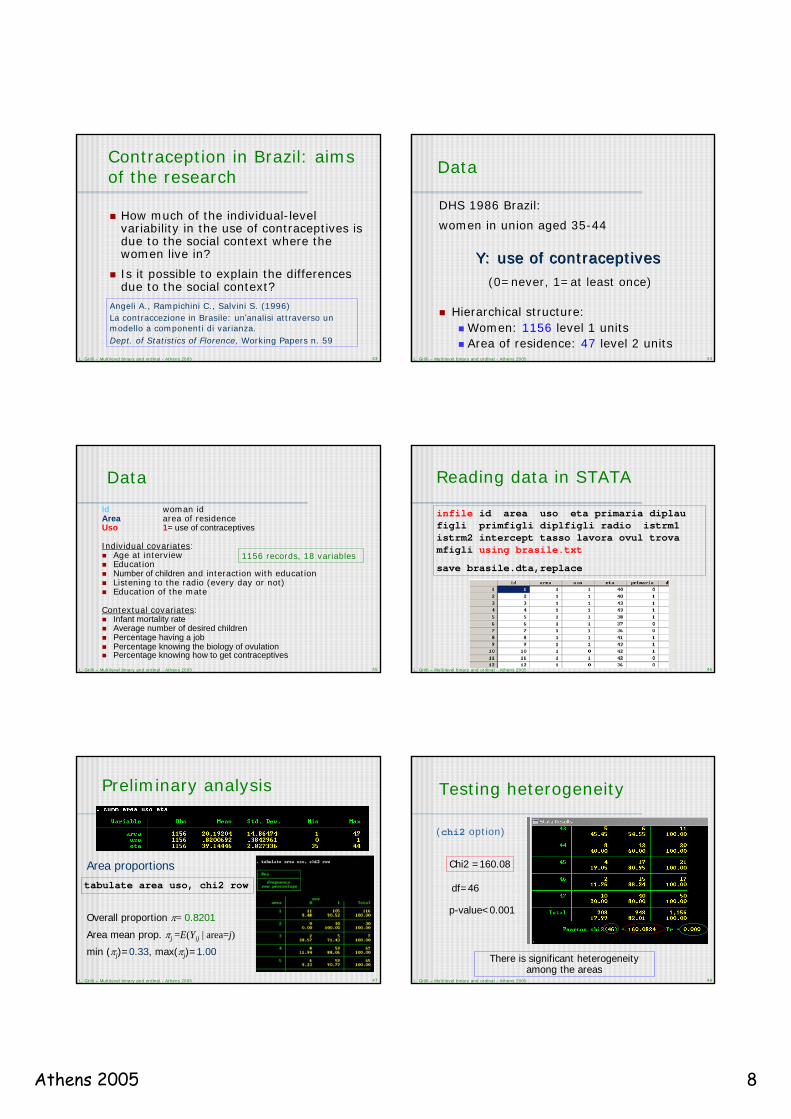
Contraception in Brazil: aims of the research
How much of the individual-level variability in the use of contraceptives is due to the social context where the women live in?
Is it possible to explain the differences due to the social context?
Angeli A., Rampichini C., Salvini S. (1996)La contraccezione in Brasile: un’analisi attraverso un modello a componenti di varianza.Dept. of Statistics of Florence, Working Papers n. 59
44L. Grilli – Multilevel binary and ordinal - Athens 2005
Data
DHS 1986 Brazil:
women in union aged 35-44
Y: Y: use of contraceptivesuse of contraceptives
(0=(0=never,never, 1=1=at least onceat least once))
Hierarchical structure:Women: 1156 level 1 unitsArea of residence: 47 level 2 units
45L. Grilli – Multilevel binary and ordinal - Athens 2005
Data
Id woman idArea area of residenceUso 1= use of contraceptives
Individual covariates:Age at interviewEducationNumber of children and interaction with educationListening to the radio (every day or not)Education of the mate
Contextual covariates:Infant mortality rateAverage number of desired childrenPercentage having a jobPercentage knowing the biology of ovulationPercentage knowing how to get contraceptives
1156 records, 18 variables
46L. Grilli – Multilevel binary and ordinal - Athens 2005
Reading data in STATA
infile id area uso eta primaria diplau figli primfigli diplfigli radio istrm1 istrm2 intercept tasso lavora ovul trova mfigli using brasile.txt
save brasile.dta,replace
47L. Grilli – Multilevel binary and ordinal - Athens 2005
Preliminary analysis
Area proportions
Overall proportion π= 0.8201
Area mean prop. πj =E(Yij | area=j)
min (πj)=0.33, max(πj)=1.00
tabulate area uso, chi2 row
48L. Grilli – Multilevel binary and ordinal - Athens 2005
Testing heterogeneity
p-value<0.001
There is significant heterogeneity among the areas
Chi2 =160.08
df=46
(chi2 option)

Athens 2005 9
49L. Grilli – Multilevel binary and ordinal - Athens 2005
Null model with GLLAMM
gllamm uso, i(area) family(binomial) link(logit) nip(5) adapt trace dots
yij~Bin(1,πij)
uso : response variablearea : variable identifying level 2 unitsnip(5) adapt : 5-point adaptive quadrature
logit(πij)=β0+ujSort the data
Model specification
sort area id
50L. Grilli – Multilevel binary and ordinal - Athens 2005
σu2 variance between
areas
Results of null model
1/[1+exp(-β0)]=0.8318
matrix a=e(b)
matrix list adi exp(a[1,1])/(1+exp(a[1,1]))
Estimated probability for uj=0
different from E(πj)!
β0
πj for high u: 1/[1+exp(β0 +2σu)]= 0.9680πj for low u: 1/[1+exp(β0 –2σu)]= 0.4473
51L. Grilli – Multilevel binary and ordinal - Athens 2005
Model with radio
Inserting radio (fixed effect)
( )0 1
0 1
1P( 1| )1 exp
logit( ) log1
ij j ijij j
ijij ij j
ij
Y ux u
x u
πβ β
ππ β β
π
= = =⎡ ⎤+ − + +⎣ ⎦
⎛ ⎞= = + +⎜ ⎟⎜ ⎟−⎝ ⎠
gllamm uso radio, i(area)family(binomial) link(logit) nip(5) adapt from(a) trace dots
Initial values from previous model52L. Grilli – Multilevel binary and ordinal - Athens 2005
Results of model with radio
Between variance: nearly the same as before
Better model fitLRT=2*(517.55307-509.8697)=15.4
radio=0 1/(1+exp(-_b[_cons])) =0.76
radio=1 1/(1+exp(-_b[_cons]-_b[_radio])) =0.86
Estimated probability using contraceptives for uj=0
53L. Grilli – Multilevel binary and ordinal - Athens 2005
Odds
For x=1 and u=0 the odds of Y=1 is
π(1)/[1-π(1)]=exp(β0 + β1)
=exp(1.1596+0.6835)= 6.316
for a women listening to the radio every day and living in a mean area, it is about 6 timesmore probable to use contraceptives than to not use
54L. Grilli – Multilevel binary and ordinal - Athens 2005
Odds
Mean area (u=0)exp(1.1596+0.6835)= 6.316
Low area (u=-2σu)exp(1.1596+0.6835-2*0.8939)= 1.057
High area (u=+2σu)exp(1.1596+0.6835+2*0.8939)= 37.75
05
10152025303540
-2 -1.5 -1 -0.5 0 0.5 1 1.5 2
u
odds
(rad
io=1
)
For x=1 the odds of Y=1 is a function of uπ(1|u)/[1-π(1|u)]=
exp(β0 + β1+ u)

Athens 2005 10
55L. Grilli – Multilevel binary and ordinal - Athens 2005
Odds Ratio
OR=(π(1)/[1-π(1)])/(π(0)/[1-π(0)])=exp(β)
log OR =β
OR is a measure of association between Y and Xwhich does not depend on u
OR(radio)=1.9838
The use of contraceptives is about 2 times more probable for a woman listening to the radio every day (whichever area she lives in)
56L. Grilli – Multilevel binary and ordinal - Athens 2005
Inserting other covariates
0.0070.02414893.89contextual
0.1600.62811934.69individual0.1960.80331019.78radio
0.2020.83121035.15null
ρσu2n.par.-2logLmodel
Residual ICC (on the latent response):
(fitted with MIXOR)
2* *
' ' 2 2( , | , )/ 3
uij i j ij i j
u
Corr Y Y x xσ
ρ σπ
= =+
57L. Grilli – Multilevel binary and ordinal - Athens 2005
Ordinal response:
standard proportional odds model
58L. Grilli – Multilevel binary and ordinal - Athens 2005
Ordinal responses
Y can assume C distinct values(categories) yc c=1,2,…,C
The categories are ordered
y1 < y2 <…< yc <…< yC
As a convention, the category yc is labelled with the number c
Examples:Severity of the symptoms: none, light, seriousResult of a test: normal, borderline, anormalSatisfaction: low, intermediate, high
59L. Grilli – Multilevel binary and ordinal - Athens 2005
Probabilities to be modelled
( 1)( 2)
(
(
1)
) 1
P YP Y
P Y C
P Y C≤ =
≤≤
≤ −……
1
1
( ) 1 ( )
( 1)( 2)
( 1)C
c
P Y C P Y
P YP Y
P C
c
Y−
=
= = − =
==
= −
∑
……
With C categories there are C-1 free probabilities, e.g. the first C-1 mass points of the distribution, or the first C-1 cumulative probabilities of the distribution
60L. Grilli – Multilevel binary and ordinal - Athens 2005
Cumulative GLM
Given the ordinal nature of Y it is convenient to build the model on the cumulative probabilities
Following the GLM approach
' linear predictor (stesso per tutte le prob. cumulate)specific intercept ( ) of the -th cumulative prob.
( ) link function
i i
c cthresholdg
ηγ
=
⋅
β x
( )( ) 1, , 1ci icg P Y c Cγ η≤ = − = −…
A cumulative GLM for an ordinal Y with C categories is made of C-1 submodels, one for each cumulative prob. (except the last one)

Athens 2005 11
61L. Grilli – Multilevel binary and ordinal - Athens 2005
Cumulative GLM
1 2 1Cγ γ γ −≤ ≤ ≤…
( )( ) 1, , 1ci icg P Y c Cγ η≤ = − = −…
What is the relationship among the C-1 thresholds γc ?
As the cumulative probabilities are non-decreasing by construction, also the thresholds must be be non-decreasing
Why the linear predictor has a minus sign?
To interpret the coefficients in the usual way: in fact, with the minus sign, increasing the value of a covariate with a positivecoefficient amounts to increasing the probability of a high category (i.e. a category in the right end of the scale)
62L. Grilli – Multilevel binary and ordinal - Athens 2005
Cumulative GLM
( )( ) 1, , 1ci icg P Y c Cγ η≤ = − = −…
How to compute the probability of a specific category c ?
By difference (hence the name difference model):
( ) ( )11 1
( ) ( ) ( )1i i i
ci ic
c c cP Y P Y P Y
g gγ η γ η−−
−
−= = ≤ − ≤
= − − −
63L. Grilli – Multilevel binary and ordinal - Athens 2005
Cumulative GLM
( )( ) 1, , 1ci icg P Y c Cγ η≤ = − = −…
What is the consequence of having the same linear predictor for all the categories?
A given covariate has an effect on the cumulative probabilities equal for all the categories of Y (so called parallel regressions assumption)
Such an assumption is clearly violated for a covariate that is not associated with a shift in the scale, but rather with an “extremization” of the responses (e.g. the individuals with certain features might use only the extremes of the scale)
64L. Grilli – Multilevel binary and ordinal - Athens 2005
Logit cumulative GLM: the proportional odds model
( )( ) 1, , 1ci icg P Y c Cγ η≤ = − = −…If g() is the logit function, the cumulative GLM is called “proportional odds”. The odds of exceeding category c are
( )( )
1 1/ 1 exp( ( ' )( ) 1 ( )( ) ( ) 1/ 1 exp( ( ' )
exp( ( ' ) exp( ' )
c
c
c c
ii i
i i i
i i
P Y P Y cY P
cc cP Y
γγ
γ γ
− + − −> − ≤= =
≤ ≤ + − −
= − − = −
β xβ x
β x β x
Similarly, the odds of not exceeding category c are
( ) exp( ' )( )
i
ic i
P YP Y
cc
γ≤= −
>β x Same expression but
with reversed signs!
65L. Grilli – Multilevel binary and ordinal - Athens 2005
Logit cumulative GLM: the proportional odds model
With reference to the odds of exceeding a category (or equivalently the odds of not exceeding), any two individuals have proportional odds, i.e. the ratio of the odds is the same for all the categories of Y
Let us consider two individuals A and B with the same values of the covariates with the exception of the r-th covariate, for which individual B has a value exceeding by 1 the value of individual A, so the difference in the linear predictor is
With reference to the odds of exceeding a category
exp( ' )( ) / ( ) exp(( ' ) ( ' )) exp( )( ) / ( ) exp( ' )
BB BB A r
A A
cc c
cA
c cc
P Y P YP P Y cY
γ γ γ βγ
−> ≤= = − − − =
> ≤ −β x β x β xβ x
' 'B A rβ− =β x β x
So the Odds Ratio is exp(βr) for any category c: this is the proportional odds property!
66L. Grilli – Multilevel binary and ordinal - Athens 2005
Specification with latent response and a set of thresholds
{ } { }1* c- i ciY Yc γ γ= ⇔ < ≤
• Underlying the observed value Y for the i-th individual there is a continuous latent response Y*
• A threshold mechanism determines the observed response:
0
0.05
0.1
0.15
0.2
0.25
0.3
0.35
0.4
0.45
-4 -3 -2 -1 0 1 2 3 4
y
dens
ità
• The latent response is modelled with a linear regression model without intercept:
* 'iid
i i i iY Fε ε= +β x ∼
( ) ( )1*
c-i i cP Y P Yc γ γ= = < ≤

Athens 2005 12
67L. Grilli – Multilevel binary and ordinal - Athens 2005
Specification with latent response and a set of thresholds
A latent response model is equivalent to a cumulative GLM:
( ) ( ) ( )( ) ( )
* '
' 'ci i i i
i i i
c
c c
P Y c P Y P
P F
γ ε γ
ε γ γ
≤ = ≤ = + ≤
= ≤ − = −
β x
β x β x
This relationship makes clear why in a cumulative GLM the estimated regression coefficients are approximately invariant to collapsing of the categories (warning: in principle the invariance is perfect, but in practice if the model is not adequate for the data at hand the estimates may change a lot)
68L. Grilli – Multilevel binary and ordinal - Athens 2005
Specification with latent response and a set of thresholds
Latent response – GLM equivalence:
π2/6Gumbelcompl. log-log
ordinal c. log-log
1standard Normal
probitordinal probit
π2/3standard logisticlogitproportional
odds
Variance of εi
Distrib. of εi
Link F-1Model
69L. Grilli – Multilevel binary and ordinal - Athens 2005
Ordinal response:
multilivel proportional odds model
70L. Grilli – Multilevel binary and ordinal - Athens 2005
Random intercept two-level ordinal response model
Representation with continuous latent response and a set of thresholds
* ' iji ijjj uY ε+= +β x2(0, )
iid iid
j u iju N Fσ ε∼ ∼Estimable parameters:• regression coefficients β (same number as the covariates)• level 2 variance: σu
2
• C-1 thresholds: γ1,…,γC-1
71L. Grilli – Multilevel binary and ordinal - Athens 2005
ICC in ordinal response models
Representation with a continuous latent response
The total error uj+εij has variance:σu
2 +1 in the ordinal probit modelσu
2 +π2/3 in the proportional odds model
The (residual) ICC is the between/total variance ratio:ρ = σu
2 /(σu2 +1) in the ordinal probit model
ρ = σu2 /(σu
2 +π2/3) in the proportional odds model
0*
1ij iij j jx uY εβ β+ ++=
2(0, )iid iid
j u iju N Fσ ε∼ ∼
72L. Grilli – Multilevel binary and ordinal - Athens 2005
ICC in ordinal response models
For two individuals of the same cluster, the two responses are conditionally indipendent given the random effects:
Marginally w.r.t. the random effects, the correlation (in the latent responses) between the same two individuals is equal to the (residual) ICC:
* *' '( , | , , ) 0ij i j ij i j jCorr Y Y x x u =
* *' '( , | , )ij i j ij i jCorr Y Y x x ρ=

Athens 2005 13
73L. Grilli – Multilevel binary and ordinal - Athens 2005
Multilevel ordinal response models
The issues that arise when introducing random effects in an ordinal response model are the same already noted in the binary response case, e.g.
cluster-specific vs. population-average effectsmarginal vs. conditional probabilitiesestimation algorithms approximating the integrals
Snijders & Bosker §14.4, Skrondal & Rabe-Hesketh ch. 10
74L. Grilli – Multilevel binary and ordinal - Athens 2005
Example of multilevel proportional odds model:
Tobacco information programme TVSFP
75L. Grilli – Multilevel binary and ordinal - Athens 2005
Tobacco information programme TVSFP
Data collected during the programme “TelevisionSchool and Family Smoking Prevention andCessation”
The schools in the sample were randomized to 4 types of treatment defined by crossing two factors:
CC dummy indicator for classroom interventionTV dummy indicator for television intervention
Hierarchical structure: students in classes, classesin schools
Hedeker and Gibbons (1996), MIXOR manual Rabe-Hesketh et al. (2004), GLLAMM manual
76L. Grilli – Multilevel binary and ordinal - Athens 2005
Ordinal response model
Response variable THK
------------thk | Freq.----+-------
1 | 2592 | 2773 | 2694 | 294
------------
Score defined as the number of correct answers to 7 questions on tobacco knowledge after the intervention, collapsed into 4 categories (higher means better knowledge)
77L. Grilli – Multilevel binary and ordinal - Athens 2005
Ordinal response model
CovariatesCC indicator for classroom interventionTV indicator for television interventionCCTV interaction CC*TVPRETHK pre-intervention value of THK
Variable | Obs Mean Std. Dev. Min Max----------+---------------------------------------------
prethk | 1600 2.069375 1.26018 0 6cc | 1600 .476875 .4996211 0 1tv | 1600 .499375 .5001559 0 1
CC and TV are randomized at school level
78L. Grilli – Multilevel binary and ordinal - Athens 2005
Reading and collapsing the data
When both the response and the covariates can assume few distinct values there are several individuals with the same value for Y and x
Collapsing reduces the size of the dataset and thus the computational time
gen cons=1collapse (count) wt1=cons, by(thk prethk
cc tv cctv School class)
infile school class thk a2 const prethk cctv cctv using tvsfpors.dat

Athens 2005 14
79L. Grilli – Multilevel binary and ordinal - Athens 2005
Two-level ordinal model:students in classes
ηijk=β0+β1PRETHKijk+ β2CCk + β3TVk + β4CCTVk + ujk
ujk ~N(0,τ2), i student, j class, k school
Response THKF
Linear predictor
gllamm thk prethk cc tv cctv, i(class)family(binomial) link(ologit)weight(wt) nip(10) trace dots
Ordinal logit linkWeights corresponds to level 1 units (students)
80L. Grilli – Multilevel binary and ordinal - Athens 2005
Results The level of knowledge before intervention (prethk) is a good predictor of the knowledge after intervention
Only the classroom intervention (CC) has an effect
3 thresholds(Y has 4 categories)
Variance between classes=0.1888, ρ=0.1888/(0.1888+π2/3)=0.054
81L. Grilli – Multilevel binary and ordinal - Athens 2005
Checking the performance of Gaussian quadrature
• Fit the model again with more quadrature points• Fit the model again with adaptive quadrature
(option adapt)Otherwise a quick method is to
• Evaluate the likelihood using more quadrature points (option eval)
In the TVSFP data the logL is about the same using 20 and 30 points the approximation yielded by 10-point quadrature seem to be adequate
82L. Grilli – Multilevel binary and ordinal - Athens 2005
Dropping TV and CCTV
estimates store a
matrix a=e(b)
gllamm thk prethk cc, i(class) family(binomial) link(ologit)weight(wt) nip(10) from(a) trace
Save the results of previous model
Initial values from the previous model
83L. Grilli – Multilevel binary and ordinal - Athens 2005
Interpretation of the parameters:odds ratio
Example: odds ratio of CC=1 on CC=0 conditions being equal on PRETHK and ujk
( 1) [thk]cc = 0-----------------------------------------------------------thk | exp(b) Std. Err. z P>|z| [95% Conf. Interval]----+-------------------------------------------------------(1) | 2.04235 .2562923 5.69 0.000 1.597033 2.61184------------------------------------------------------------
It does not depend on the threshold c!
( | 0) / ( | 0)Odds Ratio of B on A exp( )
( | 0) / ( | 0)B jk B jk
rA jk A jk
P Y u P Y uP Y u P
c cY uc c
β> = ≤ =
= => = ≤ =
A and B with the same covariate values with the exception of the r-th covariate, for which unit B has a value exceeding 1 that of unit A
lincom cc, eform
84L. Grilli – Multilevel binary and ordinal - Athens 2005
Interpretation of the parameters:odds of exceeding a category
lincom [thk]cc - [_cut11]_cons, eform
Example: for a student with PRETHKijk=0, CCk=1 and ujk=0 the odds of exceeding category c=1 is
( 1) [thk]cc - [_cut11]_cons = 0------------------------------------------------------------thk | exp(b) Std. Err. z P>|z| [95% Conf. Interval]----+-------------------------------------------------------(1) | 2.43737 .2963014 7.33 0.000 1.920633 3.093134------------------------------------------------------------
Similarly, for c=2 odds=0.68, c=3 odds=0.20
( ) exp( ' )( )
ii
ic
P YP Y
cc
γ>= −
≤β x

Athens 2005 15
85L. Grilli – Multilevel binary and ordinal - Athens 2005
Interpretation of the parameters:probability of a category
( )( ) ( )( )
*1
1* *
1
( | 0) ( | 0)
( | 0) ( | 0)
1/ 1 exp ( ' ) 1/ 1 exp ( ' )
ij jk ijk jk
ijk jk ijk jk
ijk ijk
c c
c c
c c
P Y u P Y u
P Y u P Y
c
u
γ γ
γ γ
γ γ
−
−
−
= = = < ≤ =
= ≤ = − ≤ =
= + − − − + − −β x β x
Category CC=0 CC=11 0.46 0.292 0.29 0.303 0.16 0.244 0.09 0.17TOT 1.00 1.00
E.g. PRETHKijk=0 and ujk=0
86L. Grilli – Multilevel binary and ordinal - Athens 2005
Two-level ordinal model:students in classes in schools
gllamm thk prethk cc tv cctv, i(classschool) family(binomial) link(ologit)weight(wt) nip(10) trace
LRT shows that the variance between schools is not significant ⇒ school level can be dropped
ηijk=β0+β1PRETHKijk+ β2CCk + β3TVk + β4CCTVk + ujk +vk
ujk ~N(0,τ2), vk ~N(0,ψ2), i student, j class, k school


