
Technische Universitat Munchen
Fakultat fur Informatik
Lehrstuhl VII: Theoretische Informatik
Multi-Task and Transfer Learningwith Recurrent Neural Networks
Sigurd Spieckermann
Vollstandiger Abdruck der von der Fakultat fur Informatik der Technischen
Universitat Munchen zur Erlangung des akademischen Grades eines
Doktors der Naturwissenschaften (Dr. rer. nat.)
genehmigten Dissertation.
Vorsitzender: Univ.-Prof. Dr. Dr. h.c. Javier Esparza
Prufer der Dissertation: 1. Hon.-Prof. Dr.-Ing. Thomas A. Runkler
2. Univ.-Prof. Dr. Patrick van der Smagt
Die Dissertation wurde am 19.05.2015 bei der Technischen Universitat Munchen
eingereicht und durch die Fakultat fur Informatik am 28.09.2015 angenommen.

Abstract
Being able to obtain a model of a dynamical system is useful for a variety of
purposes, e.g. condition monitoring and model-based control. The dynamics of
complex technical systems such as gas or wind turbines can be approximated by
data driven models, e.g. recurrent neural networks. Such methods have proven
to be powerful alternatives to analytical models which are not always available or
may be inaccurate. Optimizing the parameters of data-driven models generally
requires large amounts of operational data. However, data is a scarce resource
in many applications, hence, data-efficient procedures utilizing all available data
are preferred.
In this thesis, recurrent neural networks are explored and developed which
allow for data-efficient knowledge transfer from one or multiple source tasks to
a related target task that lacks sufficient amounts of data. Multiple knowledge
transfer scenarios are considered: dual-task learning, multi-task learning, and
transfer learning. Dual-task learning is a particular case of multi-task learn-
ing in which multiple tasks are learned simultaneously, thus, allowing to share
knowledge among the tasks. Transfer learning implies a sequential protocol in
which the target task is learned subsequent to learning one or multiple source
tasks. Knowledge transfer is explored and applied in the context of fully and
partially observable system identification to improve the model of a little ob-
served system by means of auxiliary data from one or multiple similar systems.
Fully observable system identification assumes that the observed system state
corresponds to the true state while partial observability implies the observation
of either a subset of the state variables or proxy variables.
The primary contribution of this thesis comprises a novel recurrent neural net-
work architecture for knowledge transfer which uses factored third-order tensors
to encode cross-task and task-specific information within composite affine trans-
formations. This model is investigated in a series of experiments on synthetic
iii

as well as real-world gas turbine data. Empirically, the proposed Factored Ten-
sor Recurrent Neural Network architecture outperforms the other considered
methods consistently in all experiments by transferring information from one or
multiple well-observed source task(s) to a little observed target task. Without
any transfer approach, the target task cannot be modeled successfully because
of insufficient amounts of available data. Besides this empirically proven merit,
the proposed Factored Tensor Recurrent Neural Network is appealing due to its
principal approach of incorporating cross-task and task-specific information into
the architecture, thereby, allowing for task-specific adaptation in a data-efficient
way.
iv

Acknowledgments
I would like to thank the “Learning Systems” research group at Siemens AG,
Corporate Technology, in Munich, Germany, for supporting this work. In par-
ticular, I would like to thank my supervisors, Thomas Runkler and Steffen
Udluft, for their guidance and support as well as proofreading the papers and
this thesis. My gratitude extends to the head of “Learning Systems”, Volkmar
Sterzing, who enabled my research in his group. I would also like to thank
Alexander Hentschel for the many enlightening conversations, both technical
and more general in nature, and his extraordinarily accurate proofreading of
the papers that he co-authored as well as part of this thesis. Further thanks go
to Siegmund Dull for his advice and support, particularly in familiarizing my-
self with the internal “Learning Systems” code base, which I used for generating
data for the experiments. I am grateful to Andrew Ng whose machine learning
course I took at Stanford University in 2011. His fascination for machine learn-
ing as well as his unique ability to teach the material in an outstandingly clear
and concise way sparked my passion for machine learning motivating me to dive
deeper into this field myself.
I particularly thank my parents, Helga and Rainer Spieckermann, who have
constantly supported and encouraged me in my personal and academic devel-
opment in many ways—morally, advisory, financially, etc. They laid the foun-
dation for all that I have become and that enabled this thesis. Last but not
least, I would like to express my gratitude to my fiancee, Caroline Roeger, who
has been by my side unconditionally despite the difficult times when we were
having a long-distance relationship during my studies in the U.S. and later when
I moved to Munich to pursue my PhD.
v

vi
Contents
Abstract iii
Acknowledgements v
1 Introduction 1
1.1 Contributions . . . . . . . . . . . . . . . . . . . . . . . . . . . . 4
1.2 Overview of the Thesis . . . . . . . . . . . . . . . . . . . . . . . 6
2 Theoretical Background 9
2.1 Machine Learning . . . . . . . . . . . . . . . . . . . . . . . . . . 9
2.2 Knowledge Transfer . . . . . . . . . . . . . . . . . . . . . . . . . 13
2.2.1 Formal Definition . . . . . . . . . . . . . . . . . . . . . . 14
2.2.2 Aspects of Transfer . . . . . . . . . . . . . . . . . . . . . 15
2.2.3 Settings . . . . . . . . . . . . . . . . . . . . . . . . . . . 16
2.2.4 Approaches . . . . . . . . . . . . . . . . . . . . . . . . . 17
2.2.5 Discussion . . . . . . . . . . . . . . . . . . . . . . . . . . 18
2.3 Neural Networks . . . . . . . . . . . . . . . . . . . . . . . . . . 19
2.3.1 Perceptron . . . . . . . . . . . . . . . . . . . . . . . . . . 19
2.3.2 Multi-Layer Perceptron . . . . . . . . . . . . . . . . . . . 20
2.3.3 Recurrent Neural Networks . . . . . . . . . . . . . . . . 22
2.4 Learning & Optimization . . . . . . . . . . . . . . . . . . . . . . 26
2.4.1 Backpropagation . . . . . . . . . . . . . . . . . . . . . . 26
2.4.2 Hessian-Free Optimization . . . . . . . . . . . . . . . . . 30
2.4.3 Overfitting . . . . . . . . . . . . . . . . . . . . . . . . . . 33
2.5 Hidden Markov Models . . . . . . . . . . . . . . . . . . . . . . . 35
2.6 Tensor Factorization . . . . . . . . . . . . . . . . . . . . . . . . 38
2.6.1 Tensors . . . . . . . . . . . . . . . . . . . . . . . . . . . 38
vii

Contents
2.6.2 Parallel Factor Analysis . . . . . . . . . . . . . . . . . . 39
2.6.3 Applications . . . . . . . . . . . . . . . . . . . . . . . . . 40
2.7 System Identification . . . . . . . . . . . . . . . . . . . . . . . . 42
2.8 Artificial Benchmarks . . . . . . . . . . . . . . . . . . . . . . . . 43
2.8.1 Cart-Pole . . . . . . . . . . . . . . . . . . . . . . . . . . 43
2.8.2 Mountain Car . . . . . . . . . . . . . . . . . . . . . . . . 44
2.9 Implementation . . . . . . . . . . . . . . . . . . . . . . . . . . . 45
3 Multi-Task and Transfer Learning with Recurrent Neural Net-
works 49
3.1 Multi-Task Learning . . . . . . . . . . . . . . . . . . . . . . . . 50
3.2 Multi-Task vs. Transfer Learning . . . . . . . . . . . . . . . . . 51
3.3 Multi-Task Recurrent Neural Networks . . . . . . . . . . . . . . 51
3.3.1 Naıve RNN . . . . . . . . . . . . . . . . . . . . . . . . . 52
3.3.2 RNN+ID . . . . . . . . . . . . . . . . . . . . . . . . . . 52
3.3.3 Factored Tensor Recurrent Neural Network (FTRNN) . . 53
4 Exploiting Similarity in Fully Observable System Identification
Tasks 59
4.1 Fully Observable System Identification . . . . . . . . . . . . . . 60
4.1.1 Introduction . . . . . . . . . . . . . . . . . . . . . . . . . 60
4.1.2 Formal Problem Definition . . . . . . . . . . . . . . . . . 61
4.2 Fully Observable System Identification with RNNs . . . . . . . . 61
4.3 Fully Observable Multi-System Identification with RNNs . . . . 63
4.3.1 Naıve RNN . . . . . . . . . . . . . . . . . . . . . . . . . 63
4.3.2 RNN+ID . . . . . . . . . . . . . . . . . . . . . . . . . . 63
4.3.3 FTRNN . . . . . . . . . . . . . . . . . . . . . . . . . . . 64
4.4 The Fully Observable Dual-Task Learning Problem . . . . . . . 65
4.4.1 Problem Definition . . . . . . . . . . . . . . . . . . . . . 67
4.4.2 Experiments . . . . . . . . . . . . . . . . . . . . . . . . . 68
4.4.3 Discussion . . . . . . . . . . . . . . . . . . . . . . . . . . 73
4.5 The Fully Observable Dual-Task Learning Problem with Regu-
larization . . . . . . . . . . . . . . . . . . . . . . . . . . . . . . 74
4.5.1 Problem Definition . . . . . . . . . . . . . . . . . . . . . 74
4.5.2 Regularization . . . . . . . . . . . . . . . . . . . . . . . . 75
viii

Contents
4.5.3 Experiments . . . . . . . . . . . . . . . . . . . . . . . . . 76
4.5.4 Discussion . . . . . . . . . . . . . . . . . . . . . . . . . . 80
4.6 The Fully Observable Transfer Learning Problem . . . . . . . . 80
4.6.1 Formal Problem Definition . . . . . . . . . . . . . . . . . 81
4.6.2 Experiments . . . . . . . . . . . . . . . . . . . . . . . . . 82
4.6.3 Training Time . . . . . . . . . . . . . . . . . . . . . . . . 89
4.6.4 Discussion . . . . . . . . . . . . . . . . . . . . . . . . . . 90
5 Exploiting Similarity in Partially Observable System Identifi-
cation Tasks 91
5.1 Partially Observable System Identification . . . . . . . . . . . . 92
5.1.1 Introduction . . . . . . . . . . . . . . . . . . . . . . . . . 92
5.1.2 Formal Problem Definition . . . . . . . . . . . . . . . . . 92
5.2 Partially Observable System Identification with RNNs . . . . . . 93
5.3 Partially Observable Multi-System Identification with RNNs . . 95
5.3.1 Naıve RNN . . . . . . . . . . . . . . . . . . . . . . . . . 95
5.3.2 RNN+ID . . . . . . . . . . . . . . . . . . . . . . . . . . 95
5.3.3 FTRNN . . . . . . . . . . . . . . . . . . . . . . . . . . . 96
5.4 The Partially Observable Multi-Task Learning Problem . . . . . 97
5.4.1 Formal Problem Definition . . . . . . . . . . . . . . . . . 98
5.4.2 Experiments . . . . . . . . . . . . . . . . . . . . . . . . . 99
5.4.3 Discussion . . . . . . . . . . . . . . . . . . . . . . . . . . 101
6 Conclusions & Future Work 105
6.1 Conclusions . . . . . . . . . . . . . . . . . . . . . . . . . . . . . 105
6.2 Future Work . . . . . . . . . . . . . . . . . . . . . . . . . . . . . 107
Bibliography 109
ix

CHAPTER 1
Introduction
Much technological progress has been made in the area of machine learning to
automatically find structure in data. Especially in the field of deep learning,
methods have been developed that are competitive with human judgment on
difficult classification tasks (Taigman et al., 2014). However, many such meth-
ods make the assumption that the data-generating process is time-invariant.
This assumption is strong and may not always hold in practice. The following
examples describe real-world scenarios which motivated the research presented
in this thesis and for which this assumption is likely invalid.
Example 1.1 Consider an industrial plant that is subject to modifications over
time. During normal operation, the system behavior is observed and a simulation
model is trained from the collected data. As a consequence of the modifications,
the plant’s dynamical properties change thereby invalidating the available model.
However, an accurate model is needed as soon as possible after recommissioning
the plant. Given that the overall plant remains largely the same, no fundamental
changes of the general structure and complexity of the dynamics are expected.
Therefore, information collected prior to the plant modifications can be exploited
to learn a new model with significantly fewer data from the modified plant, com-
pared to learning a new model from scratch.
Example 1.2 Consider multiple similar industrial plants, e.g. plants of the
same family, that have been operated and observed for sufficient time such that
the recorded data are a representative sample of their dynamical properties.
Then, a model of each plant can be derived from fitting its parameters to the
data which may be utilized for e.g. condition monitoring or model based control
(Schafer et al., 2007b). Over time, new instances of this family may be deployed
1
1 Introduction
and commissioned. However, observing each new one sufficiently long in order
to learn a good model is impractical because the plant would need to be operated
using default methods until enough data have been gathered. Hence, the goal is
to learn an accurate model of a new plant with as little data as possible, i.e. as
soon as possible after commissioning. The fact that prior knowledge of similar
plants is available lends itself to exploiting this knowledge and transferring it to
the new plant.
More abstractly, there may be a task for which only little data is available,
but plenty of additional data from one or multiple related task(s) is accessible.
Naıvely, only the data from the new task is used to learn a model which likely
shows inferior performance because of lacking data. Alternatively, based on the
assumption that the tasks are sufficiently related to each other it may be possible
to exploit their relation and utilize the data from the related task(s) as prior
knowledge about the global structure of the new task. Then, only particular
aspects of the new task need to be inferred which is likely to require significantly
less data.
This thesis addresses the question of how to make effective use of prior knowl-
edge in the context of modeling dynamical systems. Multiple knowledge trans-
fer scenarios are explored which are applied in the context of modeling the
dynamics of fully observable dynamical systems and soft-sensor modeling un-
der partial observability. Full observability assumes that the observed system
state corresponds to the true state while partial observability is given when
only observations of either a subset of the state variables or proxy variables
are accessible. Many real-world systems are partially observable because their
state is observed through sensors, but the set of sensor values at a given point
in time does not fully determine the state of the system. A simple example is
the task of quantifying the acceleration of a car by observing its speedometer.
The speedometer displays the momentary speed of the car, but the reading at
a single point in time does not give information about its acceleration. How-
ever, aggregated information from one or multiple preceding readings allows to
reconstruct the missing information. While this example is rather simplistic,
the dynamics of complex technical systems such as gas or wind turbines are
typically much more complicated. Consequently, data-driven models such as
recurrent neural networks (Bailer-Jones et al., 1998; Zimmermann & Neuneier,
2
2001) have proven to be powerful alternatives to analytical models which are
not always available or may be inaccurate (Schafer et al., 2007a). Optimizing
the parameters of data-driven models generally requires large amounts of oper-
ational data. However, data is a scarce resource in many applications. Hence,
data-efficient procedures utilizing all available data are preferred including data
from other systems based on the prior knowledge of system similarity.
Two system identification problems are explored. The first problem deals
with fully observable multi-system identification under the paradigms dual-task
and transfer learning. Dual-task learning is a special case of multi-task learn-
ing where multiple tasks are learned simultaneously within a joint model, thus,
enabling knowledge transfer among the tasks. Transfer learning implies a se-
quential protocol in which the target task is learned subsequent to learning
multiple source task models. Experiments were conducted using the cart-pole
and mountain car dynamics because they are well known benchmarks, intu-
itively configurable in order to obtain multiple similar systems, and convenient
for generating arbitrary amounts of data. In the dual-task learning setting,
a scarcely observed target system is modeled by exploiting plenty of auxiliary
data from a related source system. Several model architectures are compared
by plotting the respective model error against the data ratio between the source
and target system data. In the transfer learning setting, a scarcely observed tar-
get system is modeled by exploiting auxiliary data from multiple related source
systems according to the sequential protocol implied by the learning paradigm.
Several model architectures are compared by plotting the respective model error
against numerous target system configurations. The second problem deals with
partially observable multi-system identification under the multi-task learning
paradigm. Therein, a NOx emission sensor of a real-world gas turbine is mod-
eled based on a historical sequence of other environment and control sensor
values. Since the emission sensor model of the target system is inaccurate when
it is trained exclusively on the target system data, data from multiple related
turbines are used to augment the training data set. Several model architectures
are compared by plotting the respective model predictions as well as the ground
truth for each instance in the test set.
3

1 Introduction
1.1 Contributions
The field of knowledge transfer has received increased attention in recent years as
an emerging field within the area of machine learning. However, much research
has focused on classification problems with non-sequential inputs, e.g. with ap-
plications in computer vision or natural language processing, while knowledge
transfer in the context of dynamical system modeling has mostly remained un-
studied. The major contributions of this thesis are summarized as follows:
1. The importance of knowledge transfer among related dynamical systems
is introduced and motivated through industrial use cases where system
identification needs to be performed in the absence of sufficient data of a
target system.
2. Related work on knowledge transfer and other relevant prior work in ma-
chine learning is identified and discussed such that the novel approaches
presented in this thesis are associated with prior research.
3. Viable approaches for knowledge transfer among related systems are ex-
plored and proposed that enable effective utilization of data from the re-
lated systems to serve as prior knowledge of the target system in the
model building process. In particular, a novel recurrent neural network
architecture family is proposed for this purpose. In addition, a novel reg-
ularization technique is presented which strengthens the prior assumption
of the systems’ relatedness to increase data-efficiency with respect to the
target system.
4. The learning tasks of fully and partially observable system identification
are studied, and two learning paradigms—multi-task learning, and transfer
learning—are explored, which relate to different application scenarios.
5. Empirical analyses of the proposed methods are conducted in the above-
described learning problems and paradigms on data from simulations and
real-world gas turbines.
Over the course of the doctoral research, several papers have been authored and
published in peer-reviewed media which lay the foundation of this thesis. The
publications are listed and summarized as follows:
4
1.1 Contributions
• Spieckermann, S., Dull, S., Udluft, S., Hentschel, A., and Runkler, T.
Exploiting similarity in system identification tasks with recurrent neural
networks. In Proceedings of the 22nd European Symposium on Artifi-
cial Neural Networks, Computational Intelligence and Machine Learning
(ESANN), 2014a.
The problem of fully observable system identification of a target system
despite insufficient amounts of available data through effective utilization
of additional data from a related system was addressed. The Factored Ten-
sor Recurrent Neural Network architecture was proposed and empirically
evaluated on synthetic simulation data.
• Spieckermann, S., Dull, S., Udluft, S., Hentschel, A., and Runkler, T.
Exploiting similarity in system identification tasks with recurrent neural
networks. Neurocomputing, (Special Issue ESANN 2014), 2015. Extended
version. Invited paper.
The preceding work was extended by analyzing the proposed Factored
Tensor Recurrent Neural Network architecture in more in-depth and mo-
tivated based on theoretical grounds. Further, the empirical evaluation
of the model was extended to a second simulation and additional anal-
yses were conducted with regard to the weighting of each system in the
optimization objective.
• Spieckermann, S., Dull, S., Udluft, S., and Runkler, T. Regularized re-
current neural networks for data efficient dual-task learning. In Proceed-
ings of the 24th International Conference on Artificial Neural Networks
(ICANN), 2014c.
A novel regularization technique was proposed which penalizes dissimilar-
ity between the target system and the related system asymmetrically such
that only the target system parameters are tied to those of the related
system but not vice versa. Experiments were conducted on two synthetic
simulations.
• Spieckermann, S., Dull, S., Udluft, S., and Runkler, T. Multi-system iden-
tification for efficient knowledge transfer with factored tensor recurrent
neural networks. In Proceedings of the European Conference on Machine
Learning (ECML), Workshop on Generalization and Reuse of Machine
5

1 Introduction
Learning Models over Multiple Contexts, 2014b.
The problem of fully observable system identification of a target system by
means of effective utilization of additional data from multiple related sys-
tems using the transfer learning paradigm was investigated. The afore pro-
posed Factored Tensor Recurrent Neural Network architecture was evalu-
ated in this learning paradigm on two synthetic simulations.
• Spieckermann, S., Udluft, S., and Runkler, T. Data-efficient temporal re-
gression with multi-task recurrent neural networks. In Advances in Neural
Information Processing Systems (NIPS), Second Workshop on Transfer
and Multi-Task Learning: Theory meets Practice, 2014.
A real-world problem of partially observable system identification in the
multi-task learning paradigm was studied. There, the afore proposed Fac-
tored Tensor Recurrent Neural Network was adapted and evaluated on
data from six real-world gas turbines.
1.2 Overview of the Thesis
The thesis consists of three main parts: (i) the introduction, motivation, outline,
and theoretical background in Chapters 1 and 2; (ii) an introduction to multi-
task and transfer learning with recurrent neural networks on sequential data
as well as the development of appropriate architectures including the proposed
Factored Tensor Recurrent Neural Network in Chapter 3; (iii) the application of
such methods to fully and partially observable multi-system identification using
multiple learning paradigms in Chapters 4 and 5. Chapter 2 reviews the general
concepts of machine learning and knowledge transfer, neural networks and rele-
vant learning algorithms, hidden Markov models, tensor factorization, the sys-
tem identification learning problem, relevant simulations of dynamical systems,
and a software package that enables rapid prototyping of complex neural archi-
tectures. Chapter 3 introduces two learning paradigms—multi-task and transfer
learning—and discusses their relatedness. Then, the space of recurrent neural
network architectures capable of performing knowledge transfer among multiple
tasks with sequential data is explored and suitable approaches are identified
and developed. In particular, the Factored Tensor Recurrent Neural Network
architecture is proposed and discussed. Chapter 4 addresses the problem of fully
6
1.2 Overview of the Thesis
observable system identification under the constraint of few available data from
the system of interest. The dual-task learning, regularized dual-task learning,
and transfer learning scenarios are studied for exploiting the similarity of the
system of interest with other related systems. Experiments were conducted to
compare the effectiveness of the respective approaches. Chapter 5 investigates
the problem of partially observable system identification again under the con-
straint of insufficient data of the system of interest. The multi-task learning
paradigm is studied for exploiting the similarity of the system of interest with
other related systems. Experiments were conducted on real-world gas turbine
data. Chapter 6 concludes the work presented in this thesis and suggests future
research directions.
7

1 Introduction
8

CHAPTER 2
Theoretical Background
This chapter provides a theoretical background on the main concepts of machine
learning, which form the basis of the research presented in this thesis. First, the
field of machine learning is briefly introduced (Section 2.1). Therein, basic con-
cepts such as the hypothesis space, parameter space, data distribution, empirical
risk minimization, and the exponential family distribution are covered. Second,
the problem of and motivation for knowledge transfer is discussed wherein vari-
ous transfer settings and approaches are presented giving an overview of the field
(Section 2.2). Third, a particular class of parametric models—neural networks—
is revised (Section 2.3) ranging from the most basic type of neural network—the
perceptron—to multi-layer perceptrons to recurrent neural networks. Fourth,
learning and optimization algorithms are discussed (Section 2.4), covering the
idea of backpropagation, the Hessian-Free optimization algorithm, and the prob-
lem of overfitting. Fifth, the hidden Markov model being a popular choice for
sequence modeling tasks is introduced (Section 2.5). Sixth, the field of tensor
factorization is presented (Section 2.6) by introducing relevant notation and
concepts, a particular factorization technique called Parallel Factor Analysis,
and typical applications. Seventh, the process of system identification is briefly
outlined (Section 2.7) followed by a formal introduction of two simulations of
dynamical systems (Section 2.8). Finally, the software library which was used
to implement all models in this thesis is discussed (Section 2.9).
2.1 Machine Learning
Machine learning is a subject within computer science, with close relation to
other fields such as statistics and mathematical optimization, that is concerned
9

2 Theoretical Background
with computer software and algorithms enabling machines to learn autonomously
from data. Several definitions have been proposed by researchers over more than
half a century:
Definition 2.1 Field of study that gives computers the ability to learn without
being explicitly programmed. (Samuel, 1959)
Definition 2.2 A computer program is said to learn from experience E with
respect to some class of tasks T and performance measure P, if its performance
at tasks in T, as measured by P, improves with experience E. (Mitchell, 1997)
Definition 2.3 Machine Learning is the field of scientific study that concen-
trates on induction algorithms and on other algorithms that can be said to
“learn”. (Kohavi & Provost, 1998)
More formally, the goal of machine learning is to find a hypothesis h within a
hypothesis space H that approximates the structure or relationships described
by a data distribution D. A hypothesis h can be parametric, i.e. the hypothesis
can be parameterized by a set of adaptive weights θ within a parameter space
Θ, or non-parametric, i.e. the hypothesis relies on the data itself. In the scope of
this thesis only the hypothesis subspace of parametric hypotheses is considered
and further discussed in the following paragraphs.
Let X be an input space and Y be a target space with x ∈ X and y ∈ Y . Fur-
ther, let D denote an unknown probability distribution over the product space
X × Y , and (x, y) ∼ D be a sample drawn from this distribution. A parametric
hypothesis space H = hθ | θ ∈ Θ consists of hypotheses hθ : X → Y , that rep-
resent the mapping from the input space to the target space. The hypothesis
space H determines the family of hypotheses that are assumed to be able to
approximate the data generating process. The choice of H typically requires
domain knowledge of an expert. The parametric members hθ of the hypothesis
space are particular instances within the space. The optimal parametric hy-
pothesis h∗θ within the predefined hypothesis space H is obtained by minimizing
the generalization error ε with respect to the parameters θ over the data dis-
tribution D. The generalization error uses an appropriate task-dependent loss
L : Y × Y → R to quantify the difference between the prediction hθ(x) and the
10
2.1 Machine Learning
target y.
h∗θ = arg minhθ∈H,θ∈Θ
ε(hθ) (2.1a)
= arg minhθ∈H,θ∈Θ
∫
X×Yp(x, y)L(hθ(x), y)dxdy (2.1b)
= arg minhθ∈H,θ∈Θ
E(x,y)∼D[L(hθ(x), y)] (2.1c)
Unfortunately, ε is not available in practice. Instead, only a finite number m ∈ Nsamples (x(i), y(i)), i = 1, ...,m, drawn from the distribution D is available, i.e.
D = (x(i), y(i)) ∼ D | i = 1, ...,m with |D| = m. Thus, the empirically optimal
hypothesis hθ is found by minimizing the empirical error ε on the data set D.
hθ = arg minhθ∈H,θ∈Θ
εD(hθ) (2.2a)
= arg minhθ∈H,θ∈Θ
1
|D|∑
(x,y)∈DL(hθ(x), y) (2.2b)
Whether the empirical error ε is a suitable proxy for the expected error ε depends
on the complexity of the mapping to be approximated, the complexity class of
the hypothesis space, and on the number and quality of the samples.
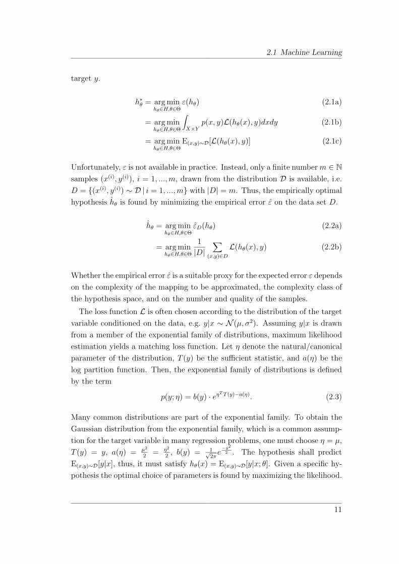
The loss function L is often chosen according to the distribution of the target
variable conditioned on the data, e.g. y|x ∼ N (µ, σ2). Assuming y|x is drawn
from a member of the exponential family of distributions, maximum likelihood
estimation yields a matching loss function. Let η denote the natural/canonical
parameter of the distribution, T (y) be the sufficient statistic, and a(η) be the
log partition function. Then, the exponential family of distributions is defined
by the term
p(y; η) = b(y) · eηTT (y)−a(η). (2.3)
Many common distributions are part of the exponential family. To obtain the
Gaussian distribution from the exponential family, which is a common assump-
tion for the target variable in many regression problems, one must choose η = µ,
T (y) = y, a(η) = µ2
2= η2
2, b(y) = 1√
2πe−y22 . The hypothesis shall predict
E(x,y)∼D[y|x], thus, it must satisfy hθ(x) = E(x,y)∼D[y|x; θ]. Given a specific hy-
pothesis the optimal choice of parameters is found by maximizing the likelihood.
11
2 Theoretical Background
θ = arg maxθ∈Θ
`(θ;D) (2.4a)
= arg maxθ∈Θ
∏
(x,y)∈D
dim(y)∏
i=1
1√2πσi
e− 1
2σ2i
(yi−[hθ(x)]i)2
(2.4b)
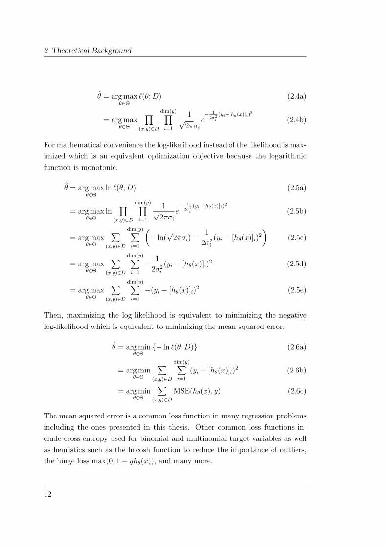
For mathematical convenience the log-likelihood instead of the likelihood is max-
imized which is an equivalent optimization objective because the logarithmic
function is monotonic.
θ = arg maxθ∈Θ
ln `(θ;D) (2.5a)
= arg maxθ∈Θ
ln∏
(x,y)∈D
dim(y)∏
i=1
1√2πσi
e− 1
2σ2i
(yi−[hθ(x)]i)2
(2.5b)
= arg maxθ∈Θ
∑
(x,y)∈D
dim(y)∑
i=1
Ç− ln(
√2πσi)−
1
2σ2i
(yi − [hθ(x)]i)2
å(2.5c)
= arg maxθ∈Θ
∑
(x,y)∈D
dim(y)∑
i=1
− 1
2σ2i
(yi − [hθ(x)]i)2 (2.5d)
= arg maxθ∈Θ
∑
(x,y)∈D
dim(y)∑
i=1
−(yi − [hθ(x)]i)2 (2.5e)
Then, maximizing the log-likelihood is equivalent to minimizing the negative
log-likelihood which is equivalent to minimizing the mean squared error.
θ = arg minθ∈Θ
− ln `(θ;D) (2.6a)
= arg minθ∈Θ
∑
(x,y)∈D
dim(y)∑
i=1
(yi − [hθ(x)]i)2 (2.6b)
= arg minθ∈Θ
∑
(x,y)∈DMSE(hθ(x), y) (2.6c)
The mean squared error is a common loss function in many regression problems
including the ones presented in this thesis. Other common loss functions in-
clude cross-entropy used for binomial and multinomial target variables as well
as heuristics such as the ln cosh function to reduce the importance of outliers,
the hinge loss max(0, 1− yhθ(x)), and many more.
12
2.2 Knowledge Transfer
2.2 Knowledge Transfer
Knowledge transfer denotes the process of using previously gained knowledge
from related tasks to improve the ability of learning a new task compared to
learning the task in isolation. The question of how to share or transfer knowledge
among multiple learning tasks dates back at least two decades.
Caruana (1993) suggested that learning multiple tasks simultaneously may
yield better generalization compared to learning multiple individual tasks sepa-
rately. He considered multiple related learning tasks to be sources of inductive
bias with mutual benefit to each other. Caruana focused on neural networks
which model multiple tasks by sharing the hidden layer in a three-layer network.
Thrun (1996) introduced the lifelong learning framework in which he derived
inspiration from human learning behavior. While a classical perspective on
learning theory is concerned with finding the optimal hypothesis that describes a
set of observed data of a particular task within a given hypothesis space, humans
follow a different learning paradigm where prior knowledge from a vast amount of
experience of related learning tasks is utilized. Thrun illustrates this perspective
with an intuitive example: “[...] when learning to drive a car, years of learning
experience with basic motor skills, typical traffic patterns, logical reasoning,
language and much more precede and influence this learning task. The transfer
of knowledge across learning tasks seems to play an essential role for generalizing
accurately, particularly when training data is scarce”. Figure 2.1 illustrates the
difference between classical machine learning and transfer learning.
Significant research has been conducted since to explore methods allowing to
transfer knowledge in various ways across domains and tasks, typically to alle-
viate the lack of labeled data in a target domain by exploiting prior knowledge
from one or multiple relevant source domain(s)/task(s). Three major survey
papers have been published in recent years that provide excellent overviews of
the field. Taylor & Stone (2009) and Torrey & Shavlik (2009) focus on trans-
fer learning in the context of reinforcement learning. Reinforcement learning
is concerned with training an agent to act optimally in a given environment
with respect to a particular task. Each action, that the agent invokes, returns
a reward to the agent. The agent’s goal is to accumulate as much reward as
possible over time which, in turn, implies a well-behaved agent with respect to
the underlying task. While this thesis is not concerned with control tasks, some
13

2 Theoretical Background
Data Data · · · Data
LearningAlgorithm
LearningAlgorithm
· · · LearningAlgorithm
Model Model · · · Model
Task #1 Task #2 Task #N
(a) Classical machine learning
Data Data · · · Data
KnowledgeLearningAlgorithm
Model
Task #1 Task #2 Task #N
(b) Transfer learning
Figure 2.1: Comparison of classical machine learning vs. transfer learning. The
illustration is adapted from Pan & Yang (2010).
of the aspects discussed in the papers are closely related to transfer learning
in the context of modeling dynamical systems. Pan & Yang (2010) provide
a more general perspective on the topic, formalize the problem of knowledge
transfer across domains and tasks, identify various transfer learning settings,
their applicability in different situations and under different constraints, as well
as approaches how to achieve knowledge transfer, and depict which approach is
viable or compatible with each learning setting.
2.2.1 Formal Definition
A learning problem consists of a domain D = (X,P ), where X is an input space
and P a probability measure which gives the marginal probability P (x) of each
example input x ∈ X, and a learning task T = (Y, h), where Y is a target space
and h : X → Y is the hypothesis that models P (y|x), y ∈ Y , which is learned
from the training data D = (x(i), y(i)) ∼ D | i = 1, ...,m. In a transfer learning
scenario, there are source domains DS,i and learning tasks TS,i, i ∈ N, and there
is a target domain DT and a learning task TT . Given this scenario, a formal
definition of transfer learning, which was adapted from Pan & Yang (2010), is
provided as follows.
14
2.2 Knowledge Transfer
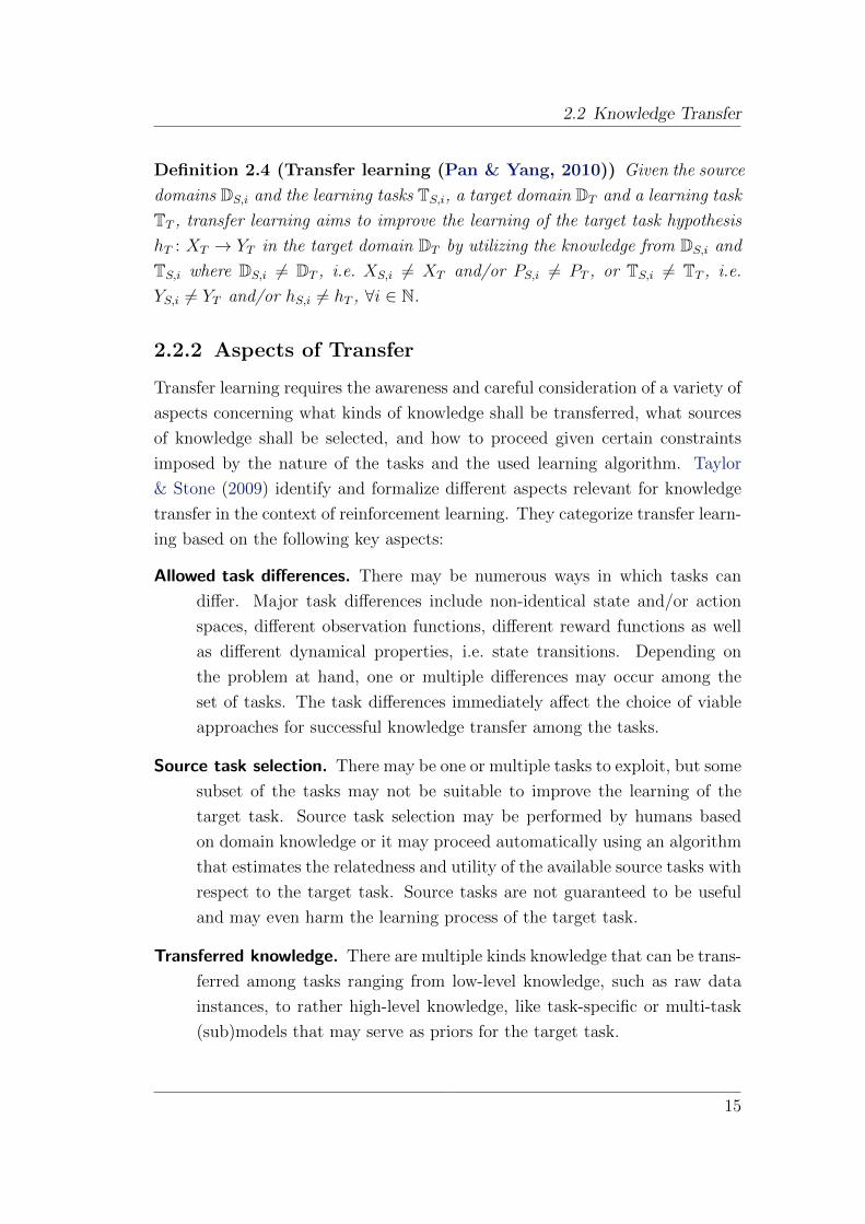
Definition 2.4 (Transfer learning (Pan & Yang, 2010)) Given the source
domains DS,i and the learning tasks TS,i, a target domain DT and a learning task
TT , transfer learning aims to improve the learning of the target task hypothesis
hT : XT → YT in the target domain DT by utilizing the knowledge from DS,i and
TS,i where DS,i 6= DT , i.e. XS,i 6= XT and/or PS,i 6= PT , or TS,i 6= TT , i.e.
YS,i 6= YT and/or hS,i 6= hT , ∀i ∈ N.
2.2.2 Aspects of Transfer
Transfer learning requires the awareness and careful consideration of a variety of
aspects concerning what kinds of knowledge shall be transferred, what sources
of knowledge shall be selected, and how to proceed given certain constraints
imposed by the nature of the tasks and the used learning algorithm. Taylor
& Stone (2009) identify and formalize different aspects relevant for knowledge
transfer in the context of reinforcement learning. They categorize transfer learn-
ing based on the following key aspects:
Allowed task differences. There may be numerous ways in which tasks can
differ. Major task differences include non-identical state and/or action
spaces, different observation functions, different reward functions as well
as different dynamical properties, i.e. state transitions. Depending on
the problem at hand, one or multiple differences may occur among the
set of tasks. The task differences immediately affect the choice of viable
approaches for successful knowledge transfer among the tasks.
Source task selection. There may be one or multiple tasks to exploit, but some
subset of the tasks may not be suitable to improve the learning of the
target task. Source task selection may be performed by humans based
on domain knowledge or it may proceed automatically using an algorithm
that estimates the relatedness and utility of the available source tasks with
respect to the target task. Source tasks are not guaranteed to be useful
and may even harm the learning process of the target task.
Transferred knowledge. There are multiple kinds knowledge that can be trans-
ferred among tasks ranging from low-level knowledge, such as raw data
instances, to rather high-level knowledge, like task-specific or multi-task
(sub)models that may serve as priors for the target task.
15
2 Theoretical Background
Task mappings. Tasks may have different state and/or action spaces and/or
observation functions. For instance, the state variables may only be par-
tially observable and different tasks may only be able to observe non-
identical subsets of the state variables. It is also conceivable that multiple
tasks observe the same subset of the state variables, but the variables are
observed differently, e.g. sensors may be measuring the same quantities
in different units. In such situations, it is desirable to map the available
information to a unified representation which may be achievable either
manually using domain knowledge or automatically from data.
Allowed learners. The choice of the learning algorithm may constrain the com-
patible scenarios. For instance, a partially observable system may require
a method to reconstruct the full state while it is readily available given a
fully observable system.
2.2.3 Settings
While traditional machine learning assumes identical source and target do-
mains/tasks, the domains and/or tasks may differ in a transfer learning setting.
Pan & Yang (2010) distinguish three transfer learning settings which account
for different task relations between the source and target domains/tasks.
Inductive transfer learning. Inductive transfer learning utilizes few labeled data
from the target domain to induce the target function of interest by trans-
ferring knowledge typically from labeled data in the source domain. When
large amounts of labeled data are available in the source domain, induc-
tive transfer learning is similar to multi-task learning except that it is
only concerned with improving the target task performance by utilizing
information from the source task.
Transductive transfer learning. Transductive transfer learning assumes iden-
tical source and target tasks but different domains. Further, while there
are labeled data available in the source domain, only unlabeled data are
available in the target domain. Transductive transfer can be divided into
two cases where (i) the source and target domains are actually different,
and (ii) the feature spaces of the source and target domains are equal, but
the marginal probability distributions are different.
16
2.2 Knowledge Transfer
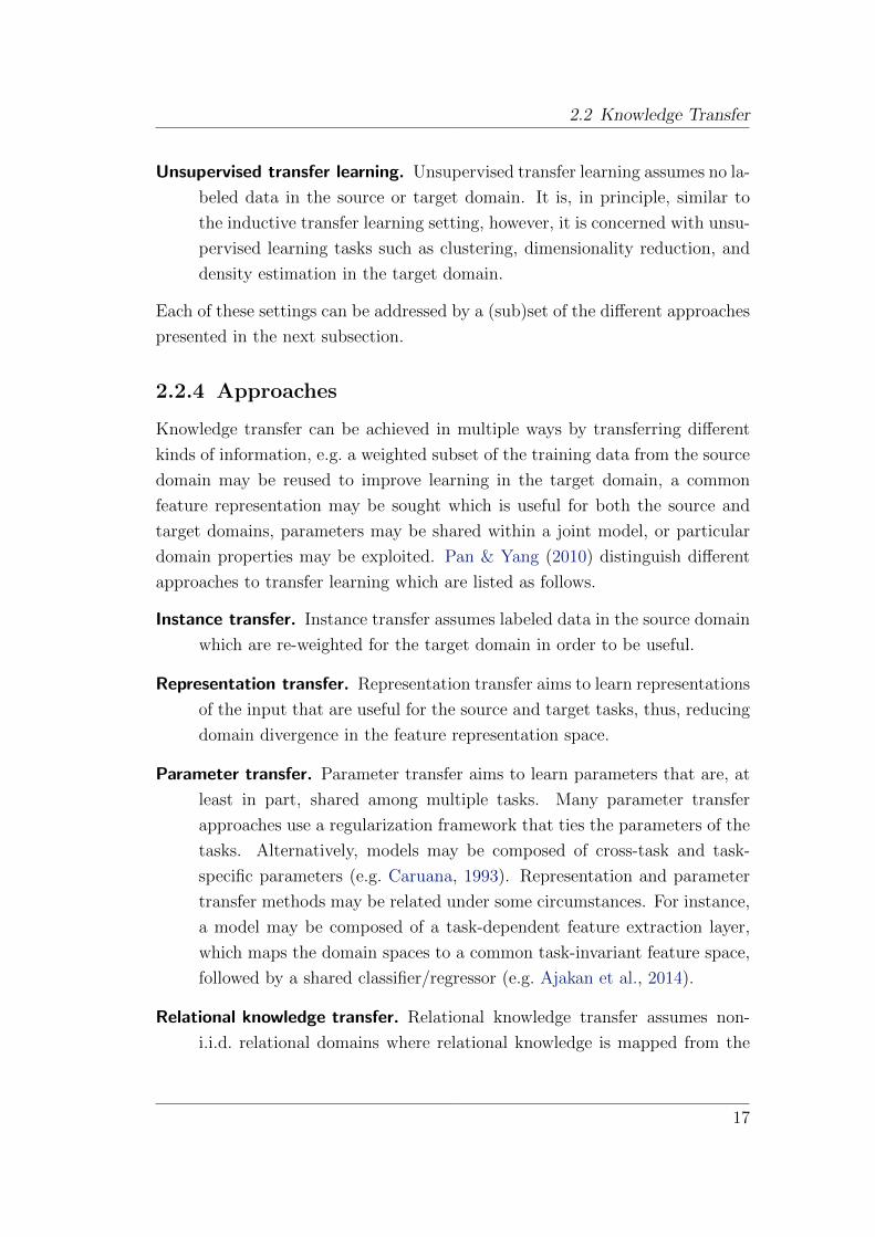
Unsupervised transfer learning. Unsupervised transfer learning assumes no la-
beled data in the source or target domain. It is, in principle, similar to
the inductive transfer learning setting, however, it is concerned with unsu-
pervised learning tasks such as clustering, dimensionality reduction, and
density estimation in the target domain.
Each of these settings can be addressed by a (sub)set of the different approaches
presented in the next subsection.
2.2.4 Approaches
Knowledge transfer can be achieved in multiple ways by transferring different
kinds of information, e.g. a weighted subset of the training data from the source
domain may be reused to improve learning in the target domain, a common
feature representation may be sought which is useful for both the source and
target domains, parameters may be shared within a joint model, or particular
domain properties may be exploited. Pan & Yang (2010) distinguish different
approaches to transfer learning which are listed as follows.
Instance transfer. Instance transfer assumes labeled data in the source domain
which are re-weighted for the target domain in order to be useful.
Representation transfer. Representation transfer aims to learn representations
of the input that are useful for the source and target tasks, thus, reducing
domain divergence in the feature representation space.
Parameter transfer. Parameter transfer aims to learn parameters that are, at
least in part, shared among multiple tasks. Many parameter transfer
approaches use a regularization framework that ties the parameters of the
tasks. Alternatively, models may be composed of cross-task and task-
specific parameters (e.g. Caruana, 1993). Representation and parameter
transfer methods may be related under some circumstances. For instance,
a model may be composed of a task-dependent feature extraction layer,
which maps the domain spaces to a common task-invariant feature space,
followed by a shared classifier/regressor (e.g. Ajakan et al., 2014).
Relational knowledge transfer. Relational knowledge transfer assumes non-
i.i.d. relational domains where relational knowledge is mapped from the
17
2 Theoretical Background
source domain(s) to the target domain.
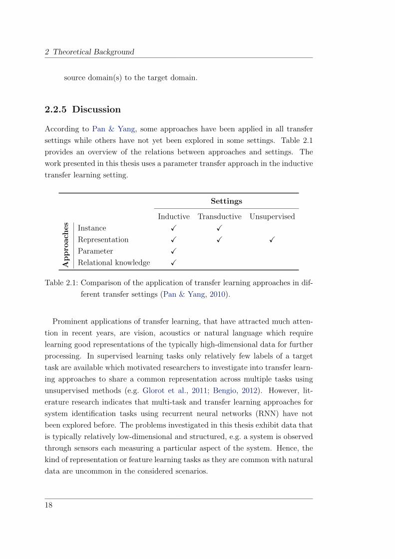
2.2.5 Discussion
According to Pan & Yang, some approaches have been applied in all transfer
settings while others have not yet been explored in some settings. Table 2.1
provides an overview of the relations between approaches and settings. The
work presented in this thesis uses a parameter transfer approach in the inductive
transfer learning setting.
Settings
Inductive Transductive Unsupervised
Ap
pro
ach
es
Instance X X
Representation X X X
Parameter X
Relational knowledge X
Table 2.1: Comparison of the application of transfer learning approaches in dif-
ferent transfer settings (Pan & Yang, 2010).
Prominent applications of transfer learning, that have attracted much atten-
tion in recent years, are vision, acoustics or natural language which require
learning good representations of the typically high-dimensional data for further
processing. In supervised learning tasks only relatively few labels of a target
task are available which motivated researchers to investigate into transfer learn-
ing approaches to share a common representation across multiple tasks using
unsupervised methods (e.g. Glorot et al., 2011; Bengio, 2012). However, lit-
erature research indicates that multi-task and transfer learning approaches for
system identification tasks using recurrent neural networks (RNN) have not
been explored before. The problems investigated in this thesis exhibit data that
is typically relatively low-dimensional and structured, e.g. a system is observed
through sensors each measuring a particular aspect of the system. Hence, the
kind of representation or feature learning tasks as they are common with natural
data are uncommon in the considered scenarios.
18
2.3 Neural Networks
2.3 Neural Networks
Neural networks (e.g. Krose & van der Smagt, 1994) are biologically inspired
nonlinear parametric models. They consist of neurons, which are represented
as nodes in the network, and synapses, which are represented as connections or
adaptive weights between nodes. The value of a weight determines the connec-
tion strength between two neurons. In order to identify the relationship between
the presented inputs and targets the weights are adapted, or learned, such that
the expected error of the model is minimized. Neural networks are highly con-
figurable models which allows the designer to incorporate domain knowledge
into the architecture. Among the vast space of possibilities several key architec-
tures have emerged. The following subsections will introduce the perceptron,
multi-layer perceptron, and the Elman recurrent neural network architecture.
2.3.1 Perceptron
The perceptron is the most basic type of neural network (Rosenblatt, 1958;
Minsky & Papert, 1988). It implements a simple artificial neuron with a thresh-
old function whose incoming weights are adaptive and learned from data. As
opposed to the logistic regression model, whose output is a weighted linear com-
bination of the inputs followed by a smooth nonlinear sigmoid function yielding
values in the range ]0, 1[, the perceptron’s output is a weighted linear combina-
tion of the inputs forced to the binary values 0, 1 by means of a threshold.
Mathematically, the perceptron hypothesis is defined by the equation
hθ(x) =
1 if wTx+ b > 0
0 else(2.7)
where x ∈ Rn is the input vector, w ∈ Rn is the weights vector, and b ∈ R is
a bias weight, thus, θ = w, b. Figure 2.2 illustrates the perceptron model.
After the weights are initialized randomly or with zero values they are adapted
to minimize the empirical error between the predicted output y = hθ(x) and the
target y ∈ 0, 1 using the perceptron learning rule.
w ← w + α(y − y) • x (2.8a)
b← b+ α(y − y) (2.8b)
19

2 Theoretical Background
x1 x2 . . . xn1
y
w 1
w2
wnb
Figure 2.2: Perceptron
The bold bullet “•” denotes the pointwise vector product and α > 0 is the
learning rate. The perceptron learning rule is similar to the gradient descent
learning rule, which is covered in Section 2.4.1.
2.3.2 Multi-Layer Perceptron
The multi-layer perceptron (MLP) is an extension of the perceptron consisting of
multiple layers of artificial neurons equipped with nonlinear activation functions.
In contrast to the perceptron model the MLP is able to extract increasingly
abstract representations of the inputs by stacking multiple layers of hidden
neurons on top of each other. It has been proven that the MLP is a universal
function approximator, i.e. it can approximate any continuous function on a
compact domain with arbitrary accuracy, provided it has at least a single hidden
layer with a sufficient number of neurons (Cybenko, 1989; Hornik et al., 1989;
Hornik, 1991; Haykin, 1998).
To formalize the model, let ni denote the dimensionality of layer i in an MLP.
Further, let W (i) ∈ Rni×ni+1 be the weight matrix from layer i to layer i + 1,
b(i) ∈ Rni+1 be the bias weight vector of layer i + 1, and φ(i) : R → R be an
elementwise nonlinear activation function applied to layer i. Typical activation
20

2.3 Neural Networks
functions are
tanh(x) :=ex − e−xex + e−x
(2.9)
logistic(x) :=1
1 + e−x(2.10)
relu(x) :=
x if x > 0
0 else. (2.11)
Figure 2.3 depicts the activation functions. An MLP with l layers (including
−3 −2 −1 1 2 3
−1
1
x
φ(x)
(a) φ(x) = tanh(x)
−3 −2 −1 1 2 3
0.5
1
x
φ(x)
(b) φ(x) = logistic(x)
−1 −0.5 0.5 1
0.5
1
x
φ(x)
(c) φ(x) = relu(x)
Figure 2.3: Activation functions
the input and output layer) is described by the following equations.
z(1) = x (2.12a)
a(2) = W (1)z(1) + b(1) (2.12b)
z(2) = φ(2)(a(2)) (2.12c)
...
a(l) = W (l−1)z(l−1) + b(l−1) (2.12d)
z(l) = φ(l)(a(l)) (2.12e)
y = z(l) (2.12f)
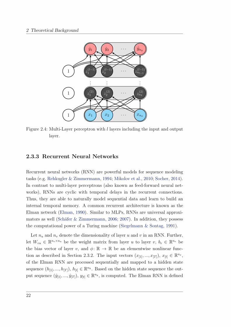
Figure 2.4 depicts the MLP architecture.
Let θ := W (1), b(1), ...,W (l−1), b(l−1) be the parameters of the MLP of equa-
tions (2.12a) to (2.12f). Then, the optimal parameters θ∗ of the model are found
by minimizing the error between the model output and the data (x, y) ∈ D given
the inputs x and the targets y.
θ∗ = arg minθ
1
|D|∑
(x,y)∈DL(y, y) (2.13)
21
2 Theoretical Background
1 x1 x2 . . . xnx
1 z(2)1 z
(2)2
. . . z(2)n2
......
...
1 z(l−1)1 z
(l−1)2
. . . z(l−1)nl−1
y1 y2 . . . yny
Figure 2.4: Multi-Layer perceptron with l layers including the input and output
layer.
2.3.3 Recurrent Neural Networks
Recurrent neural networks (RNN) are powerful models for sequence modeling
tasks (e.g. Rehkugler & Zimmermann, 1994; Mikolov et al., 2010; Socher, 2014).
In contrast to multi-layer perceptrons (also known as feed-forward neural net-
works), RNNs are cyclic with temporal delays in the recurrent connections.
Thus, they are able to naturally model sequential data and learn to build an
internal temporal memory. A common recurrent architecture is known as the
Elman network (Elman, 1990). Similar to MLPs, RNNs are universal approxi-
mators as well (Schafer & Zimmermann, 2006; 2007). In addition, they possess
the computational power of a Turing machine (Siegelmann & Sontag, 1991).
Let nu and nv denote the dimensionality of layer u and v in an RNN. Further,
let Wvu ∈ Rnv×nu be the weight matrix from layer u to layer v, bv ∈ Rnv be
the bias vector of layer v, and φ : R → R be an elementwise nonlinear func-
tion as described in Section 2.3.2. The input vectors (x[1], ..., x[T ]), x[t] ∈ Rnx ,
of the Elman RNN are processed sequentially and mapped to a hidden state
sequence (h[1], ..., h[T ]), h[t] ∈ Rnh . Based on the hidden state sequence the out-
put sequence (y[1], ..., y[T ]), y[t] ∈ Rny , is computed. The Elman RNN is defined
22

2.3 Neural Networks
recursively for t = 1, ..., T by the following equations
h[0] = hinit (2.14a)
h[t] = φh(Whxx[t] +Whhh[t−1] + bh) (2.14b)
y[t] = φy(Wyhh[t] + by) (2.14c)
with some initial state hinit ∈ Rnh . It is common to either set hinit = 0 or treat
it as an additional parameter vector to be learned. Figure 2.5 illustrates the
Elman RNN architecture using recurrent connections in the hidden layer. An
1 x[t]1 x[t]2 . . . x[t]nx
1 h[t]1 h[t]2 . . . h[t]nh
y[t]1 y[t]2 . . . y[t]ny
Figure 2.5: Elman RNN
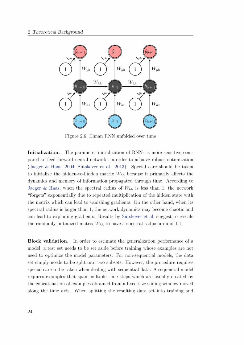
alternative visualization of RNN architectures draws the network unfolded in
time for a finite number of time steps. To improve readability only clusters of
neurons are drawn instead of each individual one. An arrow then represents a
full connection between two clusters of neurons, i.e. each neuron in the source
cluster is connected with each neuron in the destination cluster. Figure 2.6
depicts the network architecture unfolded for three time steps.
Let θ := Whx,Whh, bh,Wyh, by be the RNN parameters of equations (2.14a)
to (2.14c). Then, the optimal parameters θ∗ of the model are found by fitting
the model to the data, given the inputs x[t] and the targets y[t], over a fixed
number of T time steps.
θ∗ = arg minθ
1
|D| · T∑
(x[1],y[1]...,x[T ],y[T ])∈D
T∑
t=1
L(y[t], y[t]) (2.15)
23
2 Theoretical Background
1 1 1
x[t−1] x[t] x[t+1]
1 1 1
h[t−1] h[t] h[t+1]
Whx Whx Whx
b h b h b h
Whh Whh
y[t−1] y[t] y[t+1]
Wyh Wyh Wyhb y b y b y
Figure 2.6: Elman RNN unfolded over time
Initialization. The parameter initialization of RNNs is more sensitive com-
pared to feed-forward neural networks in order to achieve robust optimization
(Jaeger & Haas, 2004; Sutskever et al., 2013). Special care should be taken
to initialize the hidden-to-hidden matrix Whh because it primarily affects the
dynamics and memory of information propagated through time. According to
Jaeger & Haas, when the spectral radius of Whh is less than 1, the network
“forgets” exponentially due to repeated multiplication of the hidden state with
the matrix which can lead to vanishing gradients. On the other hand, when its
spectral radius is larger than 1, the network dynamics may become chaotic and
can lead to exploding gradients. Results by Sutskever et al. suggest to rescale
the randomly initialized matrix Whh to have a spectral radius around 1.1.
Block validation. In order to estimate the generalization performance of a
model, a test set needs to be set aside before training whose examples are not
used to optimize the model parameters. For non-sequential models, the data
set simply needs to be split into two subsets. However, the procedure requires
special care to be taken when dealing with sequential data. A sequential model
requires examples that span multiple time steps which are usually created by
the concatenation of examples obtained from a fixed-size sliding window moved
along the time axis. When splitting the resulting data set into training and
24
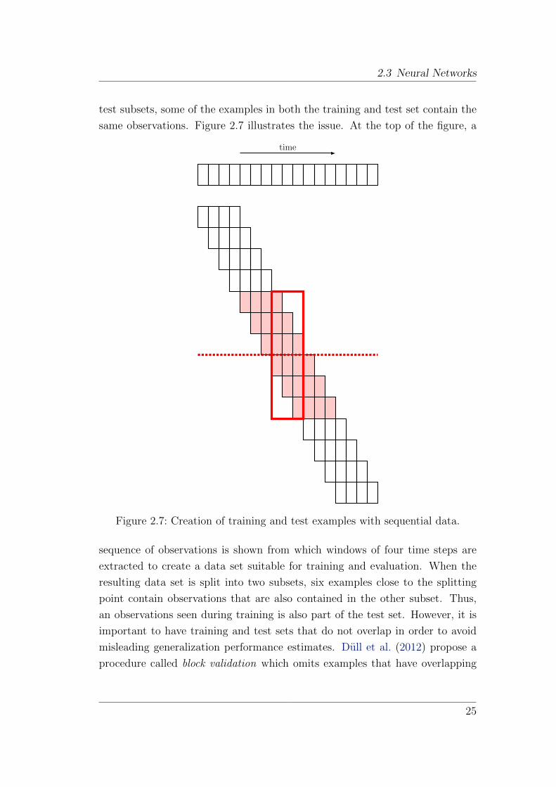
2.3 Neural Networks
test subsets, some of the examples in both the training and test set contain the
same observations. Figure 2.7 illustrates the issue. At the top of the figure, a
time
Figure 2.7: Creation of training and test examples with sequential data.
sequence of observations is shown from which windows of four time steps are
extracted to create a data set suitable for training and evaluation. When the
resulting data set is split into two subsets, six examples close to the splitting
point contain observations that are also contained in the other subset. Thus,
an observations seen during training is also part of the test set. However, it is
important to have training and test sets that do not overlap in order to avoid
misleading generalization performance estimates. Dull et al. (2012) propose a
procedure called block validation which omits examples that have overlapping
25

2 Theoretical Background
observations in the training and test set. Further, they suggest to select multiple
blocks at random instead of splitting the data set into two contiguous chunks.
2.4 Learning & Optimization
Learning the parameters of a neural network is typically performed using first-
order optimization techniques, such as gradient descent or variants thereof. To
do so, it is necessary to compute the partial derivatives of the error function with
respect to the parameters. While, in general, this simply requires multivariate
calculus and, in particular, means applying the chain rule repeatedly, it is not
immediately obvious that computing the partial derivatives naıvely results in
redundant computations. However, combining the rules of calculus and dynamic
programming yields an algorithm called backpropagation which is an efficient
way of obtaining the partial derivatives.
The following subsections introduce the backpropagation algorithm and Hessian-
Free optimization—a second-order optimization method that has been shown to
be a powerful technique to learn the parameters of recurrent neural networks.
Further, complex models, such as neural networks, are prone to overfitting, i.e.
memorizing input patterns rather than inferring the underlying structure from
examples. Several techniques to reduce this phenomenon have emerged some of
which are revised in this section.
2.4.1 Backpropagation
The backpropagation algorithm (Rumelhart, 1986; Rumelhart et al., 1988) is
an efficient method to compute the partial derivatives of an error function with
respect to its parameters. In essence, it combines multivariate calculus with dy-
namic programming in order to reuse previously computed parts of the gradient.
A three-layer feed-forward network as introduced in Section 2.3.2 will serve as an
example to derive the algorithm and discuss its importance for efficient learning.
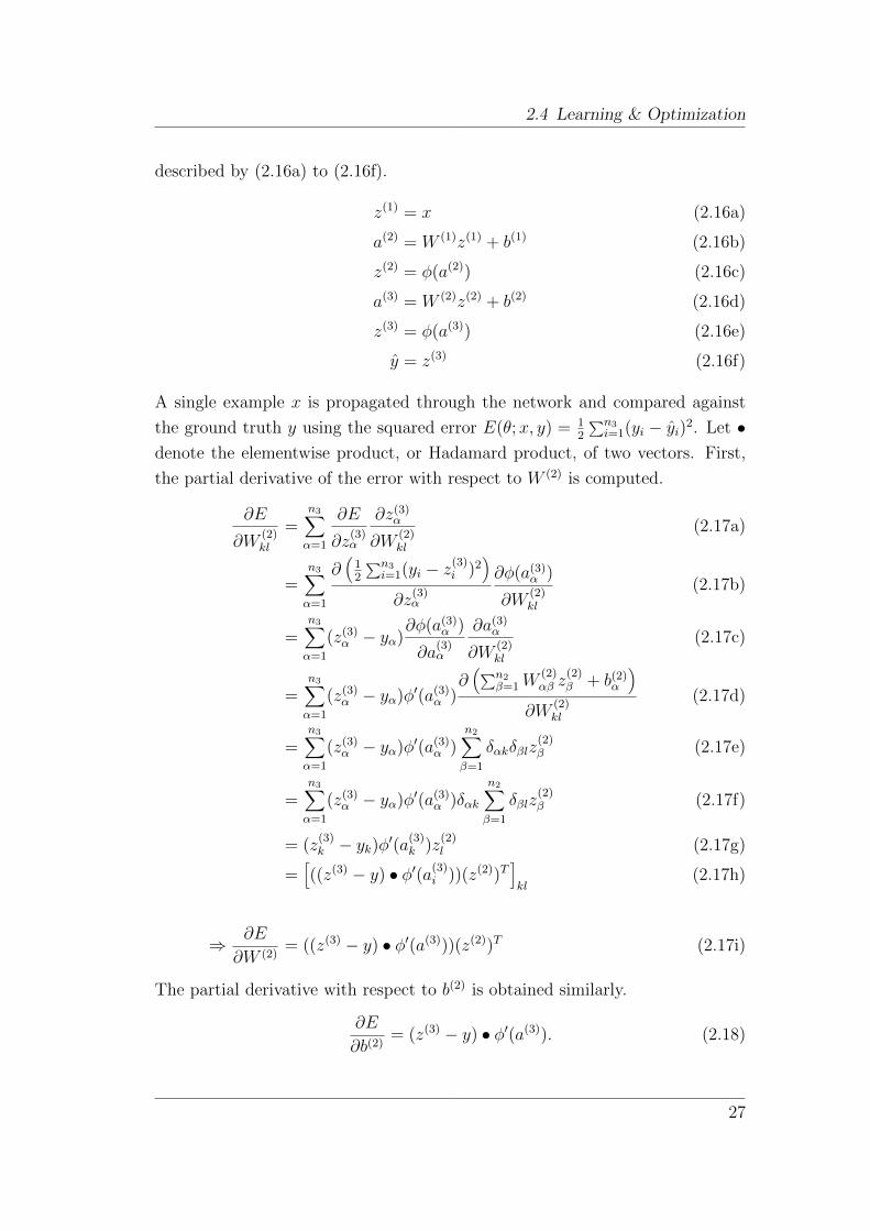
Let θ = W (1), b(1),W (2), b(2) be the parameters of a three-layer perceptron
26
2.4 Learning & Optimization
described by (2.16a) to (2.16f).
z(1) = x (2.16a)
a(2) = W (1)z(1) + b(1) (2.16b)
z(2) = φ(a(2)) (2.16c)
a(3) = W (2)z(2) + b(2) (2.16d)
z(3) = φ(a(3)) (2.16e)
y = z(3) (2.16f)
A single example x is propagated through the network and compared against
the ground truth y using the squared error E(θ;x, y) = 12
∑n3i=1(yi − yi)2. Let •
denote the elementwise product, or Hadamard product, of two vectors. First,
the partial derivative of the error with respect to W (2) is computed.
∂E
∂W(2)kl
=n3∑
α=1
∂E
∂z(3)α
∂z(3)α
∂W(2)kl
(2.17a)
=n3∑
α=1
∂(
12
∑n3i=1(yi − z(3)
i )2)
∂z(3)α
∂φ(a(3)α )
∂W(2)kl
(2.17b)
=n3∑
α=1
(z(3)α − yα)
∂φ(a(3)α )
∂a(3)α
∂a(3)α
∂W(2)kl
(2.17c)
=n3∑
α=1
(z(3)α − yα)φ′(a(3)
α )∂(∑n2
β=1W(2)αβ z
(2)β + b(2)
α
)
∂W(2)kl
(2.17d)
=n3∑
α=1
(z(3)α − yα)φ′(a(3)
α )n2∑
β=1
δαkδβlz(2)β (2.17e)
=n3∑
α=1
(z(3)α − yα)φ′(a(3)
α )δαkn2∑
β=1
δβlz(2)β (2.17f)
= (z(3)k − yk)φ′(a(3)
k )z(2)l (2.17g)
=[((z(3) − y) • φ′(a(3)
i ))(z(2))T]kl
(2.17h)
⇒ ∂E
∂W (2)= ((z(3) − y) • φ′(a(3)))(z(2))T (2.17i)
The partial derivative with respect to b(2) is obtained similarly.
∂E
∂b(2)= (z(3) − y) • φ′(a(3)). (2.18)
27
2 Theoretical Background
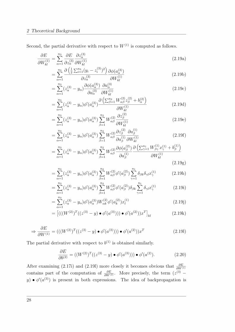
Second, the partial derivative with respect to W (1) is computed as follows.
∂E
∂W(1)kl
=n3∑
α=1
∂E
∂z(3)α
∂z(3)α
∂W(1)kl
(2.19a)
=n3∑
α=1
∂(
12
∑n3i=1(yi − z(3)
i )2)
∂z(3)α
∂φ(a(3)α )
∂W(1)kl
(2.19b)
=n3∑
α=1
(z(3)α − yα)
∂φ(a(3)α )
∂a(3)α
∂a(3)α
∂W(1)kl
(2.19c)
=n3∑
α=1
(z(3)α − yα)φ′(a(3)
α )∂(∑n2
β=1W(2)αβ z
(2)β + b(2)
α
)
∂W(1)kl
(2.19d)
=n3∑
α=1
(z(3)α − yα)φ′(a(3)
α )n2∑
β=1
W(2)αβ
∂z(2)β
∂W(1)kl
(2.19e)
=n3∑
α=1
(z(3)α − yα)φ′(a(3)
α )n2∑
β=1
W(2)αβ
∂z(2)β
∂a(1)β
∂a(1)β
∂W(1)kl
(2.19f)
=n3∑
α=1
(z(3)α − yα)φ′(a(3)
α )n2∑
β=1
W(2)αβ
∂φ(a(2)β )
∂a(1)β
∂(∑n1
γ=1 W(1)βγ x
(1)γ + b
(1)β
)
∂W(1)kl
(2.19g)
=n3∑
α=1
(z(3)α − yα)φ′(a(3)
α )n2∑
β=1
W(2)αβ φ
′(a(2)β )
n1∑
γ=1
δβkδγlx(1)γ (2.19h)
=n3∑
α=1
(z(3)α − yα)φ′(a(3)
α )n2∑
β=1
W(2)αβ φ
′(a(2)β )δβk
n1∑
γ=1
δγlx(1)γ (2.19i)
=n3∑
α=1
(z(3)α − yα)φ′(a(3)
α )W(2)αk φ
′(a(2)k )x
(1)l (2.19j)
=î(((W (2))T ((z(3) − y) • φ′(a(3)))) • φ′(a(2)))xT
ókl
(2.19k)
⇒ ∂E
∂W (1)= (((W (2))T ((z(3) − y) • φ′(a(3)))) • φ′(a(2)))xT (2.19l)
The partial derivative with respect to b(1) is obtained similarly.
∂E
∂b(2)= ((W (2))T ((z(3) − y) • φ′(a(3)))) • φ′(a(2)). (2.20)
After examining (2.17i) and (2.19l) more closely it becomes obvious that ∂E∂W (1)
contains part of the computation of ∂E∂W (2) . More precisely, the term (z(3) −
y) • φ′(a(3)) is present in both expressions. The idea of backpropagation is
28
2.4 Learning & Optimization
to reuse parts of the derivative computed in higher layers, i.e. layers close to
the output of the network, in order to compute the derivatives of lower layers.
Therefore, parts of the derivatives of the higher layers are tabulated and looked
up instead of recomputed by the lower layer derivatives. Then, computing the
derivatives looks similar to the forward propagation shown in (2.16a) to (2.16f)
but performed in reverse direction, hence, the term backpropagation. First, the
errors are propagated backwards yielding the following local error message, or
so-called delta messages.
δ(3) = (z(3) − y) • φ(a(3)) (2.21a)
δ(2) = ((W (2))T δ(2)) • φ(a(2)) (2.21b)
Second, once the delta messages are computed the partial derivatives are easily
obtained as follows.
∂E
∂W (2)= δ(2)(z(2))T (2.22a)
∂E
∂b(2)= δ(3) (2.22b)
∂E
∂W (1)= δ(2)(z(1))T = δ(2)xT (2.22c)
∂E
∂b(1)= δ(2) (2.22d)
While this example demonstrates the backpropagation algorithm for a three-
layer feed-forward network, it generalizes for an arbitrary number of layers as
well as for recurrent architectures, whose extension is called backpropagation
through time (BPTT), and for arbitrary directed acyclic computation graphs,
which is called backpropagation through structure (BTS). Using the first deriva-
tives computed by backpropagation, the model parameters are adapted to min-
imize the error function. Often, simple first-order optimization methods, such
as (stochastic) gradient descent or variants thereof, are used. However, it has
been observed that learning the parameters of recurrent neural networks with
first-order optimization methods may be troublesome due to the so-called van-
ishing and exploding gradient problem (Hochreiter, 1991; Bengio et al., 1994;
Hochreiter et al., 2001). The next subsection introduces a second-order opti-
mization method that has been shown to overcome these difficulties and which
29
2 Theoretical Background
is capable of handling even a large number of parameters—a common property
of neural network models.
2.4.2 Hessian-Free Optimization
Hessian-Free optimization (Martens, 2010; Martens & Sutskever, 2011; 2012)
is an approximate Newton method suitable for training models with a large
number of parameters, e.g. neural networks. Especially in deep learning, where
many layers of abstraction are used to extract complex features from the input
data, slow and ineffective learning has been observed. Non-random initialization
through layerwise pre-training using Restricted Boltzmann Machines (Hinton &
Salakhutdinov, 2006) and shallow autoencoders (Bengio et al., 2007) has been
found to give significant improvements. However, these approaches are designed
for deep feed-forward neural networks which is a rather strong limitation given
the flexibility entailed by general neural networks. Since Hessian-Free optimiza-
tion is a general optimization method, it imposes fewer constraints on the model.
Martens & Sutskever demonstrated that this approach is well suited for non-
convex neural network objective functions that had been difficult to optimize
including deep feedforward and recurrent neural networks.
In contrast to first-order optimization methods, Hessian-Free optimization
constructs a local quadratic approximation of the objective function at the cur-
rent location in the parameter space, thus, utilizing curvature information in
addition to the gradient. Let B(θ(k−1)) be the curvature matrix, e.g. the Hessian
H(θ(k−1)) of the objective f(θ) := ε(hθ) at θ(k−1) where hθ is the parameterized
hypothesis as described in Section 2.1. Then, a local quadratic approximation
M (k−1) of f at θ(k−1) is formed using the Taylor expansion up to degree two.
M (k−1)(∆θ) = f(θ(k−1)) +∇f(θ(k−1))T∆θ +1
2(∆θ)TB(θ(k−1))∆θ (2.23)
Using M (k−1), the parameters are updated according to the following rule
θ(k) = θ(k−1) + α(k)
Çarg min
∆θ∈ΘM (k−1)(∆θ)
å, (2.24)
provided that the minimizer exists, with the step length α(k) ∈ [0, 1] typically
chosen using line-search (Nocedal & Wright, 2006). Martens & Sutskever pro-
pose to use the backtracking line-search starting with α(k) = 1.
30

2.4 Learning & Optimization
The minimizer of M (k−1) exists if B(θ(k−1)) is positive definite and is found by
the Newton step (∆θ(k))∗ = θ(k−1)−B−1(θ(k−1))∇f(θ(k−1)). There are a number
of problems with the standard Newton method when used to optimize neural
network objective functions.
1. First, B(θ(k−1)), e.g. the Hessian matrix, is prohibitively large for models
with many parameters such as neural networks. It requires computing
and storing the number of parameters squared. Architectures nowadays
may easily consist of millions of parameters yielding a matrix with 1012 or
more entries.
2. Second, even if B(θ(k−1)) could be computed and stored, inverting it, or
equivalently solving the system of equationsB(θ(k−1))∆θ(k) = −∇f(θ(k−1)),
is impractical.
3. Third, since most neural network objectives are non-convex its Hessian is
not positive definite everywhere in the parameter space. Thus, B(θ(k−1)) =
H(θ(k−1)) may not always be invertible.
Martens & Sutskever address these obstacles as follows. In order to guarantee
semi positive definiteness of B(θ(k−1)) they use the generalized Gauss-Newton
matrix instead of the Hessian, which is an approximation of the Hessian matrix.
For details, see (Martens & Sutskever, 2012, Section 6). Since the generalized
Gauss-Newton matrix is only semi-positive definite, but inverting a matrix re-
quires strict positive definiteness, Tikhonov damping is added which raises all
eigenvalues by a small positive number λ > 0, thus, making it strictly positive
definite. Further, the generalized Gauss-Newton matrix is symmetric. Inversion
of this matrix is performed by solving the above system of equations using the
(preconditioned) conjugate gradient method (Golub & van Loan, 1996; Nocedal
& Wright, 2006) which is an iterative algorithm with desirable convergence prop-
erties. In theory, and given infinite precision arithmetic, the conjugate gradient
method is guaranteed to converge in at most |θ| iterations. However, in practice,
and despite finite precision arithmetic, it typically reaches a small residual after
many fewer than |θ| iterations. For details, please consult the above referenced
literature. Finally, computing and storing the curvature matrix can be avoided
due to the work of Pearlmutter (1994) and by observing that the conjugate
31
2 Theoretical Background
gradient method merely requires the matrix-vector product of the system ma-
trix (typically the generalized Gauss-Newton matrix) with an internal vector.
Pearlmutter proposes a computationally efficient method called the R-operator,
similar in notion to the backpropagation algorithm, which computes the product
of the Hessian with a vector exactly without explicitly forming the matrix.
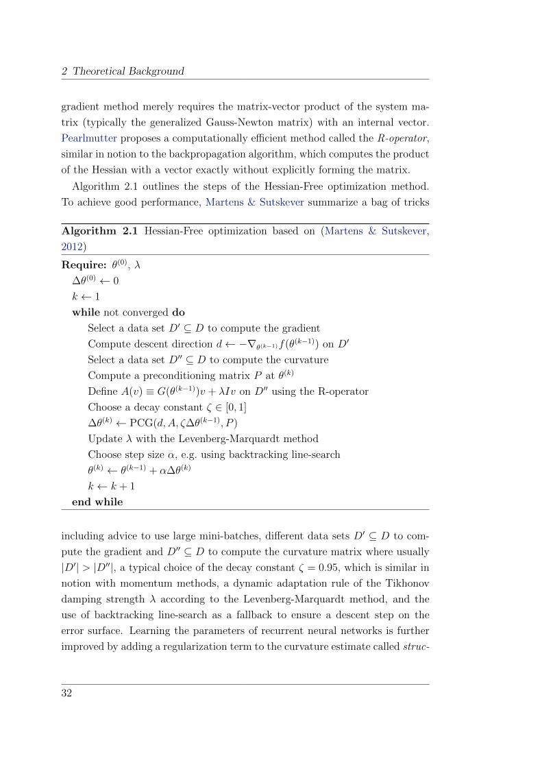
Algorithm 2.1 outlines the steps of the Hessian-Free optimization method.
To achieve good performance, Martens & Sutskever summarize a bag of tricks
Algorithm 2.1 Hessian-Free optimization based on (Martens & Sutskever,
2012)
Require: θ(0), λ
∆θ(0) ← 0
k ← 1
while not converged do
Select a data set D′ ⊆ D to compute the gradient
Compute descent direction d← −∇θ(k−1)f(θ(k−1)) on D′
Select a data set D′′ ⊆ D to compute the curvature
Compute a preconditioning matrix P at θ(k)
Define A(v) ≡ G(θ(k−1))v + λIv on D′′ using the R-operator
Choose a decay constant ζ ∈ [0, 1]
∆θ(k) ← PCG(d,A, ζ∆θ(k−1), P )
Update λ with the Levenberg-Marquardt method
Choose step size α, e.g. using backtracking line-search
θ(k) ← θ(k−1) + α∆θ(k)
k ← k + 1
end while
including advice to use large mini-batches, different data sets D′ ⊆ D to com-
pute the gradient and D′′ ⊆ D to compute the curvature matrix where usually
|D′| > |D′′|, a typical choice of the decay constant ζ = 0.95, which is similar in
notion with momentum methods, a dynamic adaptation rule of the Tikhonov
damping strength λ according to the Levenberg-Marquardt method, and the
use of backtracking line-search as a fallback to ensure a descent step on the
error surface. Learning the parameters of recurrent neural networks is further
improved by adding a regularization term to the curvature estimate called struc-
32
2.4 Learning & Optimization
tural damping (Martens & Sutskever, 2011). The intuition behind structural
damping is as follows. Adjusting the parameters of a recurrent neural network,
in particular the hidden-to-hidden matrix Whh, causes large fluctuations in the
hidden state sequence due to the recursive and highly nonlinear nature of this
model. Thus, large parameter update steps may be untrustworthy and harm-
ful to the optimization process. To avoid this issue, one could reduce the step
size α, or, similarly, use a large Tikhonov damping coefficient λ, but this alle-
viates the advantage of utilizing curvature information to make larger update
steps in the directions of low curvature. Instead, structural damping penalizes
large changes in the hidden state sequence, thus, the parameters themselves are
not regularized but rather the effect of their update with respect to the hidden
dynamics.
2.4.3 Overfitting
Overfitting is a phenomenon commonly faced in statistics and machine learning
when a model memorizes the presented data instead of identifying the underlying
structure. It typically occurs when complex models, i.e. models with many
degrees of freedom, are fitted to comparatively few examples. Consequently,
such a model has poor generalization capabilities which become apparent when
it is tested on an independent set of examples that was unseen during training.
To avoid overfitting, several techniques have emerged such as regularization,
early stopping, and ensemble learning, among others.
Regularization
Regularization is a method to reduce the effective model complexity by intro-
ducing additional information to the model typically by imposing (smoothness)
constraints on its parameters (Girosi et al., 1995). The most common techniques
in machine learning are known as L1 and L2 regularization which are added to
the objective function to be minimized. They penalize the model parameters
according to the Lp norm which, in the case of p = 1, yields sparse parameters
or, in the case of p = 2, avoids large values. Especially in the neural networks
community the L2 regularization is also known as weight decay.
Another more recently introduced and popular approach is called dropout
(e.g. Hinton et al., 2012; Srivastava et al., 2014; Bayer et al., 2014). It randomly
33

2 Theoretical Background
sets incoming neurons to zero in each training example and, thus, prevents co-
adaptation feature extractors. Alternatively, dropout can be considered a model
averaging technique where an exponential number of submodels shares the same
set of parameters.
Early Stopping
Early-stopping (e.g. Yao et al., 2007) is a different kind of regularization tech-
nique that does not rely on altering the model and/or the objective function.
However, the underlying idea is similar to that of L2 regularization which as-
sumes that smaller parameter values are preferable. Early-stopping monitors an
estimate of the generalization error on a validation set whose examples are not
used to update the model parameters. As long as the error on the validation set
improves sufficiently, training proceeds. Else, the training procedure is stopped
following the assumption that the model is starting to memorize rather than
generalize.
Ensemble Learning
Ensemble learning is a technique to utilize multiple models of a given learn-
ing task to improve predictive performance. There exist various approaches
to form an ensemble of learners, e.g. bagging, boosting, mixture of experts, or
stacked generalization are some of the most widely used methods. In the bag-
ging approach (Breiman, 1996), each ensemble member learns the same task on
a subset of the training data drawn at random with replacement. Boosting is
similar to bagging except that the different ensemble members are trained on a
subset of the data that are expected to be most informative with respect to the
other members. In the mixture of experts ensemble (Jacobs et al., 1991; Jordan
& Jacobs, 1994), multiple models are combined using a gating network which
learns to select the most appropriate ensemble member given a particular input.
Stacked generalization (Wolpert, 1992) is a technique similar to the mixture of
experts except that the experts are combined using a meta-model that is trained
subsequent to the training of the ensemble members.
34
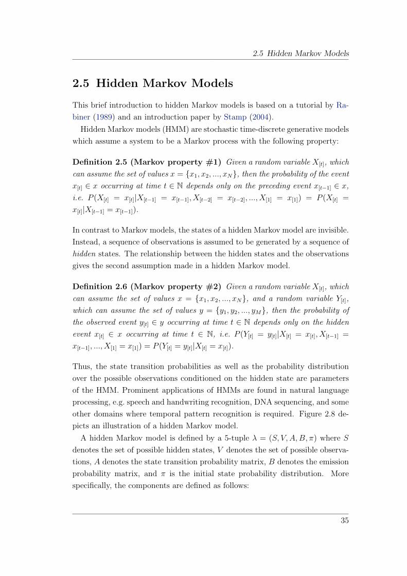
2.5 Hidden Markov Models
2.5 Hidden Markov Models
This brief introduction to hidden Markov models is based on a tutorial by Ra-
biner (1989) and an introduction paper by Stamp (2004).
Hidden Markov models (HMM) are stochastic time-discrete generative models
which assume a system to be a Markov process with the following property:
Definition 2.5 (Markov property #1) Given a random variable X[t], which
can assume the set of values x = x1, x2, ..., xN, then the probability of the event
x[t] ∈ x occurring at time t ∈ N depends only on the preceding event x[t−1] ∈ x,
i.e. P (X[t] = x[t]|X[t−1] = x[t−1], X[t−2] = x[t−2], ..., X[1] = x[1]) = P (X[t] =
x[t]|X[t−1] = x[t−1]).
In contrast to Markov models, the states of a hidden Markov model are invisible.
Instead, a sequence of observations is assumed to be generated by a sequence of
hidden states. The relationship between the hidden states and the observations
gives the second assumption made in a hidden Markov model.
Definition 2.6 (Markov property #2) Given a random variable X[t], which
can assume the set of values x = x1, x2, ..., xN, and a random variable Y[t],
which can assume the set of values y = y1, y2, ..., yM, then the probability of
the observed event y[t] ∈ y occurring at time t ∈ N depends only on the hidden
event x[t] ∈ x occurring at time t ∈ N, i.e. P (Y[t] = y[t]|X[t] = x[t], X[t−1] =
x[t−1], ..., X[1] = x[1]) = P (Y[t] = y[t]|X[t] = x[t]).
Thus, the state transition probabilities as well as the probability distribution
over the possible observations conditioned on the hidden state are parameters
of the HMM. Prominent applications of HMMs are found in natural language
processing, e.g. speech and handwriting recognition, DNA sequencing, and some
other domains where temporal pattern recognition is required. Figure 2.8 de-
picts an illustration of a hidden Markov model.
A hidden Markov model is defined by a 5-tuple λ = (S, V,A,B, π) where S
denotes the set of possible hidden states, V denotes the set of possible observa-
tions, A denotes the state transition probability matrix, B denotes the emission
probability matrix, and π is the initial state probability distribution. More
specifically, the components are defined as follows:
35

2 Theoretical Background
Markov process s[t−1] s[t] s[t+1]A A
Observations v[t−1] v[t] v[t+1]
B B B
Figure 2.8: Hidden Markov model
• S = s1, s2, ..., sN is the set of unobserved states which are the possible
values of the random variable X[t] at time t ∈ N.
• V = v1, v2, ..., vM is the set of possible observations being the emissions
of the random variable Y[t] at time t ∈ N.
• A ∈ [0, 1]N×N is the state transition probability matrix modeling P (X[t+1] =
sj|X[t] = si) = Aij where∑Nj=1Aij = 1 ∀j ∈ 1, 2, ..., N.
• B ∈ [0, 1]n×m is the emission matrix where bi(vj) = P (Y[t] = vj|X[t] = si)
is the probability of making the observation vj given the unobserved state
si.
• π ∈ [0, 1]N is the initial probability distribution over the states S, i.e.
P (X[1] = si) = πi where∑Ni=1 πi = 1.
Thus, the parameters of the hidden Markov model are summarized as θ =
A,B, π. A common and natural assumption is to constrain the state tran-
sition probabilities A and the emission matrix B to be time-invariant, i.e. the
probabilities do not change over time.
A hidden Markov model may be used in several inference scenarios.
Decoding/Filtering. Given the parameters θ of the model, the probability dis-
tribution π over the initial states, and a sequence of observations (Y[1], Y[2], ..., Y[T ]),
the task is to determine the probability distribution over the hidden states
X[T ] after T time steps, i.e. P (X[T ]|Y[1], X[2], ..., Y[T ]). The hidden Markov
model assumes that the underlying process moves through a sequence of
states which emit the corresponding observations (Y[1], Y[2], ..., Y[T ]).
36

2.5 Hidden Markov Models
Smoothing. Given the parameters θ of the model, the probability distribution
π over the initial states, and a sequence of observations (Y[1], Y[2], ..., Y[T ]),
the task is to determine the probability distribution over the hidden states
X[T−∆t] after T − ∆t time steps with ∆t ∈ N and 1 < ∆t < T , i.e.
P (X[T−∆t]|Y[1], X[2], ..., Y[T ]). This task is similar to the decoding/filtering
task, but instead of predicting the hidden state distribution at the end of
the observed sequence, it shall be predicted somewhere in the middle of
the sequence.
Prediction. Given the parameters θ of the model, the probability distribution
π over the initial states, a sequence of observations (Y[1], Y[2], ..., Y[T ]), and
a non-negative integer ∆t, the task is to determine the probability distri-
bution over the hidden states X[T+∆t] after T + ∆t ∈ N time steps, i.e.
P (X[T+∆t]|Y[1], X[2], ..., Y[T ]). This task is similar to the decoding/filtering
task, but instead of predicting the hidden state distribution at the end of
the observed sequence, it shall be predicted after an additional ∆t time
steps without the availability of further observations from the ∆t addi-
tional time steps.
Learning. Given a sequence of observations Y = (Y[1], Y[2], ..., Y[T ]), the task is
to determine the parameters θ∗ which maximize the probability of the
observed sequence given a hidden state sequence X = (X[1], X[2], ..., X[T ]),
i.e.
θ∗ = arg maxθ
P (Y ) (2.25a)
= arg maxθ
∑
X
P (Y,X) (2.25b)
= arg maxθ
∑
X
P (Y |X)P (X) (2.25c)
= arg maxθ
∑
X
T∏
t=1
P (X[t]|X[t−1], X[t−2], ..., X[1])P (Y[t]|X[t]) (2.25d)
= arg maxθ
∑
X
T∏
t=1
P (X[t]|X[t−1])P (Y[t]|X[t]). (2.25e)
Given the learned parameters θ∗, it is possible to determine the probability
of a new observed sequence under the model.
37
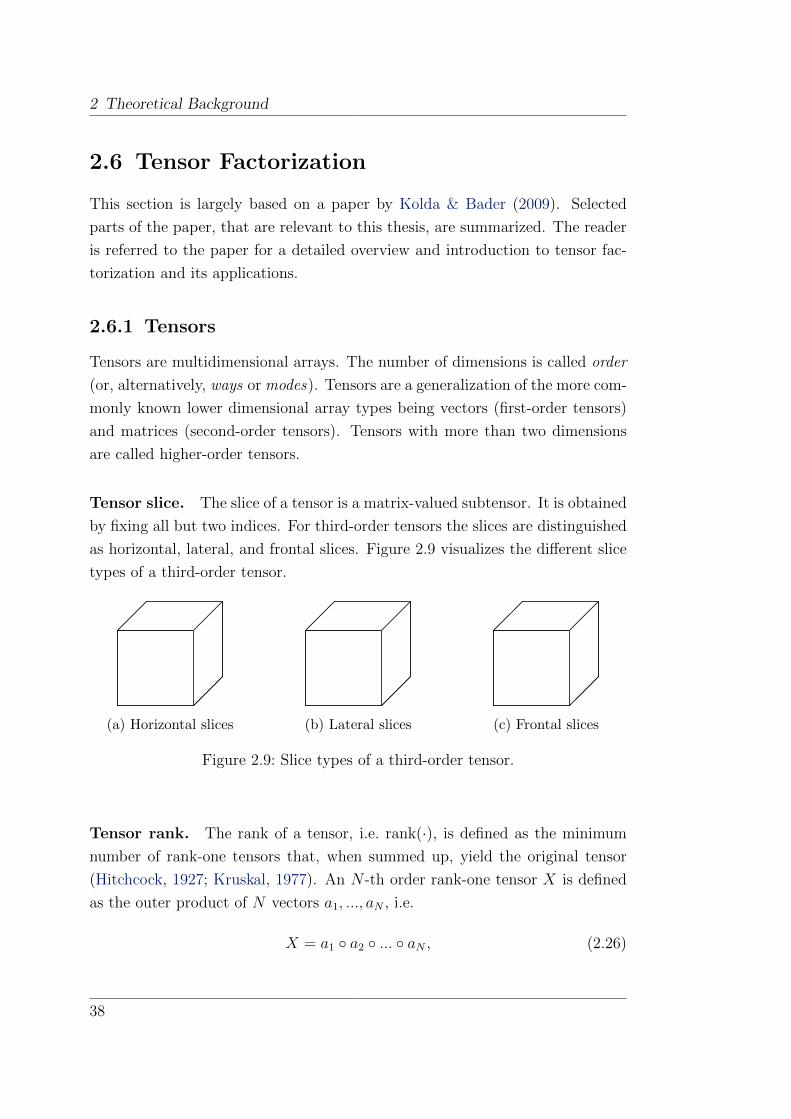
2 Theoretical Background
2.6 Tensor Factorization
This section is largely based on a paper by Kolda & Bader (2009). Selected
parts of the paper, that are relevant to this thesis, are summarized. The reader
is referred to the paper for a detailed overview and introduction to tensor fac-
torization and its applications.
2.6.1 Tensors
Tensors are multidimensional arrays. The number of dimensions is called order
(or, alternatively, ways or modes). Tensors are a generalization of the more com-
monly known lower dimensional array types being vectors (first-order tensors)
and matrices (second-order tensors). Tensors with more than two dimensions
are called higher-order tensors.
Tensor slice. The slice of a tensor is a matrix-valued subtensor. It is obtained
by fixing all but two indices. For third-order tensors the slices are distinguished
as horizontal, lateral, and frontal slices. Figure 2.9 visualizes the different slice
types of a third-order tensor.
(a) Horizontal slices (b) Lateral slices (c) Frontal slices
Figure 2.9: Slice types of a third-order tensor.
Tensor rank. The rank of a tensor, i.e. rank(·), is defined as the minimum
number of rank-one tensors that, when summed up, yield the original tensor
(Hitchcock, 1927; Kruskal, 1977). An N -th order rank-one tensor X is defined
as the outer product of N vectors a1, ..., aN , i.e.
X = a1 a2 ... aN , (2.26)
38
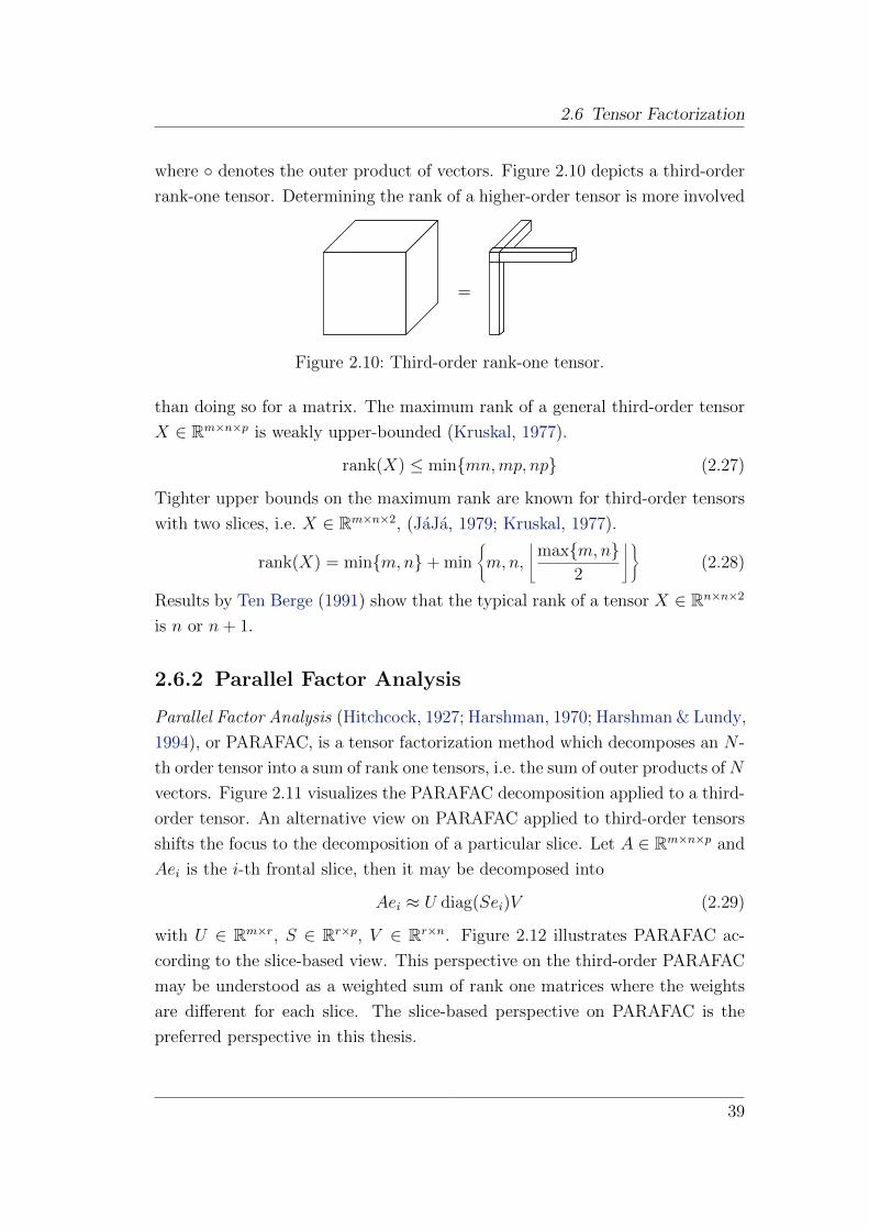
2.6 Tensor Factorization
where denotes the outer product of vectors. Figure 2.10 depicts a third-order
rank-one tensor. Determining the rank of a higher-order tensor is more involved
=
Figure 2.10: Third-order rank-one tensor.
than doing so for a matrix. The maximum rank of a general third-order tensor
X ∈ Rm×n×p is weakly upper-bounded (Kruskal, 1977).
rank(X) ≤ minmn,mp, np (2.27)
Tighter upper bounds on the maximum rank are known for third-order tensors
with two slices, i.e. X ∈ Rm×n×2, (JaJa, 1979; Kruskal, 1977).
rank(X) = minm,n+ min
®m,n,
úmaxm,n
2
ü´(2.28)
Results by Ten Berge (1991) show that the typical rank of a tensor X ∈ Rn×n×2
is n or n+ 1.
2.6.2 Parallel Factor Analysis
Parallel Factor Analysis (Hitchcock, 1927; Harshman, 1970; Harshman & Lundy,
1994), or PARAFAC, is a tensor factorization method which decomposes an N -
th order tensor into a sum of rank one tensors, i.e. the sum of outer products ofN
vectors. Figure 2.11 visualizes the PARAFAC decomposition applied to a third-
order tensor. An alternative view on PARAFAC applied to third-order tensors
shifts the focus to the decomposition of a particular slice. Let A ∈ Rm×n×p and
Aei is the i-th frontal slice, then it may be decomposed into
Aei ≈ U diag(Sei)V (2.29)
with U ∈ Rm×r, S ∈ Rr×p, V ∈ Rr×n. Figure 2.12 illustrates PARAFAC ac-
cording to the slice-based view. This perspective on the third-order PARAFAC
may be understood as a weighted sum of rank one matrices where the weights
are different for each slice. The slice-based perspective on PARAFAC is the
preferred perspective in this thesis.
39
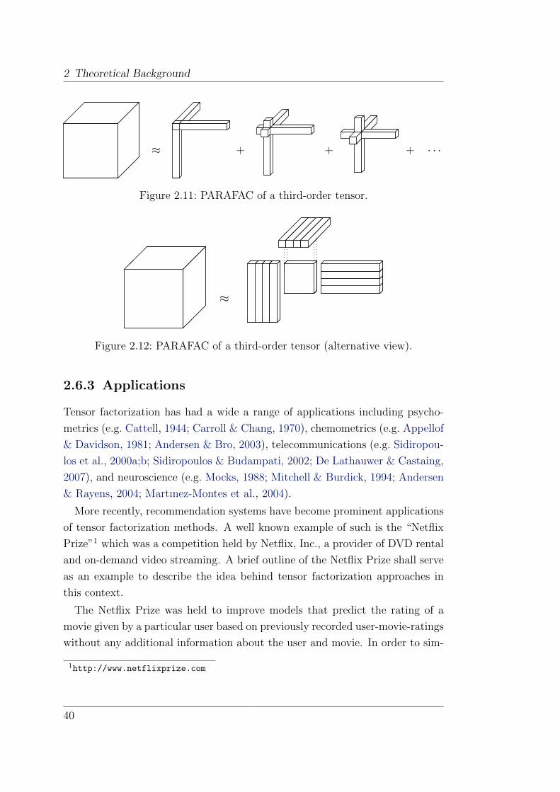
2 Theoretical Background
≈ + + + · · ·
Figure 2.11: PARAFAC of a third-order tensor.
≈
Figure 2.12: PARAFAC of a third-order tensor (alternative view).
2.6.3 Applications
Tensor factorization has had a wide a range of applications including psycho-
metrics (e.g. Cattell, 1944; Carroll & Chang, 1970), chemometrics (e.g. Appellof
& Davidson, 1981; Andersen & Bro, 2003), telecommunications (e.g. Sidiropou-
los et al., 2000a;b; Sidiropoulos & Budampati, 2002; De Lathauwer & Castaing,
2007), and neuroscience (e.g. Mocks, 1988; Mitchell & Burdick, 1994; Andersen
& Rayens, 2004; Martınez-Montes et al., 2004).
More recently, recommendation systems have become prominent applications
of tensor factorization methods. A well known example of such is the “Netflix
Prize”1 which was a competition held by Netflix, Inc., a provider of DVD rental
and on-demand video streaming. A brief outline of the Netflix Prize shall serve
as an example to describe the idea behind tensor factorization approaches in
this context.
The Netflix Prize was held to improve models that predict the rating of a
movie given by a particular user based on previously recorded user-movie-ratings
without any additional information about the user and movie. In order to sim-
1http://www.netflixprize.com
40

2.6 Tensor Factorization
plify the illustration of tensor factorization, the date of the rating is ignored
in this example. The set of triples (user,movie, rating), where the users and
movies are encoded as nonnegative integers and the ratings are values in the set
1, 2, 3, 4, 5, can be represented by a sparse matrix X ∈ 0, 1, ..., 5#users×#movies
where a zero represents a missing rating of a particular movie given by a partic-
ular user. The matrix is sparse because most users have only rated a few movies.
Figure 2.13 illustrates the user-movie-ratings matrix. Factorization of this rat-
3 4 1 0 0 1 · · · 5
0 0 0 0 1 1 · · · 0
0 0 0 5 4 0 · · · 0
0 3 0 3 3 0 · · · 3
0 0 0 0 0 0 · · · 4
......
......
......
...
1 0 2 0 0 0 · · · 0
∼ 17 700 movies
∼480000users
Figure 2.13: Example of the Netflix user-movie-ratings matrix.
ing matrix into low-rank components of the users and movies, i.e. PARAFAC in
two dimensions, was a basic approach in the competition. Figure 2.14 depicts
the low-rank factorization of the rating matrix. When fitted to the data matrix,
latent representations of the users and movies are obtained whose pairwise inner
products approximate the corresponding ratings in the rating matrix. The num-
ber of latent factors affects the rank of the approximated rating matrix. After
learning the components, it turns out that they can be interpreted as properties
of the users and movies, e.g.
• the movie may have a particular genre such as “action” and a user with
this genre preference will be more likely to give a high rating;
• the movie may be serious in some sense and a user with a preference for
41
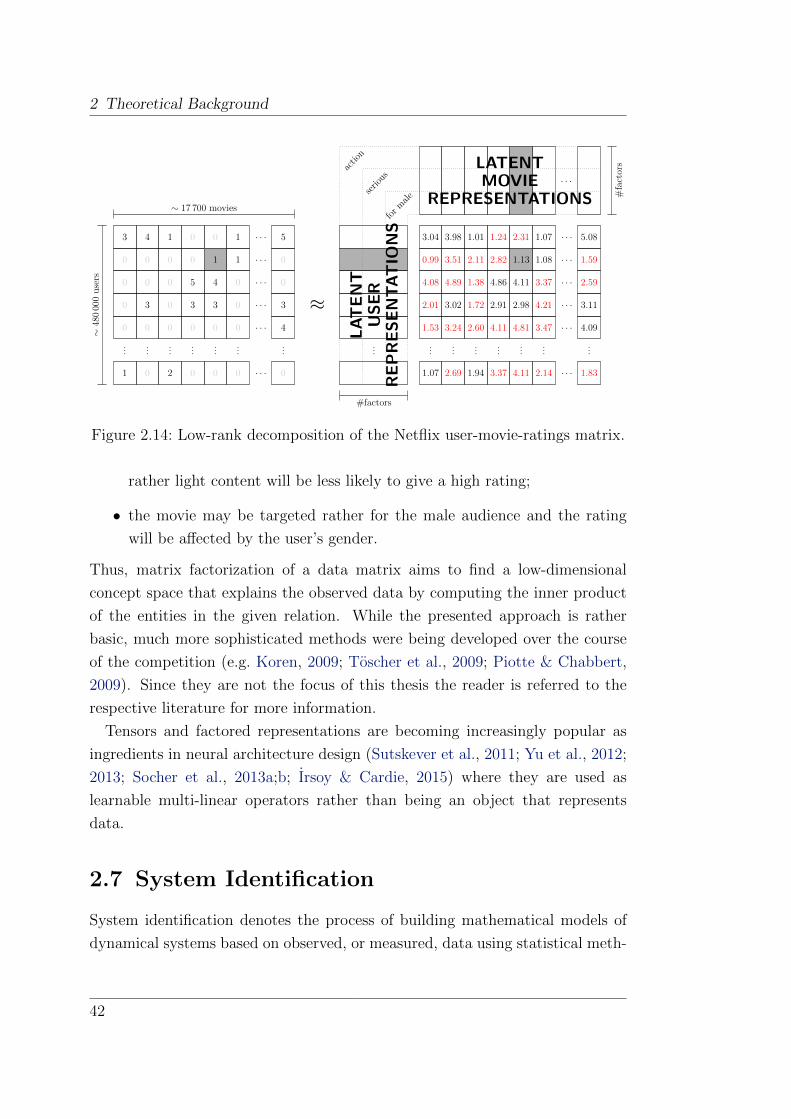
2 Theoretical Background
3 4 1 0 0 1 · · · 5
0 0 0 0 1 1 · · · 0
0 0 0 5 4 0 · · · 0
0 3 0 3 3 0 · · · 3
0 0 0 0 0 0 · · · 4
......
......
......
...
1 0 2 0 0 0 · · · 0
∼ 17 700 movies
∼480000users
≈...
· · ·
3.04 3.98 1.01 1.24 2.31 1.07 · · · 5.08
0.99 3.51 2.11 2.82 1.13 1.08 · · · 1.59
4.08 4.89 1.38 4.86 4.11 3.37 · · · 2.59
2.01 3.02 1.72 2.91 2.98 4.21 · · · 3.11
1.53 3.24 2.60 4.11 4.81 3.47 · · · 4.09
......
......
......
...
1.07 2.69 1.94 3.37 4.11 2.14 · · · 1.83
#factors
#factorsac
tion
serious
for m
ale
LATENT
USER
REPRESENTATIO
NS
LATENTMOVIE
REPRESENTATIONS
Figure 2.14: Low-rank decomposition of the Netflix user-movie-ratings matrix.
rather light content will be less likely to give a high rating;
• the movie may be targeted rather for the male audience and the rating
will be affected by the user’s gender.
Thus, matrix factorization of a data matrix aims to find a low-dimensional
concept space that explains the observed data by computing the inner product
of the entities in the given relation. While the presented approach is rather
basic, much more sophisticated methods were being developed over the course
of the competition (e.g. Koren, 2009; Toscher et al., 2009; Piotte & Chabbert,
2009). Since they are not the focus of this thesis the reader is referred to the
respective literature for more information.
Tensors and factored representations are becoming increasingly popular as
ingredients in neural architecture design (Sutskever et al., 2011; Yu et al., 2012;
2013; Socher et al., 2013a;b; Irsoy & Cardie, 2015) where they are used as
learnable multi-linear operators rather than being an object that represents
data.
2.7 System Identification
System identification denotes the process of building mathematical models of
dynamical systems based on observed, or measured, data using statistical meth-
42
2.8 Artificial Benchmarks
ods. Such models are typically distinguished as white, grey, and black box mod-
els. White box models are usually based on the fundamentals of physics, e.g.
Newton’s laws of motion, but they often become too complex or even impossible
to derive in real-world applications. Grey box models are hybrids that rely on
both a basic understanding of the system as well as on experimental data to
estimate remaining unknown parameters. Grey box models are also known as
semi-physical models (Forssell & Lindskog, 1997). Black box models rely en-
tirely on observed measurements without utilizing any prior model. They are
particularly common and useful when the system is poorly understood and/or
very complex to describe using analytical methods. In this thesis black box
models are investigated.
2.8 Artificial Benchmarks
This section introduces two artificial benchmarks which are well known in the
reinforcement learning community. Their dynamics are described analytically
and, thus, enable sampling data from varying configurations. Being able to
easily generate data from similar dynamical systems is an important requirement
in this thesis.
2.8.1 Cart-Pole
The cart-pole simulation (Michie & Chambers, 1968a;b; Barto et al., 1983; Sut-
ton & Barto, 1998; Florian, 2007) consists of a cart, which moves on a one-
dimensional track, and a pole hinged to the cart. Two control problems are
commonly addressed in the context of this dynamical system: the pole swing-
up task and the balancing task. In the swing-up task, the pole initially hangs
downward and shall be swung up such that it is finally balanced in an upright
position. The swing-up is achieved by applying an appropriate action sequence,
i.e. a force applied to the cart, using as few steps as possible. The balancing
task is a subtask of the swing-up task in which the pole starts in an upright
position and shall remain balanced. Figure 2.15 depicts an illustration of the
cart-pole environment. The state description consists of the tuple (x, x, α, α)
being the position x ∈ R and velocity x ∈ R of the cart as well as the angle
α ∈]−180°, 180°] and angular velocity α ∈ R of the pole. Contrary to settings
43
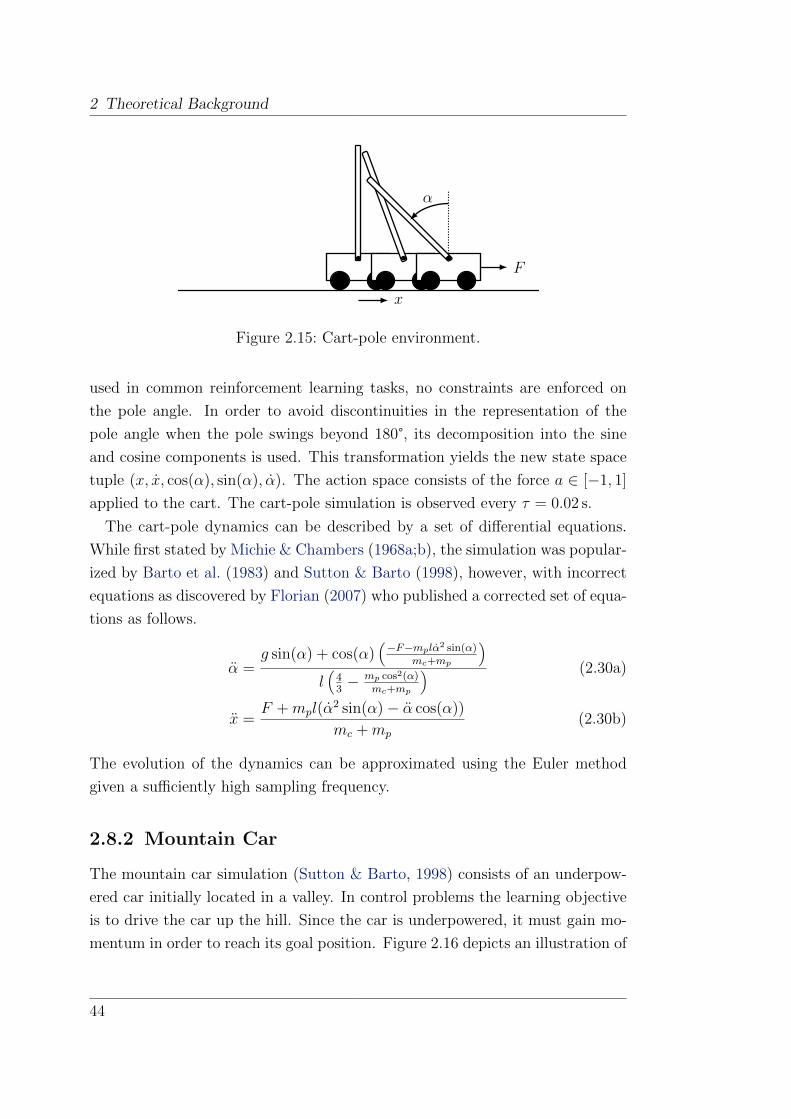
2 Theoretical Background
−2.4 2.4x
F
α
Figure 2.15: Cart-pole environment.
used in common reinforcement learning tasks, no constraints are enforced on
the pole angle. In order to avoid discontinuities in the representation of the
pole angle when the pole swings beyond 180°, its decomposition into the sine
and cosine components is used. This transformation yields the new state space
tuple (x, x, cos(α), sin(α), α). The action space consists of the force a ∈ [−1, 1]
applied to the cart. The cart-pole simulation is observed every τ = 0.02 s.
The cart-pole dynamics can be described by a set of differential equations.
While first stated by Michie & Chambers (1968a;b), the simulation was popular-
ized by Barto et al. (1983) and Sutton & Barto (1998), however, with incorrect
equations as discovered by Florian (2007) who published a corrected set of equa-
tions as follows.
α =g sin(α) + cos(α)
(−F−mplα2 sin(α)mc+mp
)
l(
43− mp cos2(α)
mc+mp
) (2.30a)
x =F +mpl(α
2 sin(α)− α cos(α))
mc +mp
(2.30b)
The evolution of the dynamics can be approximated using the Euler method
given a sufficiently high sampling frequency.
2.8.2 Mountain Car
The mountain car simulation (Sutton & Barto, 1998) consists of an underpow-
ered car initially located in a valley. In control problems the learning objective
is to drive the car up the hill. Since the car is underpowered, it must gain mo-
mentum in order to reach its goal position. Figure 2.16 depicts an illustration of
44

2.9 Implementation
f(x) = 13sin(3x)x
F
−0.5−1.2 0.6
Figure 2.16: Mountain car environment.
the mountain car environment. The mountain shape follows the trigonometric
function f(x) = 13
sin(3x). The state description consists of the tuple (x, x),
x ∈ [−1.2, 0.6] and x ∈ [−0.07, 0.07], being the position and velocity of the car.
The action space consists of the acceleration a ∈ −1, 0, 1 of the car which
is altered to be continuous-valued in this thesis, i.e. a ∈ [−1, 1], to make the
simulation more realistic.
The mountain car dynamics can be described by the following update equa-
tions with typical values of the acceleration factor γ = 0.001 and the gravity
g = −0.0025.
x[t+1] = x[t] + γa+ g cos(3x) (2.31a)
x[t+1] = x[t] + x[t+1] (2.31b)
2.9 Implementation
All model implementations are based on Theano (Bergstra et al., 2010; Bastien
et al., 2012). “Theano is a Python library that allows you to define, optimize,
and evaluate mathematical expressions involving multi-dimensional arrays effi-
ciently.”2 Theano allows to express a model, the objective to be optimized as
well as the optimization algorithm through a symbolic graph of mathematical
2http://deeplearning.net/software/theano
45

2 Theoretical Background
symbolic types, e.g. scalar, vector, matrix, etc., and operations, e.g. matrix-
vector,matrix multiplication, elementwise functions, slicing/indexing. Defin-
ing a computational graph follows NumPy’s interface very closely making it
convenient to use and easy to adopt. Defining computations symbolically im-
plies several advantages over “direct” implementations. First and foremost, a
symbolically defined optimization objective allows for automatic differentiation
which is a core ingredient in many machine learning algorithms in order to fit
the model parameters to data. Automatic differentiation is not only conve-
nient it also accelerates the prototyping of new models as well as reduces errors
in taking and implementing derivatives manually. Second, the availability of
the computational graph in symbolical form allows for graph optimization that
may replace expression patterns by equivalent but computationally faster and/or
numerically more stable expressions. The graph optimization framework also
enables substituting generic operations, that would eventually be executed on
the CPU, by other implementations, that may be executed on a different device
such as a GPU. Third, once a graph is optimized it gets compiled on-the-fly
by automatically generating C/C++/CUDA/OpenCL code and executing the
corresponding native compiler. A compiled function is transparently accessible
from within Python.
Listing 1 depicts code of a logistic regression model that illustrates the usage
of Theano.
46
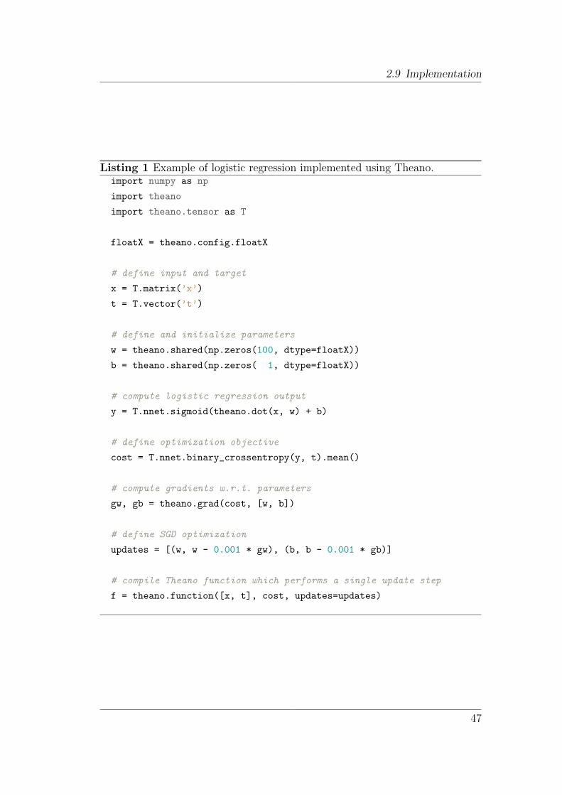
2.9 Implementation
Listing 1 Example of logistic regression implemented using Theano.import numpy as np
import theano
import theano.tensor as T
floatX = theano.config.floatX
# define input and target
x = T.matrix(’x’)
t = T.vector(’t’)
# define and initialize parameters
w = theano.shared(np.zeros(100, dtype=floatX))
b = theano.shared(np.zeros( 1, dtype=floatX))
# compute logistic regression output
y = T.nnet.sigmoid(theano.dot(x, w) + b)
# define optimization objective
cost = T.nnet.binary_crossentropy(y, t).mean()
# compute gradients w.r.t. parameters
gw, gb = theano.grad(cost, [w, b])
# define SGD optimization
updates = [(w, w - 0.001 * gw), (b, b - 0.001 * gb)]
# compile Theano function which performs a single update step
f = theano.function([x, t], cost, updates=updates)
47

2 Theoretical Background
48
CHAPTER 3
Multi-Task and Transfer Learning with
Recurrent Neural Networks
This chapter presents recurrent neural network architectures that are capable
of transferring knowledge among related sequence learning tasks by means of
parameter sharing. First the meaning, utility, and relatedness of multi-task and
transfer learning is discussed (Section 3.1). Second, terminological differences
and similarities between the learning paradigms multi-task and transfer learn-
ing are scrutinized in order to clearly distinguish the implications of both terms
(Section 3.2). Third, three recurrent neural networks architectures suitable for
multi-task and transfer learning on sequential data are introduced (Section 3.3).
They form the conceptual bases of the models used in the subsequent chapters.
Two simple approaches to learning joint models of multiple tasks are introduced
and discussed. Thereafter, the Factored Tensor Recurrent Neural Network ar-
chitecture is presented which is one of the main contributions of this thesis.
Its natural way of incorporating task-specific as well as cross-task parameters
is elaborated on by drawing the connection between recurrent neural language
modeling and multi-task and transfer learning with factored tensor parameters
on sequential data.
The subsequent sections are based on the following list of publications as part
of the doctoral research:
• Spieckermann, S., Dull, S., Udluft, S., Hentschel, A., and Runkler, T.
Exploiting similarity in system identification tasks with recurrent neural
networks. In Proceedings of the 22nd European Symposium on Artifi-
cial Neural Networks, Computational Intelligence and Machine Learning
(ESANN), 2014a.
49

3 Multi-Task and Transfer Learning with Recurrent Neural Networks
• Spieckermann, S., Dull, S., Udluft, S., Hentschel, A., and Runkler, T.
Exploiting similarity in system identification tasks with recurrent neural
networks. Neurocomputing, (Special Issue ESANN 2014), 2015. Extended
version. Invited paper.
• Spieckermann, S., Dull, S., Udluft, S., and Runkler, T. Multi-system iden-
tification for efficient knowledge transfer with factored tensor recurrent
neural networks. In Proceedings of the European Conference on Machine
Learning (ECML), Workshop on Generalization and Reuse of Machine
Learning Models over Multiple Contexts, 2014b.
3.1 Multi-Task Learning
Multi-task learning is a learning paradigm in machine learning that aims to
reduce the model error of a target task by utilizing related auxiliary learning
tasks. Thus, the model exploits commonalities among the provided tasks where
the auxiliary tasks serve as an inductive bias. “Inductive bias is anything that
causes an inductive learner to prefer some hypotheses over other hypotheses.
Bias-free learning is impossible; much of the power of an inductive learner follows
directly from the power of its inductive bias (Mitchell, 1980). [...] One does not
usually think of training signals as a bias; but when the training signals are for
tasks other than the main task, it is easy to see that, from the point of view
of the main task, the other tasks may serve as a bias.” (Caruana, 1997) This
approach often leads to improved generalization due to inductive transfer.
Multi-task learning can happen in multiple ways. Let (x, y) denote a training
example consisting of an input vector x and a target y in a supervised learning
problem. Instead of simply learning the mapping from x to y, it may be possible
to come up with additional targets (y′, y′′, ...) whose error signals help guide
the learning process to discover more robust and generally useful patterns in
the inputs across a variety of related tasks. The resulting model may share
the parameters of its feature extraction component, e.g. the input-to-hidden
weights of a feed-forward neural network, and predict the targets based on the
cross-task hidden representation. Another common approach is to couple task-
specific parameters by means of regularization to enforce information sharing.
Alternatively, a training example (i, x, y) may originate from a specific task
50

3.2 Multi-Task vs. Transfer Learning
indexed i while all tasks share a common target y. The tasks then differ in
terms of their mapping from x to y. The latter scenario will be investigated in
this thesis.
3.2 Multi-Task vs. Transfer Learning
Multi-task and transfer learning are two related learning paradigms with similar
goals but different angles of approach. The common goal of both paradigms is
to reduce the model error of the target model by utilizing one or multiple related
auxiliary task(s).
Caruana (1997) distinguishes between parallel and sequential transfer where
parallel transfer is performed through multi-task learning and sequential transfer
translates to transfer learning. Multi-task learning means to learn a joint model
of all tasks, i.e. the target task and all auxiliary tasks, simultaneously. In
contrast, transfer learning implies a sequence in which the models are learned.
Typically, the target task is learned subsequent to the auxiliary tasks. Thus,
the target task learning process cannot interact with the auxiliary tasks.
Another perspective was formulated by Pan & Yang (2010). They distinguish
multi-task and transfer learning as follows: “[...] transfer learning aims to ex-
tract the knowledge from one or more source tasks and applies the knowledge to
a target task. In contrast to multitask learning, rather than learning all of the
source and target tasks simultaneously, transfer learning cares most about the
target task. The roles of the source and target tasks are no longer symmetric
in transfer learning.”
3.3 Multi-Task Recurrent Neural Networks
This section identifies a number of neural network based models that enable
multi-task learning of sequential data. While there are many ways to implement
multi-task learning, this chapter focuses on parameter sharing approaches where
data-efficiency is obtained by using many cross-task and few task-specific pa-
rameters. An RNN as introduced in Section 2.3.3 may allocate task-specific pa-
rameters in the input-to-hidden, hidden-to-hidden, and hidden-to-output trans-
formations. Making one of those components task-specific has implications on
51
3 Multi-Task and Transfer Learning with Recurrent Neural Networks
the nature of the tasks, in what aspects they are similar and dissimilar, and
how this knowledge can be incorporated into the joint model. For instance, in
natural language processing a sequence of words may be subject to multiple si-
multaneous classification tasks such as sentiment classification of a sentence and
named entity recognition of each word. A typical approach would be to have a
cross-task recurrent feature extraction and task-specific classification layers fol-
lowing the assumption that features of the two tasks may be mutually beneficial
because they reveal more information about the overall problem structure. Al-
ternatively, multiple tasks may share the same learning problem, but the input
data may originate from different domains. For instance, product reviews in an
online shop may be available from different product categories and the task is
to infer their sentiment. In this case, the feature extraction may be task-specific
while the classification submodel is the same for both tasks.
The following subsections present variants of RNN models that are general
in concept but selected with system identification tasks in mind. It is assumed
that the different tasks have identical input and output spaces.
3.3.1 Naıve RNN
The most naıve approach of multi-task learning is to learn a joint model for
all tasks. Figure 2.6 depicts a graphical representation of the model. The data
of all tasks are concatenated prior to learning. Thus, the joint model needs to
generalize over all tasks. Generalization is possible if the factors that distinguish
the tasks can be quantified and are observable. Making them available to the
model allows for task discrimination. Otherwise, the model can only learn the
average task at best and should be inferior to simple ways of incorporating task-
discriminating information. This model serves as a baseline to ensure that tasks
are in fact non-identical or to indicate that task-discriminating information is
not available.
3.3.2 RNN+ID
In absence of task-discriminating factors, a simple way to distinguish the tasks
is to tag each task with a positive integer task identifier i ∈ I, i.e. the training
examples of each task are tagged and concatenated to form a multi-task data
52

3.3 Multi-Task Recurrent Neural Networks
set. This tag may be provided to the model at each sequential step as an extra
input encoded as the i-th Euclidean standard basis vector ei with dim(ei) = |I|also known as “one-hot” encoding. The equations of the RNN+ID architecture
are obtained by substituting (2.14b) with (3.1).
h[t] = φh(Whxx[t] +Whhh[t−1] +Whiei + bh) (3.1)
Figure 3.1 depicts a graphical representation of the RNN+ID architecture. In
x[t−1] x[t] x[t+1]
1 1 1
h[t−1] h[t] h[t+1]
Whx Whx Whxei ei ei
Whh Whh
y[t−1] y[t] y[t+1]
Wyh Wyh Wyh
b h b h b h
b y b y b y
Figure 3.1: RNN+ID architecture for multi-task learning on sequential inputs.
fact, computing Whiei means selecting the i-th column of Whi so the system
identifier introduces a separate bias for each system. The cross-system bias
bh and the specific biases accessed through Whiei can be absorbed into a new
system-specific bias ›Whiei = bh +Whiei. Thus, (3.1) can be rewritten as
h[t] = φh(Whxx[t] +Whhh[t−1] +›Whiei). (3.2)
3.3.3 Factored Tensor Recurrent Neural Network
(FTRNN)
The previous subsection showed that providing the network with a “one-hot”
encoded system identifier ei is in fact equivalent to learning a different hidden
layer bias ›Whiei for each system. The bias of a particular neuron determines its
53

3 Multi-Task and Transfer Learning with Recurrent Neural Networks
activity threshold. Making the bias task-specific thus allows to learn a different
threshold for each task. However, the main transformation from one layer is due
to a parameter matrix Wvu ∈ Rnv×nu , so it is a natural choice to use a different
parameter matrix Wvu for each task. Multiple such matrices can be viewed as
frontal slices of a third-order tensor Wvui ∈ Rnv×nu×|I|.
The primary source of the idea that yields the model of this subsection is
a paper on character-level language modeling using recurrent neural networks
(Sutskever et al., 2011). Language modeling is commonly defined as the task
of assigning the probability of occurrences to a given sequence of words. That
is, given a word vocabulary V and a sequence of words (w[1], ..., w[k]), w[i] ∈V , the language model yields P (w[1], ..., w[k]). By using the chain rule this
joint probability can be decomposed into factors of conditional probabilities as
follows.
P (w[1], ..., w[k]) = P (w[k]|w[1], ..., w[k−1])P (w[k−1]|w[1], ..., w[k−2]) · · · (3.3a)
= P (w[1])k∏
i=2
P (w[i]|w[1], ..., w[i−1]) (3.3b)
Recurrent neural networks are a natural and effective choice to estimate the
conditional probabilities (Mikolov et al., 2010). However, Sutskever et al. ar-
gue that a modified architecture with so-called “multiplicative” connections is
superior to the standard architecture in the character-level language modeling
task. Multiplicative interactions are derived as follows. In order to improve the
expressiveness of the model the parameter matrix Whh is conditioned on the
current input character, thus, yielding a different state transition per charac-
ter. Naıvely, the parameters would be stored in a third-order tensor where each
slice represents the transition matrix of a particular character in the vocabulary.
Although the vocabulary of characters is much smaller than the prohibitively
large vocabulary of words the size of the three-way tensor is impractical never-
theless. Sutskever et al. propose to learn a factored representation as used by
Taylor & Hinton (2009), who model multiple motion styles from images using
Restricted Boltzmann Machines. While not explicitly stated in any of the papers
the proposed factorization is known as Parallel Factor Analysis (PARAFAC, see
Section 2.6.2 for details) for three-way tensors where the vectors of the third
mode can be viewed as latent representations, or factors, of each character that
adjust the state transition matrix.
54
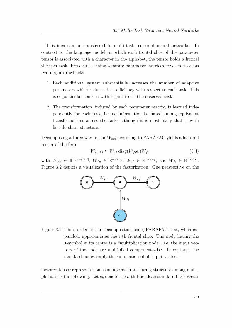
3.3 Multi-Task Recurrent Neural Networks
This idea can be transferred to multi-task recurrent neural networks. In
contrast to the language model, in which each frontal slice of the parameter
tensor is associated with a character in the alphabet, the tensor holds a frontal
slice per task. However, learning separate parameter matrices for each task has
two major drawbacks.
1. Each additional system substantially increases the number of adaptive
parameters which reduces data efficiency with respect to each task. This
is of particular concern with regard to a little observed task.
2. The transformation, induced by each parameter matrix, is learned inde-
pendently for each task, i.e. no information is shared among equivalent
transformations across the tasks although it is most likely that they in
fact do share structure.
Decomposing a three-way tensor Wvui according to PARAFAC yields a factored
tensor of the form
Wvuiei ≈ Wvf diag(Wfiei)Wfu (3.4)
with Wvui ∈ Rnv×nu×|I|, Wfu ∈ Rnf×nu , Wvf ∈ Rnv×nf , and Wfi ∈ Rnf×|I|.
Figure 3.2 depicts a visualization of the factorization. One perspective on the
ei
u v•
Wfi
Wfu Wvf
Figure 3.2: Third-order tensor decomposition using PARAFAC that, when ex-
panded, approximates the i-th frontal slice. The node having the
•-symbol in its center is a “multiplication node”, i.e. the input vec-
tors of the node are multiplied component-wise. In contrast, the
standard nodes imply the summation of all input vectors.
factored tensor representation as an approach to sharing structure among multi-
ple tasks is the following. Let ek denote the k-th Euclidean standard basis vector
55

3 Multi-Task and Transfer Learning with Recurrent Neural Networks
with an appropriate dimensionality, eTkWfu is the k-th row of Wfu, Wvfek is the
k-th column of Wvf and eTkWfiei is the k-th element of the diagonal matrix
diag(Wfiei). Expanding the i-th slice of the factored tensor, i.e. the expanded
parameter matrix for system i ∈ I, can be written as the weighted sum of
rank-one matrices (Wvfek)ÄeTkWfu
ä, i.e.
Wvuiei ≈nf∑
k=1
(Wvfek)ÄeTkWfiei
ä ÄeTkWfu
ä. (3.5)
The equality of (3.4) and (3.5) can be shown as follows. Let v ∈ Rn be an n-
dimensional column vector whose k-th element denotes vk = eTk v. The diag(v)
operator maps the vector v to a diagonal matrix in Rn×n and is defined as
follows.
diag(v) :=∑
k
ekeTk vk (3.6)
In the following, let [W ]ab denote the element of the matrix W at row a and
column b. Using (3.6), the diagonal matrix diag(Wfiei) can be written as
diag(Wfiei) = diag
ÑÑ∑
a,b
[Wfi]abeaeTb
éei
é(3.7a)
= diag
Ñ∑
a,b
[Wfi]abea(eTb ei)
é(3.7b)
= diag
Ñ∑
a,b
[Wfi]abeaδbi
é(3.7c)
= diag
Ç∑a
[Wfi]aiea
å(3.7d)
=∑
k
ekeTk
ÇeTk∑
a
[Wfi]aiea
å(3.7e)
=∑
k,a
ekeTk e
Tk ea[Wfi]ai (3.7f)
=∑
k,a
ekeTk δka[Wfi]ai (3.7g)
=∑
k
ekeTk [Wfi]ki (3.7h)
=∑
k
ek[Wfi]kieTk . (3.7i)
56

3.3 Multi-Task Recurrent Neural Networks
Substituting this result in (3.5) yields
Wvuiei ≈ Wvf (diag(Wfiei)Wfu (3.8a)
= Wvf
( nf∑
k=1
ek[Wfi]kieTk
)Wfu (3.8b)
=nf∑
k=1
(Wvfek)[Wfi]ki(eTkWfu). (3.8c)
Since [Wfi]ki is the element in the k-th row and i-th column of Wfi, i.e. a scalar
number, it is equivalently expressed as eTkWfiei. Substitution of this term into
(3.8c) yields (3.5).
Wvuiei ≈ Wvf (diag(Wfiei)Wfu (3.9a)
=nf∑
k=1
(Wvfek)(eTkWfiei)(e
TkWfu) (3.9b)
The tasks’s unique characteristics are encoded as the weights of the summed
rank-one matrices and thus Wvf and Wfu, which are shared among the tasks,
must learn appropriate column and row values such that the task-specific weight-
ing of their sum of corresponding outer products best approximates the optimal
task-specific transformation Wvuiei. Due to the factored tensors, only nf pa-
rameters are specific to each task compared to nunv parameters for independent
parameter matrices Wvui. Their limited degree of freedom forces the model to
identify common structure among the tasks. This way, every task has its own
set of transformations that, however, are not independent.
A factored tensor recurrent neural network may replace some or all weight
matrices by factored tensors. Figure 3.3 depicts a standard recurrent neural
network where possible locations of factored tensor parameters are highlighted.
57

3 Multi-Task and Transfer Learning with Recurrent Neural Networks
1 1 1
x[t−1] x[t] x[t+1]
1 1 1
h[t−1] h[t] h[t+1]
Whx Whx Whx
b h b h b h
Whh Whh
y[t−1] y[t] y[t+1]
Wyh Wyh Wyh
b y b y b y
ei
u v•
Wfi
Wfu Wvf
Figure 3.3: Factored Tensor Recurrent Neural Network for multi-task learning
on sequential inputs. The node having the •-symbol in its center
is a “multiplication node”, i.e. the input vectors of the node are
multiplied component-wise. In contrast, the standard nodes imply
the summation of all input vectors.
58

CHAPTER 4
Exploiting Similarity in Fully Observable
System Identification Tasks
This chapter addresses the problem of fully observable system identification
of a target system for which only an inaccurate model can be learned due to
insufficient amounts of available data. To reduce the model error, multiple
approaches along the lines of dual-task and transfer learning using recurrent
neural networks are proposed and empirically evaluated.
The chapter is structured as follows. First, the problem of fully observable
system identification is introduced and formalized (Section 4.1). Second, a re-
current neural network architecture suitable for fully observable system iden-
tification is presented (Section 4.2). Third, the original problem is extended
to a multi-system identification task where only few observations are available
from the target task while sufficient information from auxiliary systems can be
utilized (Section 4.3). The recurrent neural network architectures developed in
Section 3.3 are adapted to the fully observable multi-system identification prob-
lem. Two problem settings are investigated: a dual-task learning (Section 4.4)
and a transfer learning (Section 4.6) scenario. Each problem is formalized and
matching models are discussed. In addition, a new regularization technique is
presented for the dual-task learning scenario which penalizes dissimilar system-
specific parameters to further strengthen the prior assumption of the systems’
similarity (Section 4.5). Experiments are conducted for each of the scenarios
to compare the effectiveness of multiple recurrent neural network architectures
in transferring information from the auxiliary system(s) to the target system.
The results show that the proposed Factored Tensor Recurrent Neural Network,
which is one of the main contributions of this thesis, outperforms the other ap-
proaches in all experiments.
59
4 Exploiting Similarity in Fully Observable System Identification Tasks
The subsequent sections are based on the following list of publications as part
of the doctoral research:
• Spieckermann, S., Dull, S., Udluft, S., Hentschel, A., and Runkler, T.
Exploiting similarity in system identification tasks with recurrent neural
networks. In Proceedings of the 22nd European Symposium on Artifi-
cial Neural Networks, Computational Intelligence and Machine Learning
(ESANN), 2014a.
• Spieckermann, S., Dull, S., Udluft, S., Hentschel, A., and Runkler, T.
Exploiting similarity in system identification tasks with recurrent neural
networks. Neurocomputing, (Special Issue ESANN 2014), 2015. Extended
version. Invited paper.
• Spieckermann, S., Dull, S., Udluft, S., and Runkler, T. Multi-system iden-
tification for efficient knowledge transfer with factored tensor recurrent
neural networks. In Proceedings of the European Conference on Machine
Learning (ECML), Workshop on Generalization and Reuse of Machine
Learning Models over Multiple Contexts, 2014b.
• Spieckermann, S., Dull, S., Udluft, S., and Runkler, T. Regularized re-
current neural networks for data efficient dual-task learning. In Proceed-
ings of the 24th International Conference on Artificial Neural Networks
(ICANN), 2014c.
4.1 Fully Observable System Identification
4.1.1 Introduction
The task discussed in this chapter is to learn the state transition function
of a fully observable deterministic dynamical system by observing its current
state s[t], an action a[t], and the resulting successor state s[t+1]. In general,
the state transition function of such a system is described by some function
s[t+1] = f(s[t], a[t]). However, in practice the learning process of this function
often benefits from predicting the sequence of successor states (s[t+1], ..., s[t+T ])
given a trajectory of T actions (a[t], ..., a[t+T−1]) for T ∈ N \ 1 time steps in-
stead of predicting only a single step. For instance, if a system is observed at
60
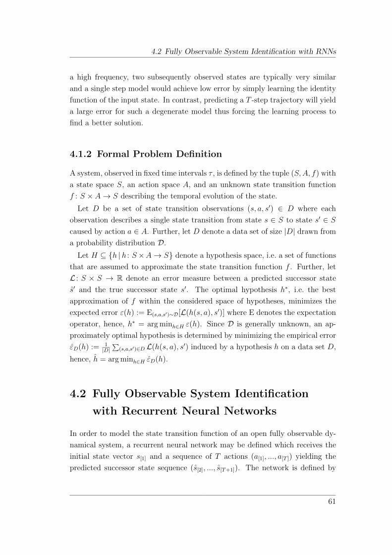
4.2 Fully Observable System Identification with RNNs
a high frequency, two subsequently observed states are typically very similar
and a single step model would achieve low error by simply learning the identity
function of the input state. In contrast, predicting a T -step trajectory will yield
a large error for such a degenerate model thus forcing the learning process to
find a better solution.
4.1.2 Formal Problem Definition
A system, observed in fixed time intervals τ , is defined by the tuple (S,A, f) with
a state space S, an action space A, and an unknown state transition function
f : S × A→ S describing the temporal evolution of the state.
Let D be a set of state transition observations (s, a, s′) ∈ D where each
observation describes a single state transition from state s ∈ S to state s′ ∈ Scaused by action a ∈ A. Further, let D denote a data set of size |D| drawn from
a probability distribution D.
Let H ⊆ h |h : S×A→ S denote a hypothesis space, i.e. a set of functions
that are assumed to approximate the state transition function f . Further, let
L : S × S → R denote an error measure between a predicted successor state
s′ and the true successor state s′. The optimal hypothesis h∗, i.e. the best
approximation of f within the considered space of hypotheses, minimizes the
expected error ε(h) := E(s,a,s′)∼D[L(h(s, a), s′)] where E denotes the expectation
operator, hence, h∗ = arg minh∈H ε(h). Since D is generally unknown, an ap-
proximately optimal hypothesis is determined by minimizing the empirical error
εD(h) := 1|D|∑
(s,a,s′)∈D L(h(s, a), s′) induced by a hypothesis h on a data set D,
hence, h = arg minh∈H εD(h).
4.2 Fully Observable System Identification
with Recurrent Neural Networks
In order to model the state transition function of an open fully observable dy-
namical system, a recurrent neural network may be defined which receives the
initial state vector s[1] and a sequence of T actions (a[1], ..., a[T ]) yielding the
predicted successor state sequence (s[2], ..., s[T+1]). The network is defined by
61
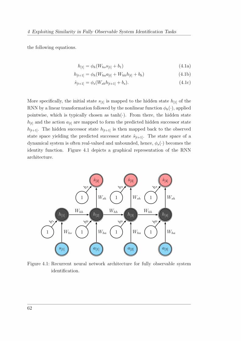
4 Exploiting Similarity in Fully Observable System Identification Tasks
the following equations.
h[1] = φh(Whss[1] + b1) (4.1a)
h[t+1] = φh(Whaa[t] +Whhh[t] + bh) (4.1b)
s[t+1] = φs(Wshh[t+1] + bs). (4.1c)
More specifically, the initial state s[1] is mapped to the hidden state h[1] of the
RNN by a linear transformation followed by the nonlinear function φh(·), applied
pointwise, which is typically chosen as tanh(·). From there, the hidden state
h[t] and the action a[t] are mapped to form the predicted hidden successor state
h[t+1]. The hidden successor state h[t+1] is then mapped back to the observed
state space yielding the predicted successor state s[t+1]. The state space of a
dynamical system is often real-valued and unbounded, hence, φs(·) becomes the
identity function. Figure 4.1 depicts a graphical representation of the RNN
architecture.
1 1 1 1
s[1] a[1] a[2] a[3]
1 1 1
h[1] h[2] h[3] h[4]
Wha Wha Wha
b 1 b h b h b h
Whs
Whh Whh Whh
s[2] s[3] s[4]
Wsh Wsh Wsh
b s b s b s
Figure 4.1: Recurrent neural network architecture for fully observable system
identification.
62
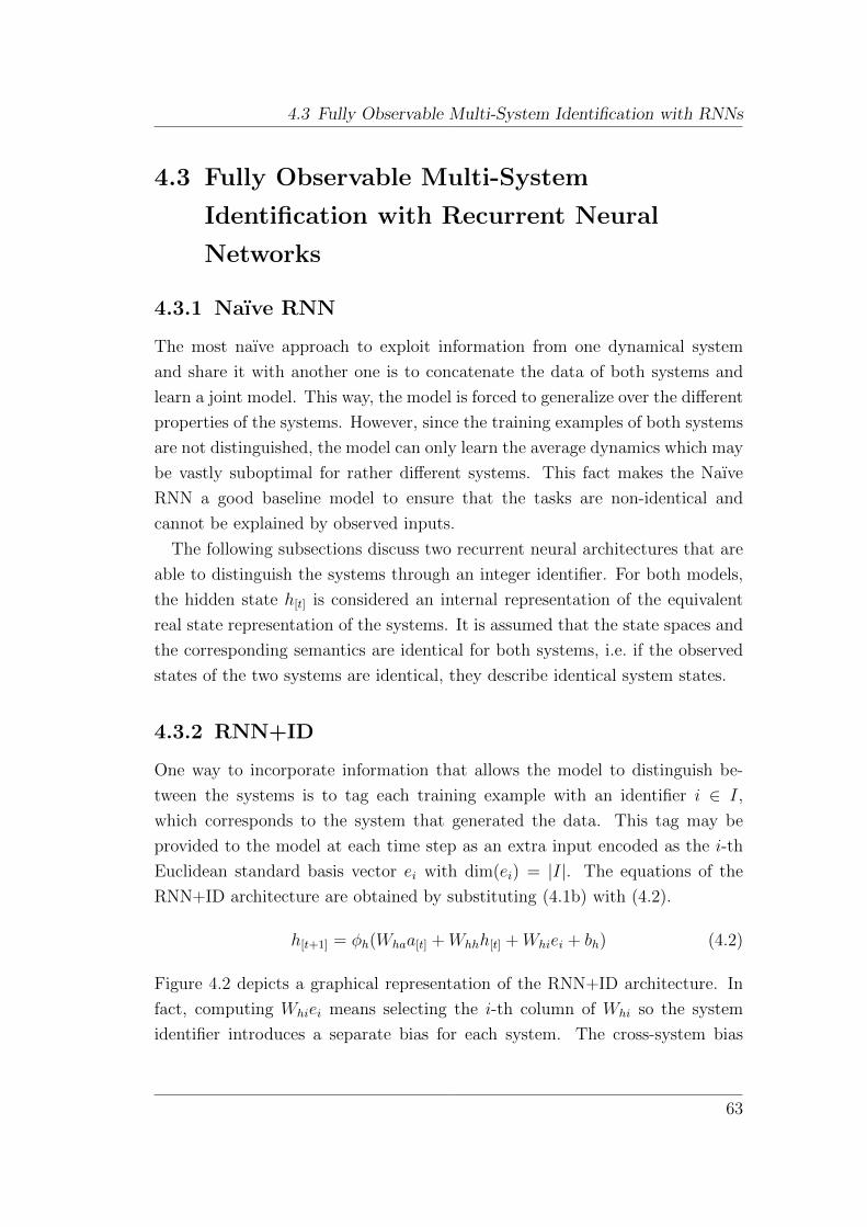
4.3 Fully Observable Multi-System Identification with RNNs
4.3 Fully Observable Multi-System
Identification with Recurrent Neural
Networks
4.3.1 Naıve RNN
The most naıve approach to exploit information from one dynamical system
and share it with another one is to concatenate the data of both systems and
learn a joint model. This way, the model is forced to generalize over the different
properties of the systems. However, since the training examples of both systems
are not distinguished, the model can only learn the average dynamics which may
be vastly suboptimal for rather different systems. This fact makes the Naıve
RNN a good baseline model to ensure that the tasks are non-identical and
cannot be explained by observed inputs.
The following subsections discuss two recurrent neural architectures that are
able to distinguish the systems through an integer identifier. For both models,
the hidden state h[t] is considered an internal representation of the equivalent
real state representation of the systems. It is assumed that the state spaces and
the corresponding semantics are identical for both systems, i.e. if the observed
states of the two systems are identical, they describe identical system states.
4.3.2 RNN+ID
One way to incorporate information that allows the model to distinguish be-
tween the systems is to tag each training example with an identifier i ∈ I,
which corresponds to the system that generated the data. This tag may be
provided to the model at each time step as an extra input encoded as the i-th
Euclidean standard basis vector ei with dim(ei) = |I|. The equations of the
RNN+ID architecture are obtained by substituting (4.1b) with (4.2).
h[t+1] = φh(Whaa[t] +Whhh[t] +Whiei + bh) (4.2)
Figure 4.2 depicts a graphical representation of the RNN+ID architecture. In
fact, computing Whiei means selecting the i-th column of Whi so the system
identifier introduces a separate bias for each system. The cross-system bias
63

4 Exploiting Similarity in Fully Observable System Identification Tasks
1
s[1] a[1] a[2] a[3]
1 1 1
h[1] h[2] h[3] h[4]
Wha Wha Wha
b 1
ei ei ei
Whi
Whi
Whi
Whs
Whh Whh Whh
s[2] s[3] s[4]
Wsh Wsh Wsh
b s b s b s
Figure 4.2: RNN+ID architecture for fully observable multi-system identifica-
tion.
bh and the specific biases accessed through Whiei can be absorbed into a new
system-specific bias ›Whiei = bh +Whiei. Thus, (4.2) can be rewritten as
h[t+1] = φh(Whaa[t] +Whhh[t] +›Whiei). (4.3)
4.3.3 FTRNN
The previous subsection showed that providing the network with a “one-hot”
encoded system identifier ei is in fact equivalent to learning a different hidden
layer bias ›Whiei for each system. The bias of a particular neuron determines
its activity threshold. Making the bias system-specific thus allows to learn a
different threshold for each system. However, the state evolution of a system is
predominantly determined by the matrix Whh, which models the state evolution
without external forces, and by the matrix Wha, which models the effect of an
external force applied to the system. Given that all systems share identical state
and action spaces, these two matrices should be made system-specific.
The idea of introducing third-order tensors as parameter matrices conditioned
on a categorical input, as described in Section 3.3.3, can be applied to the multi-
system identification problem. Following the arguments made above an immedi-
ate approach is to learn separate parameter matrices Whhiei and Whaiei for each
64

4.4 The Fully Observable Dual-Task Learning Problem
system where Whhi ∈ Rnh×nh×|I| and Whai ∈ Rnh×na×|I| are third-order tensors.
As argued in Section 3.3.3 learning separate parameter matrices for each system
has two major drawbacks regarding the number of parameters harming data effi-
ciency and regarding the independence of each parameter matrix which prevents
information sharing within the transformation. Decomposing the three-way ten-
sors Whhi and Whai according to PARAFAC yields the factored tensors of the
form
Whhiei ≈ Whfh diag(Wfhiei)Wfhh (4.4a)
Whaiei ≈ Whfa diag(Wfaiei)Wfaa (4.4b)
Substituting the matrices Whh and Wha by their corresponding factored tensors
yields the equations of the FTRNN by substituting (4.1b) with (4.5).
h[t+1] = φh(Whfa diag(Wfaiei)Wfaaa[t] +
Whfh diag(Wfhiei)Wfhhh[t] + bh)
(4.5)
Figure 4.3 depicts a graphical representation of the FTRNN architecture. Due to
the factored tensors, only nf parameters are specific to each system compared
to nunv parameters for independent parameter matrices Wvui. Their limited
degree of freedom forces the model to identify common structure among the
systems. This way, every system has its own set of transformations describing
the contributions of the previous hidden state and the current external force to
yield the current hidden state. However, these transformations are not indepen-
dent for each system since they are composed of two cross-system components
and one system-specific component.
4.4 The Fully Observable Dual-Task Learning
Problem
The fully observable dual-task learning problem addresses the task of learning
the state transition function of a little observed fully observable dynamical sys-
tem by utilizing data from a well-observed similar system. In order to achieve
this goal, the data of both systems are used to learn a joint model thereof such
that information is shared among the two systems. Typical applications of this
65
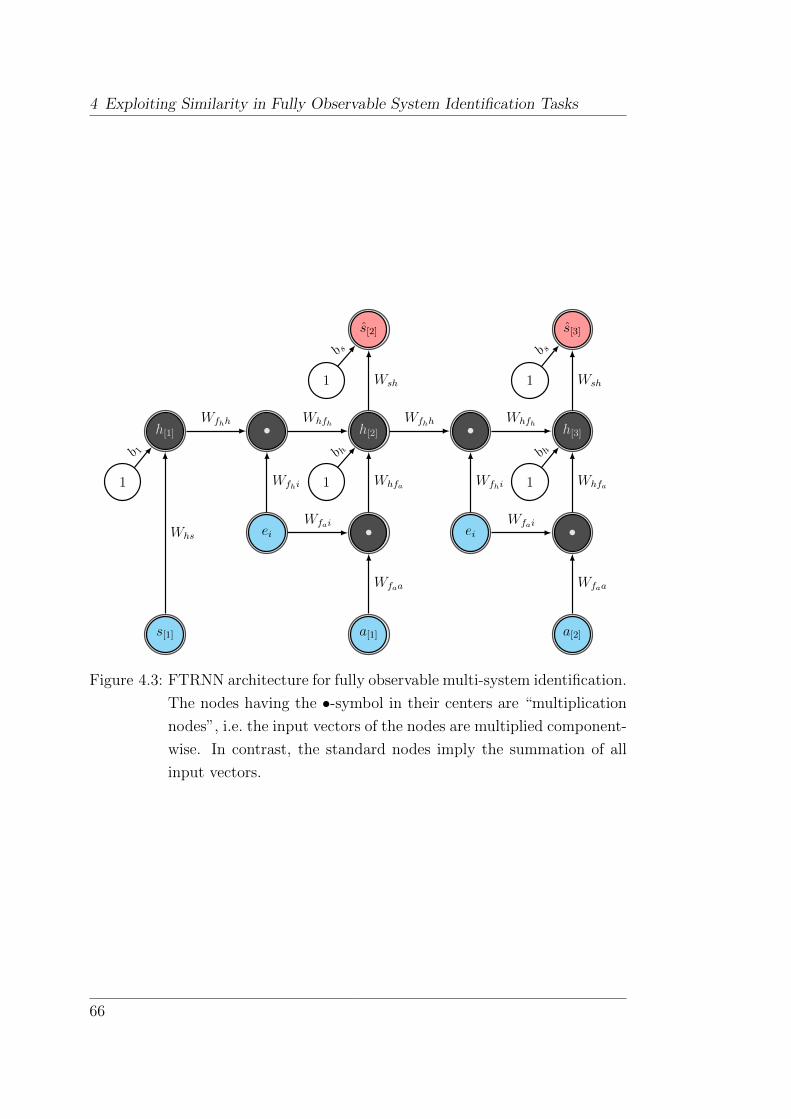
4 Exploiting Similarity in Fully Observable System Identification Tasks
1 1 1
s[1] a[1] a[2]
ei ei
1 1
h[1] • •
• •
h[2] h[3]
Wfai
Wfhi
Wfai
Wfhi
Wfaa
Whfa
Wfaa
Whfa
b 1 b h b hWhs
Wfhh Whfh Wfhh Whfh
s[2] s[3]
Wsh Wsh
b s b s
Figure 4.3: FTRNN architecture for fully observable multi-system identification.
The nodes having the •-symbol in their centers are “multiplication
nodes”, i.e. the input vectors of the nodes are multiplied component-
wise. In contrast, the standard nodes imply the summation of all
input vectors.
66
4.4 The Fully Observable Dual-Task Learning Problem
scenario are situations where a technical system undergoes maintenance pro-
cedures after a sufficiently long period of operation that cause the system to
change, or the deployment of a new instance whose data of observations are
augmented by those of a related system.
4.4.1 Problem Definition
Let I := 1, 2 denote a set of identifiers for fully observable deterministic
systems, which are observed in fixed time intervals τ and show similar dynamics.
A system is defined by the tuple (S,A, fi) with a state space S, an action space
A, and an unknown state transition function fi : S × A → S describing the
temporal evolution of the state.
Let Di be a set of state transition observations (i, s, a, s′) ∈ Di of the i-th
system where each observation describes a single state transition from state
s ∈ S to state s′ ∈ S caused by action a ∈ A. Further, let D =⋃i∈I Di denote
a data set of size |D| drawn from a probability distribution D.
Let H ⊆ h |h : S×A→ S denote a hypothesis space, i.e. a set of functions
that are assumed to approximate the state transition function fi. Further, let
L : S×S → R denote an error measure between a predicted successor state s′ and
the true successor state s′. The optimal hypothesis h∗i , i.e. the best approxima-
tion of fi within the considered space of hypotheses, minimizes the conditional
expected error εi(h) := E(j,s,a,s′)∼D[L(h(s, a), s′) | j = i] where E denotes the
expectation operator, hence, h∗i = arg minh∈H εi(h). Since D is generally un-
known, an approximately optimal hypothesis is determined by minimizing the
empirical error εD(h) := 1|D|∑
(·,s,a,s′)∈D L(h(s, a), s′) induced by a hypothesis h
on a data set D, hence, hi = arg minh∈H εDi(h).
Given sufficient data D1, it is expected that |ε1(h1) − ε1(h∗1)| ≤ ε for some
small positive ε. In contrast, assuming the amount of data D2 is insufficient,
|ε2(h2) − ε2(h∗2)| ε and h2 may be useless. The problem addressed in this
section is to develop and assess methods that yield a better hypothesis of the
insufficiently observed system through dual-task learning in order to utilize aux-
iliary information from D1 as prior knowledge of the transition function f2.
Therefore, the hypothesis space and the empirical error are redefined as fol-
lows. Let H ′ ⊆ h |h : I × S × A → S denote an extended hypothesis space,
which includes the system identifier into the product space of arguments and
67
4 Exploiting Similarity in Fully Observable System Identification Tasks
thus approximates both transition functions by a single function. Further, let
ε′D(h) := 1|D|∑
(i,s,a,s′)∈D wiL(h(i, s, a), s′) denote the empirical error of a hy-
pothesis h ∈ H ′ with the system-specific error weight wi. If the the empirically
optimal hypothesis h′ = arg minh∈H′ ε′D(h) (D =
⋃i∈I Di) yields a smaller ex-
pected error than h2, i.e. ε2(h′2) < ε2(h2) with h′2(s, a) := h′(2, s, a), information
from the well observed system is successfully utilized in the hypothesis search
to find a better hypothesis of f2 despite few data.
4.4.2 Experiments
In order to assess the effectiveness of the FTRNN model in comparison with
the competing models, experiments were conducted using the frictionless cart-
pole (see Section 2.8.1) and mountain car (see Section 2.8.2) simulations. For
each simulation, two instances with non-identical but similar state transition
functions were configured. The data sets D1 and D2 were obtained by observing
the state transitions (i, s, a, s′) along a trajectory of 500 actions (a[1], ..., a[500])
defined by the equations
a[0] = 0 (4.6a)
a[t] ∼ U(−1, 1) (4.6b)
a[t] = max(−1,min(1, a[t−1] + a[t])). (4.6c)
with U being the uniform distribution. These equations describe a random walk
of actions clipped to the domain of the action space. After every 500 steps, the
simulation was reset to its initial state. The examples used to train and evalu-
ate the models were generated by extracting T -step windows of the sequences of
observations. In order to decorrelate examples of the training, validation, and
generalization data sets, the block validation method discussed in Section 2.3.3
was used. D1 consisted of 15 000 examples (i = 1, s[1], a[1], ..., s[T ], a[T ], s[T+1])
and was split into a training set D1,T containing 10 000 examples and a val-
idation set D1,V sized 5000. The data set D2 was obtained the same way,
however, training and validation set sizes were reduced to 10000, 5000, ..., 156and 5000, 2500, ..., 78 respectively throughout the experiments. Experiments
were conducted on two simulations in order to (i) compare the model error
as a function of D2,T and D2,V, and (ii) assess whether D2,T and D2,V should
be upsampled to match the sizes of D1,T and D1,V or not. The loss function
68
4.4 The Fully Observable Dual-Task Learning Problem
for training was chosen to be the mean squared error (MSE) between the pre-
dicted and the true successor state sequence, i.e. L(s[2], ..., s[T+1], s[2], ..., s[T+1]) =12
∑Tt=1 ‖s[t+1] − s[t+1]‖2
2. An alternative choice is the “ln cosh” loss function in
case outliers are a concern (Neuneier & Zimmermann, 1998). To evaluate the
model performances, the average MSE per time step per output component was
used, i.e. Ltest = 1T dim(s)
L.
Learning the state transition function of the differently configured systems
cannot be solved through mere generalization because the quantities that invoke
the different dynamical behavior are hidden. The only information that allows
to distinguish the systems is a categorical system identifier. Thus, the hidden
quantities need to be inferred from observations making the problem a dual-task
learning problem rather than a problem of generalization.
Cart-Pole
Two cart-pole instances (CP1 and CP2) were configured to have the pole lengths
0.5 and 1.0, and the pole masses 0.05 and 0.1, respectively. Figure 4.4 depicts
the performance of the best-of-five model (determined by the lowest error on
D1,V ∪ D2,V with |D1,V| = 5000 and |D2,V| = 12|D2,T|) with T = 10 evaluated
on D2,G with |D2,G| = 100 000. In each run, the initial model parameters were
sampled at random. For all networks, the hidden state dimension was set to
nh = 10. The hyperparameters of the FTRNN were set to nfh = nh and nfa = 1.
The simple RNN model was only trained on data from CP2. The other models,
i.e. the Naıve RNN, RNN+ID and FTRNN, were trained on the concatenated
data set D1 ∪ D2. The model parameters were optimized using Hessian-Free
optimization with the structural damping coefficient (see Section 2.4.2) set to
µsd = 0.1, a maximum number of 10 000 updates, at most 150 conjugate gradient
(CG) iterations using all training examples to compute the gradient, and a
random subset of the training data set sized 5000 to estimate the local curvature
of the error surface. In addition, an early stopping procedure with a patience
of 50 updates was used to reduce overfitting.
The first set of experiments, whose results are depicted in Figure 4.4a, com-
pared the errors of the different models provided that D2,T and D2,V were up-
sampled such that |D2,T| = |D1,T| and |D2,V| = |D1,V|. As a result, the simple
RNN performed well for |D2,T| ∈ 1250, 2500, 5000, 10 000 but degraded rapidly
69
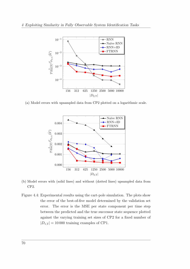
4 Exploiting Similarity in Fully Observable System Identification Tasks
156 312 625 1250 2500 5000 10000
10−4
10−3
10−2
10−1
|D2,T|
1T
dim
(S)ε′ D
2,G
(h′ )
RNNNaıve RNNRNN+IDFTRNN
(a) Model errors with upsampled data from CP2 plotted on a logarithmic scale.
156 312 625 1250 2500 5000 10000
0.000
0.001
0.002
0.003
0.004
|D2,T|
1T
dim
(S)ε′ D
2,G
(h′ )
Naıve RNNRNN+IDFTRNN
(b) Model errors with (solid lines) and without (dotted lines) upsampled data from
CP2.
Figure 4.4: Experimental results using the cart-pole simulation. The plots show
the error of the best-of-five model determined by the validation set
error. The error is the MSE per state component per time step
between the predicted and the true successor state sequence plotted
against the varying training set sizes of CP2 for a fixed number of
|D1,T| = 10 000 training examples of CP1.
70
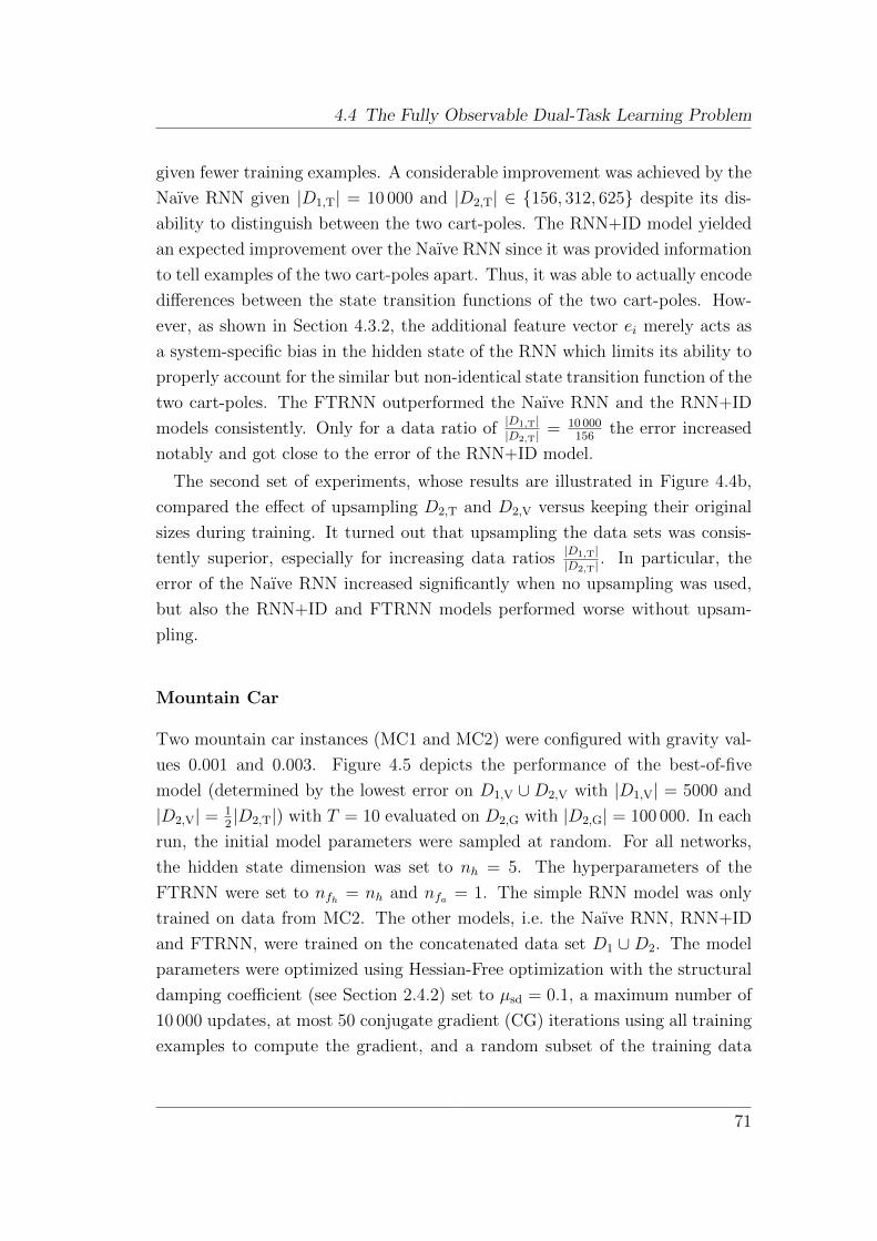
4.4 The Fully Observable Dual-Task Learning Problem
given fewer training examples. A considerable improvement was achieved by the
Naıve RNN given |D1,T| = 10 000 and |D2,T| ∈ 156, 312, 625 despite its dis-
ability to distinguish between the two cart-poles. The RNN+ID model yielded
an expected improvement over the Naıve RNN since it was provided information
to tell examples of the two cart-poles apart. Thus, it was able to actually encode
differences between the state transition functions of the two cart-poles. How-
ever, as shown in Section 4.3.2, the additional feature vector ei merely acts as
a system-specific bias in the hidden state of the RNN which limits its ability to
properly account for the similar but non-identical state transition function of the
two cart-poles. The FTRNN outperformed the Naıve RNN and the RNN+ID
models consistently. Only for a data ratio of|D1,T||D2,T| = 10 000
156the error increased
notably and got close to the error of the RNN+ID model.
The second set of experiments, whose results are illustrated in Figure 4.4b,
compared the effect of upsampling D2,T and D2,V versus keeping their original
sizes during training. It turned out that upsampling the data sets was consis-
tently superior, especially for increasing data ratios|D1,T||D2,T| . In particular, the
error of the Naıve RNN increased significantly when no upsampling was used,
but also the RNN+ID and FTRNN models performed worse without upsam-
pling.
Mountain Car
Two mountain car instances (MC1 and MC2) were configured with gravity val-
ues 0.001 and 0.003. Figure 4.5 depicts the performance of the best-of-five
model (determined by the lowest error on D1,V ∪D2,V with |D1,V| = 5000 and
|D2,V| = 12|D2,T|) with T = 10 evaluated on D2,G with |D2,G| = 100 000. In each
run, the initial model parameters were sampled at random. For all networks,
the hidden state dimension was set to nh = 5. The hyperparameters of the
FTRNN were set to nfh = nh and nfa = 1. The simple RNN model was only
trained on data from MC2. The other models, i.e. the Naıve RNN, RNN+ID
and FTRNN, were trained on the concatenated data set D1 ∪ D2. The model
parameters were optimized using Hessian-Free optimization with the structural
damping coefficient (see Section 2.4.2) set to µsd = 0.1, a maximum number of
10 000 updates, at most 50 conjugate gradient (CG) iterations using all training
examples to compute the gradient, and a random subset of the training data
71
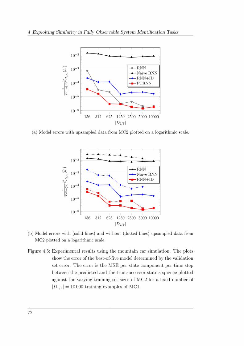
4 Exploiting Similarity in Fully Observable System Identification Tasks
156 312 625 1250 2500 5000 10000
10−6
10−5
10−4
10−3
10−2
|D2,T|
1T
dim
(S)ε′ D
2,G
(h′ ) RNN
Naıve RNNRNN+IDFTRNN
(a) Model errors with upsampled data from MC2 plotted on a logarithmic scale.
156 312 625 1250 2500 5000 10000
10−6
10−5
10−4
10−3
10−2
|D2,T|
1T
dim
(S)ε′ D
2,G
(h′ ) RNN
Naıve RNNRNN+ID
(b) Model errors with (solid lines) and without (dotted lines) upsampled data from
MC2 plotted on a logarithmic scale.
Figure 4.5: Experimental results using the mountain car simulation. The plots
show the error of the best-of-five model determined by the validation
set error. The error is the MSE per state component per time step
between the predicted and the true successor state sequence plotted
against the varying training set sizes of MC2 for a fixed number of
|D1,T| = 10 000 training examples of MC1.
72
4.4 The Fully Observable Dual-Task Learning Problem
set sized 5000 to estimate the local curvature of the error surface. In addition,
an early stopping procedure with a patience of 50 updates was used to reduce
overfitting.
The first set of experiments, whose results are depicted in Figure 4.5a, com-
pared the errors of the different models provided that D2,T and D2,V were up-
sampled such that |D2,T| = |D1,T| and |D2,V| = |D1,V|. As a result, the simple
RNN performed well in general, but its error increased for an increasing data
ratio|D1,T||D2,T| . In contrast to the cart-pole experiments, the Naıve RNN performed
orders of magnitude worse than all other models. The RNN+ID modeled the
state transition function of MC2 considerably more accurately than the Naıve
RNN, but it was almost consistently worse than the simple RNN. It only out-
performed the simple RNN for |D2,T| = 156. The FTRNN again performed
consistently best by a significant margin in comparison with the other models.
Surprisingly, it even achieved a smaller error than the simple RNN for small
data ratios|D1,T||D2,T| . For |D2,T| = 156 its error was more than an order of magni-
tude smaller than the error of the simple RNN. Upon further investigation, the
RNN turned out to be slightly underfitting given many training examples.
The second set of experiments, whose results are illustrated in Figure 4.5b,
compared the effect of upsampling D2,T and D2,V versus keeping their original
sizes during training. The observations made during the mountain car experi-
ments were qualitatively consistent with those of the cart-pole experiments. For
all models, upsampling the data yielded smaller model errors.
4.4.3 Discussion
The problem class of modeling the state transition function of a dynamical sys-
tem from few observations by utilizing auxiliary data from a similar system was
introduced, motivated and formalized. For this purpose, the Factored Tensor
Recurrent Neural Network (FTRNN) architecture was presented, discussed, and
its effectiveness was assessed in a series of experiments using the cart-pole and
mountain car simulations. The FTRNN was compared with two variants of
recurrent neural networks which implement different approaches of information
sharing in a dual-task learning setting. In addition, it was also investigated
whether the few data of the target system should be upsampled to match the
amount of data of the source system, thus, giving equal weight to the source
73

4 Exploiting Similarity in Fully Observable System Identification Tasks
and target systems in the training objective. As a result, the FTRNN turned
out consistently and significantly superior to the compared methods on both
simulations across the range of considered data ratios. Further, the experi-
ments showed that matching the data set sizes of the two system by means of
upsampling yielded a smaller error for all models.
4.5 The Fully Observable Dual-Task Learning
Problem with Regularization
Given only few training examples from the target system the parameters of
its corresponding model may converge to unfavorable values as the available
information is insufficient. To address this problem, a regularization term, which
extends the optimization objective of the FTRNN model, is presented preventing
the model of the target system from diverging from the model of the source
system. The latter is assumed to be trustworthy because its parameters are
fitted to sufficiently many and rich data. Given the prior assumption of the
systems’ similarity the regularization acts as a similarity enforcing constraint
applied to the model parameters.
4.5.1 Problem Definition
The problem definition of this section extends the problem definition of Sec-
tion 4.4.1. The empirical error ε′D(h) := 1|D|∑
(i,s,a,s′)∈D wiL(h(i, s, a), s′) of a
hypothesis h ∈ H ′ is extended by a regularization term that constrains the
choice of hypotheses in a way that the prior assumption of the two system be-
ing similar is further strengthened. The regularized empirical error ε′D,λ(h) :=1|D|∑
(i,s,a,s′)∈D wiL(h(i, s, a), s′) + λ||h|| is obtained through an additional ad-
ditive term. If the empirically optimal hypothesis h′λ = arg minh∈H′ ε′D,λ(h)
(D =⋃i∈I Di) yields a smaller expected error than h′ and h2, i.e. ε2(h′2,λ) <
ε2(h′2) < ε2(h2) with h′2(·, ·) := h′(2, ·, ·), the regularization method improves
the utilization of information from the well observed system in the hypothesis
search to find a better hypothesis of f2 despite few data.
74

4.5 The Fully Observable Dual-Task Learning Problem with Regularization
4.5.2 Regularization
Let Ω: Rnf×|I| → R+ be a regularization function that maps a matrix, whose
columns hold the system-specific parameters of each system, to a non-negative
real-valued regularization cost. The function asymmetrically penalizes the Eu-
clidean distance between two columns of the parameter matrix, i.e. the system-
specific parameters of the target system are tied to those of the source system but
not vice versa. In the limit of a strong regularization coefficient, the regularized
FTRNN objective makes the FTRNN and Naıve RNN equivalent because the
system-specific parameters are forced to be equal. The regularization function
is defined as
Ω(Wfi) = ‖const(Wfi)e1 −Wfie2‖22 (4.7)
where const(·) is a function whose argument is made constant with respect to
differentiation, i.e.∂const(Wfi)
∂Wfi= 0. The error function, minimized with respect
to θ = θcross ∪ θspecific with θcross = Whs, b1,Wfaa,Whfa ,Wfhh,Whfh , bh,Wsh, bsand θspecific = Wfai,Wfhi, is given by
E(θ;λa, λh) = εD(hFTRNN,θ) + λaΩ(Wfai) + λhΩ(Wfhi). (4.8)
Thus, the optimal parameters θ∗ are found as follows:
θ∗ = arg minθ
E(θ, λa, λh) (4.9)
The hyperparameters λa ≥ 0 and λh ≥ 0 are determined via cross-validation.
There are two reasons for constraining the effect of the regularization to the
target system. First, the system-specific parameters of the source system are
assumed to be well determined by the data. Hence, there is no need to exploit
information from the target system. In fact, the little and possibly incomplete
information about the target system might even corrupt the parameters of the
source system. Second, the cross-system parameters adjust according to the
dual-task learning objective which is the minimization of (4.8). Since the data
of the target system are considered insufficient and likely incomplete, minimizing
the prediction error on the training data is likely to generalize poorly for this
system. Thus, not only the system-specific parameters of the target system but
also the cross-system parameters may adjust unfavorably. By constraining the
system-specific parameters of the target system to remain similar to those of
75
4 Exploiting Similarity in Fully Observable System Identification Tasks
the source system, the cross-system parameters are less likely to be affected
by incomplete information about the target system. Note, however, that the
regularization nevertheless affects the system-specific parameters of the source
system implicitly via the cross-system parameters, but the effect should be much
more lenient.
4.5.3 Experiments
Experiments were conducted on the cart-pole (see Section 2.8.1) and mountain
car (see Section 2.8.2) simulations. For each simulation two different instances
of the respective systems were instantiated. One of the two systems was desig-
nated the source system from which sufficient data were available while the other
system was designated the target system which had only been observed insuffi-
ciently in order to learn an accurate model thereof. The experiments especially
focused on large data ratios between the source and target systems assessing
the effectiveness of the regularization technique in such situations. Regulariza-
tion coefficients in an appropriate range were compared across a range of data
ratios. The training, validation, and test data sets were created using the block
validation method (see Section 2.3.3).
Cart-Pole
Sequences of 1000 actions a[t] ∼ U(−1, 1) were applied to the cart-pole every τ =
0.02 s for which the resulting state transitions were observed. After completing
a sequence, the simulation was reset to its initial state. Two different cart-poles,
whose configurations varied in terms of the pole length lpole and pole mass mpole,
were observed. The two cart-poles were configured by setting lpole ∈ 0.5, 1.0and mpole = 0.1lpole. For cart-pole 1 (CP1), a training data set with 10 000 and
a validation data set with 5000 examples were created. For cart-pole 2 (CP2),
various training data sets sized 10 000, 5000, ..., 625 and validation data sets
sized 5000, 2500, ..., 312 were created. During training, the two training and
validation data sets were concatenated and the data of CP2 were upsampled
to be equal in size with those of CP1. To test the performance of the models,
a generalization data set for CP2 sized 30 000 was created. The FTRNN was
configured using nh = nfh = 10, nfa = 2 and T = 10. The regularization
strength was set to λ = λa = λh ∈ 10−4, 10−3, 10−2. The maximum number
76

4.5 The Fully Observable Dual-Task Learning Problem with Regularization
of parameter updates was set to 10 000. The number of conjugate gradient (CG)
iterations per update was limited to 150. The gradient was computed using the
full training set and the curvature was estimated using 5000 examples.
Figure 4.6 depicts the performance of the FTRNN with and without regular-
ization. The performance metric is the median of five runs of the average MSE
625 1250 2500 5000 1000010−4
10−3
73%
|DT,2|
1T
dim
(S)ε D
G,2(h)
FTRNN (λ = 0) FTRNN (λ = 10−4)
FTRNN (λ = 10−3) FTRNN (λ = 10−2)
Figure 4.6: Experimental results of the cart-pole simulation. The average MSE
per state component per time step of the predicted and the true
successor state sequence is plotted against the varying training set
size of CP2 for |D1,T| = 10 000 training examples of CP1.
per state component per predicted time step. At the beginning of each run, a
new parameter initialization was sampled at random.
The experiments on the cart-pole simulation revealed superior performance of
the regularized FTRNN over the plain FTRNN for |D2,T| = 625. The smallest
error was obtained by setting λ = 10−2. A large coefficient reduced the error for
|D2,T| = 625 but increased it for |D2,T| ∈ 1250, 2500, 5000, 10 000 compared
to the plain FTRNN was observed. This observation is plausible because the
regularization constrains the parameters of CP2 to be close to those of CP1.
When enough data of CP2 were available, this heuristic was likely invalid and
harmful to the model performance. However, given only few data of CP2, it
guided the parameters towards a better optimum.
77

4 Exploiting Similarity in Fully Observable System Identification Tasks
Mountain Car
Sequences of 500 actions (a[1], ..., a[500]), computed by the equations
a[0] = 0 (4.10a)
a[t] ∼ U(−1, 1) (4.10b)
a[t] = max(−1,min(1, a[t−1] + a[t])), (4.10c)
were applied to the mountain car. After completing a sequence, the simulation
was reset to its initial state. Two mountain cars, whose configurations differed
in terms of the gravity g ∈ 0.0005, 0.0009, were observed. For mountain car
1 (MC1), a training data set with 10 000 and a validation data set with 5000
examples were created. For mountain car 2 (MC2), various training data sets
sized 10 000, 5000, ..., 156 and validation data sets sized 5000, 2500, ..., 78were created. During training, the two training and validation data sets were
concatenated and the data of MC2 were upsampled to be equal in size with
those of MC1. To test the performance of the models, a generalization data
set for MC2 sized 100 000 was created. The FTRNN was configured using
nh = nfh = 10, nfa = 2 and T = 10. The regularization strength was set to
λ = λa = λh ∈ 10−3, 10−2, 10−1. The maximum number of parameter updates
was set to 5000. The number of conjugate gradient (CG) iterations per update
was limited to 100. The gradient was computed using the full training set and
the curvature was estimated using 10 000 examples.
Figure 4.7 depicts the performance of the FTRNN with and without regular-
ization. The performance metric is the average MSE per state component per
predicted time step of the best model among five runs, determined by the val-
idation set error. At the beginning of each run, a new parameter initialization
was sampled at random.
The experiments on the mountain car simulation revealed superior perfor-
mance of the regularized FTRNN over the plain FTRNN for |DT,2| ∈ 312, 156.Given |DT,2| = 312 and for λ = 10−3, a relative error reduction of approxi-
mately 76 % compared to the plain FTRNN. For |D2,T| = 156 and λ = 10−2,
the regularization yielded a relative improvement of approximately 83 %. Sim-
ilar to the observations made in the cart-pole experiments, the regulariza-
tion reduced the error for |D2,T| ∈ 312, 156 but tended to increase it for
|D2,T| ∈ 625, 1250, ..., 10 000.
78
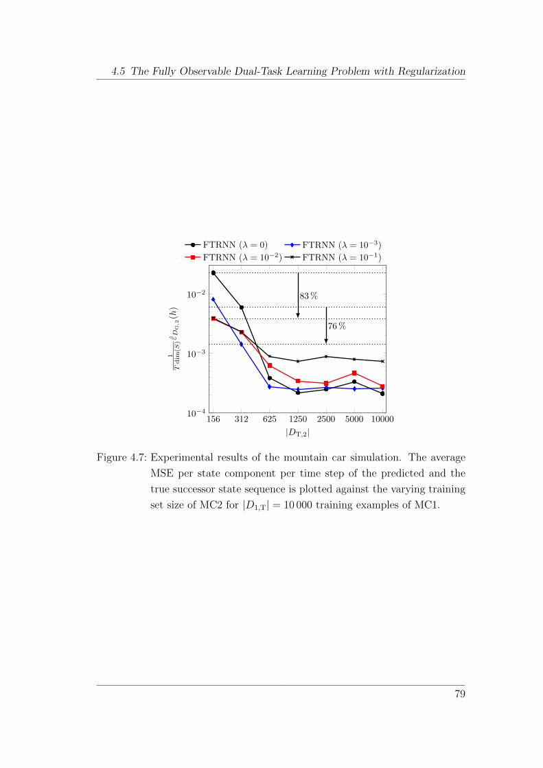
4.5 The Fully Observable Dual-Task Learning Problem with Regularization
156 312 625 1250 2500 5000 1000010−4
10−3
10−2 83%
76%
|DT,2|
1T
dim
(S)ε D
G,2(h)
FTRNN (λ = 0) FTRNN (λ = 10−3)
FTRNN (λ = 10−2) FTRNN (λ = 10−1)
Figure 4.7: Experimental results of the mountain car simulation. The average
MSE per state component per time step of the predicted and the
true successor state sequence is plotted against the varying training
set size of MC2 for |D1,T| = 10 000 training examples of MC1.
79
4 Exploiting Similarity in Fully Observable System Identification Tasks
4.5.4 Discussion
A regularization technique for the Factored Tensor Recurrent Neural Network
(FTRNN) to learn the dynamics of an insufficiently observed target system by
exploiting its similarity with a well observed source system in a dual-task learn-
ing approach was presented. The FTRNN disentangles cross-system properties
from peculiarities allowing to share knowledge efficiently among the systems.
When information from the target system was insufficient in order to learn an
accurate FTRNN model, it was discovered that especially the system-specific
parameters converged to unfavorable values. This section addressed the prob-
lem through regularization which penalizes dissimilarities between the system-
specific parameters of the source and target system asymmetrically such that
the system-specific parameters of the target system were penalized for diverg-
ing from those of the source system but not vice versa. The effectiveness of
this approach was demonstrated on the cart-pole and mountain car simulations
achieving significantly lower errors using the regularized FTRNN compared to
the plain FTRNN.
4.6 The Fully Observable Transfer Learning
Problem
In this section, an efficient transfer learning approach based on recurrent neural
networks with factored tensor components is introduced. The goal is to identify
a target system based on few observations by exploiting its similarity with mul-
tiple well observed source systems. First, a joint model of the source systems is
trained which encodes cross-system properties and system-specific characteris-
tics into disjoint subsets of the model parameters. Second, a model of the target
system is obtained by merely fitting the system-specific parameters to the few
data of the target system while the cross-system parameters remain fixed. The
benefits of this approach are manifold. First, once a joint model of the source
systems is learned, knowledge transfer to a target system is fast, i.e. parameter
optimization converges within seconds, whereas learning the parameters of an
RNN from scratch can take many hours or even days. Second, this approach is
data-efficient with respect to the number of required target system observations
80
4.6 The Fully Observable Transfer Learning Problem
because the general dynamics of the source systems were identified based on
plenty of observations. Third, this method alleviates tedious hyperparameter
tuning, especially for the case of few available target system observations, since
the number of system-specific parameters is small and their effect on the overall
model is highly constrained. Fourth, the model complexity of the approach with
respect to a single system is identical to the complexity of the corresponding
simple RNN. Therefore, its evaluation time for a new system is the same.
The following subsections formalize the fully observable transfer learning
problem and present experimental results of the proposed neural architecture
with alternative approaches on data obtained from the cart-pole and mountain
car simulations. The empirical results are discussed and conclusions are drawn.
4.6.1 Formal Problem Definition
Let I := 1, 2, 3, ... denote the set of identifiers for fully observable deterministic
systems, which are observed in fixed time intervals τ and show similar dynamics.
A system is defined by the tuple (S,A, fi) with a state space S, an action space
A, and an unknown state transition function fi : S × A → S describing the
temporal evolution of the state.
Let Di be a set of state transition observations (i, s, a, s′) ∈ Di of the i-th
system where each observation describes a single state transition from state
s ∈ S to state s′ ∈ S caused by action a ∈ A. Further, let D =⋃i∈I Di denote
a data set of size |D| drawn from a probability distribution D.
Let H ⊆ h |h : S×A→ S denote a hypothesis space, i.e. a set of functions
that are assumed to approximate the state transition function fi. Further, let
L : S×S → R denote an error measure between a predicted successor state s′ and
the true successor state s′. The optimal hypothesis h∗i , i.e. the best approxima-
tion of fi within the considered space of hypotheses, minimizes the conditional
expected error εi(h) := E(j,s,a,s′)∼D[L(h(s, a), s′) | j = i] where E denotes the
expectation operator, hence, h∗i = arg minh∈H εi(h). Since D is generally un-
known, an approximately optimal hypothesis is determined by minimizing the
empirical error εD(h) := 1|D|∑
(·,s,a,s′)∈D L(h(s, a), s′) induced by a hypothesis h
on a data set D, hence, hi = arg minh∈H εDi(h).
Let the set of system identifiers I refer to |I| − 1 source systems with plenty
of available data and one target system with only few data, i.e. |D|I|| |Di| for
81
4 Exploiting Similarity in Fully Observable System Identification Tasks
all i ∈ I \ |I|. Given the sufficient amount of data from the source systems
i ∈ I\|I|, |εi(hi)−εi(h∗i )| ≤ ε for some small positive ε. In contrast, given only
few data D|I| from the target system, |ε|I|(h|I|)− ε|I|(h∗|I|)| ε and h|I| may be
useless. The problem addressed in this section is to develop and assess methods
that yield a better hypothesis of the insufficiently observed system through
transfer learning in order to utilize auxiliary information from⋃i∈I\|I|Di as
prior knowledge of the transition function f|I|.
Therefore, the hypothesis space and the empirical error are redefined as fol-
lows. Let H ′ ⊆ h |h : I × S × A → S denote an extended hypothesis space,
which includes the system identifier into the product space of arguments and
thus approximates both transition functions by a single function. Further, let
ε′D(h) := 1|D|∑
(i,s,a,s′)∈D wiL(h(i, s, a), s′) denote the empirical error of a hypoth-
esis h ∈ H ′ with the system-specific error weight wi. If the empirically optimal
hypothesis h′ = arg minh∈H′ ε′D(h) (D =
⋃i∈I Di) yields a smaller expected error
than h|I|, i.e. ε|I|(h′|I|) < ε|I|(h|I|) with h′|I|(s, a) := h′(|I|, s, a), information from
the well observed system was successfully utilized in the hypothesis search to
find a better hypothesis of f|I| despite few data.
4.6.2 Experiments
Experiments were conducted using two standard simulations: the frictionless
cart-pole (see Section 2.8.1) and mountain car (see Section 2.8.2) simulations
both modified from their originals to support continuous actions. For each
simulation, five different source system instances were labeled 1, ..., 5 and
various other instances were labeled 6. The properties of the target systems
were configured at random according to some distribution. Each system was
observed under a random policy to obtain data for training and evaluation. In
order to decorrelate the examples of the training, validation and generalization
data sets, the block validation method discussed in Section 2.3.3 was applied.
Let Di,T denote the set of training examples, let Di,V be the validation set
and Di,G be the generalization set for system i ∈ 1, ..., 6. The data set sizes
of the target system were assumed to be much smaller than those of the source
systems, i.e. D6,T Di,T and D6,V Di,V for i ∈ 1, ..., 5. Each example was
represented as a tuple (i, s[1], ..., s[T+1], a[1], ..., a[T ]).
The following protocol was used for all experiments:
82

4.6 The Fully Observable Transfer Learning Problem
1. Simple RNN models were trained for all source systems with different data
set sizes to roughly determine the amount of training examples needed to
learn good and poor models of the state transition function.
2. Data set sizes were chosen according to the results of step 1. The Naıve
RNN, RNN+ID, and FTRNN models were trained on the concatenated
training sets of all source systems (plenty of data) until the validation
error, evaluated on the concatenated validation sets, stopped improving
for at least 50 parameter updates. In addition, simple RNN models were
trained for all target systems (few data) using their corresponding data
sets until the validation error stopped improving for at least 50 parameter
updates. This process was repeated five times, each time with a fresh
random initialization of the model parameters. Among the five runs, the
best set of parameters was picked according to the validation set error.
3. For the RNN+ID and FTRNN architecture, the cross-system parameters
were transferred to the target system model by initializing its cross-system
parameters with the parameters of the source systems’ model. The system-
specific parameters of the target system model were initialized as the aver-
age of the system-specific parameters of the source systems’ model. When
training the target system model, only the system-specific parameters were
fitted to the training data of the target system until the validation set error
stopped improving for at least 50 parameter updates. The cross-system
parameters were considered constant with respect to the optimization ob-
jective. This process was repeated for all target systems.
4. Finally, the errors of the RNN, Naıve RNN, RNN+ID, and FTRNN models
were evaluated on the generalization data sets of the target systems. For
the RNN+ID and FTRNN models, the system-specific parameters of the
respective target system model, which had been obtained in the previous
step, were used.
83

4 Exploiting Similarity in Fully Observable System Identification Tasks
Cart-Pole
A cart-pole was observed every τ = 0.02 s for sequences of 500 actions (a[1], ..., a[500])
computed by the equations
a[0] = 0 (4.11a)
a[t] ∼ U(−1, 1) (4.11b)
a[t] = max(−1,min(1, a[t−1] + a[t])). (4.11c)
After every 500 steps, the simulation was reset to its initial state. Differ-
ent cart-poles, whose configurations varied in terms of the pole length lpole
and pole mass mpole, were observed. Each cart-pole i ∈ I \ |I| was con-
figured by setting lpole ∈ 0.5, 0.6, 0.7, 0.8, 0.9 and mpole = 0.1lpole, and data
sets of size |Di,T| = 10 000, |Di,V| = 5000, and |Di,G| = 100 000 were cre-
ated. Further, various other cart-pole configurations were created by sampling
lpole ∼ U(0.3, 1.1). The corresponding data sets were sized |D6,T| = 156,
|D6,V| = 78 and |D6,G| = 100 000. The RNNs were configured as follows:
nh = nfh = 20, nfa = 1, T = 10. The parameters were fitted to the data using
Hessian-Free optimization with structural damping (see Section 2.4.2 for details)
with the structural damping coefficient µsd = 0.1 and the initial Levenberg-
Marquardt coefficient λLM = 1.0. The gradient of the optimization objective
with respect to the parameters was computed using 10 000 examples selected at
random without replacement from the training data set. During the conjugate
gradient (CG) iterations, 5000 examples from the training data set were selected
at random without replacement. The CG method ran for at most 150 iterations
per update. Further, at most 10 000 parameter updates were allowed. These
hyperparameters were not exhaustively cross-validated, but they were found to
work well based on testing several different settings.
Figure 4.8 depicts the results of the experiments conducted using the cart-pole
simulation.
Figure 4.8a shows the similarity of the cart-poles labeled 1, ..., 5 by evalu-
ating every RNN model on every cart-pole configuration. Clearly, the models
were accurate when trained and evaluated on the same configuration, but the
accuracy decreased notably when a model was trained on a data from a partic-
ular cart-pole configuration and evaluated on data from another one. Further,
increasing the difference between the pole lengths and pole masses of two cart-
84

4.6 The Fully Observable Transfer Learning Problem
0 1 2 3 4
Evaluated on mountain car x
0
1
2
3
4
Tra
ined
onm
ounta
inca
ry
10−5
10−4
10−3
(a) Similarity of the source systems
0.4 0.6 0.8 110−5
10−4
10−3
10−2
10−1
100
lpole = 0.1mpole
1T
dim
(S)ε D
G(h
)
RNN Naıve RNNRNN+ID FTRNN
(b) Error of the target system models
Figure 4.8: Experimental results of the cart-pole simulation. The plots show
the mean squared error, evaluated on the generalization data sets
sized 100 000, divided by the number of state components and the
number of predicted time steps. (a) compares the similarity of the
source systems by evaluating an RNN model learned from 10 000
training examples of cart-pole x and evaluates the model on cart-
pole y using the corresponding generalization data set. (b) compares
the error of the different models for various target systems using
156 training examples to learn the system-specific parameters of the
FTRNN and RNN+ID and all parameters of the RNN. The dotted
vertical lines indicate the source system configurations used to learn
the cross-system parameters of the FTRNN and RNN+ID as well
as the parameters of the Naıve RNN.
85
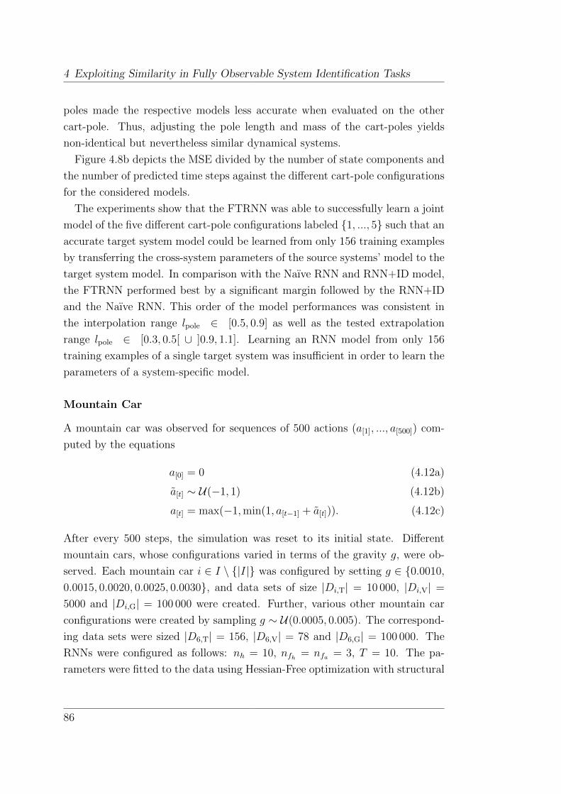
4 Exploiting Similarity in Fully Observable System Identification Tasks
poles made the respective models less accurate when evaluated on the other
cart-pole. Thus, adjusting the pole length and mass of the cart-poles yields
non-identical but nevertheless similar dynamical systems.
Figure 4.8b depicts the MSE divided by the number of state components and
the number of predicted time steps against the different cart-pole configurations
for the considered models.
The experiments show that the FTRNN was able to successfully learn a joint
model of the five different cart-pole configurations labeled 1, ..., 5 such that an
accurate target system model could be learned from only 156 training examples
by transferring the cross-system parameters of the source systems’ model to the
target system model. In comparison with the Naıve RNN and RNN+ID model,
the FTRNN performed best by a significant margin followed by the RNN+ID
and the Naıve RNN. This order of the model performances was consistent in
the interpolation range lpole ∈ [0.5, 0.9] as well as the tested extrapolation
range lpole ∈ [0.3, 0.5[ ∪ ]0.9, 1.1]. Learning an RNN model from only 156
training examples of a single target system was insufficient in order to learn the
parameters of a system-specific model.
Mountain Car
A mountain car was observed for sequences of 500 actions (a[1], ..., a[500]) com-
puted by the equations
a[0] = 0 (4.12a)
a[t] ∼ U(−1, 1) (4.12b)
a[t] = max(−1,min(1, a[t−1] + a[t])). (4.12c)
After every 500 steps, the simulation was reset to its initial state. Different
mountain cars, whose configurations varied in terms of the gravity g, were ob-
served. Each mountain car i ∈ I \ |I| was configured by setting g ∈ 0.0010,
0.0015, 0.0020, 0.0025, 0.0030, and data sets of size |Di,T| = 10 000, |Di,V| =
5000 and |Di,G| = 100 000 were created. Further, various other mountain car
configurations were created by sampling g ∼ U(0.0005, 0.005). The correspond-
ing data sets were sized |D6,T| = 156, |D6,V| = 78 and |D6,G| = 100 000. The
RNNs were configured as follows: nh = 10, nfh = nfa = 3, T = 10. The pa-
rameters were fitted to the data using Hessian-Free optimization with structural
86

4.6 The Fully Observable Transfer Learning Problem
damping (see Section 2.4.2 for details) with the structural damping coefficient
µsd = 0.1 and the initial Levenberg-Marquardt coefficient λLM = 1.0. The
gradient of the optimization objective with respect to the parameters was com-
puted using 10 000 examples selected at random without replacement from the
training data set. During the conjugate gradient (CG) iterations, 5000 exam-
ples from the training data set were selected at random without replacement.
The CG method ran for at most 50 iterations per update. Further, at most
10 000 parameter updates were allowed. These hyperparameters were not ex-
haustively cross-validated, but they were found to work well based on testing
several different settings.
Figure 4.9 depicts the results of the experiments conducted using the moun-
tain car simulation.
Figure 4.9a shows the similarity of all pairs of the five mountain cars labeled
1, ..., 5 by evaluating every RNN model on every mountain car configuration.
Similar to the cart-pole experiments, varying the gravity of the the mountain car
simulation yielded non-identical but similar dynamical systems since a model
trained on a particular mountain car configuration was a less accurate model
of another configuration. The accuracy decreased as the difference of the two
gravity settings increased.
Figure 4.9b depicts the performance of our considered models plotting the
MSE divided by the number of state components and the number of predicted
time steps against the different mountain car configurations.
The mountain car experiments support the results of the cart-pole experi-
ments. Again, the FTRNN performed best by a significant margin followed
by the RNN+ID. The Naıve RNN yielded the largest error among the consid-
ered models. This order of the model performances is consistent in the inter-
polation range g ∈ [0.001, 0.003] as well as the tested extrapolation range
g ∈ [0.0005, 0.001) ∪ (0.003, 0.005]. The error of a simple target system RNN
model using 156 training examples was large and erratic across the set of target
systems. This suggests that it does not suffice to use few training examples of
each target system to learn an accurate model.
87

4 Exploiting Similarity in Fully Observable System Identification Tasks
0 1 2 3 4
Evaluated on mountain car x
0
1
2
3
4
Tra
ined
onm
ounta
inca
ry
10−4
10−3
10−2
10−1
(a) Similarity of the source systems
1 2 3 4 5
·10−3
10−7
10−6
10−5
10−4
10−3
10−2
10−1
100
101
g
1T
dim
(S)ε D
G(h
)
RNN Naıve RNNRNN+ID FTRNN
(b) Error of the target system models
Figure 4.9: Experimental results of the mountain car simulation. The plots
show the mean squared error, evaluated on the generalization data
set sized 100 000, divided by the number of state components and the
number of predicted time steps. (a) compares the similarity of the
source systems by evaluating an RNN model learned from 10 000
training examples of mountain car x and evaluates the model on
mountain car y using the corresponding generalization data set. (b)
compares the error of the different models for various target systems
using 156 training examples to learn the system-specific parameters
of the FTRNN and RNN+ID and all parameters of the RNN. The
dotted vertical lines indicate the source system configurations used
to learn the cross-system parameters of the FTRNN and RNN+ID
as well as the parameters of the Naıve RNN.
88

4.6 The Fully Observable Transfer Learning Problem
4.6.3 Training Time
Besides the ability to exploit prior knowledge in order to decrease the model
error despite only few available observations of a target system, the proposed
transfer learning approach speeded up the training process dramatically. To
demonstrate this additional benefit, the training time of a simple RNN model
given sufficient data was compared with the time it took to train the system-
specific parameters of the FTRNN model given few data. Figure 4.10 visualizes
the training times for the cart-pole and mountain car simulations. As a result,
101 102 103 104 105 106
FTRNN (MC)
RNN (MC)
FTRNN (CP)
RNN (CP)
Training time (seconds)
Figure 4.10: Training times of the RNN and the FTRNN for the cart-pole and
mountain car simulations. The RNN was trained with 10 000 train-
ing examples from a random parameter initialization. In contrast,
the FTRNN was pre-trained on the source systems and only the
system-specific parameters, initialized as the average of the system-
specific parameters of the source systems’ model, were learned from
the training data set of a target system.
the FTRNN was not only able to successfully transfer knowledge from a set of
relevant source systems to an insufficiently observed target system, but it was
also able to achieve high model accuracy within a small fraction of the time
needed to train a comparable RNN model given sufficient training data. The
speed-up for the cart-pole simulation was approximately 25 000× and more than
5000× for the mountain car simulation. Thus, after a joint model of a set of
source systems had been learned, it was possible to adapt the model to a target
system virtually instantaneously.
89
4 Exploiting Similarity in Fully Observable System Identification Tasks
4.6.4 Discussion
The Factored Tensor Recurrent Neural Network (FTRNN) model was presented
which enables efficient knowledge transfer in system identification tasks to learn
the state transition function of a target system from few available observations
given multiple well observed similar source systems. Besides the advantage of
obtaining an accurate model despite few data, learning a target system model
converged within seconds whereas, in contrast, learning an independent model
from scratch, given enough data, often took many hours or even days. In addi-
tion, hyperparameter tuning was significantly reduced despite few data because
the ratio between the amount of training data and the number of adaptive pa-
rameters was reasonable. Last, evaluation of the FTRNN and a standard RNN
have identical complexity because the factored weight matrix per system can be
expanded prior to evaluation.
To demonstrate the effectiveness of the proposed method, experiments were
conducted using the well known cart-pole and mountain car simulations. The
FTRNN model was compared with two more plain approaches to this problem—
the Naıve RNN and the RNN+ID model. The first one was a simple RNN which
learned the state transition function of multiple systems from a concatenated
data set. The second one was a simple RNN with an extra “one-hot” input
vector disclosing the system that generated the example to the model. The
FTRNN performed consistently better than the RNN+ID and the Naıve RNN
using both simulations.
90
CHAPTER 5
Exploiting Similarity in Partially Observable
System Identification Tasks
This chapter addresses the problem of partially observable system identifica-
tion of a target system despite only few available data. Standard modeling
approaches, that learn a model only from the target system data, are inappli-
cable in this setting because the amount of data is insufficient. However, addi-
tional data from related but probably non-identical systems may provide prior
knowledge about the target system and should be utilized in the model building
process. Therefore, several multi-task recurrent neural network architectures,
which are able to utilize information from related tasks as prior knowledge of
the target task, are proposed and empirically evaluated.
The chapter is structured as follows. First, the problem of partially observ-
able system identification in the context of soft-sensor modeling is introduced
and formalized (Section 5.1). Second, a recurrent neural networks architecture
suitable for partially observable system identification is presented (Section 4.2).
Third, the original problem is extended to a multi-system identification task
where only few observations are available from the target system while sufficient
information from auxiliary systems can be utilized (Section 5.3). The recurrent
neural network architectures developed in Section 3.3 are adapted to the par-
tially observable multi-system identification problem. A real-world experiment,
whose goal is to model NOx emissions of Siemens gas turbines, is conducted
employing the multi-task learning paradigm to transfer information from the
auxiliary systems to the target system (Section 5.4). Therefore, multiple vari-
ants of recurrent neural networks are proposed and empirically evaluated.
The subsequent sections are based on the following publication as part of the
doctoral research:
91

5 Exploiting Similarity in Partially Observable System Identification Tasks
• Spieckermann, S., Udluft, S., and Runkler, T. Data-efficient temporal re-
gression with multi-task recurrent neural networks. In Advances in Neural
Information Processing Systems (NIPS), Second Workshop on Transfer
and Multi-Task Learning: Theory meets Practice, 2014.
5.1 Partially Observable System Identification
5.1.1 Introduction
Partially observable system identification is the process of obtaining a model
of a dynamical system using experimental data where the state of the system
cannot be fully observed by the available measuring devices, e.g. sensors. By ag-
gregating a sequence of observations, it may be possible to estimate the state of
the system. Most real-world systems are partially observable. Consider a com-
plex technical system such as a gas turbine equipped with sensors which record
various measurements within the system, e.g. the temperature and pressure af-
ter the compressor before the combustion chamber. Despite the great number
of installed sensors the state of the turbine is not fully observed at a single mo-
ment in time. To overcome partial observability, the observable quantities are
aggregated over time such that the state of the system can be approximated.
5.1.2 Formal Problem Definition
A system, observed in fixed time intervals τ , is defined by the tuple (S,A, f) with
a state space S, an action space A, and an unknown state transition function
f : S × A → S describing the temporal evolution of the state. Further, let
S ′ ⊂ S be a subspace of the state space and gS : S → S ′ be an observation
function which maps S to S ′. Similarly, let gA : A → A′ define an observation
function that maps the action space to a subspace. It is assumed that only S ′
and A′ can be observed.
Let D be a set of observations (x[t−d+1], ..., x[t], y[t]) ∈ D with x[·] ∈ X ⊂S ′ × A′, y[·] ∈ Y , Y ⊂ S ′, X ∩ Y = ∅. Further, let D denote a data set of size
|D| drawn from a probability distribution D.
Let H ⊆ h |h : Xd → Y , d ∈ N, denote a hypothesis space, i.e. a set of
functions that are assumed to approximate the mapping from a sequence of
92

5.2 Partially Observable System Identification with RNNs
state and action observations to a disjoint target state observation. Further,
let L : Y × Y → R denote an error measure between a predicted target y and
the ground truth y. The optimal hypothesis h∗ minimizes the expected error
ε(h) := E(x[t−d+1],...,x[t],y[t])∼D[L(h(x[t−d+1], ..., x[t], y[t])] where E denotes the ex-
pectation operator, hence, h∗ = arg minh∈H ε(h). Since D is generally unknown,
an approximately optimal hypothesis is determined by minimizing the empiri-
cal error εD(h) := 1|D|∑
(x[t−d+1],...,x[t],y[t])∈D L(h(x[t−d+1], ..., x[t], y[t]) induced by a
hypothesis h on a data set D, hence, h = arg minh∈H εD(h).
5.2 Partially Observable System Identification
with Recurrent Neural Networks
Partially observable sequences are often modeled using hidden Markov models
(see Section 2.5). Given a sequence of observations (x[1], ..., x[T ]) the hidden
state transition probabilities and emission parameters are learned such that the
probability of an observed sequence given a corresponding hidden state sequence
is maximized. Thus, learning the parameters of a hidden Markov model may
be considered an unsupervised learning problem. However, the problem class
investigated in this chapter differs from unsupervised sequence learning. Instead
of learning a model of probable sequences, the relationship between a target
variable and a sequence of disjoint environmental and control observations shall
be learned. The model may be viewed as a composite model consisting of a state
estimation sub-model, which infers a hidden state from the sequence of input
observations, and a regression sub-model, which learns the mapping from the
hidden state to the target variable. While it may be possible to stack a hidden
Markov model for the state estimation and, e.g., a linear regression model, this
approach appears unnatural and inefficient since the state estimation is likely
to include information that is irrelevant to the regression task. In contrast,
a model that learns the input-output mapping directly likely aggregates only
relevant information from the input sequence in order to optimally predict the
target variable.
Recurrent neural networks are an appropriate choice to perform state esti-
mation (Schafer & Udluft, 2005; Yadaiah & Sowmya, 2006) with a supervised
target. In order to model a state component of a partially observable dynamical
93

5 Exploiting Similarity in Partially Observable System Identification Tasks
system as a function of other observed state and action variables, a recurrent
neural network may be defined which processes a sequence of state and ac-
tion observations (x[t−d+1], ..., x[t]) yielding the predicted target state variable
y[t]. Instead of predicting only a single step, a technique called overshooting,
i.e. predicting multiple steps, has shown improved results (Zimmermann & Ne-
uneier, 2001; Zimmermann et al., 2007). The network is defined by the following
equations.
h[−d] = 0 (5.1a)
h[t] = φh(Whhh[t−1] +Whxx[t] + bh) (5.1b)
∀t ≥ 1: y[t] = φy(Wyhh[t] + by) (5.1c)
The sequence of state and action observations is mapped to the correspond-
ing hidden state sequence by a linear transformation followed by the nonlinear
function φh(·) which is typically chosen as tanh(·). This allows the network to
learn the extraction of relevant information from different time steps which is
necessary to perform the prediction for t ≥ 1. Depending on the distribution
of y[T ]|x[1], ..., x[T ] a matching activation function φy(·) is chosen. Figure 4.1
x[−1] x[0] x[1] x[2]
1 1 1 1
1 1
h[−1] h[0] h[1] h[2]
Whx Whx Whx Whx
Whh Whh Whh
y[1] y[2]
Wyh Wyh
b y b y
b h b h b h b h
Figure 5.1: Recurrent neural network for partially observable system identifica-
tion.
depicts a graphical representation of the RNN architecture.
94
5.3 Partially Observable Multi-System Identification with RNNs
5.3 Partially Observable Multi-System
Identification with Recurrent Neural
Networks
5.3.1 Naıve RNN
The most naıve approach to exploit information from multiple dynamical sys-
tems and share it with another one is to concatenate the data of all systems
and learn a joint model. This way, the model is forced to generalize over the
different properties of the systems. However, since the training examples of the
systems are not distinguished, the model can only learn the average task which
may be vastly suboptimal for rather different systems.
The following subsections discuss two recurrent neural architectures that are
able to distinguish the systems through an integer identifier. In both models,
the hidden state h[t] accumulates relevant information from past time steps into
an aggregated representation that contains information relevant to the given
learning task.
5.3.2 RNN+ID
One way to incorporate information that allows the model to distinguish be-
tween the systems is to tag each training example with an identifier i ∈ I,
which corresponds to the system that generated the data. This tag may be
provided to the model at each time step as an extra input encoded as the i-th
Euclidean standard basis vector ei with dim(ei) = |I|. The equations of the
RNN+ID architecture are obtained by substituting (5.1b) with (5.2).
h[t] = φh(Whhh[t−1] +Whxx[t] +Whiei + bh) (5.2)
Figure 5.2 depicts a graphical representation of the RNN+ID architecture. In
fact, computing Whiei means selecting the i-th column of Whi so the system
identifier introduces a separate hidden layer bias for each system. The cross-
system bias bh and the specific biases accessed through Whiei can be absorbed
into a new system-specific bias ›Whiei = bh+Whiei. Thus, (5.2) can be rewritten
as
h[t] = φh(Whhh[t−1] +Whxx[t] +›Whiei). (5.3)
95
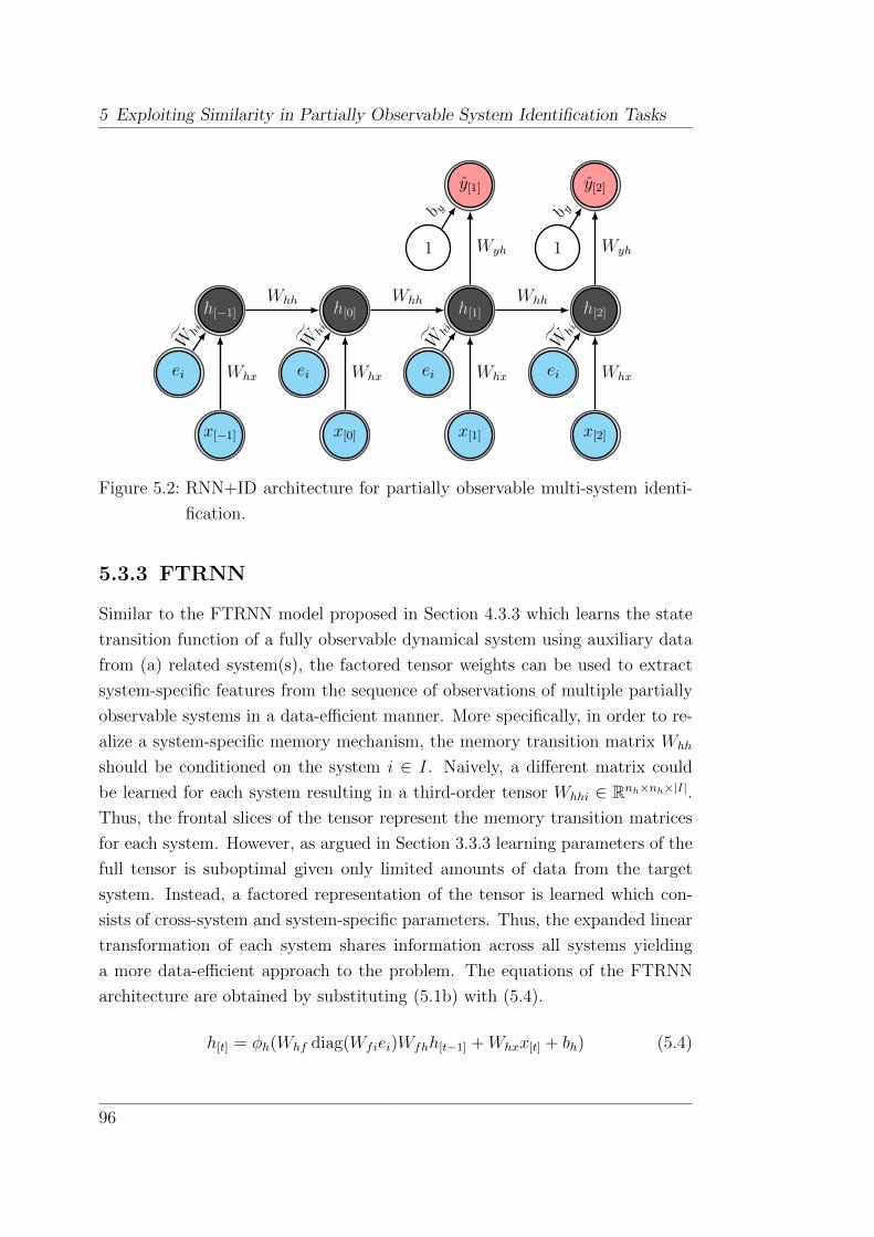
5 Exploiting Similarity in Partially Observable System Identification Tasks
x[−1] x[0] x[1] x[2]
1 1
h[−1] h[0] h[1] h[2]
Whx Whx Whx Whx
Whh Whh Whh
ei ei ei ei
y[1] y[2]W
hi
Whi
Whi
Whi
Wyh Wyh
b y b y
Figure 5.2: RNN+ID architecture for partially observable multi-system identi-
fication.
5.3.3 FTRNN
Similar to the FTRNN model proposed in Section 4.3.3 which learns the state
transition function of a fully observable dynamical system using auxiliary data
from (a) related system(s), the factored tensor weights can be used to extract
system-specific features from the sequence of observations of multiple partially
observable systems in a data-efficient manner. More specifically, in order to re-
alize a system-specific memory mechanism, the memory transition matrix Whh
should be conditioned on the system i ∈ I. Naively, a different matrix could
be learned for each system resulting in a third-order tensor Whhi ∈ Rnh×nh×|I|.
Thus, the frontal slices of the tensor represent the memory transition matrices
for each system. However, as argued in Section 3.3.3 learning parameters of the
full tensor is suboptimal given only limited amounts of data from the target
system. Instead, a factored representation of the tensor is learned which con-
sists of cross-system and system-specific parameters. Thus, the expanded linear
transformation of each system shares information across all systems yielding
a more data-efficient approach to the problem. The equations of the FTRNN
architecture are obtained by substituting (5.1b) with (5.4).
h[t] = φh(Whf diag(Wfiei)Wfhh[t−1] +Whxx[t] + bh) (5.4)
96

5.4 The Partially Observable Multi-Task Learning Problem
Figure 5.3 depicts a graphical representation of the FTRNN architecture.
x[−1] ei x[0] ei x[1] ei x[2]
1 1
1 1 1 1
h[−1] • h[0] • h[1] • h[2]
Whx Whx Whx Whx
Wfh Whf Wfh Whf Wfh Whf
Wfi Wfi Wfi
y[1] y[2]
Wyh Wyh
b y b y
b h b h b h b h
Figure 5.3: FTRNN for partially observable multi-system identification. The
node having the •-symbol in its center is a “multiplication node”,
i.e. the input vectors of the node are multiplied component-wise.
In contrast, the standard nodes imply the summation of all input
vectors.
5.4 The Partially Observable Multi-Task
Learning Problem
The partially observable multi-task learning problem addresses the task of learn-
ing a regression function with temporal dependencies of a little observed par-
tially observable dynamical system by utilizing data from multiple well-observed
similar systems. In order to achieve this goal, the data of all systems are used to
learn a joint model thereof such that information is shared among the systems.
Typical applications of this scenario are situations in which a new instance is
deployed and observed only for a short time until the model, e.g. a soft-sensor,
shall be operational. In case multiple other systems with similar properties, e.g.
systems of the same family, have been operated sufficiently long, the informa-
tion can be utilized as prior knowledge about general structural commonalities
among the systems. Then, the few data from the target system are expected to
suffice in order to learn its peculiarities.
97
5 Exploiting Similarity in Partially Observable System Identification Tasks
5.4.1 Formal Problem Definition
Let I := 1, 2, ... denote a set of identifiers for partially observable deterministic
systems that show similar dynamics. A system, observed in fixed time intervals
τ , is defined by the tuple (S,A, fi), i ∈ I, with a state space S, an action space
A, and an unknown state transition function fi : S × A → S describing the
temporal evolution of the state. Further, let S ′ ⊂ S be a subspace of the state
space and gS : S → S ′ be an observation function which maps S to S ′. Similarly,
let gA : A→ A′ define an observation function that maps the action space to a
subspace. It is assumed that only S ′ and A′ can be observed.
Let Di be a set of observations (i, x[t−d+1], ..., x[t], y[t]) ∈ Di of the i-th system
with x[·] ∈ X ⊂ S ′ × A′, y[·] ∈ Y , Y ⊂ S ′, X ∩ Y = ∅. Further, let D =⋃i∈I Di
denote a data set of size |D| drawn from a probability distribution D.
Let H ⊆ h |h : Xd → Y , d ∈ N, denote a hypothesis space, i.e. a set of func-
tions that are assumed to approximate the mapping from a sequence of state and
action observations to a disjoint target observation. Further, let L : Y ×Y → Rdenote an error measure between a predicted target y and the ground truth y.
The optimal hypothesis h∗i minimizes the conditional expected error εi(h) :=
E(j,x[t−d+1],...,x[t],y[t])∼D[L(h(x[t−d+1], ..., x[t], y[t]) | j = i] where E denotes the expec-
tation operator, hence, h∗i = arg minhi∈H εi(h). Since D is generally unknown,
an approximately optimal hypothesis is determined by minimizing the empir-
ical error εD(h) := 1|D|∑
(·,x[t−d+1],...,x[t],y[t])∈D L(h(x[t−d+1], ..., x[t], y[t]) induced by
a hypothesis h on a data set D, hence, hi = arg minh∈H εDi(h).
Given sufficient data D|I|, it is expected that |ε|I|(h|I|)−ε|I|(h∗|I|)| ≤ ε for some
small positive ε. In contrast, assuming the amount of data D|I| is insufficient,
|ε|I|(h|I|) − ε|I|(h∗|I|)| ε and h|I| may be useless. The problem addressed in
this section is to develop and assess methods that yield a better hypothesis of
an insufficiently observed system through multi-task learning in order to uti-
lize auxiliary information from⋃i∈I\|I|Di as prior knowledge of the transition
function f|I|.
Therefore, the hypothesis space and the empirical error are redefined as fol-
lows. Let H ′ ⊆ h |h : I × Xd → Y denote an extended hypothesis space,
which includes the system identifier into the product space of arguments and
thus jointly approximates the functions of each system. Further, let ε′D(h) :=1|D|∑
(i,x[t−d+1],...,x[t],y[t])∈D wiL(h(i, x[t−d+1], ..., x[t]), y[t]) denote the empirical error
98
5.4 The Partially Observable Multi-Task Learning Problem
of a hypothesis h ∈ H ′ with the system-specific error weight wi. If the the empir-
ically optimal hypothesis h′ = arg minh∈H′ ε′D(h) (D =
⋃i∈I Di) yields a smaller
expected error than h|I|, i.e. ε|I|(h′|I|) < ε|I|(h|I|) with h′i(x[t−d+1], ..., x[t]) :=
h′(i, x[t−d+1], ..., x[t], ), information from the well observed system was success-
fully utilized in the hypothesis search to find a better hypothesis of f|I| despite
few data.
5.4.2 Experiments
The utility of the models presented in Section 5.3 was evaluated on real-world gas
turbine data comprising various hardware configurations. In particular, various
burners had been installed and tested over the course of several weeks during
which sensor data were being collected. The goal was to obtain a model of the
NOx emissions given ambient conditions, e.g. temperature, pressure, humidity,
and control parameters, e.g. angle of the inlet guide vane, position of fuel valves,
in total 23 values per time step. As a result of the different configurations, the
NOx production changed. Despite only relatively few samples of one of the
configurations an accurate NOx model of this instance was required.
Six learning tasks I = 1, ..., 6, each defining the above described modeling
task on data from turbines with different hardware configurations, were avail-
able. Out of the six tasks, five source tasks 1, ..., 5 were selected which served
as prior knowledge for the target task labeled 6. The examples used to train
and evaluate the models were generated by extracting T -step windows of the
sequences of observations. The data sets were decorrelated using the block val-
idation method discussed in Section 2.3.3. The source tasks’ data comprised
6072, 7126, 5448, 8335, and 1361 training examples, and there were 3182 ex-
amples available of the target task 6. In addition, the training examples of
the target task were upsampled to match the average number of samples of the
source tasks. In order to evaluate the model error a test set with 8895 examples
was set aside.
The first step was to gradually gain an understanding of the nature and dif-
ficulty of the task. Therefore, a simple L2-regularized linear regression model,
which learned the mapping X → Y , a multi-step L2-regularized linear regression
Xd → Y mapping a sequence of inputs to the target variable, and a linear RNN
model as described in Section 5.2 with nh ∈ 5, 8, 10, 20 and d = T = 5 were
99

5 Exploiting Similarity in Partially Observable System Identification Tasks
compared. An ensemble of 10 members with randomly initialized parameters
was formed whose predictions were averaged. Figure 5.4 compares the results
of these models using the mean squared error per time step of the zero mean
unit variance NOx targets according to the training set standardization. The
−4,000
−2,000
0
ScaledNO
x
Target Linear Regression
Linear Regression (5 time steps) Linear RNN
0 1,000 2,000 3,000 4,000 5,000 6,000 7,000 8,000 9,000−80−60−40−20
0
Examples of the test set
ScaledNO
x
Figure 5.4: Comparison of the linear model performances in modeling the NOx
emissions of a target gas turbine without knowledge transfer from
other related turbines.
plot shows that none of the linear models was able to accurately predict the
NOx emissions. Among these models, the linear regression which took input
observations from five past subsequent time steps into account, performed best
in relative terms but poorly in absolute terms nevertheless. This result sug-
gested that (i) the linear hypothesis was invalid and (ii) there was a temporal
dependency between the target observation and the inputs, which is expected
in this domain due to delayed effects in the turbine dynamics.
To improve performance, nonlinear RNN models learned only from the tar-
get task data as well as multi-task models, i.e. the Naıve RNN, RNN+ID and
FTRNN, were compared. The models were configured as follows: nfh = nh ∈5, 8, 10, 20, T = 10, d = 5. Ensembles of 10 members with randomly ini-
tialized parameters were formed whose predictions were averaged. Figure 5.5
compares the results of the explored models using the mean squared error per
100
5.4 The Partially Observable Multi-Task Learning Problem
time step of the zero mean unit variance NOx targets according to the train-
ing set standardization. As shown in Figure 5.5a the FTRNN performed best
across the range of considered hidden layer sizes. The RNN+ID yielded a com-
parable but consistently larger error. Compared to the RNN trained only on
the target task data, the two models yielded an improvement on the order of a
factor 10. The Naıve RNN, which was the simplest multi-task learning model
in the comparison, suffered from the auxiliary learning tasks. In order to better
understand the implications of these results the prediction quality of the models
is depicted in Figure 5.5b by comparing their predicted (rescaled) NOx values
with the ground truth. Although the target task RNN outperformed the Naıve
RNN in terms of the MSE it can be observed that it was in fact unable to learn
the input-output relationship but rather predicted a nearly constant value on
the test set. The Naıve RNN appeared to have captured some of the structure of
the input-output relationship, but could not adjust properly to each individual
task. In contrast, the RNN+ID and FTRNN could accurately predict the NOx
emissions despite only few data of the target task.
5.4.3 Discussion
This section demonstrated the utility of multi-task learning in the context of
real-world gas turbine NOx emission modeling. In a first set of experiments gas
turbine NOx emissions were modeled by simple linear models in order to better
understand the difficulty of the task. As it turned out these models were unsuc-
cessful in inferring the relationship between the observable sensor readings and
the NOx emissions from the available data of the target gas turbine. However,
the results indicated that there were temporal dependencies between the NOx
emissions and the input observations likely due to delayed effects in the turbine
dynamics which was a hypothesis consistent with a domain understanding of
the problem at hand. A second set of experiments showed that a recurrent
neural network trained on the target turbine data alone achieved better but
still rather poor predictive performance, too, due to insufficient data. However,
the model was able to predict a small region in the test data comparatively
accurately while the remaining regions appeared to be modeled as an average of
the observed NOx measurements. In order to augment the target turbine data,
auxiliary data from multiple related source turbines were utilized by three vari-
101
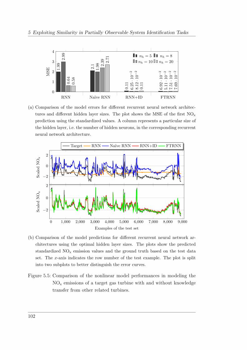
5 Exploiting Similarity in Partially Observable System Identification Tasks
RNN Naıve RNN RNN+ID FTRNN
0
1
2
3
4
1.99
2.1
0.11
6.9
2·1
0−2
2.9
9
1.98
6.25·1
0−2
5.11·1
0−2
0.6
4
2.3
9
8.12·1
0−2
7.51·1
0−2
0.58
2.71
0.1
1
7.69·1
0−2
MS
E
nh = 5 nh = 8
nh = 10 nh = 20
(a) Comparison of the model errors for different recurrent neural network architec-
tures and different hidden layer sizes. The plot shows the MSE of the first NOx
prediction using the standardized values. A column represents a particular size of
the hidden layer, i.e. the number of hidden neurons, in the corresponding recurrent
neural network architecture.
−2
0
2
Sca
led
NO
x
Target RNN Naıve RNN RNN+ID FTRNN
0 1,000 2,000 3,000 4,000 5,000 6,000 7,000 8,000 9,000
−2
0
2
Examples of the test set
Sca
led
NO
x
(b) Comparison of the model predictions for different recurrent neural network ar-
chitectures using the optimal hidden layer sizes. The plots show the predicted
standardized NOx emission values and the ground truth based on the test data
set. The x-axis indicates the row number of the test example. The plot is split
into two subplots to better distinguish the error curves.
Figure 5.5: Comparison of the nonlinear model performances in modeling the
NOx emissions of a target gas turbine with and without knowledge
transfer from other related turbines.
102

5.4 The Partially Observable Multi-Task Learning Problem
ants of recurrent neural network architectures designed to shared information
among all systems. Among them was the novel Factored Tensor Recurrent Neu-
ral Network which encodes cross-system and system-specific information into a
factored third-order tensor. As a result, training a simple RNN (i.e. the Naıve
RNN) on the concatenated source and target system data turned out unsuc-
cessful. The RNN+ID, which received a one-hot encoded task identifier as an
additional input, yielded a significantly more accurate NOx model and, thus,
a significant improvement over simpler approaches. The FTRNN consistently
outperformed all other models.
Multi-task learning is a promising learning paradigm to obtain an accurate
model of a NOx sensor when only few data of a particular target task are avail-
able. Prior knowledge about the relationship between environmental sensor
values and NOx emissions could be incorporated successfully by means of the
Factored Tensor Recurrent Neural Network in the conducted experiments. The
improvement from a model learned only on the target task data to a multi-task
model was significant.
103

5 Exploiting Similarity in Partially Observable System Identification Tasks
104

CHAPTER 6
Conclusions & Future Work
6.1 Conclusions
In this thesis, the problem of data-driven fully and partially observable sys-
tem identification given only few target system data was introduced, motivated
by real-world industrial use cases, and formally defined. Different approaches
to obtain an accurate model of the little observed task of interest were devel-
oped and benchmarked. Knowledge transfer among similar dynamical systems
was explored under three learning paradigms: dual-task learning, multi-task
learning, and transfer learning. In particular, a novel recurrent neural network
architecture—the Factored Tensor Recurrent Neural Network—was proposed.
This network architecture utilizes prior knowledge from similar systems by en-
coding system-specific and cross-system information within a joint model using
factored third-order tensors according to the Parallel Factor Analysis factor-
ization scheme. Therein, system-specific information is encoded in the frontal
diagonal slices of the third-order core tensor. Thus, only few parameters per
system need to be learned compared to the number of cross-system parameters
which are encoded into two full matrices. Therefore, training the model is highly
data-efficient with respect to learning the peculiarities of each individual system.
The architecture is theoretically motivated and inspired by a mathematically
similar formulation previously used in a natural language modeling context. In
addition, a novel regularization technique was proposed for the Factored Tensor
Recurrent Neural Network when used in the dual-task learning setting where
plenty of data from a source system and only few data from a target system
are available. The regularization penalizes diverging system-specific parameters
asymmetrically by tying the parameters of the target system to those of the
105
6 Conclusions & Future Work
source system but not vice versa. Thus, only the target system parameters are
encouraged to remain close to the reliably learned source system parameters,
but biased and/or unreliable information from the target system does not affect
the parameters of the source system sub-model. Experiments were conducted
on two synthetic simulations and real-world gas turbine data.
In all experiments, a naıve model of the respective target task, which was
merely learned from few examples of that task, was unable to generalize well to
a representative set of unseen examples. Augmenting the training examples of
the target task with auxiliary data from one or multiple related task(s) could
improve the unmodified model in most cases, but the resulting performance
was insufficient nevertheless. This observation is explained by the fact that
additional data, although originating from different but related sources, may
help in principle, but the model was not aware that the examples had not been
generated by the same task. Providing the model with task-discriminating infor-
mation was the key to enabling effective and data-efficient knowledge transfer
among related tasks. The obvious approach, in which a task identifier is en-
coded as a “one-hot” vector and fed to the model at each time step, requires no
particular knowledge concerning the nature of the tasks’ similarities and dissim-
ilarities. However, this knowledge was available in the conducted experiments
and it is likely available, at least in part, in real-world problems. Incorporating
it into the model according to the proposed Factored Tensor Recurrent Neural
Network architecture decreased the model error by more than an order of mag-
nitude in some of the conducted experiments. The Factored Tensor Recurrent
Neural Network consistently achieved lower model errors in all experiments.
Although significantly more empirical evidence would be required to support
a general superiority of the Factored Tensor Recurrent Neural Network across a
broad spectrum of problems and applications, this thesis laid out the foundation
of promising research direction to effectively utilize data from related dynamical
systems as prior knowledge of the system of interest. While the Factored Tensor
Recurrent Neural Network was motivated and developed in the context of system
identification tasks, it is in fact a general model suitable for knowledge transfer
among related sequence learning tasks.
106
6.2 Future Work
6.2 Future Work
An interesting continuation of this work may be found in the reinforcement
learning domain. Reinforcement learning has been successfully applied in real-
world industrial use cases (e.g. Schafer et al., 2007a) which are, at the same
time, likely subject to limited data availability. In model-based reinforcement
learning, models of the state transition and reward functions need to be learned
before an optimal policy can be obtained. These models may be difficult to
learn given only few data from the target system. However, when data from
similar systems is available, it is likely possible to learn a better model using
the methods proposed in this thesis. In particular, it would be interesting to
extend the Recurrent Control Neural Network (Schafer et al., 2007b) by the fac-
tored tensor components to enable parameter transfer among multiple related
systems in the model as well as policy learning phases. Thus, not only the state
transition submodel but also the policy submodel might be able to benefit from
the auxiliary information available from related systems. In model-free rein-
forcement learning, learning models of the state transition and reward functions
is bypassed. For instance, a neural network based approach to this problem is
the Policy Gradient Neural Rewards Regression (Schneegaß et al., 2007) which
may be extended by factored tensor components in order to combine informa-
tion from multiple related systems. Investigations along these lines would be
interesting and relevant both academically and with regard to practical appli-
cation. Finally, it would be interesting to conduct studies of the FTRNN model
in the context of other sequence learning problems in order to assess its ability
as a general approach to RNN-based multi-task and transfer learning through
parameter transfer.
107


Bibliography
Ajakan, H., Germain, P., Larochelle, H., Laviolette, F., and Marchand, M.
Domain-adversarial neural networks. In Advances in Neural Information
Processing Systems (NIPS), Second Workshop on Transfer and Multi-Task
Learning: Theory meets Practice, 2014.
Andersen, A. H. and Rayens, W. S. Structure-seeking multilinear methods for
the analysis of fMRI data. NeuroImage, 22(2):728–739, 2004.
Andersen, C. M. and Bro, R. Practical aspects of PARAFAC modeling of
fluorescence excitation-emission data. Journal of Chemometrics, 17(4):200–
215, 2003.
Appellof, C. J. and Davidson, E. R. Strategies for analyzing data from video
fluorometric monitoring of liquid chromatographic effluents. Analytical Chem-
istry, 53(13):2053–2056, 1981.
Bailer-Jones, C. A. L., MacKay, D. J. C., and Withers, P. J. A recurrent neural
network for modelling dynamical systems. Network: Computation in Neural
Systems, 9(4):531–547, 1998.
Barto, A. G., Sutton, R. S., and Anderson, C. W. Neuronlike adaptive elements
that can solve difficult learning control problems. IEEE Transactions on
Systems, Man and Cybernetics, (5):834–846, 1983.
Bastien, F., Lamblin, P., Pascanu, R., Bergstra, J., Goodfellow, I. J., Bergeron,
A., Bouchard, N., and Bengio, Y. Theano: new features and speed im-
provements. In Advances in Neural Information Processing Systems (NIPS),
Workshop on Deep Learning and Unsupervised Feature Learning, 2012.
109
Bibliography
Bayer, J., Osendorfer, C., Korhammer, D., Chen, N., Urban, S., and van der
Smagt, P. On fast dropout and its applicability to recurrent networks. In Pro-
ceedings of the International Conference on Learning Representations (ICLR),
2014.
Bengio, Y. Deep learning of representations for unsupervised and transfer learn-
ing. Journal of Machine Learning Research (JMLR) – Proceedings Track, 27:
17–36, 2012.
Bengio, Y., Simard, P., and Frasconi, P. Learning long-term dependencies with
gradient descent is difficult. IEEE Transactions on Neural Networks, 5(2):
157–166, 1994.
Bengio, Y., Lamblin, P., Popovici, D., and Larochelle, H. Greedy layer-wise
training of deep networks. Advances in Neural Information Processing Sys-
tems, 19:153, 2007.
Bergstra, J., Breuleux, O., Bastien, F., Lamblin, P., Pascanu, R., Desjardins, G.,
Turian, J., Warde-Farley, D., and Bengio, Y. Theano: a CPU and GPU math
expression compiler. In Proceedings of the Python for Scientific Computing
Conference (SciPy), 2010. Oral Presentation.
Breiman, L. Bagging predictors. Machine learning, 24(2):123–140, 1996.
Carroll, J. D. and Chang, J.-J. Analysis of individual differences in multidimen-
sional scaling via an n-way generalization of “eckart-young” decomposition.
Psychometrika, 35(3):283–319, 1970.
Caruana, R. Multitask learning: A knowledge-based source of inductive bias.
In Proceedings of the 10th International Conference on Machine Learning
(ICML), pp. 41–48, 1993.
Caruana, R. Multitask learning. Machine Learning, 28(1):41–75, 1997.
Cattell, R. B. “parallel proportional profiles” and other principles for determin-
ing the choice of factors by rotation. Psychometrika, 9(4):267–283, 1944.
Cybenko, G. Approximation by superpositions of a sigmoidal function. Mathe-
matics of Control, Signals and Systems, 2(4):303–314, 1989.
110

Bibliography
De Lathauwer, L. and Castaing, J. Tensor-based techniques for the blind sepa-
ration of DS-CDMA signals. IEEE Transactions on Signal Processing, 87(2):
322–336, 2007.
Dull, S., Udluft, S., and Sterzing, V. Solving partially observable reinforcement
learning problems with recurrent neural networks. In Neural Networks: Tricks
of the Trade, pp. 709–733. Springer, 2012.
Elman, J. L. Finding structure in time. Cognitive Science, 14(2):179–211, 1990.
Florian, R. V. Correct equations for the dynamics of the cart-pole system.
Center for Cognitive and Neural Studies (Coneural), Romania, 2007.
Forssell, U. and Lindskog, P. Combining semi-physical and neural network mod-
eling: An example of its usefulness. In Submitted to the 11th IFAC Symposium
on System Identification (SYSID’97) to be held in Fukuoka, Japan, 1997.
Girosi, F., Jones, M., and Poggio, T. Regularization theory and neural networks
architectures. Neural Computation, 7(2):219–269, 1995.
Glorot, X., Bordes, A., and Bengio, Y. Domain adaptation for large-scale sen-
timent classification: A deep learning approach. In Proceedings of the 28th
International Conference on Machine Learning (ICML), pp. 513–520, 2011.
Golub, G. H. and van Loan, C. F. Matrix Computations, volume 1. Johns
Hopkins University Press, 1996.
Harshman, R. A. Foundations of the PARAFAC procedure: Models and condi-
tions for an “explanatory” multi-modal factor analysis. 1970.
Harshman, R. A. and Lundy, M. E. PARAFAC: Parallel factor analysis. Com-
putational Statistics & Data Analysis, 18(1):39–72, 1994.
Haykin, S. Neural Networks: A Comprehensive Foundation. Prentice Hall PTR,
Upper Saddle River, NJ, USA, 2 edition, 1998.
Hinton, G. E. and Salakhutdinov, R. R. Reducing the dimensionality of data
with neural networks. Science, 313(5786):504–507, 2006.
111
Bibliography
Hinton, G. E., Srivastava, N., Krizhevsky, A., Sutskever, I., and Salakhutdi-
nov, R. R. Improving neural networks by preventing co-adaptation of feature
detectors. arXiv preprint arXiv:1207.0580, 2012.
Hitchcock, F. L. The expression of a tensor or a polyadic as a sum of products.
Journal of Mathematics and Physics, 6:164–189, 1927.
Hochreiter, S. Untersuchungen zu dynamischen neuronalen netzen. Master’s
thesis, Technical University of Munich – Department of Informatics, 1991.
Hochreiter, S., Bengio, Y., Frasconi, P., and Schmidhuber, J. Gradient flow in
recurrent nets: The difficulty of learning long-term dependencies. In Kremer
and Kolen (eds.), A Field Guide to Dynamical Recurrent Neural Networks.
IEEE Press, 2001.
Hornik, K. Approximation capabilities of multilayer feedforward networks. Neu-
ral Networks, 4(2):251–257, 1991.
Hornik, K., Stinchcombe, M., and White, H. Multilayer feedforward networks
are universal approximators. Neural networks, 2(5):359–366, 1989.
Irsoy, O. and Cardie, C. Modeling compositionality with multiplicative recurrent
neural networks. In Proceedings of the International Conference on Learning
Representations, 2015. Under review.
Jacobs, R. A., Jordan, M. I., Nowlan, S. J., and Hinton, G. E. Adaptive mixtures
of local experts. Neural Computation, 3(1):79–87, 1991.
Jaeger, H. and Haas, H. Harnessing nonlinearity: Predicting chaotic systems
and saving energy in wireless communication. Science, 304(5667):78–80, 2004.
JaJa, J. Optimal evaluation of pairs of bilinear forms. SIAM Journal on Com-
puting, 8(3):443–462, 1979.
Jordan, M. I. and Jacobs, R. A. Hierarchical mixtures of experts and the EM
algorithm. Neural Computation, 6(2):181–214, 1994.
Kohavi, R. and Provost, F. Glossary of terms. Machine Learning, 30(2-3):
271–274, 1998.
112

Bibliography
Kolda, T. G. and Bader, B. W. Tensor decompositions and applications. SIAM
Review, 51(3):455–500, 2009.
Koren, Y. The bellkor solution to the netflix grand prize. Netflix Prize Docu-
mentation, 2009.
Krose, B. and van der Smagt, P. An Introduction to Neural Networks. University
of Amsterdam, Amsterdam, The Netherlands, 1994.
Kruskal, J. B. Three-way arrays: Rank and uniqueness of trilinear decomposi-
tions, with application to arithmetic complexity and statistics. Linear Algebra
and Its Applications, 18(2):95–138, 1977.
Martens, J. Deep learning via Hessian-Free optimization. In Proceedings of the
27th International Conference on Machine Learning (ICML), pp. 735–742,
2010.
Martens, J. and Sutskever, I. Learning recurrent neural networks with Hessian-
Free optimization. In Proceedings of the 28th International Conference on
Machine Learning (ICML), pp. 1033–1040, 2011.
Martens, J. and Sutskever, I. Training deep and recurrent networks with
Hessian-Free optimization. In Neural Networks: Tricks of the Trade, pp.
479–535. Springer, 2012.
Martınez-Montes, E., Valdes-Sosa, P. A., Miwakeichi, F., Goldman, R. I., and
Cohen, M. S. Concurrent EEG/fMRI analysis by multiway partial least
squares. NeuroImage, 22(3):1023–1034, 2004.
Michie, D. and Chambers, R. A. Boxes: An experiment in adaptive control.
Machine Intelligence, 2(2):137–152, 1968a.
Michie, D. and Chambers, R. A. Boxes as a model of pattern formation. In
Waddington, C. (ed.), Towards a Theoretical Biology, volume 1, pp. 206–215.
Edinburgh: Edinburgh University Press, 1968b.
Mikolov, T., Karafiat, M., Burget, L., Cernocky, J., and Khudanpur, S. Re-
current neural network based language model. In Proceedings of the 11th
Annual Conference of the International Speech Communication Association
(INTERSPEECH), pp. 1045–1048, 2010.
113

Bibliography
Minsky, M. L. and Papert, S. Perceptrons: An Introduction to Computational
Geometry. MIT Press, 2 edition, 1988.
Mitchell, B. C. and Burdick, D. S. Slowly converging PARAFAC sequences:
Swamps and two-factor degeneracies. Journal of Chemometrics, 8(2):155–
168, 1994.
Mitchell, T. M. Machine Learning. McGraw-Hill, Inc., New York, NY, USA, 1
edition, 1997. ISBN 0070428077, 9780070428072.
Mitchell, T. M. The need for biases in learning generalizations. In Shavlik,
J. W. and Dietterich, T. G. (eds.), Readings in Machine Learning, pp. 184–
191. Morgan Kauffman, 1980.
Mocks, J. Topographic components model for event-related potentials and some
biophysical considerations. IEEE Transactions on Biomedical Engineering, 35
(6):482–484, 1988.
Neuneier, R. and Zimmermann, H.-G. How to train neural networks. In Neural
Networks: Tricks of the Trade, This Book is an Outgrowth of a 1996 NIPS
Workshop, pp. 373–423. Springer, 1998.
Nocedal, J. and Wright, S. J. Numerical Optimization. Springer, 2 edition,
2006. ISBN 978-0-387-30303-1.
Pan, S. J. and Yang, Q. A survey on transfer learning. IEEE Transactions on
Knowledge and Data Engineering, 22(10):1345–1359, 2010.
Pearlmutter, B. A. Fast exact multiplication by the hessian. Neural Computa-
tion, 6(1):147–160, 1994.
Piotte, M. and Chabbert, M. The pragmatic theory solution to the netflix grand
prize. Netflix Prize Documentation, 2009.
Rabiner, L. A tutorial on hidden Markov models and selected applications in
speech recognition. Proceedings of the IEEE, 77(2):257–286, 1989.
Rehkugler, H. and Zimmermann, H. G. Neuronale Netze in der Okonomie:
Grundlagen und finanzwirtschaftliche Anwendungen. Verlag Vahlen,
Munchen, 1994.
114
Bibliography
Rosenblatt, F. The perceptron: A probabilistic model for information storage
and organization in the brain. Psychological Review, 65(6):386–408, 1958.
Rumelhart, D. E. Learning representations by back-propagating errors. Nature,
323(9):533–536, 1986.
Rumelhart, D. E., Hinton, G. E., and Williams, R. J. Learning representations
by back-propagating errors. Cognitive Modeling, 1988.
Schafer, A. M. and Udluft, S. Solving partially observable reinforcement learning
problems with recurrent neural networks. In Proceedings of the European Con-
ference on Machine Learning (ECML), Workshop on Reinforcement Learning
in Non-Stationary Environments, pp. 71–81, 2005.
Schafer, A. M. and Zimmermann, H.-G. Recurrent neural networks are univer-
sal approximators. In Proceedings of the 16th International Conference on
Artificial Neural Networks (ICANN), pp. 632–640. Springer, 2006.
Schafer, A. M. and Zimmermann, H.-G. Recurrent neural networks are universal
approximators. International Journal of Neural Systems, 17(4):253–263, 2007.
Schafer, A. M., Schneegaß, D., Sterzing, V., and Udluft, S. A neural rein-
forcement learning approach to gas turbine control. In Proceedings of the
International Joint Conference on Neural Networks (IJCNN), pp. 1691–1696,
2007a.
Schafer, A. M., Udluft, S., and Zimmermann, H.-G. The recurrent control neural
network. In Proceedings of the 15th European Symposium on Artificial Neural
Networks, Computational Intelligence and Machine Learning (ESANN), pp.
319–324, 2007b.
Schneegaß, D., Udluft, S., and Martinetz, T. Improving optimality of neural
rewards regression for data-efficient batch near-optimal policy identification.
In Proceedings of the 17th International Conference on Artificial Neural Net-
works (ICANN), pp. 109–118. Springer, 2007.
Sidiropoulos, N. D. and Budampati, R. S. Khatri-rao space-time codes. IEEE
Transactions on Signal Processing, 50(10):2396–2407, 2002.
115
Bibliography
Sidiropoulos, N. D., Bro, R., and Giannakis, G. B. Parallel factor analysis
in sensor array processing. IEEE Transactions on Signal Processing, 48(8):
2377–2388, 2000a.
Sidiropoulos, N. D., Giannakis, G. B., and Bro, R. Blind PARAFAC receivers
for DS-CDMA systems. IEEE Transactions on Signal Processing, 48(3):810–
823, 2000b.
Siegelmann, H. T. and Sontag, E. D. Turing computability with neural nets.
Applied Mathematics Letters, 4(6):77–80, 1991.
Socher, R. Recursive Deep Learning for Natural Language Processing and Com-
puter Vision. PhD thesis, Stanford University, 2014.
Socher, R., Chen, D., Manning, C. D., and Ng, A. Y. Reasoning with neu-
ral tensor networks for knowledge base completion. In Advances in Neural
Information Processing Systems (NIPS), pp. 926–934, 2013a.
Socher, R., Perelygin, A., Wu, J. Y., Chuang, J., Manning, C. D., Ng, A. Y.,
and Potts, C. Recursive deep models for semantic compositionality over a
sentiment treebank. In Proceedings of the Conference on Empirical Methods
in Natural Language Processing (EMNLP), pp. 1631–1642, 2013b.
Spieckermann, S., Dull, S., Udluft, S., Hentschel, A., and Runkler, T. Exploiting
similarity in system identification tasks with recurrent neural networks. In
Proceedings of the 22nd European Symposium on Artificial Neural Networks,
Computational Intelligence and Machine Learning (ESANN), 2014a.
Spieckermann, S., Dull, S., Udluft, S., and Runkler, T. Multi-system identifi-
cation for efficient knowledge transfer with factored tensor recurrent neural
networks. In Proceedings of the European Conference on Machine Learning
(ECML), Workshop on Generalization and Reuse of Machine Learning Mod-
els over Multiple Contexts, 2014b.
Spieckermann, S., Dull, S., Udluft, S., and Runkler, T. Regularized recurrent
neural networks for data efficient dual-task learning. In Proceedings of the 24th
International Conference on Artificial Neural Networks (ICANN), 2014c.
116

Bibliography
Spieckermann, S., Udluft, S., and Runkler, T. Data-efficient temporal regression
with multi-task recurrent neural networks. In Advances in Neural Information
Processing Systems (NIPS), Second Workshop on Transfer and Multi-Task
Learning: Theory meets Practice, 2014d.
Spieckermann, S., Dull, S., Udluft, S., Hentschel, A., and Runkler, T. Exploiting
similarity in system identification tasks with recurrent neural networks. Neu-
rocomputing, (Special Issue ESANN 2014), 2015. Extended version. Invited
paper.
Srivastava, N., Hinton, G. E., Krizhevsky, A., Sutskever, I., and Salakhutdinov,
R. R. Dropout: A simple way to prevent neural networks from overfitting.
The Journal of Machine Learning Research (JMLR), 15(1):1929–1958, 2014.
Stamp, M. A revealing introduction to hidden Markov models,
2004. http://citeseerx.ist.psu.edu/viewdoc/download?doi=10.1.1.
296.4205&rep=rep1&type=pdf.
Sutskever, I., Martens, J., and Hinton, G. E. Generating text with recurrent
neural networks. In Proceedings of the 28th International Conference on Ma-
chine Learning (ICML), pp. 1017–1024, 2011.
Sutskever, I., Martens, J., Dahl, G., and Hinton, G. On the importance of
initialization and momentum in deep learning. In Proceedings of the 30th
International Conference on Machine Learning (ICML), pp. 1139–1147, 2013.
Sutton, R. S. and Barto, A. G. Reinforcement Learning: An Introduction,
volume 1. Cambridge University Press, Cambridge, MA, USA, 1998.
Taigman, Y., Yang, M., Ranzato, M., and Wolf, L. DeepFace: Closing the
gap to human-level performance in face verification. In IEEE Conference
on Computer Vision and Pattern Recognition (CVPR), pp. 1701–1708. IEEE
Press, 2014.
Taylor, G. W. and Hinton, G. E. Factored conditional restricted Boltzmann
machines for modeling motion style. In Proceedings of the 26th International
Conference on Machine Learning (ICML), pp. 1025–1032, 2009.
117
Bibliography
Taylor, M. E. and Stone, P. Transfer learning for reinforcement learning do-
mains: A survey. Journal of Machine Learning Research (JMLR), 10:1633–
1685, 2009.
Ten Berge, J. M. Kruskal’s polynomial for 2× 2× 2 arrays and a generalization
to 2× n× n arrays. Psychometrika, 56(4):631–636, 1991.
Thrun, S. Is learning the n-th thing any easier than learning the first? Advances
in Neural Information Processing Systems (NIPS), pp. 640–646, 1996.
Torrey, L. and Shavlik, J. Transfer learning. In Olivas, E. S., Guerrero, J. D. M.,
Sober, M. M., Benedito, J. R. M., and Lopez, A. J. S. (eds.), Handbook of Re-
search on Machine Learning Applications and Trends: Algorithms, Methods,
and Techniques, volume 1, pp. 242–264. IGI Global, 2009.
Toscher, A., Jahrer, M., and Bell, R. M. The bigchaos solution to the netflix
grand prize. Netflix Prize Documentation, 2009.
Wolpert, D. H. Stacked generalization. Neural Networks, 5(2):241–259, 1992.
Yadaiah, N. and Sowmya, G. Neural network based state estimation of dynami-
cal systems. In International Joint Conference on Neural Networks (IJCNN),
pp. 1042–1049. IEEE, 2006.
Yao, Y., Rosasco, L., and Caponnetto, A. On early stopping in gradient descent
learning. Constructive Approximation, 26(2):289–315, 2007.
Yu, D., Deng, L., and Seide, F. Large vocabulary speech recognition using deep
tensor neural networks. In Proceedings of the 13th Annual Conference of the
International Speech Communication Association (INTERSPEECH), 2012.
Yu, D., Deng, L., and Seide, F. The deep tensor neural network with applications
to large vocabulary speech recognition. IEEE Transactions on Audio, Speech,
and Language Processing, 21(2):388–396, 2013.
Zimmermann, H.-G. and Neuneier, R. Neural network architectures for the
modeling of dynamical systems. In Kolen, J. F. and Kremer, S. C. (eds.),
A Field Guide to Dynamical Recurrent Networks, pp. 311–350. IEEE Press,
2001.
118

Bibliography
Zimmermann, H.-G., Grothmann, R., Schafer, A. M., and Tietz, C. Model-
ing large dynamical systems with dynamical consistent neural networks. In
Haykin, S., Principe, J. C., Sejnowski, T. J., and Mcwhirter, J. (eds.), New
Directions in Statistical Signal Processing: From Systems to Brains, chapter 8,
pp. 203–241. MIT Press, 2007.
119


