Math. Proc. Camb. Phil. Soc. (1997), 121, 147
Printed in Great Britain
147
Multi-symplectic structures and wave propagation
B THOMAS J. BRIDGES
Department of Mathematical and Computing Sciences, University of Surrey,
Guildford, GU2 5XH
(Received 2 June 1994; revised 3 April 1995)
Abstract
A Hamiltonian structure is presented, which generalizes classical Hamiltonian
structure, by assigning a distinct symplectic operator for each unbounded space
direction and time, of a Hamiltonian evolution equation on one or more space
dimensions. This generalization, called multi-symplectic structures, is shown to be
natural for dispersive wave propagation problems. Application of the abstract
properties of the multi-symplectic structures framework leads to a new variational
principle for space-time periodic states reminiscent of the variational principle for
invariant tori, a geometric reformulation of the concepts of action and action flux, a
rigorous proof of the instability criterion predicted by the Whitham modulation
equations, a new symplectic decomposition of the Noether theory, generalization of
the concept of reversibility to space-time and a proof of Lighthill’s geometric
criterion for instability of periodic waves travelling in one space dimension. The
nonlinear Schro$ dinger equation and the water-wave problem are characterized as
Hamiltonian systems on a multi-symplectic structure for example. Further
ramifications of the generalized symplectic structure of theoretical and practical
interest are also discussed.
1. Introduction
An understanding of the existence, propagation, stability, bifurcation, dynamics,
breakup and other properties of wave motion are of fundamental importance in
physical problems such as oceanic waves, atmospheric dynamics, wave guides,
optics, the nervous system, shear flows, acoustics, gas dynamics and many other
areas. In many cases of wave propagation, particularly the equations governing
ocean waves and atmospheric flow, a conservative model is accurate and when
studying conservative partial differential equations it is natural to appeal to the
powerful geometric methods of Lagrangian and Hamiltonian mechanics.
The Lagrangian formulation and the Hamiltonian formulation for a conservative
system are usually considered to be dually related through the Legendre transform
and, in finite dimensions, when the Legendre transform is non-degenerate, the
duality is exact. However in infinite dimensions, particularly systems governing
wave propagation where one or more spatial directions is infinite, the Lagrange–
Hamiltonian duality is no longer uniquely defined. To clarify this point consider
the following elementary example of a nonlinear Klein–Gordon equation
utt®u
xx¯V«(u) x `2, t" 0 (1±1)
148 T J. B
where V(u) is some smooth nonlinear function of u. The Lagrangian formulation for
(1±1) is well understood; the Lagrangian functional for (1±1) is
,¯& t#
t"
&x#
x"
L(u,ut,u
x) dx dt with L(u,u
t,u
x)¯ "
#u#t®"
#u#xV(u) (1±2)
and the equation (1±1) is formally recovered from the Euler–Lagrange equation:
0¯¦¦t 0
¦L
¦ut
1 ¦¦x 0
¦L
¦ux
1®¦L
¦u¯u
tt®u
xx®V«(u).
The Lagrangian formulation of the equations governing wave propagation prob-
lems forms the basis for the Whitham modulation theory for periodic waves
(Whitham[33, 34, 35]) which we will discuss in more detail shortly.
Formally taking the Legendre transform of the Lagrange density L results in a
Hamiltonian formulation; let v¯ ¦L¦ut¯u
t. Then the system (1±1) has ‘the’
Hamiltonian formulation
001®1
0 1¦¦t 0
u
v1¯ 0δHδu
δHδv1 , (1±3a)
where H(u, v)¯&x#
x"
["#v#"
#u#x®V(u)] dx. (1±3b)
An advantage of the Hamiltonian formulation is that the system is in the form of an
evolution equation in time and therefore one can appeal to results in the literature
for existence and other properties of the initial value problem. Another advantage is
the organising structure provided by the symplectic operator. On the other hand, to
be precise, it is necessary to consider a space of functions, including integration over
x, for which the integral of H is well defined. Therefore such a Hamiltonian
formulation is most useful when the spatial domain is finite or when one is interested
in a wave with a particular spatial variation – for example, a spatially periodic wave
or a class of waves that decays exponentially as xU³¢.
However, to say that (1±3) is the Hamiltonian formulation corresponding to (1±1)
or to say that the Hamiltonian formulation (1±3) is dual to the Lagrangian
formulation (1±2) is not completely correct. In effect the Legendre transform leading
to (1±3) is only a partial Legendre transform. A complete Legendre transform would
also eliminate the x-derivatives in the Lagrangian density L(u,ut,u
x). In other words
let w¯ ¦L¦ux¯u
x; then the transformation of equation (1±1), after the complete
Legendre transform, takes the form
MZtKZ
x¯~S(Z) where Z¯
E
F
v
u
w
G
H
`-Z2$, (1±4)
M¯
E
F
®1
0
0
0
1
0
0
0
0
G
H
, K¯
E
F
0
0
1
0
0
0
0
®1
0
G
H
and S(Z)¯ "#(w#®v#)V(u).
The representation (1±4) organizes neatly each facet of the equation. All time
Multi-symplectic structures and wave propagation 149
derivatives appear in the term MZt, all space derivatives appear in the term KZ
xand
the gradient of S(Z) is defined with respect to an inner product on - which in this
case is 2$.
The system (1±4) is a Hamiltonian formulation of (1±1) on a multi-symplectic
structure, since, instead of a single symplectic form, as in (1±3), there are two
pre-symplectic operators M and K – that is ; skew-symmetric and can be identified
with closed two forms – that define a generalized symplectic structure for the system.
To appreciate the distinction between the classical Hamiltonian formulation (1±3),
with a single symplectic operator, and the Hamiltonian formulation on a multi-
symplectic structure in (1±4) it is useful to reconsider the role of the Legendre
transform. In the first, partial, Legendre transform (a) a new set of variables
(u, v)¯def (u,ut) was introduced, (b) a Hamiltonian functional H(u, v) was generated
and (c) an action density was created. The action density in this case is vutand the
gradient of action (with respect to an inner product that includes integration over t)
results in the left-hand side of (1±3) and hence is responsible for generating the
single symplectic operator in the system.
In addition to new variables the complete Legendre transform contributes a family
of action densities and so a family of symplectic operators and in addition a new
Hamiltonian functional is created which is stripped of any explicit derivatives.
In other words a partial Legendre transform and a complete Legendre transform
will lead to non-trivially different symplectic structures and Hamiltonian systems. It
is the main argument, and central organizing feature, of this paper that the
Hamiltonian formulation on a multi-symplectic structure, of the abstract form (1±4)
and its generalization to higher space dimension, is a natural framework for
analysing, and proving particular properties of, dispersive wave propagation in
conservative systems. One of the main results of setting the equations on a multi-
symplectic structure is a framework leading to a rigorous proof of the instability of
periodic travelling waves that is predicted by the Whitham modulation equations.
The Whitham theory for modulation of periodic travelling waves, which was
developed within a Lagrangian framework (Whitham [33, 34, 35]) is summarized as
follows, using (1±1) as an example. Let θ¯ kx®ωt ; then the organizing centre for the
Whitham theory is the averaged Lagrangian
,¯&#π
!
L(u,®ωuθ, kuθ) dθ. (1±5)
The existence theory of such waves proceeds by studying critical points of (1±5)
resulting in a family of periodic travelling waves (u(θ ;ω, k),ω, k). Modulated
travelling waves are treated by allowing ω and k to be slowly varying functions of x
and t. Defining ω¯®θtand k¯ θ
xleads to the kinematic relation
ktω
x¯ 0. (1±6)
Whitham then defines an action and action flux by
!¯¦,
¦ωand "¯®
¦,
¦k(1±7)
150 T J. B
and introduces the conservation of wave action
¦!
¦t
¦"
¦x¯ 0. (1±8)
Combining (1±6) and (1±8) then leads to the coupled Whitham modulation equations
0!ω
0
!k
1 1 9ω
k:t
0"ω
1
"k
0 1 9ω
k:x
¯ 0. (1±9a)
The principal use of the above modulation equations is for predicting the linear
instability of periodic travelling waves of arbitrary amplitude. The linear stability
problem is formulated by taking
0ωk1¯ 0ω!
k!
10ωWkW 1 ei(αx−λt),
where (ω!, k
!) represents the basic periodic state. Linearizing (1±9a) about (ω
!, k
!)
results in the eigenvalue problem
det 9®iλ 0!ω
0
!k
1 1iα 0"ω
1
"k
0 1:¯ 0
and the expression
λ¯α
!ω
["#(!
k®"ω)³o®∆,] !ω 1 0 (1±9b)
for the linear stability exponent, where
∆, ¯®"%(!
k®"ω)#®!ω "
k. (1±10a)
In other words if there exists a root λ `# with )(λ)1 0, equivalently ∆, " 0, there is
an exponentially growing solution of the system (1±9a) linearized about a periodic
travelling wave and hence predicts linear instability. Lighthill [21, 22] noted that
∆, ¯det 0,ωω
,kω
,ωk
,kk
1 (1±10b)
and the following geometric interpretation: if , (or ®,) in (1±5) is a convex function
of ω and k then the basic periodic wave is linearly unstable.
A proof of validity of the Whitham modulation equations would require showing
that solutions of the modulation equation remain near solutions of the original
equations, with respect to a suitably defined norm, on a sufficiently long time scale.
Formal results on the validity have been given by Luke and Whitham using the
method of multiple scales (cf. Whitham[35, §14.4]).
On the other hand the most significant application of the Whitham modulation
equations is to the prediction of linear instability of periodic travelling waves of
arbitrary amplitude. In this paper we formulate rigorously and give a complete proof
of, for periodic travelling waves in one or two space dimensions, the instability result
predicted by the Whitham theory and the geometric instability criterion of Lighthill.
Moreover the reformulation of the problem leads not only to a precise list of the
Multi-symplectic structures and wave propagation 151
hypotheses under which the theory is valid, and a complete proof, but also to further
results including dual geometric criteria for instability. It is precisely the multi-
symplectic structures framework and a geometric reformulation of the concepts of
action and action flux that make a rigorous theory possible.
The concepts of action and action flux and the conservation of wave action are
recognized as fundamental concepts in wave propagation and, since they were
introduced by Whitham, there has been significant generalizations of action and its
relatives (Hayes[18, 19], Andrews & McIntyre[1], Grimshaw[17] and references
therein). However in the definition of action and action flux in (1±7), and all related
definitions in the literature, the action and action flux are defined in terms of
averaged quantities. The lack of structure in the definition of action and action flux
is an obstacle to a rigorous theory. One of the main results of this paper is to define
primitive functionals for action and action flux; they are one-forms whose exterior
derivative results in closed two forms and it is precisely the structure of the closed
two forms that forms a basis for the rigorous theory of wave instability.
Although many of the properties of wave dynamics can be appreciated
within a Lagrangian framework, a Hamiltonian framework is a useful one within
which to prove results. A prototype is the water wave problem. The Lagrangian
formulation for water waves was discovered before the Hamiltonian formulation
and many properties of waves were illuminated in the Lagrangian framework (cf.
Whitham[34, 35]). However the later discovery of a Hamiltonian formulation (cf.
Zakharov[36], Broer[15]) for water waves lead to proofs, and in particular geometric
proofs, of many facets of the water-wave problem. For example Benjamin & Olver[5]
were able to enumerate rigorously, and prove finiteness of, the set of conservation
laws for water waves; Saffman[31] gave a geometric proof of the superharmonic
instability of water waves that used only the Hamiltonian structure and MacKay &
Saffman[23] defined a signature invariant of the eigenspace corresponding to the
linear stability problem for water waves, using the symplectic operator, that proved
useful for classifying instabilities of large-amplitude travelling water waves. However
in the results above on water waves a partial Hamiltonian structure was used; a
classical Hamiltonian structure with a single symplectic operator. By considering the
water wave problem as a Hamiltonian system on a multi-symplectic structure
further results are possible. In Bridges & Mielke[13] a proof of the Benjamin–Feir
instability is given which relies crucially on the interplay between the spatial and
temporal symplectic structures. In Bridges[11] the multi-symplectic structures
framework is applied to formulate the instability problem for arbitrary periodic
patterns, interacting with a mean flow in finite depth, on the ocean surface.
Abstractly, we call the formulation represented by (1±4), and its generalizations, a
Hamiltonian system on a multi-symplectic structure and as far as we are aware the
formulation and analysis of a such a structure is new. A symplectic structure (-,ω)
consists of a manifold -, the phase space, on which there is a non-degenerate closed
two-form. A Hamiltonian system is then a triplet (-,ω,H) where H : -U2 is a
functional. The generalisation of this, a multi-symplectic structure (-,ω("),…,ω(n)),
consists of a manifold -, the phase space, and a family of closed, in general non-
commuting, two-forms. In the multi-symplectic case we relax the requirement of
non-degeneracy; a closed but possibly degenerate two-form is usually called pre-
symplectic (cf. Marsden[25, p. 29]) but the distinction is not important in the present
152 T J. B
theory. A Hamiltonian system on a multi-symplectic structure is then represented
symbolically by (-,ω("),…,ω(n),S) with governing equation
ω(") 0¦Z
¦t,61…ω(n) 0 ¦Z
¦xm
,61¯©~S(Z),6ªm
(1±11)
for all 6 `Tm
- where ©[, [ªm
is an inner product on Tm
- at m `-. For
definiteness we will suppose that the system is tri-symplectic (two space dimensions
and time) with
ω(")(Zt,6)¯def©M(Z)Z
t,6ª
m,
ω(#)(Zx,6)¯def©K(Z)Z
x,6ª
m,
ω($)(Zy,6)¯
def
©L(Z)Zy,6ª
m.
When the inner product ©[, [ªm
is independent of m `- the system (1±11) may be
written
M(Z)ZtK(Z)Z
xL(Z)Z
y¯~S(Z) Z `-. (1±12)
In general the phase space - is a manifold modelled on 2n, or in infinite dimensions
a Hilbert or Banach space. To avoid unnecessary technicalities we will take - to be
a linear space unless noted otherwise.
The formulation (1±11)–(1±12) has properties that make it natural for studying
wave propagation in open systems. In fact the components of the formulation (1±11),
the Hamiltonian functional S and the skew-symmetric operators M(Z), K(Z) and
L(Z), can be identified with quantities that are known to be important for wave
propagation in conservative systems. In one space dimension the Hamiltonian
functional S(Z) is related to the flow force, or in some cases the momentum flux, for
the system (see Appendix B). The definition of the flow force and its implications for
wave propagation are discussed in Benjamin[3] and references therein. In two space
dimensions the connection between S(Z) and a physically relevant functional is not
so clear. The operators M(Z), K(Z) and L(Z) are structure operators for the action
and action-flux vector.
The hypothesis of closedness for the symplectic operators M(Z), K(Z) and L(Z) is
necessary to ensure that, at least locally, the terms M(Z)Zt, K(Z)Z
xand L(Z)Z
yare
gradients of certain functionals. In order to avoid unnecessary technicalities we will
also assume that the symplectic operators are associated with two-forms that are
exact, which is often the case in applications, in which case the terms M(Z)Zt,…,
are globally defined as gradient operators. In particular there exist, formally,
functionals A(Z), B"(Z) and B
#(Z) such that
~A¯M(Z)Zt
~B"¯K(Z)Z
x
~B#¯L(Z)Z
y
where the gradients are defined with respect to an inner product that includes
integration over x, y or t. The densities A, B"
and B#
are independent action
functionals for the t, x and y directions respectively and can be identified with one-
Multi-symplectic structures and wave propagation 153
forms; that is, there exist, formally, vector-valued functions α(Z), β"(Z) and β
#(Z)
such thatA(Z)¯©α(Z),Z
tªm
B"(Z)¯©β
"(Z),Z
xªm
B#(Z)¯©β
#(Z),Z
yªm. (1±13)
When the inner product does not depend explicitly on m `- there is a simple
relation between the forms α, β"
and β#
and the symplectic operators, namely
M(Z)¯Dα(Z)*®Dα(Z)
K(Z)¯Dβ"(Z)*®Dβ
"(Z)
L(Z)¯Dβ#(Z)*®Dβ
#(Z) (1±14
where D represents differentiation on the phase space (when - is finite dimensional
it is the Jacobian operation) and n indicates formal adjoint. For example for the
multi-symplectic structure presented in equation (1±4) for the wave equation (1±1) the
action one-forms are
A(Z)¯©α(Z),Ztª with α(Z)¯
E
F
0
v
0
G
H
,
B(Z)¯©β(Z),Zxª with β(Z)¯
E
F
0
w
0
G
H
,
where, here, ©[, [ª is the standard inner product on 2$. In this case the Jacobian
operation is the usual derivative and the adjoint operation is matrix transposition.
When ensemble averaged or averaged over a phase, the values of the functionals
!, ""
and "#, which represent the averaged values of A, B
"and B
#, recover the
Whitham–Hayes definition of action and (two-component) action flux respectively.
Although, in the present formulation, a conservation law for action is neither implied
nor required but for historical reasons we refer to the primitive definitions in (1±13),
even without averaging, as the action and action-flux densities.
A remarkable consequence of the formulation (1±11)–(1±12) is that a number of
general results about waves can be derived and in some cases rigorously proved using
only the abstract properties of the mult-symplectic structure. In Section 2 a new
variational principle for space and time periodic states is introduced. In one-space
dimension the idea can be seen using (1±12) restricted to one space dimension. With
τ¯ωt and ξ¯ kx (1±12), restricted to one space dimension and 2π-periodic, in (ξ, τ),
functions is transformed to
ωM(Z)¦Z
¦τkK(Z)
¦Z
¦ξ¯~S(Z) with (τ, ξ) `4#. (1±15)
However since M(Z)Zτ and K(Z)Zξ are gradients of functionals A and B"respectively
(averaged over 4#) the equation (1±15) is formally the Lagrange necessary condition
for the constrained variational principle
crit (3) r!=I",""=I#
(1±16)
154 T J. B
in which case ω and k are Lagrange multipliers. The generalization of this variational
principle to two-space dimensions is
crit (3) r!=I",""=I#,
"#=I$
(1±17)
with ω, k and l as Lagrange multipliers, where l is the wavenumber in the y-direction.
The variational principles given by (1±15)–(1±17) are analogous to the variational
principles for invariant toroids of finite-dimensional Hamiltonian systems (cf.
Percival[30]).
It is an elementary consequence of the Lagrange multiplier theory (cf. Section 2)
that
ω¯¦S
¦I"
, k¯¦S
¦I#
, and l¯¦S
¦I$
;
that is, the frequency and wavenumbers are given by certain slopes in S versus action
space. The above identities also lead to
HessI(3)¯
E
F
S#"
S##
S#$
S""
S"#
S"$
S$"
S$#
S$$
G
H
¯
E
F
¦k
¦I"
¦ω
¦I"
¦l
¦I"
¦k
¦I#
¦ω
¦I#
¦l
¦I#
¦k
¦I$
¦ω
¦I$
¦l
¦I$
G
H
(1±18)
where Sij¯ ¦#S¦I
i¦I
jfor i, j¯ 1, 2, 3. It is shown in Section 2 that a necessary
condition for the variational principle for waves to be non-degenerate is that
∆S¯defdet (Hess
I(3))1 0.
It is interesting that this non-degeneracy condition is reminiscent of the non-
degeneracy condition for invariant tori in the KAM theory (cf. Percival[30]).
In Section 3 the properties of the Whitham modulation equations for periodic
travelling waves in two space dimensions are recalled and they are cast into a form for
comparison with the variational principle of Section 2 and the rigorous theory of
Section 4. The important point here is to indicate precisely what one can prove using
the methods of this paper about the Whitham modulation equations. In particular
a proof is given of the validity of the linear instability results predicted by the
Whitham theory. By checking the hypotheses of Theorem 4±1 in Section 4 it is clear
also that a wave state predicted by the Whitham modulation equations to be stable
is not necessarily stable in the full system from which the equations were derived.
In Section 4 a rigorous theory for the instability of periodic waves of arbitrary
amplitude travelling in two space dimensions is presented. In the stability analysis the
existence of a basic state is taken as a hypothesis and it is of the form
²ZW (θ ; I), ω(I), k(I), l(I) ; θ¯ kxly®ωt, I `5Z2$´ (1±19)
and satisfies (1±12). The dependence on the parameters I", I
#and I
$(level sets of the
action constraint sets) is assured by the variational principle of Section 2. The main
result of Section 4 is a proof of the relation between the stability exponent of the
system (1±12) linearised about the basic state (1±19) and the fundamental matrix
Multi-symplectic structures and wave propagation 155
HessI(3) of the basic state. The result of Theorem 4±1 is precisely a proof of the
instability result predicted by the Whitham modulation equation. The proof however
does not appeal to the conservation of wave action nor the Whitham modulation
equations but works directly with the governing equations appealing instead to the
geometry presented by the multi-sympletic structures framework. Theorem 4±1 also
connects explicitly the linear stability exponents and the fundamental matrix
HessI(3) in (1±18). In terms of Hess
I(3) the instability result is
E if HessI(3) is positive definite the wave is linearly unstable;
E if S##
S$$
®S#$
S$#
! 0 the wave is linearly unstable;
E if S##
S$$
®S#$
S$#
" 0 but S$$
∆K
" 0 the wave is linearly unstable.
The proof of instability for waves travelling in one space dimension follows similar
lines – indeed is a special case – but has some interesting features that are treated
separately in Section 5. In particular a proof of Lighthill’s geometric criterion is
given and moreover the proof is obtained by first showing that there is a dual
criterion for instability in terms of the geometry of the flow force on action space.
In Section 6 two examples are treated, the Nonlinear Schro$ dinger (NLS) equation
and the water-wave problem on an infinite-depth fluid both for the case of two space
dimensions. The purpose of Section 6 is to illustrate how the theory of the present
paper applies to wave instability problems that are generally well understood. For
the NLS equation the hypotheses of Theorem 4±1 in Section 4 can be explicitly
verified and application of the theory to NLS leads to interesting geometric
properties of the instability. For the water-wave problem the application of the
theory in Section 6 is formal ; this example is a precursor to more complete results
that we presented elsewhere. A complete proof of instability for water waves
travelling in one space dimension has been given in Bridges & Mielke[13]. Also in a
companion paper (Bridges[11]) complete details of the application of the present
theory to the instability problem for periodic patterns on the ocean surface affected
by mean-flow dynamics is given.
Some auxiliary results are presented in the Appendices. A fundamental concept in
the theory of classical Hamiltonian systems is the interplay between reversibility and
symplecticity. The generalization to the multi-symplectic framework is presented in
Appendix A.
An advantage of the multi-symplectic structures framework is that it decomposes
neatly the different facets of the governing equation. Appendix B shows how the
impulse and action are simply related in the framework leading to a useful
decomposition of the impulse and energy conservation laws.
When a conservative system has a Hamiltonian structure the symplectic operator
gives a natural correspondence between symmetries and invariants (Olver[28, 29]).
But the classical theory does not establish a relation between symplecticity and
fluxes. Such a connection is only possible by introducing additional sympletic
operators. In Appendix C a new decomposition of the Noether theory is given using
the multi-sympletic structures theory. Such a decomposition is of fundamental
importance when analysing the stability of waves in the presence of symmetry or
mean-flow effects (cf. Bridges[11]). Finally, in Appendix D some special properties
of the Hamiltonian functional on a multi-symplectic structure are presented.
156 T J. B
2. Toral geometry and variational principles for space-time periodic states
The restriction of the generalized Hamiltonian structure (1±11) or (1±12) to 4n ; that
is, functions that are periodic in n-directions leads to a new constrained variational
principle for space and time periodic waves. Here we consider the wave states that
are periodic in 2-space dimensions and time.
Scale x, y and t so that the system (1±12) is restricted to 2π-periodic functions
τ¯ωt, ξ¯ kx, ζ¯ ly with (ξ, ζ, τ) `4$.
Then (1±12) becomes
ωM(Z)ZτkK(Z)ZξlL(Z)Zζ ¯~S(Z) with Z : 4$U-. (2±1)
Because of the hypothesis that M(Z), K(Z) and L(Z) are associated with closed two
forms, the terms M(Z)Zτ, K(Z)Zξ and L(Z)Zζ can be identified with the gradients of
certain functionals,~A(Z)¯M(Z)Zτ
~B"(Z)¯K(Z)Zξ
~B#(Z)¯L(Z)Zζ,
where here the gradient is defined with respect to an inner product that includes
integration over 4$. Therefore (2±1) can be written
~S(Z)¯ω~A(Z)k~B"(Z)l~B
#(Z) (2±2)
which can equivalently be characterized in terms of a constrained variational
principle.
Variational principle for space-time periodic states. Space-time periodic states of
the Hamiltonian system (1±12) on the multi-symplectic structure (-,ω(")m
,ω(#)m
,ω($)m
,S)
correspond to the critical points : ZW : 4$U- of S restricted to level sets of the action
functionals !, ""
and "#
or
crit ²S : !¯ I", "
"¯ I
#and "
#¯ I
$´, (2±3)
where I `5Z2$ are values of the action level sets.
The symbols 3, !, ""and "
#correspond to S, A, B
"and B
#, respectively, averaged
over 4$. The verification of the above variational principle follows from the Lagrange
multiplier theory. The statement is formal ; application to particular examples
may encounter technical difficulties such as small divisors. On the other hand it
leads to interesting structural properties of the solutions including linear stability
information (cf. Section 4).
An interesting property of the above variational principle is its relation with the
variational principle for invariant toroids of finite-dimensional Hamiltonian systems.
This correspondence has been discussed in Bridges[9] for plane waves on one-space
dimension in the context of the nonlinear Schro$ dinger equation. However, the
connection with invariant tori is more general and follows from the multi-symplectic
structure.
For example, consider the finite-dimensional Hamiltonian system
JUt¯~H(U) with U `-Z2' (2±4)
Multi-symplectic structures and wave propagation 157
and J the standard symplectic operator on 2'. Restrict (2±4) to an invariant torus by
taking coordinates ξ¯ (ξ", ξ
#, ξ
$) `4$ with ξ
j¯ω
jt for j¯ 1, 2, 3. Then (2±4) restricted
to 4$ becomes
ω"J¦U
¦ξ"
ω#J¦U
¦ξ#
ω$J¦U
¦ξ$
¯~H(U). (2±5)
The most significant difference between (2±1) and (2±5) is the symplectic operators. In
(2±5) the symplectic operators commute, indeed are the same, whereas in (2±1) the
symplectic operators are different and in general non-commutative. Introduce
actions for the tori satisfying (2±5),
Ij¯,
4$
"#©U, J¦ξ
j
Uª2'dξ j¯ 1, 2, 3.
It is evident that, formally, (2±5) is the Lagrange necessary condition for the
variational principle of finding critical points of the Hamiltonian on level sets of the
actions with ωj, j¯ 1, 2, 3, treated as Lagrange multipliers ; this is in fact Percival’s
first variational principle for invariant tori of fixed action (cf. Percival[30]). The
relation of the variational principle (2±3) with invariant toroids is further emphasized
below where it is shown that the variational principle (2±3) is non-degenerate if the
frequency map is non-degenerate which is reminiscent of the non-degeneracy
condition for invariant toroids of finite-dimensional Hamiltonian systems.
The Lagrange necessary condition for the variational principle (2±3) is that Z `-
should satisfy
~&¯ 0 with &(Z ;ω, k, l)¯3(Z)®ω!(Z)®k""(Z)®l"
#(Z) (2±6)
as well as the three constraints. A basic solution of the variational principle depends
on I `2$ in the following way
²ZW (ξ, ζ, τ ; I), ω(I), k(I), l(I) ; I¯ (I", I
#, I
$) `5Z2$´. (2±7)
This is verified as follows. A solution of (2±6) has the form Z(ξ, ζ, τ ;ω, k, l) ; but
substitution of this expression into the constraint set results in
!(Z(ξ, ζ, τ ;ω, k, l))¯ I"
""(Z(ξ, ζ, τ ;ω, k, l))¯ I
#
"#(Z(ξ, ζ, τ ;ω, k, l))¯ I
$
5
6
7
8
(2±8)
which when inverted leads to ω(I), k(I) and l(I). Back substitution into
Z(ξ, ζ, τ ;ω, k, l) leads to the dependence in (2±7). Note however that (2±8) is solvable,
by an implicit function theorem argument, if and only if det (D)1 0 where
D¯
E
F
¦k
¦I"
¦ω
¦I"
¦l
¦I"
¦k
¦I#
¦ω
¦I#
¦l
¦I#
¦k
¦I$
¦ω
¦I$
¦l
¦I$
G
H
. (2±9)
In the analysis of Section 4 it will be shown that the matrix (2±9) contains linear
stability information. It is also reminiscent of the frequeny map on action space in
the KAM theory. The variational principle (2±3) is non-degenerate if det (D)1 0. The

158 T J. B
matrix D is symmetric. The symmetry of D can be seen by using the following
identities
ω(I)¯¦3
¦I"
, k(I)¯¦3
¦I#
and l(I)¯¦3
¦I$
. (2±10)
These identities follow from the classical Lagrange multiplier theory and are verified
as follows: for j¯ 1, 2, 3 we have that
¦3
¦Ij
¯ 9~S(Z),¦Z
¦Ij
:¯ 9ω~A(Z)k~B
"(Z)l~B
#(Z),
¦Z
¦Ij
:¯ω
¦!
¦Ij
k¦"
"
¦Ij
l¦"
#
¦Ij
¯ωδ"jkδ
#jlδ
$j.
Using the identities (2±10) it follows that the matrix D can also be represented as
D¯HessI(3)¯
E
F
S#"
S##
S#$
S""
S"#
S"$
S$"
S$#
S$$
G
H
where Sij
¯def¦#3
¦Ii¦I
j
. (2±11)
A sensitivity matrix of the form (2±9) carries information about critical point type
for constrained variational principles with a well-defined Morse index (cf.
Maddocks[24]). However critical point type for solutions of the variational principle
(2±3) is not well-defined. The second variation of & in (2±6) defined by
,¯D#&(Z ;ω, k, l)¯D#S(Z)®ωD#A(Z)®kD#B"(Z)®lD#B
#(Z)
has a countable number of negative as well as positive eigenvalues. This can be easily
seen already in the case when space variation is absent (i.e. &¯3(Z)®ω!(Z))
which is just Hamilton’s principle for periodic orbits of classical Hamiltonian
systems. Technically the critical points are saddle points of infinite order. However
we will be able to extract useful information about linear stability from the
constrained variational principle and sensitivity matrix by working directly with the
linear stability problem (Section 4).
Finally we remark that the variational principle (2±3) is for nonlinear states. It has
no meaning for the linear problem – it is trivially degenerate. In the linear problem
the frequency and wavenumbers are related by the dispersion relation and therefore
the columns of the matrix D in (2±9) will be linearly dependent resulting in
degeneracy.
3. Structure of Whitham’s modulation equations
The Whitham theory for modulated travelling waves in two space dimensions, in
the absence of mean flow effects, is based on the equations
ky®l
x¯ 0
ktω
x¯ 0
ltω
y¯ 0
(!)t®("
")x®("
#)y¯ 0. (3±1)
Multi-symplectic structures and wave propagation 159
The first three of these are kinematic conditions on the phase θ and
ω¯®θt, k¯ θ
xand l¯ θ
y(3±2)
are interpreted as slowly varying functions of x, y and t. The fourth equation of (3±1)
is the hypothesis of conservation of wave action where !, ""and "
#are averages of
the action and action fluxes respectively that are considered as slowly varying
functions of x, y and t (cf. Whitham[34, 35] and Hayes[18, 19]).
In this section we will first make some observations about the Hamiltonian
structure of the equations (3±1). Then the equations will be cast into a form where the
instability of waves predicted by (3±1) can be compared with the information
generated by the variational principle of Section 2 and the rigorous theory to be
presented in Section 4.
First we remark that the first three equations of (3±1) correspond to a Hamiltonian
system; they can be rewritten in the form
E
F
0
0
0
0
0
®1
1
0
0
G
H
E
F
k
ω
l
G
H
¯
E
F
®ωy
ky®l
x
ωx
G
H
(3±3)
or J"Ω
t¯~H(Ω), where Ω¯
E
F
k
ω
l
G
H
, J"¯
E
F
0
0
0
0
0
®1
1
0
0
G
H
and H(Ω)¯&y#
y"
&x#
x"
ω(ky®l
x) dx dy.
With suitable fixed endpoint conditions for Ω on the boundary of the rectangle
[x", x
#]¬[y
", y
#] the gradient of H(Ω) is
~H(Ω)¯def
E
F
δHδk
δHδω
δHδl
G
H
¯
E
F
®ωy
ky®l
x
ωx
G
H
.
The governing equation for Ω has another interpretation as a Hamiltonian system
on a multi-symplectic structure. First note that
~H(Ω)¯
E
F
®ωy
ky®l
x
ωx
G
H
¯
E
F
0
®lx
ωx
G
H
0 ky
®ωy
1¯®J#Ω
x®J
$Ω
y,
where J#¯
E
F
0
0
®1
0
0
0
0
1
0
G
H
and J$¯
E
F
1
0
0
0
®1
0
0
0
0
G
H
.
Therefore the set (3±1) has the equivalent representation
J"Ω
tJ
#Ω
xJ
$Ω
y
(!)t®("
")x®("
#)y
¯ 0
¯ 0.* (3±4)

160 T J. B
The governing equation for Ω is a Hamiltonian system on a multi-symplectic
structure: (2$,ω("),ω(#),ω($)) with
ω(")¯ dkgdl, ω(#)¯ dωgdl and ω($)¯ dkgdω
with trivial Hamiltonian function. Moreover it is interesting to note that the
symplectic forms ω("), ω(#) and ω($) form a basis for the Lie algebra so(3).
In light of the variational principle of Section 2, a reasonable hypothesis is to
suppose that ω, k and l depend only on the values of the actions !, ""and "
#and
do not otherwise depend explicitly on x, y and t. Therefore define
D¯
E
F
~k
~ω
~l
G
H
where ~ is a gradient on action space. Then
Ωt¯D)
twhere )¯
E
F
""
!
"#
G
H
with similar expressions for Ωx
and Ωy. On action space the coupled equations (3±4)
then become
J"D)
tJ
#D)
xJ
$D)
y
©e",)
tª®©e
#,)
xª®©e
$,)
yª
¯ 0
¯ 0(3±5)
where e", e
#and e
$are unit vectors on 2$ and here ©[, [ª represents the standard inner
product on 2$ (compare with Hayes[19, equations (3±1)–(3±2)]).
Let )!
be some fixed constant value on action space representative of a periodic
travelling wave in two space dimensions and linearize (3±5) about this state with
)¯)!)W ei(αx+βy−λt)
where (α,β) `2# and λ `#. Then the linearization of (3±5) about )!
becomes
[®λJ"αJ
#βJ
$]D)W
©Γ,)W ª¯ 0
¯ 0* (3±6)
where Γ¯λe"αe
eβe
$and D is now evaluated at )
!. Supposing rλr#α#β#1 0,
Kernel [®λJ"αJ
#βJ
$]¯ span ²Γ´.
Therefore the general solution of the first equation of (3±6) is
D)W `Kernel [®λJ"αJ
#βJ
$]3)W ¯ cD−"Γ
for some non-zero scalar c. Substitution into the second equation of (3±6) results in
c©Γ,D−"Γª¯ 0.
Therefore define
Λ#(λ,α,β)¯©Γ,D−"Γª¯
E
F
α
λ
β
G
H
,
E
F
k"
ω"
l"
k#
ω#
l#
k$
ω$
l$
G
H
−"E
F
α
λ
β
G
H
. (3±7)
Multi-symplectic structures and wave propagation 161
The interpretation of (3±7) in terms of (3±5) is as follows. If for some (α,β) `2#, there
exists a λ `# with )(λ)1 0 and Λ(λ,α,β)¯ 0 there exists an unstable solution near
)!
on action space.
This completes the reappraisal of the Whitham modulation equations. In Section
4 we will give a proof of the above instability criterion and the proof is given without
direct recourse to the modulation equations or the conservation of wave action.
4. A rigorous geometric theory for plane wave instability
In this section the linear instability problem for periodic travelling waves of the
systemM(Z)Z
tK(Z)Z
xL(Z)Z
y¯~S(Z), (4±1)
where M(Z), K(Z), L(Z) and S are identified with a multi-symplectic structure and
the skew-symmetric operators are in general Z-dependent, is formulated rigorously.
The basic state is a travelling plane wave of the form ZW (θ, [) with θ¯ kxly®ωt. A
connection is established between the stability exponent in the time-dependent
problem and the ‘KAM matrix’ HessI(S) that arises in the variational principle of
Section 2. The instability criterion is established independent of the particular
equation and relies only on the geometry of the multi-symplectic structure.
Introduce new coordinates
θ¯ kxly®ωt, y«¯ y and t«¯ t ;
in terms of which equation (4±1) becomes
M(Z)Zt«L(Z)Z
y«J(Z)Zθ ¯~S(Z) (4±2)
where, for simplicity the primes on y, t will henceforth be dropped, and
J(Z)¯ kK(Z)lL(Z)®ωM(Z). (4±3)
It is taken as a hypothesis that there exists a basic travelling wave state of the
form
(H1) ²ZW (θ ; I), ω(I), k(I), l(I) ; I `5Z2$´
and that ω, k and l are sufficiently smooth so that the matrix D in (2±9), evaluated
at the basic state, is well defined and non-degenerate and ZW is sufficiently
differentiable. It follows from (4±2) that ZW satisfies
J(ZW )ZW θ ¯~S(ZW ). (4±4)
To study the linear stability of the state (H1) let Z¯ZW (θ ; I)Zh (θ, y, t) and
linearize (4±2) about the state ZW resulting in
,Zh ¯M(ZW )ZhtL(ZW )Zh
y, (4±5)
where ,¯defD#S(ZW )®J(ZW )¦¦θ
®²dJ(ZW ), [´ZW θ.
The coefficients of the linear partial differential equation (4±5) are independent of
y and t. Therefore let Zh ¯2(Uh ei(βy+λt)) with Uh satisfying
,Uh ¯ iλM(ZW )Uh iβL(ZW )Uh . (4±6)
162 T J. B
In terms of (4±6) the linear instability problem can be stated as follows.
Linear instability. Suppose that for some β `2 and λ `# such that )(λ)1 0 there
exists a bounded solution Uh of (4±6). Then the basic state ZW is unstable.
In order to give a rigorous formulation of the instability problem it is necessary to
characterize the bounded states of (4±6). This is straightforward if Floquet’s theorem
is applicable. Therefore we take the following hypothesis.
(H2) (there exists a bounded solution of (4±6) of the form Uh ¯Ueiαθ
with α `2 and U 2π-periodic in θ.
First we note that when the system (4±6) is an ODE Floquet’s theorem is immediate
and the hypothesis is unnecessary. The hypothesis (H2) is necessary for the case
when , is an elliptic operator because there exists counterexamples (albeit
pathological) to Floquet’s theorem for elliptic operators (cf. Kuchment[20]). In the
sequel we are not interested in studying all solutions of (4±5); the idea is to
demonstrate, under the given hypotheses, the existence of an unstable state. The
governing equation for the periodic function U is
,U¯ iλM(ZW )UiαJ(ZW )UiβL(ZW )U. (4±7)
In terms of (4±7) the instability condition is : suppose for some (α,β) `2# and λ `#
such that )(λ)1 0 there exists a periodic function U satisfying (4±7). Then the basic
state (H1) is linearly unstable.
To give a rigorous formulation the eigenvalue problem (4±7) is first written as an
operator equation on a suitable function space. Let 9 and : be Hilbert spaces such
that M(ZW ), K(ZW ), L(ZW ) and D#S are bounded linear operators from 9 into : and
define
8"¯#"(3",9)
8!¯#!(3",:).
Define the linear operator Ψ : 8"¬#¬2¬2U8
!by
Ψ(U,λ,α,β)¯,U®iλM(ZW )U®iαJ(ZW )U®iβL(ZW )U. (4±8)
For functions a, b `8!
define the bilinear pairing
[a, b]¯1
2π&#π
!
©[, [ªm
dθ.
It is clear that the tangent vector to the basic state, defined by
φ!¯
¦¦θ
ZW (θ ; I),
is in the kernel of ,. This is verified by differentiating (4±4) with respect to θ.
(H3) Ker (,) r8"
¯²φ!´.
The purpose of (H3) is to ensure that the kernel of , is not larger. When a continuous
symmetry is present, the hypothesis (H3) is violated and this case is treated by
including the tangent vectors to the group orbit in the kernel of ,. This occurs when
Multi-symplectic structures and wave propagation 163
studying instabilities in the water-wave problem when mean-flow effects are
important for example (cf. Bridges[11]). The hypothesis (H3) is also a genericity
hypothesis ; at distinguished values of the parameters the kernel can be larger.
The idea is to apply the Lyapunov–Schmidt method to the operator equation (4±8)
(cf. Bridges & Rowlands[14] for a similar analysis for the instability of spatially
quasiperiodic states). Decompose the spaces 8!
and 8"
as
8"¯Ker (,)GM where M¯ range (,)f8
"
8!¯ range (,)Gker (,)
and introduce the projection operator P : 8!Uker (,),
Pf¯def[φ
!, f ]φ
!
[φ!,φ
!]
. (4±9)
Then any element in 8"
has the representation
U¯#(φ!W(θ ;λ,α,β)) with W(θ ; 0, 0, 0)¯ 0. (4±10)
Without loss of generality the complex multiplier in (4±10) can be taken to be
unity. The operator equation (4±8) can be decomposed as
P[Ψ(φ!W(θ ;λ,α,β),λ,α,β)¯ 0
(I®P)[Ψ(φ!W(θ ;λ,α,β),λ,α,β)¯ 0.
T 4±1. Under the hypotheses (H1)–(H3) every solution of (4±6) for rλr, rαr and rβrsufficiently small is in one-to-one correspondence with roots of the ‘dispersion relation ’
Λ(λ,α,β)¯ [φ!,Ψ(φ
!W(θ ;λ,α,β),λ,α,β)]¯ 0.
Moreover
Λ(λ,α,β)¯-E
F
αk
®λαω
βαl
G
H
,
A
B
¦k¦I
"
¦ω¦I
"
¦l¦I
"
¦k¦I
#
¦ω¦I
#
¦l¦I
#
¦k¦I
$
¦ω¦I
$
¦l¦I
$
C
D
−"
E
F
αk
®λαω
βαl
G
H.r$(λ,α,β)
(4±11)
where rr$r¯ o(rλr, rαr, rβr)# as (rλr, rαr, rβr)U 0.
Before beginning the proof of Theorem 4±1 we establish its corollaries which
connect the linear instability to the properties of the matrix HessI(S).
C 4±2. Let (H1) be a periodic travelling wave solution of (4±1) and suppose
moreover that
∆S1 0 and det 0S##
S#$
S$#
S$$
11 0.
(a) If det 0S##S#$
S$#
S$$
1! 0 (H1) is linearly unstable.
(b) If det 0S##S#$
S$#
S$$
1" 0 and S$$
∆S" 0 (H1) is linearly unstable.
164 T J. B
Proof. By Theorem 4±1 the stability exponents, for rλr, rαr and rβr sufficiently small
are given by Λ(λ,α,β)¯ 0. First use the identity
A
B
¦k
¦I"
¦ω
¦I"
¦l
¦I"
¦k
¦I#
¦ω
¦I#
¦l
¦I#
¦k
¦I$
¦ω
¦I$
¦l
¦I$
C
D
−"
¯
A
B
S#"
S##
S#$
S""
S"#
S"$
S$"
S$#
S$$
C
D
−"
¯def
E
F
d#"
d##
d#$
d""
d"#
d"$
d$"
d$#
d$$
G
H
(4±12)
and let Ω¯®λαω, p¯αk, and q¯βαl.
Then Λ(λ,α,β) in (4±11) can be written as
Λ(λ,α,β)¯ d""
Ω#2d"#
Ωp2d"$
Ωqd##
p#2d#$
pqd$$
q#r$
¯ d"" 0Ω
d"#
pd"$
q
d""
1#0d""d##
®d#"#
d""
1p#
2 0d""d#$
®d"#
d"$
d""
1pq0d""d$$
®d#"$
d""
1 q#r$.
Now, from (4±12) we have the following identities
d""
¯1
∆S
det 0S##S#$
S$#
S$$
1d""
d##
®d#"#
¯S$$
∆S
d""
d#$
®d"#
d"$
¯®S$#
∆S
d""
d$$
®d#"$
¯S##
∆S
.
By hypothesis ∆S1 0 and d
""1 0. Therefore the dispersion relation can be written
Λ(λ,α,β)¯1
d""
9d#"" 0Ω
d"#
pd"$
q
d""
1#Q(q,p)d""
r$:
where Q(q,p)¯1
∆S
0pq1 0S$$
®S#$
®S$#
S##
1 0pq1 .Then for rqr and rpr sufficiently small Λ¯ 0 results in
d"" 0Ω
d"#
pd"$
q
d""
1¯³o[®Q(q,p)]… .
Therefore an unstable solution results (that is, )(λ)1 0 which is implied if )(Ω)1 0)
if, for some (q,p) `2# but q#p#1 0 and sufficiently small Q(p, q)" 0. An analysis
of Q(p, q) results in the conditions (a) and (b) stated.
C 4±3. Suppose HessI(S) is positive definite for the basic state (H1); or
equivalently, suppose S is a convex function on action space at (H1). Then it is linearly
unstable.
Multi-symplectic structures and wave propagation 165
Proof. By hypothesis S is smooth enough so that HessI(S) is well-defined in which
case convexity of S implies positivity of HessI(S). A necessary and sufficient
condition for HessI(S) to be positive definite is
S$$
" 0, )S##S#$
S$#
S$$
)" 0 and ∆S" 0.
But by part (b) of Corollary 4±2 such a wave is unstable.
Proof of Theorem 4±1. The proof proceeds as follows. The technical points follow
from the Lyapunov–Schmidt theory. The general solution of (4±7) is of the form (4±10)
withW¯ iλW
"iαW
#iβW
$r
#(λ,α,β).
The remainder term r#¯ o(rλr, rαr, rβr) and
W"¯®i
¦W
¦λ )λ=α=β=!
,
W#¯®i
¦W
¦α )λ=α=β=!
,
W$¯®i
¦W
¦β )λ=α=β=!
.
The implicit function theorem is applied to (I®P)Ψ¯ 0 to prove the existence and
smoothness (in λ, α and β) of W. The function W has a convergent power series in
terms of (λ,α,β), for (rλr, rαr, rβr) sufficiently small, with leading order expression as
given above. A sufficient condition for linear instability will be obtained using only
the leading terms W", W
#and W
$. Substituting (4±10) into (4±7) results in the following
inhomogeneous problems for Wj, j¯ 1, 2, 3:
,W"¯M(ZW )φ
!
,W#¯ J(ZW )φ
!(4±13)
,W$¯L(ZW )φ
!.
A remarkable fact is that these equations can be solved exactly. To see this we first
note that the basic state depends on I. Therefore define
φj¯
¦ZW
¦Ij
j¯ 1, 2, 3
and note that these functions satisfy
,φj¯
¦k
¦Ij
K(ZW )φ!
¦l
¦Ij
L(ZW )φ!®
¦ω
¦Ij
M(ZW )φ!
for j¯ 1, 2, 3 (4±14)
(obtained by simply differentiating the governing equation (4±4) for ZW ). The idea is
then to represent solutions of (4±13) in terms of linear combinations of the
complementary functions φjj¯ 1, 2, 3. Let
W"¯ a
"φ"a
#φ#a
$φ$
W#¯ b
"φ"b
#φ#b
$φ$
W$¯ c
"φ"c
#φ#c
$φ$
5
6
7
8
. (4±15)
166 T J. B
Then substituting (4±15) into (4±13) and use of (4±14) results in
E
F
¦k
¦I"
¦ω
¦I"
¦l
¦I"
¦k
¦I#
¦ω
¦I#
¦l
¦I#
¦k
¦I$
¦ω
¦I$
¦l
¦I$
G
H
E
F
a#
a"
a$
G
H
¯
E
F
0
®1
0
G
H
or Da¯
E
F
0
®1
0
G
H
. (4±16)
It is interesting to note that the D matrix, generated by the variational principle
(6±3), appears in a natural way in the linear stability analysis. The linear equation
(4±16) is solvable if the variational principle (6±3) is non-degenerate; that is,
det (D)1 0. Similar equations are found for the coefficients b `2$ and c `2$ :
Db¯
E
F
k
ω
l
G
H
and Dc¯
E
F
0
0
1
G
H
.
The above equations can be combined as
E
F
S#"
S##
S#$
S""
S"#
S"$
S$"
S$#
S$$
G
H
E
F
a#
b#
c#
a"
b"
c"
a$
b$
c$
G
H
¯
E
F
0
®1
0
k
ω
l
0
0
1
G
H
. (4±17)
This completes the construction of the solution (4±10) up to terms linear in the
parameters (λ,α,β).
The operator , is formally symmetric and therefore the equation PΨ¯ 0 reduces
to
Λ(λ,α,β)¯®[φ!, iλM(ZW )UiαJ(ZW )UiβL(ZW )U]¯ 0. (4±18)
The expression (4±18) is the dispersion relation for the linear stability problem
evaluated at the nonlinear wave (H1). To obtain the form (4±11) we take successive
derivatives. It is evident that Λ(0, 0, 0)¯ 0. For the first derivatives we find
¦Λ
¦λ )λ=α=β=!
¯ i[φ!,M(ZW )φ
!]¯ 0,
¦Λ
¦α )λ=α=β=!
¯ i[φ!, J(ZW )φ
!]¯ 0,
¦Λ
¦β )λ=α=β=!
¯ i[φ!,L(ZW )φ
!]¯ 0.
The vanishing of the above three expressions follows from the skew-symmetry of the
linear operators M, K and L. Therefore the dispersion relation is quadratic at leading
order and takes the form
Λ(λ,α,β)¯λ#[φ!,M(ZW )W
"]λα[φ
!,M(ZW )W
#]λβ[φ
!,M(ZW )W
$]
αλ[φ!, J(ZW )W
"]α#[φ
!, J(ZW )W
#]αβ[φ
!, J(ZW )W
$]
βλ[φ!,L(ZW )W
"]βα[φ
!,L(ZW )W
#]β#[φ
!,L(ZW )W
$]r
$(4±19)
Multi-symplectic structures and wave propagation 167
where r$contains terms of degree 3 and higher in rλr, rαr and rβr. The integrals in (4±19)
are all of the form
[φ!,M(ZW )φ
j], [φ
!, J(ZW )φ
j] and [φ
!,L(ZW )φ
j]
for j¯ 1, 2, 3 which are in general non-zero. It is a remarkable fact, following from
the variational principle of Section 2, that these integrals can be evaluated exactly:
[φ!,M(ZW )φ
j]¯ δ
"j
[φ!,L(ZW )φ
j]¯®δ
$j
[φ!, J(ZW )φ
j]¯ωδ
"j®kδ
#j®lδ
$j
5
6
7
8
for j¯ 1, 2, 3. (4±20)
These identities are verified as follows. The first identity will be verified as the other
two follow the same line. Using the fact that !(Z)¯ I"
we have that
δ"j
¯¦A
¦Ij
¯ 9~A(ZW ),¦ZW
¦Ij
:¯®9M(ZW )
¦ZW
¦θ,φ
j:¯ [φ
!,M(ZW )φ
j] for j¯ 1, 2, 3.
The result follows from the fact that I", I
#and I
$are level sets of the three action
functionals and the fact that the gradients of the action functionals generate skew-
symmetric operators.
Substitution of the identities (4±20) into (4±19) reduces the dispersion relation to
Λ(λ,α,β)¯
E
F
αk
®λαω
βαl
G
H
A
B
a#
b#
c#
a"
b"
c"
a$
b$
c$
C
D
E
F
α
λ
β
G
H
r$(λ,α,β)
¯
E
F
αk
®λαω
βαl
G
H
A
B
S#"
S##
S#$
S""
S"#
S"$
S$"
S$#
S$$
C
D
−"E
F
0
®1
0
k
ω
l
0
0
1
G
H
E
F
α
λ
β
G
H
r$(λ,α,β)
¯
E
F
αk
®λαω
βαl
G
H
A
B
S#"
S##
S#$
S""
S"#
S"$
S$"
S$#
S$$
C
D
−"E
F
αk
®λαω
βαl
G
H
r$(λ,α,β)
completing the proof. The elimination of the three by three matrix containing the
coefficients ai, b
iand c
ifor i¯ 1, 2, 3 follows using (4±17).
5. Action, flow force and a proof of Lighthill’s instability criterion
The proof of instability for plane waves in one space dimension follows precisely
as in Section 4 but there are some special properties of this case worth separate
attention. In particular a proof of Lighthill’s instability criterion is given. The proof
is obtained by first showing that there is an interesting dual criterion for instability
in terms of the flow force.
Consider a dispersive wave system in one space dimension formulated as a
Hamiltonian system on a bi-symplectic structure with governing equation
M(Z)ZtK(Z)Z
x¯~S(Z) Z `- (5±1)
168 T J. B
where - is the phase space and M(Z) and K(Z) are skew-symmetric operators
associated with exact two-forms. The Hamiltonian functional S(Z) can be identified
with the static part of the flow force for the system. The identification of S(Z) with
the flow force is a special property of Hamiltonian systems on a multi-symplectic
structure in one space dimension (see Appendix B).
Suppose there exists a two-parameter family of periodic travelling waves
parametrized by the actions as in hypothesis (H1) of Section 4 restricted to one space
dimension. Linearizing (5±1) about the basic (H1) travelling wave results in a linear
stability problem of the form
,U¯ iλM(ZW )Uiα(kK(ZW )®ωM(ZW ))U (5±2)
with terms defined as in Section 4. The analogue of Theorem 4±1 is
T 5±1. Under the hypotheses (H1)–(H3), restricted to the case of waves in one
space dimension, every solution of the linear stability problem (5±2) for rλr and rαrsufficiently small is in one to one correspondence with roots of the following dispersion
relation
Λ(λ,α)¯-0®λαω
αk 1 , 0S""S"#
S#"
S##
1−" 0®λαω
αk 1.r$(λ,α) (5±3)
where the inner product ©[, [ª is the usual real inner product on 2# and rr$r¯ o(rλr, rαr)#.
The proof follows exactly the proof of Theorem 4±1 and leads immediately to
C 5±2. Suppose 3 (or ®3) evaluated on a travelling wave of (5±1) under the
hypotheses (H1)–(H3) is a convex function on action space. Then the wave is linearly
unstable.
Proof. By Theorem 5±1 the analysis for rαr and rλr sufficiently small reduces to the
analysis of Λ(λ,α) in (5±3) and, with Ω¯®λαω,
Λ(λ,α)¯1
∆S
(Ω#S##
®2S"#
Ωkαk#α#S""
)r$(λ,α)
¯S##
∆S
0Ω®S"#
S##
αk1#(S""
S##
®S#"#
)
S##
k#α#r$(λ,α)
¯S##
∆S
0Ω®S"#
S##
αk1#∆S
S##
k#α#r$(λ,α).
When 3 (or ®3) is a convex function of the actions then ∆S¯defS
""S##
®S#"#
is
positive in which case S##
1 0. Therefore when rλr and rαr are sufficiently small and
∆S" 0 it follows that Λ¯ 0 has a root with )(λ)1 0 implying linear instability. I
The result in Corollary 5±2, that convexity of S on action space implies instability,
was first stated for the special case of NLS in Bridges[9]. Corollary 5±2 generalizes
this result to arbitrary systems of the form (5±1) and shows that the result is not
equation dependent but is a property of systems with a multi-symplectic structure.
The constrained variational principle, in particular the fundamental properties of
the Lagrange multiplier theory, lead to the precise dependence of the flow force on
Multi-symplectic structures and wave propagation 169
the actions (cf. Section 2). Although the importance of flow force for wave motion is
well-established (cf. Benjamin[3] and references therein) the connection between
flow force – and its dependence on action – and wave instability is new.
The Lagrange necessary condition for the constrained variational principle, with
functional defined in equation (2±6), leads, when restricted to one space dimension,
to the functional
&(Z ;ω, k)¯3(Z)®ω!(Z)®k"(Z) (5±4)
where 3, ! and " are S, A and B averaged over a wavelength. It follows that
¦&
¦ω¯®! and
¦&
¦k¯®".
The image of the functional & is equivalent to (minus) the image of the averaged
Lagrangian used in Lighthill [21, 22]. The main distinction is that the structure of
each term in (5±4) is characterized precisely; that is, the functional S(Z) is separated
from the rest of the Lagrange functional and, not only the value of each action
functional is known, the structure – the set of skew-symmetric operators that define
the gradients of action and action flux density – is also known and it is precisely the
structure of the functionals that leads to a rigorous proof.
Once we identify the Lagrange functional &(Z ;ω, k) with the averaged Lagrangian
of Whitham and Lighthill we obtain easily the following identities
sign )&ωω
&kω
&ωk
&kk
)¯ sign )!ω
"ω
!k
"k
)
¯ sign
¦ω
¦I"
¦k
¦I"
¦ω
¦I#
¦k
¦I#
¯ sign det [HessI(3)] (5±5)
where I"and I
#are values of the level sets of ! and ". Combining the above result
with Corollary 5±2 proves the following.
C 5±3 (Lighthill’s instability criterion). Suppose that the averaged
Lagrangian (or minus the averaged Lagrangian), defined for the constrained variational
principle (5±4), evaluated on a periodic travelling wave in one space dimension, is a
convex function of the frequency and wavenumber. Then the wave is linearly unstable.
It is important to note that the converse, when the sign of each of the determinants
in (5±5) is negative, is a necessary but not sufficient condition for linear stability.
6. Examples: NLS and the water-wave equations
In this section two examples are presented. The examples, the Nonlinear
Schro$ dinger equation (NLS) and the water-wave equations on infinite depth in two
space dimensions, correspond to systems where the wave instability is well
understood and are included here to show, in a familiar setting, how the theory of
multi-symplectic structures applies to such systems. Two further examples, a
nonlinear wave equation and a system of Boussinesq equations, are considered in
170 T J. B
Appendix A with particular attention to their reversible structure. The multi-
symplectic structures theory also provides a framework for obtaining new results
about waves. In a companion paper (Bridges[11]) results on the instability of
periodic patterns, interacting with a mean flow, on the ocean surface are obtained
using the multi-symplectic structures framework.
(a) Nonlinear SchroX dinger equation. The form of the NLS equation considered here is
iψtψ
xxε
"ψ
yyV«(rψr#)ψ¯ 0 (6±1)
where ψ(x, y, t) is complex-valued, i is the imaginary unit, ε"¯³1 and V([) is a
smooth potential function. The cubic nonlinear Schro$ dinger equation is obtained by
taking V«(rψr#)¯ ε#rψr# with ε
#¯³1. The cubic NLS in two space dimensions appears
as a model equation for the modulation of 3D travelling water waves on deep water.
For example the model equation (6±1), with cubic nonlinearity, has been derived for
gravity waves by Zakharov[36] (where ε"¯®1 and ε
#¯1) and for modulated
capillary-gravity waves on deep water by Chen & Saffman [16, equation (2.20)]
(where ε"¯1 and ε
#¯1).
The system (6±1) has a well-known classical Hamiltonian structure. Let ψ¯u"iu
#for real-valued functions u
"and u
#. Then (6±1) has the Hamiltonian
formulationut¯ J~H(u) u¯ (u
",u
#)
with J¯ 0 0
®1
1
01 and
H(u)¯&x#
x"
&y#
y"
["#(u#
"xu#
#x)"
#ε"(u#
"yu#
#y)®"
#V(u#
"u#
#)] dy dx.
However, analysis of this system requires specification of the function space,
including integration over x and y, on which H(u) is well defined.
When ε"1 0 the system (6±1) has a formulation as a Hamiltonian system on a tri-
symplectic structure. Let
u"iu
#¯ψ, v
"iv
#¯ψ
xand w
"iw
#¯ψ
y,
where the six functions u¯ (u",u
#), v¯ (v
", v
#) and w¯ (w
",w
#) are real-valued. In
terms of the vector-valued set of variables Z¯ (u, v,w) `2' the tri-symplectic
structure is given abstractly as (2',ω("),ω(#),ω($),S ). The symplectic operators are
defined byω(")(U,V)¯©U,MVª2'
ω(#)(U,V)¯©U,KVª2'
ω($)(U,V)¯©U,LVª2'
5
6
7
8
for any U,V `2'
with M¯
E
F
0
J
0
0
0
0
0
0
0
G
H
where J¯ 0 0
®1
1
01 ,
K¯
E
F
I
0
0
0
®I
0
0
0
0
G
H
and L¯
E
F
0
0
ε"I
0
0
0
0
®ε"I
0
G
H
Multi-symplectic structures and wave propagation 171
and S(Z)¯ "#(v#
"v#
#)"
#ε"(w#
"w#
#)"
#V(u#
"u#
#).
The governing equations, equivalent to NLS in (6±1), are then
MZtKZ
xLZ
y¯~S(Z). (6±2)
The plane wave solutions of NLS provide an elementary example of the rigorous
theory of Section 4 where all the details can be worked out explicitly. In particular
the hypotheses (H1)–(H3) of Theorem 4±1 can be verified explicitly. The plane wave
solutions of NLS in (6±1) have the form
ψ(x, y, t)¯Rei(kx+ly−ωt) R `# (6±3)
with (ω, k, l) satisfying
ω¯ k#ε"l#®V«(rRr#). (6±4)
An analysis of the linear stability of this family of waves can be given exactly (cf.
Newton & Keller[27]) and we will sketch the theory here for purposes of
comparison with the rigorous characterisation of the instability given by Theorem
4±1.
For the linear stability analysis let
ψ(x, y, t)¯ [RB(x, y, t)] ei(kx+ly−ωt)
where R is as above and B is complex-valued. Substitution into (6±1) leads to the
following equation for B,
iBtB
xx2ikB
xε
"B
yy2ilε
"B
yV§(rRr#)R#Ba V§(rRr#) rRr#B¯ 0. (6±5)
The equation governing B has constant coefficients and the general solution has the
form
B(x, y, t)¯Uei(λt+αx+βy)V ei(λat+αx+βy) (6±6)
where U,V are complex-valued scalars, λ `# and (α,β) `2#. Substitution of (6±6) into
(6±5) leads to the algebraic equation
9®ΛrRr#V§®α#®ε"β#
V§(rRr#)Ra #V§(rRr#)R#
ΛrRr#V§®α#®ε"β#: 0UVa 1¯ 0001
where Λ¯λ2kα2ε"lβ. Setting the determinant to zero results in the ‘dispersion
relation’
∆4 (λ,α,β)¯Λ#(α#ε"β#) [2 rRr#V§(rRr#)®(α#ε
"β#)]¯ 0. (6±7)
If for some (α,β) `2# there exists a root λ `# of ∆4 (λ,α,β)¯ 0 with )(λ)1 0 the plane
wave is unstable. It is evident from (6±7) that
(a) if ε"¯®1 the wave is unstable,
(b) if ε"¯1 and V§" 0 the wave is unstable. (6±8)
The special case of the cubic NLS is recovered by taking V«(rψr#)¯ ε#rψr# with
ε#¯³1. The classification (6±8) recovers the classical instability results for NLS
(Newton & Keller [27]).
172 T J. B
Before proceeding to analyse the instability using the multi-symplectic structure
we first rewrite (6±7). Divide (6±7) by 2V§(rRr#) supposing that V§1 0 and define
∆(λ,α,β)¯∆4 (λ,α,β)
2V§(rRr#).
Then (6±7) has the equivalent representation
∆(λ,α,β)
¯1
2V§
E
F
α
®λ
β
G
H
A
B
®2k
1
®2ε"l
4k#2rRr#V§®2k
4ε"kl
4ε"kl
®2ε"l
4l#2ε"rRr#V§
C
D
E
F
α
®λ
β
G
H
®(α#ε
"β#)#
2V§.
(6±9)
We now give an analysis of the instability in terms of the multi-symplectic
structure and the rigorous theory of Section 4. Consider NLS in the form (6±2). The
plane wave (6±3) in terms of the Z¯ (u, v,w)T coordinates, has the form
u¯2θ uW , θ¯ xz®t, uW `2#
v¯®kJ2θ uW
w¯®lJ2θ uW with 2θ ¯ 0cos θ
sin θ
®sin θ
cos θ 1 . (6±10)
The frequency and wavenumbers again satisfy (6±4) with rRr# identified with ruW r#.However the form (6±4) is not complete with respect to the variational principle of
Section 2; (ω, k, l) are in fact functions of the values of the level sets of the actions.
The three action functionals for NLS averaged over 4$ are
!¯,4$
"#(u,Ju
t) dx dy dt,
""¯,
4$
(v,ux) dx dy dt and "
#¯,
4$
(w,uy) dx dy dt, (6±11)
where ([,[) is an inner product on 2#. Substitution of the plane wave (6±10) into the
actions results in
I"¯!(ω, k, l)¯®"
#ruW r#, I
#¯"
"(ω, k, l)¯ kruW r# and I
$¯"
#(ω, k, l)¯ ε
"lruW r#.
(6±12)
In (6±12), the dependency of A, B"and B
#on (ω, k, l) is given, implicitly, by inverting
V«(ruW r#)¯ k#ε"l#®ω. (6±13)
Therefore ~(ω,k,l)
A¯1
2V§(1,®2k,®2ε
"l)
~(ω,k,l)
B"¯
1
2V§(®2k, 4k#2ruW r#V§, 4ε
"kl)
~(ω,k,l)
B#¯
1
2V§(®2ε
"l, 4ε
"kl, 4l#2ε
"ruW r#V§).

Multi-symplectic structures and wave propagation 173
Using the fact that the Jacobian of (A,B",B
#) with respect to (ω, k, l) is the inverse
of HessI(S) we obtain the following expression for the Hess
I(S) evaluated on an NLS
travelling wave,
HessI(S)−"¯
1
2V§
E
F
®2k
1
®2ε"l
4k#2ruW r#V§®2k
4ε"kl
4ε"kl
®2ε"l
4l#2ε"ruW r#V§
G
H
. (6±14)
From which it follows that
∆S¯defdet (Hess
I(S))¯
2ε"V§
ruW r%, det 0S##
S$#
S#$
S$$
1¯ε"
ruW r#and S
$$¯
∆S
2V§
and therefore
sign )S##
S$#
S#$
S$$
)¯ ε"
and sign (S$$
∆S)¯ sign (V§).
According to Corollary 4±2, if ε"¯®1 the wave is unstable and if ε
"¯1 but
V§" 0 the wave is unstable; in agreement with the classical theory in (6±8).
Comparison of (6±14) with (6±9) shows that
∆(λ,α,β)¯
E
F
α
®λ
β
G
H
A
B
S#"
S""
S$"
S##
S"#
S$#
S#$
S"$
S$$
C
D
−"E
F
α
®λ
β
G
H
®(α#ε
"β#)#
2V§(6±15)
which is exact for the NLS equation. It is interesting to note that the terms of degree
four in (α,β) in (6±15) provide the bandwidth of the unstable wavenumbers; whereas
the theory of Section 4 predicts only a band of unstable wavenumbers but not the
precise width.
(b) Formal application to the water-wave problem. A second example is the water-wave
problem in three space dimensions (two, unbounded, evolution directions (x, y) and
a vertical dimension z). The problem of gravity waves at the surface of an inviscid
irrotational fluid of constant density is considered. The analysis of this example is
formal. No attempt will be made to give a rigorous proof of the instability criterion
here, although a rigorous proof is possible for water waves in some cases ; for
example, Bridges & Mielke[13] give a rigorous proof of sideband instability for two-
dimensional water waves travelling in finite depth – the Benjamin–Feir instability,
the necessary technicalities would take us too far afield here.
The object is to transform the governing equations so that the water-wave
problem can be cast as a Hamiltonian system on a multi-symplectic structure.
The governing equations for the water-wave problem are as follows (cf.
Whitham[35, §13]). In the interior of the fluid the governing equation is Laplace’s
equation for the velocity potential :
∆φ¯¦#φ
¦x#
¦#φ
¦y#
¦#φ
¦z#¯ 0 ®h! z! η(x, y, t) (6±16)
for all (x, y) `2#. At the bottom we have
φz¯ 0 at z¯®h for all (x, y) `2#. (6±17)
174 T J. B
And at the interface the boundary conditions are
ηtφ
xηxφ
yηy®φ
z¯ 0
φt"
#(φ#
xφ#
yφ#
z)gη¯ 0* at z¯ η(x, z, t). (6±18)
This system has a characterization as a Hamiltonian evolution equation of the
form (Zakharov[36], Broer[15], Benjamin & Olver[5])
Φt¯
δH
δηand η
t¯®
δH
δΦ
where Φ(x, y, t)¯defφ(x, y, z, t) rz=η(x,y,t)
and H is the total energy
H¯&x#
x"
&y#
y"
9&η
−h
"#r~φr# dz:"
#gη# dx dy.
We now show that the above-defined water-wave problem has a characterization as
a Hamiltonian system on the following multi-symplectic structure:
(-,ω(")m
,ω(#)m
,ω($)m
,S).
To verify this, we first define the following skew-symmetric operators:
M(Z)¯
1
2
3
4
®1 if i¯ 1 and j¯ 2
1 if i¯ 2 and j¯ 1 with i, j¯ 1,… , 5
0 otherwise
K(Z)¯
E
F
0
u
0
0
0
0
0
®u
0
0
0
0
0
1
0
®1
0
0
0
0
0
0
0
0
0
G
H
and L(Z)¯
E
F
0
v
0
0
0
0
0
®v
0
0
0
0
0
0
1
0
0
0
0
0
®1
0
0
0
0
G
H
where u¯φxrz=η and v¯φ
yry=η. Define the five-component vector
Z¯
E
F
φ
η
Φ
u
v
G
H
with Φ¯defφ rz=η, u¯φ
x, v¯φ
y(6±19)
where (Φ, η) `2# with hη" 0 and (φ,u, v) are defined on the cross-section
z ` (®h, η). For vector-valued functions of the form (6±19) a suitable inner product is
©U,Vªm
¯U"V"U
#V#&
η
−h
(U$V$U
%V%U
&V&) dz
where the m indicates the dependence of the inner product on position through η
appearing in the integral. The Hamiltonian function S is defined to be
S(Z)¯1
2&η
−h
(u#v#®φ#z) dz®"
#gη# (6±20a)
Multi-symplectic structures and wave propagation 175
with gradient (defined using the above inner product ©[,[ªm)
~S(Z)¯def
E
F
δSδφ
δSδη
δSδΦ
δSδu
δSδv
G
H
¯
E
F
φzz
"#(u#v#φ#
z)®gη
®φzrz=η
u
v
G
H
. (6±20b)
Now, using the above definitions we find
M(Z)ZtK(Z)Z
xL(Z)Z
y¯
E
F
0
Φt
®ηt
0
0
G
H
E
F
®ux
uΦx
®uηx
φx
0
G
H
E
F
®vy
vΦy
®vηy
0
φy
G
H
and equating this to ~S(Z) in (6±20b) results in
®ηt®uη
x®vη
y¯®φ
zrz=η
ΦtuΦ
xvΦ
y¯ "
#(u#v#φ#
z) r
z=η®gη
®ux®v
y¯φ
zz
φx¯u
φy¯ v.
The last two equations are identities and the third to last equation recovers Laplace’s
equation. The first equation is the kinematic free surface condition and the second
equation recovers the Bernoulli condition (using the identities Φ(j)
¯φjrz=ηφ
yrz=η η
j
for j¯ t, x or y).
We have verified that the representation
M(Z)ZtK(Z)Z
xL(Z)Z
y¯~S(Z), (6±21)
along with the definition of Z and the boundary conditions Φ¯φ rz=η and φ
zrz=−h
¯ 0,
formally recovers the governing equations for the specified water-wave problem.
For the case of water waves where the free surface position is an unknown the
representation of the governing equations (6±21) in the abstract form (1±11) is
preferable. This is because the phase space for the system includes functions defined
on the interval z ` (®h, η) which clearly depends on η (note also that the inner
product depends on η).
It remains to verify that the three symplectic forms ω(j), j¯ 1, 2, 3 are closed.
However, introduce the following one-forms,
α(")¯®Φ dη, α(#)¯&η
−h
udφ dz and α($)¯&η
−h
v dφ dz.
Taking the exterior derivative of the above one-forms results in
dα(")¯ dηgdΦ
dα(#)¯&η
−h
dugdφ dzu dηgdΦ
dα($)¯&η
−h
dvgdφ dzv dηgdΦ.
176 T J. B
Evaluation on tangent vectors leads immediately to the identities ω(j)¯®dα(j) for
j¯ 1, 2, 3; the two-forms are exact and therefore, formally, closed.
In the case of one evolution direction (¦y¯ 0) the Hamiltonian functional in (6±21)
can be identified precisely with the flow force for the water-wave problem (see
Appendix B). For the case of two (evolution) space dimensions the flow force is tensor
valued. For the water wave problem (6±21) the impulse has two components, ®Φηx
and ®Φηy, and the first component satisfies the conservation law
(®Φηx)t(S
"")x(S
"$)y¯ 0
where S""
¯S®A®&η
−h
v# dz and S"$
¯&η
−h
uv dz
(cf. Bridges[10, Section 2]). The functional S is the Hamiltonian function for the
system (6±21) defined in (6±20b) and A¯®Φηtis the action density for the system.
When ¦y¯ 0 the term S
""reduces to S®A and therefore the Hamiltonian function
is precisely the static part (the term A vanishing on time-independent states) of the
flow force. However when v1 0 the precise identification of S with a physically
relevant quantity is not immediately evident.
The theory of Sections 2 and 4 is formally applied to the problem of instability of
travelling waves on fluid of infinite depth in two space dimensions (the third, non-
evolutionary, space dimension associated with the vertical direction). In one space
dimension the instability of gravity waves was first demonstrated theoretically and
experimentally by Benjamin & Feir[4], Lighthill [22] and Whitham[34]. A rigorous
proof of instability for travelling waves in finite depth has recently been given by
Bridges & Mielke[13]. The instability of gravity waves in two space dimensions on
water of infinite depth was first demonstrated by Zakharov[36] and Benney &
Roskes[6] by deriving a modulation equation for the wave amplitude. The purpose
here is to sketch how the theory of Section 4 is formally applied to the simplest water-
wave instability in two space dimensions: gravity waves of infinitesimal amplitude
on deep water.
With Z¯ (φ, η,φ,u, v) the basic functionals for the water wave problem averaged
over 4$ with hU¢ are (cf. Section 4)
3¯,4$
9&η
−¢
"#(u#v#®φ#
z) dz®"
#gη#: dT
!¯,4$
®ΦηtdT
""¯,
4$
&η
−¢
uφxdz dT
"#¯,
4$
&η
−¢
vφydz dT (6±22)
where ,4$
([) dT¯1
(2π)$&#π
!
&#π
!
&#π
!
([) dξ dζ dτ
with ξ¯ kx, ζ¯ ly and τ¯ωt. For a weakly nonlinear wave travelling in two space
dimensions we take the ansatz
Multi-symplectic structures and wave propagation 177
η¯ a"cos (xz®t)a
#cos 2(xz®t)…
φ¯ b"epz sin (xz®t)b
#e#pz sin 2(xz®t)… (6±23)
where p¯o(k#l#).
By the variational principle of Section 2, the necessary condition for existence is
that ~&¯ 0 where
&(a",… , b
",… ;ω, k, l)¯3®ω!®k"
"®l"
#.
Substituting (6±23) into (6±22) and solving ~&¯ 0 results in
b"¯
ω
pa"(1®$
#pa
#"
)p#a#
")…
b#¯
ω
pa#®"
#ωa#
"…
a#¯ "
#pa#
"…
with dispersion relation
&W (a#";ω, k, l)¯ω#®gp®gp$a#
"…¯ 0. (6±24)
Note that, with respect to the variational principle of Section 2, the problem is not
complete in the form (6±24) ; it is completed by substituting (6±24) into the constraint
sets !¯ I", "
"¯ I
#and "
#¯ I
$resulting in ω, k and l as functions of I `5Z2$.
For the instability theory the matrix HessI(S) is necessary. However, using the
fact that
HessI(S)−"¯
E
F
~B"
~A
~B#
G
H
, (6±25)
where ~¯ (¦ω, ¦k, ¦
l), the inverse is constructed. For the actions we find
!¯®1
2
ω
pa#"… , "
"¯
1
2
ω
pc(")g
a#"… and "
#¯
1
2
ω
pc(#)g
a#"… (6±26)
where (c(")g
, c(#)g
)¯ (ωk,ω
l) are the components of the group velocity. Therefore (6±26)
can be expressed as(!,"
","
#)¯®!(®1,ω
k,ω
l)…
and therefore
HessI(3)−"¯
E
F
®ωk!ω
!ω
®ωl!ω
®ωk
!k®ω
kk!
!k
®ωl!
k®ω
lk!
®ωk
!l®ω
kl!
!l
®ωl!
l®ω
ll!
G
H
… .
For a#"
sufficiently small
det (HessI(3)−")¯!#!ω )ωkk
ωlk
ωkl
ωll
)… .
However sign )S##
S$#
S#$
S$$
)¯ sign (!ω) sign (∆S)
and so sign )S##
S$#
S#$
S$$
)¯ sign )ωkk
ωlk
ωkl
ωll
) for a#"sufficiently small. (6±27)
178 T J. B
By formal application of Corollary 4±2 the wave is unstable if ωkk
ωll®ω#
kl! 0. But
ω#¯ gp and so
0ωkk
ωlk
ωll
ωll
1¯g
4ωp$02l#®k#
®2kl
®3kl
2k#®l#1and det )ωkk
ωlk
ωll
ωll
)¯ 0 g
4ωp$1# [(2l#®k#) (2k#®l#)®9k#l#]¯®
1
8
g
p$
! 0
recovering the classic instability of deep water gravity waves in two space
dimensions. In fact (6±27) also recovers the well-known result, for infinitesimal waves
travelling in two-space dimensions, that if the dispersion relation is indefinite, ωkk
ωll®ω
kl! 0, the weakly nonlinear wave is unstable.
7. Concluding remarks
The properties and applications of a Hamiltonian structure, which generalizes
classical Hamiltonian structure for evolution equations by assigning a distinct
symplectic operator for each unbounded direction and time, has been presented. It
was shown that the multi-symplectic structure has general properties that make it
natural for the analysis of wave propagation problems. Applications of the abstract
properties of the multi-symplectic structure were presented: a variational principle
for space-time periodic states reminiscent of the variational principle for invariant
tori in finite-dimensional Hamiltonian systems, a geometric reformulation of the
concepts of action and action flux, a rigorous proof of the instability criterion
predicted by the Whitham modulation equations, a new symplectic decomposition of
the Noether theory, generalization of the concept of the reversibility to space-time
and a proof of Lighthill’s geometric criterion for instability of periodic waves
travelling in one space dimension.
It is noteworthy that the variational principle presented in Section 2 is not
restricted to periodic travelling waves. It applies to all space-time periodic waves and
a notable example is standing waves. However standing waves are truly space and
time periodic (whereas periodic travelling waves are time-independent in a suitable
moving frame of reference) and are therefore prone to small divisor difficulties. The
small divisor difficulty can already be seen by treating the wave equation on a fixed
spatial interval (cf. Wayne[32]). However it would be of great interest to extend the
instability theory of Section 4 to the case of standing waves. The difficulty with
standing waves (outside of the functional analytic difficulties and small divisors) is
that the tangent space to the basic state includes ²Zt,Z
x´. Therefore the kernel of the
linear operator , in (4±5), that appears in the linear stability problem, is larger. Some
results towards this problem are in Bridges[11]. In the case of periodic travelling
waves, treated here, the tangent vectors Ztand Z
xare not independent restricting
the kernel to the single element Zθ as in (H3) of Section 4.
The concept of signature is important in the theory of Hamiltonian systems for
classifying instabilities. For example, Mackay & Saffman[23] use the theory of
signature to classify the instabilities of large amplitude travelling water waves. In
the multi-symplectic structures framework new results on signature are possible by
generating a set of signature functions using each symplectic operator. In particular,
in Bridges[12], the properties of the signature family for linearized Hamiltonian
Multi-symplectic structures and wave propagation 179
systems on a multi-symplectic are introduced and it is shown that, whereas the
classical signature, associated with the temporal symplectic form, gives information
about eigenvalue collision leading to instability, the spatial symplectic forms
generate signature invariants that further classify the spatial spreading of
instabilities, and in some cases distinguish between absolute and convective
instabilities.
An interesting ramification of the multisymplectic structures framework is that
mean flow effects, which are important in the dynamics of water waves in shallow
depth fluid, can be characterized as drift along a group orbit. The connection
between symmetry and mean flow is treated in detail in Bridges[11] where it is also
incorporated into a theory for linear instability of periodic patterns on the ocean
surface interacting with a mean flow.
Finally we remark that a perturbation theory that uses the geometry of the multi-
symplectic structure can be constructed for systems with non-Hamiltonian
perturbations (damping, inhomogeneities, external forcing) of conservative systems.
The idea is to write a perturbed wave problem in the form (restricting to one space
dimension for example)
MZtKZ
x®~S(Z)¯ εF(Z, x, t ; ε) (7±1)
where rεr' 1 is a small parameter. A familiar example that can be cast into this form
is the perturbed Sine–Gordon equation
¦#u
¦t#®ε
"
¦#u
¦x#
sinu¯®ε 0a ¦u
¦tb cosωtc cos kx1 . (7±2)
The coefficients (a, b, c) are real numbers and ε"¯³1. When ε
"¯1 the unperturbed
equation is the Sine–Gordon equation whereas when ε"¯®1 the unperturbed
equation is a semi-linear elliptic equation. Letting
v¯utε
b
ωsinωt and w¯u
x®εε
"
c
ksin kx,
the equation (7±2) can be expressed in the form (7±1) by taking S(Z)
¯ "#(v#®ε
"w#)®cosu,
Z¯
E
F
v
u
w
G
H
, M¯
E
F
1
0
0
0
®1
0
0
0
0
G
H
, K¯
E
F
0
0
®ε"
0
0
0
0
ε"
0
G
H
and
F(Z, x, t)¯
E
F
®b
ωsinωt
av®εab
ωsinωt
®c
ksin kx
G
H
.
Both cases ε"¯³1 can be characterized as perturbed multi-symplectic Hamiltonian
systems. The advantage of the multi-symplectic structure in (7±1) is that it provides
structural information about the unperturbed problem which contributes to the
analysis of the perturbed problem.
180 T J. B
Appendix A. Symplectic and anti-symplectic involutions and reversibility
In this appendix the concept of reversibility of a Hamiltonian system is
generalized to the case of more than one reversible direction. Recall the definition of
reversibility for a classical Hamiltonian system written in the form
JUt¯~H(U) U `- (A 1)
where - is the phase space, J is a skew-symmetric operator associated with a closed
two-form and ~H(U) is the gradient of the Hamiltonian functional. The system (A 1)
is called a reversible-Hamiltonian system if there exists an anti-symplectic involution
R ; that is, R satisfies
R¯R−" and R*JR¯®J,
where R* is the formal adjoint of R, such that H is R-invariant: H(R[U)¯H(U).
For such systems RU(®t) is a solution whenever U(t) is a solution since, acting an
(A 1) with R* results in
R*JUt¯R*~H(U). (A 2)
But R*J¯®JR, since R is anti-symplectic, and R-invariance of H implies that
R*~H(U)¯~H(R\U) and therefore
®J(RU)t¯~H(RU), (A 3)
showing that RU(®t) is also a solution.
The concept of reversibility is now generalized to higher dimension with particular
attention to the role of the multi-symplectic structure. For simplicity consider a
Hamiltonian system on a bi-symplectic structure with governing equation
M(Z)ZtK(Z)Z
x¯~S(Z) Z `-, (A 4)
where - is the phase space and the operators M(Z) and K(Z) are skew-symmetric
and associated with closed two-forms. There are two independent directions, x and
t, in which the system can be reversible. We introduce the following definitions.
The system (A 4) is called t-reversible, or time-reversible, if there exists an
involution Rtacting on -,R
t¯R−"
t, such that S(R
t[Z)¯S(Z),
R$tM(R
t[Z)R
t¯®M(Z) and R$
tK(R
t[Z)R
t¯K(Z).
In other words the involution is anti-symplectic with respect to the operator M(Z) but
symplectic with respect to the operator K(Z).
Similarly, the system (A 4) is called x-reversible if there exists an involution Rx
acting on -,Rx¯R−"
x, such that S(R
x\Z)¯S(Z),
R$xM(R
x[Z)R
x¯M(Z) and R$
xK(R
x\Z)R
x¯®K(Z).
In this case the involution is required to be symplectic with respect to the operator
M(Z) but anti-symplectic with respect to the operator K(Z).
The above definition of reversibility, in the context of multi-symplectic structures,
has natural further generalization to systems on higher space dimension.
A simple example of the utility of the above definitions is given by a semilinear
wave equation in one space dimension
utt®u
xx¯V«(u) (A 5)
Multi-symplectic structures and wave propagation 181
where V(u) is some smooth nonlinear function of u. This system is clearly reversible
in both x and t ; that is, if u(x, t) is a solution then so is u(®x, t) and u(x,®t). By
letting v¯utand w¯u
xthe system (A 5) can be reformulated as a Hamiltonian
system on a multi-symplectic structure
E
F
®1
0
0
0
1
0
0
0
0
G
H
E
F
v
u
w
G
H t
E
F
0
0
1
0
0
0
0
®1
0
G
H
E
F
v
u
w
G
H x
¯
E
F
®v
V«(u)
w
G
H
or with
M¯
E
F
®1
0
0
0
1
0
0
0
0
G
H
, K¯
E
F
0
0
1
0
0
0
0
®1
0
G
H
, Z¯
E
F
v
u
w
G
H
(A 6)
and S(Z)¯ "#(w#®v#)V(u) the system (A 5) has the form
MZtKZ
x¯~S(Z) Z `-Z2$.
Introduce the following reversors
Rt¯
E
F
0
1
0
®1
0
0
0
0
1
G
H
and Rx¯
E
F
0
1
0
1
0
0
0
0
®1
G
H
.
It is clear that Rt¯R−"
tand R
x¯R−"
xand since S(Z) is even in both v and w it
follows that S(Rt[Z)¯S(Z)¯S(R
x[Z). It remains to check the symplecticity of M
and K. Using the definitions of M and K in (A 6) we find
RtMR
t¯®M
andR
xMR
x¯M
RtKR
t¯K R
xKR
x¯®K.
Therefore Rtis symplectic (anti-symplectic) with respect to K (respectively M) and
Rx
is symplectic (anti-symplectic) with respect to M (respectively K) ; establishing
a connection between the generalized reversibility and the generalized symplecticity
of the wave equation (A 5).
As a second example of the above definitions the Boussinesq equations will be
characterised as an x-reversible system in the above sense. In this example one of the
symplectic operators is Z-dependent. The Boussinesq equations are a model for
shallow water wave propagation and the system favoured by Boussinesq (cf.
Whitham[33], [35, p. 462]) ishtuh
xhu
x¯ 0
utuu
xgh
x"
$h!hxtt
¯ 0 (A 7)
where g is the gravitational constant, h!
is the stillwater level, u(x, t) is the local
velocity and h(x, t) is a positive elevation function. Introducing a velocity potential
φ, with defining equation u¯φx, allows integration of the second equation of (A 7)
toφt"
#u#gh"
$h!ηt¯R(t) (A 8)
where R(t) is some function of time and η¯ ht. The above system can be written as
a Hamiltonian system on a multi-symplectic structure by introducing
Z¯
E
F
u
h
η
φ
G
H
`2%, M¯
E
F
0
0
®"$h!
®1
0
0
0
0
0
"$h!
0
0
0
1
0
0
G
H
, K(Z)¯
E
F
0
0
0
®u
0
0
0
®h
0
0
0
0
h
u
0
0
G
H
(A 9)
182 T J. B
and S(Z)¯Rh®"#gh#"
#hu#®"
'h!η# in which case the governing equations take the
form
MZtK(Z)Z
x¯~S(Z) Z `-Z2%. (A 10)
It is easily verified that M and K(Z) are skew-symmetric (with respect to the
standard inner product on 2%) and correspond to exact two forms.
Introduce the following involution
Rx¯diag [1,®1, 1, 1] with action R
x[Z¯ (h,®u, η,φ).
Then clearly Rx¯R−"
xand since S(Z) is even in u it follows that S(R
x[Z)¯S(Z). It
remains to check the action of Rx
on the symplectic operators. Using the definitions
of M and K(Z) in equations (A 9) we find
RxMR
x¯M and R
xK(R
x[Z)R
x¯®K(R
x[Z) ; (A 11)
that is, Rxis symplectic with respect to M but anti-symplectic with respect to K(Z).
Therefore acting on (A 10) with Rx
results in
RxMZ
tR
xK(Z)Z
x¯R
x~S(Z)¯~S(R
xZ).
Using the properties (A 11) then results in
M(RxZ)
t®K(R
xZ) (R
xZ)
x¯~S(R
xZ).
In other words, RxZ(®x, t) is a solution of (A 10) whenever Z(x, t) is a solution. The
x-reversibility is a symplectic abstraction of the property that the Boussinesq
equations admit two-way propagation of waves.
Appendix B : Decomposing impulse and energy conservation
When a dispersive wave system is restricted to one space dimension there is an
interesting connection between the action and the impulse and the similarity leads
to a decomposition of the impulse conservation law.
The properties of impulse are defined in Benjamin[3] with respect to a classical
Hamiltonian structure. Here the properties of impulse in the classical setting and the
multi-symplectic structures setting will be compared. Consider a Hamiltonian
system on one space dimension and time with governing equation
M(Z)ZtK(Z)Z
x¯~S(Z) Z `- (B 1)
or in classical form
M(Z)Zt¯~E(Z)¯def~S(Z)®K(Z)Z
x. (B 2)
The gradient of E in (B 2) is defined with respect to an inner product on - that also
includes integration over x whereas the gradient of S in (B 1) is with respect to an
inner product on the phase space -. The skew-symmetric operators K(Z) and M(Z)
in (B 1) and (B 2) are taken to be associated with exact two forms. Therefore we have
the following densities for the action and action flux (cf. Section 1)
A(Z)¯©α(Z),Ztª
B(Z)¯©β(Z),Zxª (B 3)
Multi-symplectic structures and wave propagation 183
where ©[, [ª is an inner product associated with the phase space - (that is, without
integration over x or t) and for simplicity is taken to be independent of m `-. The
one forms (B 3) generate the symplectic operators as follows
M(Z)¯Dα(Z)*®Dα(Z)
K(Z)¯Dβ(Z)*®Dβ(Z) (B 4)
where Dα(Z) is the Jacobian with respect to Z and * indicates formal adjoint.
The impulse is defined for a classical Hamiltonian system in one space dimension
as the functional associated, through Noether’s theorem, with the translation
invariance of the system in the x-direction (cf. Benjamin[3]) and satisfies
M(Z)Zx¯~I(Z). (B 5)
The gradient ~I(Z) in (B 5) is defined with respect to an inner product on - that also
includes integration over x. The definition of action in (B 3) and its relation with
M(Z) in (B 4) lead immediately to the following definition for the impulse.
Given a Hamiltonian system in one space dimension (either classical or on a multi-
symplectic structure), with action density A(Z)¯©α(Z),Ztª, the impulse density is
I(Z)¯©α(Z),Zxª. (B 6)
This follows since
d
dεI(Zεξ) rε=!
¯©Dα(Z) ξ,Zxª©α(Z), ξ
xª
¯©Dα(Z)*Zx, ξª
¦¦x
©α(Z), ©Dα(Z)Zx, ξª
¯¦¦x
©α(Z), M(Z)Zx, ξª
where we have used the assumption that the inner product does not depend on
position in the phase space (although such dependence is easily incorporated).
Taking variations ξ on an interval [x", x
#] with fixed endpoint conditions on ξ and
integrating I(Z) over the interval recovers the required expression (B 5). Comparison
of (B 3) and (B 6) shows that the action and impulse density share the same one-
form.
The above definition of action and impulse leads to a useful decomposition of the
impulse conservation law. Here the derivation is easiest in terms of the multi-
symplectic structure. Differentiate the impulse density with respect to t,
It¯©Dα(Z)Z
t,Z
xª©α(Z),Z
xtª
¯©Dα(Z)*Zx®Dα(Z)Z
x,Z
tª
¦¦x
©α(Z),Ztª
¯©M(Z)Zx,Z
tªA
x
¯Ax®©Z
x,M(Z)Z
tª (skew-symmetry of M(Z)).
But substitution of (B 1) and the skew-symmetry of K(Z) lead to
It¯A
x®©~S(Z)®K(Z)Z
x,Z
xª¯A
x®©~S(Z),Z
xª¯A
x®S
xand soIt(S®A)
x¯ 0. (B 7)
184 T J. B
In other words the flow force has two components; a static component, here denoted
by S, and a dynamic component which is precisely ®A where A is the action density.
The decomposition into a static and dynamic part is interesting for the multi-
symplectic structures framework because, in one space dimension, it is the static part
of the flow force that appears as the generalized Hamiltonian functional. Note that
in higher space dimension the impulse conservation law is tensor valued and the
generalized Hamiltonian functional for a multi-symplectic structure theory is no
longer related in an elementary way to the flow force.
Similar arguments can be applied to the one-form for action flux in (B 3) leading
to a decomposition of the energy conservation law. If B(Z)¯©β(Z),Zxª is the
action-flux density thenF(Z)¯©β(Z),Z
tª (B 8)
is the energy-flux density. To verify, note that the enegy density is defined, using
(B 2), as E(Z)¯S(Z)®B(Z) and so
Et¯S
t®B
t
¯©~S(Z),Ztª®©Dβ(Z)Z
t,Z
xª®©β(Z),Z
xtª
¯©K(Z)ZxM(Z)Z
t,Z
tª®
¦¦x
©β(Z),Ztª®©K(Z)Z
x,Z
tª
¯®¦¦x
©β(Z),Ztª
¯®Fx
resulting in the following decomposition of the energy conservation law
(S®B)tF
x¯ 0 (B 9)
where B and F are related by (B 3) and (B 8) and S is the static part of the flow force.
Combining (B 7) and (B 9) with (B 1) results in the interesting identities
St¯B
t®F
x¯©K(Z)Z
x,Z
tª and S
x¯A
x®I
t¯©M(Z)Z
t,Z
xª.
Appendix C. Multi-symplectic structure and conservation laws
An important part of the theory of conservative systems is the Noether theory
that relates symmetries and conservation laws. When a conservative system has a
Hamiltonian structure the symplectic operator gives a natural correspondence
between symmetries and invariants or conserved densities (Olver[28,29]). However
in the classical setting there is only one symplectic operator and therefore there is no
relation between symplecticity and the fluxes of a conservation law. In the multi-
symplectic structures framework such a connection is possible and leads to a new and
useful decomposition of the Noether theory.
In its simplest setting, finite-dimensional Hamiltonian systems, the connection
between symmetry and conservation laws can be stated as follows. Suppose U `2#n
andJU
t¯~H(U) (C 1)
with J the usual unit symplectic operator on 2#n. Suppose there exists a one-
parameter Lie group G(ε) acting symplectically on 2#n which leaves the Hamiltonian
functional invariant. Let
V¯d
dε[G(ε)U] )ε=! (C 2)
Multi-symplectic structures and wave propagation 185
and supposeJV¯~P(U) (C 3)
for some functional P(U). Then ¦tP¯ 0. A proof of this result for Hamiltonian
evolution equations is given in Olver[28]. Below we will generalise the result to
include fluxes.
The above result connects the action of the symmetry group with the conserved
densities but in the case of conservation laws of Hamiltonian evolution equations it
does not establish a connection between the action of the symmetry and the fluxes.
In the expression (C 3) it is the action of the symplectic operator, on the infinitesimal
action of the Lie group, that generates the gradient of the conserved quantity.
Therefore its generalisation to include fluxes is clear : act on V with each element in
the family of skew-symmetric operators in the multi-symplectic structure to obtain
all the components of the conservation law. This leads to a new decomposition of the
Noether theory.
Let Z `- and consider the Hamiltonian system
M(Z)ZtK(Z)Z
xL(Z)Z
y¯~S(Z) (C 4)
on a multi-symplectic structure (-,ω("),ω(#),ω($),S). We say that the system (C 4) is
equivariant with respect to the action of a one parameter Lie group G(ε) if
S(G(ε)\Z)¯S(Z)
DG(ε)*M(G(ε)[Z)DG(ε)¯M(Z)
DG(ε)*K(G(ε)[Z)DG(ε)¯K(Z)
DG(ε)*L(G(ε)[Z)DG(ε)¯L(Z). (C 5)
P C1 (Symmetries and fluxes). Let (-,ω("),ω(#),ω($),S) be a Hamiltonian
system on multi-symplectic structure equivariant with respect to the action of a one-
parameter Lie group G(ε) with generator V. Suppose there exists a solution Z(x, y, t)
satisfying (C 4) and functionals P(Z), Q(Z) and R(Z) such that
M(Z)V¯~P(Z), K(Z)V¯~Q(Z) and L(Z)V¯~R(Z). (C 6)
Then P, Q and R, evaluated at the solution Z of (C 4), satisfy the conservation law
¦P
¦t
¦Q
¦x
¦R
¦y¯ 0.
Proof. The proof of this result is straightforward. Differentiating the first equation
of (C 5) with respect to ε and setting to zero results in
0¯d
dεS(G(ε)[Z) )ε=!¯©~S(Z),Vª
m
¯©M(Z)ZtK(Z)Z
xL(Z)Z
y,Vª
m(using (C 4))
¯®©Zt,M(Z)Vª
m®©Z
t,K(Z)Vª
m®©Z
t,L(Z)Vª
m
¯®©Zt,~Pª
m®©Z
x,~Qª
m®©Z
y,~Rª
m(using (C 6))
¯®¦P
¦t®
¦Q
¦x®
¦R
¦y
proving the claim. I
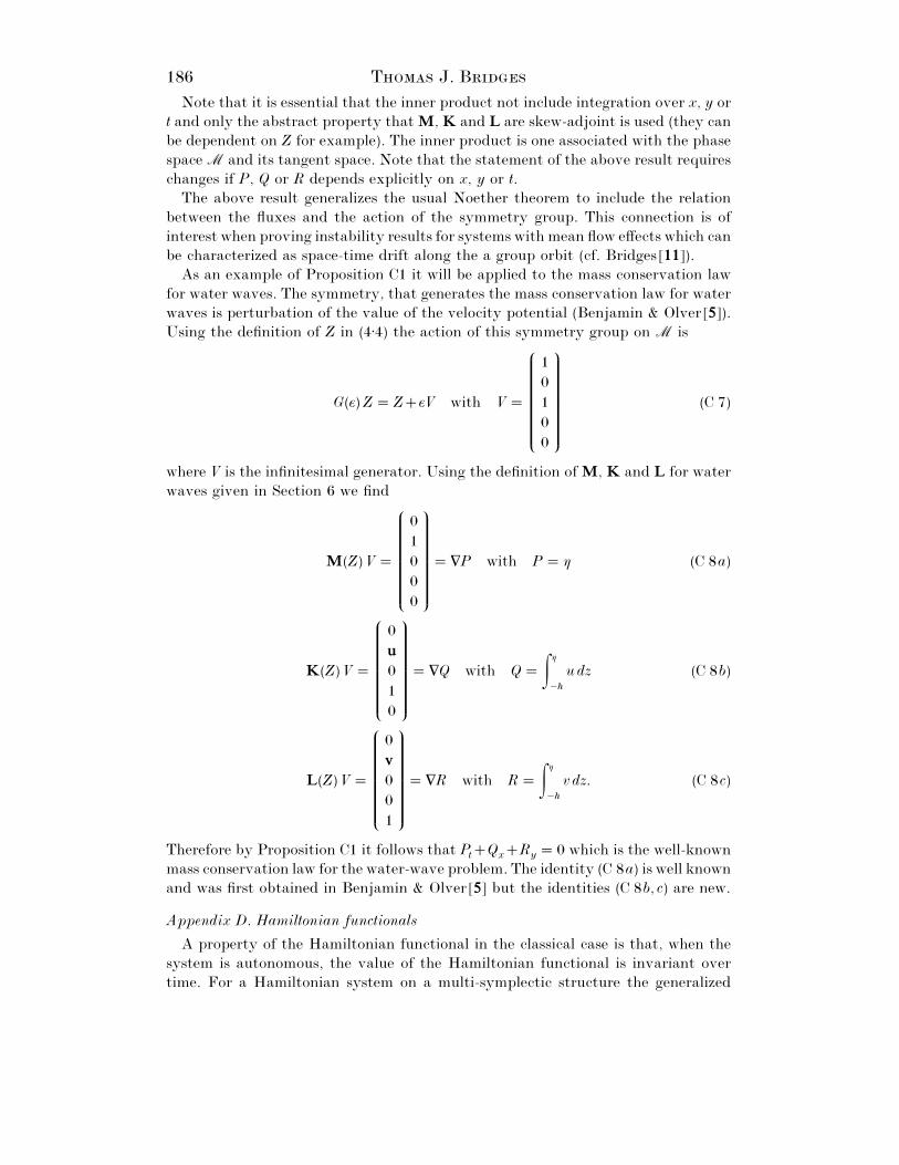
186 T J. B
Note that it is essential that the inner product not include integration over x, y or
t and only the abstract property that M, K and L are skew-adjoint is used (they can
be dependent on Z for example). The inner product is one associated with the phase
space - and its tangent space. Note that the statement of the above result requires
changes if P, Q or R depends explicitly on x, y or t.
The above result generalizes the usual Noether theorem to include the relation
between the fluxes and the action of the symmetry group. This connection is of
interest when proving instability results for systems with mean flow effects which can
be characterized as space-time drift along the a group orbit (cf. Bridges[11]).
As an example of Proposition C1 it will be applied to the mass conservation law
for water waves. The symmetry, that generates the mass conservation law for water
waves is perturbation of the value of the velocity potential (Benjamin & Olver[5]).
Using the definition of Z in (4±4) the action of this symmetry group on - is
G(ε)Z¯ZεV with V¯
E
F
1
0
1
0
0
G
H
(C 7)
where V is the infinitesimal generator. Using the definition of M, K and L for water
waves given in Section 6 we find
M(Z)V¯
E
F
0
1
0
0
0
G
H
¯~P with P¯ η (C 8a)
K(Z)V¯
E
F
0
u
0
1
0
G
H
¯~Q with Q¯&η
−h
udz (C 8b)
L(Z)V¯
E
F
0
v
0
0
1
G
H
¯~R with R¯&η
−h
v dz. (C 8c)
Therefore by Proposition C1 it follows that PtQ
xR
y¯ 0 which is the well-known
mass conservation law for the water-wave problem. The identity (C 8a) is well known
and was first obtained in Benjamin & Olver[5] but the identities (C 8b, c) are new.
Appendix D. Hamiltonian functionals
A property of the Hamiltonian functional in the classical case is that, when the
system is autonomous, the value of the Hamiltonian functional is invariant over
time. For a Hamiltonian system on a multi-symplectic structure the generalized
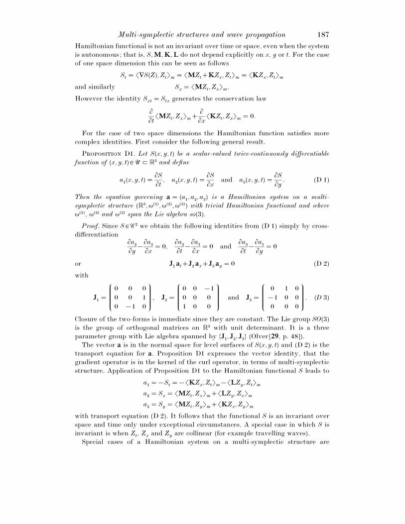
Multi-symplectic structures and wave propagation 187
Hamiltonian functional is not an invariant over time or space, even when the system
is autonomous; that is, S,M,K,L do not depend explicitly on x, y or t. For the case
of one space dimension this can be seen as follows
St¯©~S(Z),Z
tªm
¯©MZtKZ
x,Z
tªm
¯©KZx,Z
tªm
and similarly Sx¯©MZ
t,Z
xªm.
However the identity Sxt
¯Stx
generates the conservation law
¦¦t
©MZt,Z
xªm
¦¦x
©KZt,Z
xªm
¯ 0.
For the case of two space dimensions the Hamiltonian function satisfies more
complex identities. First consider the following general result.
P D1. Let S(x, y, t) be a scalar-valued twice-continuously differentiable
function of (x, y, t) `5Z2$ and define
a"(x, y, t)¯
¦S
¦t, a
#(x, y, t)¯
¦S
¦xand a
$(x, y, t)¯
¦S
¦y. (D 1)
Then the equation governing a¯ (a", a
#, a
$) is a Hamiltonian system on a multi-
symplectic structure (2$,ω("),ω(#),ω($)) with trivial Hamiltonian functional and where
ω("), ω(#) and ω($) span the Lie algebra so(3).
Proof. Since S `## we obtain the following identities from (D 1) simply by cross-
differentiation¦a
#
¦y®
¦a$
¦x¯ 0,
¦a#
¦t®
¦a"
¦x¯ 0 and
¦a$
¦t®
¦a"
¦y¯ 0
or J"atJ
#axJ
$ay¯ 0 (D 2)
with
J"¯
E
F
0
0
0
0
0
®1
1
0
0
G
H
, J#¯
E
F
0
0
1
0
0
0
0
®1
0
G
H
and J$¯
E
F
®1
0
0
0
1
0
0
0
0
G
H
. (D 3)
Closure of the two-forms is immediate since they are constant. The Lie group SO(3)
is the group of orthogonal matrices on 2$ with unit determinant. It is a three
parameter group with Lie algebra spanned by ²J", J
#, J
$´ (Olver[29, p. 48]).
The vector a is in the normal space for level surfaces of S(x, y, t) and (D 2) is the
transport equation for a. Proposition D1 expresses the vector identity, that the
gradient operator is in the kernel of the curl operator, in terms of multi-symplectic
structure. Application of Proposition D1 to the Hamiltonian functional S leads to
a"¯®S
t¯®©KZ
x,Z
tªm®©LZ
y,Z
tªm
a#¯S
x¯©MZ
t,Z
xªm©LZ
y,Z
xªm
a$¯S
y¯©MZ
t,Z
yªm©KZ
x,Z
yªm
with transport equation (D 2). It follows that the functional S is an invariant over
space and time only under exceptional circumstances. A special case in which S is
invariant is when Zt, Z
xand Z
yare collinear (for example travelling waves).
Special cases of a Hamiltonian system on a multi-symplectic structure are
188 T J. B
obtained as follows. For simplicity of discussion consider the system restricted to one
space dimension (-,ω("),ω(#),S) with governing equation
M(Z)ZtK(Z)Z
x¯~S(Z). (D 4)
The classic Hamiltonian structure for the system, denoted (-,ω("),Η), is recovered
by taking
MZt¯~H(Z,Z
x) with H(Z,Z
x)¯&x#
x"
[S(Z)®B(Z)] dx.
This corresponds to a classic Hamiltonian structure for the time-evolution equation
in terms of the larger set of corrdinates Z `-. The difficulty with analysing this
formulation when x `2 is that one must specify the function space over x. On the
other hand the roles of space and time can be reversed with the system (-,ω(#),Hh )with governing equation
KZx¯~Hh (Z,Z
t) with Hh (Z,Z
t)¯& t#
t"
[S(Z)®A(Z)] dt. (D 5)
In this case the function space over time (say periodic functions) is specified in
advance and then one seeks all bounded solutions (in x) of the spatial ‘evolution’
equation. A special case is the analysis of time-independent states with evolution
equation K(Z)Zx¯~S(Z).
A third possibility is to consider solutions of (D 4) that are stationary relative to
a moving frame. Let θ¯ x®ct then (D 4) becomes
(K®cM)Zθ ¯~S(Z). (D 6)
The Hamiltonian structure of spatial ‘evolution’ equations of the form (D 5)–(D 6)
are studied in Benjamin[3], Mielke[26], Baesens & MacKay[2] and Bridges[7,11].
For the system in (D 6) the functional S is an absolute spatial (θ) invariant,
¦θ S¯©~S(Z),Zθªm¯©(K®cM)Zθ,Zθªm
¯ 0
because K®cM is skew-symmetric and S in this case can be identified with the flow
force for the system.
The case of two-space dimensions (cf. (1±12)) contains further special cases with
evolution in various spatial directions. Finally we note that the family of symplectic
operators ω("),… ,ω(n) is, to be precise, a basis for the multi-symplectic structure.
For example one can introduce a non-degenerate linear transformation T taking
ω("),… ,ω(n) to a new basis Ω("),… ,Ω(n).
Acknowledgements. The research and writing of this work was partially carried out
while the author was supported by a Research Fellowship from the Alexander von
Humboldt Foundation held at the University of Stuttgart during the 1993–4
academic year.
REFERENCES
[1] D. G. A and M. E. MI. On wave-action and its relatives. J. Fluid Mech. 89(1978), 647–664.
[2] C. B and R. S. MK. Uniformly travelling water waves from a dynamical systemsviewpoint: some insights into bifurcations from Stokes’ family. J. Fluid Mech. 241 (1992),33–47.
Multi-symplectic structures and wave propagation 189
[3] T. B. B. Impulse, flow force and variational principles. IMA J. Applied Math. 32(1984), 3–68.
[4] T. B. B and J. E. F. The disintegration of wavetrains on deep water. Part 1.Theory, J. Fluid Mech. 27 (1967), 417–430.
[5] T. B. B and P. J. O. Hamiltonian structure, symmetries and conservation lawsfor water waves. J. Fluid Mech. 125 (1982), 137–185.
[6] D. J. B and G. J. R. Wave instabilities. Stud. Appl. Math. 48 (1969), 377–385.[7] T. J. B. Spatial Hamiltonian structure, energy flux and the water-wave problem. Proc.
Roy. Soc. London, Ser A 439 (1992), 297–315.[8] T. J. B. Hamiltonian bifurcations of the spatial structure for coupled nonlinear
Schro$ dinger equations. Physica D 57 (1992), 375–394.[9] T. J. B. Hamiltonian structure of plane wave instabilities, Fields Inst. Comm. 8
(1996), 19–33.[10] T. J. B. Hamiltonian spatial structure for three-dimensional water-waves in a moving
frame of reference. J. Nonlinear Science 4 (1994), 221–251.[11] T. J. B. Periodic patterns, linear instability, symplectic structure and mean-flow
dynamics for 3D surface waves. Philos. Trans. Roy. Soc. London, Ser. A 354 (1996),533–574.
[12] T. J. B. A geometric formulation of the conservation of wave action and itsimplications for signature and the classification of instabilities, preprint.
[13] T. J. B and A. M. A proof of the Benjamin–Feir instability. Arch. Rational Mech.Anal. 133 (1995), 145–198.
[14] T. J. B and G. R. Instability of spatially quasiperiodic states of theGinzburg–Landau equation. Proc. Roy. Soc. London, Ser. A 444 (1994), 347–362.
[15] L. J. F. B. On the Hamiltonian theory of surface waves. Appl. Sci. Res. 29 (1974),430–446.
[16] B. C and P. G. S. Three-dimensional stability and bifurcation of capillary andgravity waves on deep water. Stud. Appl. Math. 72 (1985), 125–147.
[17] R. G. Wave action and wave-mean flow interaction with application to stratifiedshear flows. Ann. Rev. Fluid Mech. 16 (1984), 11–44.
[18] W. D. H. Conservation of action and modal wave action. Proc. Roy. Soc. London Ser. A320 (1970), 187–208.
[19] W. D. H. Group velocity and nonlinear dispersive wave propagation. Proc. Roy. Soc.London Ser. A 332 (1973), 199–221.
[20] P. K. Floquet theory for partial differential equations (Birkha$ user, Verlag: Basel1993).
[21] M. J. L. Contributions to the theory of waves in nonlinear dispersive systems. J.Inst. Math. Appl. 1 (1965), 269–306.
[22] M. J. L. Some special cases treated by the Whitham theory. Proc. Roy. Soc. LondonSer. A 299 (1967), 28–53.
[23] R. S. MK and P. G. S. Stability of water waves. Proc. Roy. Soc. London Ser. A406 (1986), 115–125.
[24] J. H. M. On second-order conditions in constrained variational principles. J. Optim.Theory Appl., to appear.
[25] J. E. M. Applications of global analysis in mathematical physics, Math. Lect. Ser. 2(Publish or Perish, 1974).
[26] A. M. Hamiltonian and Lagrangian flows on center manifolds with applications to ellipticvariational problems. Lect. Notes in Math. 1489 (Springer-Verlag, 1991).
[27] P. K. N and J. B. K. Stability of periodic plane waves. SIAM J. Appl. Math. 47(1987), 959–964.
[28] P. J. O. On the Hamiltonian structure of evolution equations. Math. Proc. CambridgePhilos. Soc. 88 (1980), 71–88.
[29] P. J. O. Applications of Lie groups to differential equations. Graduate Texts in Math. 107(Springer-Verlag, 1986).
[30] I. C. P. Variational principles for the invariant toroids of classical dynamics. J. Phys.A : Math., Nucl. Gen. 7 (1974), 794–802.
[31] P. G. S. The superharmonic instability of finite-amplitude water waves. J. FluidMech. 159 (1985), 169–174.
[32] C. E. W. Periodic and quasiperiodic solutions of nonlinear wave equations via KAM theory.Comm. Math. Phys. 127 (1990), 479–528.

190 T J. B
[33] G. B. W. A general approach to linear and nonlinear dispersive waves using aLagrangian. J. Fluid Mech. 22 (1965), 273–283.
[34] G. B. W. Nonlinear dispersion of water-waves. J. Fluid Mech. 27 (1967), 399–412.[35] G. B. W. Linear and nonlinear waves (Wiley-Interscience, 1974).[36] V. E. Z. Stability of periodic waves of finite amplitude on the surface of a deep fluid.
Zh. Prikl. Mekh. Fiz. 9 (1968), 86–94 (English trans: J. Appl. Mech. Tech. Phys. 2 (1968),190).


