
Monroe L. Weber-Shirk School of Civil and
Environmental Engineering
Viscous Flow in PipesViscous Flow in Pipes
CEE 331 Fluid Mechanics
April 18, 2023

Types of Engineering Problems
How big does the pipe have to be to carry a flow of x m3/s?
What will the pressure in the water distribution system be when a fire hydrant is open?
Can we increase the flow in this old pipe by adding a smooth liner?

Viscous Flow in Pipes: Overview
Boundary Layer DevelopmentTurbulenceVelocity DistributionsEnergy LossesMajorMinor
Solution Techniques

Transition at Re of 2000
Laminar and Turbulent Flows
Reynolds apparatus
ReVDrm
= =dampinginertia

Boundary layer growth: Transition length
What does the water near the pipeline wall experience? _________________________Why does the water in the center of the pipeline speed up? _________________________
v v
Drag or shear
Conservation of mass
Non-Uniform Flow
v

Entrance Region Length
1
10
100
Re
l e /D
1/ 64.4 Reel
D0.06Reel
D
laminar turbulent
Reel fD
Distance for velocity profile to develop
Shear in the entrance region vs shear in long pipes?
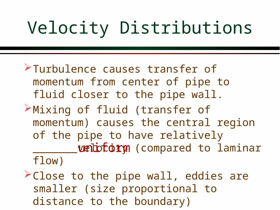
Velocity Distributions
Turbulence causes transfer of momentum from center of pipe to fluid closer to the pipe wall.
Mixing of fluid (transfer of momentum) causes the central region of the pipe to have relatively _______velocity (compared to laminar flow)
Close to the pipe wall, eddies are smaller (size proportional to distance to the boundary)
uniform
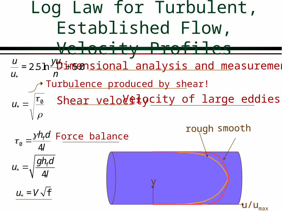
Shear velocity
Dimensional analysis and measurements
Velocity of large eddies
Log Law for Turbulent, Established Flow, Velocity Profiles
*
*
2.5ln 5.0u yuu n= +
0* u
u/umax
rough smooth
y
f0 4
h d
l
f* 4
gh du
l
Force balance
Turbulence produced by shear!
* fu V=
Pipe Flow: The Problem
We have the control volume energy equation for pipe flow
We need to be able to predict the head loss term.
We will use the results we obtained using dimensional analysis
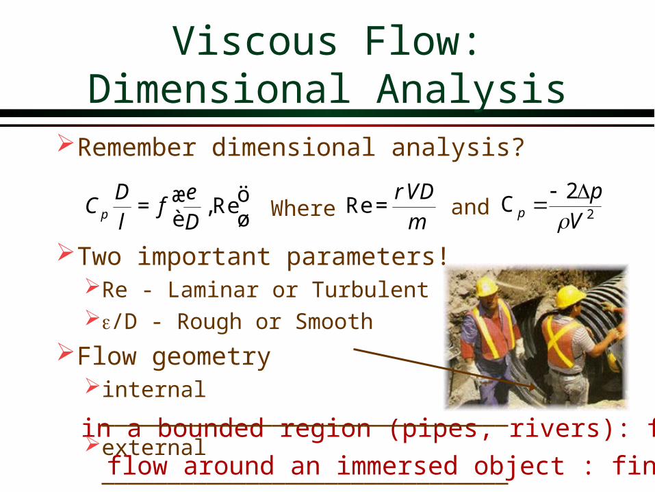
,Rep
DC f
l Deæ ö=è ø 2
2C
Vp
p Re
VDrm
=
Viscous Flow: Dimensional Analysis
Where and
in a bounded region (pipes, rivers): find Cp
flow around an immersed object : find Cd
Remember dimensional analysis?
Two important parameters!Re - Laminar or Turbulent/D - Rough or Smooth
Flow geometryinternal _______________________________external _______________________________
Dimensional Analysis
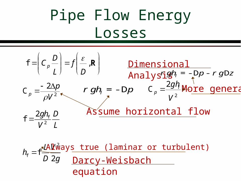
Darcy-Weisbach equation
Pipe Flow Energy Losses
R,f
Df
L
DC p
2
2C
Vp
p
2
2C
V
ghlp
f2
2f
gh D
V L
2
f f2
L Vh
D g
lgh pr =- D
Always true (laminar or turbulent)
Assume horizontal flow
More general
lgh p g zr r=- D - D

Friction Factor : Major losses
Laminar flowTurbulent (Smooth, Transition, Rough) Colebrook FormulaMoody diagramSwamee-Jain

Hagen-Poiseuille
Darcy-Weisbach
Laminar Flow Friction Factor
2
32lhgD
VL
rm
=
f 2
32 LVh
gD
2
f f2
L Vh
D g
gV
DL
gDLV
2f
32 2
2
RVD6464
f
Slope of ___ on log-log plot-1
fh V
f independent of roughness!

Turbulent Flow:Smooth, Rough, Transition
Hydraulically smooth pipe law (von Karman, 1930)
Rough pipe law (von Karman, 1930)
Transition function for both smooth and rough pipe laws (Colebrook)
1 Re f2log
2.51f
æ ö= ç ÷è ø
1 3.72log
f
De
æ ö=è ø
2
f f2
L Vh
D g
(used to draw the Moody diagram)
1 2.512log
3.7f Re f
Deæ ö=- +è ø
*fu
V

Moody Diagram
0.01
0.10
1E+03 1E+04 1E+05 1E+06 1E+07 1E+08Re
fric
tion
fact
or
laminar
0.050.04
0.03
0.020.015
0.010.0080.006
0.004
0.002
0.0010.0008
0.0004
0.0002
0.0001
0.00005
smooth
lD
C pf
D
0.02
0.03
0.04
0.050.06
0.08
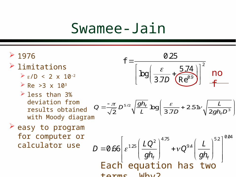
Swamee-Jain
1976 limitations
/D < 2 x 10⁻²
Re >3 x 10³
less than 3% deviation from results obtained with Moody diagram
easy to program for computer or calculator use
0.044.75 5.221.25 9.4
f f
0.66LQ L
D Qgh gh
2
0.9
0.25f
5.74log
3.7 ReD
no f
Each equation has two terms. Why?
5/ 2 f3
f
log 2.513.7 22
gh LQ D
L D gh D

Pipe roughness
pipe material pipe roughness (mm)
glass, drawn brass, copper 0.0015
commercial steel or wrought iron 0.045
asphalted cast iron 0.12
galvanized iron 0.15
cast iron 0.26
concrete 0.18-0.6
rivet steel 0.9-9.0
corrugated metal 45PVC 0.12
d Must be
dimensionless!
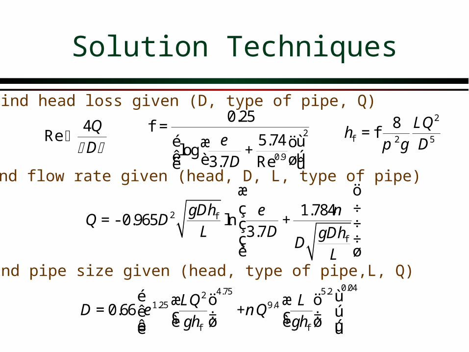
find head loss given (D, type of pipe, Q)
find flow rate given (head, D, L, type of pipe)
find pipe size given (head, type of pipe,L, Q)
Solution Techniques
2 f
f
1.7840.965 ln
3.7gDh
Q DL D gDh
DL
e næ öç ÷
=- +ç ÷ç ÷è ø
0.044.75 5.221.25 9.4
f f
0.66LQ L
D Qgh gh
e né ùæ ö æ ö
= +ê úç ÷ ç ÷è ø è øê úë û
2
f 2 5
8f
LQh
g Dp=2
0.9
0.25f
5.74log
3.7 ReDe
=é ùæ ö+ê úè øë û
Re 4QD

Example: Find a pipe diameter
The marine pipeline for the Lake Source Cooling project will be 3.1 km in length, carry a maximum flow of 2 m3/s, and can withstand a maximum pressure differential between the inside and outside of the pipe of 28 kPa. The pipe roughness is 2 mm. What diameter pipe should be used?
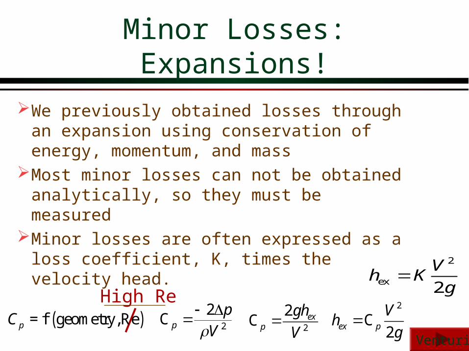
Minor Losses: Expansions!
We previously obtained losses through an expansion using conservation of energy, momentum, and mass
Most minor losses can not be obtained analytically, so they must be measured
Minor losses are often expressed as a loss coefficient, K, times the velocity head.
2
ex 2
Vh K
g
( )f geometry,RepC = 2
2C
Vp
p
2
2C ex
p
gh
V
2
C2ex p
Vh
g
Venturi
High Re

Sudden Contraction
V1 V2
EGL
HGL
vena contracta Losses are reduced with a gradual contraction Equation has same form as expansion equation!
g
V
Ch
c
c
21
1 22
2
2A
AC c
c
0.60.650.7
0.750.8
0.850.9
0.951
0 0.2 0.4 0.6 0.8 1
A2/A1
Cc
0.60.650.7
0.750.8
0.850.9
0.951
0 0.2 0.4 0.6 0.8 1
A2/A1
Cc
0.60.650.7
0.750.8
0.850.9
0.951
0 0.2 0.4 0.6 0.8 1
A2/A1
Cc
c 2
22
ex 12
in in
out
V Ah
g A
Prove this!

g
VKh ee
2
2
0.1eK
5.0eK
04.0eK
Entrance Losses
Losses can be reduced by accelerating the flow gradually and eliminating thevena contracta
Estimate based on contraction equations!

Head Loss in Bends
Head loss is a function of the ratio of the bend radius to the pipe diameter (R/D)
Velocity distribution returns to normal several pipe diameters downstream
High pressure
Low pressure
Possible separation from wall
D
R
g
VKh bb
2
2
Kb varies from 0.6 - 0.9
2Vp dn z Cr g+ + =ó
ôõ R
n
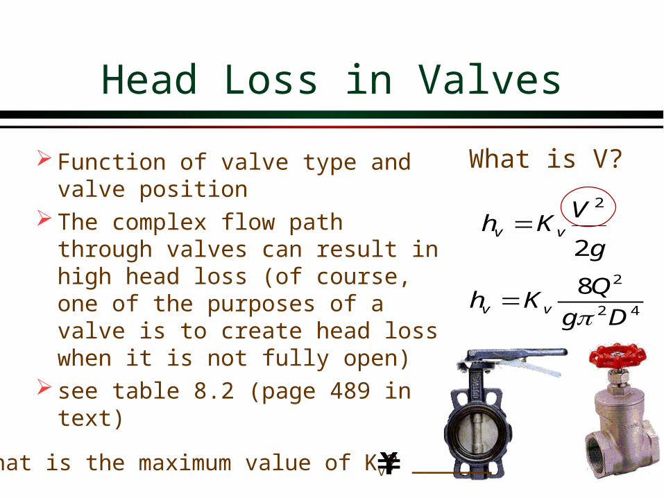
Head Loss in Valves
Function of valve type and valve position
The complex flow path through valves can result in high head loss (of course, one of the purposes of a valve is to create head loss when it is not fully open)
see table 8.2 (page 489 in text)
g
VKh vv
2
2
What is the maximum value of Kv? ______¥
2
2 4
8v v
Qh K
g D
What is V?
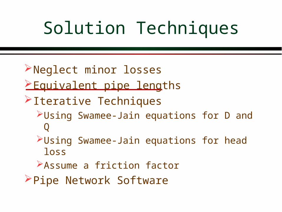
Solution Techniques
Neglect minor lossesEquivalent pipe lengthsIterative TechniquesUsing Swamee-Jain equations for D and QUsing Swamee-Jain equations for head lossAssume a friction factor
Pipe Network Software

Solution Technique 1: Find D or Q
Assume all head loss is major head lossCalculate D or Q using Swamee-Jain
equationsCalculate minor lossesFind new major losses by subtracting minor
losses from total head loss 0.044.75 5.22
1.25 9.4
f f
0.66LQ L
D Qgh gh
e né ùæ ö æ ö
= +ê úç ÷ ç ÷è ø è øê úë û
2
2 4
8ex
Qh K
g D
f l exh h h
5/ 2 f3
f
log 2.513.7 22
gh LQ D
L D gh D

Solution Technique: Head Loss
Can be solved explicitly
fl minorh h h= +å å
2
2minor
Vh K
g=å
2
f 2 5
8f
LQh
g Dp=
2
9.0Re
74.5
7.3log
25.0
D
f
2
2 4
8minor
Q Kh
g Dp= å
D
Q4Re

Solution Technique 2:Find D or Q using Solver
Iterative techniqueSolve these equations
fl minorh h h= +å å
42
28
Dg
QKhminor
2
f 2 5
8f
LQh
g Dp=2
0.9
0.25f
5.74log
3.7 ReDe
=é ùæ ö+ê úè øë ûD
Q4Re
Use goal seek or Solver to find discharge that makes the calculated head loss equal the given head loss.
Spreadsheet
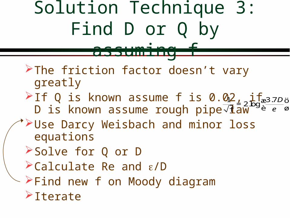
Solution Technique 3:Find D or Q by assuming f
The friction factor doesn’t vary greatlyIf Q is known assume f is 0.02, if D is
known assume rough pipe lawUse Darcy Weisbach and minor loss
equationsSolve for Q or DCalculate Re and /DFind new f on Moody diagramIterate
1 3.72log
f
De
æ ö=è ø
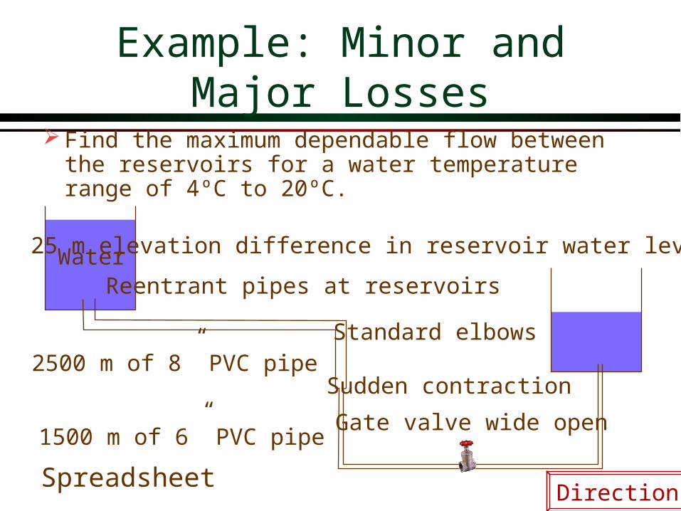
Example: Minor and Major Losses
Find the maximum dependable flow between the reservoirs for a water temperature range of 4ºC to 20ºC.
Water
2500 m of 8” PVC pipe
1500 m of 6” PVC pipeGate valve wide open
Standard elbows
Reentrant pipes at reservoirs
25 m elevation difference in reservoir water levels
Sudden contraction
DirectionsSpreadsheet
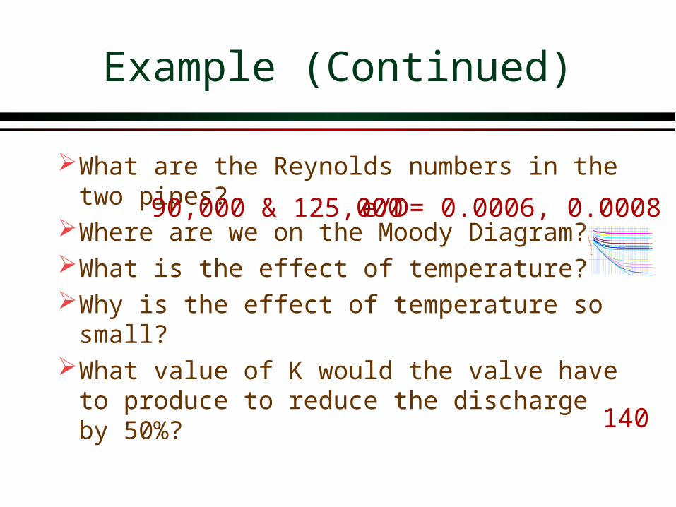
Example (Continued)
What are the Reynolds numbers in the two pipes?
Where are we on the Moody Diagram?What is the effect of temperature?Why is the effect of temperature so small?What value of K would the valve have to
produce to reduce the discharge by 50%?
0.01
0.1
1E+03 1E+04 1E+05 1E+06 1E+07 1E+08Re
fric
tion
fact
or
laminar
0.050.04
0.03
0.020.015
0.010.0080.006
0.004
0.002
0.0010.0008
0.0004
0.0002
0.0001
0.00005
smooth
90,000 & 125,000
140
e/D= 0.0006, 0.0008

Example (Continued)
Were the minor losses negligible?Accuracy of head loss calculations?What happens if the roughness increases by
a factor of 10?If you needed to increase the flow by 30%
what could you do?
0.01
0.1
1E+03 1E+04 1E+05 1E+06 1E+07 1E+08Re
fric
tion
fact
or
laminar
0.050.04
0.03
0.020.015
0.010.0080.006
0.004
0.002
0.0010.0008
0.0004
0.0002
0.0001
0.00005
smooth
Yes
5%
f goes from 0.02 to 0.035
Increase small pipe diameter

Pipe Flow Summary (1)
linearly
experimental
Shear increases _________ with distance from the center of the pipe (for both laminar and turbulent flow)
Laminar flow losses and velocity distributions can be derived based on momentum (Navier Stokes) and energy conservation
Turbulent flow losses and velocity distributions require ___________ results

Pipe Flow Summary (2)
Energy equation left us with the elusive head loss term
Dimensional analysis gave us the form of the head loss term (pressure coefficient)
Experiments gave us the relationship between the pressure coefficient and the geometric parameters and the Reynolds number (results summarized on Moody diagram)
Pipe Flow Summary (3)
Dimensionally correct equations fit to the empirical results can be incorporated into computer or calculator solution techniques
Minor losses are obtained from the pressure coefficient based on the fact that the pressure coefficient is _______ at high Reynolds numbers
Solutions for discharge or pipe diameter often require iterative or computer solutions
constant

Pipes are Everywhere!
Owner: City of Hammond, INProject: Water Main RelocationPipe Size: 54"

Pipes are Everywhere!Drainage Pipes
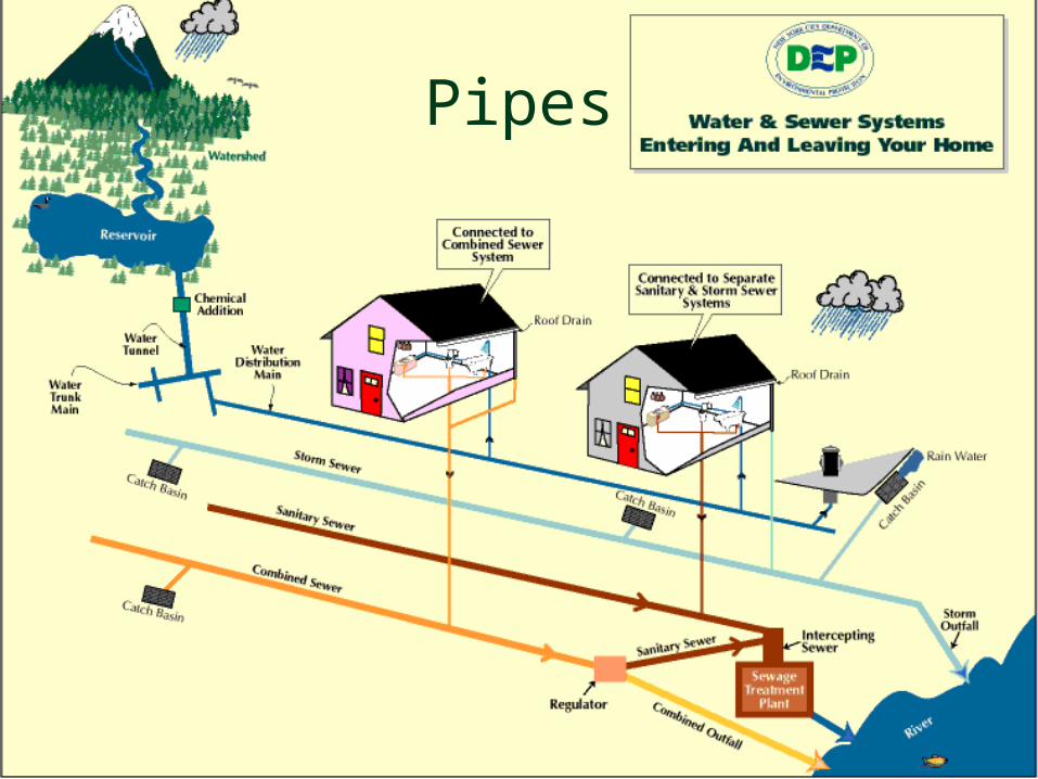
Pipes
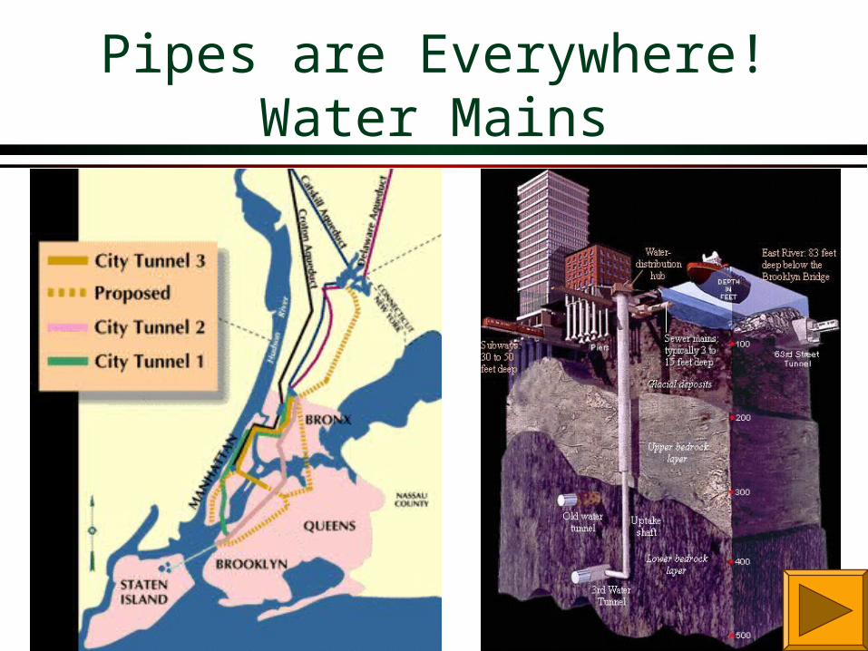
Pipes are Everywhere!Water Mains
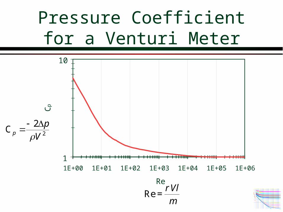
Pressure Coefficient for a Venturi Meter
1
10
1E+00 1E+01 1E+02 1E+03 1E+04 1E+05 1E+06
Re
Cp
ReVlrm
=
2
2C
Vp
p
0.01
0.1
1E+03 1E+04 1E+05 1E+06 1E+07 1E+08Re
fric
tion
fact
or
laminar
0.050.04
0.03
0.020.015
0.010.0080.006
0.004
0.002
0.0010.0008
0.0004
0.0002
0.0001
0.00005
smooth

Moody Diagram
0.01
0.1
1E+03 1E+04 1E+05 1E+06 1E+07 1E+08Re
fric
tion
fact
or
laminar
0.050.04
0.03
0.020.015
0.010.0080.006
0.004
0.002
0.0010.0008
0.0004
0.0002
0.0001
0.00005
smooth
lD
C pf
D
Minor Losses

LSC Pipeline
cs1
cs2
2 21 1 2 2
1 1 2 22 2 l e
p V p Vz z h h
g g
z = 0
Ignore entrance losses
≈0
28 kPa is equivalent to 2.85 m of water-2.85 m
D m 154.
DLQgh
QL
ghf f
FHGIKJ
FHGIKJ
LNMM
OQPP0 66 1 25
24 75
9 4
5 2 0 04
. .
.
.
. .
Q m s
m s
L m
m
h mf
2
10
3100
0 002
2 85
3
6 2
/
/
.
.
1.07 /V m s

Directions
Assume fully turbulent (rough pipe law)find f from Moody (or from von Karman)
Find total head loss (draw control volume)Solve for Q using symbols (must include
minor losses) (no iteration required)
0.01
0.1
1E+03 1E+04 1E+05 1E+06 1E+07 1E+08Re
fric
tion
fact
or
laminar
0.050.04
0.03
0.020.015
0.010.0080.006
0.004
0.002
0.0010.0008
0.0004
0.0002
0.0001
0.00005
smooth
Pipe roughness
fl minorh h h= +å å Solution
WaterWater

Find Q given pipe system
fl minorh h h= +å å
42
28
Dg
QKhminor
2
2 5
8ff
LQh
g Dp=
2
2 5 4
8fl
Q L Kh
g D Dpé ùæ ö æ ö= +ê úè ø è øë ûå å
5 48 f
lghQ
L KD D
p=é ùæ ö æ ö+ê úè ø è øë ûå å
WaterWater


