
MODELLING A LOW COST, DATA ACQISITION AND IRRIGATION SEQUENCING
SYSTEM FOR A GREENHOUSE ON AN 8 BIT PIC MICROCONTROLLER
A thesis submitted in partial fulfillment of the requirements of the requirements for the
award of Degree in Computer Science
Master of Science in computer Science
BY
Author: Hilton Chikwiriro
Under the supervision of
Mr M Munyaradzi( Lecturer)
And
Mr E Mashonjowa(Lecturer, UZ Physics Departemnt)
University Of Zimbabwe
Department of Computer Science
Faculty of Science

ii
Abstract
The debate on climate change is still going on and on, and there is still no convincing evidence
that greenhouse gases are the real, real cause of the recent changes in climate patterns. Some
records tend to suggest that the climate change that is taking place is a normal cycle. However
with the ever increasing world population, we cannot be to sure about the future of food and
water.
A variety of Water use efficiency methods have been proposed, but most of them have been
found to be very expensive and complicated to use. In future each and every farmer, whether
poor or uneducated might wake up in need of such a system, therefore the proposed applications
need minimal cost components, less powerful controllers, minimal human-computer interaction.
This thesis presents a strategy to provide a computer-less Irrigation control system, which uses a
cheap 8 bit, low processing power, small working memory and small storage capacity PIC
Microcontroller which requires minimal human-computer interaction, uses a single sensor and
low electrical power.

iii
Acknowledgements
Firstly I would like to thank the Lord for everything he has done for me in my life and his unconditional love. All the honour and glory goes to you. Special thanks go to my supervisors Mr Munyaradzi and Mr mashonjowa, who gave me an opportunity to work with them and explore the field of Micro-computing in Agriculture. Thank you for all the encouragement, guidance, help and support. Let me also take this opportunity to express my gratitude to my, twin brother Hilary, my mother, my sisters, and my brothers for their strong encouragement and support.
Finally I would like to thank all the staff at the Computer Science department, my friends from the MSc Computer Science class and around the world, Mr Chipindu, Dr Mhizha, Mr Simba and Mr Grey all from the Physics department and lastly Dr Carelse and Mr Chirere from the SIRDC.
l dedicate this research to the brave men and women of the Columbia space shuttle , the last crew
of astronauts to perish inside a space shuttle , who perished on the 1st of July 2003 after re-entry
into the earth’s atmosphere, 16 minutes before the scheduled landing time. Crew members (All
from the NASSA space center in Washington DC and J.F Kennedy space center in Miami)
Mr David M Brown
Mr Rick D Husband (Head space shuttle crew)
Mrs Laurel B Clark
Dr Kalpana Chalwa (Mrs)
Mr Michael P Anderson
Mr Han Ramon
Mr William C McCool
We shall always remember you all for your dedication, for your determination, for your courage
and for the knowledge and pride that you brought to our earth. May their souls rest in eternal
peace.

iv
Table of contents
Table of contents ............................................................................................................................... iv
List of Figures ......................................................................................................................................... vi
List of tables .......................................................................................................................................... vii
List of Annexes ...................................................................................................................................... vii
Chapter 1 ................................................................................................................................................ 2
Background and justification ............................................................................................................... 2
1.0 Introduction ............................................................................................................................... 2
1.1 Problem statement .................................................................................................................... 3
1.2 Aims and objectives ................................................................................................................... 4
1.3 Expected benefits ...................................................................................................................... 4
1.4 Thesis layout .............................................................................................................................. 4
Chapter 2 ................................................................................................................................................ 5
Literature review ................................................................................................................................. 5
2.0 Introduction ............................................................................................................................... 5
2.1 Water use and management in agriculture .............................................................................. 6
2.2 Irrigation scheduling ................................................................................................................. 8
2.3 Irrigation scheduling techniques ............................................................................................... 8
2.4 Irrigation Control Systems ........................................................................................................ 38
2.5 Computer-Based Irrigation Control Systems ............................................................................. 42
2.6 Computer-based Controller Topologies .................................................................................... 47
2.7 Controllers ............................................................................................................................... 48
Chapter 3 .............................................................................................................................................. 55
Materials and Methodology............................................................................................................... 55

v
3.0 Introduction ............................................................................................................................. 55
The following materials were used in this project: ............................................................................. 55
3.1 The PIC 16F872 Microcontroller ............................................................................................... 55
3.2 CM 3 Pyranometer, .................................................................................................................. 57
3.3 System physical design ............................................................................................................. 58
3.4 Data acquisition ....................................................................................................................... 59
3.5 Data Processing and Irrigation sequencing ............................................................................... 63
Chapter 4 .............................................................................................................................................. 66
Conclusions, recommendations and future work ............................................................................... 66
4.0 Conclusions .............................................................................................................................. 66
4.1 Recommendations ................................................................................................................... 67
4.2 Future work ............................................................................................................................. 67
REFERENCES .................................................................................................................................. 68
Annexes ................................................................................................................................................ 73
vi
List of Figures
Fig. 2.0 Major climatic factors influencing crop water needs ........................................... 5
Fig. 2.1 Reference crop evapotranspiration ..................................................................... 6
Fig. 2.3 Pan Evaporation method ................................................................................... 21
Fig. 2.4a Class A evaporation pan .................................................................................. 22
Fig. 2.4b Sunken Colorado pan ....................................................................................... 22
figure 2.5 Illustration of the effect of wind speed on evapotranspiration...................... 25
Fig. 2.6 The Blaney-Criddle method ............................................................................... 36
Figure 2.7b shows a closed loop system in its simplest form ......................................... 41
Figure 2.8 basic components of a closed loop control system ....................................... 43
Figure 2.9 an example of a continuous sensor ............................................................... 44
Figure 2.11 a typical commercially available electromechanical controller .................. 49
Figure 2.12 shows a typical commercially available electronic controller ...................... 50
Fig 3.0 PIC16F872 Microcontroller ................................................................................. 55
Fig 3.1 Irrigation System’s physical design ..................................................................... 58
Fig 3.2 Irrigation systems power supply unit .................................................................. 59
Fig 3.3 Irrigation system’s display unit ........................................................................... 60
Fig 3.4 Irrigation system’s relay unit .............................................................................. 61
Fig 3.3 Irrigation system’s electronic circuit ................................................................... 62

vii
List of tables
Table 2.1 Some PIC 12CXXX family members ............................................................. 51
Table 2.2 Some PIC16C5X family members ................................................................ 52
Table 2.3 Some PIC16CXXX and PIC16FXXX family members ..................................... 53
Table 2.4 Some PIC17CXXX and PIC18CXXX family members ..................................... 54
List of Annexes
Annex A .................................................................................................................. 73
Annex B .................................................................................................................. 73
Annex C .................................................................................................................. 75
Annex D .................................................................................................................. 78

2
Chapter 1
Background and justification
1.0 Introduction
According to IPCC (2007a:10), It is predicted that future climate changes will include further
global warming (i.e., an upward trend in global mean temperature), sea level rise, and a probable
increase in the frequency of some extreme weather events. Some areas of the earth will become
wetter, while most areas will experience heavy droughts. According to the Intergovernmental
Panel on Climate, Africa, where water is already a scarce commodity, will have less and less
water with warmer temperatures.
However, according to the capitalist magazine, the Earth's warming since 1850 totals about 0.7
degrees Celsius. Most of this occurred before 1940. The cause was a long, moderate 1,500-year
climate cycle first discovered in the Greenland ice cores in 1983. The cycle abruptly raises our
temperature 1 to 3 degrees C above the mean for centuries at a time--as it did during the Roman
Warming (200 BC to 600 AD) and Medieval Warming (950 to1300 AD).Between warmings,
Earth's temperatures shift abruptly lower by 1 to 3 degrees C--as they did during the 550 years of
the Little Ice Age, which ended in 1850. The ice cores and seabed fossils show 600 of these
1,500-year cycles, extending back at least 1 million years.
In Al Gore's movie, the ice record from the Antarctic shows temperatures and atmospheric CO2
levels tracking closely together through the radical ups and downs of four Ice Ages. The movie
implies that more CO2 in the air produces higher temperatures, but recently done, more refined
ice studies show that temperatures changed about 800 years before the CO2 levels. More CO2 did
not produce higher temperatures; instead, higher temperatures released more CO2 from the
oceans into the atmosphere. If the climate models' original greenhouse predictions had been
valid, the Earth's temperatures would have risen several degrees more by now than they have.

3
The Earth's net warming since 1940 is a barely noticeable 0.2 degrees C, over 70 years.
Moreover, the Earth has experienced no discernible temperature increase since 1998, nearly nine
years ago. Remember, too, that the atmosphere is approaching CO2 saturation--after which more
CO2 will have no added climate forcing power.
"There is no convincing scientific evidence that human release of carbon dioxide, methane, or
other greenhouse gasses is causing, or will, in the foreseeable future, cause catastrophic heating
of the Earth's atmosphere and disruption of the Earth's climate." That statement comes from a
petition signed by more than 19,000 American scientists, available online at a site hosted by the
Oregon Institute for Science and Medicine at www.oism.org. However, the absence of evidence
is not the evidence of the absence of evidence. No one can be pretty sure what our climate will
be like in 25, 50, or 100 years. You could be standing in a future desert or a future ocean. One
thing is certain, though, our planet as a whole will be a lot better off if we can stabilize global
carbon output.
Irrigation scheduling has conventionally aimed to achieve an optimum water supply for
productivity, with soil water content being maintained close to field capacity. The increasing
worldwide shortages of water and costs of irrigation are leading to an emphasis on developing
methods of irrigation that minimize water use (maximize the water use efficiency).
1.1 Problem statement
Although there exists many methods for data acquisition and irrigation sequencing, each of these
methods is very expensive and beyond the reach of many farmers. Most methods require that a
farmer must have some of the following:
- a computer
- several sensory devices
- networking devices to transmit signals
- knowledge of his soil properties

4
- knowledge of plant properties
1.2 Aims and objectives
i) Develop an irrigation sequencing algorithm based on Agro-Meteorological data and
equation
ii) Design an algorithm for irrigation sequencing
iii) Design and development of an appropriate automated irrigation control system.
1.3 Expected benefits
i) Increased water use efficiency for low to average income farmers
ii) Reduced user-computer interaction
1.4 Thesis layout
The thesis is organized in the following way:
Chapter 1 (Introduction):
This chapter introduces the research topic and sets the direction in which the thesis will
proceed.
Chapter 2 (Literature Review):
A review of all the information that is relevant to the research.
Chapter 3 (Methodology):
In this chapter the proposed solution is presented. It is explained and analysis of Circuits
and algorithm is made.
Chapter 4 (Conclusion)
This chapter gives the conclusions drawn from the research and its results as well as
recommendations on future work that can be done.
5
Chapter 2
Literature review
2.0 Introduction
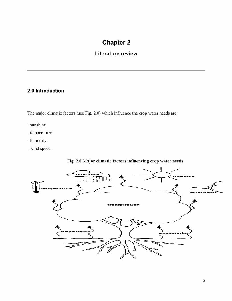
The major climatic factors (see Fig. 2.0) which influence the crop water needs are:
- sunshine
- temperature
- humidity
- wind speed
Fig. 2.0 Major climatic factors influencing crop water needs

6
The highest crop water needs are thus found in areas which are hot, dry, windy and sunny. The
lowest values are found when it is cool, humid and cloudy with little or no wind.
2.1 Water use and management in agriculture
2.1.1 Evapotranspiration
The influence of the climate on crop water needs is given by the reference crop
evapotranspiration (ETo). The ETo is usually expressed in millimetres per unit of time, e.g.
mm/day, mm/month, or mm/season. Grass has been taken as the reference crop. ETo is the rate
of evapotranspiration from a large area, covered by green grass, 8 to 15 cm tall, which grows
actively, completely shades the ground and which is not short of water.
Fig. 2.1 Reference crop evapotranspiration

7
There are several methods to determine the ETo . They are either:
ü experimental, using an evaporation pan, or
ü theoretical, using measured climatic data, e.g. the Blaney-Criddle method
2.1.2 Crop water requirements
The crop water need (ET crop) is defined as the depth (or amount) of water needed to meet the
water loss through evapotranspiration. In other words, it is the amount of water needed by the
various crops to grow optimally. The crop water need always refers to a crop grown under
optimal conditions, i.e. a uniform crop, actively growing, completely shading the ground, free of
diseases, and favourable soil conditions (including fertility and water). The crop thus reaches its
full production potential under the given environment.
The crop water need mainly depends on:
ü the climate: in a sunny and hot climate crops need more water per day than in a cloudy
and cool climate
ü the crop type: crops like maize or sugarcane need more water than crops like millet or
sorghum
ü the growth stage of the crop; fully grown crops need more water than crops that have just
been planted.

8
2.2 Irrigation scheduling
The advent of precision irrigation methods such as trickle irrigation has played a major role in
reducing the water required in agricultural and horticultural crops, but has highlighted the need
for new methods of accurate irrigation scheduling and control.
The choice of irrigation scheduling method depends to a large degree on the objectives of the
irrigator and the irrigation system available. The more sophisticated scheduling methods
generally require higher-precision application systems; nevertheless even less sophisticated
systems such as flood irrigation scheduling can benefit from improvements in irrigation
scheduling as outlined here. The pressures to improve irrigation use efficiency and to use
irrigation for precise control of vegetative growth both imply a requirement for increased
precision in irrigation control, maintaining the soil moisture status within fine bands to achieve
specific objectives in crop management. Such objectives can only be met by precision irrigation
systems such as trickle irrigation that can apply precise amounts of water at frequent intervals
(often several times per day). Effective operation of such systems equally requires a sensing
system that determines irrigation need in real time or at least at frequent intervals; this rules out
large-scale manual monitoring programmes for such purposes and indicates a need for automated
monitoring systems.
2.3 Irrigation scheduling techniques
Irrigation scheduling is conventionally based either on ‘soil water measurement’, where the soil
moisture status (whether in terms of water content or water potential) is measured directly to
determine the need for irrigation, or on ‘soil water balance calculations’, where the soil moisture
status is estimated by calculation using a water balance approach in which the change in soil
moisture ( ) over a period is given by the difference between the inputs (irrigation plus
precipitation) and the losses (runoff plus drainage plus evapotranspiration).
A potential problem with all soil-water based approaches is that many features of the plant's
physiology respond directly to changes in water status in the plant tissues, whether in the roots or
in other tissues, rather than to changes in the bulk soil water content (or potential). The actual
9
tissue water potential at any time therefore depends both on the soil moisture status and on the
rate of water flow through the plant and the corresponding hydraulic flow resistances between
the bulk soil and the appropriate plant tissues. The plant response to a given amount of soil
moisture therefore varies as a complex function of evaporative demand. As a result it has been
suggested (Jones, 1990a) that greater precision in the application of irrigation can potentially be
obtained by a third approach, the use of ‘plant "stress" sensing’. For this approach irrigation
scheduling decisions are based on plant responses rather than on direct measurements of soil
water status.
Although the water balance approach is not very accurate, it has generally been found to be
sufficiently robust under a wide range of conditions. Nevertheless it is subject to the serious
problem that errors are cumulative over time. For this reason it is often necessary to recalibrate
the calculated water balance at intervals by using actual soil measurements, or sometimes plant
response measurements.
2.3.1 Plant-based methods for irrigation control
If soil water-based measures are to be replaced by plant-based measures it is important to
consider what measures might be most appropriate for irrigation scheduling purposes. Possible
measures include direct measurements of some aspect of plant water status as well as
measurements of a number of plant processes that are known to respond sensitively to water
deficits. One might expect that a direct measure of plant water status should be the most rigorous
and hence the most useful indicator of irrigation requirement, although the question remains as to
where in the plant that quantity should be measured. In practice, as has been argued strongly by
Jones (1990b), most plants exercise some measure of autonomous control over their shoot or leaf
water status, tending to minimize changes in shoot water status as the soil dries or as evaporative
demand increases (Bates and Hall, 1981; Jones, 1983). In the long term, this control is achieved
through changes in leaf area and root extension, and in the shorter term through changes in leaf
angle, stomatal conductance, and hydraulic properties of the transport system. In extreme cases,
plants with good endogenous control systems maintain a stable leaf water status over a wide
range of evaporative demand or soil water supplies; these plants are termed ‘isohydric’ (Stocker,

10
1956), and include especially plants such as cowpea, maize, and poplar (Bates and Hall, 1981;
Tardieu and Simonneau, 1998). This is by contrast with those species such as sunflower or barley
which appear to have less effective control of leaf water status and have been termed
‘anisohydric’. In practice the distinctions between isohydric and anisohydric behaviour are often
not clear-cut; even different cultivars of grapevine have been shown to have contrasting
hydraulic behaviours (Schultz, 2003).
The choice of which plant-based measure to use depends on their relative sensitivity to water
deficits. The definition of sensitivity, however, is somewhat problematic. The relative
sensitivities of different physiological processes were reviewed in some detail by Hsiao (1973),
who identified cell growth as being most sensitive to tissue water deficits, closely followed by
wall and protein synthesis, all of which could respond to water deficits of less than 0.1 MPa.
Hsiao reported that stomatal closure was only rarely affected when tissue water potential fell by
0.2–0.5 MPa, with decreases of 1.0 MPa or more being required for stomatal closure in many
cases. Although photosynthesis was classified as moderately sensitive by Hsiao, largely as a
result of its dependence on stomatal aperture, some component processes such as electron
transport are now known to be particularly insensitive (Massacci and Jones, 1990). It is now
believed that Hsiao's (1973) classification is somewhat misleading, and underestimates the true
sensitivity of the stomata, as it is based on observed responses to leaf water potential alone and
ignores the internal root–shoot signalling that is now known to play a major part in controlling
stomatal aperture (Davies and Zhang, 1991).

11
Fig. 2.2 Generalized sensitivities of plant processes to water deficits (modified with permission
from Hsiao, 1973).
The error arising from a reliance on leaf water status is readily apparent when one considers that
many plants operate when optimally watered with the leaf water potential at around –2 MPa, yet
the stomata may close as the soil dries by only a few tens of Pa, with little change in leaf water
potential (Bates and Hall, 1981). A further consideration is that any attempt to relate stomatal
aperture to leaf water potential in a long-term drought experiment can also be misleading,
because with slowly developing stress the plant adapts by decreasing leaf area; as a result
stomatal conductance and photosynthesis rate per unit leaf area may remain fairly stable as soil
dries (Moriana and Fereres, 2002). Nevertheless, over shorter time-scales it still appears that
stomata are a particularly sensitive early indicator of water deficits.
In principle, water status is not ideal as a measure of water deficit as it is already subject to some
physiological control, and indeed, as has been outlined above, leaf water potential generally
shows some homeostasis. Nevertheless, changes in water status somewhere in the plant system
are assumed to be a prerequisite for any physiological adaptation or other response. All that a
homeostatic system can do is to minimize, not eliminate, the changes in water status; indeed for a
feedback system of stomatal control it is not theoretically possible for such a system to stably
eliminate changes in shoot water status if that is the variable that actually controls the stomata
(Jones, 1990b; Franks et al., 1997).

12
In general, the use of any plant-based or similar indicator for irrigation scheduling requires the
definition of reference or threshold values, beyond which irrigation is necessary. Such reference
values are commonly determined for plants growing under non-limiting soil water supply
(Fereres and Goldhamer, 2003), but obtaining extensive information on the behaviour of these
reference values as environmental conditions change is an important stage in the development
and validation of such methods. Another general limitation to plant-based methods is that they do
not usually give information on ‘how much’ irrigation to apply at any time, only whether or not
irrigation is needed.
2.3.1.0 Plant water status
Perhaps the first approach to the use of the plant itself as an indicator of irrigation need, and one
that is still frequently adopted today was to base irrigation on visible wilting. Unfortunately, by
the time wilting is apparent a substantial proportion of potential yield may already have been lost
(Slatyer, 1967). More rigorous and more sensitive measures of plant water status are therefore
required. Although relative water content (RWC) (Barrs, 1968) is a widely used measure of
water status that does not require sophisticated equipment, it is often argued that water potential,
especially of the leaves ( leaf) is a more rigorous and more generally applicable measure of plant
water status (Slatyer, 1967; Jones, 1990b). In spite of this, RWC has the advantage that it can be
more closely related to cell turgor, which is the process directly driving cell expansion, than it is
to the total water potential (Jones, 1990b).
The fact that plant water status, and especially leaf water status, is usually controlled to some
extent by means of stomatal closure or other regulatory mechanisms, argues against the use of
such measures, especially in strongly isohydric species. A further problem with the use of leaf
water status as an indicator of irrigation need was pointed out by Jones (1990b), who noted that
even though there was often homeostasis of leaf water potential between different soil moisture
regimes, rapid temporal fluctuations are often observed as a function of environmental conditions
(such as passing clouds). This makes the interpretation of leaf water potential as an indicator of
irrigation-need doubly unsatisfactory. Nevertheless, in spite of the concerns with the use of leaf

13
water status that have been outlined above, it has been reported that leaf water potential can,
when corrected for diurnal and environmental variation, provide a sensitive index for irrigation
control (Peretz et al., 1984).
As a partial solution to the variability of leaf water status, various workers have proposed that a
more useful and more robust indicator of water status is the xylem water potential or stem water
potential (SWP), measured by using a pressure chamber on leaves enclosed in darkened plastic
bags for some time before measurement and allowed to equilibrate with the xylem water
potential; McCutchan and Shackel, 1992). As a more stable measure of water status, others have
even recommended that measurements should be made on pre-equilibrated leaves from root
suckers (Jones, 1990a; Simonneau and Habib, 1991). These methods are thought to be preferable
largely because they approach more closely the soil water status than does the value of leaf water
potential, although as a result they therefore miss out on the potential advantages of plant-based
methods.
Perhaps an even better estimator of the soil water potential is the predawn leaf water potential (as
leaf should largely equilibrate with soil by dawn). Unfortunately this is often found to be rather
insensitive to variation in soil moisture content (Garnier and Berger, 1987). Further, this is not
very convenient for irrigation scheduling as routine measurements predawn are expensive to
obtain, and at best can only be obtained daily. As yet another alternative, Jones (1983) suggested
the indirect estimation of an effective soil water potential at the root surface of transpiring plants
based on measurements of leaf water potential and stomatal conductance during the day, and
argued that this should have significant advantages over predawn measurements. Such an
approach has been successfully tested by Lorenzo-Minguez et al. (1985).
None of the above plant-based methods are well adapted for automation of irrigation scheduling
or control because of the difficulties of measurement of any of the variables discussed. Although
it may be possible to use automated stem or leaf psychrometers (Dixon and Tyree, 1984), these
instruments are notoriously unreliable. In conclusion, it is apparent from the above discussion
that the favoured way to use plant water status is actually as an indicator of soil water status; this
negates many of the advantages of selecting a plant-based measure! Indeed soil water potential
can be measured directly, thus avoiding the need for any plant-based measurement, although it is

14
worth noting that this does not necessarily give a good measure of the effective water potential at
the root surface during active transpiration (Jones, 1983).
Several indirect methods for measuring or monitoring water status have been developed as
alternatives to direct measurement. The general behaviour of a number of such methods have
been compared by McBurney (1992) and Sellés and Berger (1990). In general, these indirect
methods suffer from the same disadvantages as do the direct measurements of leaf water status,
but in certain circumstances have been developed into commercial systems. Some of these
approaches are reviewed below.
2.3.1.1 Leaf thickness
A number of instruments are available for the routine monitoring of leaf thickness, which is
known to decrease as turgidity decreases. Approaches include direct measurement using linear
displacement transducers (e.g. LVDTs [Burquez, 1987; Malone, 1993] or capacitance sensors
[McBurney, 1992]) or through measurements of leaf ‘superficial density’ using ß-ray attenuation
(Jones, 1973). Unfortunately, leaf thickness is frequently even less sensitive to changes in water
status than is leaf water content because, especially with younger leaves, a fraction of leaf
shrinkage is often in the plane of the leaves rather than in the direction of the sensor (Jones,
1973).
2.3.1.2 Stem and fruit diameter
Stem and fruit diameters fluctuate diurnally in response to changes in water content, and so
suffer from many of the same disadvantages as other water status measures. Nevertheless, the
diurnal dynamics of changes in diameter, especially of fruits, have been used to derive rather
more sensitive indicators of irrigation need, where the magnitude of daily shrinkage has been
used to indicate water status, and comparisons of diameters at the same time on succeeding days
give a measure of growth rate (Huguet et al., 1992; Li and Huguet, 1990; Jones, 1985). Although
changes in growth rate provide a particularly sensitive measure of plant water stress, such daily
measurements are not particularly useful for the control of high-frequency irrigation systems.
Nevertheless, several workers have achieved promising results for low-frequency irrigation
scheduling by the use of maximum daily shrinkage (MDS). For example, Fereres and Goldhamer
(2003) showed that MDS was a more promising approach for automated irrigation scheduling

15
than was the use of stem water potential for almond trees, while differences in maximum trunk
diameter were also found to be particularly useful in olive (Moriana and Fereres, 2002). The use
of such dendrometry or micromorphometric techniques has been developed into a number of
successful commercial irrigation scheduling systems (e.g. ‘Pepista 4000’, Delta International,
Montfavet, France); these are usually applied to the study of stem diameter changes. Sellés and
Berger (1990) reported that variations in trunk diameter or stem water potential were more
sensitive as indicators of irrigation need than was the variation in fruit diameter. This was
probably a result of the poor hydraulic connection between fruit tissue and the conducting xylem.
There is currently much interest in evaluating such techniques for irrigation scheduling, with a
number of relevant papers presented at recent meetings (e.g. the International Society for
Horticultural Science 4th International Symposium on Irrigation of Horticultural Crops, 1–5
September 2003, Davis, CA, USA [as yet unpublished], and Kang et al., 2003).
2.3.1.3 -ray attenuation:
A related approach to the study of changes in stem water content was the use of -ray attenuation
(Brough et al., 1986). Although this was shown to be very sensitive, safety considerations and
cost have largely limited the further application of this approach.
2.3.1.4 Sap flow
The development of reliable heat pulse and energy balance thermal sensors for sap-flow
measurement in the stems of plants (Granier, 1987; Cohen et al., 1981; Cermak and Kucera,
1981) has opened up an alternative approach to irrigation scheduling based on measurements of
sap-flow rates. Because sap-flow rates are expected to be sensitive to water deficits and
especially to stomatal closure, many workers have tested the use of sap-flow measurement for
irrigation scheduling and control in a diverse range of crops, including grapevine (Eastham and
Gray, 1998; Ginestar et al., 1998a, b), fruit and olive trees (Ameglio et al., 1998; Fernandez et
al., 2001; Giorio and Giorio, 2003; Remorini and Massai, 2003) and even greenhouse crops
(Ehret et al., 2001).
Although the changes in transpiration rate that sap flow indicates are largely determined by
changes in stomatal aperture, transpiration is also influenced by other environmental conditions
such as humidity. Therefore changes in sap flow can occur without changes in stomatal opening.

16
Even though rates of sap flow may vary markedly between trees as a result of differences in tree
size and exposure, the general patterns of change in response to both environmental conditions
and to water status are similar (Eastham and Gray, 1998). Appropriate sap-flow rates to use as
‘control thresholds’ may be derived by means of regular calibration measurements, especially for
larger trees. Alternatively, it is at least feasible in principle to derive an irrigation scheduling
algorithm that is based on an analysis of the diurnal patterns of sap flow, with midday reductions
being indicative of developing water deficits (though of course diurnal fluctuations in
environmental conditions can mimic such changes). Another potential problem with sap flow for
precision control is that it tends to lag behind changes in transpiration rate owing to the hydraulic
capacitance of the stem and other plant tissues (Wronski et al., 1985).
It follows that, although sap-flow measurement is well adapted for automated recording and
hence potentially automated control of irrigation systems, it can be a little difficult to determine
the correct control points for any crop.
2.3.1.5 Xylem cavitation
It is generally accepted (Steudle, 2001) that water in the xylem vessels of transpiring plants is
under tension; as water deficits increase, this tension is thought to increase to such an extent that
the water columns can fracture, or ‘cavitate’. Such cavitation events lead to the explosive
formation of a bubble, initially containing water vapour. These cavitation events can be detected
acoustically in the audio- (Milburn, 1979) or ultrasonic-frequencies (Tyree and Dixon, 1983),
and the resulting embolisms may restrict water flow through the stem. Substantial evidence,
though largely circumstantial, now indicates that the ultrasonic acoustic emissions (AEs)
detected as plants become stressed do indeed indicate cavitation events and that AE rates can be
used as an indicator of plant ‘stress’ (Tyree and Sperry, 1989). Nevertheless, there remain many
uncertainties as it seems that at least a proportion of the AEs detected as woody tissues dry out
may not be related to xylem embolisms. For example, the large numbers observed by Sandford
and Grace (1985) as coniferous stems dried out were substantially in excess of the number of
conducting tracheids present, thus suggesting a major contribution to observed AEs by the non-
conducting fibres (Jones and Peña, 1986). Although the measurement of AEs has proved to be a
powerful tool for the study of hydraulic architecture in plants, there has been little progress in
adapting this measure as an indicator for irrigation scheduling. Note, however, the recent report

17
by Yang et al. (2003), who implemented a control algorithm based on the association of AE rate
with transpiration rate for the precision irrigation of tomato. It is likely that the main reasons for
the lack of uptake include the fact that the relationship between the number of AEs and water
status changes with successive cycles of stress, and the fact that cavitation events are mostly
observed during the drying phase, not during rewetting, and so cannot provide an indicator of
when irrigation has been sufficient to replenish the soil water supply.
2.3.1.6 Stomatal conductance and thermal sensing
As outlined above, it appears that changes in stomatal conductance are particularly sensitive to
developing water deficits in many plants and therefore potentially provide a good indicator of
irrigation need in many species. It is in this area that most effort has been concentrated on the
development of practical, plant-based irrigation scheduling approaches. Although stomatal
conductance can be measured accurately using widely available diffusion porometers,
measurements are labour-intensive and unsuitable for automation. The recognition that leaf
temperature tends to increase as plants are droughted and stomata close (Raschke, 1960) led to a
major effort in the 1970s and 1980s to develop thermal sensing methods, based on the newly
developed infrared thermometers, for the detection of plant stress (see reviews by Jackson, 1982;
Jones and Leinonen, 2003; Jones, 2004).
An early method of accounting for the rapid short-term variation in leaf temperature as radiation
and wind speed vary in the field was to refer leaf temperatures to air temperature and to integrate
these differences (e.g. the Stress Degree Day measure of Jackson et al., 1977); significant
elevation of canopy temperature above air temperature was indicative of stomatal closure and
water deficit stress. The method was transformed into a more practical approach following the
introduction of the crop water stress index (CWSI) by Idso and colleagues (Idso et al., 1981;
Jackson et al., 1981), where CWSI was obtained from the canopy temperature (Tcanopy) according
to

18
(1)
where Tnws is a so-called non-water-stressed baseline temperature for the crop in question at the
same atmospheric vapour pressure deficit, and Tdry is an independently derived temperature of a
non-transpiring reference crop. In this approach all temperatures are expressed as differences
from air temperature so that standard relationships for Tdry and Tnws can be used. Although this
approach was found to be useful in the clear arid climate of Arizona where the method was
developed, it has proved to be less useful in more humid or cloudy climates where the signal-to-
noise ratio is somewhat smaller (Hipps et al., 1985; Jones, 1999). In spite of its deficiencies,
there has been widespread use of infrared thermometry as a tool in irrigation scheduling in many,
especially arid, situations (Jackson, 1982; Stockle and Dugas, 1992; Martin et al., 1994),
especially with the development of ‘trapezoidal’ methods involving the combination of
temperature data with a visible/near infrared vegetation index (Moran et al., 1994).
In order to improve the precision of the approach in more humid or low-radiation environments,
Jones (1999) introduced the approach of using physical dry and wet reference surfaces to replace
the notional Tdry and Tnws. A number of recent papers have shown that this approach can give
reliable and sensitive indications of stomatal closure (Diaz-Espejo and Verhoef, 2002; Jones et
al., 2002; Leinonen and Jones, 2004) and hence has the potential to be used for irrigation
scheduling. The most important recent advances in the application of thermal sensing for plant
‘stress’ detection and irrigation scheduling, however, have been provided by the introduction of
thermal imagery (Jones, 1999, 2004; Jones et al., 2002), although their expense has meant that
such systems have yet to be widely used.
In addition to the use of the absolute temperature rise as stomata close, it has also been proposed
that use may be made of the fact that the variance of leaf temperature increases as stomata close
(Fuchs, 1990). Indeed, this may be a more sensitive indicator of stomatal closure than is the
temperature rise (Jones, 2004). Again, the introduction of thermal cameras now makes the wider
use of such approaches feasible, especially when combined with automated image analysis.

19
2.3.1.7 Automation of irrigation systems using plant based indicators
The most widespread use of automated irrigation scheduling systems is in the intensive
horticultural, and especially the protected cropping, sector. In general, the automated systems in
common use are based on simple automated timer operation, or in some cases the signal is
provided by soil moisture sensors. For timer-based operation many systems simply aim to
provide excess water to runoff at intervals (e.g. flood-beds or capillary matting systems),
although some at least attempt to limit water application by only applying enough to replenish
evaporative losses (often calculated from measured pan evaporation; Allen et al., 1999). Much
greater sophistication is required if an objective is to improve the overall irrigation water use
efficiency or to apply an RDI system.
Applications of automated plant-based sensing are largely in the developmental stage, partly
because it is usually necessary to supplement the plant-stress sensing by additional information
(such as evaporative demand). In principle, with high-frequency on-demand irrigation systems
one could envisage a real-time control system where water supply is directly controlled by a
feedback controller operated by the stress sensor itself, so that no information on the required
irrigation amount is needed. For such an approach care will be necessary to take account of any
lags in the plant physiological response used for the control signal.
The use of expert systems (Plant et al., 1992), which integrate data from several sources, appears
to have great potential for combining inputs from thermal or other crop response sensors and
environmental data for a water budget calculation to derive a robust irrigation schedule.
Among the various plant-based sensors that have been incorporated into irrigation control
systems are stem diameter gauges (Huguet et al., 1992), sap-flow sensors (Schmidt and
Exarchou, 2000) and acoustic emission sensors (Yang et al., 2003), though there has been most
interest in the application of thermal sensors. For example, Kacira and colleagues (Kacira and
Ling, 2001; Kacira et al., 2002) have developed and tested on a small scale an automated
irrigation controller based on thermal sensing of plant stress. Similar approaches have been
applied in the field: for example, Evans et al. (2001) and Sadler et al. (2002) mounted an array of
26 infrared thermometers (IRTs) on a centre pivot irrigation system which they used to monitor
20
irrigation efficiency, but had not developed the system to a stage where it could be used for fully
automated control. Colaizzi et al. (2003) have tested another system that includes thermal
sensing of canopy temperature on a large linear move irrigator (where the irrigator moves across
the field). In another approach to the use of canopy temperature that makes use of the ‘thermal
kinetic window’, Upchurch et al. (1990) and Mahan et al. (2000) have developed what they call a
‘biologically identified optimal temperature interactive console’ for the control of trickle and
other irrigation systems based on canopy temperature measurements. In this direct control
system, irrigation is applied as canopy temperature exceeds a crop-specific optimum. The
development of thermal infrared imaging methods of irrigation control will be aided by the recent
development of automated image analysis systems for extraction of the temperatures of leaf
surfaces from thermal images, including shaded and sunlit leaves, soil, and other surfaces
(Leinonen and Jones, 2004).
2.3.3 The Evaporation Pan Method
Evaporation pans provide a measurement of the combined effect of temperature, humidity,
windspeed and sunshine on the reference crop evapotranspiration ETo (see Fig. 2.3).

21
Fig. 2.3 Pan Evaporation method
Many different types of evaporation pans are being used. The best known pans are the Class A
evaporation pan (circular pan) (Fig. 2.4a) and the Sunken Colorado pan (square pan) (Fig. 2.4b).

22
Fig. 2.4a Class A evaporation pan
Fig. 2.4b Sunken Colorado pan
The principle of the evaporation pan is the following
i. the pan is installed in the field

23
ii. the pan is filled with a known quantity of water (the surface area of the pan is known and
the water depth is measured)
iii. the water is allowed to evaporate during a certain period of time (usually 24 hours). For
example, each morning at 7 o'clock a measurement is taken. The rainfall, if any, is
measured simultaneously
iv. after 24 hours, the remaining quantity of water (i.e. water depth) is measured
v. the amount of evaporation per time unit (the difference between the two measured water
depths) is calculated; this is the pan evaporation: E pan (in mm/24 hours)
vi. the E pan is multiplied by a pan coefficient, K pan, to obtain the ETo.
If the water depth in the pan drops too much (due to lack of rain), water is added and the water
depth is measured before and after the water is added. If the water level rises too much (due to
rain) water is taken out of the pan and the water depths before and after are measured.
Determination of K pan
When using the evaporation pan to estimate the ETo, in fact, a comparison is made between the
evaporation from the water surface in the pan and the evapotranspiration of the standard grass.
Of course the water in the pan and the grass do not react in exactly the same way to the climate.
Therefore a special coefficient is used (K pan) to relate one to the other.
The pan coefficient, K pan, depends on:
ü the type of pan used
ü the pan environment: if the pan is placed in fallow or cropped area
ü the climate: the humidity and windspeed
For the Class A evaporation pan, the K pan varies between 0.35 and 0.85. Average K pan = 0.70.
For the Sunken Colorado pan, the K pan varies between 0.45 and 1.10. Average K pan = 0.80.

24
Details of the pan coefficient are usually provided by the supplier of the pan. If the pan factor is
not known the average value could be used.
2.3.4 Weather based approaches
The methods for calculating evapotranspiration from meteorological data require various
climatological and physical parameters. Some of the data are measured directly in weather
stations. Other parameters are related to commonly measured data and can be derived with the
help of a direct or empirical relationship.
2.3.4 .0 Meteorological factors determining ET
i) Solar radiation
ii) Air temperature
iii) Air humidity
iv) Wind speed
The meteorological factors determining evapotranspiration are weather parameters which
provide energy for vaporization and remove water vapour from the evaporating surface. The
principal weather parameters to consider are presented below.
2.3.4 .1 Solar radiation
The evapotranspiration process is determined by the amount of energy available to vaporize
water. Solar radiation is the largest energy source and is able to change large quantities of liquid
water into water vapour. The potential amount of radiation that can reach the evaporating surface
is determined by its location and time of the year. Due to differences in the position of the sun,
the potential radiation differs at various latitudes and in different seasons. The actual solar
radiation reaching the evaporating surface depends on the turbidity of the atmosphere and the
presence of clouds which reflect and absorb major parts of the radiation. When assessing the

25
effect of solar radiation on evapotranspiration, one should also bear in mind that not all available
energy is used to vaporize water. Part of the solar energy is used to heat up the atmosphere and
the soil profile.
2.3.4 .2 Air temperature
The solar radiation absorbed by the atmosphere and the heat emitted by the earth increase the air
temperature. The sensible heat of the surrounding air transfers energy to the crop and exerts as
such a controlling influence on the rate of evapotranspiration. In sunny, warm weather the loss of
water by evapotranspiration is greater than in cloudy and cool weather.
figure 2.5 Illustration of the effect of wind speed on evapotranspiration in hot-dry and
humid-warm weather conditions

26
2.3.4 .3 Air humidity
While the energy supply from the sun and surrounding air is the main driving force for the
vaporization of water, the difference between the water vapour pressure at the evapotranspiring
surface and the surrounding air is the determining factor for the vapour removal. Well-watered
fields in hot dry arid regions consume large amounts of water due to the abundance of energy
and the desiccating power of the atmosphere. In humid tropical regions, notwithstanding the high
energy input, the high humidity of the air will reduce the evapotranspiration demand. In such an
environment, the air is already close to saturation, so that less additional water can be stored and
hence the evapotranspiration rate is lower than in arid regions.
2.3.4 .4 Wind speed
The process of vapour removal depends to a large extent on wind and air turbulence which
transfers large quantities of air over the evaporating surface. When vaporizing water, the air
above the evaporating surface becomes gradually saturated with water vapour. If this air is not
continuously replaced with drier air, the driving force for water vapour removal and the
evapotranspiration rate decreases.
The combined effect of climatic factors affecting evapotranspiration is illustrated in Figure 2.5
for two different climatic conditions. The evapotranspiration demand is high in hot dry weather
due to the dryness of the air and the amount of energy available as direct solar radiation and
latent heat. Under these circumstances, much water vapour can be stored in the air while wind
may promote the transport of water allowing more water vapour to be taken up. On the other
hand, under humid weather conditions, the high humidity of the air and the presence of clouds
cause the evapotranspiration rate to be lower. The effect on evapotranspiration of increasing
wind speeds for the two different climatic conditions is illustrated by the slope of the curves in
Figure 2.5. The drier the atmosphere, the larger the effect on ET and the greater the slope of the
curve. For humid conditions, the wind can only replace saturated air with slightly less saturated
air and remove heat energy. Consequently, the wind speed affects the evapotranspiration rate to a
far lesser extent than under arid conditions where small variations in wind speed may result in
larger variations in the evapotranspiration rate.

27
2.3.5 Empirical formulae and methods
2.3.5.0 The Penman Equation
In 1948, Howard Penman combined the energy balance with the mass transfer method and
derived an equation to compute the evaporation from an open water surface from standard
climatological records of sunshine, temperature, humidity and wind speed.
Penman (1948) defined Ea empirically as
where Ea is in mm d-1
Wf is called a wind function in mm d-1 kPa-1 [typically expressed as a linear function of wind
speed in m s-1 (Uz) at the reference height (z) above the ground]
eo is the saturated vapor pressure in kPa at mean air temperature, and ea is mean ambient vapor
pressure in kPa at the reference height above ground [ea = RH eo, where RH is mean relative
humidity as a fraction; conceptually, ea should equal the saturated vapor pressure at the daily
mean dew point temperature].

28
[ea = RH eo, where RH is mean relative humidity as a fraction; conceptually, ea should equal the
saturated vapor pressure at the daily mean dew point temperature]
Penman noted in his 1948 paper one of the experimental problems needing a solution was the
reliable estimation of the daily mean dew point temperature. This problem has led to current
differences in using Penman’s equation and has resulted in myriad different versions of a
“modified Penman equation” with varying wind functions and methods for estimating mean
daily vapor pressure deficit (eo −ea) (Jensen et al., 1990).
It is critical to build the Penman-Monteith equation first on an understanding of the Penman
equation and its subtleties. Penman (1948) defined E as open water evaporation. He expressed
bare-, wet-soil evaporation or grass evaporation, Eo, (we now call this evapotranspiration,
especially in the U.S.) as fractions of open water evaporation (Ew)
[i.e., Eo = f Ew, where f is expressed as a fraction].
The “f” values he measured typically varied from about 0.5-0.6 in winter to near 0.8-1.0 in
summer. Grass evaporation “f” values were slightly larger than “f’ values for bare soil with a
water table near the surface (120 to 400 mm beneath the soil surface).
The Penman equation, therefore, only required routine weather observations (although some
measurements like wind speed and cloud cover were not available everywhere) from a single
level or height above ground. But the theory was rather advanced for its time. Without computers
to perform the tedious computations, most engineers continued to rely on simpler
evapotranspiration (ET) estimation methods such as the Blaney Criddle , Thornthwaite, or
Jensen-Haise (Jensen et al., 1974). One of the earliest uses of the Penman equation in the U.S.

29
was by Van Bavel (1956) for irrigation scheduling. Another advance to aid the use of the
Penman equation was a wider acceptance and familiarity with metric units or the S.I. unit system
that greatly streamlined the cumbersome original English units used in 1948.
2.3.5.1 The Penman-Monteith Equation
This so-called combination method was further developed by many researchers and extended to
cropped surfaces by introducing resistance factors. The Penman-Monteith method refers to the
use of an equation for computing water evaporation from vegetated surfaces. It was proposed
and developed by John Monteith in his seminal paper (Monteith, 1965) in which he illustrated its
thermodynamic basis with a psychometric chart (a graph of vapor pressure at various relative
saturations versus air temperature at a known air pressure). Monteith’s derivation was built upon
that of Howard Penman (Penman, 1948) in the now well-known combination equation (so named
based on its “combination” of an energy balance and an aerodynamic formula) given as
where Rn is the net radiation,
G is the soil heat flux, (es - ea) represents the vapour pressure deficit of the air,
r a is the mean air density at constant pressure,
cp is the specific heat of the air,
D represents the slope of the saturation vapour pressure temperature relationship,
30
g is the psychrometric constant,
and rs and ra are the (bulk) surface and aerodynamic resistances
The Penman-Monteith equation requires daily mean temperature, wind speed, relative
humidity, and solar radiation to predict net evapotranspiration. Other than radiation, these
parameter are implicit in the derivation of Δ, cp, and δq, if not conductances below.
ga is Conductivity of air, atmospheric conductance (m s-1) and ga = 1/ ra
gs = Conductivity of stoma, surface conductance(m s-1) and gs = 1/ rs
The Penman-Monteith approach as formulated above includes all parameters that govern energy
exchange and corresponding latent heat flux (evapotranspiration) from uniform expanses of
vegetation. Most of the parameters are measured or can be readily calculated from weather data.
The equation can be utilized for the direct calculation of any crop evapotranspiration as the
surface and aerodynamic resistances are crop specific.
2.3.5.1 .0 Solar radiation
The evapotranspiration process is determined by the amount of energy available to vaporize
water. Solar radiation is the largest energy source and is able to change large quantities of liquid
water into water vapour. The potential amount of radiation that can reach the evaporating surface
is determined by its location and time of the year. Due to differences in the position of the sun,
the potential radiation differs at various latitudes and in different seasons. The actual solar
radiation reaching the evaporating surface depends on the turbidity of the atmosphere and the
presence of clouds which reflect and absorb major parts of the radiation. When assessing the
effect of solar radiation on evapotranspiration, one should also bear in mind that not all available
energy is used to vaporize water. Part of the solar energy is used to heat up the atmosphere and
the soil profile
Extraterrestrial radiation (Ra)

31
The radiation striking a surface perpendicular to the sun's rays at the top of the earth's
atmosphere, called the solar constant, is about 0.082 MJ m-2 min-1. The local intensity of
radiation is, however, determined by the angle between the direction of the sun's rays and the
normal to the surface of the atmosphere. This angle will change during the day and will be
different at different latitudes and in different seasons. The solar radiation received at the top of
the earth's atmosphere on a horizontal surface is called the extraterrestrial (solar) radiation, Ra.
If the sun is directly overhead, the angle of incidence is zero and the extraterrestrial radiation is
0.0820 MJ m-2 min-1. As seasons change, the position of the sun, the length of the day and,
hence, Ra change as well. Extraterrestrial radiation is thus a function of latitude, date and time of
day.
2.3.5.1 .1 Solar or shortwave radiation (Rs)
As the radiation penetrates the atmosphere, some of the radiation is scattered, reflected or
absorbed by the atmospheric gases, clouds and dust. The amount of radiation reaching a
horizontal plane is known as the solar radiation, Rs. Because the sun emits energy by means of
electromagnetic waves characterized by short wavelengths, solar radiation is also referred to as
shortwave radiation.
For a cloudless day, Rs is roughly 75% of extraterrestrial radiation. On a cloudy day, the
radiation is scattered in the atmosphere, but even with extremely dense cloud cover, about 25%
of the extraterrestrial radiation may still reach the earth's surface mainly as diffuse sky radiation.
Solar radiation is also known as global radiation, meaning that it is the sum of direct shortwave
radiation from the sun and diffuse sky radiation from all upward angles.
2.3.5.1 .2 Relative shortwave radiation (Rs/Rso)
The relative shortwave radiation is the ratio of the solar radiation (Rs) to the clear-sky solar
radiation (Rso). Rs is the solar radiation that actually reaches the earth's surface in a given period,
while Rso is the solar radiation that would reach the same surface during the same period but
under cloudless conditions.
32
The relative shortwave radiation is a way to express the cloudiness of the atmosphere; the
cloudier the sky the smaller the ratio. The ratio varies between about 0.33 (dense cloud cover)
and 1 (clear sky). In the absence of a direct measurement of Rn, the relative shortwave radiation
is used in the computation of the net longwave radiation.
2.3.5.1 .3 Relative sunshine duration (n/N)
The relative sunshine duration is another ratio that expresses the cloudiness of the atmosphere. It
is the ratio of the actual duration of sunshine, n, to the maximum possible duration of sunshine or
daylight hours N. In the absence of any clouds, the actual duration of sunshine is equal to the
daylight hours (n = N) and the ratio is one, while on cloudy days n and consequently the ratio
may be zero. In the absence of a direct measurement of Rs, the relative sunshine duration, n/N, is
often used to derive solar radiation from extraterrestrial radiation.
As with extraterrestrial radiation, the day length N depends on the position of the sun and is
hence a function of latitude and date.
2.3.5.1.4 Albedo () and net solar radiation (Rns)
A considerable amount of solar radiation reaching the earth's surface is reflected. The fraction, a,
of the solar radiation reflected by the surface is known as the albedo. The albedo is highly
variable for different surfaces and for the angle of incidence or slope of the ground surface. It
may be as large as 0.95 for freshly fallen snow and as small as 0.05 for a wet bare soil. A green
vegetation cover has an albedo of about 0.20-0.25. For the green grass reference crop, is
assumed to have a value of 0.23.
The net solar radiation, Rns, is the fraction of the solar radiation Rs that is not reflected from the
surface. Its value is (1-)Rs.
2.3.5.1.5 Net longwave radiation (Rnl)
The solar radiation absorbed by the earth is converted to heat energy. By several processes,
including emission of radiation, the earth loses this energy. The earth, which is at a much lower
temperature than the sun, emits radiative energy with wavelengths longer than those from the

33
sun. Therefore, the terrestrial radiation is referred to as longwave radiation. The emitted
longwave radiation (Rl, up) is absorbed by the atmosphere or is lost into space. The longwave
radiation received by the atmosphere (Rl, down) increases its temperature and, as a consequence,
the atmosphere radiates energy of its own. Part of the radiation finds it way back to the earth's
surface. Consequently, the earth's surface both emits and receives longwave radiation. The
difference between outgoing and incoming longwave radiation is called the net longwave
radiation, Rnl. As the outgoing longwave radiation is almost always greater than me incoming
longwave radiation, Rnl represents an energy loss.
2.3.5.1.6 Net radiation (Rn)
The net radiation, Rn, is the difference between incoming and outgoing radiation of both short
and long wavelengths. It is the balance between the energy absorbed, reflected and emitted by
the earth's surface or the difference between the incoming net shortwave (Rns) and the net
outgoing longwave (Rnl) radiation. Rn is normally positive during the daytime and negative
during the nighttime. The total daily value for Rn is almost always positive over a period of 24
hours, except in extreme conditions at high latitudes.
2.3.5.1.7 Soil heat flux (G)
In making estimates of evapotranspiration, all terms of the energy balance should be considered.
The soil heat flux, G, is the energy that is utilized in heating the soil. G is positive when the soil
is warming and negative when the soil is cooling. Although the soil heat flux is small compared
to Rn and may often be ignored, the amount of energy gained or lost by the soil in this process
should theoretically be subtracted or added to Rn when estimating evapotranspiration.
2.3.5.1.8 'bulk' surface resistance (rs)
The 'bulk' surface resistance describes the resistance of vapour flow through the transpiring crop
and evaporating soil surface. Where the vegetation does not completely cover the soil, the
resistance factor should indeed include the effects of the evaporation from the soil surface. If the

34
crop is not transpiring at a potential rate, the resistance depends also on the water status of the
vegetation
2.3.5.1.9 Air temperature
The solar radiation absorbed by the atmosphere and the heat emitted by the earth increase the air
temperature. The sensible heat of the surrounding air transfers energy to the crop and exerts as
such a controlling influence on the rate of evapotranspiration. In sunny, warm weather the loss of
water by evapotranspiration is greater than in cloudy and cool weather.
2.3.5.2 The FAO Penman-Monteith Equation
By defining the reference crop as a hypothetical crop with an assumed height of 0.12 m having a
surface resistance of 70 s m-1 and an albedo of 0.23, closely resembling the evaporation of an
extension surface of green grass of uniform height, actively growing and adequately watered, the
FAO Penman-Monteith method was developed. The method overcomes shortcomings of the
previous FAO Penman method and provides values more consistent with actual crop water use
data worldwide.
From the original Penman-Monteith equation and the equations of the aerodynamic and surface
resistance , the FAO Penman-Monteith method to estimate ETo can be derived.
where
ETo reference evapotranspiration [mm day-1],
Rn net radiation at the crop surface [MJ m-2 day-1],

35
G soil heat flux density [MJ m-2 day-1],
T mean daily air temperature at 2 m height [°C],
u2 wind speed at 2 m height [m s-1],
es saturation vapour pressure [kPa],
ea actual vapour pressure [kPa],
es - ea saturation vapour pressure deficit [kPa],
slope vapour pressure curve [kPa °C-1],
psychrometric constant [kPa °C-1].
2.3.5.3 Blaney-Criddle Method
If no measured data on pan evaporation are available locally, a theoretical method (e.g. the
Blaney-Criddle method) to calculate the reference crop evapotranspiration ETo has to be used.
There are a large number of theoretical methods to determine the ETo. Many of them have been
determined and tested locally. If such local formulae are available they should be used. If such
local formulae are not available one of the general theoretical methods has to be used.
The most commonly used theoretical method is the modified Penman method which is described
in detail in FAO Irrigation and Drainage Paper 24. This method, however, is rather complicated
and beyond the scope of this manual.
Here only the Blaney-Criddle method is given. The Blaney-Criddle method is simple, using
measured data on temperature only. It should be noted, however, that this method is not very
accurate; it provides a rough estimate or "order of magnitude" only. Especially under "extreme"
climatic conditions the Blaney-Criddle method is inaccurate: in windy, dry, sunny areas, the ETo
is underestimated (up to some 60 percent), while in calm, humid, clouded areas, the ETo is
overestimated (up to some 40 percent).

36
Fig. 2.6 The Blaney-Criddle method
The Blaney-Criddle formula: ETo = p (0.46 T mean +8)
ETo = Reference crop evapotranspiration (mm/day) as an average for a period of 1 month
T mean = mean daily temperature (°C)
p = mean daily percentage of annual daytime hours

37
The use of the Blaney-Criddle formula
Step 1: Determination of the mean daily temperature: T mean
The Blaney-Criddle method always refers to mean monthly values, both for the temperature and
the ETo. If, for example, it is found that T mean in March is 28°C, it means that during the
whole month of March the mean daily temperature is 28°C.
If in a local meteorological station the daily minimum and maximum temperatures are measured,
the mean daily temperature is calculated as follows:
Step 2: Determination of the mean daily percentage of annual daytime hours: p
To determine the value of p. Table 4 is used. To be able to determine the p value it is essential to
know the approximate latitude of the area: the number of degrees north or south of the equator
Suppose the p value for the month March has to be determined for an area with a latitude of 45°
South. From Table 4 it can be seen that the p value during March = 0.28.
Step 3: Calculate ETo, using the formula: ETo = p (0.46 T mean + 8)
For example, when p = 0.29 and T mean = 21.5°C the ETo is calculated as follows:
ETo = 0.29 (0.46 × 21.5 + 8) = 0.29 (9.89 + 8) = 0.29 × 17.89 = 5.2 mm/day.

38
2.4 Irrigation Control Systems
A controller is an integral part of an irrigation system. It is an essential tool to apply water in the
necessary quantity and at the right time to sustain agricultural production and to achieve high
levels of efficiency in water, energy and chemical uses.
Irrigation controllers have been available for many years in the form of mechanical and
electromechanical irrigation timers. These devices have evolved into complex computer-based
systems that allow accurate control of water, energy and chemicals while responding to
environmental changes and development stages of the crop.
2.4.1 Basic Control Strategies
Two general types of controllers are used to control irrigation systems: Open control loop
systems, and closed control loop systems. The difference between these is that closed control
loops have feedback from sensors, make decisions and apply decisions to the irrigation system.
On the other hand, open control loop systems apply a preset action, as is done with irrigation
timers.
2.4.1.0 Open Control Loop Systems
When using an open control loop system, a decision is made by the operator or the amount of
water and the time at which this water should be applied. The operator then goes on to set an
irrigation controller according the desired schedule. These devices require external intervention
they are referred to in control terms as open loop systems.
Open loop control systems use irrigation duration or applied volume for control purposes. In this
type of controller the basic control parameters are how often and how long irrigation water is to
be applied. Open loop controllers are also constructed in such a way that a clock is used to start
irrigation and the application of a given volume to stop irrigation. In this type of controller the
parameters set by the system operator are how often and the volume of water to be applied.
Open loop control systems have the advantages that they are low cost, readily available, and
many variations of the devices are manufactured with different degrees of flexibility related to
the number of stations and schedule specification. However, they do not respond automatically

39
to changing conditions in the environment and require frequent resetting to achieve high levels of
irrigation efficiency.
2.4.1.1 Closed Control Loop Systems
In a closed control loop the operator sets up a general strategy for control. Once the general
strategy is defined, the control system takes over and makes detailed decisions of when to apply
water and how much water to apply. This type of system requires that feedback be given back to
the controller by one or more sensors. Depending on the feedback of the sensors, the irrigation
decisions are made and actions are carried out if necessary. It is important to note that in this
type of systems the feedback and control of the system is done continuously. Figure 2.7a shows
the elementary components of this type of system.

40
Figure 2.7a Elementary components of a closed loop system
Closed loop controllers require data acquisition of environmental parameters, such as, soil-
moisture, temperature, radiation, wind-speed and relative humidity. The state of the system (for
example measured soil-moisture using a sensor as illustrated in Figure 2.7a) is compared against
a desired state and a decision based on this comparison is made whether irrigation should be
applied or not. Closed loop controllers for irrigation systems base their irrigation decisions on:
1) direct measurement of soil-moisture using sensors,
2) calculations of water used by the plants based on climatic parameters, or
3) both soil moisture sensors and climatic parameter measurements.

41
When using a computer-based controller, a very important component of a closed loop control
system is the logic that is used to make decisions about operation of the irrigation system. Some
of these systems may be very elaborate and use complicated simulation models that are verified
with soil moisture measurements to arrive at an irrigation decision and implement the action at
the appropriate time. Systems of this type (with different levels of complexity), are quickly being
developed, and some have become commercially available in the past few years.
The simplest form of a closed loop control system is that of a high frequency irrigation controller
that is interrupted by a moisture sensor. Figure 2.7b shows this system. The sensor in Figure 3 is
wired into the line that supplies power from the controller to the electric solenoid valve. The
sensor operates as a switch that responds to soil moisture. When sufficient soil-moisture is
available in the soil, the sensor maintains the circuit opens. When soil-moisture drops below a
certain threshold, the sensing device closes the circuit, allowing the controller to power the
electrical valve.
.
Figure 2.7b shows a closed loop system in its simplest form

42
Using their arrangement in Figure 2.7b, the controller can be set to irrigate at a very high
frequency (4 or 5 times more often than required). When the controller attempts to irrigate,
irrigation will occur only if the soil-moisture sensor allows it, which in turn occurs only when
soil-moisture has dropped below acceptable levels.
The system has been used successfully in controlling small sprinkler irrigated turf and
microirrigated citrus at a research site using switching tensiometers. For turf, the tensiometers
were installed at the center of the bottom third of the root system (10 inches deep) and the
threshold was set to the point at which water stress symptoms were visible. In citrus a bank of
sensors was used under the emitter connected in parallel, in such a way that any of the sensors
would allow irrigation to occur.
The feedback system in Figure 3 is very low cost and is easy to install and maintain. However,
the system has limitations:
1) Determining the best location of the sensor is not a straight forward task and requires some
knowledge of soil-water and root dynamics,
2) spatial variability of soil properties may result in readings that are not representative of the
system.
2.5 Computer-Based Irrigation Control Systems
A computer-based control system consists of a combination of hardware and software that acts as
a supervisor with the purpose of managing irrigation and other related practices such as
fertigation and maintenance. This is done by the use of a closed control loop. A closed control
loop consists of:
1) Monitoring the state variables,
2) comparing the state variables with their desired or target state,
3) deciding what actions are necessary to change the state of the system, and
4) carrying out the necessary actions. Performing these functions requires a combination of
hardware and software that must be implemented for each specific application.
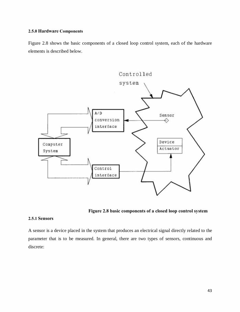
43
2.5.0 Hardware Components
Figure 2.8 shows the basic components of a closed loop control system, each of the hardware
elements is described below.
Figure 2.8 basic components of a closed loop control system 2.5.1 Sensors
A sensor is a device placed in the system that produces an electrical signal directly related to the
parameter that is to be measured. In general, there are two types of sensors, continuous and
discrete:

44
a) Continuous.
. Figure 2.9 an example of a continuous sensor Continuous sensors produce a continuous electrical signal, such as a voltage, current,
conductivity, capacitance, or any other measurable electrical property. For example, sensors of
different kinds can be used to measure temperature, such as thermistors and thermocouples. A
thermocouple will produce a voltage difference that increases as the temperature increases.
Continuous sensors are used where values taken by a state variable are required and an on/off
state is not sufficient, for example, to measure pressure drop across a sand filter.
45
b) Discrete.
Discrete sensors are basically switches, mechanical or electronic, that indicate whether an on or
off condition exists. Discrete sensors are useful for indicating thresholds, such as the opening and
closure of devices (vents, doors, alarms, valves, etc.). They can also be used to determine if a
threshold of an important state variable has been reached. Some examples of discrete sensors are
a float switch to detect if the level in a storage tank is below a minimum desirable level, a
switching tensiometer to detect if soil moisture is above a desired threshold, and a thermostat to
indicate if a certain temperature has been reached. When combined with time, pulses from
switches can be used to measure rates. For example, to the volume of fuel, water or chemical
solution passing through a totalizing flow meter with a magnetically activated switch, or the
speed of a rotating flywheel.
Sensors are an extremely important component of the control loop because they provide the basic
data that drive an automatic control system. Understanding the operating principle of a sensor is
very important. Sensors many times do not react directly to the variable being measured. For
example, when a mercury thermometer is used to measure temperature, temperature is not being
measured, rather, a change in volume due to a change in temperature is measured. Because there
is a unique relationship between the volume and the temperature the instrument can be directly
calibrated to provide temperature readings. The ideal sensor responds only to the "sensed"
variable, without responding to any other change in the environment. It is important to
understand that sensors always have a degree of inaccuracy associated with them and they may
be affected by other parameters besides the "sensed" variable. The classical example is that of
soil moisture measurement using electrical conductivity probes. The electrical signal produced
by this sensor is closely related to soil moisture, but is greatly affected by temperature and
dissolved salts (fertilizers, etc.) in the soil. Another important factor related to the sensor is its
time response. A sensor must deliver a signal that reflects the state of the system within the
frame of time required by the application. Using the soil moisture measurement example, the
sensor must be able to "keep up" with the changes in soil moisture that are caused by
evapotranspiration. Thus, proper selection of the sensors and understanding the principle of
operation is critical to the success of a control system. Some of the variables that are often
measured in computer based control systems are the following:
46
1) Flow rate, 2) pressure, 3) soil-moisture, 4) air temperature, 5) wind speed, 6) solar radiation,
7) relative humidity, 8) total salts in irrigation water, and 9) pH of irrigation water.
2.5.2 A/D interface
Since computer systems work internally with numbers (digits), the electrical signals resulting
from the sensors must be converted to digital data. This is done through specialized hardware
referred to as the Analog-to-Digital (A/D) interface. Discrete signals resulting from switch
closures and threshold measurements are converted to 0 and 1. Continuous electrical (analog)
signals produced by the sensors signals are converted to a number related to the level of the
sensed variable. The accuracy of the conversion is affected by the resolution of the conversion
equipment. In general, the higher the resolution the better the accuracy. For, example if a
pressure sensor produces a voltage signal ranging from 0 to 5 volts for a range of pressure of 10
atmospheres, an 8 bit resolution A/D board will be able to detect a change in voltage of about
5/255 volts which will results in measurable increments of 10/255 atmospheres. If the resolution
of the A/D board was 12 bit, the board would be able to detect a change in voltage of about
5/4095 volts or a measurable increment of 10/4095 atmospheres.
2.5.3 Computer system
The A/D conversion hardware is directly connected to the computer system. Given the current
state of technology, the computer system may be a PC (personal computer), a minicomputer, or a
specially designed machine that is solely dedicated to the control task. The type of machine
depends on the type of application, and is greatly affected by factors such as environment
characteristics, complexity of the controlled system, and the speed with which conversions need
to take place (controlling a high speed extruder requires much more speed than a golf-course
irrigation system). Many agricultural applications can be economically carried out using personal
computers (PC), as is evident by the increasing number of system integrators and equipment
manufactures that are marketing PC-based control systems. Also, many manufacturers of control
equipment have designed and manufactured specialized computer control systems.

47
2.5.4 Control Interface:
Using control software, decisions may be made to modify the controlled system. The actual
changes are achieved by having devices within the system that will affect the controlled
variables. These devices are controlled through actuators that respond to signals from the control
interface. The devices may be of the nearly continuous or discrete types. For example, the
extension of a robot arm of a citrus harvesting robot requires the use of a continuous signal from
the computer, while a fan or a valve requires only an on/off (discrete) signal from the computer.
In general, any device that can be powered electrically can be computer controlled.
2.6 Computer-based Controller Topologies
2.6.1 Centralized computer
The simplest form in which a computer control system can be arranged is to use a single
computer system that included the necessary support hardware and software to support data
acquisition and control. The basic system describe in Figure 2.10 is this type of system.
2.6.2 Satellite systems
A centralized computer can be linked to other devices that have specialized purposes. One such
type of device can be a datalogging system (a computer in itself) used to collect weather data.
Also, in large complex systems, a central computer can be used to download instruction to
intelligent controllers.

48
Figure 2.10 Example of computer based topologies
Communications between the central control computer can be implemented in a variety of ways:
a) Serial or parallel communication links.
b) Telephone link using serial communications.
c) Carrier wave using powerline modulation.
d) Communications bus.
Telephone and serial links can be hardwired or wireless. Figure 2.10 shows the components of a
typical high-end commercially available computer based control system.
2.7 Controllers
2.7.0 Electromechanical Controllers
Electromechanical controllers use an electrically driven clock and mechanical switching (gear
arrays) to activate the irrigation stations. These types of controllers are generally very reliable
and not too sensitive to the quality of the power available. They generally are not affected by
spikes in the power, and unless surges and brownouts are of such magnitude that they will
damage the motor, they will continue to operate. Even if there is a power outage, the
programmed schedule will not be lost and is generally delayed only for the duration of the power

49
outage. However, because of the mechanically-based components they are limited in the features
they provide. Figure 2.11 shows the components of a commercially available electromechanical
controller.
Figure 2.11 a typical commercially available electromechanical controller. 2.7.1 Electronic Controllers
Electronic controllers rely on solid state and Integrated circuits to provide the clock/timer,
memory and control functions. These types of systems are more sensitive to powerline quality
than electromechanical controllers and may be affected by spikes, surges and brownouts.
Particularly spikes and surges are common in rural areas in Florida where lightning tends to be
frequent and intense. These types of systems may require electrical suppression devices in order
to operate reliably. Because of the inherent flexibility of electronic devices, these controllers tend
to be very flexible and provide a large number of features at a relatively low cost. Figure 2.12
shows the components of a commercially available electronic controller (irrigation timer).
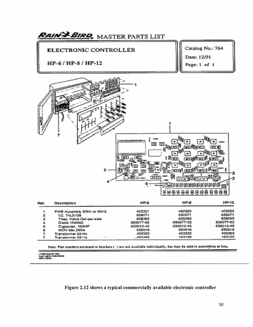
50
Figure 2.12 shows a typical commercially available electronic controller
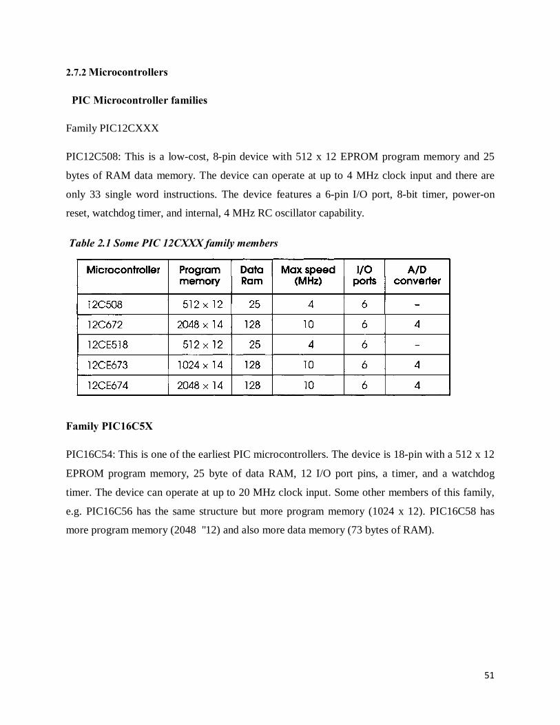
51
2.7.2 Microcontrollers
PIC Microcontroller families
Family PIC12CXXX
PIC12C508: This is a low-cost, 8-pin device with 512 x 12 EPROM program memory and 25
bytes of RAM data memory. The device can operate at up to 4 MHz clock input and there are
only 33 single word instructions. The device features a 6-pin I/O port, 8-bit timer, power-on
reset, watchdog timer, and internal, 4 MHz RC oscillator capability.
Table 2.1 Some PIC 12CXXX family members
Family PIC16C5X
PIC16C54: This is one of the earliest PIC microcontrollers. The device is 18-pin with a 512 x 12
EPROM program memory, 25 byte of data RAM, 12 I/O port pins, a timer, and a watchdog
timer. The device can operate at up to 20 MHz clock input. Some other members of this family,
e.g. PIC16C56 has the same structure but more program memory (1024 x 12). PIC16C58 has
more program memory (2048 • 12) and also more data memory (73 bytes of RAM).

52
Table 2.2 Some PIC16C5X family members
Family PIC16CXXX
PIC16C554: This microcontroller has similar architecture to the PIC16C54 but the instructions
are 14-bits wide. The program memory is EPROM with 512 x 14 and the data memory is 80
bytes of RAM. There are 13 I/O port pins, a timer, and a watchdog timer.
Some other members of this family, e.g. PIC16C71 incorporates four channels of A/D converter,
1024 x 14 EPROM program memory, 36 bytes of data RAM, timer, and watchdog timer.
PIC16F877 is a sophisticated microcontroller which offers eight channels of A/D converters,
8192 x 14 program memory, 368 bytes of data memory, 33 I/O port pins, USART, I2C bus
interface, SPI bus interface, 3 timers, and a watchdog timer. PIC16F84 is a very popular
microcontroller, offering 1024 x 14 flash EEPROM program memory, 68 bytes of data RAM, 64
bytes of EEPROM data memory, 13 I/O port pins, timer, and a watchdog timer.

53
Table 2.3 Some PIC16CXXX and PIC16FXXX family members
Family PIC17CXXX and PIC18CXXX
PIC17C42: This microcontroller has a 2048 x 16 program memory. The data memory is 232
bytes. In addition, there are 33 I/O port pins, USART, 4 timers, a watchdog timer, 2 data capture
registers, and PWM outputs. PIC 17C44 is similar but offers more program memory.
PIC18CXXX members of this family include PIC18C242 type microcontroller with 8192 x 16
program memory, 512 bytes of data memory, 23 I/O port pins, 5 A/D channels (10-bits wide),
USART, I2C, and SPI bus interfaces, PWM outputs, 4 timers, watchdog timer, compare and
capture registers, and multiply instructions.
All memory of the PIC microcontroller family is internal and it is usually not very easy to
expand the memory externally. No special hardware or software features are provided for
expanding either the program memory or the data memory. The program memory is usually
sufficient for small dedicated projects. However the data memory is generally small and may not
be enough for medium to large projects unless a bigger and more expensive member of the

54
family is chosen. For some large projects even this may not be enough and the designer may
have to choose a microcontroller from a different manufacturer with a larger data memory, or a
microcontroller where the data memory can easily be expanded (e.g. the Intel 8051 series).
Table 2.4 Some PIC17CXXX and PIC18CXXX family members
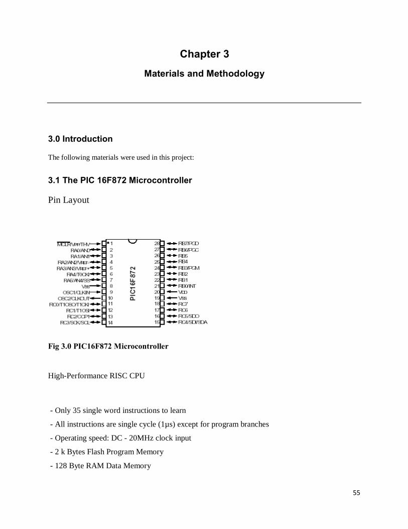
55
Chapter 3
Materials and Methodology
3.0 Introduction
The following materials were used in this project:
3.1 The PIC 16F872 Microcontroller
Pin Layout
Fig 3.0 PIC16F872 Microcontroller
High-Performance RISC CPU
- Only 35 single word instructions to learn
- All instructions are single cycle (1µs) except for program branches
- Operating speed: DC - 20MHz clock input
- 2 k Bytes Flash Program Memory
- 128 Byte RAM Data Memory

56
- 64 Byte EEPROM Data Memory
- In-circuit serial programming
- Interrupt Capability (up to 10 sources)
Peripheral Features
- High current sink/source: 25mA
- Two 8-bit timer/counter(TMR0,TMR2) with 8-bit programmable prescalar
- One 16 bit timer/counter(TMR1)
- One Capture, Compare, PWM module
- 10-bit, 5-channel Analog-to-Digital converter
- Synchronous Serial Port (SSP) with SPI (Master mode) and I2C (Master/Slave)
- Watchdog Timer (WDT) with separate RC oscillator
Special Microcontroller Features
- Power-On Reset
- Power-up Timer (PWRT) and Oscillator Start-Up Timer (OST)
- Power saving SLEEP mode
- Programmable code protection
- Selectable Oscillator Options
CMOS Technology
- Low power, high speed CMOS FLASH technology
- Fully Static Design
- Low Power Consumption
- < 2mA @ 5V, 4MHz

57
- 20µA typical @ 3V, 32kHz
- < 1µA typical standby current
I/O and Packages
- 22 I/O pins with individual direction control
- 28-pin DIP
3.2 CM 3 Pyranometer,
The CM3 pyranometer(Kipp and Zonen, Delft Holland) is an instrument for measuring the solar
irradiance. The sensor construction is such that it measures the solar energy that is received from
the whole hemisphere (180o field of view). The output is expressed in Watts per mitre square.
List of specifications
- Response time 95% 18s
- Zero offsets 1 and 2
- 1: 200 W/m2 thermal radiation < 15W/m2
- 2:5 K/h change in ambient
- Temperature <4W/m2
- Non-stability <1% change per year
- Non-linearity ±2.5% (D1000W/m2)
- Directional error for beam radiation < ±25W/m2 at 1000 W/m2
- Spectral selectivity ±5% (350-1500nm)
- Temperature dependence of sensitivity 6% (-10 to +40oC)

58
3.3 System physical design
Context Diagram
Fig 3.1 Irrigation System’s physical design
The system consists of a radiation sensor called the CM3 Pyranometer, which coverts radiation into a voltage and a signal amplification circuit. The analogue voltage signal is then fed into the Analogue to Digital Converter in the PIC Microcontroller. The PIC microcontroller is the one that controls the relay, depending on the inputs from the CM3 Pyranometer. All the data displays are made on the LCD display.
CM3 Pyranometer
Signal amplification
Relay
LCD
PIC microcontroller
Irrigation valve and pump

59
3.4 Data acquisition
The data acquisition process consists of getting radiation readings from the CM3 Pyranometer into then PIC Microcontoller. An electronic circuit is required for signal amplification or signal de-amplification, depending on the nature of the voltage produced by the input device. It is also required for powering the devices, for display purposes and control purposes. Below are the parts of the electronic circuit designed for the irrigation control:
3.4.0 Electronic Circuit diagram design
Components of the Electronic Circuit
1) Power supply unit
Fig 3.2 Irrigation systems power supply unit

60
The power supply consists of a transformer to step down the voltage from the mains to 5 volts. It also consists of a regulator which makes sure that the voltage supply remains constant at 5 volts regardless of the load present. The diode is there to make sure that the current flows in one direction, this result in current flowing in pulses, therefore the capacitors are there for smoothing the current.
2) 2-digit Seven segment display
Fig 3.3 Irrigation system’s display unit
The 2 digit display consists of the 2 digit LCDs with a capacity of displaying 1 digit at a time. In order to display two digits, we have to multiplex. The multiplexing involves the use of transistors which are controlled by sending either bit 1 or 0 to the pin 0 of Port C. If we send a 1, the current
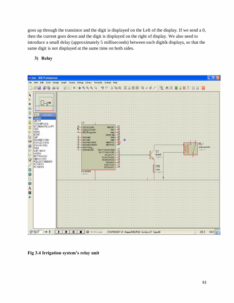
61
goes up through the transistor and the digit is displayed on the Left of the display. If we send a 0, then the current goes down and the digit is displayed on the right of display. We also need to introduce a small delay (approximately 5 milliseconds) between each digit’s displays, so that the same digit is not displayed at the same time on both sides.
3) Relay
Fig 3.4 Irrigation system’s relay unit

62
The relay consists of a transistor and an adapter connected to the mains. To turn on the relay, we need to send bit 1 though pin 5 of Port C, and to turn off we need to clear the bit.
Physical circuit design
Fig 3.3 Irrigation system’s electronic circuit
Every component of the circuit is connected to the PIC Microcontroller. The ports have to be
configured as input or output ports in the TRIS registers. The input devices are connected to port
A, the display is connected on Port B, and the relay is connected on Port C. The power supply
powers the devices on the circuit including the microcontroller. The inputs are generated by

63
varying the readings on the CM3 Pyranometer. The reading is proportional to the voltage that is
produced by the CM3 Pyranometer. Inside the PIC Microcontoller there’s an Analogue to digital
converter that converts analogue readings to digital values. After the completion of the Analogue
to digital conversion, the digital value will be stored in the lower part of the ADRES register,
which is called the ADRESL.
3.5 Data Processing and Irrigation sequencing
Algorithm Design
While (sub-season a)
start :
read radiation every 15 minutes
Rs = Current reading
Rs-1 = Previous reading
integrate between aRs and aRs-1 over 15 minutes or
alternatively find area under the graph, assuming a smooth increase
Total water lost = ∑ water lost in all 15 min intervals
determine(water to be applied or replaced today)
determine(time to irrigate)
start irrigation()
induce an independent delay(time to irrigate)
End irigation()
End

64
While (sub-season b)
start :
read radiation every 15 minutes
Rs = Current reading
Rs-1 = Previous reading
integrate between aRs and aRs-1 over 15 minutes or
alternatively find area under the graph, assuming a smooth increase
Total water lost = ∑ water lost in all 15 min intervals
determine(water to be applied or replaced today)
determine(time to irrigate)
start irrigation()
induce an independent delay(time to irrigate)
End irigation()
End
While (sub-season c,d,e,………………)
start :
read radiation every 15 minutes
Rs = Current reading
Rs-1 = Previous reading

65
integrate between aRs and aRs-1 over 15 minutes or
alternatively find area under the graph, assuming a smooth increase
Total water lost = ∑ water lost in all 15 min intervals
determine(water to be applied or replaced today)
determine(time to irrigate)
start irrigation()
induce an independent delay(time to irrigate)
End irigation()
End
The Data processing consists of getting the digital value from the ADRESL register every 15
minutes. Then we have to integrate between the previous readings over the entire 15 minute
interval. The totals over each interval are stored in the general purpose registers. Then we have
to calculate the total over the entire day. The totals for the entire day and the entire day are stored
over multiple registers. We then have to divide the totals by the irrigation application rate to find
the time that we need to irrigate.

66
Chapter 4
Conclusions, recommendations and future work
4.0 Conclusions
In this thesis, we have evaluated the acquisition and processing of data using an 8-bit register. Our results
show that using an 8 bit of the acquisition of data whose magnitude can range from 0-1400 watts/m2
introduces a great deal of inaccuracy in terms of data processing because for the data to be fed into the
PIC Microcontroller a transformation( a divide by 10 transformation) has to be performed on the data.
Further, during division, we had problems in storing fractions, and therefore another transformation (a
multiply by 20 transformation) had to be performed also. So during the whole process several
transformations had to be performed on the data so that the data remains in a usable state. The storage of
values was also a problem since in some instances a single value had to be stored over multiply register
and making arithmetic operations using such values become tedious and therefore confusing for the
programmer.
Further the instruction set was too small so much that most of the basic functions which are readily
available in most instruction sets, like division, multiplication, square root, etcetera had to be
reconstructed from first principles, whilst other complex functions like integration proved to be extremely
difficult to construct. However we managed to find close substitutes to these functions, but it also
introduced a great deal of inaccuracy.
The PIC Microcontroller 16F872 is not time conscious like the computer and other more advanced
controllers, so several independent delays had to be introduced especially for day keeping and during
irrigation. The introduction of long independent delays using 8 bit time was very difficult, considering
the total available storage space that was available. Hence this resulted in independent delays having
some a great deal of dependence, especially in very long independent delays.

67
4.1 Recommendations
In situations where accuracy in terms of data processing is a priority we will need to introduce a
slightly more powerful processor in terms of working memory, storage memory, and also with a
slightly bigger instructions with well constructed basic functions e.g 16 bit processor. We will
also need to embed some more flexible language like C or C++ within the assembly language
code so as to make it easier to construct complex functions.
4.2 Future work
This research did not look at how to deal with power cuts, although it is easy to back-up the power for the
electronic circuit, the irrigation pump and equipment requires a lot of electricity. We will need to
incorporate into the electronic circuit a sub-circuit which can detect the presence of electricity from the
main after a shut down. The signal can then be used to resume or start irrigation after the shutdown.
Artificial intelligence would also be required for this kind of work.

68
REFERENCES
[1] Bates LM, Hall AE. 1981. Stomatal closure with soil water depletion not associated with changes in bulk leaf water status. Oecologia 50, 62–65.
[2] Journal of Experimental Botany, Vol. 55, No. 407, Water-Saving Agriculture Special Issue, pp. 2427–2436, November 2004 doi:10.1093/jxb/erh213 Advance Access publication 30 July, 2004
[3] Irrigation scheduling: advantages and pitfalls of plant-based methods Hamlyn G. Jones* Plant Research Unit, Division of Environmental and Applied Biology, School of Life Sciences, University of Dundee at SCRI, Invergowrie, Dundee DD2 5DA, UK Received 12 November 2003; Accepted 27 May 2004
[4] Bates LM, Hall AE. 1981. Stomatal closure with soil water depletion not associated with changes in bulk leaf water status. Oecologia 50, 62–65.
[5] Stocker O. 1956. Die Abha¨ngigkeit des transpiration von den unweltfaktoren. In: Ruhland W, ed. Encyclopedia of plant physiology, Vol. 3. Berlin: Springer-Verlag.
[6] Tardieu F, Simonneau T. 1998. Variability among species of stomatal control under fluctuating soil water status and evaporative demand: modelling isohydric and anisohydric behaviours. Journal of Experimental Botany 49, 419–432.
[7] Schultz HR. 2003. Differences in hydraulic architecture account for near-isohydric and anisohydric behaviour of two field-grown Vitis vinifera L. cultivars during drought. Plant, Cell and Environment 26, 1393–1405.
[8] Hsiao T. 1973. Plant responses to water stress. Annual Review of Plant Physiology 24, 519–570.
[9] Huguet J-G, Li SH, Lorendeau JY, Pellous G. 1992. Specific micromorphometric reactions of fruit trees to water stress and irrigation scheduling automation. Journal of Horticultural Science 67, 631–40.
[10] Massacci A, Jones HG. 1990. Use of simultaneous analysis of gasexchange and chlorophyll fluorescence quenching for analysingthe effects of water stress on photosynthesis in apple leaves. Trees: Structure and Function 4, 1–8.
[11] Davies WJ, Zhang J. 1991. Root signals and the regulation of growth and development of plants in drying soil. Annual Review of Plant Physiology and Molecular Biology 42, 55–76.

69
[12] Moriana A, Fereres E. 2002. Plant indicators for scheduling irrigation of young olive trees. Irrigation Science 21, 83–90.
[13] Franks PJ, Cowan IR, Farquhar GD. 1997. The apparent feedforward response of stomata to air vapour pressure deficit: information revealed by different experimental procedures with two rainforest trees. Plant, Cell and Environment 20, 142–145.
[14] Fereres E, Goldhamer DA. 2003. Suitability of stem diameter variations and water potential as indicators for irrigation scheduling of almond trees. Journal of Horticultural Science and Biotechnology 78, 139–144.
[15] Slatyer RO. 1967. Plant water relationships. London and New York: Academic Press.
[16] Barrs HD. 1968. Determination of water deficits in plant tissues. In: Kozlowski TT, ed. Water deficits and plant growth, Vol. I. London and New York: Academic Press, 235–368.
[17] Peretz J, Evans RG, Proebsting EL. 1984. Leaf water potentials for management of high frequency irrigation on apples. Transactions of the American Society of Agricultural Engineers 27, 437–442.
[18] McCutchan H, Shackel KA. 1992. Stem water potential as a sensitive indicator of water stress in prune trees (Prunus domestica L. cv. French). Journal of the American Society for Horticultural Research 117, 606–611.
[19] Simonneau T, Habib R. 1991. The use of tree suckers to estimate root water potential. Plant, Cell and Environment 14, 585–591.
[20] Garnier E, Berger A. 1987. The influence of drought on stomatalconductance and water potential of peach trees growing in the field. Scientia Horticulturae 32, 249–263.
[21] Lorenzo-Minguez P, Ceulemans RJM, Gabriels R, Impens I, Verdonck O. 1985. Effect of short-term water stress on leaf gas exchange processes and plant water potential in Schefflera. HortScience 20, 932–934.
[22] Dixon MA, Tyree MT. 1984. A new stem hygrometer, corrected for temperature-gradients and calibrated against the pressure bomb. Plant, Cell and Environment 7, 693–697.
[23] Jones HG. 1973. Estimation of plant water status with the betagauge. Agricultural Meteorology 11, 345–355.
[24] Jones HG. 1983. Estimation of an effective soil water potential at the root surface of transpiring plants. Plant, Cell and Environment 6, 671–674.
[25] McBurney TA. 1992. The relationship between leaf thickness and plant water potential. Journal of Experimental Botany 43, 327–335.
[26] Burquez R. 1987. Leaf thickness and water deficits in plants: a tool for field studies. Journal of Experimental Botany 38, 109–114.

70
[27] Selle´s G, Berger A. 1990. Physiological indicators of plant water status as criteria for irrigation scheduling. Acta Horticulturae 286, 87–100.
[28] Kang SZ, Davies WJ, Shan L, Cai HJ (eds). 2003. Water-saving agriculture and sustainable use of water and land resources. Xian, PR China: Shaanxi Science and Technology Press.
[29] Brough DW, Jones HG, Grace J. 1986. Diurnal changes in the water-content of stems of apple trees as influenced by irrigation. Plant, Cell and Environment 9, 1–7.
[30] Granier A. 1987. Evaluation of transpiration in a Douglas fir stand by means of sap-flow measurements. Tree Physiology 3, 309–319.
[31] Cermak J, Kucera J. 1981. The compensation of natural temperature gradient at the measuring point during sap flow-rate determination in trees. Biologia Plantarum 23, 469–471.
[32] Eastham J, Gray SA. 1998. A preliminary evaluation of the suitability of sap flow sensors for use in scheduling vineyard irrigation. American Journal of Enology and Viticulture 49, 171–176.
[33] Ginestar C, Eastham J, Gray S, Iland P. 1998a. Use of sap-flow sensors to schedule vineyard irrigation. I. Effects of post-veraison water deficits on water relations, vine growth, and yield of Shiraz grapevines. American Journal of Enology and Viticulture 49, 413–420.
[34] Ameglio T, Archer P, Cohen M, Valancogne C, Daudet FA, Dayau S, Cruiziat P. 1998. Significance and limits in the use of predawn leaf water potential for tree irrigation. Plant and Soil 205,155–167.
[35] Giorio P, Giorio G. 2003. Sap flow of several olive trees estimatedwith the heat-pulse technique by continuous monitoring of a singlegauge. Environmental and Experimental Botany 49, 9–20.
[36] Remorini D, Massai R. 2003. Comparison of water status indicators for young peach trees. Irrigation Science 22, 39–46.
[37] Ehret DL, Lau A, Bittman S, LinW, Shelford T. 2001. Automated monitoring of greenhouse crops. Agronomie 21, 403–414.
[38] Wronski EB, Homes JW, Turner NC. 1985. Phase and amplitude relations between transpiration, water potential and stem shrinkage. Plant, Cell and Environment 8, 613–622.
[39] Steudle E. 2001. The cohesion-tension mechanism and the acquisition of water by plant roots. Annual Review of Plant Physiology and Plant Molecular Biology 52, 847–875.
[40] Milburn JA. 1979. Water flow in plants. London: Longmans.
[41] Tyree MT, Dixon MA. 1983. Cavitation events in Thuja occidentalis L.? Ultrasonic emissions from the sapwood can be measured. Plant Physiology 66, 397–405.

71
[42] Tyree MT, Sperry JS. 1989. Vulnerability of xylem to cavitation and embolism. Annual Review of Plant Physiology 40, 19–38.
[43] Sandford AP, Grace J. 1985. The measurement and interpretation of ultrasound from woody stems. Journal of Experimental Botany 36, 298–311.
[44] Yang SF, Qian DP, Huo XJ, Okushima L, Sase S. 2003. Computerized precision irrigation system based on estimation of crop water stress with acoustic emission technique. In: Kang SZ, Davies WJ, Shan L, Cai HJ, eds. Water saving agriculture and sustainable use of water and land resources. Xian, PR China: Shaanxi Science and Technology Press, 480–483.
[45] Raschke K. 1960. Heat transfer between the plant and the environment. Annual Review of Plant Physiology 11, 111–126.
[46] Hipps LE, Ashrar G, Kanemasu ET. 1985. A theoretically-based normalization of the environmental effects on foliage temperature. Agricultural and Forest Meteorology 35, 113–122.
[47] Martin DL,Wehner DJ, Throssell CS. 1994. Models for predicting the lower limit of the canopy-air temperature difference of two cool season grasses. Crop Science 34, 192–198.
[48] Diaz-Espejo A, Verhoef A. 2002. Use of IR thermography for assessing the canopy exchange processes in sunflowers. In: Villalobos FJ, Testi L, eds. Proceedings of VII European Society of Agronomy Congress, Cordoba. European Society of Agronomy, 265–266.
[49] Plant RE, Horrocks RD, Grimes DW, Zelinski LJ. 1992. CALEX/ Cotton: an integrated expert system application for irrigation scheduling. Transactions of the American Society of AgriculturalEngineers 35, 1833–1838.
[50] Evans DE, Sadler EJ, Camp CR, Millen JA. 2001. Spatial canopy temperature measurements using center pivot mounted IRTs. Proceedings of the 5th International Conference on Precision Agriculture, Bloomington, Minnesota, July, 2000, 1–11.
[51] Colaizzi PD, Barnes EM, Clarke TR, Choi CY, Waller PM, Haberland J, Kostrzewski M. 2003. Water stress detection under high frequency sprinkler irrigation with water deficit index. Journal of Irrigation and Drainage Engineering 129, 36–42.
[52] Dogan Ibrahim, Microcontroller based temperature monitoring and control, ISBN: 0750655569,Publisher: Elsevier Science & Technology Books, Pub. Date: September 2002
[53] Myke Predko, PICmicro® Microcontroller Pocket Reference book, Copyright © 2001 by
The McGraw-Hill Companies
[54] Thomas Schmidt, 28-Pin, 8-Bit CMOS FLASH Microcontroller with 10-Bit A/D, 2002, Microchip Technology Incorporated,
[55] Hess, Tim . M., 1996. Evapotranspiration estimates for water balance scheduling in the UK. Irrigation News, 25: 31-36, Silsoe College, Cranfield University, MK45 4DT, UK

72
[56] http://www.ipcc.ch/publications_and_data/ar4/wg3/en/ch3s3-5-2.html
[57] Irrigation scheduling: advantages and pitfalls of plant-based methods
[58] Hamlyn G. Jones* Plant Research Unit, Division of Environmental and Applied Biology, School of Life Sciences, University of Dundee at SCRI, Invergowrie, Dundee DD2 5DA, UK
[59] David Mieklejohn. Programming baseline PIC in C, Gooligam Electronics
[60] www.jxb.oxfordjournals.org

73
Annexes Annex A Initializing the PIC16F870
LIST p=16F870
#include "P16F870.INC"
; Macro to generate a MOVLW instruction that also causes a model break:
break MACRO arg
DW 0x3100 | (arg & H'FF')
ENDM
cblock 0x20
count, lc1,lc2,lc3,k,
day,temp,DIVIDENT,DIVISOR,DIVRES,TEMPY8,TEMPX8,IDX16,RESULT8,TEMPX,
TEMPY, RESULT, MULY , MULP, MULRES,REM,REMS,RESULTS,WLE,IAPR
;
endc
; Vector for normal start up.
org 0
goto start
org 4
goto inthlr
Annex B Look-up table for the analogue to digital conversion
; Analogue voltage to hexadecimal conversion Look up table
HEXTABLE ;clrf PCLATH ; Clear PCLATH for zero page
addwf PCL,F
retlw 0x00 ; 0

74
retlw 0x00
retlw 0x01
retlw 0x00
retlw 0x02
retlw 0x00
retlw 0x03
retlw 0x00
retlw 0x04
retlw 0x00
retlw 0x05
retlw 0x00
retlw 0x06
retlw 0x06
retlw 0x07
retlw 0x07
retlw 0x08
retlw 0x08
retlw 0x09
retlw 0x09
retlw 0x00
retlw 0x0A ;10
retlw 0x00
retlw 0x0B
retlw 0x00
retlw 0x0C
retlw 0x00
retlw 0x0D
retlw 0x00
retlw 0x0E
retlw 0x00
retlw 0x0F
retlw 0x00
retlw 0x10
retlw 0x00
retlw 0x11
retlw 0x00
retlw 0x12
retlw 0x00
retlw 0x13
retlw 0x00
retlw 0x14 ;20
………………………………….
…………………………………..
………………………………..
retlw 0x64 ;100

75
retlw 0x00
retlw 0x65
retlw 0x66
retlw 0x67
retlw 0x00
retlw 0x68
retlw 0x00
retlw 0x69
retlw 0x00
retlw 0x6A
retlw 0x00
retlw 0x6B
retlw 0x00
Annex C
PIC Microcontroller Sub-routines
;division_function
devide MOVF DIVIDENT,W
MOVWF TEMPX8
MOVF DIVISOR,W
MOVWF TEMPY8
CALL DIVV8
MOVF RESULT8,W
MOVWF DIVRES
MOVF DIVISOR,W
MOVWF MULY
MOVF DIVRES,W
MOVWF MULP
CALL MULTIPLY
SUBWF DIVIDENT,W
MOVWF REM
return
DIVV8
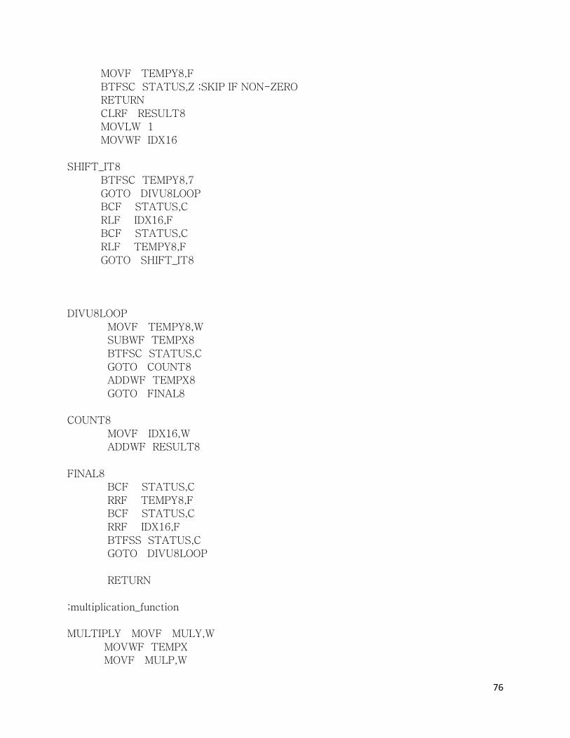
76
MOVF TEMPY8,F
BTFSC STATUS,Z ;SKIP IF NON-ZERO
RETURN
CLRF RESULT8
MOVLW 1
MOVWF IDX16
SHIFT_IT8
BTFSC TEMPY8,7
GOTO DIVU8LOOP
BCF STATUS,C
RLF IDX16,F
BCF STATUS,C
RLF TEMPY8,F
GOTO SHIFT_IT8
DIVU8LOOP
MOVF TEMPY8,W
SUBWF TEMPX8
BTFSC STATUS,C
GOTO COUNT8
ADDWF TEMPX8
GOTO FINAL8
COUNT8
MOVF IDX16,W
ADDWF RESULT8
FINAL8
BCF STATUS,C
RRF TEMPY8,F
BCF STATUS,C
RRF IDX16,F
BTFSS STATUS,C
GOTO DIVU8LOOP
RETURN
;multiplication_function
MULTIPLY MOVF MULY,W
MOVWF TEMPX
MOVF MULP,W

77
MOVWF TEMPY
CALL MULV8
MOVF RESULT,W
MOVWF MULRES
RETURN
MULV8
CLRF RESULT
MULU8LOOP
MOVF TEMPX,W
BTFSC TEMPY,0
ADDWF RESULT
BCF STATUS,C
RRF TEMPY,F
BCF STATUS,C
RLF TEMPX,F
MOVF TEMPY,F
BTFSS STATUS,Z
GOTO MULU8LOOP
RETURN
; Display function for Analogue to Digital conversion values
disp_adc bsf STATUS,RP0 ; Bank 1.
movf ADRESL,W ; Get ADRES into W.
CALL HEXTABLE
return
disp_adc2 bsf STATUS,RP0 ; Bank 1.
bcf STATUS,RP0 ; Bank 0.
movwf PORTB ; Write it to port
bsf PORTC,6 ; Toggle latch enable
nop ; Wait

78
nop ; Wait
bcf PORTC,6 ; Toggle latch enable
movf ADRESL,W ; Get ADRES into W.
movwf PORTB ; Write it to port
bsf PORTC,7 ; Toggle latch enable
nop ; Wait
nop ; Wait
bcf PORTC,7 ; Toggle latch enable
return
Annex D
PIC configurations and control program for the automated irrigation system
; Main program starts here:
start
clrf 0x73
clrf 0x74
clrf 0x75
clrf 0x76
clrf 0x77
clrf 0x78
clrf PORTC
movwf PORTB ; Ensure PORTB is zero before we enable it.
movwf PORTC ; Ensure PORTC is zero before we enable it.
movwf count ; reset count value.
movwf CCPR1H ; Clear.
movwf CCPR1L ; Clear.
; Set up ports:
bsf STATUS,RP0 ; Select Bank 1
movlw 0x01
movwf TMR0
movlw 0xFF ; Set W to mask for all inputs.
movwf TRISA ; set TRISA register as inputs.
movlw 0x00 ; Set W to mask for all inputs.
movwf TRISA ; set TRISA register as inputs.

79
bcf STATUS,RP0 ; Select Bank 1
bsf PORTA,0
bcf PORTA,0
bsf PORTA,0
bcf PORTA,0
bsf STATUS,RP0 ; Select Bank 0
movlw 0xFF ; Set W to mask for all inputs.
movwf TRISA ; set TRISA register as inputs.
clrf TRISB ; Set TRISB register as outputs.
clrf TRISC ; Set TRISC register as outputs.
movlw 0x81 ; ADFM=1, all inputs analogue, +VREF enabled.
movwf ADCON1 ; Save it.
bcf STATUS,RP0 ; Select Bank 0.
movlw 0xC1 ; Clock/Channel select and enable.
movwf ADCON0 ; Save it.
movlw 0x01 ; Number of loops of 255 clocks.
call swait2 ; Wait for acquire time.
start_new_day movlw 0x60
movwf day
;Analogue to digital conversion module
do_conv bsf ADCON0,GO
wait_eoc btfsc ADCON0,GO ; Is bit still set?
goto wait_eoc ; loop and wait for end of conversion.
bcf STATUS,RP0 ; Ensure we have bank 0.
bsf PORTC,0 ; Show ISR in progress results.
incf count,F ; Increment count.
call disp_adc ; read captured value.
movwf 0x25
bcf STATUS,C
addwf 0x26,W ; Adding current and previous value

80
movwf DIVIDENT ; devision to get resultant
movlw 0x02
movwf DIVISOR
CALL devide
movf DIVRES,W
movwf 0x72 ; store result in 0x72
movwf MULY ; multiplication by a constant 3
movlw 0x03
movwf MULP
CALL MULTIPLY
movf MULRES,W
movwf 0x72 ; store result in 0x72
movwf DIVIDENT ; division by a constant 20
movlw 0x14
movwf DIVISOR
CALL devide
movf DIVRES,W
movwf 0x72
movf REM,W
movwf 0x73
movlw 0x04
subwf 0x73,1
btfsc STATUS,C ;test for register overfolow
goto here4 ; if clear, got label here3
btfss STATUS,C ; if not clear goto label here2
goto here5
here4 movlw 0x05 ; if remainder is 5 or more
addwf 0x72,1 ; then add a constant 5 to the result
goto here6
here5 movlw 0x04 ; if remainder is less than 5
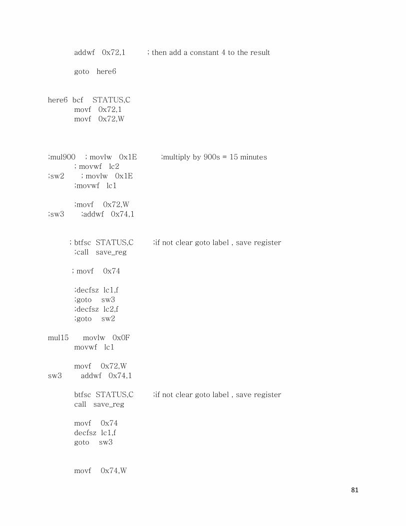
81
addwf 0x72,1 ; then add a constant 4 to the result
goto here6
here6 bcf STATUS,C
movf 0x72,1
movf 0x72,W
;mul900 ; movlw 0x1E ;multiply by 900s = 15 minutes
; movwf lc2
;sw2 ; movlw 0x1E
;movwf lc1
;movf 0x72,W
;sw3 ;addwf 0x74,1
; btfsc STATUS,C ;if not clear goto label , save register
;call save_reg
; movf 0x74
;decfsz lc1,f
;goto sw3
;decfsz lc2,f
;goto sw2
mul15 movlw 0x0F
movwf lc1
movf 0x72,W
sw3 addwf 0x74,1
btfsc STATUS,C ;if not clear goto label , save register
call save_reg
movf 0x74
decfsz lc1,f
goto sw3
movf 0x74,W

82
addwf 0x75,1
movf 0x75,1
btfsc STATUS,C ;if not clear goto label , save register
call save_reg
movf 0x27,W
call disp_adc2
movf 0x25 ,W
movwf 0x26
;Routine to LIGHT LCD to show that the system is reading a value
LightLCD1 movlw 0x13
movwf PORTC
CALL swait
;CALL swait
;CALL swait
;CALL swait
;CALL swait
;CALL swait
;CALL swait
;CALL swait
CLRF PORTC
bcf PORTC,0 ; Remove progprogress results bit.
movlw 0x40 ; Count
movwf count ; Save it.
loop1 nop ; Dilly...
nop ; Dally...
nop ; Dilly...
decfsz count ; Decrement loop counter
goto loop1 ; Loop if no zero.
decfsz day

83
goto do_conv ; Do another conversion.


