
Modeling Land Use Change in Chittenden County, VT
Austin Troy, PhD, [email protected] Voigt, graduate research assistant, [email protected]
University of VermontRubenstein School of Environment and Natural Resources
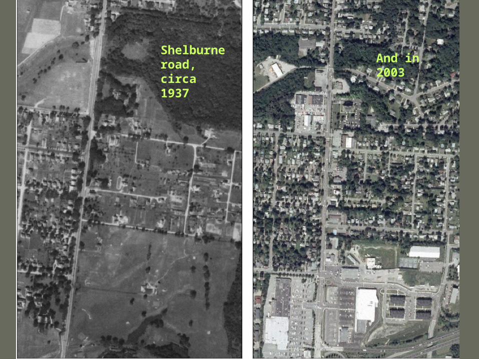
Shelburne road, circa 1937
And in 2003

New North End and Colchester, 1937
New North End and Colchester in 2003

Dorset St.Spear St.
So. Burlington, 1937

So. Burlington, 2003
Dorset St.
Spear St.

198720021987
Some areas of major new development between 87 and 02

Close up: Shelburne development since 1950
Click for animation

Chittenden County Land Use1982 – 1997
1982
Misc2%
Crops9%
Forest59%
Water14%
Pasture9%
Developed7%
1997
Misc1%
Crops7%
Forest60%
Developed12%
Pasture6%
Water14%
YEAR
1930
Min = 0.79 per / mi2
Max = 3712 per / mi2
YEAR
1940
Min = 0.79 per / mi2
Max = 4221 per / mi2
YEAR
1950
Min = 0.59 per / mi2
Max = 4709 per / mi2
YEAR
1960
Min = 0.00 per / mi2
Max = 5189 per / mi2
YEAR
1970
Min = 1.98 per / mi2
Max = 5111 per / mi2
YEAR
1980
Min = 1.78 per / mi2
Max = 4418 per / mi2
YEAR
1990
Min = 0.40 per / mi2
Max = 4650 per / mi2
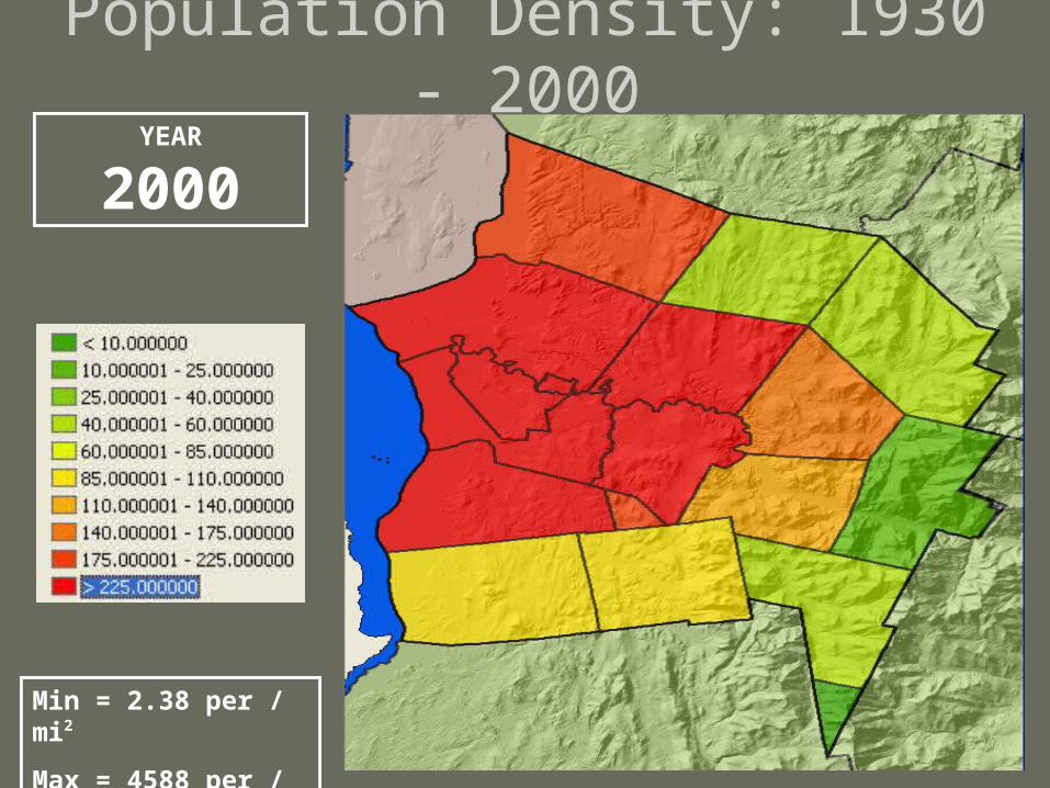
YEAR
2000
Min = 2.38 per / mi2
Max = 4588 per / mi2
Population Density: 1930 - 2000

Percent Occupied
Household Demographics1990 2000
Median Household IncomeAverage Age of Head of HouseholdAverage Household Size

Project: “Dynamic land use and transportation modeling”
• Purpose: to simulate future land use and environmental impact in Chittenden County under baseline and alternative scenarios
• Tools: UrbanSim and TransCAD + original modules for simulating environmental impact
• US DOT FHWA funded; 2006-2008• Research started in 2003 under EPA grant• Conducted at UVM Spatial Analysis Lab• Collaborators: Resource Systems Group (RSG,
Inc), CCRPC, CCMPO, UVM (Breck Bowden, Jon Erickson, Dave Capen, others)
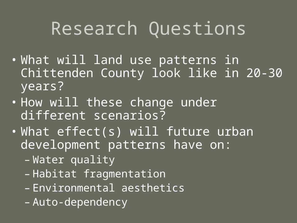
Research Questions
• What will land use patterns in Chittenden County look like in 20-30 years?
• How will these change under different scenarios?
• What effect(s) will future urban development patterns have on:– Water quality– Habitat fragmentation– Environmental aesthetics– Auto-dependency

Scenario Modeling with UrbanSim
• Simulate impacts of user-defined scenarios– Highway infrastructure– Utility infrastructure– Zoning– Land use policies (e.g., growth centers)– Exogeneous shocks (e.g. energy prices)
• Intended to facilitate discourse not predict policy adoption
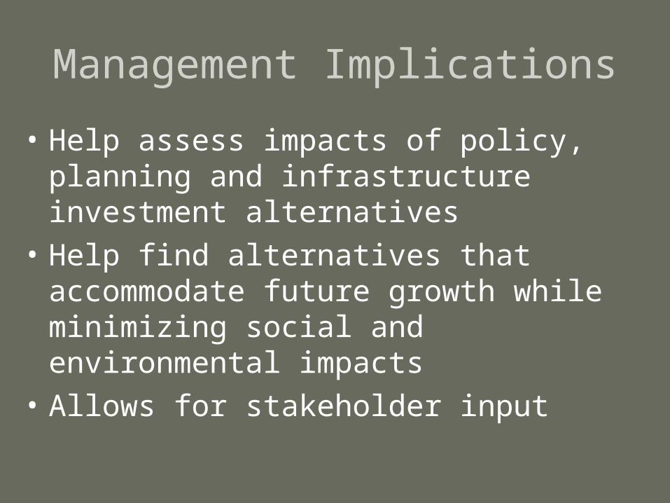
Management Implications
• Help assess impacts of policy, planning and infrastructure investment alternatives
• Help find alternatives that accommodate future growth while minimizing social and environmental impacts
• Allows for stakeholder input
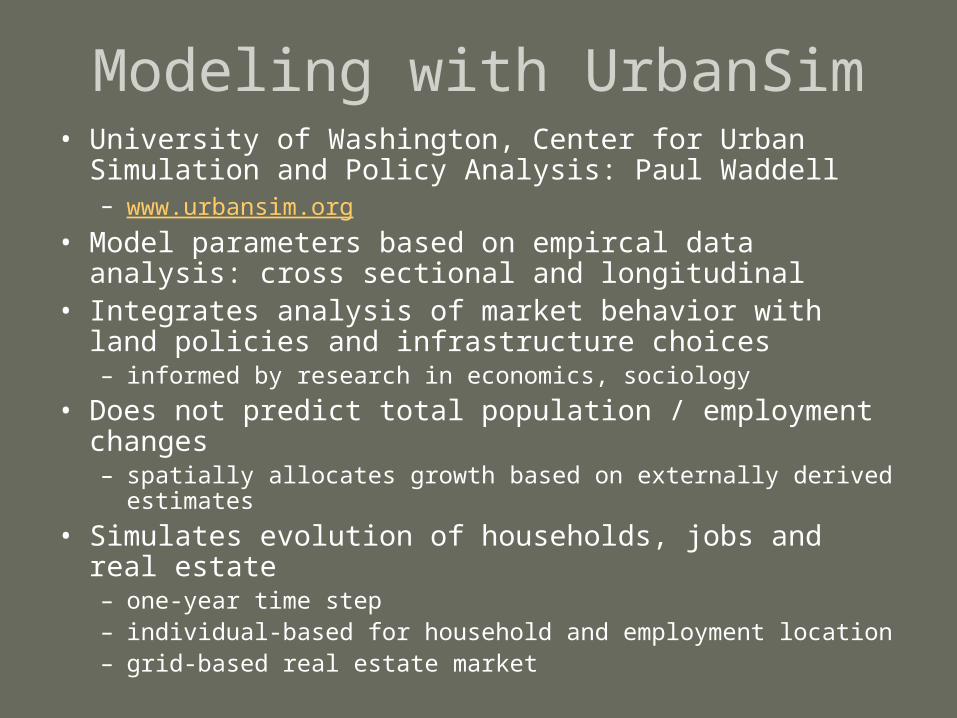
Modeling with UrbanSim• University of Washington, Center for Urban Simulation
and Policy Analysis: Paul Waddell– www.urbansim.org
• Model parameters based on empircal data analysis: cross sectional and longitudinal
• Integrates analysis of market behavior with land policies and infrastructure choices– informed by research in economics, sociology
• Does not predict total population / employment changes– spatially allocates growth based on externally derived estimates
• Simulates evolution of households, jobs and real estate– one-year time step– individual-based for household and employment location– grid-based real estate market
from Waddell, et al, 2003

Dynamic Disequilbrium Approach
• Dynamic: feedback loops between components– Multiple processes interacting: households, jobs, real
estate development and location choices– Different processes work at different time scales
• short: travel behavior• medium: household / business location• long: real estate / infrastructure development
• Disequilibrium: – avoids oversimplification of general equilibrium
conditions (perfectly competitive market, products are homogenous, resources are mobile, present and future costs are known, etc.)
– Does not re-equilibrate sectors at each step
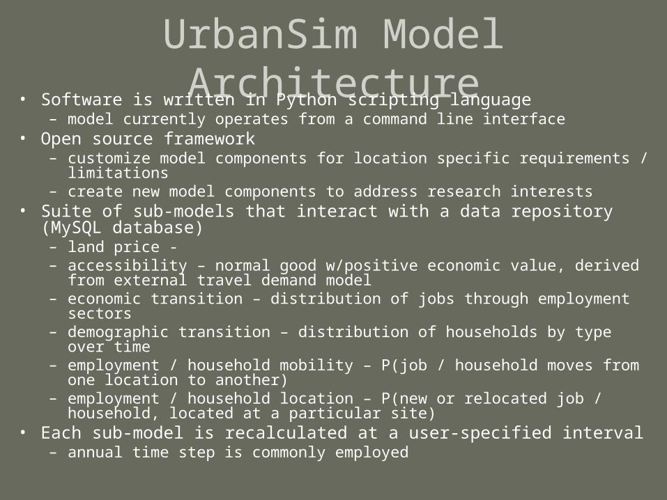
UrbanSim Model Architecture• Software is written in Python scripting language
– model currently operates from a command line interface• Open source framework
– customize model components for location specific requirements / limitations– create new model components to address research interests
• Suite of sub-models that interact with a data repository (MySQL database)– land price - – accessibility – normal good w/positive economic value, derived from external
travel demand model– economic transition – distribution of jobs through employment sectors– demographic transition – distribution of households by type over time– employment / household mobility – P(job / household moves from one location
to another)– employment / household location – P(new or relocated job / household,
located at a particular site)• Each sub-model is recalculated at a user-specified interval
– annual time step is commonly employed
from Waddell, et al, 2003

data store
modeloutput
output visualization
submodels
modified from Waddell et al., 2001
export model
control totals
TDM outputs
macro-economic
model
travel demand model
user specified events
scenario assumptions
model coordinator
UrbanSim Model Architecture

Household Synthesis
• Create synthetic baseline population (Beckman, et al, 1996)– iterative proportional fitting (IPF) algorithm that creates a household
distribution that matches block group marginal distributions
• Data inputs– US Census
• marginal distribution tables (STF-3A) at the block group level– # households, total population, income, automobiles, presence of children,
age of head of household, workers
– Public-Use Microdata Sample (PUMS) 5% sample• detailed description of household characteristics from Public-Use Micro
Area (PUMA)
• Synthetic households assigned to available housing stock

Household Synthesis
Block Group: 500070011002
Grid_ID:23674
HSHLD_ID: 23
AGE_OF_HEAD: 42
INCOME: $65,000
Workers: 1
KIDS: 3
CARS: 4

Travel Demand Model• Often coupled with land use models
– strong interdependence b/t phenomena– relationship widely recognized by research and
government (US DOT: ISTEA 1991, TEA-21 1997)
• Evaluating land use and transportation scenarios– infrastructure performance– investment alternatives– air quality impacts

Travel Demand Model Process Steps
• Area of interest is divided into Traffic Analysis Zones (TAZs)– 340+ in Chittenden Co.
• Four-step process– trip generation: quantify
incoming & outgoing travel by zone
– trip distribution: assign trips to zones
– modal split: estimates trips by mode for each zone
– traffic assignment: identifies trip route
I = 375
O = 216
I = 17
O = 240
Zone ID Walk Bus Drive
17 6 3 27
18 19 14 26
…
340 0 2 126

Accessibility Model
• Consumers value access– work, shopping, recreation– household demographics determine preferences
• Distribution of opportunities weighted by composite utility of all modes of travel to set of opportunities
• Summarize the accessibility from each TAZ to various activities considered relevant for household or business locations
• Assign accessibility values for each gridcell based on TAZ results
• Travel utility remains constant, but the distribution of activities changes annually

Transition Models• Computes changes to previous year employment /
demographic conditions• Models are analogous for employment and
demographic transitions• Use externally derived control totals that specify
growth or decline from previous year totals– employment: distribution of jobs by sector– households: distribution of households by type– control totals define new distributions, or model assumes
static distributions for duration of model run• Probability a specific job / household is lost is
proportional to the spatial distribution of the jobs by sector / household by type

Transition Model Process Steps
• Model process steps– calculate the number of
jobs / households to be added or removed
– in the case of growth• new jobs / households are
added to a list of unplaced jobs / households
– in the case of decline• random subset of jobs /
households removed from set of current jobs / households
• selected job / household locations are marked as vacant
Employment Location Choice
Model
63236
63235
63234
Job ID
Unplaced Jobs
-226532000
1026551999
…
-523901994
3523951993
223601991
23581990
Employment Change
Total Employment
Year
Employment Control Totals
-226532000
1026551999
…
-523901994
3523951993
223601991
23581990
Employment Change
Total Employment
Year
Employment Control Totals
VV

Mobility Models
• Predicts the probability that a particular job / household will move from their current location
• Based on annual mobility rate calculated from prior year observations– employment: transitional change reflecting layoffs,
relocations, closures– households: differential mobility rates for renters,
owners, and households at different life stages• Model structure is analogous for households and
employment• Probability a job / household will move is
proportional to their spatial distribution

Mobility Model Process Steps
• Procedure generates a random number for each job / household
• Compares random number to the job sector / household type mobility rate
• A random number greater than the mobility rate indicates a decision to move– previously occupied locations
added to set of vacant locations– job / household added to set of
unplaced jobs / households
0.21
0.70
0.85
0.79
0.12
0.44
0.010.98
0.86
0.270.89
0.630.52
0.90
0.77
0.82
0.47
mobility rate = 0.83
0.21
0.70
0.85
0.79
0.12
0.44
0.010.98
0.86
0.270.89
0.630.52
0.90
0.77
0.82
0.47
VV
VV V
Unplaced Households
Household Location Choice
Model
2136
1946
1249
…
6677
8600
1599
308
Household ID
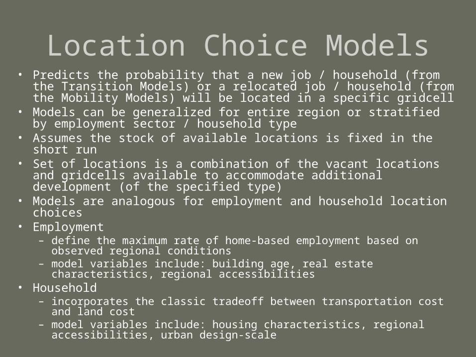
Location Choice Models• Predicts the probability that a new job / household (from the Transition
Models) or a relocated job / household (from the Mobility Models) will be located in a specific gridcell
• Models can be generalized for entire region or stratified by employment sector / household type
• Assumes the stock of available locations is fixed in the short run• Set of locations is a combination of the vacant locations and gridcells
available to accommodate additional development (of the specified type)• Models are analogous for employment and household location choices • Employment
– define the maximum rate of home-based employment based on observed regional conditions
– model variables include: building age, real estate characteristics, regional accessibilities
• Household– incorporates the classic tradeoff between transportation cost and land cost– model variables include: housing characteristics, regional accessibilities,
urban design-scale

Location Choice Model Process Steps
• Processes each job / household in the mover queue in random order
• Queries gridcells for alternative locations to consider
• Selects a location from the list of alternatives
• Selected space becomes unavailable to the remaining jobs / households in the queue
• Placed jobs / households are removed from the list of unplaced jobs / households
• Newly occupied locations are removed from the list of vacancies
Unplaced Households
Household Location Choice
Model
2136
1946
1249
…
6677
8600
1599
308
Household ID

Real Estate Development Model
• Simulates the construction of new development or the intensification of existing development
• Development types: gridcells are classified by the number of residential units and the amount of nonresidential square feet they contain
• Predicts future development patterns based on analysis of prior development events– year built data is key
• Development constraints are based on user-specified decision rules– identify allowable uses within specified development types– identify allowable transitions from one development type to another
• Model variables include: site characteristics, urban design-scale, regional accessibilities, and market conditions
DEV_TYPE_ID NAME MIN_UNITS MAX_UNITS MIN_SQFT MAX_SQFT
1 R1 1 1 0 500
2 R2 2 4 0 999
3 R3 5 9 0 999
4 R4 10 14 0 2499
5 R5 15 21 0 2499
6 R6 22 30 0 2449
7 R7 31 75 0 4999
8 R8 76 1000 0 4999
9 M1 1 9 500 4999
…
18 C2 0 9 15000 34999
19 C3 0 9 35000 13000000
20 I1 0 5 500 14999
21 I2 0 5 15000 34999
22 I3 0 5 35000 13000000
23 Government 0 9 10000 13000000
24 VacantDevelopable 0 0 0 0
25 Undevelopable 0 0 0 0
• Simulates the construction of new development or the intensification of existing development
• Development types: gridcells are classified by the number of residential units and the amount of nonresidential square feet they contain
• Predicts future development patterns based on analysis of prior development events– year built data is key
• Development constraints are based on user-specified decision rules– identify allowable uses within specified development types– identify allowable transitions from one development type to another
• Model variables include: site characteristics, urban design-scale, regional accessibilities, and market conditions

Real Estate Developer Model Process Steps
• Identify the set of allowable transition types for each gridcell
• Estimate the probability of transition from the existing type to each member of the set of allowable types
• New development type is defined as the outcome of the selection process– this includes the possibility of no change
• Update database to reflect new gridcell development types
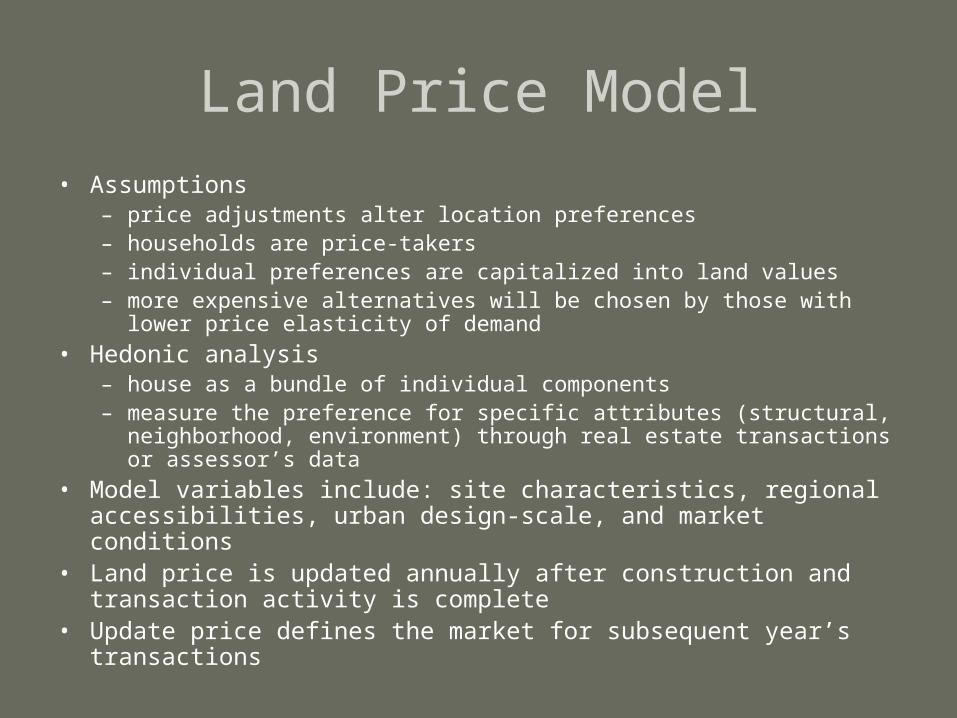
Land Price Model
• Assumptions– price adjustments alter location preferences– households are price-takers– individual preferences are capitalized into land values– more expensive alternatives will be chosen by those with lower price
elasticity of demand
• Hedonic analysis– house as a bundle of individual components – measure the preference for specific attributes (structural, neighborhood,
environment) through real estate transactions or assessor’s data
• Model variables include: site characteristics, regional accessibilities, urban design-scale, and market conditions
• Land price is updated annually after construction and transaction activity is complete
• Update price defines the market for subsequent year’s transactions

UrbanSim and Travel Demand Models
• External to the UrbanSim system
• User-specified time interval for TDM iteration– typical specification is 5 years– processing pattern continues for the duration of
the simulation
TDM accessibilities
Base year database
Model specification
Data prep year 1 year 2 year 3 year 4 year 5
Run submodels
Update database
Run submodels
Update database
Run submodels
Update database
Run submodels
Update database
Run submodels
Update database
Recalculate accessibilities

Model Output• Output database: defines gridcell state at the end of the model run
– data can be cached annually for trouble shooting and further analysis• Indicators
– conveys info on the condition and / or trend of a system attribute– primary mechanism for communicating model results– can be computed at varying levels of aggregation
• TAZ, block group, city, county– examples of predefined indicators
• transportation: per capita gas consumption, % trips walked, % trips SOV• residential development: # units added, density, occupied units, unit value• nonresidential: square feet added, vacancy rate• other: gridcells per development type, area of land converted• households: car ownership, mean income, unplaced households
– system allows user to define new indicators• Data visulatization
– maps– charts– tables
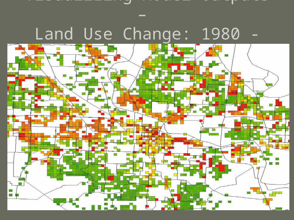
Visualizing Model Outputs – Land Use Change: 1980 - 1994

Vermont UrbanSim Application• Geographic extent
– Chittenden County, VT
• Good site because relatively isolated
• 150 meter grid cells• Annual time step• Model calibration: 1990 –
2002• Model run: 2000 – 2020+• Software: UrbanSim,
TransCAD, MySQL, LimDEP, Access
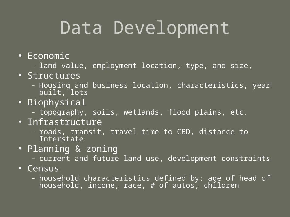
Data Development
• Economic– land value, employment location, type, and size,
• Structures– Housing and business location, characteristics, year built, lots
• Biophysical– topography, soils, wetlands, flood plains, etc.
• Infrastructure– roads, transit, travel time to CBD, distance to Interstate
• Planning & zoning– current and future land use, development constraints
• Census– household characteristics defined by: age of head of household,
income, race, # of autos, children

Control Totals
• Model does not predict population / employment changes– spatially allocates changes to population / employment
• Control totoals are externally derived inputs– population and employment estimates– macroeconomic model of regional economic forecasts– land use and transportation system plans
• Employment: VT Department of Labor• Demographics
– US Census: 1990 & 2000– Public-Use Microdata Samples (5%): 1990 & 2000
• County projections??

Employment Data• 1990 data
– VT Secretary of State database• tradenames & corporations• employment location, description of business
– Greater Burlington Industrial Corporation• inventory of manufacturers w/in Chittenden County
• 2000 data– Claritas business listings
• geocoded location• number of employees / employment sector
• Data conversion– extensive geocoding required for base year data development– # of records = 17981– records placed = 15748 (88%)
• Data attribution– jobs classified by NAICS sector & grouped into general categories– estimate # of employees, square footage / employee, improvement value

Employment DataSECTOR_ID NAME
1 Lumber and wood
2 Other durable
3 Food products
4 Other nondurable
5 Construction
6 Mining
7 Transportation
8 Wholesale trade
9 Retail trade
10 Finance
11 Services
12 Education
13 Government
14 Agriculture
15 Utilities

Employment by Sector: 1970 - 2004
0 10 20 30 40 50 60 70
Construction
Transportation & Utilities
Financial Activities
Education and Health Services
Wholesale / Retail trade
Government total
Manufacturing
Service Providing
Thousands1970 1990 2004

Regional Employment 2000
• Large employers– ~90 businesses with > 75 employees– IBM, IDX, Metro Airlines, Lane Press, UVM
• Small business– ~1100 small businesses with 1 employee– ~4000 small businesses with <= 5 employees
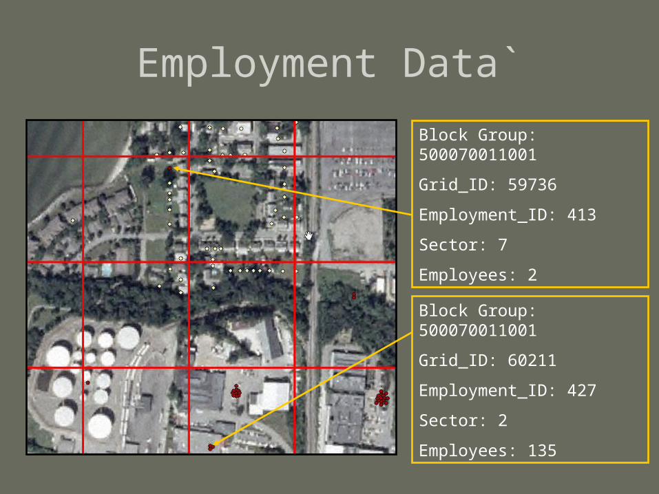
Employment Data`
Block Group: 500070011001
Grid_ID: 60211
Employment_ID: 427
Sector: 2
Employees: 135
Block Group: 500070011001
Grid_ID: 59736
Employment_ID: 413
Sector: 7
Employees: 2

Structure Data• Housing point and parcel data used for
geolocating structures• Sequence of development estimated through
attributing with year built data– Only available digitally for about half of Chittenden
County’s towns (but most of structures)– Other towns had to be modeled with help of e911
database going back to 1998• Property values and some attributes dervied
through new grand list data• Land price model uses VT Dept. of Taxes sales
database to regress sale price against attributes

Year built example
Parcel ID:043000200Year: 1930

Environment sub-modules
• Working on developing sub-modules that take output from UrbanSim to estimate environmental impacts on landscape– Modeling water quality/ watershed
impairment/ nutrient output based on development intensity (Breck Bowden)
– Modeling habitat fragmentation and associated wildlife impacts (David Capen)
– Future project: mobile air quality

Other value added components
• GIS data integration software tools to facilitate the easy visualization of outputs and the manipulation of spatial inputs directly in GIS (Brian Miles)
• Software “wrapper” to more seamlessly integrate UrbanSim and TransCAD (RSG)

Alternative Scenarios: what if?• Policy events
– Change in Act 250– Growth centers legislation– Zoning changes– Urban service boundary
• Investments– New highways– New exits– New utility infrastructure
• Exogenous shift– New major employer– Loss of major employer– Dramatic energy price
increase
base year
establish growth
center(s)policy event 1
employment opportunity
employment event
alter transport
infrastructure
investment
increase density
policy event 2

Scenario modeling allows us to:
• Simulate the effect of these changes on– land use patterns, – densities, – commute times, – energy usage, – mobile emissions, – employment and residential location, – environmental quality
• …And compare them against the baseline

Applications of scenario modeling
• Help towns estimate the effects of planning and zoning changes
• Help the State, RPC, and MPO estimate the impacts of proposed policies with state or regional effects
• Help transportation planners compare transportation project alternatives, including creating a model of induced growth based on Vermont data
• Help stakeholders get involved in the process of decision making

Fall Workshop
• Only a limited number of scenarios can be modeled due to time constraints
• Meeting planned for November 2006 with local, county and state planners to collaboratively define and prioritize a set number of model scenarios
• Please and add your name to the workshop information and availability list during the break or contact us

Lessons so far• Chittenden County is a good site for this model• Data development is difficult and time consuming
– historical data is integral part of model but hard to find– similar data from individual towns often feature
different data formats, attributes, and level of completion
– data requirements for large scale model make application in rural areas challenging
– Data availability limits ability to expand to other counties
• Reward: empirically based model• Stakeholder input and collaboration is key
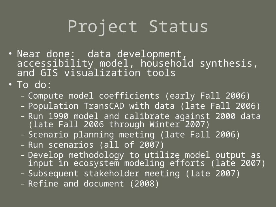
Project Status
• Near done: data development, accessibility model, household synthesis, and GIS visualization tools
• To do:– Compute model coefficients (early Fall 2006)– Population TransCAD with data (late Fall 2006)– Run 1990 model and calibrate against 2000 data (late Fall
2006 through Winter 2007)– Scenario planning meeting (late Fall 2006)– Run scenarios (all of 2007)– Develop methodology to utilize model output as input in
ecosystem modeling efforts (late 2007)– Subsequent stakeholder meeting (late 2007)– Refine and document (2008)

Acknowledgements• Current funder: US DOT Federal Highway
Administration, • Previous funders: US EPA, MacIntire Stennis Program,
Northeastern States Research Cooperative• Graduate researchers past and present: Brian Voigt,
Brian Miles, John D’Agostino, Weiqi Zhou • UVM Collaborators: Breck Bowden, Jon Erickson, David
Capen, Alexei Voinov• UVM Spatial Analysis Lab and Rubenstein School of
Environment• Outside Collaborators:
– RSG: Stephen Lawe and John Lobb– CCRPC: Pam Brangan, Michelle Maresca, Greg Brown– CC MPO: David Roberts– University of Washington Center for Urban Simulation and Policy
Analysis: Paul Waddell, David Socha, many others


