
Misspecification Testing in GARCH-MIDAS Models∗
Christian Conrad† and Melanie Schienle‡
†Heidelberg University, Germany
‡Karlsruhe Institute of Technology, Germany
July 7, 2015
Abstract
We develop a misspecification test for the multiplicative two-component GARCH-
MIDAS model suggested in Engle et al. (2013). In the GARCH-MIDAS model a
short-term unit variance GARCH component fluctuates around a smoothly time-
varying long-term component which is driven by the dynamics of an explanatory
variable. We suggest a Lagrange Multiplier statistic for testing the null hypothesis
that the variable has no explanatory power. Hence, under the null hypothesis the
long-term component is constant and the GARCH-MIDAS reduces to the simple
GARCH model. We derive the asymptotic theory for our test statistic and investi-
gate its finite sample properties by Monte-Carlo simulation. The usefulness of our
procedure is illustrated by an empirical application to S&P 500 return data.
Keywords: Volatility Component Models, LM test, Long-term Volatility.
JEL Classification: C53, C58, E32, G12
∗We would like to thank Richard Baillie, Tilmann Gneiting, Onno Kleen, Karin Loch, Enno Mammen,
Rasmus S. Pedersen, Robert Taylor and Timo Terasvirta for helpful comments and suggestions.†Christian Conrad, Department of Economics, Heidelberg University, Bergheimer Strasse 58, 69115
Heidelberg, Germany, E-Mail: [email protected]; Phone: +49/6221/54/3173.‡Melanie Schienle, Department of Economics (ECON), Karlsruhe Institute of Technology, Schloss-
bezirk 12, 76131 Karlsruhe, Germany, E-Mail: [email protected]; Phone: +49/721/608/47535.

1 Introduction
The financial crisis of 2007/8 has highlighted the need for a better understanding of the
interplay between risks in financial markets and economic conditions. Among others,
Christiansen et al. (2012), Paye (2012) and Conrad and Loch (2014) provide recent evi-
dence for the counter-cyclical behavior of financial volatility.1 In particular, Conrad and
Loch (2014) show that changes in the secular component of stock market volatility can
be anticipated from variables such as the term spread, housing starts or survey expec-
tations on future industrial production. These findings are clearly relevant from a risk
management perspective. Prior to the last financial crisis, risk management exclusively
focused on short-run risks – such as Value at Risk at the one or 10-day horizon – and,
hence, failed to address the risk that risk will change (Engle, 2009). Determining these
long-term risks, however, requires statistical models which allow for effects of changes in
relevant economic variables on the conditional variance of asset returns.
For this reason, an increasing amount of empirical studies has employed the GARCH-
MIDAS framework introduced by Engle et al. (2013) (see, e.g., Asgharian et al., 2013,
Conrad and Loch, 2014, 2015, Dorion, 2013, Opschoor et al., 2014). In a GARCH-MIDAS
specification, the conditional variance consists of two multiplicative components, whereby
economic conditions enter through the smooth long-term component around which a
short-term unit variance GARCH component fluctuates. Besides predictive evidence,
however, it is still an open question whether and which macroeconomic and financial vari-
ables are significant drivers of volatility. This is the case because standard procedures
for misspecification testing in GARCH models do not cover the case of (exogenous) ex-
planatory variables. As most of them also require additive separability of the additional
component under the alternative, their adaption to a general GARCH-MIDAS structure
is not straightforward.2
We develop a misspecification test for the multiplicative two-component GARCH-
MIDAS model. In particular, we propose a Lagrange Multiplier (LM) statistic for testing
the null hypothesis that the long-term component is constant. Thus, under our null
hypothesis, the GARCH-MIDAS model reduces to a simple GARCH. Note that Wald-
type tests like simple t- or F -tests are not straightforward to employ in this context, as
1Their findings complement and extend the earlier work of Officer (1973) and Schwert (1989).2For recent results on properties and estimation of GARCH models with explanatory variables that
enter in an additive fashion see Han and Kristensen (2014) and Han (2015).
2

there exists no asymptotic theory yet for the general case of macroeconomic effects in
the GARCH-MIDAS model. The most recent theoretical results by Wang and Ghysels
(2015) are specific to long-term components that are driven by realized volatility and
only hold in a restrictive parameter space which does not admit our null hypothesis. For
our LM test statistic, we provide a detailed derivation of the asymptotic properties. The
arguments in the derivation rely on the results for the quasi-maximum likelihood estimator
(QMLE) for pure GARCH models in Francq and Zakoıan (2004). The structure of the
proof follows similar lines as the arguments in the proof of Theorem 2 in Halunga and
Orme (2009), who consider general misspecification tests for GARCH models. However,
Halunga and Orme (2009) focus on estimation effects from the correct specification of
the conditional mean and consider additive components only. In our set-up, the volatilty
components are multiplicative, causing substantial differences in the likelihood and test
statistic. For simplicity, we assume that returns have mean zero, thus abstracting from
estimation effects from the mean. In order to derive the asymptotic distribution of the
test statistic, we require the standard assumptions on the GARCH parameters and the
innovation term for the pure GARCH model. In addition, our test needs assumptions
on the moments of the explanatory variable as well as on the observed (return) process.
In a Monte-Carlo simulation, we find good size and power properties in finite samples.
Moreover, we illustrate the usefulness of our procedure by an empirical application to
S&P 500 return data.
Our test statistic is also closely related to the ‘ARCH nested in GARCH’ test for
evaluating GARCH models as proposed by Lundbergh and Terasvirta (2002). While
it is possible to consider their ‘nested ARCH component’ as our long-term component
with a specific choice for the explanatory variable, the specification of their short-term
component is fundamentally different from ours. Under the alternative, in their short-
term component the squared observations are not divided by the long-term component,
which implies that the short-term component is not a GARCH process and, thereby,
leads to a different test indicator. In the Monte-Carlo simulation, we show that even if
we modify their test in order to allow for a general explanatory variable, the difference in
the specification of their short-term component leads to a considerable loss in power in
comparison to our test statistic. The loss in power is the stronger the larger the ARCH
parameter is and the more the long-term component fluctuates.
Finally, our work complements recent research on misspecification testing in mul-
tiplicative component models of the smooth transition type by Amado and Terasvirta
3

(2015), in the Realized GARCH model by Lee and Halunga (2015) and on the estimation
of semiparametric multiplicative component models by Han and Kristensen (2015).
The plan of the paper is as follows. In Section 2, the GARCH-MIDAS model is
introduced and the LM test statistic is derived. This section also contains the main
asymptotic results. Section 3 provides some finite sample evidence in a Monte-Carlo
study. In Section 4, we illustrate how the test can contribute to modeling S&P 500 return
data. Section 5 concludes. All proofs are contained in the Appendix.
2 Model and Test Statistic
In Section 2.1, we first introduce the GARCH-MIDAS specification of Engle et al. (2013)
and then discuss the null hypothesis of our test. We derive the likelihood function and the
test indicator in Section 2.2 and present our main result on the asymptotic distribution
of the test statistic in Section 2.3. Finally, Section 2.4 provides a comparison with the
‘ARCH nested in GARCH’ test.
2.1 The GARCH-MIDAS Model
We define the log-returns as given by
εt = σ0tZt, (1)
where Zt is independent and identically distributed (i.i.d.) with mean zero and variance
equal to one. σ20t is measurable with respect to the information set Ft−1 and denotes the
conditional variance of the returns. We consider the following multiplicative decomposi-
tion of σ20t into a short-term and a long-term component:
σ20t = h∞0t τ 0t (2)
The terminology of decomposing σ20t into a short- and a long-term component follows
Engle et al. (2013). In our setting, the long-term component is the one that is driven
by (exogeneous) explanatory variables and, typically, is smoother than the short-term
component.
The short-term component is specified as a mean-reverting unit variance GARCH(1,1):
h∞0t = (1− α0 − β0) + α0
ε2t−1
τ 0,t−1+ β0h
∞0,t−1 (3)
4
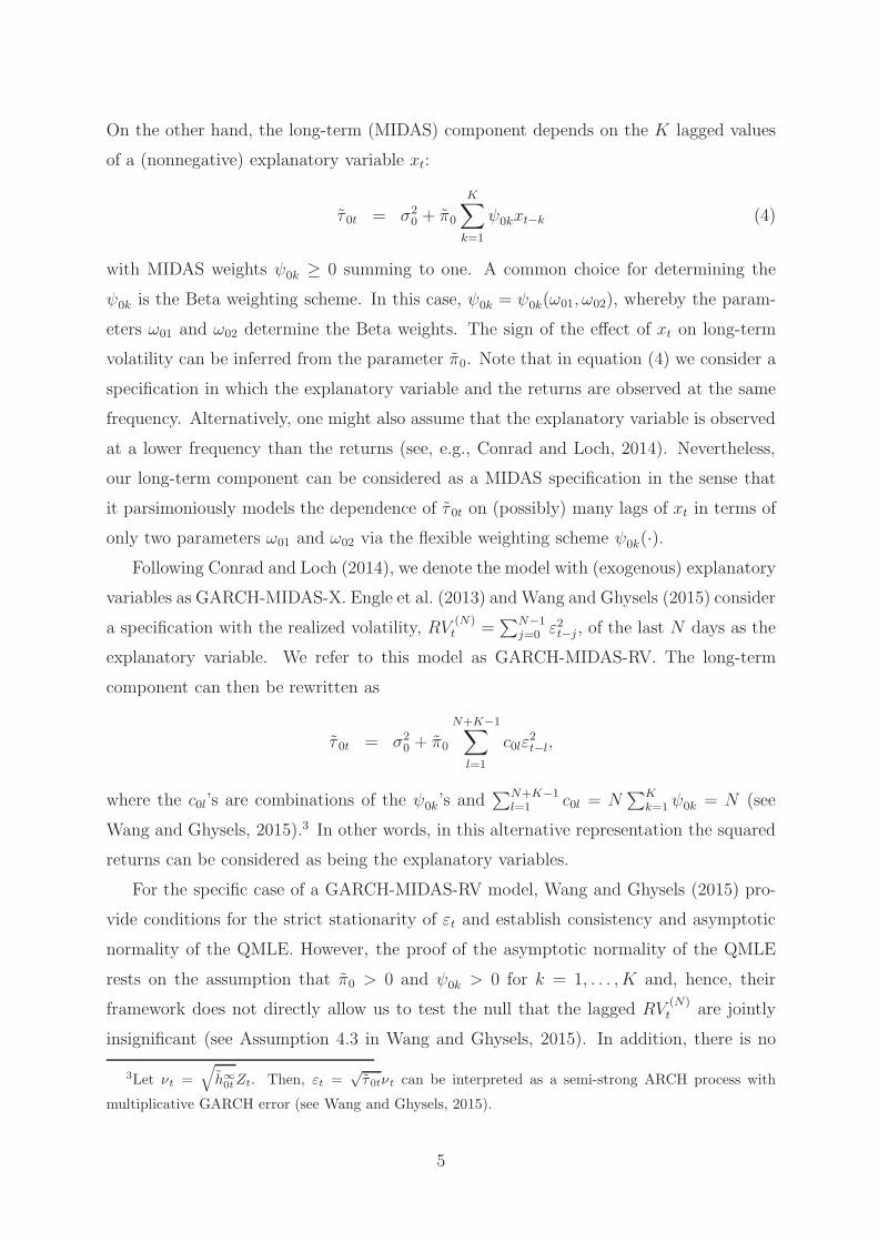
On the other hand, the long-term (MIDAS) component depends on the K lagged values
of a (nonnegative) explanatory variable xt:
τ 0t = σ20 + π0
K∑
k=1
ψ0kxt−k (4)
with MIDAS weights ψ0k ≥ 0 summing to one. A common choice for determining the
ψ0k is the Beta weighting scheme. In this case, ψ0k = ψ0k(ω01, ω02), whereby the param-
eters ω01 and ω02 determine the Beta weights. The sign of the effect of xt on long-term
volatility can be inferred from the parameter π0. Note that in equation (4) we consider a
specification in which the explanatory variable and the returns are observed at the same
frequency. Alternatively, one might also assume that the explanatory variable is observed
at a lower frequency than the returns (see, e.g., Conrad and Loch, 2014). Nevertheless,
our long-term component can be considered as a MIDAS specification in the sense that
it parsimoniously models the dependence of τ 0t on (possibly) many lags of xt in terms of
only two parameters ω01 and ω02 via the flexible weighting scheme ψ0k(·).Following Conrad and Loch (2014), we denote the model with (exogenous) explanatory
variables as GARCH-MIDAS-X. Engle et al. (2013) and Wang and Ghysels (2015) consider
a specification with the realized volatility, RV(N)t =
∑N−1j=0 ε
2t−j , of the last N days as the
explanatory variable. We refer to this model as GARCH-MIDAS-RV. The long-term
component can then be rewritten as
τ 0t = σ20 + π0
N+K−1∑
l=1
c0lε2t−l,
where the c0l’s are combinations of the ψ0k’s and∑N+K−1
l=1 c0l = N∑K
k=1 ψ0k = N (see
Wang and Ghysels, 2015).3 In other words, in this alternative representation the squared
returns can be considered as being the explanatory variables.
For the specific case of a GARCH-MIDAS-RV model, Wang and Ghysels (2015) pro-
vide conditions for the strict stationarity of εt and establish consistency and asymptotic
normality of the QMLE. However, the proof of the asymptotic normality of the QMLE
rests on the assumption that π0 > 0 and ψ0k > 0 for k = 1, . . . , K and, hence, their
framework does not directly allow us to test the null that the lagged RV(N)t are jointly
insignificant (see Assumption 4.3 in Wang and Ghysels, 2015). In addition, there is no
3Let νt =√h∞0tZt. Then, εt =
√τ0tνt can be interpreted as a semi-strong ARCH process with
multiplicative GARCH error (see Wang and Ghysels, 2015).
5

asymptotic theory for the general GARCH-MIDAS-X model yet. We circumvent these
problems by deriving an LM test for the hypothesis that xt does not affect the long-term
component. The LM test requires estimation of the model under the null only. To derive
our test statistic, we re-parameterize equation (2) as follows:
σ20t = h∞0t τ 0t = (σ2
0h∞0t )
(τ 0tσ20
)= h∞0t τ 0t
The short-term component can then be expressed as
h∞0t = ω0 + α0
ε2t−1
τ 0,t−1+ β0h
∞0,t−1 (5)
with ω0 = σ20(1 − α0 − β0) (provided that α0 + β0 < 1). We denote the vector of true
parameters in the short-term component as η0 = (ω0, α0, β0)′. Similarly, the long-term
component can be rewritten as
τ 0t = 1 +K∑
k=1
π0kxt−k = 1 + π′0xt (6)
with π0k = σ−20 π0ψ0k, π0 = (π01, . . . , π0K)
′ and xt = (xt−1, . . . , xt−K)′.
Using this notation, we are interested in testing H0 : π0 = 0 against H1 : π0 6= 0.
Under H0 the long-term component is equal one and the GARCH-MIDAS-X reduces to
the nested GARCH(1,1) with unconditional variance σ20 = ω0/(1 − α0 − β0). Note that
equation (5) is specified such that we can write
h∞0t = ω0 + (α0Z2t−1 + β0)h
∞0,t−1
which means that εt/√τ 0t =
√h∞0tZt follows a GARCH(1,1) both under the null and
under the alternative.
We make the following assumptions about the data generating process under H0.
Assumption 1. η0 ∈ Θ where the parameter space is given by Θ = η = (ω, α, β)′ ∈R
3|0 < ω < ω, 0 < α, 0 < β, α+ β < 1.
Assumption 2. As defined in equation (1), let Zt be i.i.d. with E[Zt] = 0 and E[Z2t ] = 1.
Further, Z2t has a nondegenerate distribution and κZ = E[Z4
t ] <∞.
Assumptions 1 and 2 imply that√h∞0tZt is a covariance-stationary process with uncon-
ditional variance σ20. Further, by Jensen’s inequality, they imply that E[ln(α0Z
2t +β0)] < 0
which ensures that under the null εt is strictly stationary and ergodic (see, e.g., Francq
and Zakoıan, 2004). Finally, the assumption on the existence of a fourth-order moment
of Zt is necessary to ensure that the variance of the score vector exists.
6

2.2 Likelihood Function and Partial Derivatives
We denote the processes that can be constructed from the parameter vectors η = (ω, α, β)′
and π = (π1, . . . , πK)′ given initial observations for εt and xt by ht and τ t. It is im-
portant to distinguish between the observed quasi-likelihood which is based on ht =∑t−1
j=0 βj(ω + αε2t−1−j/τ t−1−j) + βth0 and the unobserved quasi-likelihood function based
on h∞t =∑∞
j=0 βj(ω + αε2t−1−j/τ t−1−j) which depends on the infinite history of all past
observations. The unobserved Gaussian quasi-log-likelihood function can be written as
L∞T (η,π|εT , xT , εT−1, xT−1, . . .) =
T∑
t=1
l∞t (7)
with
l∞t = ln(f(εt|η,π)) = −1
2
[ln(h∞t ) + ln(τ t) +
ε2th∞t τ t
]. (8)
Similarly, conditional on initial values (ε0, h0 = 0,x0) the observed quasi-log-likelihood
can be written as
LT (η,π|εT , xT , εT−1, xT−1, . . . , ε1, x1) =T∑
t=1
lt (9)
with
lt = ln(f(εt|η,π)) = −1
2
[ln(ht) + ln(τ t) +
ε2thtτ t
]. (10)
2.2.1 First derivatives
In the following, we consider the unobserved log-likelihood function. We define the average
score vector evaluated under the null and at the true GARCH parameters as
D∞(η0) =
D∞
η(η0)
D∞π(η0)
=
1
T
T∑
t=1
d∞t (η0) =
1
T
T∑
t=1
d∞
η,t(η0)
d∞π,t(η0)
,
where d∞η,t(η0) = ∂l∞t /∂η
∣∣η0,π=0
and d∞π,t(η0) = ∂l∞t /∂π
∣∣η0,π=0
. Next, we derive explicit
expressions for d∞η,t(η0) and d∞
π,t(η0). First, consider the partial derivative of the log-
likelihood with respect to η:
∂l∞t∂η
=1
2
[ε2t
h∞t τ t− 1
](1
h∞t
∂h∞t∂η
+1
τ t
∂τ t∂η
)(11)
with ∂τ t/∂η = (∂xt/∂η)′π. Under the null hypothesis, the long-term component reduces
to unity and the short term component simplifies to h∞t = h∞t |π=0 = ω + αε2t−1 + βh∞t−1.
7

Note that h∞t corresponds to the standard expression of the conditional variance in a
GARCH(1,1). We then distinguish between
d∞η,t(η) =
∂l∞t∂η
∣∣∣∣π=0
=1
2
[ε2th∞t
− 1
]y∞t (12)
with
y∞t =
1
h∞t
∂h∞t∂η
∣∣∣∣π=0
=1
h∞t
∞∑
i=0
βis∞t−i, (13)
where s∞t = (1, ε2t−1, h∞t−1)
′, and the corresponding quantity which is evaluated at η0:
d∞η,t(η0) =
1
2
[ε2th∞0,t
− 1
]y∞0,t, (14)
with h∞0,t = ω0 + α0ε2t−1 + β0h
∞0,t−1 and y∞
0,t = (h∞0,t)−1∑∞
i=0 βi0s
∞0,t−i.
The partial derivative with respect to π leads to:
∂l∞t∂π
=1
2
[ε2t
h∞t τ t− 1
](1
h∞t
∂h∞t∂π
+1
τ t
∂τ t∂π
), (15)
whereby the partial derivative of h∞t is given by
∂h∞t∂π
= −α∞∑
j=0
βj ε2t−1−j
τ 2t−1−j
∂τ t−1−j
∂π. (16)
Since ∂τ t/∂π = xt + (∂xt/∂π)′π, we have ∂τ t/∂π|π=0 = xt and, hence,
d∞π,t(η) =
∂l∞t∂π
∣∣∣∣π=0
=1
2
[ε2th∞t
− 1
]r∞t (17)
with
r∞t = xt − α1
h∞t
∞∑
j=0
βjε2t−1−jxt−1−j . (18)
Similarly as before, the corresponding expression evaluated at η0 is given by:
d∞π,t(η0) =
1
2
[ε2th∞0,t
− 1
]r∞0,t (19)
with
r∞0,t = xt − α01
h∞0,t
∞∑
j=0
βj0ε
2t−1−jxt−1−j . (20)
In summary, we have
D∞(η0) =1
T
T∑
t=1
d∞t (η0) =
1
2T
T∑
t=1
[ε2th∞0,t
− 1
] y∞
0,t
r∞0,t
. (21)
8

Using that under H0: E[ε2t/h
∞0,t] = E[Z2
t ] = 1, it follows that E[d∞t (η0)|Ft−1] = 0 and
Var[d∞t (η0)] = Ω =
Ωηη Ωηπ
Ωπη Ωππ
=
E[d∞
η,t(η0)d∞η,t(η0)
′] E[d∞η,t(η0)d
∞π,t(η0)
′]
E[d∞π,t(η0)d
∞η,t(η0)
′] E[d∞π,t(η0)d
∞π,t(η0)
′]
=1
4(κZ − 1)
E[y∞
0,t(y∞0,t)
′] E[y∞0,t(r
∞0,t)
′]
E[r∞0,t(y∞0,t)
′] E[r∞0,t(r∞0,t)
′]
. (22)
In the proof of Theorem 1 we will show thatΩ is finite and positive definite. This will allow
us to apply a central limit theorem for martingale difference sequences to 1√T
∑Tt=1 d
∞t (η0).
2.2.2 Second derivatives
In the subsequent analysis we also make use of the following second derivatives:
∂d∞η,t(η)
∂η′ = −1
2
ε2th∞t
y∞t (y∞
t )′ +1
2
[ε2th∞t
− 1
]∂y∞
t
∂η′ (23)
and
∂d∞π,t(η)
∂η′ = −1
2
ε2th∞t
r∞t (y∞t )′ +
1
2
[ε2th∞t
− 1
]∂r∞t∂η′ . (24)
We then define
Jηη = −E
[∂d∞
η,t(η0)
∂η′
]=
1
2E[y∞
0,t(y∞0,t)
′] (25)
and
Jπη = −E
[∂d∞
π,t(η0)
∂η′
]=
1
2E[r∞0,t(y
∞0,t)
′]. (26)
Note that d∞η,t(η0) corresponds to the score of observation t in a standard GARCH(1,1)
model and ∂d∞η,t(η0)/∂η
′ to the respective second derivative. Under Assumptions 1 and 2,
it then directly follows from the results for the pure GARCH model in Francq and Zakoıan
(2004) that Jηη is finite and positive definite. Finally, note that Ωηη = 12(κZ − 1)Jηη and
Ωπη = 12(κZ − 1)Jπη. If Zt is normally distributed, then κZ = 3 and Ωηη = Jηη and
Ωπη = Jπη, respectively.
2.3 The LM Test Statistic
The LM test statistic will be based on the observed quantity Dπ(η) =1T
∑Tt=1 dπ,t(η),
where η is the QMLE of η0 estimated under the null. We derive the asymptotic dis-
tribution of the test statistic in three steps. In the first step, we derive the asymptotic
9

normality of the average score evaluated at η0. We then show that the lower part of the
score evaluated at the QMLE can be related to the average score evaluated at η0 in the
following way:√TD∞
π(η) = [JπηJ
−1ηη
: I]√TD∞(η0) + oP (1) (27)
In the final step it is necessary to show that the observed quantity√TDπ(η) has the same
asymptotic distribution as√TD∞
π(η). The LM statistic follows the usual χ2 distribution.
Since the test statistic will be based on the QMLE of η0, we can rely on the following
result from Francq and Zakoıan (2004). If Assumptions 1 and 2 hold and the model is
estimated under the null, the QMLE of the GARCH(1,1) parameters will be consistent
and asymptotically normal:
√T (η − η0)
d−→ N (0, (κZ − 1)J−1ηη) (28)
In the following theorem, we derive the asymptotic distribution of the average score
evaluated at η0. In order to ensure the finiteness of the covariance matrix of the average
score we assume that xt has a finite fourth moment. Additionally, we assume that the
long-term component is minimal in the sense that no equivalent representation which is
of lower order exists.
Assumption 3. xt ≥ 0 is strictly stationary and ergodic with E[|xt|4] < ∞. There exist
no a1, . . . , aS for the long-term component (6) such that∑K
k=1 π0kxt−k =∑S
s=1 asxt−s with
S < K.
For simplicity, we also assume that the explanatory variable takes nonnegative values
only. This assumption is in line with the GARCH-MIDAS-RV model or the specification
of Lundbergh and Terasvirta (2002) with xt = ε2t/h0t (see Section 2.4). For testing
the GARCH-MIDAS-RV against the simple GARCH model, Assumption 3 requires that
under the null the observed process has a finite eighth moment: E[|εt|8] < ∞. The
corresponding constraints on the parameters of the GARCH(1,1) are provided in Francq
and Zakoıan (2010), equation (2.54). Further, Conrad and Loch (2014) have shown that
nonnegative explanatory variables such as the unemployment rate or disagreement among
forecasters are important predictors of financial volatility. Other potential variables could
be interest rates, the VIX or measures of political uncertainty. However, in order to allow
for variables that take negative values, it is straightforward to extend our results to the
case that the long-term component is given by some general nonnegative function τ 0t =
f(π′0xt). For example, Opschoor et al. (2014) employ the specification τ 0t = exp (π′
0xt)
10

with the Bloomberg Financial Conditions Index as the explanatory variable. In addition,
see Remark 2 below.
Theorem 1. If Assumptions 1-3 hold, then
√TD∞(η0)
d−→ N (0,Ω). (29)
In the proof we use the fact that Ωηη is finite and positive definite which follows from
Theorem 2.2 in Francq and Zakoıan (2004).
Next, we consider the asymptotic distribution of the relevant lower part of the score
vector evaluated at η. As an intermediate step, we show that Jπη can be consistently
estimated by
− 1
T
T∑
t=1
∂d∞π,t(η)
∂η′ ,
where η = η0 + oP (1). The result is presented in Proposition 1 in the Appendix. For
doing so, the following Assumption 4 is required which ensures that Jπη(η) is finite with
a uniform bound for all η ∈ Θ.
Assumption 4. E[|εt|4(1+s)] <∞ for some s > 0.
Note that in general ε2t = h∞0t τ 0tZ2t depends on η0 and π0. Under the null, ε
2t = h∞0,tZ
2t
depends on η0 only. In the proof of Proposition 1 we will use this observation to argue
that E[supη|εt|4(1+s)] = E[|εt|4(1+s)].
Theorem 2. If Assumptions 1-4 hold, then
√TD∞
π(η)
d−→ N (0,Σ), (30)
with
Σ = Ωππ − JπηJ−1ηηΩ′
πη
=1
4(κZ − 1)
(E[r∞0,t(r
∞0,t)
′]− E[r∞0,t(y∞0,t)
′](E[y∞
0,t(y∞0,t)
′])−1
E[y∞0,t(r
∞0,t)
′]). (31)
Note that the covariance matrix Σ in equation (31) takes the same form as in Lund-
bergh and Terasvirta (2002). The actual test statistic will be based on the observed
quantity Dπ(η). The following theorem states the test statistic and its asymptotic dis-
tribution.
11
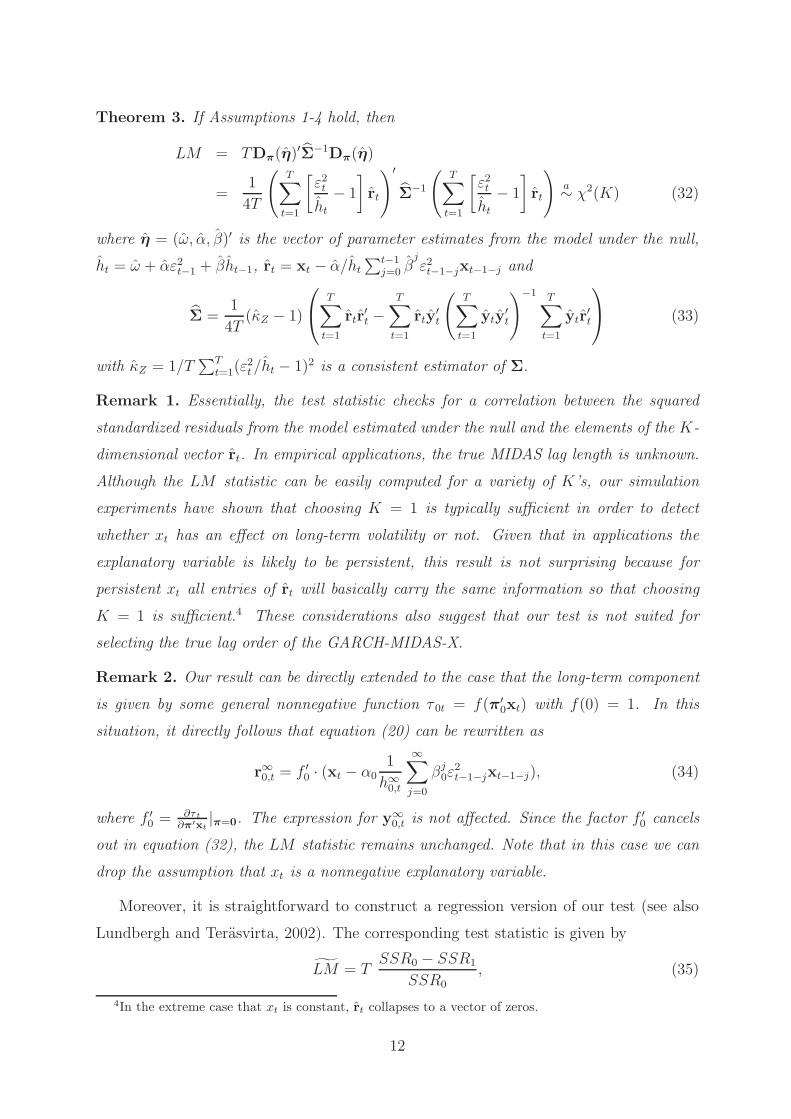
Theorem 3. If Assumptions 1-4 hold, then
LM = TDπ(η)′Σ−1Dπ(η)
=1
4T
(T∑
t=1
[ε2t
ht− 1
]rt
)′
Σ−1
(T∑
t=1
[ε2t
ht− 1
]rt
)a∼ χ2(K) (32)
where η = (ω, α, β)′ is the vector of parameter estimates from the model under the null,
ht = ω + αε2t−1 + βht−1, rt = xt − α/ht∑t−1
j=0 βjε2t−1−jxt−1−j and
Σ =1
4T(κZ − 1)
T∑
t=1
rtr′t −
T∑
t=1
rty′t
(T∑
t=1
yty′t
)−1 T∑
t=1
ytr′t
(33)
with κZ = 1/T∑T
t=1(ε2t/ht − 1)2 is a consistent estimator of Σ.
Remark 1. Essentially, the test statistic checks for a correlation between the squared
standardized residuals from the model estimated under the null and the elements of the K-
dimensional vector rt. In empirical applications, the true MIDAS lag length is unknown.
Although the LM statistic can be easily computed for a variety of K’s, our simulation
experiments have shown that choosing K = 1 is typically sufficient in order to detect
whether xt has an effect on long-term volatility or not. Given that in applications the
explanatory variable is likely to be persistent, this result is not surprising because for
persistent xt all entries of rt will basically carry the same information so that choosing
K = 1 is sufficient.4 These considerations also suggest that our test is not suited for
selecting the true lag order of the GARCH-MIDAS-X.
Remark 2. Our result can be directly extended to the case that the long-term component
is given by some general nonnegative function τ 0t = f(π′0xt) with f(0) = 1. In this
situation, it directly follows that equation (20) can be rewritten as
r∞0,t = f ′0 · (xt − α0
1
h∞0,t
∞∑
j=0
βj0ε
2t−1−jxt−1−j), (34)
where f ′0 = ∂τ t
∂π′xt|π=0. The expression for y∞
0,t is not affected. Since the factor f ′0 cancels
out in equation (32), the LM statistic remains unchanged. Note that in this case we can
drop the assumption that xt is a nonnegative explanatory variable.
Moreover, it is straightforward to construct a regression version of our test (see also
Lundbergh and Terasvirta, 2002). The corresponding test statistic is given by
LM = TSSR0 − SSR1
SSR0
, (35)
4In the extreme case that xt is constant, rt collapses to a vector of zeros.
12
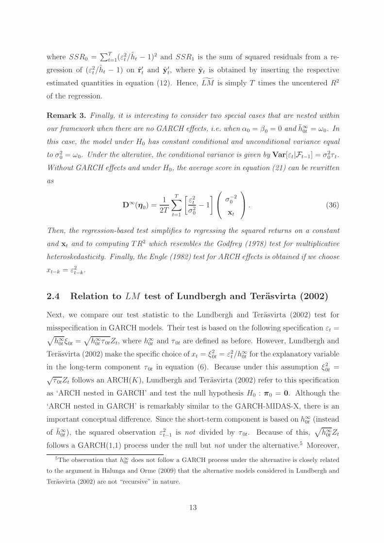
where SSR0 =∑T
t=1(ε2t/ht − 1)2 and SSR1 is the sum of squared residuals from a re-
gression of (ε2t/ht − 1) on r′t and y′t, where yt is obtained by inserting the respective
estimated quantities in equation (12). Hence, LM is simply T times the uncentered R2
of the regression.
Remark 3. Finally, it is interesting to consider two special cases that are nested within
our framework when there are no GARCH effects, i.e. when α0 = β0 = 0 and h∞0t = ω0. In
this case, the model under H0 has constant conditional and unconditional variance equal
to σ20 = ω0. Under the alterative, the conditional variance is given by Var[εt|Ft−1] = σ2
0τ t.
Without GARCH effects and under H0, the average score in equation (21) can be rewritten
as
D∞(η0) =1
2T
T∑
t=1
[ε2tσ20
− 1
] σ−2
0
xt
. (36)
Then, the regression-based test simplifies to regressing the squared returns on a constant
and xt and to computing TR2 which resembles the Godfrey (1978) test for multiplicative
heteroskedasticity. Finally, the Engle (1982) test for ARCH effects is obtained if we choose
xt−k = ε2t−k.
2.4 Relation to LM test of Lundbergh and Terasvirta (2002)
Next, we compare our test statistic to the Lundbergh and Terasvirta (2002) test for
misspecification in GARCH models. Their test is based on the following specification εt =√h∞0t ξ0t =
√h∞0t τ 0tZt, where h
∞0t and τ 0t are defined as before. However, Lundbergh and
Terasvirta (2002) make the specific choice of xt = ξ20t = ε2t/h∞0t for the explanatory variable
in the long-term component τ 0t in equation (6). Because under this assumption ξ20t =√τ 0tZt follows an ARCH(K), Lundbergh and Terasvirta (2002) refer to this specification
as ‘ARCH nested in GARCH’ and test the null hypothesis H0 : π0 = 0. Although the
‘ARCH nested in GARCH’ is remarkably similar to the GARCH-MIDAS-X, there is an
important conceptual difference. Since the short-term component is based on h∞0t (instead
of h∞0t ), the squared observation ε2t−1 is not divided by τ 0t. Because of this,√h∞0tZt
follows a GARCH(1,1) process under the null but not under the alternative.5 Moreover,
5The observation that h∞0t does not follow a GARCH process under the alternative is closely related
to the argument in Halunga and Orme (2009) that the alternative models considered in Lundbergh and
Terasvirta (2002) are not “recursive” in nature.
13

it follows that ∂h∞t /∂π = 0 and, hence, in the Lundbergh and Terasvirta (2002) setting
equation (20) reduces to r∞0,t = (ε2t−1/h∞0,t−1, ε
2t−2/h
∞0,t−2, . . . , ε
2t−K/h
∞0,t−K)
′. Thus, their
LM test statistic is based on [ε2t
ht− 1
]rLTt , (37)
where ht = ω + αε2t−1 + βht−1 and rLTt has entries ε2t−k/ht−k, k = 1, . . . , K. Intuitively,
equation (37) is used to test whether the squared standardized returns are still correlated,
i.e. follow an ARCH process.
In the following section, we will compare the ‘ARCH nested in GARCH’ test of Lund-
bergh and Terasvirta (2002) to our new test in situations in which the true data generating
process (DGP) is a GARCH-MIDAS-X. We implement a regression-based version of the
test as in equation (35) but with rLTt instead of rt. We denote the test statistic by LMLT .
In addition, we consider a modified version of the Lundbergh and Terasvirta (2002) test,
in which we allow for a general regressor xt. In this case, equation (20) is simply given
by r∞0,t = xt = rLT,modt . We denote the corresponding test statistic LMLT,mod. Since
rt − rLT,modt = α/ht
∑t−1j=0 β
jε2t−1−jxt−1−j , our new test, LM , and LMLT,mod can be ex-
pected to perform similarly if, for example, α ≈ 0. On the other hand, we expect that
our test will have better power properties than the modified Lundbergh and Terasvirta
(2002) test when the ARCH effect is strong. Moreover, the expression for rt − rLT,modt
suggests that the difference in power between our new test and the modified Lundbergh
and Terasvirta (2002) test should be stronger in situations in which xt (and, hence, the
long-term component) is more volatile.6
3 Simulation
In this section, we examine the finite sample behavior of the proposed test in a Monte-
Carlo experiment. We simulate return series with T = 1000 observations and use M =
1000 Monte-Carlo replications. The innovation Zt is assumed to be either standard nor-
mally distributed or (standardized) t-distributed with seven degrees of freedom.
6Amado and Terasvirta (2015) discuss testing the null of no remaining ARCH effects in multiplicative
time-varying GARCH models. Our test is closely related to the model they discuss in Section 4.4 of their
paper. However, they provide no asymptotic theory for the test with exogenous explanatory variables.
14
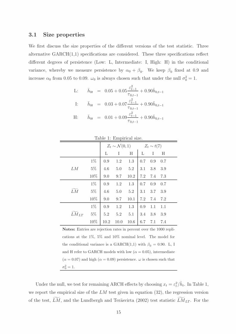
3.1 Size properties
We first discuss the size properties of the different versions of the test statistic. Three
alternative GARCH(1,1) specifications are considered. These three specifications reflect
different degrees of persistence (Low: L, Intermediate: I, High: H) in the conditional
variance, whereby we measure persistence by α0 + β0. We keep β0 fixed at 0.9 and
increase α0 from 0.05 to 0.09. ω0 is always chosen such that under the null σ20 = 1.
L: h0t = 0.05 + 0.05ε2t−1
τ 0,t−1+ 0.90h0,t−1
I: h0t = 0.03 + 0.07ε2t−1
τ 0,t−1+ 0.90h0,t−1
H: h0t = 0.01 + 0.09ε2t−1
τ 0,t−1+ 0.90h0,t−1
Table 1: Empirical size.
Zt ∼ N (0, 1) Zt ∼ t(7)
L I H L I H
1% 0.9 1.2 1.3 0.7 0.9 0.7
LM 5% 4.6 5.0 5.2 3.1 3.8 3.9
10% 9.0 9.7 10.2 7.2 7.4 7.3
1% 0.9 1.2 1.3 0.7 0.9 0.7
LM 5% 4.6 5.0 5.2 3.1 3.7 3.9
10% 9.0 9.7 10.1 7.2 7.4 7.2
1% 0.9 1.2 1.3 0.9 1.1 1.1
LMLT 5% 5.2 5.2 5.1 3.4 3.8 3.9
10% 10.2 10.0 10.6 6.7 7.1 7.4
Notes: Entries are rejection rates in percent over the 1000 repli-
cations at the 1%, 5% and 10% nominal level. The model for
the conditional variance is a GARCH(1,1) with β0 = 0.90. L, I
and H refer to GARCH models with low (α = 0.05), intermediate
(α = 0.07) and high (α = 0.09) persistence. ω is chosen such that
σ20 = 1.
Under the null, we test for remaining ARCH effects by choosing xt = ε2t/ht. In Table 1,
we report the empirical size of the LM test given in equation (32), the regression version
of the test, LM , and the Lundbergh and Terasvirta (2002) test statistic LMLT . For the
15

three test statistics we have to choose the dimension of rt and rLTt , respectively. We opt for
a dimension of one, which implies that the model under the alternative has an ‘ARCH(1)’
long-term component.7 As Table 1 shows, the empirical size of all three versions of the
test statistic is very close to the nominal size when Zt is normally distributed. In case
of Student-t distributed errors, the three test statistics are slightly undersized. For the
LMLT test statistic, this is an observation also made in Lundbergh and Terasvirta (2002)
and Halunga and Orme (2009).
3.2 Power properties
In order to consider a realistic example under the alternative, we base the long-term com-
ponent on actual data. As an explanatory variable, we use the squared daily VIX index,
V IXt, for the period October 2010 to October 2014.8 In addition, we construct monthly
and quarterly rolling window versions of the squared VIX as V IX(N)t = 1
N
∑N−1j=0 V IXt−j,
with N = 22 and N = 65. Figure 1 shows the evolution of the VIX and its rolling window
versions over the sample period. The spikes in the third quarter of 2011 correspond to
the financial turmoil during the European sovereign debt crisis.
0
1
2
3
4
5
6
7
IV I II III IV I II III IV I II III IV I II III
2011 2012 2013 2014
VIX
VIXROLLING22
VIXROLLING65
Figure 1: The figure shows the evolution of V IXt (blue), V IX(22)t (red) and V IX
(65)t
(green) for the period October 2010 to October 2014. The three variables are presented
in daily units.
7The results presented below are robust with respect to increasing the dimension of rt and rLTt . The
corresponding tables are available upon request.8More specifically, we define V IXt as 1/365 times the squared VIX index so that the squared annu-
alized observations are transformed to daily units. The sample is chosen such that T = 1000.
16

The long-term component is given by τ 0t = 1 + 0.5∑K
k=1 ψ0k(ω01, ω02)xt−k, whereby
we specify the MIDAS weights via the following Beta weighting scheme:9
ψ0k(ω01, ω02) =(k/(K + 1))ω01−1 · (1− k/(K + 1))ω02−1
∑Kj=1 (j/(K + 1))ω01−1 · (1− j/(K + 1))ω02−1
. (38)
Table 2 presents the results of the Monte-Carlo simulations. The LM and the LM test
statistics are based on rt with xt ∈ V IXt, V IX(22)t , V IX
(65)t . We present size-adjusted
rejection rates for two versions of the Lundbergh and Terasvirta (2002) test. The modified
Lundbergh and Terasvirta (2002) test, LMLT,mod, is based on rLT,modt but uses the same
xt as in LM and LM . As before, LMLT is based on rLTt with xt = ε2t/ht and, hence, tests
for ‘ARCH nested in GARCH’. In all four test statistics we choose K = 1. We denote
the true MIDAS lag length in the data generating processes under the alternative by K⋆.
We simulate processes with K⋆ ∈ 1, 5, 22. Thus, the results for size-adjusted power in
Table 2 illustrate the performance of the test statistics when K is correctly chosen but
also when K < K⋆.
We first consider the squared VIX as the explanatory variable, i.e. we choose xt =
V IXt. The parameters in the Beta weighting scheme are given by ω01 = 1 and ω02 = 10.
These values ensure that the ψ0k decay monotonically from the first lag. In the GARCH
equation we employ models with α0 = 0.09 (high persistence) and α0 = 0.07 (intermediate
persistence). Besides the size-adjusted power for different values of K⋆, we also report the
following variance ratio: V R = Var(ln(τ 0t))/Var(ln(τ 0th0t)), which reflects the fraction
of the variance of the log conditional variance that is due to the variance of the log
long-term component.10 For example, for K⋆ = 1 and α0 = 0.09, 12.4% of the total
conditional variance is due to the long-term component. When α0 is decreased to 0.07,
the V R increases to 29.5%. Intuitively, decreasing α0, means reducing the variability with
which the short-term component fluctuates around τ 0t.
First, consider the case where α0 = 0.09. For K⋆ = 1, the LM and the LM tests reject
the null hypothesis in 57.2% of the simulations at the nominal 5% level. In contrast, the
rejection rate of the modified Lundbergh and Terasvirta (2002) test, LMLT,mod, is 34.8%
only. When K⋆ is increased to 5 and 22, the long-term component is based on a weighted
average of the values of the VIX during the last week or month. That is, the long-term
9For a detailed discussion of the Beta weighting scheme see Ghysels et al. (2006).10This variance ratio has been employed in Conrad and Loch (2014) as a measure for the relevance of
the long-term component. For example, using the realized volatility as an explanatory variable, they find
a V R of roughly 13% for data on the S&P 500 for the period 1973 to 2010.
17

Table 2: Empirical size-adjusted power for long-term components based on the VIX.
xt V IXt V IX(22)t V IX
(65)t
ω01 = 1, ω02 = 10
α0 = 0.09 α0 = 0.07 α0 = 0.09
K⋆ 1 5 22 1 5 22 1 1
1% 34.8 33.1 21.1 44.7 42.7 29.9 14.3 9.9
LM 5% 57.2 54.8 39.2 66.5 64.6 51.5 36.1 26.5
10% 66.4 64.8 50.7 75.6 74.2 63.0 47.2 35.4
1% 34.8 33.0 21.3 44.5 42.7 29.9 14.4 10.1
LM 5% 57.2 54.7 39.0 66.6 64.6 51.7 36.1 26.6
10% 66.4 64.8 50.8 75.6 74.2 62.9 47.1 35.6
1% 16.0 15.9 13.0 32.6 32.0 27.1 6.6 4.7
LMLT,mod 5% 34.8 34.1 30.3 59.2 58.1 51.1 18.9 15.4
10% 44.2 43.3 38.6 71.1 70.0 65.6 27.1 23.8
1% 0.9 0.9 0.9 1.0 1.0 0.9 0.9 0.8
LMLT 5% 5.9 5.9 5.4 5.6 5.6 5.3 4.8 4.6
10% 10.3 10.5 10.3 10.5 10.7 10.8 9.5 9.4
V R 12.4 12.3 12.1 29.5 29.4 29.0 12.0 10.5
Notes: The table reports the size-adjusted power. The specification of the long term
component is given by τ0,t = 1 + 0.5∑K
k=1 ψ0k(ω01, ω02)xt−k with Beta weighting
scheme (see equation (38)). The GARCH parameters are β0 = 0.9 and ω0 = 1−α0−β0. Innovations Zt are standard normal distributed. K⋆ denotes the true MIDAS lag
length in the DGP. All test statistics are based on K = 1.
component becomes less variable and, hence, more difficult to detect. Consequently, the
power of all three tests deteriorates. Although, the LM and the LM test still have
considerably higher power than LMLT,mod, the difference in power is decreasing when the
long-term component gets smoother. Next, when α0 is decreased to 0.07, this increases
the power of the three tests. For example, for K⋆ = 1 the size-adjusted power at the
nominal 5% level is 66.5% for the LM test. Clearly, with lower α0 and thus less volatile
GARCH component, the long-term component can be detected more easily. As before,
increasing K⋆, i.e. increasing the smoothness of the long-term component, reduces the
power of the tests. In line with the arguments at the end of Section 2.4, the difference
in the power of the LM and LMLT,mod statistics is less strong when α0 is decreased to
18

0.07. Again, the difference in power is the larger the smoother the long-term component
(i.e. the smaller K⋆) is. Finally, the last two columns of Table 2 show the rejection rates
for the case that the long-term component is based on the monthly and quarterly rolling
window versions of the squared VIX. Then, even forK⋆ = 1 the long-term components are
very smooth and the lowest V R’s are observed.11 As expected, the size-adjusted powers
are the lowest for these two cases. Note that in all eight scenarios the original version of
the Lundbergh and Terasvirta (2002) test, LMLT , has no power to detect deviation from
the null.
We performed the same analysis as in Table 2 for the case of Student-t distributed
innovations Zt (see Table 5 in the Appendix). As the table shows, for each specification the
t distributed innovations decrease the V R in comparison to the one that we obtained for
normally distributed innovations. The lower V R’s then lead to a loss of power, i.e. under t
distributed innovations the long-term component is more difficult to detect. However, all
qualitative results regarding the different versions of the test statistics remain unchanged.
We also performed simulations in which we increased K such that it approaches the true
lag length, say K⋆ = 5 or K⋆ = 22. As discussed in Remark 1, given the smoothness of
our explanatory variable, this did not lead to gains in power relative to simply choosing
K = 1.12
In Table 3, we investigate the effects of changing the weighting scheme, ψ0k, on the
power of the test statistics. In the first two columns the weighting scheme is given by
ω01 = 1 and ω02 = 5, i.e. the weights are still monotonically decreasing, but more slowly
than before. This implies that the long-term component becomes less volatile and, hence,
the power of the tests decreases (compare columns one and two of Table 3 with columns
two and three of Table 2). In columns three and four of Table 3 the parameters ω01 and ω02
are chosen such that the weighting schemes are hump-shaped. For example, comparing
column one with column three of Table 3 suggests that for the same lag length K⋆ = 5,
replacing a monotonically decaying weighting scheme with a hump-shaped one decreases
the power of all versions of the test. Again, for all specifications the size-adjusted power
of the LM test is higher than the one of LMLT,mod.
11Note that the model based on the V IX(N)t with lag length K⋆ = 1 can be thought of as representing
a long-term component based on the V IXt as the explanatory variable but with K⋆ = N and weights
equal to 1/N . Thus, by ‘selecting’ an appropriate explanatory variable one can always ensure that K = 1
is sufficient in the test.12The first order autocorrelation of V IXt is 0.95.
19

Table 3: Empirical size-adjusted power for different weighting schemes.
xt = V IXt α0 = 0.09
ω01 = 1, ω02 = 5 ω01 = 3, ω02 = 5 ω01 = 3, ω02 = 20
K⋆ 5 22 5 22
1% 28.2 13.8 19.8 16.7
LM 5% 49.2 29.9 38.6 33.8
10% 60.6 39.8 50.2 45.2
1% 28.2 13.7 19.7 16.7
LM 5% 49.2 29.9 38.7 34.0
10% 60.6 39.9 50.2 45.2
1% 15.0 10.8 12.7 11.7
LMLT,mod 5% 32.8 27.4 30.0 28.6
10% 41.7 35.8 38.5 36.8
1% 0.9 0.9 0.9 0.9
LMLT 5% 5.8 5.3 5.2 5.3
10% 10.5 10.0 10.4 10.4
V R 12.2 11.9 12.2 12.1
Notes: See Table 2.
In summary, the size-adjusted power of the newly proposed test, LM , is higher the
more volatile the long-term component is and the less volatile the short-term component
fluctuates around the long-term component (i.e. the lower α0 is).
4 Empirical Application
Finally, we apply our test and estimate a GARCH-MIDAS-X model for daily log-returns
on the S&P 500 for the period January 2000 to October 2014. As explanatory variables,
we employ the squared VIX, realized volatility as well as the ADS Business Conditions
Index (see Aruoba et al., 2009).13 As before, we construct monthly rolling window ver-
sions of all three variables denoted by V IX(22)t , RV
(22)t and ADS
(22)t . Since ADS
(22)t can
take positive as well as negative values, we specify a ‘log-version’ of equation (4) for the
13Dorion (2013) shows that a GARCH-MIDAS model based on the ADS Business Conditions Index is
informative for the valuation of options.
20

long-term component with ln(τ 0t) = σ20 + π0
∑Kk=1 ψ0kxt−k.
14 We estimate the GARCH-
MIDAS-X models using a restricted Beta weighting scheme (i.e. we impose ω01 = 1 in
equation (38)) and select a MIDAS lag length of 252 (i.e. one year of lagged observa-
tions). Table 4, Panel A, shows the estimates of the parameters of interest for the three
GARCH-MIDAS-X models. First, note that for all three cases the ARCH/GARCH pa-
rameter estimates are basically the same. The estimates of π are positive for the V IX(22)t
and RV(22)t , but negative for the ADS
(22)t . That is, higher expected/realized volatility
leads to an increase in long-term volatility, while an improvement in business conditions
reduces long-term volatility. These findings are perfectly in line with the counter-cyclical
behavior of long-term volatility as observed in Conrad and Loch (2014). The estimated
weighting parameters ω2 imply slowly decreasing weights for the V IX(22)t and RV
(22)t , but
rapidly decaying weights for the ADS(22)t .15 However, strictly speaking the parameter
estimates and standard errors reported in Panel A do not allow us to formally test the
null that the explanatory variables have no significant effect on long-term volatility, since
the asymptotic theory is either not available or does not permit this null hypothesis.
Figure 2, left, shows the estimated long-term component (√τ t) as well as the condi-
tional volatility (√htτ t) based on the ADS
(22)t at an annualized scale. The figure clearly
reveals that the long-term component based on ADS(22)t captures the increase in financial
market volatility during the Great Recession, but not during the European sovereign debt
crisis. Figure 2, right, allows for a comparison of all three long-term components. Note
that the long-term components based on the V IX(22)t and RV
(22)t – which are based on
an estimated weighting parameter around two – are much smoother than the long-term
component based on the ADS(22)t . This is also reflected in the corresponding variance
ratios which are below 20% for the former variables but above 40% for the latter. This
suggests that it should be more easy to detect the effect of the ADS(22)t on long-term
volatility, than the effect of the V IX(22)t and RV
(22)t . This intuition is confirmed in Ta-
ble 4, Panel B, which presents the test results. Both versions of our test reject the null
that the three variables have no significant effect on long-term volatility at the 1% or 2%
level. In stark contrast, the modified Lundbergh and Terasvirta (2002) test rejects only
14Recall from Remark 2 that our test statistic applies to this situation as well.15Originally, we also estimated models with the daily V IXt, RVt and ADSt as explanatory variables.
However, for the V IXt and RVt the estimated MIDAS weights were declining so quickly, that the τ t
components were effectively given by the VIX or the realized volatility of the last day and, hence, highly
volatile. In this sense, they no longer represented a smooth ‘long-term’ component.
21

Table 4: GARCH-MIDAS-X for S&P 500 returns.
xt V IX(22)t RV
(22)t ADS
(22)t
Panel A: Parameter Estimates
α 0.091(0.012)
0.091(0.012)
0.088(0.011)
β 0.885(0.018)
0.885(0.017)
0.885(0.013)
π 0.281(0.111))
0.261(0.087)
−0.708(0.100)
ω2 2.453(1.931)
1.900(1.026)
15.552(10.883)
V R 17.2 19.3 42.7
Panel B: Misspecification Tests
LM 6.40[0.01]
6.50[0.01]
5.42[0.02]
LM 6.40[0.01]
6.50[0.01]
5.42[0.02]
LMLT,mod 1.78[0.18]
1.98[0.16]
9.75[0.00]
Notes: The table presents estimation results for the GARCH-
MIDAS-X model with ln(τ0t) = σ20 + π0
∑252k=1 ψ0kxt−k. All esti-
mations are based on daily data from January 2000 to October
2014. We include a restricted Beta weighting scheme (ω01 = 1).
The numbers in parentheses are Bollerslev-Wooldridge robust
standard errors. The reported LM tests for misspecification are
based on K = 1. Numbers in brackets are p-values.
in the case of the ADS(22)t . This result confirms our findings from Section 3 that our test
is more sensitive to smooth movements in the long-term component. In summary, in all
three cases the newly proposed LM test clearly rejects the null of a constant long-term
component and, thereby, confirms the GARCH-MIDAS-X specifications.
5 Conclusions
We develop a Lagrange Multiplier test for the null hypothesis of a GARCH volatility
against the alternative of a GARCH-MIDAS specification. The test provides a first solu-
tion to statistically evaluate if there is a separate long-term time-varying volatility com-
ponent driven by a macroeconomic explanatory variable, besides the standard short-term
GARCH part. We derive the asymptotic properties of our test and study its finite sample
22

.0
.1
.2
.3
.4
.5
.6
.7
.8
.9
01 02 03 04 05 06 07 08 09 10 11 12 13 14
CONDVOL_ADS
LONG_TERM_ADS
.1
.2
.3
.4
.5
.6
01 02 03 04 05 06 07 08 09 10 11 12 13 14
VIX
RV
ADS
Figure 2: The left figure shows the conditional volatility√htτ t (blue line) and the long-
term volatility component√τ t (red line) based on the ADS
(22)t . The right figure provides
a comparison of the long-term volatility components based on the V IX(22)t (blue), RV
(22)t
(green) and ADS(22)t (red). Both figures are for the January 2000 to October 2014 period
and graph the volatilities at an annualized scale. Shaded areas represent NBER recession
periods.
performance. In an application to S&P 500 returns, we find that the test provides useful
guidance in model specification.
There are several interesting extensions that we would like to address in future work.
Clearly, we could allow for asymmetries in the short-term component. More importantly,
it would be interesting to extend our test to the case that the explanatory variable varies
at a different frequency than the returns. Also, the case of more than one explanatory
variable at a time could be explored.
References
Amado, C., Terasvirta, T., 2015. Specification and testing of multiplicative time-varying
GARCH models with applications. Econometric Reviews, forthcoming.
Asgharian, H., Hou, A. J., Javed, F., 2013. The importance of the macroeconomic vari-
ables in forecasting stock return variance: a GARCH-MIDAS approach. Journal of Fore-
casting 32, 600-612.
Aruoba, S., Diebold, F., Scotti, C., 2009. Real-time measurement of business conditions.
Journal of Business and Economic Statistics 27, 417-427.
23

Billingsley, P., 1961. The Lindeberg-Levy theorem for martingales. Proceedings of the
American Mathematical Society 12, 788-792.
Christiansen, C., Schmeling, M., Schrimpf, A., 2012. A comprehensive look at financial
volatility prediction by economic variables. Journal of Applied Econometrics 27, 956-977.
Conrad, C., Loch, K., 2015. The variance risk premium and fundamental uncertainty.
Economics Letters 132, 56-60.
Conrad, C., Loch, K., 2014. Anticipating long-term stock market volatility. Journal of
Applied Econometrics, forthcoming.
Dorion, C., 2013. Option valuation with macro-finance variables. Journal of Financial
and Quantitative Analysis, forthcoming.
Engle, R. F., 2009. The risk that risk will change. Journal of Investment Management
7, 24-28.
Engle, R. F., 1982. Autoregressive conditional heteroscedasticity with estimates of the
variance of United Kingdom inflation. Econometrica 50, 987-1007.
Engle, R. F., Ghysels, E., Sohn, B., 2013. Stock market volatility and macroeconomic
fundamentals. Review of Economics and Statistics 95, 776-797.
Francq, C., Zakoıan, J.-M., 2010. GARCH models: structure, statistical inference and
financial applications. Wiley.
Francq, C., Zakoıan, J.-M., 2004. Maximum likelihood estimation of pure GARCH and
ARMA-GARCH processes. Bernoulli 10, 605-637.
Ghysels, E., Sinko, A., Valkanov, R., 2006. MIDAS regressions: further results and new
directions. Econometric Reviews 26, 53-90.
Godfrey, L. G., 1978. Testing for multiplicative heteroskedasticity. Journal of Economet-
rics 8, 227-236.
Halunga, A. G., Orme, C. D., 2009. First-order asymptotic theory for parametric mis-
specification tests of GARCH models. Econometric Theory 25, 364-410.
Han, H., 2015. Asymptotic properties of GARCH-X processes. Journal of Financial
Econometrics, 13, 188-221.
24

Han, H., Kristensen, D., 2015. Semiparametric multiplicative GARCH-X model: adopt-
ing economic variables to explain volatility. Working Paper. Sungkyunkwan University.
Han, H., Kristensen, D., 2014. Asymptotic theory for the QMLE in GARCH-X models
with stationary and non-stationary covariates. Journal of Business & Economic Statistics
32, 416-429.
Lee, S., Halunga, A. G., 2015. Misspecification tests for Realised GARCH models. Work-
ing Paper. University of Exeter.
Ling, S., McAleer, M., 2003. Asymptotic theory for a vector ARMA-GARCH model.
Econometric Theory 19, 280-310.
Lundbergh, S., Terasvirta, T., 2002. Evaluating GARCH models. Journal of Economet-
rics 110, 417-435.
Officer, R. R., 1973. The variability of the market factor of the New York Stock Exchange.
Journal of Business 46, 434-453.
Opschoor, A., van Dijk, D., van der Wel, M., 2014. Predicting volatility and correlations
with financial conditions indexes. Journal of Empirical Finance 29, 435-447.
Paye, B. S., 2012. ‘Deja Vol’: Predictive regressions for aggregate stock market volatility
using macroeconomic variables. Journal of Financial Economics 106, 527-546.
Schwert, W., 1989. Why does stock market volatility change over time? Journal of
Finance 44, 1115-1153.
Wang, F., Ghysels, E., 2015. Econometric analysis of volatility component models.
Econometric Theory 31, 362-393.
25

A Proofs
Proof of Theorem 1. First, we show that Ω is finite and positive definite. From Francq
and Zakıoan (2004) it follows that Ωηη is finite and positive definite. What remains to
be shown is that Ωππ is finite and positive definite. If this is true, then by the Cauchy-
Schwarz inequality the “off-diagonal matrices” will also be finite and positive definite.
Finiteness of Ωππ:
Recall from equation (22) that Ωππ = 14(κZ − 1)E[r∞0,t(r
∞0,t)
′]. It follows from Assump-
tion 2 that 0 < κZ − 1 < ∞. Moreover, ||E[r∞0,t(r∞0,t)′]|| is finite if E[||r∞0,t(r∞0,t)′||] < ∞.16
A typical element of the K × 1 vector r∞0,t is given by
r∞0,kt = xt−k − α01
h∞0,t
∞∑
j=0
βj0ε
2t−1−jxt−1−k−j . (39)
First, E[|xt−k|2] <∞ by Assumption 3. Second,
E
∣∣∣∣∣
∑∞j=0 α0β
j0ε
2t−1−jxt−1−k−j
h∞0,t
∣∣∣∣∣
2
1/2
≤
E
∣∣∣∣∣
∞∑
j=0
α0βj0ε
2t−1−j(
ω0 + α0βj0ε
2t−1−j
)xt−1−k−j
∣∣∣∣∣
2
1/2
(40)
≤∞∑
j=0
E
∣∣∣∣∣α0β
j0ε
2t−1−j(
ω0 + α0βj0ε
2t−1−j
)xt−1−k−j
∣∣∣∣∣
2
1/2
(41)
≤∞∑
j=0
E
∣∣∣∣∣∣
(α0β
j0
ω0ε2t−1−j
)s/4
xt−1−k−j
∣∣∣∣∣∣
2
1/2
(42)
≤ αs/40
ωs/40
(E[ε2st−1−j
])1/4 (E[|xt−1−k−j |4
])1/4
∞∑
j=0
βjs/40 <∞.
The arguments used above are similar to the ones in Francq and Zakıoan (2004, Eq. (4.19),
p.619). In particular, in equation (40) we use that h∞0,t ≥ ω0+α0βj0ε
2t−1−j . In equation (41)
we use Minkowski’s inequality. Next, in equation (42) we use the fact that w/(1+w) ≤ ws
for all w > 0 and any s ∈ (0, 1). Finally, Assumption 1 implies that there exists some
s > 0 such that E[ε2st−1−j
]< ∞ (see Proposition 1 in Francq and Zakıoan, 2004, p.607).
By Assumption 3, E[|xt−1−k−j |4
]<∞.
This implies E[|r∞0,kt|2] < ∞ and E[|r∞0,ktr∞0,jt|] < ∞ by Cauchy-Schwarz inequality
which means that Ωππ is finite.
16Throughout the paper || · || denotes the euclidean norm.
26

Positive definiteness of Ωππ:
As κZ −1 > 0, it remains to show that c′E[r∞0,t(r∞0,t)
′]c > 0 for any non-zero c ∈ RK×1.
Assume the contrary, i.e., there exists a c 6= 0 such that c′E[r∞0,t(r∞0,t)
′]c = 0. This implies
E[(c′r∞0,t)2] = 0 and, thus, c′r∞0,t = 0 a.s.. Hence, there exists a linear combination of
r∞0,1t, . . . , r∞0,Kt which equals zero a.s., i.e.,
0 =K∑
k=1
ck
(xt−k −
α0
h∞0,t
∞∑
j=0
βj0ε
2t−1−jxt−1−k−j
)a.s. (43)
Using that 0 < β0 < 1 by Assumption 1 and rearranging, this requires
c′xt =
[α0
h∞0,t(1− β0L)
−1L
](ε2tc
′xt) a.s., (44)
where L denotes the lag operator. Clearly, the operator in square brackets cannot have
an eigenvalue of 1. Moreover, Assumption 2 imposes Z2t and, therefore, also ε2t to be
non-degenerate. Hence, the only way to fulfill the above equation is by c′xt = 0 a.s..
This would imply that we can write cK = −∑K−1k=1 ck/cKxt−k and, hence, τ 0t would have
a representation which is of the order K − 1. However, this contradicts Assumption 3.
Thus, Ωππ must be invertible and hence positive definite.
Next, E[d∞t (η0)|Ft−1] = 0. From Francq and Zakoıan (2004) and Assumptions 1-3 it
then follows that d∞t (η0) is a stationary and ergodic martingale difference sequence with
finite second moment. Applying Billingsley’s (1961) central limit theorem for martingale
differences gives the result.
The following proposition will be used in the proof of Theorem 2.
Proposition 1. Under Assumptions 1-4, we have that
− 1
T
T∑
t=1
∂d∞π,t(η)
∂η′P−→ Jπη = −E
[∂d∞
π,t(η0)
∂η′
], (45)
where η = η0 + oP (1).
Proof of Proposition 1. We obtain (45) by showing that Jπη(η) = −E[∂d∞
π,t(η)
∂η′
]is finite
with a uniform bound for all η ∈ Θ. Then a uniform weak law of large numbers (see, e.g.,
Theorem 3.1. in Ling and McAleer, 2003) implies
supη
∣∣∣∣∣∣∣∣−
1
T
T∑
t=1
∂d∞π,t(η)
∂η′ − Jπη(η)
∣∣∣∣∣∣∣∣ = oP (1).
27

Equation (45) follows from the triangle inequality and the fact that η = η0 + oP (1).
Using equation (24) we obtain
∣∣∣∣∣∣∣∣∂d∞
π,t(η)
∂η′
∣∣∣∣∣∣∣∣ ≤ 1
2
(∣∣∣∣ε2th∞t
∣∣∣∣ · ||r∞t || · ||(y∞t )′||+
∣∣∣∣ε2th∞t
− 1
∣∣∣∣ ·∣∣∣∣∣∣∣∣∂r∞t∂η′
∣∣∣∣∣∣∣∣)
≤ C|ε2t + ω|(||r∞t || · ||(y∞
t )′||+∣∣∣∣∣∣∣∣∂r∞t∂η′
∣∣∣∣∣∣∣∣). (46)
The last inequality follows with a generic constant 0 < C <∞ and h∞t ≥ ω > 0.
First, consider the three elements of ||(y∞t )′||. To simplify the notation note that
∂h∞
t
∂η|π=0 =
∂h∞
t
∂η. Since
∂h∞
t
∂ω= 1/(1 − β), we have | 1
h∞
t
∂h∞
t
∂ω| ≤ 1/(ω(1 − β)) < ∞. Then
α∂h∞
t
∂α=∑∞
j=0 αβjε2t−1−j ≤ h∞t and, therefore, | 1
h∞
t
∂h∞
t
∂α| ≤ 1/α < ∞. Finally,
∂h∞
t
∂β=
∑∞j=0 jβ
j−1(ω + αε2t−1−j). We then obtain
∣∣∣∣1
h∞t
∂h∞t∂β
∣∣∣∣ ≤∣∣∣∣∣1
β
∞∑
j=0
jβj(ω + αε2t−1−j)
ω + βj(ω + αε2t−1−j)
∣∣∣∣∣
≤ 1
βωs
∞∑
j=0
j∣∣βjs(ω + αε2t−1−j)
s∣∣ , (47)
where we again use the fact that w/(1 + w) ≤ ws for all w > 0 and any s ∈ (0, 1). It
follows that ||(y∞t )′|| ≤ C ′(1 +
∑∞j=0 j
∣∣βjs(ω + αε2t−1−j)s∣∣) for some constant C ′ > 0.
Hence, using Cauchy-Schwarz inequality, the first summand in equation (46), i.e.
E[sup
η|ε2t + ω| · ||r∞t || · ||(y∞
t )′||], can be bounded from above by the terms
√E[sup
η|ε2t + ω|2]E[sup
η||r∞t ||2] (48)
and
supη
∞∑
j=0
jβjsE[supη(ω + αε2t−1−j)
s|ε2t + ω| ||r∞t ||] ≤
supη
∞∑
j=0
jβjs√E[sup
η(ω + αε2t−1−j)
2s|ε2t + ω|2]E[supη||r∞t ||2]. (49)
The finiteness of (48) follows from Assumption 4 and similar arguments as in the proof
of Theorem 1. The finiteness of (49) follows by applying Holder’s inequality, since for the
elements in the sum which involve expectations of the squared observations we have
E[supη(ω + αε2t−1−j)
2s|ε2t + ω|2] ≤(E[sup
η(ω + αε2t−1−j)
2(1+s)])s/(1+s) (
E[supη|ε2t + ω|2(1+s)]
)1/(1+s)(50)
and Assumption 4 applies again.
28

Using the Cauchy-Schwarz-Inequality for the two factors in the second term in (46),
we are left with the need to show that E[sup
η
∣∣∣∣∂r∞t∂η′
∣∣∣∣2]is finite. This follows from
∂r∞t∂η′ =
∂
∂η′xt −∂
∂η′
(1
h∞t
∞∑
j=0
αβjε2t−1−jxt−1−j
)
=∂
∂η′xt −1
h∞t
( ∞∑
j=0
αβjε2t−1−j
∂
∂η′xt−1−j
)
+
(1
h∞t
∞∑
j=0
αβjε2t−1−jxt−1−j
)(y∞
t )′ − 1
h∞t
∞∑
j=0
xt−1−j
(∂
∂η′αβjε2t−1−j
)(51)
The first two terms vanish in the GARCH-MIDAS-X with exogenous explanatory variable
xt as∂xt
∂η′= 0 or in the GARCH-MIDAS-RV with xt−t = ε2t−k.
Remark 4. There also exists a bound for E[sup
η
∣∣∣∣∂r∞t∂η′
∣∣∣∣2]in the case of xt with ele-
ments xt−k =ε2t−k
h∞
t−k
(the ‘ARCH nested in GARCH’ case). Here, in the first two terms in
equation (51) we have∂xt−k
∂η′= − εt−k
(h∞
t−k)2
∂h∞
t−k
∂η′and, hence, explicit bounds for terms of this
type can be obtained as before.
Boundedness of the norm of the third term follows for all η in expectation with a com-
bination of the argument directly above and the considerations in the proof of Theorem 1.
The fourth term can be written as:
1
h∞t
0∑∞
j=0 βjε2t−1−jxt−2−j α
∑∞j=0 jβ
j−1ε2t−1−jxt−2−j
0∑∞
j=0 βjε2t−1−jxt−3−j α
∑∞j=0 jβ
j−1ε2t−1−jxt−3−j
...
0∑∞
j=0 βjε2t−1−jxt−1−K−j α
∑∞j=0 jβ
j−1ε2t−1−jxt−1−K−j
(52)
Hence, for typical elements of the second and third column it follows that
Esupη
∣∣∣∣∣1
h∞t
∞∑
j=0
βjε2t−1−jxt−1−k−j
∣∣∣∣∣
2
<∞
and
Esupη
∣∣∣∣∣1
h∞tα
∞∑
j=0
jβj−1ε2t−1−jxt−1−k−j
∣∣∣∣∣
2
<∞
by similar arguments as used before.
29

Proof of Theorem 2. First, consider a mean value expansion of√TD∞
η(η) around the
true value η0
0 =√TD∞
η(η) =
√TD∞
η(η0) +
1
T
T∑
t=1
∂d∞η,t(η)
∂η′
√T (η − η0) (53)
with η = η0+oP (1). Under Assumptions 1 and 2, Francq and Zakoıan (2004) have shown
that
− 1
T
T∑
t=1
∂d∞η,t(η)
∂η′P−→ Jηη = −E
[∂d∞
η,t(η0)
∂η′
](54)
and, hence, equation (53) can be written as
√T (η − η0) = J−1
ηηD∞
η(η0) + oP (1). (55)
Similarly, a mean value expansion of√TD∞
π(η) around the true value η0 leads to
√TD∞
π(η) =
√TD∞
π(η0) +
1
T
T∑
t=1
∂d∞π,t(η)
∂η′
√T (η − η0). (56)
Combining equation (55) and Proposition 1 leads to
√TD∞
π(η) =
√TD∞
π(η0)− JπηJ
−1ηη
√TD∞
η(η0) + oP (1) (57)
= [−JπηJ−1ηη
: I]√T
D∞
η(η0)
D∞π(η0)
+ oP (1) (58)
= [−JπηJ−1ηη
: I]√TD∞(η0) + oP (1). (59)
Applying Theorem 1 gives the asymptotic distribution
√TD∞
π(η)
d−→ N (0, [JπηJ−1ηη
: I]Ω[JπηJ−1ηη
: I]′) (60)
which has the form of AΩA′ in Halunga and Orme (2009, p.372/373). The covariance
matrix can be written as
Σ = [−JπηJ−1ηη
: I]Ω[−JπηJ−1ηη
: I]′
= Ωππ + JπηJ−1ηηΩηηJ
−1ηηJ′πη
− JπηJ−1ηηΩηπ −ΩπηJ
−1ηηJ′πη.
Finally, using equations (22), (25) and (26) the expression for Σ simplifies to:
Σ =1
4(κZ − 1)
(E[r∞0,t(r
∞0,t)
′]− E[r∞0,t(y∞0,t)
′](E[y∞
0,t(y∞0,t)
′])−1
E[y∞0,t(r
∞0,t)
′]). (61)
30

Proof of Theorem 3. We show that
√TDπ(η) =
√TD∞
π(η) + oP (1). (62)
Hence, the observed quantity√TDπ(η) will have the same asymptotic distribution as
the unobserved√TD∞
π(η). The asymptotic distribution of the test statistic then follows
directly from Theorem 2. Standardization with the consistent estimator Σ instead of the
theoretical Σ, has no effect on the final χ2-distribution of the LM test statistic. This can
be easily seen from similar considerations as the ones outlined above and below in detail.
Since
supη||√TD∞
π(η)−
√TDπ(η)|| ≤
1√T
T∑
t=1
supη||d∞
π,t(η)− dπ,t(η)||, (63)
we establish equation (62) by showing that
1√T
T∑
t=1
supη||d∞
π,t(η)− dπ,t(η)|| = oP (1). (64)
Consider the following decomposition:
2(d∞π,t(η)− dπ,t(η)) =
(ε2th∞t
− 1
)r∞t −
(ε2tht
− 1
)rt
=
(ε2th∞t
− 1
)r∞t −
(ε2tht
− 1
)rt +
[(ε2tht
− 1
)r∞t −
(ε2tht
− 1
)r∞t
]
=
(ε2th∞t
− ε2tht
)r∞t +
(ε2tht
− 1
)(r∞t − rt)
= ε2t
(ht − h∞th∞t ht
)r∞t +
(ε2tht
− 1
)(r∞t − rt) +
[(ε2th∞t
− 1
)(r∞t − rt)−
(ε2th∞t
− 1
)(r∞t − rt)
]
= ε2t
(ht − h∞th∞t ht
)r∞t + ε2t
(ht − h∞th∞t ht
)(r∞t − rt) +
(ε2th∞t
− 1
)(r∞t − rt)
Since ht ≥ ω > 0 and h∞t ≥ ω > 0 we have
||d∞π,t(θ)− dπ,t(θ)|| ≤ 1
ω
|ε2t + ω| ||r∞t − rt||+ ε2t ||r∞t ||
∣∣∣∣h∞t − hth∞t
∣∣∣∣+ ε2t ||r∞t − rt||∣∣∣∣h∞t − hth∞t
∣∣∣∣.
First, note that
r∞t − rt = −α 1
h∞t
∞∑
j=t
βjε2t−1−jxt−1−j . (65)
31

Next, consider a typical element:
(Esup
η|r∞k,t − rk,t|2
)1/2=
Esup
η
∣∣∣∣∣α1
h∞t
∞∑
j=t
βjε2t−1−jxt−1−k−j
∣∣∣∣∣
2
1/2
≤∞∑
j=t
Esup
η
∣∣∣∣∣αβjε2t−1−j
ω + αβjε2t−1−k−j
xt−1−k−j
∣∣∣∣∣
2
1/2
≤∞∑
j=t
Esup
η
∣∣∣∣∣
(αβj
ωε2t−1−j
)s/4
xt−1−k−j
∣∣∣∣∣
2
1/2
≤(E[|εt−1−j |2s]
)1/4 (E[|xt−1−k−j|4]
)1/4
supη
(αω
)s/4 ∞∑
j=t
βjs/4
=(E[|εt−1−j |2s]
)1/4 (E[|xt−1−k−j|4]
)1/4
supη
(αω
)s/4 (βs/4)t
1− βs/4(66)
which shows that Esupη||r∞k,t − rk,t||2 = O(βts/2).
Hence,
Esupη|ε2t | ||r∞t − rt|| ≤
√Esup
η|ε4t |Esupη
||r∞t − rt||2 = O(βts/4)
by Assumption 1 and equation (66). Therefore, 1√T
∑Tt=1Esupη
|ε2t | ||r∞t −rt|| = o(1) and,
hence, by Markov’s inequality 1√T
∑Tt=1 supη
|ε2t | ||r∞t − rt|| = oP (1).
For the treatment of the second term we use the fact that∣∣∣∣h∞t − hth∞t
∣∣∣∣ ≤αs
ωs
∞∑
j=t
(βs)jε2st−j , (67)
where again we use that w/(1 + w) ≤ ws for all w > 0 and any s ∈ (0, 1). Then,
Esupηε2t ||r∞t ||
∣∣∣∣h∞t − hth∞t
∣∣∣∣ ≤ Esupη||ε2t r∞t ε2st−j || supη
αs
ωs
∞∑
j=t
(βs)j
≤√Esup
η||r∞t ||2E|ε4t ε4st−j| supη
αs
ωs(βs)t
∞∑
j=0
(βs)j
=√Esup
η||r∞t ||2E|ε4t ε4st−j| supη
αs
ωs(1− βs)(βs)t
= O((βs)t). (68)
The last line follows because it can be shown by similar arguments as in the proof of
Theorem 1 that Esupη||r∞t ||2 < ∞ and because Holder’s inequality and Assumption 4
32

imply that E|ε4tε4st−j| ≤(E|ε4(1+s)
t |)1/(1+s) (
E|ε4(1+s)t−j |
)s/(1+s)
< ∞. Equation (68) implies
that1√T
T∑
t=1
Esupηε2t ||r∞t ||
∣∣∣∣h∞t − hth∞t
∣∣∣∣ = o(1), (69)
and, again, by Markov’s inequality 1√T
∑Tt=1 supη
ε2t ||r∞t || |(h∞t − ht)/h∞t | = oP (1).
The third term can be treated as follows:
1√T
T∑
t=1
supηε2t ||r∞t − rt||
∣∣∣∣h∞t − hth∞t
∣∣∣∣ ≤
√√√√ 1
T
T∑
t=1
supηε4t ||r∞t − rt||2
T∑
t=1
supη
∣∣∣∣h∞t − hth∞t
∣∣∣∣2
≤
1√T
T∑
t=1
supηε2t ||r∞t − rt||
T∑
t=1
supη
∣∣∣∣h∞t − hth∞t
∣∣∣∣
because∑T
t=1 w2t ≤
∑Tt=1wt
2
when wt ≥ 0 for all t. Above, we have already shown
that∑T
t=1Esupηε2t ||r∞t − rt|| = O(1) and Esup
η
∣∣∣h∞
t −ht
h∞
t
∣∣∣ = O(βts).
33

B Simulation: size-adjusted power for t distributed
innovations
The following table provides simulation results on the size-adjusted power for the case
that the innovation Zt is t distributed with 7 degrees of freedom.
Table 5: Empirical size-adjusted power for t distributed innovations.
xt V IXt V IX(22)t V IX
(65)t
ω01 = 1, ω02 = 10
α0 = 0.09 α0 = 0.07 α0 = 0.09
K⋆ 1 5 22 1 5 22 1 1
1% 24.3 20.0 14.6 30.0 28.6 18.7 14.9 10.5
LM 5% 39.7 34.5 28.4 48.3 46.7 37.9 26.2 22.1
10% 52.7 46.5 39.2 60.8 59.3 47.7 39.4 32.4
1% 24.3 19.9 14.5 30.0 28.5 18.7 14.9 10.5
LM 5% 39.8 34.5 28.4 48.3 46.7 37.9 26.3 22.4
10% 52.7 46.5 39.2 60.7 59.4 47.8 39.4 32.4
1% 10.3 9.2 8.3 20.1 19.6 16.4 5.4 3.9
LMLT,mod 5% 27.4 25.9 24.6 43.0 42.8 38.5 18.5 16.8
10% 37.3 35.0 32.9 53.8 52.9 49.4 26.3 24.2
1% 1.0 1.1 1.1 1.0 1.0 1.2 1.0 1.0
LMLT 5% 5.5 5.5 5.6 5.3 5.3 5.3 5.7 5.4
10% 9.9 9.8 9.7 9.9 10.0 10.0 9.6 9.7
V R 10.0 9.9 9.8 23.0 22.9 22.5 9.7 8.5
Notes: Innovations Zt are Student-t distributed with 7 degrees of freedom. Otherwise
see Table 2.
34


