
Mining Changes of Classification by
Correspondence Tracing
Ke Wang Senqiang ZhouSimon Fraser University
{wangk, szhoua}@cs.sfu.ca
Wai Chee Ada Fu Jeffrey Xu Yu
The Chinese University of Hong [email protected]

The Problem Mining changes of classification patterns as
the data changes What we have: old classifier and new data What we want: the changes of classification
characteristics in the new data
members with a large family shop frequently.
members with a large family shop infrequently.
Example

Targets State the changes explicitly
Simply comparing old and new classifiers does not work
Distinguish the important changes, otherwise users could be over-whelmed Interested in the changes causing the
change of classification accuracy.

Related Work [GGR99]: transfer two classifiers
into a common specialization and the changes are measured by the amount of work required for such transfer.
Human users hardly measure the changes in this way
Have not addressed the primary goal: accuracy

Related Work (Cont.) [LHHX00]: extract changes by
requiring the new classifier to be similar to the old one. Using the same splitting attributes or
the same splitting in the decision tree construction.
Put a severe restriction on mining important changes.

Our Approach: Basic Idea For each old rule o, trace the
corresponding new rules in the new classifier through the examples they both classify
New data set
Old rule o New rule n1
New rule n2
Example: n1 and n2 are corresponding rules of o.

The Algorithm Input: old classifier and new data Output: the changes of
classification patterns
Build new classifier
Identify corresponding new rules for each old rule
Present changes
Step 1
Step 2
Step 3

Identify The Corresponding Rules Given an old rule o:
Collect the examples classified by o For each such example, identify the new
rule n that classifies it characteristic change: O <n1,n2, …, nk>
Old rule o
New rule n1
New rule n2

Any Important Changes? Given O <n1,n2, …, nk>, which
changes are more important? Hint: users usually are interested in
the changes causing the change of classification accuracy.
Basic idea: measure the importance of changes based on the estimated accuracy of rules on future data

Pessimistic Error Estimation Consider an old rule o that classifies N
examples ( in new data set) with E wrongly Observed error rate: E/N
How about the error rate in the whole population? Given an confidence level CF, the upper
bound of error rate is UCF(N,E) Details in [Q93]

Estimating Quantitative Change
Consider a rule pair <o, ni>, while o(No, Eo), ni(Nn, En)
Estimate the error rates for both rules
Calculate the decrease of error
Calculate the increase of accuracy
Quantitative change
An Example
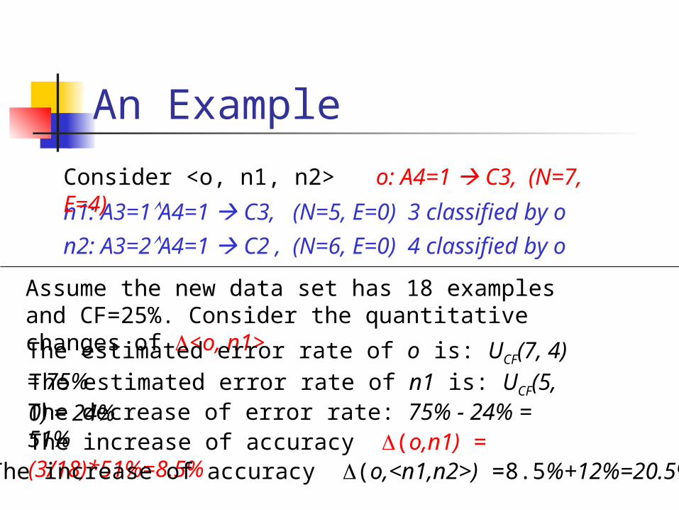
n1: A3=1A4=1 C3, (N=5, E=0) 3 classified by o n2: A3=2A4=1 C2 , (N=6, E=0) 4 classified by o
Consider <o, n1, n2> o: A4=1 C3, (N=7, E=4)
Assume the new data set has 18 examples and CF=25%. Consider the quantitative changes of <o, n1>The estimated error rate of o is: UCF(7, 4) = 75%The estimated error rate of n1 is: UCF(5, 0) = 24%The decrease of error rate: 75% - 24% = 51%The increase of accuracy (o,n1) = (3/18)*51%=8.5%The increase of accuracy (o,<n1,n2>) =8.5%+12%=20.5%

Types of Changes Global changes: both
characteristics change and quantitative change are large.
Alternative changes: characteristics change is large but its quantitative change is small.

Types of Changes (Cont.) Target changes: similar
characteristics but different classes (targets)
Interval changes: shift of boundary points due to the emerging of new cutting points.

Experiments Two data sets:
German Credit Data from UCI repository [MM96]
IPUMS Census Data [IPUMS] Goal: to verify if our algorithm can
find the important changes “supposed” to be found

Methodologies For German Credit data:
Plant some changes to original data and check if the proposed method finds them.
For IPUMS census data: The proposed method is applied to find
the changes across years or different sub-populations.
Classifiers are built using C4.5 algorithm

Summaries of German Data Data description:
2 classes: bad and good 20 attributes, 13 categorical 1000 examples: 700 are “good”
Changes planted: Target change Interval change Etc.

Planting Target Change
Personal-status = single-male, Foreign = no Credit = good (23, 0)
Changes planted: if ( Liable-people=1 ) then change the class from good to bad
12 examples changed
Consider the examples classified by the old rule.

The Changes Found
Personal-status = single-male, Foreign = no Credit = good
Liable-people >1, Foreign = no Credit = good( = 0.54%)
Personal-status = single-male, Liable-people <=1, Foreign = no Credit = bad ( = 0.48%)

Planting Interval Change
Status = 0DM, Duration > 11, Foreign = yes Credit = bad (164, 47)
Changes planted: Increase the Duration value by 6 (months) for each example classified by the old rule.
164 examples changed
Consider the examples classified by the old rule.

The Changes Found
Status = 0DM, Duration > 11, Foreign = yes Credit = bad
Status = 0DM,Duration > 16, Foreign = yes
Credit = bad( = 1.20%)

Summaries of IPUMS Data Take “vetstat” as class 3 data sets: 1970, 1980 and 1990. Each data set contains the
examples for several races. The proposed method is applied to
find the changes across years or different sub-populations.

Interesting Changes Found
35<age ≤54 Vetstat=yes
40<age ≤72, sex=male Vetstat=yes( = 1.20%)
A. 1970-black vs 1990-black
40<age ≤72, sex=male Vetstat=yes
bplg =china, incss ≤5748 Verstat=no( = 4.56%)
B. 1990-black vs 1990-chinese

Conclusion Extracting changes from potentially
very dissimilar old and new classifiers by correspondence tracing
Ranking the importance of changes Presenting the changes Experiments on real-life data sets

References [GGR99] V. Ganti, J. Gehrke, and R.
Ramakrishnan. A framework for measuring changes in data characteristics. In PODS, 1999
[IPUMS] http://www.ipums.umn.edu/.
[LHHX00] B. Liu,W. Hsu, H.S. Han, and Y. Xia. Mining changes for real-life applications. In DaWak, 2000

References (Cont.) [MM96] C.J. Merz and P. Murphy.
UCI repository of machine learning databases
[Q93] J.R. Quinlan. C4.5: programs for maching learning. 1993


![An Immersive System with Multi-modal Human-computer ...cvrl/wangk/papers/Zhao2018a.pdf · [23] applied the full immersive environment CAVE [15] to education in chemistry by visualizing](https://cdn.vdocuments.us/doc/165x107/5e0bace90fda4756121ad7ae/an-immersive-system-with-multi-modal-human-computer-cvrlwangkpapers-23.jpg)


