
11
Minimum-Energy Motion Planning for Differential-Driven Wheeled Mobile Robots
Chong Hui Kim1 and Byung Kook Kim2 1Agency for Defense Development,
2School of Electrical Engineering and Computer Science, KAIST Republic of Korea
1. Introduction
With the remarkable progresses in robotics, mobile robots can be used in many applications including exploration in unknown areas, search and rescue, reconnaissance, security, military, rehabilitation, cleaning, and personal service. Mobile robots should carry their own energy source such as batteries which have limited energy capacity. Hence their applications are limited by the finite amount of energy in the batteries they carry, since a new supply of energy while working is impossible, or at least too expensive to be realistic. ASIMO, Honda’s humanoid robot, can walk for only approximately 30 min with its rechargeable battery backpack, which requires four hours to recharge (Aylett, 2002). The BEAR robot, designed to find, pick up, and rescue people in harm’s way, can operate for approximately 30 min (Klein et al., 2006). However, its operation time is insufficient for complicated missions requiring longer operation time. Since operation times of mobile robots are mainly restricted by the limited energy capacity of the batteries, energy conservation has been a very important concern for mobile robots (Makimoto & Sakai, 2003; Mei et al., 2004; Spangelo & Egeland, 1992; Trzynadlowski, 1988; Zhang et al., 2003). Rybski et al. (Rybski et al., 2000) showed that power consumption is one of the major issues in their robot design in order to survive for a useful period of time. Mobile robots usually consist of batteries, motors, motor drivers, and controllers. Energy conservation can be achieved in several ways, for example, using energy-efficient motors, improving the power efficiency of motor drivers, and finding better trajectories (Barili et al., 1995; Mei et al., 2004; Trzynadlowski, 1988; Weigui et al., 1995). Despite efficiency improvements in the motors and motor drivers (Kim et al., 2000; Leonhard, 1996), the operation time of mobile robots is still limited in their reliance on batteries which have finite energy. We performed experiments with mobile robot called Pioneer 3-DX (P3-DX) to measure the power consumption of components: two DC motors and one microcontroller which are major energy consumers. Result shows that the power consumption by the DC motors accounts for more than 70% of the total power. Since the motor speed is largely sensitive to torque variations, the energy dissipated by a DC motor in a mobile robot is critically dependent on its velocity profile. Hence energy-optimal motion planning can be achieved by determining the optimal velocity profile and by controlling the mobile robot to follow that trajectory, which results in the longest working time possible.
www.intechopen.com
Mobile Robots Motion Planning, New Challenges
194
The total energy drawn from the batteries is converted to mechanical energy by driving motors, which is to induce mobile robot’s motion with some losses such as armature heat dissipation by the armatures in the motors. The DC motor is most widely used to produce mechanical power from electric power. It converts electric power into mechanical power during acceleration and cruise. Moreover, during deceleration, mechanical energy can be converted back to electrical energy (Electro-Craft, 1977). However, the motor is not an ideal energy converter, due to losses caused by the armature resistance, the viscous friction, and many other loss components. Many researchers have concentrated on minimizing losses of a DC motor (Trzynadlowski, 1988; Angelo et al., 1999; Egami et al., 1990; El-satter et al., 1995; Kusko & Galler, 1983; Margaris et al., 1991; Sergaki et al., 2002; Tal, 1973). They developed cost function in terms of the energy loss components in a DC motor in order to conserve limited energy. The loss components in a DC motor include the armature resistance loss, field resistance loss, armature iron loss, friction and windage losses, stray losses, and brush contact loss. Since it is difficult to measure all the parameters of the loss components, its implementation is relatively complex. To overcome this problem, some researches considered only the armature resistance loss as a cost to be minimized (Trzynadlowski, 1988; Tal, 1973; Kwok & Lee, 1990). However, loss-minimization control is not the optimal in terms of the total energy drawn from the batteries. Control of wheeled mobile robot (WMR) is generally divided into three categories (Divelbiss & Wen, 1997).
• Path Planning: To generate a path off-line connecting the desired initial and final configurations with or without obstacle avoidance.
• Trajectory Generation: To impose a velocity profile to convert the path to a trajectory.
• Trajectory Tracking: To make a stable control for mobile robots to follow the given trajectory.
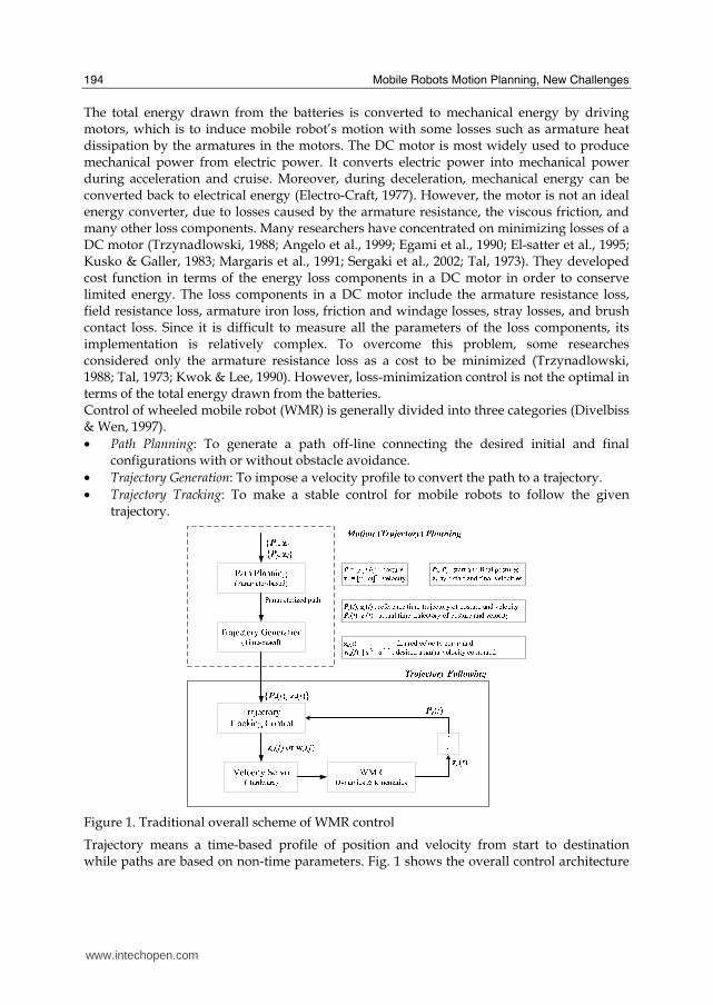
Figure 1. Traditional overall scheme of WMR control
Trajectory means a time-based profile of position and velocity from start to destination while paths are based on non-time parameters. Fig. 1 shows the overall control architecture
www.intechopen.com
Minimum-Energy Motion Planning for Differential-Driven Wheeled Mobile Robots
195
of WMR system (Choi, 2001). Finding a feasible trajectory is called trajectory planning or motion planning (Choset et al., 2005). Trajectory planning (motion planning) is a difficult problem since it requires simultaneously solving the path planning and velocity planning (trajectory generation) problems (Fiorini & Shiller, 1998). Most of the paths of WMR consist of straight lines and arcs. The pioneering work by Dubins (Dubins, 1957) and then by Reeds and Shepp (Reeds & Shepp, 1990) showed that the shortest paths for car-like vehicle were made up of straight lines and circular arcs. Since these paths generate discontinuities of curvature at junctions between line and arc segment, a real robot would have to stop at each curvature discontinuity. Hence frequent stops and turnings cause unnecessary acceleration and deceleration that consume significant battery energy. In order to remove discontinuity at the line-arc transition points, several types of arcs have been proposed. Clothoid and cubic spirals provide smooth transitions (Kanayama & Miyake, 1985; Kanayama & Harman, 1989). However, these curves are described as functions of the path-length and it is hard to consider energy conservation and dynamics of WMR. Barili et al. described a method to control the travelling speed of mobile robot to save energy (Barili et al., 1995). They considered only straight lines and assumed constant acceleration rate. Mei et al. presented an experimental power model of mobile robots as a function of constant speed and discussed the energy efficiency of the three specific paths (Mei et al., 2004; Mei et al., 2006). They did not consider arcs and the energy consumption in the transient sections for acceleration and deceleration to reach a desired constant speed. In this book chapter, we derive a minimum-energy trajectory for differential-driven WMR that minimizes the total energy drawn from the batteries, using the actual energy consumption from the batteries as a cost function. Since WMR mainly moves in a straight line and there is little, if any, rotation (Barili et al., 1995; Mei et al., 2005), first we investigate minimum-energy translational trajectory generation problem moving along a straight line. Next we also investigate minimum-energy turning trajectory planning problem moving along a curve since it needs turning trajectory as well as translational trajectory to do useful actions. To demonstrate energy efficiency of our trajectory planner, various simulations are performed and compared with loss-minimization control minimizing armature resistance loss. Actual experiments are also performed using a P3-DX mobile robot to validate practicality of our algorithm. The remainder of the book chapter is organized as follows. Section 2 gives the kinematic and dynamic model of WMR and energy consumption model of WMR. In Section 3, we formulate the minimum-energy translational trajectory generation problem. Optimal control theory is used to find the optimal velocity profile in analytic form. Experimental environment setup to validate simulation results is also presented. In Section 4, we formulate the minimum-energy turning trajectory planning problem and suggest iterative search algorithm to find the optimal trajectory based on the observation of the cost function using the solution of Section 3. Finally, we conclude with remarks in Section 5.
2. WMR Model
2.1 Kinematic and Dynamic Model of WMR
It is well known that a WMR is a nonholonomic system. A full dynamical description of such nonholonomic mechanical system including the constraints and the internal dynamics can be found in (Campion et al., 1991). Yun (Yun, 1995; Yun & Sarkar, 1998) formulated a dynamic system with both holonomic and nonholonomic constraints resulting from rolling contacts into the standard control system form in state space. Kinematic and dynamic
www.intechopen.com
Mobile Robots Motion Planning, New Challenges
196
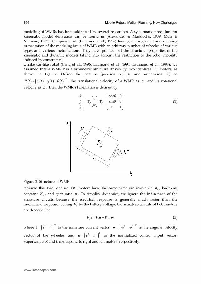
modeling of WMRs has been addressed by several researches. A systermatic procedure for kinematic model derivation can be found in (Alexander & Maddocks, 1989; Muir & Neuman, 1987). Campion et al. (Campion et al., 1996) have given a general and unifying presentation of the modeling issue of WMR with an arbitrary number of wheeles of various types and various motorizations. They have pointed out the structural properties of the kinematic and dynamic models taking into account the restriction to the robot mobility induced by constraints. Unlike car-like robot (Jiang et al., 1996; Laumond et al., 1994; Laumond et al., 1998), we assumed that a WMR has a symmetric structure driven by two identical DC motors, as
shown in Fig. 2. Define the posture (position x , y and orientation ┠ ) as
( ) ( ) ( ) ( )= ⎡ ⎤⎣ ⎦Tt x t y t ┠ tP , the translational velocity of a WMR as v , and its rotational
velocity as ω . Then the WMR’s kinematics is defined by
⎡ ⎤ ⎡ ⎤⎡ ⎤⎢ ⎥ ⎢ ⎥= =⎢ ⎥⎢ ⎥ ⎢ ⎥⎣ ⎦⎢ ⎥ ⎢ ⎥⎣ ⎦⎣ ⎦
$$$
cos 0
, sin 0
0 1P P
x ┠v
y ┠ω
┠T T (1)
Figure 2. Structure of WMR
Assume that two identical DC motors have the same armature resistance aR , back-emf
constant bK , and gear ratio n . To simplify dynamics, we ignore the inductance of the
armature circuits because the electrical response is generally much faster than the
mechanical response. Letting sV be the battery voltage, the armature circuits of both motors
are described as
= −a s bR V K ni u w (2)
where ⎡ ⎤= ⎣ ⎦TR Li ii is the armature current vector, ⎡ ⎤= ⎣ ⎦TR Lω ωw is the angular velocity
vector of the wheeles, and ⎡ ⎤= ⎣ ⎦TR Lu uu is the normalized control input vector.
Superscripts R and L correspond to right and left motors, respectively.
www.intechopen.com

Minimum-Energy Motion Planning for Differential-Driven Wheeled Mobile Robots
197
In addition, the dynamic relationship between angular velocity and motor current, considering inertia and viscous friction, becomes (Yun & Yamamoto, 1993)
+ =v t
dF K n
dtJ
ww i (3)
where vF is the viscous friction coefficient and equivalent inertia matrix of motors J is
= TJ S MS , which is 2x2 symmetric.
From Eqs. (2) and (3), we obtain the following differential equation.
+ =$w Aw Bu (4)
where
− ⎛ ⎞⎡ ⎤= = +⎜ ⎟⎢ ⎥⎣ ⎦ ⎝ ⎠
21 2 1
2 1
t bv
a
a a K K nF
a a RA J , −⎡ ⎤
= =⎢ ⎥⎣ ⎦1 2 1
2 1
s t
a
b b V K n
b b RB J
Define a state vector as [ ]=T
v ωz . Then v and ω are related to Rω and Lω by
⎡ ⎤⎡ ⎤
= = =⎢ ⎥⎢ ⎥⎣ ⎦ ⎣ ⎦R
q qL
v ωω ω
z T T w , ⎡ ⎤
= ⎢ ⎥−⎣ ⎦/2 /2
/2 /2q
r r
r b r bT (5)
Using the similarity transformation, from Eqs. (4) and (5), we obtain the following equation
+ =$z Az Bu (6)
where
1 21
1 2
0 0
0 0v
q qω
┨ a a
┨ a a−
+⎡ ⎤ ⎡ ⎤= = =⎢ ⎥ ⎢ ⎥−⎣ ⎦ ⎣ ⎦A T AT
( ) ( )( ) ( )
1 1 1 2 1 2
2 2 1 2 1 2
/2 /2
/2 /2q
┚ ┚ r b b r b b
┚ ┚ r b b b r b b b
+ +⎡ ⎤⎡ ⎤= = = ⎢ ⎥⎢ ⎥− − − −⎣ ⎦ ⎣ ⎦B T B
The overall dynamics of a WMR is shown in Fig. 3, where 2I is the 2x2 unit matrix.
Figure 3. Block diagram of WMR
2.2 Energy Consumption of WMR
The energy drawn from the batteries is converted to mechanical energy to drive motors and losses such as the heat dissipation in the armature resistance. In a WMR, energy is
www.intechopen.com

Mobile Robots Motion Planning, New Challenges
198
dissipated by the internal resistance of batteries, amplifier resistance in motor drivers, armature resistance, and viscous friction of motors. Fig. 4 shows a simplified circuit diagram of a WMR system.
Figure 4. Circuit diagram of batteries, motor drivers, and motors of WMR
A pulse width modulated (PWM) controller is the preferred motor speed controller because little heat is generated and it is energy efficient compared to linear regulation (voltage control) of the motor. We assume that an H-bridge PWM amplifier is used as a motor driver,
and this is modeled by its amplifier resistance RAMP and PWM duty ratio Ru and Lu . In our
robot system, P3-DX, internal resistance of battery (CF-12V7.2) is approximately 22mΩ and power consumption by the motor drivers is 0.2W. Since internal resistance of battery is
much smaller compared with armature resistance of motor (710mΩ) and the power consumption by the motor drivers is much smaller than that of motors (several watts), they are ignored here. Hence the total energy supplied from the batteries to the WMR, EW, is the cost function to be minimized and is defined as
T TW sE dt V dt= =∫ ∫i V i u (7)
where TR LV V⎡ ⎤= ⎣ ⎦V is the input voltage applied to the motors from the batteries, and
/TR L
sV u u⎡ ⎤= = ⎣ ⎦u V .
As there is a certain limit on a battery’s output voltage, WMR systems have a voltage constraint on batteries:
max maxRu u u− ≤ ≤ , max maxLu u u− ≤ ≤ (8)
www.intechopen.com

Minimum-Energy Motion Planning for Differential-Driven Wheeled Mobile Robots
199
From Eqs. (2) and (5), EW can be written in terms of the velocity and the control input as
( )1 2T T T
W qE k k dt−= −∫ u u z T u (9)
where 21 /s ak V R= and 2 /b s ak K nV R= .
From Eqs. (2) and (3), the cost fuction EW becomes
1 1T T T T T Tb bW a v q q q q
t t
K KE R dt F dt dt
K K− − − −= + +∫ ∫ ∫i i z T T z z T J T z$ (10)
Note that the first term, ( )TR aE R dt= ∫ i i , is the energy dissipated by the armature resistance
in the motors and the cost function of loss-minimization control considering only the
armature resistance loss. The second term, 1T TbF v q q
t
KE F dt
K− −⎛ ⎞
=⎜ ⎟⎝ ⎠∫z T T z , corresponds to the
velocity sensitive loss due to viscous friction. The last term, 1T T TbK q q
t
KE dt
K− −⎛ ⎞
=⎜ ⎟⎝ ⎠∫z T J T z$ , is the
kinetic energy stored in the WMR and will have zero average value when the velocity is constant or final velocity equal to the initial velocity. This means that the net contribution of the last term to the energy consumption is zero.
3. Minimum-Energy Translational Trajectory Generation
A mobile robot’s path usually consists of straight lines and arcs. In the usual case, a mobile robot mainly moves in a straight line and there is little, if any, rotation (Barili et al., 1995; Mei et al., 2005). Since the energy consumption associated with rotational velocity changes is much smaller than the energy consumption associated with translational velocity changes, we investigate minimum-energy translational trajectory generation of a WMR moving along a straight line. Since the path of WMR is determined as a straight line, this problem is reduced to find velocity profile minimizing energy drawn from the batteries.
3.1 Problem Statement
The objective of optimal control is to determine the control variables minimizing the cost function for given constraints. Because the rotational velocity of WMR, ω , is zero under
translational motion constraint, let ( ) ( ) 0 0T
t x t= ⎡ ⎤⎣ ⎦P be the posture and
( ) ( ) 0T
t v t= ⎡ ⎤⎣ ⎦z be the velocity at time t . Then the minimum-energy translational trajectory
generation problem investigated in this section can be formulated as follows.
Problem: Given initial and final times 0t and ft , find the translational velocity ( )v t and the
control input ( )u t which minimizes the cost function
( )0
1 2
ftT T T
W qt
E k k dt−= −∫ u u z T u
www.intechopen.com
Mobile Robots Motion Planning, New Challenges
200
for the system described by Eq. (6) subject to
(1) initial and final postures: ( ) [ ]0 0 0 0T
t x=P and ( ) 0 0T
f ft x⎡ ⎤= ⎣ ⎦P ,
(2) initial and final velocities: ( ) [ ]0 0T
st v=z and ( ) 0T
f ft v⎡ ⎤= ⎣ ⎦z , and
(3) satisfying the batteries’ voltage constraints, maxu
As time is not critical, a fixed final time is used.
3.2 Minimum-Energy Translational Trajectory
Without loss of generality, we assume that the initial and final velocities are zero, and the initial posutre is zero. Then the minimum-energy translational trajectory generation problem can be written as
minimize ( )1 20
ftT T
W qE k k dt−= −∫ u u zT u (11)
subject to = − +z Az Bu$ (12)
( ) ( ) [ ]0 0 0T
ft= =z z (13)
0
0 0ft T
f P fP dt x⎡ ⎤= = ⎣ ⎦∫ T z (14)
max max
max max
R
L
u u u
u u u
⎡ ⎤ ⎡ ⎤ ⎡ ⎤−≤ = ≤⎢ ⎥ ⎢ ⎥ ⎢ ⎥
−⎣ ⎦ ⎣ ⎦ ⎣ ⎦u (15)
We used the Pontryagin’s Maximum Principle to find the minimum-energy velocity profile that minimizes Eq. (11) while satisfying the constraints in Eqs. (13) – (15) for the system, with Eq. (12). Let the Largrange multiplier for the posture constraint, Eq. (14), be
T
x y ┠┙ ┙ ┙⎡ ⎤= ⎣ ⎦α . Defining the multipler function for Eq. (12) as, [ ]T
v ωλ λ=λ , the
Hamiltonian H is
( )1 2 /T T T T T Tq p f fH k k t−= − − + + − +u u z T u α T z α λ Az BuP (16)
The necessary conditions for the optimal velocity *z and the control input *u are
11 2/ 2 0T
qH k k −∂ ∂ = − + =u u T z B λ (17)
2/ T T Tq PH k −∂ ∂ = − − − = −z T u T α A λ λ$ (18)
/H∂ ∂ = − + =λ Az Bu z$ (19)
From Eqs. (17) – (19), we obtain the following differential equation.
1 12
1 1
10
2T T T T T T T
q P
k
k k− − − −⎛ ⎞
− − + =⎜ ⎟⎝ ⎠z BB A B B A BB T B A z BB T α$$ (20)
www.intechopen.com

Minimum-Energy Motion Planning for Differential-Driven Wheeled Mobile Robots
201
As TBB and A are diagonal matrices, Eq. (20) is reduced to quadratic differential form as follows.
0T T TP− + =z Q Qz R T α$$ (21)
where 12
1
T T T Tq
k
k− −= −Q Q A A BB T B A ,
1/ 0
0 1/v
ω
ττ
⎡ ⎤= ⎢ ⎥⎣ ⎦Q , and
1
0
02
Tv
ω
┟┟k
⎡ ⎤= = ⎢ ⎥⎣ ⎦
B BR . Here
( ) ( )21 2 / /v v v t b aτ J J F F K K n R= + + denotes the mechanical time constant for translation and
( ) ( )21 2 / /ω v v t b aτ J J F F K K n R= − + denotes the mechanical time constant for rotation of WMR.
Since we ignore energy dissipation associated with rotational velocity changes and consider only a WMR moving along a straight line (i.e., rotational velocity is zero), the optimal
velocity *z becomes
( )( )
( )
* / /1 2*
* 0
v vt τ t τvv t C e C e K
tω t
−⎡ ⎤ ⎡ ⎤+ += =⎢ ⎥ ⎢ ⎥⎣ ⎦ ⎣ ⎦z (22)
where
/
1 / /
1f v
f v f v
t τ
vt τ t τe
C Ke e
−
−
−=
−,
/
2 / /
1 f v
f v f v
t τ
vt τ t τe
C Ke e
−
−=
−,
( )( ) ( )
/ /
/ / / /2 2
f v f v
f v f v f v f v
t τ t τf
v t τ t τ t τ t τv f
x e eK
τ e e t e e
−
− −
−=
− − + −
To investigate the properties of the minimum-energy velocity profile, the minimum-energy translational velocity profile, Eq. (22), is shown in Fig. 5 as velocity per unit versus time per
unit, where the reference velocity is taken as the /f fx t ratio and the reference time / ft t for
various /v fk τ t= (the ratio of translational mechanical time constant per displacement time)
using the parameters shown in Table 1.
0 0.2 0.4 0.6 0.8 10
0.2
0.4
0.6
0.8
1
1.2
1.4
1.6
Time, P. U.
Tra
nsl
ati
on
al
Vel
oci
ty,
P.
U.
k=0.01k=0.05k=0.10k=0.20k=0.50
Figure 5. Minimum-Energy velocity profiles for incremental motion at various /v fk τ t=
www.intechopen.com

Mobile Robots Motion Planning, New Challenges
202
Parameter Value Parameter Value
aR 0.71Ω tK 0.023Nm/A
bK 0.023V/(rad/s) n 38.3
cm 13.64Kg ωm 1.48Kg
sV 12.0V maxu 1.0
vF 0.039Nm/(rad/s) r 0.095m
b 0.165m 1 2
2 1
J J
J J
⎡ ⎤= ⎢ ⎥⎣ ⎦J
0.0799 0.0017
0.0017 0.0799
⎡ ⎤⎢ ⎥⎣ ⎦
Table 1. Parameters of the WMR, P3-DX
This shows that for k close to zero the minimum-energy velocity profile resembles a widely
used trapezoidal velocity profile, whereas for values of 0.2k > the profile rapidly converges
to a parabolic profile instead of the widely used trapezoidal profile. As shown in Fig. 5, the minimum-energy velocity profile has a symmetric form for the minimum-energy translational trajectory generation problem, of Eqs. (11) – (15) as follows.
( )( ) ( )( ) ( )
( )( ) ( )
*sinh / sinh / sinh /
2 1 cosh / sinh /
f v f v vf
fvf v f v
v
t τ t t τ t τxv t
tτt τ t τ
τ
− − −=
− +
(23)
Eq. (23) means that the minimum-energy velocity profile depends on the ratio of the
mechanical time constant vτ and the displacement time ft .
3.3 Simulations and Experiments
3.3.1 Simulations
Several simulations were performed to evaluate the energy saving of the minimum-energy
control optimizing the cost function WE of Eq. (11); these were compared with two results
of other methods: loss-minmization control (Trzynadlowski, 1988; Tal, 1973; Kwok & Lee,
1990) optimizing energy loss due to armature resistance of a DC motor, ( )TR aE R dt= ∫ i i , and
the fixed velocity profile of commonly used trapezoidal velocity profile optimizing the cost
function WE of Eq. (11).
Table 3.2 shows the simulation results of the energy saving for various displacements fx
and displacement time ft . Minimum-Energy denotes the mnimum-energy control
optimizing the cost fucntion WE , Loss-Minimization denotes the loss-minimization control
optimizing the cost function RE , and TRAPE denotes the trapezoidal velocity profile
optimizing the cost fuction WE . Values in parenthesis represent percentage difference in the
total energy drawn from the batteries with respect to that of minimum-energy control. It shows that minimum-energy control can save up to 8% of the energy drawn from the batteries compared with loss-minimization control and up to 6% compared with energy-optimal trapezoidal velocity profile. Because the minimum-energy velocity profile of Eq. (23) resembles a trapezoid for a sufficiently long displacement time, the energy-optimal
www.intechopen.com

Minimum-Energy Motion Planning for Differential-Driven Wheeled Mobile Robots
203
trapezoidal velocity profile converges to minimum-energy velocity profile and is a near energy-optimal velocity profile for a longer displacement time. However, it expends more energy when frequent velocity changes are required due to obstacles.
Constraints Total Energy Drawn from the Batteries WE (J)
ft fx Minimum-Energy Loss-Minimization TRAPE
2.0s 1.0m 7.26 7.38 (1.65%) 7.70 (6.06%)
5.0s 3.0m 19.07 20.26 (6.24%) 19.57 (2.62%)
10.0s 5.0m 24.26 26.22 (8.08%) 24.57 (1.27%)
20.0s 10.0m 46.56 49.38 (6.06%) 46.85 (0.62%)
30.0s 15.0m 68.92 71.91 (4.34%) 69.20 (0.41%)
Table 2. Comparison of energy saving for various ft and fx
Compared with loss-minimization control, minimum-energy control has a significant energy saving for a displacement time greater than 2s. For a further investigation, we performed a careful analysis of two optimization problems: minimum-energy control and
loss-minimization control. Fig. 6 shows the simulations for various time constants vτ that
were performed for tf = 10.0s and xf = 5.0m. As the energy-optimal velocity profile depends
on = /v fk τ t , as shown in Fig. 5, the mechanical time constant affects the velocity profiles of
the two optimization problems with different cost functions.
0 1 2 3 4 50
5
10
15
20
25
30
Mechanical Time Constant τ
En
erg
y D
raw
n f
rom
Ba
tter
ies
[J]
τ Minimum-Energy
τ Loss-Minimization
EW
ER
EF
Figure 6. Cost function plot with respect to mechanical time constant τ
Applying the Pontryagin’s Maximum Princple to optimize the cost function, the mechanical
time constants are ( ) ( )= + + 21 2 / /v v v t b aτ J J F F K K n R for minimum-energy control and
( )= +1 2 /v vτ J J F for loss-minimization control. Fig. 6 shows the change of the cost function
with respect to various mechanical time constant τ .
From Eq. (2), decreasing the armature current increases the value of the back-emf and the motor speed. Because the mechanical time constant of minimum-energy control less than that of loss-minimization control, the armature current in minimum-energy control quickly
www.intechopen.com

Mobile Robots Motion Planning, New Challenges
204
decreases, as shown in Fig. 7(c) during acceleration and deceleration. Hence minimum-energy control can accelerate and decelerate at a higher acceleration rate as shown in Fig. 7(a). Corresponding control inputs are shown in Fig. 7(b) and energy consumptions for each case are shown in Fig. 7(d).
0 2 4 6 8 100
0.1
0.2
0.3
0.4
0.5
0.6
0.7
0.8
Time [s]
Tra
nsl
ati
on
al
Vel
oci
ty [
m/s
]
Optimal Velocity Profile
Minimum-Energy
Loss-Minimization
0 2 4 6 8 10
-0.1
0
0.1
0.2
0.3
0.4
0.5
0.6
Time [s]
No
rma
lize
d C
on
tro
l In
pu
t
Control Input ( u = uR
= uL
)
Minimum-Energy
Loss-Minimization
(a) (b)
0 2 4 6 8 10-1.5
-1
-0.5
0
0.5
1
1.5
Time [s]
Arm
atu
re C
urr
ent
[A]
Armature Current ( i = iR
= iL)
Minimum-Energy
Loss-Minimization
0 2 4 6 8 10
0
5
10
15
20
25
30
Time [s]
Dra
wn
Ba
tter
y E
ner
gy
[J
]
Total Energy drawn from Batterries
Minimum-Energy
Loss-Minimization
(c) (d)
Figure 7. Simulations of minimum-energy control and loss-minimization control for tf = 10.0s and xf = 5.0m, (a) Optimal velocity profile, (b) Corresponding control inputs, (c) Armature current change, (d) Comparison of energy consumption
Table 3 shows the ratio of consumed energy for each energy component of Eq. (10) with respect to total energy drawn from the batteries during the entire process for minimum-energy control. Note that the kinetic energy acquired at start up is eventually lost to the whole process when the final velocity is equal to the initial velocity, as shown in Table 3.
tf xf EW(%) ER (%) EF (%) EK (%)
2.0s 1.0m 7.26 2.30 (31.68%) 4.96 (68.32%) 0.00 (0.00%)
5.0s 3.0m 19.07 2.35 (12.32%) 16.72 (87.68%) 0.00 (0.00%)
10.0s 5.0m 24.26 1.82 (7.50%) 22.44 (92.50%) 0.00 (0.00%)
20.0s 10.0m 46.56 2.51 (5.39%) 44.05 (94.61%) 0.00 (0.00%)
30.0s 15.0m 68.92 3.26 (4.73%) 65.66 (95.27%) 0.00 (0.00%)
Table 3. Ratio of energy consumption of each energy component for minimum-energy control
www.intechopen.com
Minimum-Energy Motion Planning for Differential-Driven Wheeled Mobile Robots
205
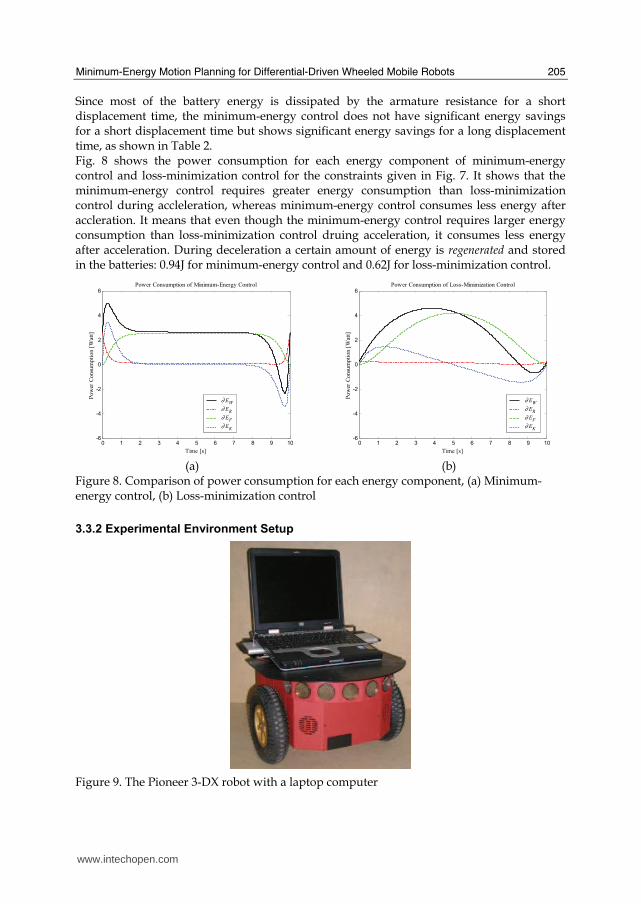
Since most of the battery energy is dissipated by the armature resistance for a short displacement time, the minimum-energy control does not have significant energy savings for a short displacement time but shows significant energy savings for a long displacement time, as shown in Table 2. Fig. 8 shows the power consumption for each energy component of minimum-energy control and loss-minimization control for the constraints given in Fig. 7. It shows that the minimum-energy control requires greater energy consumption than loss-minimization control during accleleration, whereas minimum-energy control consumes less energy after accleration. It means that even though the minimum-energy control requires larger energy consumption than loss-minimization control druing acceleration, it consumes less energy after acceleration. During deceleration a certain amount of energy is regenerated and stored in the batteries: 0.94J for minimum-energy control and 0.62J for loss-minimization control.
0 1 2 3 4 5 6 7 8 9 10-6
-4
-2
0
2
4
6
Time [s]
Po
wer
Co
nsu
mp
tio
n [
Wat
t]
Power Consumption of Minimum-Energy Control
∂ EW
∂ ER
∂ EF
∂ EK
0 1 2 3 4 5 6 7 8 9 10
-6
-4
-2
0
2
4
6
Time [s]
Po
wer
Co
nsu
mp
tio
n [
Wat
t]
Power Consumption of Loss-Minimization Control
∂ EW
∂ ER
∂ EF
∂ EK
(a) (b)
Figure 8. Comparison of power consumption for each energy component, (a) Minimum-energy control, (b) Loss-minimization control
3.3.2 Experimental Environment Setup
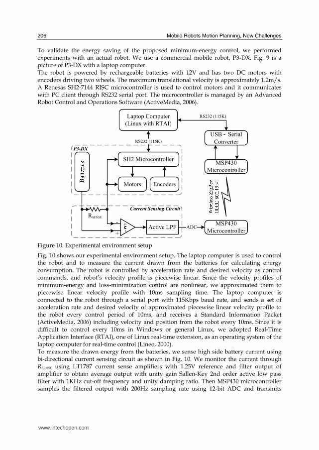
Figure 9. The Pioneer 3-DX robot with a laptop computer
www.intechopen.com
Mobile Robots Motion Planning, New Challenges
206
To validate the energy saving of the proposed minimum-energy control, we performed experiments with an actual robot. We use a commercial mobile robot, P3-DX. Fig. 9 is a picture of P3-DX with a laptop computer. The robot is powered by rechargeable batteries with 12V and has two DC motors with encoders driving two wheels. The maximum translational velocity is approximately 1.2m/s. A Renesas SH2-7144 RISC microcontroller is used to control motors and it communicates with PC client through RS232 serial port. The microcontroller is managed by an Advanced Robot Control and Operations Software (ActiveMedia, 2006).
Current Sensing Circuit
P3-DX
RSENSE
SH2 Microcontroller
Motors Encoders
Laptop Computer
(Linux with RTAI)
+
-Active LPF
MSP430
MicrocontrollerADC
RS232 (115K)
RS232 (115K)
USB – Serial
Converter
MSP430
Microcontroller
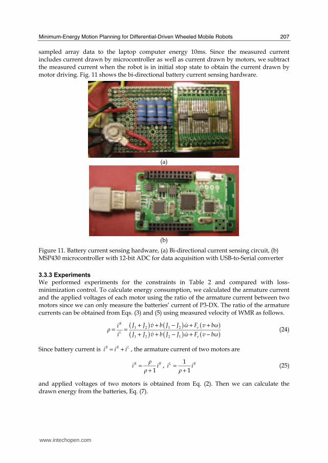
Figure 10. Experimental environment setup
Fig. 10 shows our experimental environment setup. The laptop computer is used to control the robot and to measure the current drawn from the batteries for calculating energy consumption. The robot is controlled by acceleration rate and desired velocity as control commands, and robot’s velocity profile is piecewise linear. Since the velocity profiles of minimum-energy and loss-minimization control are nonlinear, we approximated them to piecewise linear velocity profile with 10ms sampling time. The laptop computer is connected to the robot through a serial port with 115Kbps baud rate, and sends a set of acceleration rate and desired velocity of approximated piecewise linear velocity profile to the robot every control period of 10ms, and receives a Standard Information Packet (ActiveMedia, 2006) including velocity and position from the robot every 10ms. Since it is difficult to control every 10ms in Windows or general Linux, we adopted Real-Time Application Interface (RTAI), one of Linux real-time extension, as an operating system of the laptop computer for real-time control (Lineo, 2000). To measure the drawn energy from the batteries, we sense high side battery current using bi-directional current sensing circuit as shown in Fig. 10. We monitor the current through RSENSE using LT1787 current sense amplifiers with 1.25V reference and filter output of amplifier to obtain average output with unity gain Sallen-Key 2nd order active low pass filter with 1KHz cut-off frequency and unity damping ratio. Then MSP430 microcontroller samples the filtered output with 200Hz sampling rate using 12-bit ADC and transmits
www.intechopen.com
Minimum-Energy Motion Planning for Differential-Driven Wheeled Mobile Robots
207
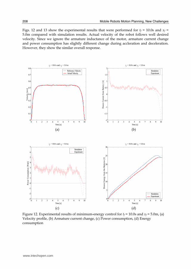
sampled array data to the laptop computer energy 10ms. Since the measured current includes current drawn by microcontroller as well as current drawn by motors, we subtract the measured current when the robot is in initial stop state to obtain the current drawn by motor driving. Fig. 11 shows the bi-directional battery current sensing hardware.
(a)
(b)
Figure 11. Battery current sensing hardware, (a) Bi-directional current sensing circuit, (b) MSP430 microcontroller with 12-bit ADC for data acquisition with USB-to-Serial converter
3.3.3 Experiments
We performed experiments for the constraints in Table 2 and compared with loss-minimization control. To calculate energy consumption, we calculated the armature current and the applied voltages of each motor using the ratio of the armature current between two motors since we can only measure the batteries’ current of P3-DX. The ratio of the armature currents can be obtained from Eqs. (3) and (5) using measured velocity of WMR as follows.
( ) ( ) ( )
( ) ( ) ( )1 2 1 2
1 2 2 1
Rv
Lv
J J v b J J ω F v bωi┩i J J v b J J ω F v bω
+ + − + += =
+ + − + −
$ $$ $
(24)
Since battery current is = +B R Li i i , the armature current of two motors are
1
R B┩i i
┩=
+, =
+
1
1L Bi i
┩ (25)
and applied voltages of two motors is obtained from Eq. (2). Then we can calculate the drawn energy from the batteries, Eq. (7).
www.intechopen.com
Mobile Robots Motion Planning, New Challenges
208
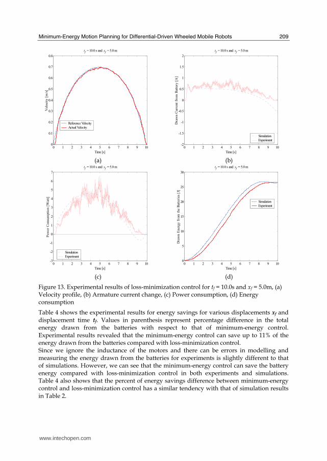
Figs. 12 and 13 show the experimental results that were performed for tf = 10.0s and xf = 5.0m compared with simulation results. Actual velocity of the robot follows well desired velocity. Since we ignore the armature inductance of the motor, armature current change and power consumption has slightly different change during accleration and deceleration. However, they show the similar overall response.
0 1 2 3 4 5 6 7 8 9 100
0.1
0.2
0.3
0.4
0.5
0.6
0.7
0.8
Time [s]
Vel
oci
ty [
m/s
]
tf = 10.0 s and x
f = 5.0 m
Reference Velocity
Actual Velocity
0 1 2 3 4 5 6 7 8 9 10-2
-1.5
-1
-0.5
0
0.5
1
1.5
2
Time [s]
Dra
wn
Cu
rren
t fr
om
Bat
tery
[A
]
tf = 10.0 s and x
f = 5.0 m
Simulation
Experiment
(a) (b)
0 1 2 3 4 5 6 7 8 9 10-3
-2
-1
0
1
2
3
4
5
6
7
Time [s]
Pow
er C
onsu
mp
tion
[W
att]
tf = 10.0 s and x
f = 5.0 m
Simulation
Experiment
0 1 2 3 4 5 6 7 8 9 100
5
10
15
20
25
30
Time [s]
Dra
wn E
ner
gy f
rom
th
e B
atte
ries
[J]
tf = 10.0 s and x
f = 5.0 m
Simulation
Experiment
(c) (d)
Figure 12. Experimental results of minimum-energy control for tf = 10.0s and xf = 5.0m, (a) Velocity profile, (b) Armature current change, (c) Power consumption, (d) Energy consumption
www.intechopen.com
Minimum-Energy Motion Planning for Differential-Driven Wheeled Mobile Robots
209
0 1 2 3 4 5 6 7 8 9 100
0.1
0.2
0.3
0.4
0.5
0.6
0.7
0.8
Time [s]
Vel
oci
ty [
m/s
]
tf = 10.0 s and x
f = 5.0 m
Reference Velocity
Actual Velocity
0 1 2 3 4 5 6 7 8 9 10-2
-1.5
-1
-0.5
0
0.5
1
1.5
2
Time [s]
Dra
wn C
urr
ent
fro
m B
atte
ry [
A]
tf = 10.0 s and x
f = 5.0 m
SimulationExperiment
(a) (b)
0 1 2 3 4 5 6 7 8 9 10-3
-2
-1
0
1
2
3
4
5
6
7
Time [s]
Po
wer
Co
nsu
mpti
on [
Wat
t]
tf = 10.0 s and x
f = 5.0 m
SimulationExperiment
0 1 2 3 4 5 6 7 8 9 100
5
10
15
20
25
30
Time [s]
Dra
wn E
ner
gy
fro
m t
he
Bat
teri
es [
J]
tf = 10.0 s and x
f = 5.0 m
SimulationExperiment
(c) (d)
Figure 13. Experimental results of loss-minimization control for tf = 10.0s and xf = 5.0m, (a) Velocity profile, (b) Armature current change, (c) Power consumption, (d) Energy consumption
Table 4 shows the experimental results for energy savings for various displacements xf and displacement time tf. Values in parenthesis represent percentage difference in the total energy drawn from the batteries with respect to that of minimum-energy control. Experimental results revealed that the minimum-energy control can save up to 11% of the energy drawn from the batteries compared with loss-minimization control. Since we ignore the inductance of the motors and there can be errors in modelling and measuring the energy drawn from the batteries for experiments is slightly different to that of simulations. However, we can see that the minimum-energy control can save the battery energy compared with loss-minimization control in both experiments and simulations. Table 4 also shows that the percent of energy savings difference between minimum-energy control and loss-minimization control has a similar tendency with that of simulation results in Table 2.
www.intechopen.com

Mobile Robots Motion Planning, New Challenges
210
Constraints Total Energy Drawn from the Batteries WE (J)
ft fx Minimum-Energy Loss-Minimization
2.0s 1.0m 8.73 8.97 (2.75%)
5.0s 3.0m 20.42 22.63 (10.82%)
10.0s 5.0m 23.93 26.59 (11.12%)
20.0s 10.0m 45.27 50.16 (10.80%)
30.0s 15.0m 66.61 69.95 (5.01%)
Table 4. Comparison of experimental results of energy saving for various ft and fx
4. Minimum-Energy Turning Trajectory Planning
4.1 Problem Statement
In Section 3, we investigated minimum-energy translational trajectory generation of WMR moving along a straight line. To do useful actions, WMR needs rotational trajectory as well as translational trajectory. According to the configurations of initial and final postures, we can consider two basic paths. The one is single corner path which consists of an approach heading angle followed by a departure heading angle that is along a line at some angle relative to the approach line. That is, it is unnecessary to change the sign of rotational velocity to reach final posture, and the other is double corner path which necessary to change the sign of rotational velocity to reach final posture as shown in Fig. 14. More complicated paths can be constructed by combining multiple single corner paths.
Ps
Pf
(a) (b)
Figure 14. Classification of paths, (a) Single corner path, (b) Double corner path
For simplicity, we consider the single corner path. Futhermore, because of nonlinear and nonholonomic properties, a graphical approach will be used with the following definition about two sections to solve trajectory planning problem.
• Rotational section is a section where the rotational velocity of WMR is not zero, as a result, turning motion is caused.
• Translational section is a section where the rotational velocity is zero, as a result, linear motion is caused only.
Since the paths for single corner are expected to be made up with one rotational section and two translational sections surrounding the rotational section, we divide our trajectory planning algorithm into three sections. The first is RS (rotational section) which is focused on the required turning angle, and the others are TSB (translational section before rotation)
www.intechopen.com

Minimum-Energy Motion Planning for Differential-Driven Wheeled Mobile Robots
211
and TSA (translational section after rotation) which are secondary procedure to satisfy the condition of positions.
TSA
Bac
kw
ard R
ay o
f P
f
Figure 15. Sections in path and requirement of path-deviation
As shown in Fig. 15, let [ ]T
s s s sx y ┠=P and T
f f f fx y ┠⎡ ⎤= ⎣ ⎦P be given initial and final
postures, and [ ]T
m m mx y= −P be the via point which is an intersection of the forward ray
of sP and the backward ray of fP , where ‘-‘ means that value is not used. Since there are
limitations by obstacles or walls in real world, we consider the bound of path-deviation D
(or deviation from the corner, ( )/cos Δ /2cD D ┠= where Δ f s┠ ┠ ┠= − ) as shown in Fig. 15,
which limits path-deviation from the given configuration. In Fig. 15, path-deviation is given considering the safety margin to avoid collisions to the obstacles. Hence the path for single corner is divided into three sections: TSB, RS, and TSA. Then the minimum-energy turning trajectory planning problem can be formulated as follows.
Problem: Given initial and final times 0t and ft , find the trajectory, that is path and velocity
profiles, which minimizes the cost function
( )0
1 2
ftT T T
W qt
E k k dt−= −∫ u u z T u
for the system described by Eq. (6) subject to
(1) initial and final postures: ( )0t = sP P and ( )f ft =P P ,
(2) initial and final velocities: ( )0 st =z z and ( )f ft =z z ,
(3) satisfying the batteries’ voltage constraints maxu , and
(4) satisfying the path-deviation constraint D.
4.2 Minimum-Energy Turning Trajectory Planning 4.2.1 Overview of the Method
WMR’s path is described by finite sequences of two straight lines for translational motions and an arc for rotational motion in between as shown in Fig. 15. The velocity of the WMR
www.intechopen.com
Mobile Robots Motion Planning, New Challenges
212
depends on planning path and the path of the WMR depends on planning velocity profile. Hence energy consumption depends on path and velocity, i.e., the trajectory. We define a
trajectory of the WMR at time t as ( ) ( ) ( )T
t S t ┠ t= ⎡ ⎤⎣ ⎦q , where ( )S t is the displacement
profile of the WMR and ( )┠ t is the orientation profile of the WMR. Since velocity of the
WMR is a time derivative of trajectory, trajectory has the following relationship.
=q z$ or dt= ∫q z (26)
In Fig. 15, let RsP and RfP be start and end postures of RS, and velocities at RsP and RfP be
zRs and zRf , respectively. Without loss of generality, we stipulate that initial posture is
[ ]0 0 0T
s =P , and the initial and final velocities are ( ) ( ) [ ]0 0 0T
ft t= =z z . We define the
velocities at tRs and tRf are ( ) [ ]0T
Rs Rs Rst v= =z z and ( ) 0T
Rf Rf Rft v⎡ ⎤= =⎣ ⎦z z ,
respectively. Then the velocity profile has a shape as shown in Fig. 16.
v(t)
(t)
TSB RS TSA
ts=0 tRs tRf tf
vRs
vRf
vs = vf
TTSB TRS TTSA Time
Time
Translation with
AccelerationRotation
Translation with
Deceleration
Figure 16. Possible shape of the velocity profile for single corner trajectory
The tRs and tRf denote initial and final time of RS. We define a time interval of TSB as
0TSB RsT t T= − , a time interval of RS as RS Rf RsT t t= − , and a time interval of TSA as
TSA f RfT t t= − .
WMR is a nonholonomic system. Since its position should be integrated along the curved trajectory by Eq. (1), there are no analytic expressions available. In our trajectory planning
strategy, RS is planned first to turn the required turning angle Δ f s┠ ┠ ┠= − . To satisfy the
condition of positions, TSB and TSA are planned to cover remaining distances TSBL (along
s┠ ) and TSAL (along f┠ ) as shown in Fig. 17.
www.intechopen.com

Minimum-Energy Motion Planning for Differential-Driven Wheeled Mobile Robots
213
Figure 17. Calculation of TSBL , TSAL , and 'cP
4.2.2 Rotational Section
In rotational section RS, let trajectories at tRs and tRf be the ( ) [ ]T
Rs Rs Rst S ┠=q and
( )T
Rf Rf Rft S ┠⎡ ⎤= ⎣ ⎦q . Then the minimum-energy turning trajectory planning problem for RS
can be written as follows.
Problem RS: Find a trajectory for Rs Rft t t≤ ≤ which minimizes the cost function Eq. (9)
subject to
(1) initial and final postures: ( )Rs Rst =q q and ( )Rf Rft =q q ,
(2) initial and final velocities: ( )Rs Rst =q z$ and ( )Rf Rft =q z$ , and
(3) satisfying the path-deviation constraint D. We used the Pontryagin’s Maximum Principle to deal with the minimum-energy trajectory
of RS. Defining the Largrange multiplier for the trajectory ( )tq as [ ]T
S ┠┙ ┙=α and the
multiplier function for Eq. (6) as [ ]T
v ωλ λ=λ , the Hamiltonian is
( )1 2
Rf RsT T T T Tq
Rf Rs
H k kt t
−⎛ ⎞−
= − − − + − +⎜ ⎟⎜ ⎟−⎝ ⎠q q
u u z T u α z λ Az Bu (27)
The necessary conditions for the optimal velocity *z and the control input *u are
11 2/ 2 0T
qH k k −∂ ∂ = − + =u u T z B λ (28)
2/ T TqH k −∂ ∂ = − − − = −z T u α A λ λ$ (29)
/H∂ ∂ = − + =λ Az Bu z$ (30)
From Eqs. (28) – (30), we obtain the following differential equation.
0T T TP− + =z Q Qz R T α$$ (31)
www.intechopen.com

Mobile Robots Motion Planning, New Challenges
214
where 12
1
T T T Tq
k
k− −= −Q Q A A BB T B A ,
1/ 0
0 1/v
ω
ττ
⎡ ⎤= ⎢ ⎥⎣ ⎦Q , and
1
0
02
Tv
ω
┟┟k
⎡ ⎤= = ⎢ ⎥⎣ ⎦
B BR . Here
( ) ( )21 2 / /v v v t b aτ J J F F K K n R= + + denotes the mechanical time constant for translation and
( ) ( )21 2 / /ω v v t b aτ J J F F K K n R= − + denotes the mechanical time constant for rotation of
WMR.
Solving Eq. (31), the optimal velocity profile in RS, *RSz , becomes
( )( ) ( )
( ) ( )
/ /
1 2*
/ /
1 2
Rs v Rs v
Rs ω Rs ω
t t τ t t τv vv
RS Rs t t τ t t τω ωω
C e C e Kt t
C e C e K
− − −
− − −
⎡ ⎤+ +− = ⎢ ⎥⎢ ⎥+ +⎣ ⎦
z (32)
where
( )/ /
1 / /
1RS v RS v
RS v RS v
T τ T τRs Rf vv
T τ T τ
v e v K eC
e e
− −
−
− − −= −
−,
( )/ /
2 / /
1RS v RS v
RS v RS v
T τ T τRs Rf vv
T τ T τ
v e v K eC
e e−
− − −=
−
( )( ) ( )( )( ) ( )
/ / / /
/ / / /
2
2 2
RS v RS v RS v RS v
RS v RS v RS v RS v
T τ T τ T τ T τRf Rs v Rs Rf
v T τ T τ T τ T τv RS
S S e e τ v v e eK
τ e e T e e
− −
− −
− − + + − −=
− − + −
/
1 / /
1RS ω
RS ω RS ω
T τω
ωT τ T τ
eC K
e e
−
−
−=
−,
/
2 / /
1RS ω
RS ω RS ω
T τω
ωT τ T τ
eC K
e e−
−= −
−,
( )( )( ) ( )
/ /
/ / / /2 2
RS ω RS ω
RS ω RS ω RS ω RS ω
T τ T τf s
ω T τ T τ T τ T τω RS
┠ ┠ e eK
τ e e T e e
−
− −
− −=
− − + −
Since the path of WMR depends on the velocity profile, the displacement length of RS,
Δ RS Rf RsS S S= − , is an unknown parameter. From Eq. (32), the trajectory of RS is determined
by four unknown variables of RS: time interval RST , initial velocity Rsv , final velocotiy Rfv ,
and the displacement length Δ RSS . To consider the path-deviation requirement, we
calculate the path of WMR in RS with respect to the sP from the planned trajectory of Eq.
(32) using the integral of z , Eq. (26). Let ' ' ' 'T
Rf Rf Rf Rfx y ┠⎡ ⎤= ⎣ ⎦P be the final posture of RS
with respect to the sP , [ ]T
c c cx y= −P be the corner point, and T
x y ┠⎡ ⎤= ⎣ ⎦' ' ' 'c c c cP be the
point which the y-coordinate of the planned RS path is equal to the y-coordinate of the
corner point cP . Corner point cP can be obtained from the path-deviation requirement D,
the required turning angle Δ f s┠ ┠ ┠= − , and via point mP as follows.
[ ]tanΔ T
c mx D ┠ D= − ⋅ −P (33)
To connect the path of RS planned with respect to sP with those of TSB and TSA, we
calculate the remaining distances TSBL for TSB and TSAL for TSA from 'RfP and fP as
follows.
www.intechopen.com

Minimum-Energy Motion Planning for Differential-Driven Wheeled Mobile Robots
215
'
'
'
, Δ /2
,tanΔ
f Rf
TSB f Rf
f Rf
x x ┠ ┨L y y
x x otherwise┠
⎧ − =⎪= ⎨ −
− −⎪⎩ and
'
sinΔf Rfy y
┠−
=TSAL (34)
Then the postures of RsP and RfP (See Fig. 15) are
Rs TSB
Rs Rs s
Rs s
x L
y y
┠ ┠
⎡ ⎤ ⎡ ⎤⎢ ⎥ ⎢ ⎥= =⎢ ⎥ ⎢ ⎥⎢ ⎥ ⎢ ⎥⎣ ⎦ ⎣ ⎦
P and
'
'
Rf Rf TSB
Rf Rf Rf
Rf f
x x L
y y
┠ ┠
⎡ ⎤ ⎡ ⎤+⎢ ⎥ ⎢ ⎥= =⎢ ⎥ ⎢ ⎥⎢ ⎥ ⎢ ⎥⎣ ⎦ ⎣ ⎦
P (35)
To obtain a feasible trajectory of RS, the following conditions should be satisfied.
'c TSB cx L x+ ≥ , 0TSBL > , and 0TSAL > (36)
4.2.3 Two Translational Sections
After planning the rotational section RS, we obtain the remaining distances TSBL and TSAL of
Eq. (34) to plan the trajectories of TSB and TSA. To obtain energy-optimal trajectories of TSB
and TSA, let trajectories at 0t and ft be the ( ) [ ]0
T
s st S ┠=q and ( )T
f f ft S ┠⎡ ⎤= ⎣ ⎦q . Then
the minimum-energy trajectory planning problem for TSB and TSA can be written as follows.
Problem TSB: Find a trajectory for 0 Rst t t≤ ≤ which minimizes the cost function Eq. (9)
subject to
(1) initial and final postures: ( )0 st =q q and ( )Rs Rst =q q , and
(2) initial and final velocities: ( )0 st =q z$ and ( )Rs Rst =q z$ .
Problem TSA: Find a trajectory for Rf ft t t≤ ≤ which minimizes the cost function Eq. (9)
subject to
(1) initial and final postures: ( )Rf Rft =q q and ( )f ft =q q , and
(2) initial and final velocities: ( )Rf Rft =q z$ and ( )f ft =q z$ .
Applying the same process in RS, the optimal velocity profiles of TSB and TSA, *TSBz and
*TSAz become
( )( ) ( )0 0/ /
* 1 20
0
v vt t τ t t τTSB TSB TSBv
TSB
C e C e Kt t
− − −⎡ ⎤+ +− = ⎢ ⎥⎢ ⎥⎣ ⎦z (37)
( )( ) ( )/ /
* 1 2
0
Rf v Rf vt t τ t t τTSA TSA TSAv
TSA Rf
C e C e Kt t
− − −⎡ ⎤+ +− = ⎢ ⎥⎢ ⎥⎣ ⎦z (38)
www.intechopen.com
Mobile Robots Motion Planning, New Challenges
216
where
( )/ /
1 / /
1TSB v TSB v
TSB v TSB v
T τ T τTSBs Rs vTSB
T τ T τ
v e v K eC
e e
− −
−
− − −= −
−,
( )/ /
2 / /
1TSB v TSB v
TSB v TSB v
T τ T τTSBs Rs vTSB
T τ T τ
v e v K eC
e e−
− − −=
−
( )( ) ( )( )( ) ( )
/ / / /
/ / / /
2
2 2
TSB v TSB v TSB v TSB v
TSB v TSB v TSB v TSB v
T τ T τ T τ T τRs s v s RsTSB
v T τ T τ T τ T τv TSB
S S e e τ v v e eK
τ e e T e e
− −
− −
− − + + − −=
− − + −
( )/ /
1 / /
1TSA v TSA v
TSA v TSA v
T τ T τTSARf f vTSA
T τ T τ
v e v K eC
e e
− −
−
− − −= −
−,
( )/ /
2 / /
1TSA v TSA v
TSA v TSA v
T τ T τTSARf f vTSA
T τ T τ
v e v K eC
e e−
− − −=
−
( )( ) ( )( )( ) ( )
/ / / /
/ / / /
2
2 2
TSA v TSA v TSA v TSA v
TSA v TSA v TSA v TSA v
T τ T τ T τ T τf Rf v Rf fTSA
v T τ T τ T τ T τv TSA
S S e e τ v v e eK
τ e e T e e
− −
− −
− − + + − −=
− − + −
Note that Δ TSB Rs sS S S= − and Δ TSA f RfS S S= − are the displacement lengths of TSB and TSA,
respectively. From Eqs. (37) and (38), the trajectories of TSB and TSA are determined by two
unknown variables of TSB and TSA: time interval TSBT of TSB and time interval TSAT of TSA.
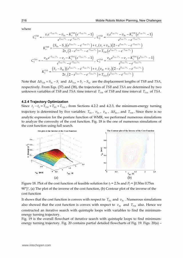
4.2.4 Trajectory Optimization
Since 0f TSB RS TSAt t T T T− = + + , from Sections 4.2.2 and 4.2.3, the minimum-energy turning
trajectory is determined by five variables: RST , Rsv , Rfv , Δ RSS , and TSBT . Since there is no
analytic expression for the posture function of WMR, we performed numerous simulations to analyze the convexity of the cost function. Fig. 18 is the one of numerous simulations of the cost function using full search.
0 0.5 1 1.5 2 2.5
0
0.2
0.4
0.6
0.8
1
TRS
[s]
vR
s [m
/s]
The Contour plot of the Inverse of the Cost Function
(a) (b)
Figure 18. Plot of the cost function of feasible solution for tf = 2.5s and Pf = [0.50m 0.75m
90°]T, (a) The plot of the inverse of the cost function, (b) Contour plot of the inverse of the
cost function
It shows that the cost function is convex with respect to RST and Rsv . Numerous simulations
also showed that the cost function is convex with respect to Rfv and TSBT also. Hence we
constructed an iterative search with quintuple loops with variables to find the minimum-energy turning trajectory. Fig. 19 is the overall flowchart of iterative search with quintuple loops to find minimum-energy turning trajectory. Fig. 20 contains partial detailed flowcharts of Fig. 19. Figs. 20(a) –
www.intechopen.com

Minimum-Energy Motion Planning for Differential-Driven Wheeled Mobile Robots
217
20(d) are iterative search loops to plan the trajectory of RS satisfying the feasibility
conditions of Eq. (36). In Fig. 20(d), maximum displacement length of RS is maxRS s fS L L= + as
shown in Fig. 15. Combining the solutions of minimum-energy trajectories for the required cornering motions, we can get the overall minimum-energy turning trajectory.
Figure 19. Overall flowchart of itertaive serach with quintuple loops to find minimum-energy turning trajectory
www.intechopen.com

Mobile Robots Motion Planning, New Challenges
218
No
Yes
No
Yes
Global
Optima
Exit
Given Ps, Pf, to, tf, zs, zf
= EBAT, TRSmin = 0, TRS
max = (tf – to)
TRS = (TRSmin + TRS
max)/2
= Find Local Optima for TRSRSE
TRSmin = TRS TRS
max = TRS
| |RS EE εΔ ≤
TRST = TRS – T
= Find Local Optima for TRSTT
RSEΔ
T
RS RS RSE E EΔΔ = −
0RSEΔ <
min
RSE
min
RS RSE E<
min
RS RSE E=
Yes
No
No
Yes
No
Yes
Local
Optima
= EBAT, vRsmin = vmin, vRs
max = vmax
vRs = (vRsmin + vRs
max)/2
vRsmin = vRs vRs
max = vRs
| |Rsv E
E εΔ ≤
vRsv = vRs v
= Find Local Optima for (TRS, vRsv)
Rs Rs Rs
v
v v vE E EΔΔ = −
0Rsv
EΔ <
= Find Local Optima for (TRS, vRs)RsvE
min
RsvE
min
Rs Rsv vE E<
min
Rs Rsv vE E=
Yes
No
Rs
v
vEΔ
| |Rfv E
E εΔ ≤
Rf Rf Rf
v
v v vE E EΔΔ = −
0Rfv
EΔ <
RfvE
min
RfvE
min
Rf Rfv vE E<
min
Rf Rfv vE E=
Rf
v
vEΔ
(a) (b) (c)
| |RSS E
E εΔ ≤
=RS RS RS
s
S S SE E EΔΔ −
0RSSEΔ <
min
RSSE
min
RS RSS SE E<
min
RS RSS SE E=
RSSE
RS
s
SEΔ
min
TSBE
min
TSB TSBE E=
TSBE
min
TSB TSBE E<
T
TSBEΔ
| |TSB EE εΔ ≤
= T
TSB TSB TSBE E EΔΔ −
0TSBEΔ <
(d) (e)
Figure 20. Partial flowchart of iterative serach with quintuple loops to find minimum-energy turning trajectory, (a) Search loop for finding TRS, (b) Search loop for finding vRs, (c) Search
loop for finding vRf, (d) Search loop for finding ΔSRS satisfying feasibility conditions of RS, Eq. (36), (e) Search loop for finding TTSB
4.3 Simulations and Experiments
4.3.1 Simulations A number of simulations were performed to evaluate the energy savings of the minimum-energy turning trajectory minimizing the cost function EW of Eq. (9) and compared to the trajectory using loss-minimization control, which optimizes the energy loss due to armature
resistance of the DC motor, RE .
www.intechopen.com

Minimum-Energy Motion Planning for Differential-Driven Wheeled Mobile Robots
219
Tables 5 and 6 show the simulations results for the variables of planned turning trajectory by the minimum-energy control and loss-minimization control, respectively. For a sufficient cruise motion in TSB and TSA, based on observation of the property of the minimum-energy
velocity profile shown in Fig. 5, we set the final time to tf = 15.0s greater than 20τv (≈ 7.8s).
Since there are many interations to find minimum-energy turning trajectory, we implemented the algorithm in C language and simulation takes much time about 4 ~ 6 hours for simulation constraints of Tables 5 and 6 using a PC with Intel Core2 Duo 2.13GHz processor.
Constraints Optimized Variables of Turning Trajectory
Pf D TRS vRs vRf ΔSRS TTSB TTSA ΔSTSB ΔSTSA EW
[(m) (m) (°)] (m) (s) (m/s) (m/s) (m) (s) (s) (m) (m) (J)
0.1 2.201 0.305 0.305 0.669 7.212 5.587 2.091 1.592 12.33 2.50 2.00 90
0.2 4.698 0.300 0.309 1.256 5.968 4.334 1.726 1.222 11.34
0.1 2.109 0.347 0.314 0.556 8.726 4.165 2.944 1.320 15.58 2.50 1.50 120
0.2 3.398 0.319 0.319 1.011 8.311 3.291 2.586 0.949 13.43
Table 5. Simluation results of minimum-energy turning trajectory
Constraints Optimized Variables of Turning Trajectory
Pf D TRS vRs vRf ΔSRS TTSB TTSA ΔSTSB ΔSTSA EW
[(m) (m) (°)] (m) (s) (m/s) (m/s) (m) (s) (s) (m) (m) (J)
0.1 2.703 0.323 0.319 0.747 6.736 5.562 2.050 1.552 12.87 2.50 2.00 90
0.2 3.724 0.370 0.348 1.384 6.310 4.966 1.652 1.168 12.21
0.1 2.607 0.319 0.309 0.616 7.854 4.539 2.915 1.286 16.46 2.50 1.50 120
0.2 3.223 0.381 0.338 1.115 7.873 3.904 2.516 0.910 14.23
Table 6. Simluation results of loss-minimization turning trajectory
The results of energy savings for various simulations are summarized in Table 7. It shows that the minimum-energy turning trajectory can save up to 8% of the energy drawn from the batteries compared with loss-minimization turning trajectory.
Pf D Total Energy Drawn from the Batteries
[(m) (m) (°)] (m) Minimum-Energy Loss-Minimization Energy Saving
0.1 12.33J 12.87J 4.38% 2.50 2.00 90
0.2 11.34J 12.21J 7.67%
0.1 15.58J 16.46J 5.65% 2.50 1.50 120
0.2 13.43J 14.23J 5.96%
Table 7. Comparison of energy savings of minimum-energy turning trajectory planning and loss-minimization turning trajectory planning
Fig. 21 shows a typical resultant trajectory that were performed for tf = 15.0s, Pf = [2.50m
1.50m 120°]T, and 0.2mD = . The mechanical time constant affects the velocity profiles of the
two optimization problems with different cost functions. Applying the Pontryagin’s Maximum Principle to optimize the cost function of loss-minimization control, we obtain
the mechanical time constants for loss-minimization control as follows: ( )1 2 /v vτ J J F= + for
translational motion and ( )1 2 /ω vτ J J F= − for rotational motion.
www.intechopen.com

Mobile Robots Motion Planning, New Challenges
220
0 5 10 150
0.2
0.4
0.6
0.8
Time [s]
Tra
nsl
ati
on
al
Vel
oci
ty [
m/s
]
0 5 10 150
0.5
1
Time [s]
Ro
tati
on
al
Vel
oci
ty [
m/s
]
Minimum-Energy
Loss-Minimization
Minimum-Energy
Loss-Minimization
0 0.5 1 1.5 2 2.5 3
-0.5
0
0.5
1
1.5
2
X-axis [m]
Y-a
xis
[m
]
Minimum-Energy
Loss-Minimization
(a) (b)
0 5 10 15-2
-1.5
-1
-0.5
0
0.5
1
1.5
2
Time [s]
Dra
wn
Ba
tter
y C
urr
ent
[A]
Minimum-Energy
Loss-Minimization
(c) (d)
0 5 10 150
5
10
15
Time [s]
To
tal
En
erg
y D
raw
n f
rom
Ba
tter
ies
[J]
Minimum-Energy
Loss-Minimization
0 5 10 15
-1
-0.5
0
0.5
1
1.5
2
Time [s]
Po
wer
Co
nsu
mp
tio
n [
Wa
tt]
Minimum-Energy
Loss-Minimization
(e) (f)
Figure 21. Simulations of minimum-energy control and loss-minimnization control turning
trajectory for tf = 15.0s, Pf = [2.50m 1.50m 120°]T, and D=0.2m, (a) Optimal velocity profile,
(b) Optimal planned path, (c) Armature current change, (d) Corresponding drawn battery current, (e) Comparison of energy consumption, (f) Corresponding power consumption
From Eq. (2), decreasing armature current increases the value of the back-emf and the motor speed. Because the mechanical time constants of minimum-energy control are less than those of loss-minimization control, the armature current in minimum-energy control quickly decreases during acceleration and deceleration, as shown in Fig. 21(d). Hence we can see that the minimum-energy control accelerates and decelerates more quickly than the loss-minimization control as shown in Fig. 21(a) and the minimum-energy control gives a cruise
www.intechopen.com
Minimum-Energy Motion Planning for Differential-Driven Wheeled Mobile Robots
221
or cruise-like motion to WMR in TSB and TSA as we expected. However, the loss-minimization control accelerates and decelerates in whole time since its mechanical time constant is much greater than that of minimum-energy control. Fig. 21(f) shows that although the minimum-energy control requires larger energy consumption than the loss-minimization control during acceleration, it consumes less energy after acceleration. Also note that during deceleration a certain amount of energy is regenerated and stored into the batteries in both minimum-energy control and loss-minimization control. However, amount of regenerated energy in the loss-minimization control is much smaller than that of the minimum-energy control since deceleration rate of loss-minimization control is much smaller than that of minimum-energy control due to larger mechanical time constants.
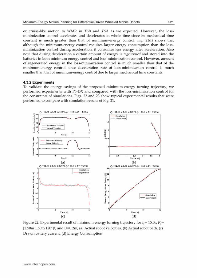
4.3.2 Experiments To validate the energy savings of the proposed minimum-energy turning trajectory, we performed experiments with P3-DX and compared with the loss-minimization control for the constraints of simulations. Figs. 22 and 23 show typical experimental results that were performed to compare with simulation results of Fig. 21.
0 5 10 150
0.1
0.2
0.3
0.4
Time [s]
Tra
nsl
ati
on
al
Vel
oci
ty [
m/s
]
Pf = [2.50 m 1.50 m 120 °], t
f = 15.0 s, D = 0.20 m
0 5 10 15-0.5
0
0.5
1
Time [s]
Rota
tion
al
Vel
oci
ty [
rad
/s]
Reference Velocity
Actual Velocity
Reference Velocity
Actual Velocity
0 0.5 1 1.5 2 2.5 3
0
0.5
1
1.5
X-axis [m]
Y-a
xis
[m
]
Pf = [2.50 m 1.50 m 120 °], t
f = 15.0 s, D = 0.20 m
Simulation
Experiment
(a) (b)
0 5 10 15-2
-1.5
-1
-0.5
0
0.5
1
1.5
2
Time [s]
Dra
wn
Cu
rren
t fr
om
Ba
tter
y [
A]
Pf = [2.50 m 1.50 m 120 °], t
f = 15.0 s, D = 0.20 m
Simulation
Experiment
0 5 10 15
0
2
4
6
8
10
12
14
Time [s]
Dra
wn
En
erg
y f
rom
Ba
tter
y [
J]
Pf = [2.50 m 1.50 m 120 °], t
f = 15.0 s, D = 0.20 m
Simulation
Experiment
(c) (d)
Figure 22. Experimental result of minimum-energy turning trajectory for tf = 15.0s, Pf =
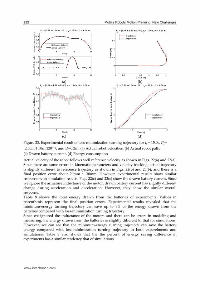
[2.50m 1.50m 120°]T, and D=0.2m, (a) Actual robot velocities, (b) Actual robot path, (c)
Drawn battery current, (d) Energy Consumption
www.intechopen.com
Mobile Robots Motion Planning, New Challenges
222
0 5 10 150
0.1
0.2
0.3
0.4
Time [s]
Tra
nsl
ati
on
al
Vel
oci
ty [
m/s
]
Pf = [2.50 m 1.50 m 120 °], t
f = 15.0 s, D = 0.20 m
0 5 10 15-0.5
0
0.5
1
Time [s]
Rota
tion
al
Vel
oci
ty [
rad
/s]
Reference Velocity
Actual Velocity
Reference Velocity
Actual Velocity
0 0.5 1 1.5 2 2.5 3
0
0.5
1
1.5
X-axis [m]
Y-a
xis
[m
]
Pf = [2.50 m 1.50 m 120 °], t
f = 15.0 s, D = 0.20 m
Simulation
Experiment
(a) (b)
0 5 10 15
-0.4
-0.2
0
0.2
0.4
0.6
Time [s]
Dra
wn
Cu
rren
t fr
om
Ba
tter
y [
A]
Pf = [2.50 m 1.50 m 120 °], t
f = 15.0 s, D = 0.20 m
Simulation
Experiment
0 5 10 15
0
5
10
15
Time [s]
Dra
wn
En
erg
y f
rom
Ba
tter
y [
J]
Pf = [2.50 m 1.50 m 120 °], t
f = 15.0 s, D = 0.20 m
Simulation
Experiment
(c) (d)
Figure 23. Experimental result of loss-minimization turning trajectory for tf = 15.0s, Pf =
[2.50m 1.50m 120°]T, and D=0.2m, (a) Actual robot velocities, (b) Actual robot path,
(c) Drawn battery current, (d) Energy consumption
Actual velocity of the robot follows well reference velocity as shown in Figs. 22(a) and 23(a). Since there are some errors in kinematic parameters and velocity tracking, actual trajectory is slightly different to reference trajectory as shown in Figs. 22(b) and 23(b), and there is a final position error about 20mm ~ 30mm. However, experimental results show similar response with simulation results. Figs. 22(c) and 23(c) show the drawn battery current. Since we ignore the armature inductance of the motor, drawn battery current has slightly different change during acceleration and deceleration. However, they show the similar overall response. Table 8 shows the total energy drawn from the batteries of experiments. Values in parenthesis represent the final position errors. Experimental results revealed that the minimum-energy turning trajectory can save up to 9% of the energy drawn from the batteries compared with loss-minimization turning trajectory. Since we ignored the inductance of the motors and there can be errors in modeling and measuring, the energy drawn from the batteries is slightly different to that for simulations. However, we can see that the minimum-energy turning trajectory can save the battery energy compared with loss-minimization turning trajectory in both expereiments and simulations. Table 8 also shows that the the percent of energy saving difference in experiments has a similar tendency that of simulations.
www.intechopen.com
Minimum-Energy Motion Planning for Differential-Driven Wheeled Mobile Robots
223
Pf D Total Energy Drawn from the Batteries
[(m) (m) (°)] (m) Minimum-Energy Loss-Minimization Energy Saving
0.1 12.05J (24mm) 13.10J (17mm) 8.71% 2.50 2.00 90
0.2 11.59J (23mm) 12.36J (24mm) 6.64%
0.1 15.34J (25mm) 16.71J (25mm) 8.93% 2.50 1.50 120
0.2 13.63J (25mm) 14.21J (31mm) 4.26%
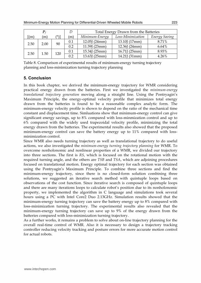
Table 8. Comparison of experimental results of minimum-energy turning trajectory planning and loss-minimization turning trajectory planning
5. Conclusion
In this book chapter, we derived the minimum-energy trajectory for WMR considering practical energy drawn from the batteries. First we investigated the minimum-energy translational trajectory generation moving along a straight line. Using the Pontryagin’s Maximum Principle, the energy-optimal velocity profile that minimizes total energy drawn from the batteries is found to be a reasonable complex analytic form. The minimum-energy velocity profile is shown to depend on the ratio of the mechanical time constant and displacement time. Simluations show that minimum-energy control can give significant energy savings, up to 8% compared with loss-minmization control and up to 6% compared with the widely used trapezoidal velocity profile, minimizing the total energy drawn from the batteries. The experimental results also showed that the proposed minimum-energy control can save the battery energy up to 11% compared with loss-minimization control. Since WMR also needs turning trajectory as well as translational trajectory to do useful actions, we also investigated the minimum-energy turning trajectory planning for WMR. To overcome nonholonomic and nonlinear properties of a WMR, we divided our trajectory into three sections. The first is RS, which is focused on the rotational motion with the required turning angle, and the others are TSB and TSA, which are adjoining procedures focused on translational motion. Energy optimal trajectory for each section was obtained using the Pontryagin’s Maximum Principle. To combine three sections and find the minimum-energy trajectory, since there is no closed-form solution combining three solutions, we suggested an iterative search method with quintuple loops based on observations of the cost function. Since iterative search is composed of quintuple loops and there are many iterations loops to calculate robot’s position due to its nonholonomic property, we implemented the algorithm in C language and simulations took several hours using a PC with Intel Core2 Duo 2.13GHz. Simulation results showed that the minimum-energy turning trajectory can save the battery energy up to 8% compared with loss-minimization turning trajectory. The experimental results also revealed that the minimum-energy turning trajectory can save up to 9% of the energy drawn from the batteries compared with loss-minimization turning trajectory. As a further works, it remains a problem to solve about on-line trajectory planning for the overall real-time control of WMR. Also it is necessary to design a trajectory tracking controller reducing velocity tracking and posture errors for more accurate motion control for actual robots.
www.intechopen.com

Mobile Robots Motion Planning, New Challenges
224
6. References
ActiveMedia Robotics. (2006). Pioneer 3 operations manual, Ver. 3 Alexander, J.C. & Maddocks, J.H. (1989). On the kinematics of wheeled mobile robots,
International Journal of Robotics Research, Vol. 8, No. 5, pp. 15-27, ISBN 0-387-97240-4 Angelo, C.D. ; Bossio, G. & Garcia, G. (1999). Loss minimization in DC motor drives,
Proceedings of the International Conference on Electric Machines and Drives, pp. 701-703, ISBN 0-7803-5293-9, Seattle, USA, May 1999
Aylett, R. (2002). Robots: Bringing intelligent machines to life, Barrons’s Educational Series Inc., ISBN 0-7641-5541-5, New York
Barili, A. ; Ceresa, M. & Parisi, C. (1995). Energy-saving motion control for an autonomous mobile robot, Proceedings of the IEEE International Symposium on Industrial Electronics, pp. 674-676, ISBN 0-7803-2683-0, Athens, Greece, Jul. 1995
Campion, G. ; d’Andrea-Novel, B. & Bastin, G. (1991). Modeling and state feedback control of nonholonomic mechanical systems, Proceedings of the IEEE International Conference on Decision and Control, pp. 1184-1189, Brighton, England, Dec. 1991
Campion, G. ; Bastin, G. & d’Andrea-Novel, B. (1996). Structural properties and classification of kinematic and dynamic models of wheeled mobile robots, IEEE Transactions on Robotics and Automation, Vol. 12, No. 1, pp. 47-62, ISSN 1042-296x
Choi, J.S. (2001). Trajectory planning and following for mobile robots with current and voltage constraints, Ph.D’s Thesis, KAIST, Daejeon, Korea.
Choset, H. ; Lynch, K.M. ; Hutchinson, S. ; Kantor, G. ; Burgard, W. ; Kavraki, L.E. & Thrun, S. (2005). Principles of robot motion, The MIT Press, ISBN 0-262-03327-5, Cambridge, MA
Divelbiss, A.W. & Wen, J. (1997). Trajectory tracking control of a car-trailer system, IEEE Transactions on Control Systems Technology, Vol. 5, No.3, pp. 269-278
Dubins, L.E. (1957). On curves of minimal length with a constraint on average curvature and with prescribed initial and terminal positions and tangents, American Journal of Mathematics, Vol. 79, No. 3, pp. 497-516
Egami, T. ; Morita, H. & Tsuchiya, T. (1990). Efficiency optimized model reference adaptive control system for a DC motor, IEEE Transactions on Industrial Electronics, Vol. 37, No. 1, pp. 28-33, ISSN 0278-0046
El-satter, A.A. ; Washsh, S. ; Zaki, A.M. & Amer, S.I. (1995). Efficiency-optimized speed control system for a separately-excited DC motor, Proceedings of the IEEE International Conference on Industrial Electronics, Control, and Instrumentation, pp. 417-422, Orlando, USA, Nov. 1995
Electro-Craft Corporation. (1977). DC motors, speed control, servo systems: An engineering handbook, Pergamon Press, ISBN 0-0802-1715-x, New York
Fiorini, P. & Shiller, Z. (1998). Motion planning in dynamic environments using velocity obstacles, International Journal of Robotics Research, Vol. 17, No. 7, pp. 760-772, ISSN 0278-3649
Jiang, J. ; Seneviratne, L.D. & Earles, S.W.E. (1996). Path planning for car-like robots using global analysis and local evaluation, Proceedings of the IEEE International Conference on Emerging Technologies and Factory Automation, Vol. 10, No. 5, pp. 577-593, ISBN 0-7803-3685-2, Kauai, USA, Nov. 1996
www.intechopen.com

Minimum-Energy Motion Planning for Differential-Driven Wheeled Mobile Robots
225
Kanayama, Y. & Miyake, N. (1985). Trajectory generation for mobile robots, Proceedings of the International Symposium of Robotics Research, pp. 333-340, ISBN 0-2620-6101-5, Gouvieux, France, Oct. 1985
Kanayama, Y. & Harman, B.I. (1989). Smooth local path planning for autonomous vehicles, Proceedings of the IEEE International Conference on Robotics and Automation, pp. 1265-1270, ISBN 0-8186-1938-4, Scottsdale, USA, May 1989
Kim, J. ; Yeom, H. ; Park, F.C. ; Park, Y.I. & Kim, Y. (2000). On the energy efficiency of CVT-based mobile robots, Proceedings of the IEEE International Conference on Robotics and Automation, pp. 1539-1544, ISBN 0-7803-5886-4, San Francisco, USA, Apr. 2000
Klein, J.T. ; Larsen, C. & Nichol, J. (2006). The design of the TransferBot: A robotic assistant for patient transfers and repositioning, International Journal of Assistive Robotics and Mechatronics, Vol. 7, No. 3, pp. 54-69, ISSN 1975-0153
Kusko, A. & Galler, D. (1983), Control means for minimization of losses in AC and DC motor drives, IEEE Transactions on Industrial Applications, Vol. 19, No. 4, pp. 561-570, ISSN 0885-8993
Kwok, S.T. & Lee, C.K. (1990). Optimal velocity profile design in incremental servo motor systems based on a digital signal processor, Proceedings of the Annual conference of the IEEE Industrial Electronics Society, pp. 262-266, ISBN 0-87942-600-4, Pacific Grove, USA, Nov. 1990
Laumond, J.P. ; Jacobs, P.E. & Murry, R.M. (1994). A motion planner for nonholonomic mobile robots, IEEE Transactions on Robotics and Automation, Vol. 10, No. 5, pp. 577-593, ISSN 1042-296x
Laumond, J.P. ; Nissoux, C. & Vendittelli, M. (1998). Obstacle distances and visibility for car-like robots moving forward, Proceedings of the IEEE International Conference on Robotics and Automation, pp. 33-39, ISBN 0-7803-4300-x, Leuven, Belgium, May 1998
Leonhard, W. (1996). Control of electrical drives, Springer-Verlag, ISBN 3-5405-9380-2, Berlin, Germany
Lineo, Inc. (2000). DIAPM RTAI Programming Guide 1.0, Italy Makimoto, T. & Sakai, Y. (2003). Evolution of low power electronics and its future
applications, Proceedings of the International Symposium on Low Power Electronics and Design, pp. 2-5, ISBN 1-58113-682-x, Seoul, Korea, Aug. 2003
Margaris, N. ; Goutal, T.; Doulgeri, Z. & Paschali, A. (1991). Loss minimization in DC drives, IEEE Transactions on Industrial Electronics, Vol. 38, No. 5, pp. 328-336
Mei, Y. ; Lu, Y.-H. ; Hu, Y.C. & Lee, C.S.G. (2004). Energy-efficient motion planning for mobile robots, Proceedings of the IEEE International Conference on Robotics and Automation, pp. 4344-4349, ISBN 0-7803-8232-3, New Orleans, USA, Apr. 2004
Mei, Y. ; Lu, Y.-H. ; Hu, Y.C. & Lee, C.S.G. (2005). Deployment strategy for mobile robots with energy and timing constraints, Proceedings of the IEEE International Conference on Robotics and Automation, pp. 2816-2821, ISBN 0-7803-8914-x, Barcelona, Spain, Apr. 2005
Mei, Y. ; Lu, Y.-H. ; Hu, Y.C. & Lee, C.S.G. (2006). Deployment of mobile robots with energy and timing constraints, IEEE Transactions on Robotics and Automation, Vol. 22, No. 3, pp. 507-522
Muir, P.F. & Neuman, C.P. (1987). Kinematic modeling of wheeled mobile robots, Journal of Robotic Systems, No. 2, pp. 281-329, ISSN 0741-2223
www.intechopen.com

Mobile Robots Motion Planning, New Challenges
226
Reeds, J.A. & Shepp, R.A. (1990). Optimal paths for a car that goes both forward and backward, Pacific Journal of Mathematics, Vol. 145, No. 2, pp. 367-393, ISSN 0030-8730
Rybski, P.E. ; Papankolopoulos, N.P. ; Stoeter, S.A. ; Krantz, D.G. ; Yesin, K.B. ; Gini, M. ; Voyles, R. ; Hougen, D.F. ; Nelson, B. & Erickson, M.D. (2000). Enlisting rangers and scouts for reconnaissance and surveillance, IEEE Robotics and Automation Magazine, Vol. 7, No. 4, pp. 14-24, ISSN 1070-9932
Sergaki, E.S. ; Stavrakakis, G.S. & Pouliezos, A.D. (2002). Optimal robot speed trajectory by minimization of the actuator motor electromechanical losses, Journal of Intelligent and Robotic Systems, Vol. 33, No. 2, pp. 187-207, ISSN 0921-0296
Spangelo, I. & Egeland, O. (1992). Generation of energy-optimal trajectories for an autonomous underwater vehicle, Proceedings of the IEEE International Conference on Robotics and Automation, pp. 2107-2112, ISBN 0-8186-2720-4, Nice, France, May 1992
Tal, J. (1973). The optimal design of incremental motion servo systems, Proceedings of the Annual Symposium on Incremental Motion Control Systems and Devices, , pp. 72-76, Urbana, USA
Trzynadlowski, A.M. (1988). Energy optimization of a certain class of incremental motion DC drives, IEEE Transactions on Industrial Electronics, Vol. 35, No. 1, pp. 60-66
Weigui, W. ; Huitang, C. & Peng-Yung, W. (1999). Optimal motion planning for a wheeled mobile robot, Proceedings of the IEEE International Conference on Robotics and Automation, pp. 41-46, ISBN 0-7803-5180-0, Detroit, USA, May 1999
Yun, X. and Yamamoto, Y. (1993). Internal dynamics of a wheeled mobile robot, Proceedings of the IEEE/RSJ International Conference on Intelligent Robots and Systems, Vol. 2, pp. 1288-1294, ISBN 0-7803-0823-9, Yokohama, Japan, Jul. 1993
Yun, X. (1995). State space representation of holonomic and nonholonomic constraints resulting from rolling contacts, Proceedings of the IEEE International Conference on Robotics and Automation, pp. 2690-2694, ISBN 0-7803-1965-6, Nagoya, Japan, May 1995
Yun, X. & Sarkar, N. (1998). Unified formulation of robotic systems with holonomic and nonholonomic constraints, IEEE Transactions on Robotics and Automation, Vol. 14, No. 4, pp. 640-650, ISSN 1042-296x
Zhang, G. ; Schmidhofer, A. & Schmid, A. (2003). Efficiency optimization at DC drives for small electrical vehicles, Proceedings of the IEEE International Conference on Industrial Technology, pp. 1150-1155, ISBN 0-7803-7852-0, Maribor, Slovenia, Dec. 2003
www.intechopen.com

Motion PlanningEdited by Xing-Jian Jing
ISBN 978-953-7619-01-5Hard cover, 598 pagesPublisher InTechPublished online 01, June, 2008Published in print edition June, 2008
InTech EuropeUniversity Campus STeP Ri Slavka Krautzeka 83/A 51000 Rijeka, Croatia Phone: +385 (51) 770 447 Fax: +385 (51) 686 166www.intechopen.com
InTech ChinaUnit 405, Office Block, Hotel Equatorial Shanghai No.65, Yan An Road (West), Shanghai, 200040, China
Phone: +86-21-62489820 Fax: +86-21-62489821
In this book, new results or developments from different research backgrounds and application fields are puttogether to provide a wide and useful viewpoint on these headed research problems mentioned above,focused on the motion planning problem of mobile ro-bots. These results cover a large range of the problemsthat are frequently encountered in the motion planning of mobile robots both in theoretical methods andpractical applications including obstacle avoidance methods, navigation and localization techniques,environmental modelling or map building methods, and vision signal processing etc. Different methods such aspotential fields, reactive behaviours, neural-fuzzy based methods, motion control methods and so on arestudied. Through this book and its references, the reader will definitely be able to get a thorough overview onthe current research results for this specific topic in robotics. The book is intended for the readers who areinterested and active in the field of robotics and especially for those who want to study and develop their ownmethods in motion/path planning or control for an intelligent robotic system.
How to referenceIn order to correctly reference this scholarly work, feel free to copy and paste the following:
Chong Hui Kim and Byung Kook Kim (2008). Minimum-Energy Motion Planning for Differential-Driven WheeledMobile Robots, Motion Planning, Xing-Jian Jing (Ed.), ISBN: 978-953-7619-01-5, InTech, Available from:http://www.intechopen.com/books/motion_planning/minimum-energy_motion_planning_for_differential-driven_wheeled_mobile_robots

© 2008 The Author(s). Licensee IntechOpen. This chapter is distributedunder the terms of the Creative Commons Attribution-NonCommercial-ShareAlike-3.0 License, which permits use, distribution and reproduction fornon-commercial purposes, provided the original is properly cited andderivative works building on this content are distributed under the samelicense.


