
METAL LEACHING FROM OIL SANDS FLUID PETROLEUM COKE
UNDER DIFFERENT GEOCHEMICAL CONDITIONS
A Thesis Submitted to the
College of Graduate and Postdoctoral Studies
In Partial Fulfillment of the Requirements
For the Degree of Master of Science
In the Department of Geological Sciences
University of Saskatchewan
Saskatoon
By
Mojtaba Abdolahnezhad
© Copyright Mojtaba Abdolahnezhad, November 2020. All rights reserved.
Unless otherwise noted, copyright of the material in this thesis belongs to the author

i
PERMISSION TO USE
In presenting this thesis in partial fulfillment of the requirements for a Postgraduate degree
from the University of Saskatchewan, I agree that the Libraries of this University may make it
freely available for inspection. I further agree that permission for copying of this thesis in any
manner, in whole or in part, for scholarly purposes may be granted by the professor or professors
who supervised my thesis work or, in their absence, by the Head of the Department or the Dean of
the College in which my thesis work was done. It is understood that any copying or publication or
use of this thesis or parts thereof for financial gain shall not be allowed without my written
permission. It is also understood that due recognition shall be given to me and to the University of
Saskatchewan in any scholarly use which may be made of any material in my thesis.
Requests for permission to copy or to make other uses of materials in this thesis/dissertation
in whole or part should be addressed to:
Head
Department of Geological Sciences
University of Saskatchewan
144 Geology Building, 114 Science Place
Saskatoon, SK, S7N 5E2
Canada
Dean
College of Graduate and Postdoctoral Studies
University of Saskatchewan
116 Thorvaldson Building, 110 Science Place
Saskatoon, SK, S7N 5C9
Canada
ii
ABSTRACT
The potential for metal leaching from fluid petroleum coke under different geochemical
conditions was investigated, with a specific focus on metal mobility. Oil sands mine closure
landscapes will contain overburden and upgrading by-products, including coke, stored
permanently under varied geochemical conditions, and previous field and laboratory studies show
that metal leaching is highly dependent upon the geochemical conditions within coke deposits.
Therefore, this research will identify the potential for metal leaching and the relationship with
water input composition with respect to the metal behavior. Petroleum coke contains elevated
solid-phase concentrations of V (1380 ± 45 mg kg−1), Ni (540 ± 18 mg kg−1), Mo (75.1 ± 3.5 mg
kg−1), and several other potentially hazardous metal(loid)s (e.g., Cu, Cr, Co, Se, Zn). Laboratory
column experiments focused on V, Ni, and Mo, which can occur at elevated dissolved
concentrations in coke deposits. Here, we examined metal leaching from fluid petroleum coke in
the presence of (i) meteoric water (pH = 7.2, Ionic strength < 0.01 M), (ii) oil sands process-
affected water (OSPW; pH = 8.6, I = 0.05 M), and (iii) acid rock drainage (ARD; pH = 2.0, I = 0.2
M). These solutions mimic water types that may interact with coke in closure landscapes. The
input, effluent, and profile samples collected over time showed that metal leaching is strongly
dependent upon input solution composition. Vanadium and Mo leaching were greatest with ARD
and OSPW, whereas sorption limited V and Mo mobility in the presence of meteoric water. Also,
Mo leaching was likely promoted by the high ionic strength of ARD and OSPW solutions due to
the release of weakly bound MoO42− ions via competitive desorption, and a shift to net positive
surface charge and dominance of H2MoO40 under ARD. Finally, enhanced Ni leaching in the
presence of meteoric water and ARD is due to the limited potential for sorption and to the enhanced
solubility of the hydroxide or carbonate phases. Although only a small proportion of total solid-
phase V, Ni, and Mo was released, our results demonstrated that geochemical conditions strongly
affect leaching behavior.

iii
ACKNOWLEDGEMENTS
I would first like to acknowledge the steady support and mentorship of my supervisor Dr.
Matthew Lindsay throughout my entire degree. Thank you for your patience and for providing
both academic and professional development opportunities throughout my time with group. Many
thanks to Dr. Samuel Butler for teaching me how to use the COMSOL Multiphysics simulation
software. Also, thank you to Dr. Jim Meriam for providing geophysical instruments used in this
research. Thank you to my external examiner for reviewing my thesis and providing comments.
My gratitude to Noel Galuschik for support in the lab, University of Saskatchewan staff Jing
Chen for completion of porewater analyses, and Rafael Gonzales for his help in operating
geophysical instruments and laboratory column setup.
Many thanks to my friends, especially Sana Daneshamouz, Alireza Zangouie, Soheil Naderi,
Mohsen Asadi, Arash Tavassoli, Reza Azinfar, Mohamed Narimani, Renaud Attioua, Rafael
Gonzales, and Mohamed Haiba for their motivation and friendship. Also, thank you for all the
soccer players in Hangry Hippos and Due Birra Unito team for the joy and happiness throughout
my program. Special thanks for Tod LeBlanc for managing the soccer team and inspiring me with
geophysical inversion codes. Also, thanks for Lindsay group members for nominated me as the
keeper of time, social butterfly, best office playlist, and jack of all trades’ awards at our annual
holiday parties.
Words cannot express my gratitude for having such a supportive brother through my
academic and life, thank you so much. Finally, a special thank you to my parents, Zahra and
Ardeshir, for their love and for supporting my decision to move so far away to pursue my dream
especially my Mom, Zahra, as she was my first teacher. She taught me to be an independent,
strong, and passionate person about my career. I remember this poem by Iranian poet Ferdowsi:
“Those who have knowledge, art, and culture,why worry if they lack treasure?”
I dedicate this thesis with a Persian poem by Saadi Shirazi to all health workers around the
globe who are brave enough to stay in frontline against COVID-19.
"Human beings are members of a whole, since in their creation they are of one essence.
When the conditions of the time brings a member (limb) to pain,

iv
the other members (limbs) will suffer from discomfort.
You, who are indifferent to the misery of others,
it is not fitting that they should call you a human being."

v
TABLE OF CONTENTS
PERMISSION TO USE ................................................................................................................. i
ABSTRACT ................................................................................................................................... ii
ACKNOWLEDGEMENTS ........................................................................................................ iii
TABLE OF CONTENTS ............................................................................................................. v
LIST OF TABLES ..................................................................................................................... viii
LIST OF FIGURES ................................................................................................................... viii
LIST OF ABBREVIATIONS ................................................................................................... xiii
CHAPTER 1: INTRODUCTION ................................................................................................ 1
1.1. Research Hypothesis and Objectives ................................................................................. 2
CHAPTER 2: LITERATURE REVIEW ................................................................................... 3
2.1. Alberta Oil Sands ................................................................................................................ 3
2.2. Bitumen Extraction ............................................................................................................. 4
2.3. Bitumen Upgrading ............................................................................................................. 5
2.4. Petroleum Coke ................................................................................................................... 6
2.4.1. Physical Properties .................................................................................................... 6
2.4.2. Chemical Composition .............................................................................................. 8
2.5. Metal Geochemistry ............................................................................................................ 9
2.5.1. Vanadium ................................................................................................................... 9
2.5.2. Nickel ........................................................................................................................ 12
2.5.3. Molybdenum ............................................................................................................ 15
2.6. Mine Closure Considerations ........................................................................................... 18
2.7. Hydrogeophysics ................................................................................................................ 19
CHAPTER 3: MATERIALS AND METHODS ...................................................................... 20
vi
3.1. Laboratory Columns Experiments .................................................................................. 20
3.1.1. Small Column Setup ................................................................................................ 20
3.1.2. Large Column Setup ............................................................................................... 21
3.1.3. Input Solutions ......................................................................................................... 23
3.2. Aqueous-Phase Analyses ................................................................................................... 24
3.3. Solid-Phase Analyses ......................................................................................................... 25
3.3.1. Specific Surface Area Analyses .............................................................................. 25
3.3.2. Particle Size Distribution ........................................................................................ 26
3.3.3. Electron Microscopy ............................................................................................... 26
3.3.4. Cation Exchange Capacity Analysis ...................................................................... 26
3.3.5. pH Point of Zero Charge ........................................................................................ 26
3.3.6. Elemental Analyses .................................................................................................. 27
3.4. Data Analysis ..................................................................................................................... 27
3.4.1. Statistical Methods .................................................................................................. 27
3.4.2. Transport Parameters ............................................................................................. 28
3.4.3. Geochemical Modelling ........................................................................................... 29
3.4.4. Geophysical Modeling ............................................................................................. 29
3.4.5. Cumulative Mass Release Calculations ................................................................. 31
CHAPTER 4: RESULTS AND DISCUSSION ........................................................................ 32
4.1. Physical Characteristics .................................................................................................... 32
4.2. Chemical Characteristics .................................................................................................. 34
4.3. Small Columns ................................................................................................................... 38
4.3.1. Aqueous Geochemistry ........................................................................................... 38
4.3.2. Transport Parameters ............................................................................................. 49
4.4. Large Column .................................................................................................................... 51
4.4.1. Aqueous Geochemistry ........................................................................................... 51
4.4.2. Geophysical inversion and forward modeling results .......................................... 60
4.4.3. Transport properties ............................................................................................... 63
CHAPTER 5: CONCLUSIONS ................................................................................................ 65
REFERENCES ............................................................................................................................ 67
vii
APPENDIX A: FORWARD AND INVERSE GEOPHYSICAL MODELING .................... 79
APPENDIX B: MASS PACKED INSIDE COLUMNS ........................................................... 81
APPENDIX C: CATION EXCHANGE CAPACITY ............................................................. 82
APPENDIX D: VANADIUM (V) REACTIONS AND FORMATION CONSTANT .......... 86
APPENDIX E: PH POINT OF ZERO CHARGE ................................................................... 87
APPENDIX F: BULK ELEMENTAL ANALYSES .............................................................. 101
APPENDIX G: AQUEOUS GEOCHEMISTRY DATA FOR COLUMNS ........................ 113
APPENDIX H: CUMULATIVE MASS RELEASE .............................................................. 186
APPENDIX I: BREAKTHROUGH CURVE ......................................................................... 188

viii
LIST OF TABLES
Table 3.1. Target input solution composition for DI, synthetic OSPW (OSPWa), field OSPW
(OSPWb), and ARD. ..................................................................................................................... 24
Table 4.1. Physical properties of acid-washed sand (AWS) and coke. ........................................ 32
Table 4.2. Summary of selected elemental contents for fluid petroleum coke samples collected
from coker units and field deposits. .............................................................................................. 36
Table 4.3. Cumulative mass release per kg of fluid petroleum coke for the small columns. ...... 44
Table 4.4. Calculated hydraulic parameters for dry coke during DI input. .................................. 50
Table 4.5. Average linear velocity for the large column, measured based on mid-point theory for
the first tracer test including injection and decay. ........................................................................ 61
Table 4.6. Calculated hydraulic parameters for the large column including first tracer test injection
part (A1), decay part (A2), and second tracer test-decay part (B2). ............................................. 64

ix
LIST OF FIGURES
Figure 2.1. Map of Alberta oil sands regions (AOSR). ................................................................. 4
Figure 2.2. Schematic diagram of a fluid coker (after Gray, 2015). .............................................. 6
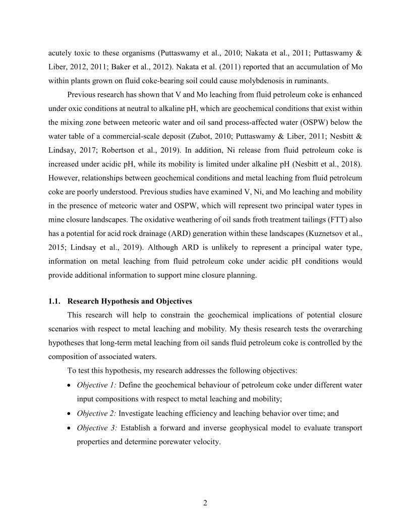
Figure 2.3. Scanning electron microscopy (SEM) image of fluid petroleum coke. ...................... 7
Figure 2.4. Backscattered electron (BSE) image of coke particle thin sections, showing the interior
of coke particles. ............................................................................................................................. 7
Figure 2.5. Chemical structures of metal species (Ni and V) in bitumen (after Gray, 2015). ....... 8
Figure 2.6. Pourbaix (Eh–pH) diagram for a total aqueous concentration of 1 μM vanadium. .. 11
Figure 2.7. Predominance diagram showing aqueous V(V) speciation as a function of pH and
[V]T. .............................................................................................................................................. 12
Figure 2.8. Pourbaix (Eh–pH) diagram for Ni at 0.9 μM total aqueous concentration. .............. 14
Figure 2.9. Nickel(II) hydroxide speciation (top), Ni(II) complexation in the presence of sulfate
(1000 mg kg─1; middle), and Ni(II) complexation in open carbonate systems (bottom). ............ 15
Figure 2.10. Pourbaix (Eh–pH) diagram for a median concentration of Mo at 1 μM total aqueous
concentration found within fluid petroleum coke deposits. .......................................................... 17
Figure 2.11. Predominance diagram showing aqueous Mo(VI) speciation as a function of pH and
[Mo]T. ............................................................................................................................................ 17
Figure 3.1. Schematic diagram and photo of the small column experiments. The coke layers were
placed between two acid washed sand (AWS) layers. .................................................................. 21
Figure 3.2. Graphical representation of the placement of platinum wire (left); schematic
representation of column experiment (middle); photograph of the fully constructed column (right).
....................................................................................................................................................... 22
Figure 4.1. Scanning electron microprobe (SEM) images of fluid petroleum coke; (a) dry coke,
(b) slurry coke, (c, d) dry coke, and (e, f) slurry coke. ................................................................. 33
Figure 4.2. Bulk elemental analyses for elements in fluid petroleum coke. Box lines define 25th,
50th, and 75th percentiles; lower and upper whiskers define 10th and 90th percentiles. ................. 35
Figure 4.3. Top: Backscattered electron (BSE) images of fluid coke particles in thin section.
Yellow dots and labels denote the energy dispersive X-ray (EDX) spectra for sample A (top) and
sample D (bottom). Yellow dots indicate locations of the obtained spectra while the points without
a red dot spectra was obtained for that specific mineral. .............................................................. 37

x
Figure 4.4. Influent (open symbol) and effluent (filled symbols) pH, electrical conductivity (EC),
and alkalinity as a function of pore volume (PV) for the small columns experiment during
deionized (DI), oil sand processing affected water (OSPW), and acid rock drainage (ARD)
solutions. The orange triangles and blue squares represent dry coke and slurry coke, respectively.
Units for alkalinity are mg L−1 as CaCO3 and values plotted on the x-axis are equal to zero. ..... 39
Figure 4.5. Influent (open symbol) and effluent (filled symbols) dissolved concentration of S and
Fe as a function of pore volume (PV) for the small columns experiment during deionized (DI) and
oil sand processing affected water (OSPW) solutions. The orange triangles and blue squares
represent dry and slurry coke, respectively. Values plotted on the x-axis are equal to zero. ....... 40
Figure 4.6. Influent (open symbol) and effluent (filled symbols) dissolved concentration of V, Mo,
and Ni for the small columns under deionized (DI), oil sand processing affected water (OSPW),
and acid rock drainage (ARD) as a function of pore volume (PV). Orange triangles and blue
squares represent dry and slurry coke, respectively. Data on the x-axis are below the method
detection limit and are assumed to be zero. .................................................................................. 42
Figure 4.7. Pourbaix (Eh–pH) diagram for vanadium (top) and a predominance diagram showing
aqueous V(V) speciation as a function of pH and total V concentration (bottom). All V aqueous
species were assumed to be V(V) in the second figure. Squares, triangles, and circles represent
data points for deionized (DI), oil sand processing affected water (OSPW), and acid rock drainage
(ARD), respectively. Filled symbols represent slurry coke and empty symbols represent dry coke.
....................................................................................................................................................... 43
Figure 4.8. Cumulative mass release per kg of coke under deionized (DI), oil sand processing
affected water (OSPW), and acid rock drainage (ARD) as function of pore volume (PV). Orange
lines represent the dry coke; blue lines represent slurry coke. ..................................................... 45
Figure 4.9. Pourbaix (Eh–pH) diagram for Ni. Squares, triangles, and circles represent data points
for deionized (DI), oil sand processing affected water (OSPW), and acid rock drainage (ARD),
respectively. Filled symbols represent data points for slurry coke and blank symbols represent dry
coke. .............................................................................................................................................. 46
Figure 4.10. Pourbaix (Eh–pH) diagram (top) and Log concentration vs. pH for Mo(VI) (bottom).
Squares, triangles, and circles represent data points for deionized (DI), oil sand processing affected
water (OSPW), and acid rock drainage (ARD), respectively. Filled symbols represent data points
for slurry coke; blank symbols represent data points for dry coke. .............................................. 48
Figure 4.11. Breakthrough curve for dry coke during DI input (black line). Error bars represent
the electrode ±2.5% electrode sensitivity. Red dashed lines indicate the lower and higher 95%
confidence. .................................................................................................................................... 50
Figure 4.12. Influent (open symbols) and effluent (filled symbols) pH, EC, and alkalinity as a
function of pore volume (PV) for the large column experiment during deionized (DI), oil sand
processing affected water (OSPW), and acid rock drainage (ARD). The units for alkalinity are mg
L−1 as CaCO3 and values plotted on the x-axis are equal to zero. Vertical dashed lines indicate
transitions between input solution compositions. The vertical black dotted line during OSPW input
xi
indicates the transition from synthetic to field OSPW. Hatched areas represent times during which
tracer tests were conducted. .......................................................................................................... 52
Figure 4.13. Influent (open symbols) and effluent (filled symbols) S and Fe concentrations as a
function of pore volume (PV) for the large column experiment during deionized (DI), oil sand
processing affected water (OSPW), and acid rock drainage (ARD). Vertical dashed lines indicate
transitions between input solution compositions. Vertical black dotted line during OSPW input
indicates the transition from synthetic to field OSPW. Hatched areas represent times during which
tracer tests were conducted. .......................................................................................................... 53
Figure 4.14. Influent (open symbols) and effluent (filled symbols) V, Mo, and Ni aqueous
concentrations as a function of pore volume for the large column experiment during deionized
(DI), oil sand processing affected water (OSPW), and acid rock drainage (ARD). All
concentrations are in μg L−1 and values plotted on x-axis are below the method detection limit.
Vertical dashed lines indicate a transition between input solution compositions. Vertical black
dotted line in the OSPW phase indicates the transition from synthetic to field OSPW. Hatched
areas represent times during which tracer tests were conducted. ................................................. 54
Figure 4.15. Pourbaix (Eh–pH) diagram for vanadium (top) and predominance diagram showing
aqueous V(V) speciation as a function of pH and total V concentration (bottom). Blue squares, red
triangles, and orange circles represent data points for during deionized (DI), oil sand processing
affected water (OSPW), and acid rock drainage (ARD), respectively. ........................................ 55
Figure 4.16. Cumulative V, Ni, and Mo release from fluid petroleum coke under sequential input
of different water compositions including deionized (DI), oil sand processing affected water
(OSPW), and acid rock drainage (ARD) for the large column. All units are in μg L−1. .............. 56
Figure 4.17. Pourbaix (Eh–pH) diagram for Ni. Blue squares, red triangles, and orange circles
represent data points for deionized (DI), oil sand processing affected water (OSPW), and acid rock
drainage (ARD), respectively. ...................................................................................................... 57
Figure 4.18. Pourbaix (Eh–pH) diagram for vanadium (top) and predominance diagram showing
Mo(VI) aqueous speciation as function of pH and concentration (bottom). Blue squares, red
triangles, and orange circles represent data points for deionized (DI), oil sand processing affected
water (OSPW), and acid rock drainage (ARD), respectively. ...................................................... 59
Figure 4.19. Apparent resistivity as function of time (left) and linear regression of mid-point
(right) which define the average linear velocity for the first tracer. This includes the injection of
the tracer (top) and decay of the first tracer (bottom). Electrodes were configured in a ring position,
with R1 to R8 placed from the bottom to top of the column. ....................................................... 61
Figure 4.20. Forward modeling results for the first four rings (apparent resistivity vs. time) during
the first tracer test. The black line is the measured apparent resistivity associated with the ring
positions. Red, blue, and orange lines are the calculated apparent resistivity for that specific level
±2.5 cm. ........................................................................................................................................ 62
Figure 4.21. Forward modeling results for the first four rings (apparent resistivity vs. time) during
the first tracer test (Decay). The black line is the measured apparent resistivity associated with the

xii
ring positions. Red, blue, and orange lines are the calculated apparent resistivity for that specific
level ±2.5 cm. ................................................................................................................................ 63
Figure 4.22. Breakthrough curve for the large column as a function of time (black line). Error bars
represent the electrode ±2.5% electrode sensitivity. Red dashed lines indicate the lower and higher
95% confidence. ............................................................................................................................ 64

xiii
LIST OF ABBREVIATIONS
AOSR Athabasca oil sand region
ARD Acid rock drainage
AWS Acid washed sand
CBE Charge balance error
CEC Cation exchange capacity
CFT Centrifuged fine tailing
CSS Cycling steam stimulation
DI Deionized water
EC Electrical conductivity
EDX Energy dispersive X-ray
EMPA Electron microprobe analyses
ER Electrical resistivity
FTT Froth treatment tailings
HDPE High-density polyethylene
IC Ion chromatography
ICP-MS Inductively coupled plasma–mass spectrometry
ICP-OES Inductively coupled plasma–optical emission spectroscopy
MLSB Mildred lake settling basin
OSPW Oil sand process-affected water
PES polyethersulfone
pHPZC pH point of zero charge
PP Polypropylene
PSD Particle size distributions
PTFE Polyfluorotetraethylene
PV Pore volume
SAGD Steam assisted gravity drainage
SCO Synthetic crude oil

xiv
SEM Scanning electron microscopy
SP Self potential
SSA Specific surface area
XANES X-ray absorption near edge structure

1
CHAPTER 1: INTRODUCTION
Oil sand deposits in northern Alberta, Canada contain a mixture of bitumen, mineral solids,
and water (Liu et al., 2005). Bitumen is extracted from deposits in the Athabasca Oil Sands Region
(AOSR) either by (i) surface mining, hot water addition, and gravity separation or (ii) in situ
heating and pumping followed by water removal (AER, 2019). Extracted bitumen is highly viscous
and contains high asphaltene and sulfur contents, entrained solids and water, and elevated metal
and salt contents (Gray, 2015). These characteristics make extracted bitumen unsuitable for simple
refineries and instead bitumen is shipped to high conversion refineries. Many oil sands operations
in the AOSR upgrade extracted bitumen to synthetic crude oil (SCO), which can be sold to
conventional refineries at higher prices.
Bitumen upgrading involves several processes including vacuum distillation, coking, and
hydro-conversion. Coking involves the thermal cracking of long-chain hydrocarbons in the non-
distillable bitumen fraction into light hydrocarbons including naphtha, kerosene, and gas oils.
Petroleum coke, the principal by-product of the coking process, was generated approximately 170
kg for m3 of SCO in 2019 (AER, 2019). Fluid coking and delayed coking are the two principal
coking methods used in the AOSR. The resulting fluid petroleum coke and delayed petroleum coke
exhibit different physical and chemical properties, with the former accounting for approximately
60% of current petroleum coke production (AER, 2019). Approximately 1.13 × 10⁷ t of petroleum
coke were generated during bitumen upgrading in 2019 (AER, 2019). Coke stockpiles in the
AOSR have steadily increased over time and reached 1.32 × 10⁸ t by the end of 2019 (AER, 2019).
These coke stockpiles will be integrated into mine closure landscapes in the AOSR (Simhayov et
al., 2017), where the disturbed footprint due to surface mining activities currently exceeds 990 km2
(CAPP, 2018).
Petroleum coke is a low-density carbonaceous material that contains a wide range of major,
minor and trace elements (Kessler & Hendry, 2006; Zubot et al., 2012; Nesbitt et al., 2017).
Elevated metal concentrations in petroleum coke leachate are a potential risk to water quality in
mine closure landscapes that contain petroleum coke (Zubot et al., 2012; Nesbitt & Lindsay, 2017;
Nesbitt et al., 2018, 2017; Robertson et al., 2019). Elevated V and Ni in coke-associated leachates
can accumulate within plants and invertebrates in the AOSR, and these leachates are generally
2
acutely toxic to these organisms (Puttaswamy et al., 2010; Nakata et al., 2011; Puttaswamy &
Liber, 2012, 2011; Baker et al., 2012). Nakata et al. (2011) reported that an accumulation of Mo
within plants grown on fluid coke-bearing soil could cause molybdenosis in ruminants.
Previous research has shown that V and Mo leaching from fluid petroleum coke is enhanced
under oxic conditions at neutral to alkaline pH, which are geochemical conditions that exist within
the mixing zone between meteoric water and oil sand process-affected water (OSPW) below the
water table of a commercial-scale deposit (Zubot, 2010; Puttaswamy & Liber, 2011; Nesbitt &
Lindsay, 2017; Robertson et al., 2019). In addition, Ni release from fluid petroleum coke is
increased under acidic pH, while its mobility is limited under alkaline pH (Nesbitt et al., 2018).
However, relationships between geochemical conditions and metal leaching from fluid petroleum
coke are poorly understood. Previous studies have examined V, Ni, and Mo leaching and mobility
in the presence of meteoric water and OSPW, which will represent two principal water types in
mine closure landscapes. The oxidative weathering of oil sands froth treatment tailings (FTT) also
has a potential for acid rock drainage (ARD) generation within these landscapes (Kuznetsov et al.,
2015; Lindsay et al., 2019). Although ARD is unlikely to represent a principal water type,
information on metal leaching from fluid petroleum coke under acidic pH conditions would
provide additional information to support mine closure planning.
1.1. Research Hypothesis and Objectives
This research will help to constrain the geochemical implications of potential closure
scenarios with respect to metal leaching and mobility. My thesis research tests the overarching
hypotheses that long-term metal leaching from oil sands fluid petroleum coke is controlled by the
composition of associated waters.
To test this hypothesis, my research addresses the following objectives:
Objective 1: Define the geochemical behaviour of petroleum coke under different water
input compositions with respect to metal leaching and mobility;
Objective 2: Investigate leaching efficiency and leaching behavior over time; and
Objective 3: Establish a forward and inverse geophysical model to evaluate transport
properties and determine porewater velocity.

3
CHAPTER 2: LITERATURE REVIEW
This chapter provides a review of bitumen extraction and upgrading, and establishes the
current state of knowledge of the physical and chemical characteristics of oil sands petroleum coke.
The environmental geochemistry of vanadium, nickel, and molybdenum are reviewed, and
geophysical techniques and modeling approaches are described.
2.1. Alberta Oil Sands
Oil sands deposits in northern Alberta, Canada represent the largest crude bitumen reserve and
the third-largest proven oil reserve in the world (AER, 2015). These deposits have in-place bitumen
reserves estimated at 293.1 billion m3 (AER, 2015), divided among three deposits: Athabasca, Cold
Lake, and Peace River (Figure 2.1). The Athabasca deposit, also known as the AOSR, is the largest
of these three deposits with recoverable bitumen reserves estimated 171 billion barrels (CAPP,
2018).
The AOSR consists of three main formations: the deeper Waterways, Wabiskaw-McMurray,
and Clearwater (Hein & Cotterill, 2006; Gibson et al., 2013). All of these formations are overlain
by a thin layer of Quaternary age glacial till sediment (Gibson et al., 2013). The near surface
Clearwater Formation, which represent an approximately 10 m of shale unit, grades from silt to fine-
grained sand downward, covering the Wabiskaw-McMurray Formation (Gibson et al., 2013).
Bitumen in the AOSR hosted within the Wabiskaw-McMurray Formation was deposited during the
Cretaceous period (145.5–65.5 Ma) and consists of sand with interbedded shales, sands, and silts
(Hein & Cotterill, 2006; Gibson et al., 2013). The deeper Waterways Formation of Devonian age
underlies the Wabiskaw-McMurray Formation and contains evaporite deposits within carbonate
rock (Gibson et al., 2013).
The oil sands in the AOSR comprise silt, clay, sand, water, and bitumen. Oil sand ore, by
weight, contains approximately 85% mineral solids, 5% water, and 10% bitumen (Liu et al., 2005;
Zubot et al., 2012). The mineral solids contain abundant clays, including kaolinite (40–70% [w/w]),
illite (28–45% [w/w]), and montmorillonite (1–15% [w/w]) and are dominated by quartz
(Chalaturnyk et al., 2002).

4
Bituminous ore within the AOSR occurs in the southwest dipping McMurray formation, which
outcrops near Fort McMurray, Alberta along the Athabasca and Clearwater rivers. Bitumen is a high
molecular weight, viscous hydrocarbon that needs further upgrading before it can be sent for
distribution (Masliyah et al., 2004; Liu et al., 2005).
Figure 2.1. Map of Alberta oil sands regions (AOSR). Public domain image created by N.
Einstein (2011), Athabasca Oil Sands Mining Map,
https://commons.wikimedia.org/wiki/File:Athabasca_Oil_Sands_map.png.
2.2. Bitumen Extraction
Oil sands operations in the AOSR extract bitumen using two main approaches: in situ
extraction or surface mining. In situ bitumen extraction by steam assisted gravity drainage (SAGD)
or cycling steam stimulation (CSS) target oil sands positioned approximately 150 to 450 m below
the ground surface. In contrast, surface mining methods are suitable for oil sands located within
80 m of the ground surface (Kasperski & Mikula, 2011). Consequently, approximately 20% of
bitumen reserves in the AOSR are extracted by surface mining operations (CAPP, 2018). These

5
operations use large power shovels and dump trucks to mine and haul oil sands ore to preparation
plants. Mined ore is crushed and screened before being sent by conveyors to a slurry preparation
plant, where hot water and process aids (e.g., sodium hydroxide, sodium citrate) are added to
enhance bitumen extraction (Chalaturnyk et al., 2002; Masliyah et al., 2004). The bitumen slurry is
pumped to an extraction plant via hydrotransport pipelines, where liberated bitumen attaches to
entrained air bubbles to produce bitumen froth (Liu et al., 2005). The conditioned bitumen slurry
then enters large gravity separation vessels, where the buoyant bitumen froth separates from
liberated solids. The coarse solids are hydrotransported to tailings ponds whereas finer-grained
solids (i.e., middlings), containing up to 4% (w/w) bitumen, are retained for additional extraction.
The recovered bitumen froth is deaerated and sent to froth treatment, where diluent hydrocarbons
(i.e., naphtha, paraffins) are added to decrease bitumen viscosity and liberate entrained solids
(Masliyah et al., 2004; Liu et al., 2005). Following solvent recovery, the liberated solids are
hydrotransported to tailings ponds and the extracted bitumen is retained for further processing.
Overall bitumen recovery during the extraction process typically ranges from 88 to 95%
(Chalaturnyk et al., 2002; Masliyah et al., 2004; Liu et al., 2005).
2.3. Bitumen Upgrading
Extracted bitumen cannot be processed at conventional refineries due the presence of water,
solids, and impurities (e.g., sulfur, nitrogen, metals), high asphaltene content, and a low hydrogen
to carbon ratio. Consequently, approximately 40% of all extracted bitumen is upgraded to SCO,
which can be processed at conventional refineries and sells at a premium over extracted bitumen.
Bitumen upgrading to SCO involves the coking process, which involves thermal cracking of
long and heavy chain hydrocarbons to shorter and lighter hydrocarbon compounds. In the AOSR,
upgrading processes use either fluid or delayed coking, producing fluid or delayed petroleum coke,
respectively (Gray, 2015). These methods involve the use of high temperature (350–550 °C,
depending on the coking method) to break down long-chain hydrocarbons within the bitumen (Gray,
2015). The two types of petroleum coke have different physical and chemical properties depending
on the bitumen feed and coking method (Kessler & Hendry, 2006).
In fluid coking units, bitumen is sprayed into the reactor while steam is injected from the
bottom and coats the hot coke particles. Thermal cracking occurs on the surface of these particles at
a temperature of 510–550 °C (Figure 2.2). Long and complex molecules crack into lighter and
shorter hydrocarbons and leave the reactor vessels from the top as a vapor phase, moving to a

6
fractionator where vapor is fractioned into various petroleum products like gases, naphtha, light gas
oil, and heavy gas oil. The coke particles in this process tend to grow in size; therefore, fine particles
are separated by elutriation (based on size, shape, and density), and these relatively cold coke
particles pass to the burner where they are combusted with air to supply heat to the reactor. Excess
petroleum coke is removed from the burner vessel, mixed with OSPW to form a slurry, and
hydrotransported by pipeline to dedicated deposits within tailings impoundments (Gray, 2015).
Figure 2.2. Schematic diagram of a fluid coker (after Gray, 2015).
2.4. Petroleum Coke
Petroleum coke is a by-product of the coking process, and is generated at a rate of over
170 kg for m3 of SCO (AER, 2019). The bitumen upgrading process resulted in the production of
approximately 1.13 × 10⁷ t of petroleum coke, and coke stockpiles in the AOSR have steadily
increased over time, reaching 1.32 × 10⁸ t by the end of 2019 (AER, 2019). Over the lifetime of oil
sands operations, coke stockpiled is expected to reach nearly 1 billion m3 (Fedorak & Coy, 2006).
2.4.1. Physical Properties
Fluid petroleum coke consists of uniform spherical particles with a relatively low particle
density (1.61 g cm−3) and a fine sandy texture (Figure 2.3), resulting in a high hydraulic permeability
of 1.48 ± 0.12 × 10⁻⁵ m s−1, measured by Zubot (2010).
7
Figure 2.3. Scanning electron microscopy (SEM) image of fluid petroleum coke.
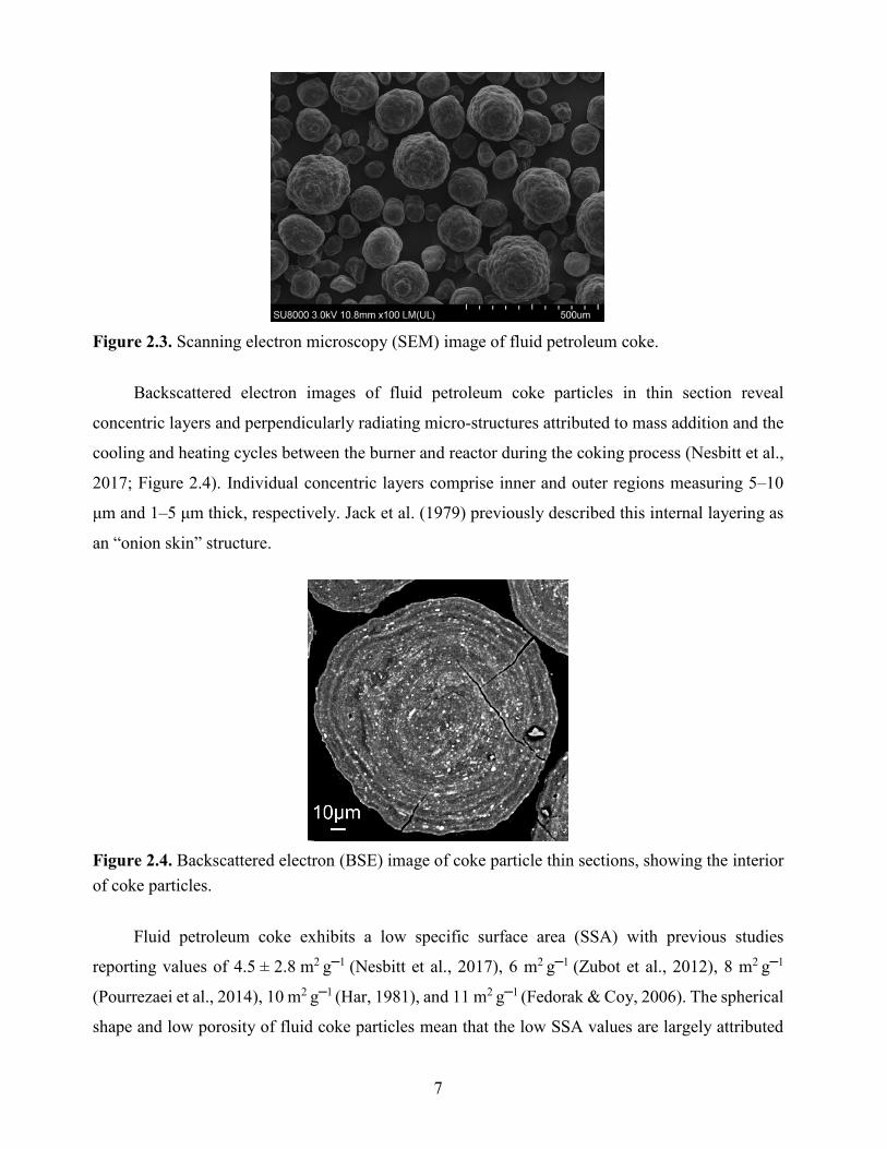
Backscattered electron images of fluid petroleum coke particles in thin section reveal
concentric layers and perpendicularly radiating micro-structures attributed to mass addition and the
cooling and heating cycles between the burner and reactor during the coking process (Nesbitt et al.,
2017; Figure 2.4). Individual concentric layers comprise inner and outer regions measuring 5–10
μm and 1–5 μm thick, respectively. Jack et al. (1979) previously described this internal layering as
an “onion skin” structure.
Figure 2.4. Backscattered electron (BSE) image of coke particle thin sections, showing the interior
of coke particles.
Fluid petroleum coke exhibits a low specific surface area (SSA) with previous studies
reporting values of 4.5 ± 2.8 m2 g
─1 (Nesbitt et al., 2017), 6 m2
g─1
(Zubot et al., 2012), 8 m2 g
─1
(Pourrezaei et al., 2014), 10 m2 g
─1 (Har, 1981), and 11 m2
g─1
(Fedorak & Coy, 2006). The spherical
shape and low porosity of fluid coke particles mean that the low SSA values are largely attributed

8
to primary surfaces. These physical properties also explain why fluid petroleum coke exhibits much
lower porosity than activated carbon (>750 m2 g─1). Nevertheless, Pourrezaei et al. (2014) reported
that mesopores with 2–40 nm apertures are likely important for geochemical reactions at surfaces of
fluid petroleum coke particles.
2.4.2. Chemical Composition
Fluid petroleum coke is a low density carbonaceous material with elevated concentration of S
derived from bitumen within the ore (Zubot et al., 2012; Nesbitt et al., 2017). Other major elements
including Si, Al, Fe, Ti, Ca, K, and Mg are largely associated with entrained mineral phases (Nesbitt
et al., 2017). Potentially hazardous metals including V, Mo, and Ni are also present at elevated
concentrations in fluid petroleum coke particles (Zubot et al., 2012; Nesbitt et al., 2017; Nesbitt &
Lindsay, 2017).
The inner and outer margins of the individual layers have different chemical properties. The
inner margin of each individual layer contains mostly of C and S, while higher concentrations of V,
Ni, Fe, Si, and Al are found at the outer margin (Nesbitt & Lindsay, 2017; Nesbitt et al., 2018). This
finding suggests that these elements are concentrated at the outer margin of each concentric layer
during the fluid coking process.
Nesbitt et al. (2017) reported that V and Ni are largely hosted within porphyrins and similar
organic complexes throughout the fluid petroleum coke grains, which is consistent with their
presence in bitumen ore (Figure 2.5). Molybdenum sulfide clusters promoted with nickel or cobalt
(supported by alumina, γ-Al2O3, and silica), added as a catalyst to help hydro-conversion of bitumen,
may incorporate into coke particles and introduce an inorganic source of Ni(II) and Mo(IV). Also,
these catalysts may promote porphyritic conversion of Ni and V to their metal sulfide phases on the
catalyst surface and provide another inorganic source of V(IV) and Ni(II) (Gray, 2015).
Figure 2.5. Chemical structures of metal species (Ni and V) in bitumen (after Gray, 2015).
9
Although porphyrin complexes are considered as stable and resistant complexes to weathering
and thermal decomposition (Zuliani et al., 2016), degradation of these complexes has been reported
previously in both field by Grosjean et al. (2004) and laboratory studies by Cordero et al. (2015). In
addition, Zuliani et al. (2016) reported thermal decomposition of these stable porphyrin complexes
are possible at temperatures higher than 400 °C. Moreover, distinct differences in V speciation
between the inner and outer regions of individual layers suggests that the coking process may also
degrade metalloporphyrin complexes (Nesbitt & Lindsay, 2017).
2.5. Metal Geochemistry
Among all the elements present in fluid petroleum coke, the potentially hazardous metals V,
Ni, and Mo are of particular interest because of their elevated solid-phase concentrations and
enhanced environmental mobility. Previous studies have reported dissolved V and Ni concentrations
up to 3 mg L─1 and 120 μg L─1, respectively within fluid petroleum coke deposits (Nesbitt &
Lindsay, 2017; Nesbitt et al., 2018). Dissolved Mo concentrations exceeding 2.0 mg L─1 have also
been reported within these coke deposits (Robertson et al., 2019).
Elevated metal concentrations in fluid coke leachate are a potential risk to water quality in the
AOSR (Zubot et al., 2012; Nesbitt & Lindsay, 2017; Nesbitt et al., 2018; Robertson et al., 2019).
Elevated V and Ni in coke leachates are reported to be acutely toxic to some aquatic organisms
(Puttaswamy et al., 2010; Puttaswamy & Liber, 2012, 2011; Jensen-Fontaine et al., 2014). Nakata
et al., (2011) conducted a greenhouse study to investigation the effect of coke on plant growth and
reported phytotoxic concentrations of Ni and V. Also, plants grown on coke can accumulate Mo at
a concentration which could cause molybdenosis in ruminants (Nakata et al., 2011). Since produced
coke may be integrated into the reclamation landscape within the AOSR, and because of the potential
risk presented by coke and the associated leachate, understanding the metal geochemistry of coke is
critically essential.
2.5.1. Vanadium
Routinely, heavy-type oil deposits, such as oil sands bitumen contain elevated V
concentrations (Dechaine & Gray, 2010; Zuliani et al., 2016). Strong & Filby (1987) reported V
concentrations of 180 to 196 mg kg─1 within Alberta bitumen reservoirs, and fluid petroleum coke
typically exhibits V concentrations of 1000 to 2000 mg kg─1 (Jack et al., 1979; Har, 1981; Chung,
1996; Kessler and Hendry, 2006; Zubot et al., 2012; Nesbitt et al., 2017). Nesbitt et al. (2017)
reported that V(IV) porphyrins are the dominant form of V in petroleum coke. Nesbitt and Lindsay

10
(2017) subsequently found that V(IV) porphyrins dominate V speciation in the inner region of these
layers, whereas both V(IV) porphyrins and octahedrally coordinated V(III) are abundant at the outer
margins of individual layers. Minor to trace V(V) concentrations have also been detected within
fluid petroleum coke particles (Nesbitt et al., 2017; Nesbitt & Lindsay, 2017).
The high stability of V(IV) porphyrin complexes and the prevalence of V(III) at the outer
margin of concentric layers make V(III) a potential source of dissolved V in fluid petroleum coke
leachate, however the contribution of V(V) to the dissolved V in fluid petroleum coke leachates
cannot be ruled out.
Li et al. (2007) reported the presence of V(IV) and V(V) within petroleum coke leachate,
however, V(IV) is oxidized rapidly to V(V) under oxic conditions (Jensen-Fontaine, 2012). In soil,
the mobile V species is mainly V(V), and only a small amount is present as V(IV) (Baken et al.,
2012; Burke et al., 2012; Huang et al., 2015). Laboratory studies demonstrate that V leaching from
fluid petroleum coke is enhanced under oxic conditions and at neutral to alkaline pH (Zubot, 2010;
Puttaswamy & Liber, 2011). Nesbitt & Lindsay (2017) observed enhanced V mobility under similar
geochemical conditions within the mixing zone between meteoric water and OSPW below the water
table of a commercial-scale fluid coke deposit. Positive correlation between pH and V leaching and
mobility have also been reported in previous laboratory studies (Wehrli & Stumm, 1989; Zubot,
2010; Puttaswamy & Liber, 2011; Pourrezaei et al., 2014).
Vanadium is a transition metal with six possible oxidation state ranging from V(−I) to V(V);
however, V(III), V(IV), and V(V) are dominant in the environment (Baes and Mesmer, 1976; Huang
et al., 2015). Reduction–oxidation (redox), precipitation–dissolution, and sorption–desorption
reactions control V mobility within surface and groundwater systems (Wehrli & Stumm, 1989;
Peacock & Sherman, 2004; Wright et al., 2014; Huang et al., 2015). Although V(III) is
thermodynamically stable over a wide range of pH values (Wright & Belitz, 2010), aqueous V(III)
rapidly hydrolyzes to form VOH2+, V(OH)2+, and V2(OH)2
4+ (Pajdowski, 1966; Pajdowski &
Jeżowska-Trzebiatowska, 1966), and V(III) (oxy)hydroxides rapidly precipitate from solution over
a wide pH range (Wanty & Goldhaber, 1992). Aqueous V(III) species can also oxidize rapidly to
V(IV) or V(V) under oxic conditions and are, therefore, relatively rare in surface waters and shallow
groundwater (Aureli et al., 2008; Wang and Sañudo Wilhelmy, 2009; Wällstedt et al., 2010). Under
anoxic conditions, microbial reduction of dissolved V(V) to V(IV) or V(III) is possible (Li & Le,
2007; Li et al., 2009) and may be coupled to microbial oxidation of organic matter (Borch et al.,
2010) or abiotic oxidation of aqueous Fe(II) (Vessey & Lindsay, 2020). However, reduction rates
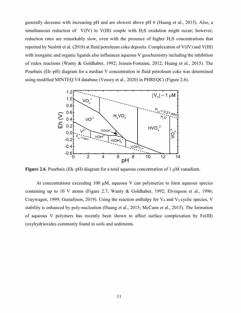
11
generally decrease with increasing pH and are slowest above pH 6 (Huang et al., 2015). Also, a
simultaneous reduction of V(IV) to V(III) couple with H2S oxidation might occur; however,
reduction rates are remarkably slow, even with the presence of higher H2S concentrations that
reported by Nesbitt et al. (2018) at fluid petroleum coke deposits. Complexation of V(IV) and V(III)
with inorganic and organic ligands also influences aqueous V geochemistry including the inhibition
of redox reactions (Wanty & Goldhaber, 1992; Jensen-Fontaine, 2012; Huang et al., 2015). The
Pourbaix (Eh–pH) diagram for a median V concentration in fluid petroleum coke was determined
using modified MINTEQ.V4 database (Vessey et al., 2020) in PHREQCi (Figure 2.6).
Figure 2.6. Pourbaix (Eh–pH) diagram for a total aqueous concentration of 1 μM vanadium.
At concentrations exceeding 100 μM, aqueous V can polymerize to form aqueous species
containing up to 10 V atoms (Figure 2.7; Wanty & Goldhaber, 1992; Elvingson et al., 1996;
Cruywagen, 1999; Gustafsson, 2019). Using the reaction enthalpy for V4 and V5 cyclic species, V
stability is enhanced by poly-nucleation (Huang et al., 2015; McCann et al., 2015). The formation
of aqueous V polymers has recently been shown to affect surface complexation by Fe(III)
(oxyhydr)oxides commonly found in soils and sediments.

12
Figure 2.7. Predominance diagram showing aqueous V(V) speciation as a function of pH and [V]T.
Vanadium species are readily leachable under oxic condition and predominantly as V(V),
although V(IV) has been detected. However, V(IV) is expected to oxidize rapidly to V(V) under
oxic conditions.
Long-term V leaching and mobility within associated coke leachates are complex processes
depending on the interaction of coke with water matrixes, V aqueous speciation, and the
geochemical conditions of coke storage. However, complex interaction mechanisms between coke
and OSPW in the long-term led to a gradual decrease in the aqueous V concentration (Zubot et al.,
2012). This result suggests a dynamic fluctuation in the V partitioning between coke and the aqueous
phase within coke deposits.
2.5.2. Nickel
Strong & Filby (1987) reported a Ni concentration of 62–75 mg kg−1 within Alberta bitumen.
Associated fluid petroleum coke typically exhibits a Ni concentration of 35–719 mg kg−1 (Jack et
al., 1979; Chung, 1996; Kessler & Hendry, 2006; Zubot et al., 2012; Nesbitt et al., 2018, 2017).
Nesbitt et al. (2018) reported that Ni(II) porphyrin complexes are the dominant Ni form in petroleum
coke. Nesbitt et al. (2018) found that X-ray absorption near edge structure (XANES) spectra from
the inner and outer margins of individual concentric layers are usually different, and heterogeneous
distribution and speciation of Ni within coke particles has been discovered, including organic and
inorganic phases. Nickel(II) porphyrin complexes are the dominant form of solid-phase Ni in the
inner region of these concentric layers, while the outer margins contain inorganic Ni(II)-sulfide and
Ni(II)-oxide, constituting a minor component of Ni in fluid coke (Nesbitt et al., 2018). The

13
dominance of porphyrin complexes in fluid petroleum coke is consistent with the geological
petroleum system (Lewan & Maynard, 1982; Lewan, 1984).
Adding Mo(IV)-disulfide (MoS2) along with Ni and Co (supported by alumina, γ–Al2O3, and
silica) as catalysts for the hydro-conversion of bitumen distillates prior to coking may cause Ni to
incorporate into coke particles and therefore could introduce an inorganic source of Ni. In addition,
the catalyst may promote the porphyritic conversion to the sulfide phase (Gray, 2015), providing
another inorganic source of Ni. These inorganic phases, plus the thermal decomposition of porphyrin
complexes during the coking process, results in heterogeneous Ni distribution and speciation within
coke particles (Nesbitt et al., 2018).
Nesbitt et al. (2018) observed enhanced Ni release from fluid petroleum coke at elevated ionic
strength and acidic pH. Also, Nesbitt et al. (2018) reported an aqueous Ni concentration of 2–
120 μg L−1 within coke deposits from the AOSR with a significant negative correlation between
dissolved Ni concentrations and pH. A similar negative correlation between pH and Ni concentration
in coke pore water was discovered by Zajic et al. (1977). Puttaswamy & Liber (2011) reported a Ni
concentration of 145 ± 31 μg L−1 at pH 5.5 in contrast with 0.2 ± 0.1 μg L−1 at pH 9.5 in oil sands
fluid petroleum coke. The observed negative relationship between pH and dissolved Ni
concentrations may result from the pH-dependent variation in net surface charge and sorption of
Ni2+ and positively charged Ni complexation (i.e., NiHCO3+) on the coke surface. This also implies
that the pHPZC (pH point of zero charge) for Ni is an important factor that could control Ni mobility
within fluid coke deposits.
Nickel(II) is the dominant oxidation state of Ni in the environment and it is soluble in most
natural waters, except for at pH > 10 where low-solubility Ni(II) hydroxides are formed and
precipitated (Hummel & Curti, 2003). Nickel is less redox-sensitive than V, existing exclusively in
the Ni(II) oxidation state (Figure 2.8).

14
Figure 2.8. Pourbaix (Eh–pH) diagram for Ni at 0.9 μM total aqueous concentration.
The precipitation of the secondary sulfide phase (i.e., NiS(s), mackinawite [FeS(s)], and pyrite
[FeS2] in the presence of H2S) may limit dissolved Ni concentrations. Incorporation of Ni into the
formed mackinawite and pyrite formed under sulfate-reducing conditions may limit Ni mobility
(Huerta-Diaz et al., 1998; Luther et al., 1980; Rickard, 2012). Aqueous Ni speciation and mobility
is also controlled by the presence of ligands such as sulfate (SO42−), carbonate (CO3
2−), and
bicarbonate (HCO3−; Figure 2.9). Pore water pH, sorption–desorption, complexation, and (co)-
precipitation reactions are the principal controls on dissolved Ni concentration and mobility within
oil sands fluid petroleum coke deposits.
Inorganic Ni is likely the primary long-term source of dissolved Ni in fluid petroleum coke
deposits, and its release and mobility are highly correlated with porewater pH and sorption–
desorption reactions such that: (1) acidic environments lead to high release and mobilisation of Ni,
and (2) alkaline environments can limit the Ni mobility.

15
Figure 2.9. Nickel(II) hydroxide speciation (top), Ni(II) complexation in the presence of sulfate
(1000 mg kg─1; middle), and Ni(II) complexation in open carbonate systems (bottom).
2.5.3. Molybdenum
Fluid petroleum coke typically exhibits Mo concentrations of 7.6–121 mg kg−1 (Jack et al.,
1979; Chung, 1996; Kessler & Hendry, 2006; Zubot et al., 2012; Nesbitt, 2016). Robertson et al.
(2019) reported that Mo occurs as Mo(VI), outer- and inner-sphere complexes, and Mo(IV) in
petroleum coke. A lower proportion of outer-sphere Mo(VI) complexes relative to inner-sphere
complexes was observed by Robertson et al. (2019) in a slurry coke sample, which suggests that
outer-sphere complexes are susceptible to leaching under the geochemical conditions within the
coke deposit.
Although solid-phase Mo concentrations are relatively low compared with V and Ni, Mo
concentrations in pore water within AOSR coke deposits are comparable to dissolved V and Ni
(Nesbitt and Lindsay, 2017; Nesbitt et al., 2018; Robertson et al., 2019). Robertson et al. (2019)
reported a dissolved Mo concentration of 0.097–2.2 mg L─1 within coke deposits, with the maximum

16
concentration below the water table within the mixing zone between slightly acidic and oxic
meteoric water and mildly alkaline and anoxic OSPW. This mixing zone resulted in elevated pH,
electrical conductivity (EC), and ionic strength, and likely mobilized the outer-sphere Mo(VI)
complexes (Robertson et al., 2019). Also, geochemical modeling of pore water within AOSR fluid
petroleum coke deposits suggested that MoO42─ is the dominant aqueous species of Mo(VI);
therefore, the presence of MoO42─ adsorption complexes is possible (Robertson et al., 2019).
Molybdenum exhibits complex aqueous geochemistry and occurs in a range of oxidation
states, and also could form complexes with cations, anions, and organic ligands. Molybdenum(VI)
is the dominant oxidation state in most oxic natural water and is present as tetrahedral MoO42─
(Goldberg et al., 1996; Xu et al., 2013; Smedley & Kinniburgh, 2017). The dissolved Mo
concentration is controlled by aqueous Mo species, pH, redox potential, sorption–desorption, and
precipitation–dissolution reactions (Smedley & Kinniburgh, 2017). The integration of these factors
defines Mo mobility and attenuation within AOSR deposits. Fe-(hydr)oxides, pyrite, clay minerals,
and organic matter are the phases existing within the coke that can adsorb MoO42─; therefore, Mo
mobility and attenuation could be controlled by the presence of these phases and their activity. These
phases have the highest adsorption capacity under mildly acidic conditions since the net surface
charge is positive (~pH 3–6)(Goldberg et al., 1996; Bostick et al., 2003; Gustafsson & Tiberg, 2015).
However, increasing pH and ionic strength would decrease their adsorption capacity, with minimal
adsorption occurring at pH > 8 (Goldberg et al., 1996; Gustafsson & Tiberg, 2015). At circumneutral
to alkaline pH, Mo occurs as soluble molybdate (MoO42─; [Mo(VI)]). Organic matter, clay minerals,
and pyrite exhibit net negative surface charge under these pH conditions, whereas net surface charge
is neutral or slightly negative for Fe-(hydr)oxides phases. Consequently, molybdate adsorption is
typically limited at neutral to alkaline pH (Smedley & Kinniburgh, 2017).
Precipitation of relatively insoluble metal molybdate phases (e.g., NiMoO4, PbMoO4, and
CaMoO4) caused by elevated ionic activities have been reported in neutral to alkaline mine tailings
(Essilfie-Dughan et al., 2011; Conlan et al., 2012; Blanchard et al., 2015) and could limit Mo
concentrations in fluid petroleum coke deposits. Under sulfate-reducing conditions, a series of
intermediate thiomolybdate species including MoO3S2−, MoO2S2
2−, MoOS32−, and MoS4
2− could
form (Figure 2.10; Helz et al., 1996; Xu et al., 2013). These thiomolybdates dominate Mo speciation
in sulfidic environments (Smedley & Kinniburgh, 2017) and are readily attenuated by co-
precipitation or adsorption reactions at mineral surfaces (Helz et al., 1996; Bostick et al., 2003; Das
et al., 2007).

17
Figure 2.10. Pourbaix (Eh–pH) diagram for a median concentration of Mo at 1 μM total aqueous
concentration found within fluid petroleum coke deposits.
Aqueous Mo(VI) polymerizes to form HxMo7O24x−6, where x = 1 to 3, at high [Mo]T (i.e.,
≥10−3 M) and acidic pH (i.e., < 6; Figure 2.11; Xu et al., 2013; Smedley & Kinniburgh, 2017).
Figure 2.11. Predominance diagram showing aqueous Mo(VI) speciation as a function of pH and
[Mo]T.
Since adsorbed MoO42− is readily mobilized in the presence of OSPW, the oxidative
dissolution of MoS2 is likely a principal long-term source of dissolved Mo in fluid petroleum coke
deposits (Robertson et al., 2019). However, MoS2 is both highly insoluble and resistant to oxidative
weathering, suggesting that long-term Mo release may be limited (Lindsay et al., 2015).

18
2.6. Mine Closure Considerations
Oil sands mining operations have disturbed a large land area within the AOSR including
forests and peatlands, primarily fens covering >50% of landscape (Price et al., 2010; Vitt et al.,
1996). Regulations ensure that disturbed land is progressively reclaimed to an acceptable state once
operations have reached the end of their productive life. Therefore, environmental conservation is
considered throughout a project, from planning to reclamation and reforestation. Tailings (fluid fine
tailings [FFT], centrifuged fine tailing [CFT], tailings sand, etc.), petroleum coke, and overburden
within the AOSR will likely be stored together in terrestrial or subaqueous closure landscapes.
However, the interaction between these materials, with different physical and chemical properties,
as well as the potential effects of these interactions on the overall success of a closure system, is a
major concern and needs further investigation.
Petroleum coke can act as a low density, highly permeable aggregate for a light capping on
soft tailings material such as CFT and tailings (Sobkowicz et al., 2012; Simhayov et al., 2017). The
use of petroleum coke as a capillary break between CFT and reclamation material (peat-mineral mix
soil) was investigated by Cilia (2018) and Swerhone (2018). Also, Simhayov et al. (2017) used a
layer of petroleum coke as a construction material to create a self-sustaining, peat accumulating fen-
upland ecosystem. In a fen system, petroleum coke can act as permeable underdrain to distribute the
hydraulic pressure (water and solute flows) beneath the fen. Moreover, several research studies have
investigated the use of petroleum coke for OSPW management including a water treatment option
(Gamal El-Din et al., 2011; Zubot et al., 2012). However, potential leachability of certain trace
elements, reported previously by Nesbitt (2016) and Swerhone (2018), make their applications
limited.
The leachability of elements in petroleum coke depends on the physical and chemical
properties of the coke and the composition of the water that may interact with it. Previous field
studies have examined the potential for metal leaching by meteoric water and OSPW, however it is
possible that petroleum coke may also encounter ARD generated by the oxidative weathering of
froth treatment tailings (Kuznetsov et al., 2015; Lindsay et al., 2019). Metal leachability and the
interaction between petroleum coke and ARD has not been previously established. Therefore, a
better understanding of long-term metal leaching from petroleum coke under different geochemical
conditions relevant to mine closure is critical. The results of this study will improve the
understanding of metal (i.e., V, Ni, and Mo) leaching and mobility within the oil sands mine closure

19
landscape, and will assist decision makers (i.e., mine closure planners) to develop strategies for
integrating coke into closure landscapes while limiting the release and transport of metals.
2.7. Hydrogeophysics
Hydrogeophysics is a research area which uses non-destructive or minimally destructive
methods (i.e., electrical resistivity [ER]; self-potential [SP]) to evaluate hydrogeological parameters
such as permeability and dispersivity, water content, water quality, and biological activity (Naudet
& Revil, 2005; Ntarlagiannis et al., 2005; Rubin & Hubbard, 2005; Williams et al., 2005; Hubbard
& Linde, 2011; Revil et al., 2012; Ahmed et al., 2016).
Electrical resistivity (ER) is an active geophysical method and is performed by injecting a
current waveform through electrodes (sink and source) and measuring the respond voltage difference
through potential electrodes. ER corresponds with water content, temperature, the salinity of pore
water, clay content, and mineralogy (Binley et al., 2015; Singha et al., 2015). Rock texture, pore-
space geometry, and mineralogy are factors that control solute transport processes within the
subsurface and together resulted in spatial-temporal changes in solute concentrations. Knowing the
link between petrophysical properties with geophysical parameters is necessary to interpret and
study the transport process. Coupling geophysical and tracer test have been investigated before as a
tool to resemble solute transport in the subsurface (Binley et al., 2002; Slater et al., 2002; Martínez-
Pagán et al., 2010; Bolève et al., 2011). The inverse problems conditionally can be parametrized to
employ stochastic inversion to determine the probability density of material properties, such as
permeability. Forward and inverse modeling are needed to interpret the measured data at the site or
in the lab (Appendix A).

20
CHAPTER 3: MATERIALS AND METHODS
3.1. Laboratory Columns Experiments
Laboratory column experiments were conducted to assess long-term metal leaching from
fluid petroleum coke during interaction with different water types that could be encountered in oil
sands mine closure landscapes. Based on previous field studies, meteoric water and OSPW are the
two prevalent compositions anticipated in oil sands mine closure landscapes, whereas localized
ARD generation associated with sulfide-mineral oxidation in FTT deposits is possible (Kuznetsov
et al., 2015; Nesbitt et al., 2017; Lindsay et al., 2019), so these water compositions were selected
for experiments (meteoric water was simulated by deionized water [DI]). Two separate
experiments were conducted to (i) examine geochemical controls on long-term metal release and
(ii) determine the timing and extent of long-term metal release.
The first experiment examined long-term metal leaching in a series of small columns. In
these experiments, each solution was continuously passed through a separate column containing
fluid petroleum coke collected directly from a coker unit (dry coke) and another column containing
fluid petroleum coke collected from a hydrotransport line (slurry coke). The second experiment
examined long-term metal leaching in a large column. In this experiment, the three different
solutions were sequentially passed through a column containing dry coke. Hydrogeophysical
methods were used to monitor transport within the large column. Aqueous influent, effluent, and
profile samples were collected from both the small and large columns over time. Solid-phase
samples were collected from all columns at the beginning and end of the experiments.
3.1.1. Small Column Setup
The first laboratory column experiments utilized (i) six acrylic columns measuring 0.225 m
long with 0.078 m inner diameter, (ii) fresh dry and slurry coke, and (iii) acid-washed #20–#40
mesh Ottawa sand (Figure 3.1). All small columns were packed with 16.5 cm fresh dry coke (n =
3) or fresh slurry coke (n = 3) placed between two layers of 0.03 m acid-washed sand (AWS). The
AWS layers were placed at the top lower and upper layer and used to direct a homogeneous flow
of water through the coke layer (middle layer). Nylon mesh screen (No. 125) was used to separate
the coke from the acid-washed sand layers. The layers were packed to ensure that the bulk density

21
was consistent along the column and among all columns for each material (Appendix B). Sampling
tubes were installed within sampling ports at 0.03 m intervals from 0.035 m to 0.185 m relative to
the column base. Sampling tubes, constructed from polyfluorotetraethylene (PTFE) tubes, were
installed into each sampling port to facilitate pore water sampling. These 0.08 m samplers were
sealed at one end and perforated along their length prior to installation. Following installation, the
tubes were sealed into the ports with cyanoacrylate crazy glue, and two-way stopcocks were
attached to facilitate sampling via syringe (Figure 3.1).
Each column was fitted with one inlet and one outlet port. The inlet port was connected to a
high-precision, low-flow multi-channel peristaltic pump (Model 2058, Watson-Marlow, Inc.)
using PTFE tubing. The outlet port was connected in series to a sealed overflow sampling cell and
then an overflow waste container. Before starting the experiment, the columns were flushed for 48
h with CO2(g), which is highly soluble in water, and therefore minimizes bubble entrapment during
initial water saturation.
Figure 3.1. Schematic diagram and photo of the small column experiments. The coke layers were
placed between two acid washed sand (AWS) layers.
3.1.2. Large Column Setup
The second laboratory column experiment (sequential water input with different
compositions) utilized (i) one PVC column measuring 0.67 m long with 0.162 m inner diameter,
(ii) fresh dry coke, and (iii) acid-washed #20–40 mesh Ottawa sand (Figure 3.2). The column was
packed with 0.5 m of fresh dry coke between two 0.085 m layers of acid-washed sand. In order to

22
avoid mixing of acid-washed sand with coke, a nylon mesh screen (No. 125) was placed between
these two layers. Packing ensured that the bulk density was consistent along the column (Appendix
B). Five sampling ports were positioned at 0.10, 0.15, 0.25, 0.35, and 0.40 m from the base of the
coke layer and equipped with pore water suction samplers (Rhizon MOM, Rhizosphere Research
Products B.V., The Netherlands). These sampling ports were sealed with a cyanoacrylate crazy
glue to prevent leaks. Non-polarizing Ag/AgCl pellet electrodes (n = 11) were installed at intervals
of 0.05 m along the column for time-lapse SP geophysical method measurements, from 0.115 m
to 0.615 m from the column base. These electrodes were used to measure the voltage differences
between each electrode and the reference electrode (the last electrode). A platinum wire was cut
into 0.01 m long pieces to use as an electrode for time-lapse geophysical resistivity measurements.
Four electrodes were positioned at 90° angles in a ring configuration at 0.09 m intervals, except
for the first and last that were at 0.05 m intervals, from 0.06 m to 0.61 m from the column base.
This configuration was based on sensitivity analysis performed using COMSOL Multiphysics
(COMSOL Multiphysics® v.5.4). The large column was instrumented with eight platinum rings
and 11 Ag/AgCl pellet electrodes. Time-lapse geophysical measurements (ER, SP) were
performed using the IRIS (Syscal, France) instrument during the tracer tests (twice a day, every
12 h), and recorded data were prepared for geophysical modeling.
Figure 3.2. Graphical representation of the placement of platinum wire (left); schematic
representation of column experiment (middle); photograph of the fully constructed column (right).
23
The large column was fitted with one inlet and one outlet port. The inlet port was connected
to a high-precision, low-flow multi-channel peristaltic pump (Model 2058, Watson-Marlow, Inc.)
using PTFE tubing. Overflow sampling cell was sealed, and then in series outlet port, overflow
sampling cell and waste jug were all connected using PTFE tubing. Before starting the experiment,
the columns were flushed for 48 h with CO2(g), which is highly soluble in water, and therefore
minimizes bubble entrapment during initial water saturation.
3.1.3. Input Solutions
Input solutions were prepared in 5 L acid-washed amber glass media bottles using DI water
and ACS reagent-grade salts. The composition of synthetic OSPW and ARD solutions were based
on previous studies (Dompierre et al., 2017; Lindsay et al., 2019; Table 3.1). The synthetic OSPW
solution was prepared by dissolving (g L−1) NaCl (1.78), NaHCO3 (1.34), MgSO4•7H2O (0.203),
CaSO4•2H2O (0.172), KCl (0.038), and Na2SO4 (0.037) into DI water. While continuously stirring,
the solution was purged with CO2(g) overnight and then with compressed air for 24 h until the
solution pH stabilized at approximately 8.4. The synthetic ARD solution was prepared by
dissolving (g L−1) Fe2(SO4)3•xH2O (11.2), MgSO4•7H2O (2.03), CaSO4•2H2O (1.72), Na2SO4
(0.315) and NaCl (0.248) in DI water. The ARD solution was adjusted to pH 2.0 using concentrated
H2SO4. The simulated meteoric water solution was prepared by bubbling DI with air overnight to
ensure equilibration with atmospheric gases. The sequential leaching experiment (large column
experiment) also included OSPW collected from an oil sands mine as an input solution (field
OSPW). All input solutions were vacuum filtered through 0.45 μm cellulose filter paper (Whatman
acetate membranes, GE Healthcare, USA) to remove any precipitated solids, and transferred to
clean acid-washed amber glass media bottles. The solutions were pumped in an upward direction
to avoid gravity drainage through the columns. The peristaltic pumps were calibrated to achieve
approximated flow rates of 49 and 460 mL d−1 for the small columns and large column,
respectively. Column discharge was monitored over time and tracer tests were performed to
determine pore water velocity, column hydrodynamic properties (i.e., dispersivity and porosity),
and residence time. A mylar balloon containing 100% (v/v) N2(g) was attached to the input solution
reservoir during the field OSPW input phase of the large column experiment to limit O2(aq)
concentrations.

24
Table 3.1. Target input solution composition.
Parameter Units DIa OSPWb OSPWc ARDd
pH 7.2 8.6 8.86 2.0
Na mg L−1 2.97 1060 1160 200
Mg mg L−1 0.02 20 6.54 200
K mg L−1 0.2 20 12.5 0.4
Ca mg L−1 0.25 12.5 5.96 400
HCO3 mg L−1 13.4 870 1120 0
Cl mg L−1 0.41 1100 900* 150
SO4 mg L−1 0.25 200 592 10000
Fe mg L−1 0 0 0 2460
*Cl concentration was assessed using charge balance error (CBE) calculated by PHREEQCi
aDI: Deionized water
bOSPW: synthetic oil sand process-affected water
cOSPW: Oil sand process-affected water
dARD: Acid rock drainage
3.2. Aqueous-Phase Analyses
Column influent and effluent samples were collected weekly from the input solution
reservoir and the effluent sampling cells. Daily effluent sampling was also performed during the
first pore volume to capture initial element leaching. Profile sampling of the column pore water
was performed every two months for the small columns and monthly for the large column. These
frequencies were chosen for profile sampling to limit disturbances to the column flow regime. All
water samples were collected into clean all-plastic polypropylene (PP) syringes (Norm-Ject®,
Henke-Sass Wolf GmbH, Germany).
Pore water pH, reduction–oxidation potential (Eh), EC, temperature, and alkalinity were
measured immediately following sample collection. Before each measurement, calibration of the
pH probe (Orion 8156BNUWP ROSS Ultra, Thermo Fisher Scientific, USA) was done using a 3-
point calibration with NIST traceable pH 4, 7, and 10 buffer solutions. The Eh electrode (Orion
9678BNWP Sureflow, Thermo Fisher Scientific, USA) performance was checked by Light’s

25
(Light, 1972) and ZoBell’s (Nordstrom, 1977; ZoBell, 1946) solutions (Ricca Chemical Co.,
USA). A standard solution of NaCl with 1413 μS cm−1 (Thermo Scientific, USA) was used to
calibrate the EC electrode. The pH and Eh measurements were performed on unfiltered samples,
and EC and alkalinity measurements were performed on samples filtered through 0.45 μm
polyethersulfone (PES) syringe filter membranes (Minisart, Sartorius AG, Germany). Electrode
performance (pH, Eh, EC) was checked between each measurement, and re-calibration was
completed as required. Alkalinity was determined by titration with 0.16 N or 1.6 N H2SO4 (Hach
Co., USA) to the bromocresol green/methyl red endpoint (Ricca Chemical Co., USA).
Samples for quantification of inorganic anions, major cations, and trace elements were
passed through 0.45 μm, 0.2 μm, and 0.1 μm PES filter membranes (Minisart, Sartorius AG,
Germany), respectively, and stored in high-density polyethylene (HDPE) bottles (Nalge Nunc
International Corp., USA). Samples for cations and trace element analyses were acidified to pH <
2 using concentrated trace metal grade HNO3 (OmniTrace, EMD Millipore, USA). All samples
(inorganic anions, cations, trace elements) were kept at 4 °C until analysis. Analysis of major
cations and trace elements was performed by inductively coupled plasma–optical emission
spectrometry (ICP-OES; SPECTROBLUE, Spectro analytical instruments, Germany), and
inductively coupled plasma–mass spectrometry (ICP-MS; NexION 300D). Major anion
concentrations were measured by ion chromatography (IC; ICS2100; Dionex Corporation).
3.3. Solid-Phase Analyses
Samples of fluid petroleum coke solids were collected during column setup for physical,
chemical, and mineralogical analyses. Two samples from each small column (n =12) were
collected at 0.1 m intervals from the large column (n = 5). These samples were sealed in 50 mL
PE centrifuge tubes and stored at −20 °C until analysis.
3.3.1. Specific Surface Area Analyses
The SSA was determined using Brunauer-Emmett-Teller N2 adsorption isotherms, utilizing
a BET ASAP 2020 surface area analyzer (Micromeritics, Georgia, USA; Brunauer et al., 1938).
Also, the Barrett-Joyncer-Halenda (BJH) method was used to calculate adsorption and desorption
of surface area, pore volume, and pore size. Samples were heated 60 °C for 24 h to remove any
moisture and absorbed gases on the coke particle surface prior to analyses.

26
3.3.2. Particle Size Distribution
Particle size distributions (PSD) for dry coke, slurry coke, and acid-washed sand were
determined by passing the samples through standard test sieves arranged in descending order of
mesh size, based on ASTM D422–63. For each sample (i.e., acid-washed sand, dry and slurry
coke), 400 g of sample was weighed before putting the sample on a shaker. Samples were shaken
for 20 min, and the mass retained in each sieve was weighed to determine the PSD using percent
passing by mass.
3.3.3. Electron Microscopy
Scanning electron microscopy (SEM; Hitachi FE-SEM SU8010, Japan) was performed on
the bulk freeze-dried samples mounted on carbon tape without coating, using a 3 kV acceleration
voltage to capture the micro-scale morphology of coke particles. Electron microprobe analysis
(EMPA; JEOL JXA-8600 Superprobe Microanalyzer, Japan) was used to investigate the internal
chemical composition of discrete particles hosted within coke prepared as thin sections. Thin
sections were coated with a 200 Å carbon layer using the JEOL JEE-4X carbon vacuum evaporator
prior to EMPA analysis.
3.3.4. Cation Exchange Capacity Analysis
The cation exchange capacity (CEC) and exchangeable cation composition are important
factors in water-sediment interactions. Methylene blue has a high binding affinity compared with
inorganic cations (e.g. AgTU, LiCl), as the polar and non-polar components make methylene blue
able to bind well with the surface. Also, the methylene blue test is the method least impacted by
the presence of carbonate mineral phases (Holden et al., 2012). CEC was evaluated for oven-dried
fresh dry (n = 4) and slurry coke (n = 4) using combined methods described by Holden et al. (2012),
Kaminsky (2014), and Santamarina et al. (2002; Appendix C).
3.3.5. pH Point of Zero Charge
The pH point of zero charge (pHPZC) for dry and slurry coke particles was determined using
combined solid addition methods described by Pourrezaei et al. (2014), Alam et al. (2016), and
Robertson et al. (2019). Prior to the experiment, 1 L 0.1 N NaCl, as a background electrolyte
solution, was purged with N2(g) for 24 h in an anaerobic chamber (Coy Laboratory Products, USA;
≤5 vol% H2(g), balance N2(g)) to remove the buffering effect of dissolved CO2 in solution (Alam et
al., 2016). For each sample, nine 40 mL amber vials were labeled with the sample name and desired

27
pH (2, 3, 4, 5, 6, 7, 8, 9, 10). Each amber bottle was filled with 25 mL purged 0.1 M NaCl solution,
and the pH was adjusted with a small volume of 0.1 or 1 M HCl or NaOH. The pH for each amber
vial was measured again and recorded after 1 h to ensure they had reached equilibrium. Adding
0.1 N HCl or NaOH was continued until the actual pH was within ± 0.3 of the target pH. Then, 0.5
g gently-ground, homogenized, and air-dried coke was added to each amber vial, and the amber
bottles were sealed immediately with gas-impermeable rubber-lined septa. All steps were
performed in an anoxic chamber, except weighing. Amber vials were removed from the anaerobic
chamber and placed on an orbital shaker at 100 rpm for 48 h, after which the pH of suspension
was measured again. The change in pH (ΔpH) versus initial pH (pH0) was plotted, and the point
of intersection of the curve with the x-axis (pH0) is associated with pHPZC (Pourrezaei et al., 2014;
Alam et al., 2016).
3.3.6. Elemental Analyses
Total C and S were determined by combustion and infrared detection of evolved CO2 and
SO2 (CS230 Carbon/Sulfur Determinator, LECO Corporation, USA). Concentrations of major and
trace elements were quantified by Li borate fusion digestion followed by ICP-OES and ICP-MS,
respectively. A modified aqua regia (1:1:1 HNO3:HCl:DI) digestion for 1 h at 80 °C followed by
ICP-MS was used to determine As and Se concentrations.
3.4. Data Analysis
3.4.1. Statistical Methods
The Pearson correlation was performed on bulk elemental results; correlation matrixes were
generated using the following procedure to examine the significance and robustness of
correlations. Prior to analysis, a center log-ratio transformation was carried out; the individual
element concentration was divided by the geometric mean of all elements for the same sample.
Then, the log10 of the result was calculated. Such a transformation of values is used to make an
open data set with the sum of elemental concentrations equal to zero. All statistical analyses were
executed on all submitted samples (n = 17) and results were reported for the same sample size (n
= 35) and significance level of 5% (i.e., ρ = 0.05).
28
3.4.2. Transport Parameters
A tracer test using a conservative tracer with initial concentration of zero throughout the
system (Co = 0) was carried out on the columns to determine the pore water velocity, dispersivity
coefficient, porosity, and residence time. A tracer solution containing 100 mg L−1 Br− (from NaBr)
was prepared, and the bromide electrode (Orion 9635BNWP, Thermo Scientific, USA)
performance and sensitivity was checked prior to measurements. A series of different
concentrations of the Br− solution was prepared (0, 2.5, 3, 5, 10, 20, 25, 30, 50, 80, 90, 100 and
200 mg L−1), and a 10-fold difference in concentration should result in a difference of 57 ± 3 mV.
Based on this test, the probe sensitivity was determined to be 2.5 mg L−1, which means ±2.5% is
the electrode sensitivity. A breakthrough curve is the ratio of C/Co versus the number of passed
pore volumes of effluent collected (or time). The column hydraulic parameters (i.e., dispersivity)
and average linear pore-water velocity were determined by solving the equation 3.1 obtained from
Genuchten (1982) which was written and solved for the Br breakthrough curve in MATLAB.
𝜕𝐶
𝜕𝑡 = 𝐷
𝜕2 𝐶
𝜕𝑥2 − 𝑉𝑤 𝜕𝐶
𝜕𝑥 (3.1)
where D is the hydrodynamic dispersion coefficient (L2 T−1), which could be measured with
equation 3.2, and Vw is the average linear pore water velocity (L T−1).
𝐷 = 𝛼𝑉𝑤 + 𝐷∗ (3.2)
In equation 3.2, D* is the effective diffusion coefficient of molecule (L2 T−1) and calculated
with 𝐷∗ = 𝜔 ∗ 𝐷𝑑 ,where 𝜔 is coefficient that is related to the tortuosity and here is considered
0.7 based on Perkins and Johnston, 1963 study for uniform sand column. The first term of equation
3.2 is the mechanical dispersion, where α is the dispersivity coefficient (L).
The column discharge rates were monitored throughout the leaching experiment and tracer
test by weighing the waste container over time, as this is an important factor in measuring
cumulative mass release. The residence time for the columns was determined by finding the time
associated with C/Co = 0.5, which means the Br− concentration in the column effluent is equal to
half of the influent Br− concentration. Pore volume (PV) calculated by multiplying the residence
time (T) by the discharge volume (L3 T−1) over associated time of the residence time. Finally, the
effective porosity was calculated using equation 3.3, dividing PV over the total volume of column.
𝑛𝑒 = 𝑃𝑉
𝑉𝑇 (3.3)

29
3.4.3. Geochemical Modelling
Thermodynamic equilibrium modeling using PHREEQCi (version 3.6.1–15000; Parkhurst
& Appelo, 2013) with a modified Minteq version 3.1 database (Gustafsson, 2018) was performed
to assess data quality, saturation indices, and trace element speciation occurring in the pore water.
Saturation indices were determined from the modeling output to indicate which mineral
phases are most likely present in or out of solution. The charge balance error (CBE) calculated by
equation 3.4 inside the PHREEQC model is an indication of data quality, where a CBE of less than
5% is generally acceptable.
𝐶𝐵𝐸 (%) = (∑ 𝑐𝑎𝑡𝑖𝑜𝑛𝑠+∑ 𝑎𝑛𝑖𝑜𝑛𝑠)
(∑ 𝑐𝑎𝑡𝑖𝑜𝑛𝑠−∑ 𝑎𝑛𝑖𝑜𝑛𝑠)∗ 100 (3.4)
Access to a corrected thermodynamic database for various reactions that can occur is
important in order to understand the water chemistry of V. The redox reactions and associated
equilibrium constants were obtained from Allison et al. (1991) and Wanty and Goldhaber (1992),
as these two databases were in good agreement.
Under strong anoxic conditions, like sulfide-containing sediments or wetlands, V(III) is
expected to be stable. Assuming similar water chemistry between V(III) and Fe3+ (Gustafsson,
2019), thermodynamic data for V(III) hydrolysis were chosen from Buglyó et al. (2005).
Depending on the pH, V(V) will occur in a different coordination environment. At low pH
(pH < 3.6), V(V) presents as VO2+, while at high pH, it presents as the HnVO4
(3-n)− ion (i.e.,
HVO42−). Also, V has a tendency to form poly-nuclear species at concentrations exceeding 100
μM that may consist of up to 10 V atoms (V2, V3, V4, V5, V6, and V10). Mononuclear and poly-
nuclear V reactions and equilibrium constants were considered from Larson (1995), Cruywagen
et al. (1996), Elvingson et al. (1996), Cruywagen (1999), Smith et al. (2004), and McCann et al.
(2015, 2013; Appendix D).
3.4.4. Geophysical Modeling
This section describes the low-frequency geoelectrical methods (i.e., SP and ER) and their
application in solving practical hydrogeological problems. These techniques can be used to
monitor the interaction of pore water minerals and to evaluate hydrodynamic parameters. These
methods should be used in parallel with additional data from other in situ tests (e.g., chemical
analysis of porewater) to help verify the geoelectrical results. Electrical geophysical computer
modeling falls into two categories: (i) forward and (ii) inverse modeling. Forward modeling is the

30
simulation of a response, given a set number of parameters, to identify a solution. Forward
modeling is usually solved numerically using finite-difference or finite-element methods (i.e.,
COMSOL Multiphysics). Inverse modeling evaluates the optimal parameters given a specific
acquired dataset.
The geometric factor (Kg) for the ring and lateral (A, B, C, and D; Wenner array
configuration) positions were calculated in COMSOL Multiphysics assuming a constant resistivity
throughout the column and current of 1 A. The inversion model, given the measured voltage and
current (∆𝑉
𝐼) over time with calculated geometric factors, was carried out by multiplying the
geometric factor by the ratio of voltage over current to calculate the apparent resistivity (ohm m).
The calculated apparent resistivity was plotted over time for each individual ring. Based on
midpoints theory, the time for the apparent resistivity to reach the median value was determined
for each individual ring during the first tracer test (including the injection and decay). The average
linear velocity was measured using a linear regression of locations vs. mid-point time for the
individual ring.
Forward 1-D time dependent modeling was performed in COMSOL Multiphysics using the
direct currents (AC/DC) module. Chemical species, including Na+, Br−, SO42−, Al3+, Fe2+, Ca2+,
Mg2+, and alkalinity were considered in the transport model—transport equation 3.5 was solved
for each individual species. Their associated diffusion coefficients were obtained from Yuan-Hui
and Gregory (1974). Also, as coke is a reactive material, the reaction rates for individual species
(Ri) were determined by finding the best fit to measured concentrations in the column effluent
(Appendix A).
𝜕𝐶
𝜕𝑡+ 𝛻. 𝐽𝑖 + 𝑢. 𝛻𝐶𝑖 = 𝑅𝑖 (3.5)
where Ji is hydrodynamic dispersion and is equal to −Di * ∇Ci , u is the pore water velocity.
The transport equation (equation 3.5) was solved as a function of time for these chemical species,
and their aqueous concentrations were converted to EC using the Kohlrausch’s law of independent
ionic mobility (equation 3.6); where the EC of a solution is equal to the sum of EC of all aqueous
species in the solution. The Kohlrausch’s law covers complete and partial ionisation that typically
represented by strong and weak electrolytes, respectively. Thus, the salt-type solute for this
experiment was assumed as a strong electrolyte and the molar conductivities as a function of
electrolyte concentration for each individual species is linear. In order to measure the EC of

31
individual species, the concentration of the individual species (M m−3), νi, was multiplied by the
molar ionic conductivity (mS m2 M−1), λi, obtained from Adamson (1973).
𝛬 𝑚° = ∑ 𝜐𝑖𝑖 ∗ 𝜆𝑖 (3.6)
Finally, Archie’s law (Archie, 1942) is used to calculate the apparent resistivity of individual
ring with porosity and EC of the pore fluid (Equation 3.7). The fitting parameter m, could be
estimated based on initial values of R, Rw and porosity (φ).
𝜎0 = 𝜎𝑤 𝜑𝑚 (3.7)
3.4.5. Cumulative Mass Release Calculations
Cumulative mass release calculations were performed to determine the metal leaching for
coke under different geochemical conditions (including DI, OSPW, and ARD) using equation 3.8.
∆𝑀𝑗 = ∑ 𝑀𝑗𝑂𝑢𝑡𝑓𝑙𝑜𝑤 − ∑ 𝑀𝑗𝐼𝑛𝑓𝑙𝑜𝑤 (3.8)
where 𝑀𝑗𝑂𝑢𝑡𝑓𝑙𝑜𝑤 and 𝑀𝑗𝐼𝑓𝑙𝑜𝑤 are masses for a given solute, j, were calculated with equation
3.9 as the product of water volume (L), 𝑑𝑉𝑖, over a given sampling interval, 𝑖, and the mean
concentration (µg L−1) of the solute, 𝑚𝑗,𝑖, over that time interval.
𝑀𝑗,𝑖 = 𝑑𝑉𝑖 𝑚𝑗,𝑖 (3.9)
The cumulative mass, ∑ 𝑀𝑗, in and out were determined with equation 3.10 by summing 𝑀𝑗,𝑖
over time:
∑ 𝑀𝑗 = ∑ 𝑀𝑗,𝑖𝑛𝑖=1 (3.10)

32
CHAPTER 4: RESULTS AND DISCUSSION
4.1. Physical Characteristics
Coke solids exhibit a spherical to sub-spherical shape and typically range from 40 to 500 μm
in diameter (Figure 4.1). Given its uniform spherical shape with a sandy texture and the measured
PSD for slurry and dry coke samples, coke can be classified as a moderately well-sorted sand with
low fines (uniformity coefficient [CU] ⁓2; Table 4.1).
Coke particles display fractures and broken pieces that may result from heating and cooling
cycles in the coking process or during slurry preparation when hot coke particles are mixed with
OSPW prior to hydrotransport (Figure 4.1). These features (i.e., fracturing and broken pieces) are
attributed to the thermal shock on coke particles. Also, some attached particles observed on the
surface of slurry coke particles might have settled on the coke surface during slurry preparation or
hydrotransport. More cracks and broken pieces were observed on slurry coke samples compared
with dry coke samples (Figure 4.1), suggesting that slurry coke preparation promotes fracturing,
broken particles, and particle attachment on the coke surface.
Table 4.1. Physical properties of acid-washed sand (AWS) and coke.
Source d10 d60 Cua SSAb pHPZCc CECd
(mm) (mm) (m2 g−1) (meq 100 g −1)
DCe 0.1 0.27 2.7 0.25 ± 0.18 6.65 ± 0.17 0.032 ± 0.013
SCf 0.12 0.27 2.25 6.5 ± 0.48 7.19 ± 0.17 0.203 ± 0.007
AWSg 0.3 0.60 2 – – – aCu: Uniformity coefficient (d60/d10)
bSSA: Specific surface area
cpHPZC: pH point of zero charge
dCEC: Cation exchange capacity
eDC: Dry coke
fSC: Slurry coke
gAWS: Acid washed sand
Although the SSA for coke samples is generally low, more fractured and broken pieces and
attached particles on the slurry coke surface compared with the dry coke samples resulted in higher

33
SSA for slurry coke (Table 4.1). The measured SSA for coke is generally consistent with
previously reported values of 4.5 ± 2.8 m2 g
─1 (Nesbitt et al., 2017), 6 m2 g−1 (Zubot et al., 2012),
8 m2 g−1 (Pourrezaei et al., 2014), 10 m2 g−1 (Har, 1981), and 11 m2 g−1 (Fedorak & Coy, 2006)
for similar samples collected from coke deposits or coker units.
Figure 4.1. Scanning electron microprobe (SEM) images of fluid petroleum coke; (a) dry coke,
(b) slurry coke, (c, d) dry coke, and (e, f) slurry coke.
The average pHPCZ values for fresh dry and slurry coke were 6.65 ± 0.17 and 7.19 ± 0.17,
respectively (Table 4.1, Appendix E). These values were consistent with previous studies of oil
sands fluid petroleum coke by Pourrezaei et al. (2014), Nesbitt et al. (2018), and Robertson et al.
(2019), yet substantially higher than the pHPCZ of 2.5 reported by Alam et al. (2016). Coke particles
exhibit net positive and net negative surface charges when in contact with solution having a pH
34
below and above the pHPCZ of 6.7–7.2, respectively. This has implications for the mobility of
aqueous metal ions in coke deposits and in mine closure landscapes.
4.2. Chemical Characteristics
The chemical composition of fluid petroleum coke samples is dominated by C (79.25 ± 1.34
wt%) and S (8.00 ± 0.13 wt%), which are associated with bitumen (Figure 4.2, Appendix F).
Elevated concentrations of several major elements including Si (12760 ± 945 mg kg−1), Al (7000
± 180 mg kg−1), Fe (5200 ± 200 mg kg−1), Ti (1400 ± 70 mg kg−1), Ca (2000 ± 180 mg kg−1), K
(1060 ± 45 mg kg−1), and Mg (790 ± 40 mg kg−1) are largely attributed to entrained solids (Nesbitt
et al., 2017). Potentially hazardous trace metals including V (1380 ± 45 mg kg−1), Ni (540 ± 18
mg kg−1), and Mo (75.1 ± 3.5 mg kg−1) were also detected. Har (1981) reported volatile elements
including H (1.5–1.67 wt%), N (1.3–1.6 wt%), and O (2.3–2.5 wt%) which are lost on ignition.
Very similar volatile element concentrations also have been reported previously by Chung (1996)
and Kessler & Hendry (2006).
Solid-phase concentrations of major and trace elements are generally consistent with
previous studies of fluid petroleum coke (Table 4.2). Exceptions include Ni concentrations
previously reported by Zubot et al. (2012) and Mo concentrations previously reported by Nesbitt
et al. (2017) and Zubot et al. (2012). Nickel concentrations were 513–573 mg kg−1 for samples
analyzed in this study, while Zubot et al. (2012) reported 35–68 mg kg−1. Similarly, Mo
concentrations were 71–85 mg kg−1 in this study compared to 7.6–29 mg kg−1 reported by Zubot
et al. (2012) and Nesbitt et al. (2017). Some previous studies analyzed samples collected
immediately from coker units or hydrotransport lines (Jack et al., 1979; Har, 1981; Zubot et al.,
2012), whereas other studies analyzed samples from coke deposits subjected to extended periods
of weathering (Chung, 1996; Kessler & Hendry, 2006; Nesbitt et al., 2017). Variability in reported
values could result from differences in bitumen feedstock, sampling location, weathering extent,
or analytical methods.

35
Figure 4.2. Bulk elemental analyses for elements in fluid petroleum coke. Box lines define 25th,
50th, and 75th percentiles; lower and upper whiskers define 10th and 90th percentiles.
Coke particles consisted of a series of sub-spherical, successive concentric layers. Each
concentric layer was composed of two zones: (i) an inner region measuring 5–10 μm thick; and
(ii) an outer margin measuring 1–5 μm thick. In addition, the outer region was a lighter color
compared with the inner region in backscattered electron (BSE) images (Figure 4.3), which
suggests more elements with a higher atomic number are present.

36
Table 4.2. Summary of selected elemental contents for fluid petroleum coke samples collected
from coker units and field deposits.
Source n C S V Ni Mo
(wt.%) (wt.%) (mg kg−1) (mg kg−1) (mg kg−1)
cokera 1 82 3.3 1600 660 121
cokerb 10 79–82 5.8–7.1 1500–1900 550–720 –
depositc 5 80–84 6.1–-6.9 1600–1766 475–520 66–100
depositd 3 78–84 7.0–8.1 1134–1440 470–590 67–94
cokere 29 75–89 5.6–7.6 1000–1400 35–68 12–29
depositf 28 80–89 6.4–7.6 1000–1500 130–460 7.6–23
cokerg 11 78–82 7.8–8.4 1300–1400 510–570 71–78
depositg 6 74–82 7.9–8.1 1400–1500 520–570 72–85 aJack et al. (1979) bHar (1981) cChung (1996) dKessler & Hendry (2006) eZubot et al. (2012) fNesbitt et al. (2017) gThis study
Energy dispersive X-ray (EDX) spectra of the inner and outer margins of individual layers
revealed that the chemistry of the inner region of individual layers is dominated by S, Al, and Si,
while the outer margin of these layers have elevated K, Ca, Ti, V, Mn, and Fe concentrations
(Figure 4.3). Successive concentric layers with different chemistry were reported by Nesbitt et al.
(2017). The coking cycle process, including material adding and thermal decomposition of organic
components, resulted in successive concentric layers with different chemistry (Zubot et al., 2012;
Nesbitt et al., 2017).
Bulk C and S concentrations exhibited a strong positive correlation (r = 0.97). This positive
correlation was attributed to the fact that the chemical composition of coke is dominated by C and
S. Statistical analysis revealed a strong positive correlation between V and Ni with both C (r =
0.92) and S (r = 0.95). The correlation of V and Ni with C is attributed to the prevalence of V(IV)
and Ni(II) porphyrins in fluid coke samples (Nesbitt & Lindsay, 2017; Nesbitt et al., 2018, 2017).
Also, the correlation between C, S, and metals is consistent with Nesbitt et al. (2017). There was
also a strong positive correlation between Mo, C (r = 0.88), and S (r = 0.90) within coke bulk
concentrations.

37
Figure 4.3. Top: Backscattered electron (BSE) images of fluid coke particles in thin section.
Yellow dots and labels denote the energy dispersive X-ray (EDX) spectra for sample A (top) and
sample D (bottom). Yellow dots indicate locations of the obtained spectra while the points without
a red dot spectra was obtained for that specific mineral.
Iron and Ti exhibited a strong positive correlation (r = 0.88), which indicates their
association with oxide phases. Obtained EDX spectra at the outer margin of individual layers
exhibited relatively higher Ti and Fe content than the inner regions. In addition, discrete grains of
pyrite (FeS2; D1) and titanium oxide like rutile or anatase (i.e., TiO2; D2, D4) were observed within
coke particles (Figure 4.3). The presence of a Ti-bearing phase throughout the coke matrix was
previously reported by Nesbitt et al. (2017). Regions with elevated concentration of co-located
sub-micron Fe- and Ti-bearing phases within coke grains was reported by Nesbitt et al. (2017).
38
The presence of Fe- and Ti-bearing phases hosted in coke may act as adsorption sites for aqueous
trace metals (Blackmore et al., 1996; Zubot et al., 2012).
Correlation between Si, Al, K, and Mg (r = 0.72–0.91) was attributed to their co-occurrence
in entrained aluminosilicate phases within fluid petroleum coke particles. Si, Al, K, Ca, and Mg
were detected through the obtained EDX spectra of coke particles (Figure 4.3). This is in
agreement with Nesbitt et al. (2017) who showed that distinct Si-bearing particles and sub-micron
sized particles containing Al, K, Mg, and Si have been reported. A high correlation between Ca
and Sr (r = 0.75) was observed within bulk coke, and suggests the presence of carbonate minerals.
The presence of carbonate minerals in fluid coke particles was also reported by Kessler & Hendry
(2006) and Nesbitt et al. (2017). Elevated Al, Si, K, Ca, Ti, V, and Fe at the outer margin of
individual layers compared with the inner margin could be attributed to material addition and coke
surface coking during each cycle within the coker units.
4.3. Small Columns
4.3.1. Aqueous Geochemistry
The pH of the influent was relatively stable during the experiments, with a median value of
7.21, 8.60, and 2.04 for DI, OSPW, and ARD, respectively. Compared with the influent, the
effluent pH declined for the DI solution, to 4.48–5.40 for dry coke and 4.70–6.40 for slurry coke.
The pH of the OSPW effluent solution was 6.10–6.80 for dry coke and 6.10–6.90 for slurry coke.
The pH of the ARD effluent solution was 1.90–2.60 and 1.90–3.30 for dry and slurry coke,
respectively. The pH of the influent and effluent under ARD is generally similar except for the
first two pore volumes for the column with slurry coke, which had a higher pH due to acid
neutralization by the residual OSPW on the coke surface (Figure 4.4).
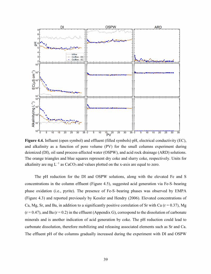
39
Figure 4.4. Influent (open symbol) and effluent (filled symbols) pH, electrical conductivity (EC),
and alkalinity as a function of pore volume (PV) for the small columns experiment during
deionized (DI), oil sand process-affected water (OSPW), and acid rock drainage (ARD) solutions.
The orange triangles and blue squares represent dry coke and slurry coke, respectively. Units for
alkalinity are mg L−1 as CaCO3 and values plotted on the x-axis are equal to zero.
The pH reduction for the DI and OSPW solutions, along with the elevated Fe and S
concentrations in the column effluent (Figure 4.5), suggested acid generation via Fe-S–bearing
phase oxidation (i.e., pyrite). The presence of Fe-S–bearing phases was observed by EMPA
(Figure 4.3) and reported previously by Kessler and Hendry (2006). Elevated concentrations of
Ca, Mg, Sr, and Ba, in addition to a significantly positive correlation of Sr with Ca (r = 0.37), Mg
(r = 0.47), and Ba (r = 0.2) in the effluent (Appendix G), correspond to the dissolution of carbonate
minerals and is another indication of acid generation by coke. The pH reduction could lead to
carbonate dissolution, therefore mobilizing and releasing associated elements such as Sr and Ca.
The effluent pH of the columns gradually increased during the experiment with DI and OSPW

40
inputs for both dry and slurry coke, suggesting a decrease in the acid generation potential for coke
(Figure 4.4).
Figure 4.5. Influent (open symbol) and effluent (filled symbols) dissolved concentration of S and
Fe as a function of pore volume (PV) for the small columns experiment during deionized (DI) and
oil sand process-affected water (OSPW) solutions. The orange triangles and blue squares represent
dry and slurry coke, respectively. Values plotted on the x-axis are equal to zero.
Thermodynamic modeling indicated that the initial pH of the effluent was strongly
influenced by CO2(g) dissolution, associated with column setup, and washing of the residual OSPW
from the slurry coke sample. The dissolved CO2(g) promoted carbonate dissolution and ion-
exchange reactions over the first one to two pore volumes.
The influent EC and alkalinity of all solutions were relatively consistent over the experiment.
The median EC for the influent solutions was 10.8 µS cm−1 for DI, 4.84 mS cm−1 for OSPW, and
8.69 mS cm−1 for ARD (Figure 4.4). The median alkalinity of the influent solutions was
11.9 mg L−1 for DI and 712 mg L−1 (as CaCO3) for OSPW. The alkalinity could not be measured
for the ARD solution since the pH was less than the pH of the bromocresol green–methyl red
indicator.

41
The EC and alkalinity under DI input decreased rapidly for both dry and slurry coke over
the first five pore volumes. The EC decreased from 1100 to 75.6 µS cm−1 and the alkalinity
decreased from 83.2 to 26 mg L−1 for dry coke, and the EC decreased from 2620 to 251 µS cm−1
and alkalinity decreased from 634 to 95.0 mg L−1 (as CaCO3) for slurry coke. Over the rest of the
experiment, the EC and alkalinity under DI input gradually decreased to 21.9 µS cm−1 and
7.90 mg L−1 for dry coke and to 24.3 µS cm−1 and 9.90 mg L−1 for slurry coke, respectively (Figure
4.4).
Under OSPW input, the effluent EC was 4.30–5.57 for dry coke and 4.29–7.84 mS cm−1 for
slurry coke. Under ARD input, the effluent EC was 7.76–9.02 and 7.97–11.98 mS cm−1 for dry
and slurry coke, respectively. In addition, the effluent alkalinity was 582–777 mg L−1 for dry coke
and 667–1890 mg L−1 for slurry coke under OSPW input. The residual OSPW in slurry coke from
coke hydrotransport was released and flushed by the all of the water input compositions (DI,
OSPW, and ARD). As a result, a higher EC and alkalinity was observed for the first several pore
volumes of the experiment (Figure 4.4). In addition, the influent and effluent EC and alkalinity
under OSPW and ARD conditions were generally similar after the first few pore volumes after
residual OSPW was flushed from the coke surface. A significant positive correlation between pH
and EC (r = 0.34–0.46) and alkalinity (r = 0.79–0.88) was observed under DI and OSPW input for
both dry and slurry coke, which likely corresponded to OSPW flushing, acid generation, and
carbonate dissolution from the system.
4.3.1.1. Vanadium
Column influent (DI, OSPW, or ARD) did not contain any metals of interest (V, Ni, or Mo).
Dissolved V, Ni, and Mo concentrations in the column effluent varied between slurry and dry coke,
and were generally higher for slurry coke than dry coke for all water input compositions (Figure
4.6). Higher SSA values for slurry compared with dry coke, and flushing of residual OSPW
(containing V, Mo, and Ni; Appendix G) off the coke surface, resulted in a higher leaching
potential for slurry coke. With DI input, the effluent V concentrations were 0–2.9 μg L−1 for dry
coke and 11.1–6760 μg L−1 for slurry coke; for OSPW input, the effluent V concentrations were
0–17.0 μg L−1 for dry coke and 73.9–13700 μg L−1 for slurry coke; and for ARD input, effluent V
concentrations were 56.4–3420 μg L−1 for dry coke and 65.9–22400 μg L−1 for slurry coke (Figure
4.6, Appendix G). Aqueous V concentrations followed the general order of ARD > OSPW > DI
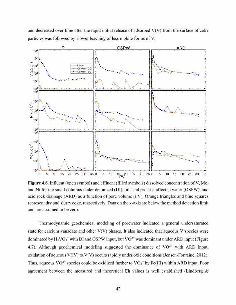
42
and decreased over time after the rapid initial release of adsorbed V(V) from the surface of coke
particles was followed by slower leaching of less mobile forms of V.
Figure 4.6. Influent (open symbol) and effluent (filled symbols) dissolved concentration of V, Mo,
and Ni for the small columns under deionized (DI), oil sand process-affected water (OSPW), and
acid rock drainage (ARD) as a function of pore volume (PV). Orange triangles and blue squares
represent dry and slurry coke, respectively. Data on the x-axis are below the method detection limit
and are assumed to be zero.
Thermodynamic geochemical modeling of porewater indicated a general undersaturated
state for calcium vanadate and other V(V) phases. It also indicated that aqueous V species were
dominated by H2VO4− with DI and OSPW input, but VO2+ was dominant under ARD input (Figure
4.7). Although geochemical modeling suggested the dominance of VO2+ with ARD input,
oxidation of aqueous V(IV) to V(V) occurs rapidly under oxic conditions (Jensen-Fontaine, 2012).
Thus, aqueous VO2+ species could be oxidized further to VO2+ by Fe(III) within ARD input. Poor
agreement between the measured and theoretical Eh values is well established (Lindberg &

43
Runnells, 1984), and a slight decrease in input Eh values (±50 mV) shifted the model prediction
to Fe(III) or Fe(II) as the dominant Fe oxidation state. The V oxidation state is sensitive to Eh
values, especially with ARD input, since a slight change in Eh shifts the model prediction to V(V)
or V(IV) as the dominant form. Based on dissolved V concentrations and geochemical modeling,
poly-nuclear V species were not expected to form (Figure 4.7).
Figure 4.7. Pourbaix (Eh–pH) diagram for vanadium (top) and a predominance diagram showing
aqueous V(V) speciation as a function of pH and total V concentration (bottom). All V aqueous
species were assumed to be V(V) in the second figure. Squares, triangles, and circles represent
data points for deionized (DI), oil sand process-affected water (OSPW), and acid rock drainage
(ARD), respectively. Filled symbols represent slurry coke and empty symbols represent dry coke.
Variation in dissolved V concentrations in the column effluent under different water input
compositions could be a result of pH-dependent sorption of V(V) onto the coke surface, or
oxidation and dissolution of V complexes. According to porewater pH and pHPZC for coke (6.7–
7.2), the coke had a net positive surface charge with DI and ARD (pH < pHPZC), but the surface
charge was negative with OSPW (pH > pHPZC). Therefore, the high ionic strength of ARD (I ⁓0.2)

44
and OSPW (I ⁓0.05), in addition to unfavorable conditions for V(V) adsorption on the coke surface
including net surface charge and dominance of VO2+ (or VO2+) or H2VO4
−, mobilized V from the
coke surface. Meanwhile, V mobility was limited and controlled by the adsorption of aqueous
H2VO4− with DI input.
Cumulative V release calculations indicate that V leaching occurred under all water input
compositions, however the leaching efficiency (the proportion of total leached to the bulk
concentration) was relatively low, with a maximum 0.90% (12800 µg kg−1) observed for slurry
coke under ARD (Table 4.3, Appendix H). This is attributed to the large portion of V associated
with porphyrin complexes (Nesbitt et al., 2017; Nesbitt and Lindsay, 2017), which are stable and
resistant to weathering (Lewan & Maynard, 1982; Zuliani et al., 2016). Slurry coke exhibited a
higher leaching potential than dry coke with 1.27 µg kg−1 compared with 5030 µg kg−1 with DI
input, 70.5 µg kg−1 compared with 10100 µg kg−1 with OSPW input, and 3290 µg kg−1 compared
with 12800 µg kg−1 with ARD (Table 4.3). In addition, over 50% of the cumulative V release
occurred during the first five PV in experiments using dry and slurry coke with DI and ARD, and
slurry coke with OSPW, representing the initial release of adsorbed V(V). While only 36% of
cumulative V was released from the dry coke with OSPW given the slow leaching of rate of V
(Figure 4.8, Appendix H).
Table 4.3. Cumulative mass release per kg of fluid petroleum coke for the small columns.
Elements DIa (μg) OSPWb (μg) ARDc (μg)
DCd SCe DC SC DC SC
V 1.27 5030 70.5 10100 3290 12800
Ni 1170 1330 760 651 2110 3550
Mo 3.82 514 276 869 758 610
aDI: Deionized water
bOSPW: Oil sand process-affected water
cARD: Acid rock drainage
dDC: Dry coke
eSC: Slurry coke

45
Figure 4.8. Cumulative mass release per kg of coke under deionized (DI), oil sand process-affected
water (OSPW), and acid rock drainage (ARD) as function of pore volume (PV). Orange lines
represent the dry coke; blue lines represent slurry coke.
4.3.1.2. Nickel
Nickel concentrations in column effluent with DI input were 0–1520 μg L−1 for dry coke and
9.70–655 μg L−1 for slurry coke, with OSPW input they were 0–929 μg L−1 for dry coke and 10.5–
113 μg L−1 for slurry coke, and for ARD input they were 25.1–2600 μg L−1 for dry coke and 38.5–
8460 μg L−1 for slurry coke (Figure 4.6, Appendix G). Aqueous Ni concentrations followed a
general order of ARD > DI > OSPW and decreased over time with the rapid initial release of Ni
from the surface of coke particles followed by slower leaching of less mobile and available forms
of Ni.
Thermodynamic modeling indicated that with DI and OSPW input, Ni2+ was the dominant
aqueous Ni species making up over 45% of aqueous Ni, while NiSO40 and NiHCO3
+ accounted

46
for the rest (Figure 4.9). However, during DI input, the proportions of NiSO40 and NiHCO3
+
species decreased rapidly over three pore volumes and shifted completely to Ni2+ while SO42− and
HCO3− (alkalinity) decreased (Figure 4.4 and 4.5). Speciation of aqueous Ni during ARD input
showed that NiSO40 and Ni2+ accounted for approximately 50% of aqueous Ni. Geochemical
modeling showed that porewater was consistently undersaturated with respect to NiO(S), NiCO3(S),
and Ni(OH)2(S). Therefore, these phases do not control the dissolved aqueous Ni concentration.
Complexation of Ni with bicarbonate and sulfate forms non-ionic species (NiHCO3+, NiSO4
0)
which may increase Ni mobility and limit Ni sorption.
Figure 4.9. Pourbaix (Eh–pH) diagram for Ni. Squares, triangles, and circles represent data points
for deionized (DI), oil sand process-affected water (OSPW), and acid rock drainage (ARD),
respectively. Filled symbols represent data points for slurry coke and blank symbols represent dry
coke.
A significant negative correlation between pH values and dissolved Ni concentrations (r =
−0.25) and alkalinity values (r = −0.19) was observed, suggesting that pH-dependent precipitation–
dissolution and sorption reactions are the principal factors controlling Ni mobility and aqueous
concentrations within coke. A similar negative correlation value between pH values and Ni
concentrations was reported by Puttaswamy & Liber (2011) and Nesbitt et al. (2018). Coke showed
a positive net surface charge when porewater pH was less than pHPZC (6.7–7.2), therefore,
observing higher Ni concentrations in the column effluent during DI and ARD input compared
with OSPW could be explained by a net positive surface charge along with the presence of cationic
or non-ionic Ni species such as Ni2+, NiHCO3+, and NiSO4
0. Therefore, Ni had higher mobility

47
with DI and ARD, while Ni mobility was limited during OSPW because of adsorption of cationic
Ni species, including Ni2+ and NiHCO3+, on the coke surface.
Cumulative mass release calculations indicated that Ni had a higher leaching potential from
slurry than from dry coke with DI input (1330 µg kg−1 for slurry coke; 1170 µg kg−1 for dry coke),
OSPW input (650 µg kg−1 for slurry coke; 760 µg kg−1 for dry coke), and for ARD input (3550 µg
kg−1 for slurry coke; 2110 µg kg−1 for dry coke; Table 4.3). Although Ni leaching occurred during
all water input compositions, leaching efficiency was relatively low (<1%) to a maximum of 0.65%
(3550 µg) of total Ni observed for slurry coke during the ARD input (Table 4.3, Appendix H).
This result is attributed to large portion of Ni associated with porphyrin complexes (Nesbitt et al.,
2017, 2018), which are stable and resistant to weathering (Lewan & Maynard, 1982; Zuliani et al.,
2016). During DI and ARD inputs, approximately 60% of Ni leaching occurred during the first
five pore volumes for both dry and slurry coke as a rapid initial release of Ni phases. Under OSPW
input, around 90% of the Ni leaching from dry coke occurred during the first five pore volumes,
whereas only 33.6% of Ni was leached from slurry coke. Nickel leaching from slurry coke was
more gradual during OSPW input and required more volume (19 pore volumes) to reach 90% of
total Ni cumulative mass (Figure 4.8, Appendix H).
4.3.1.3. Molybdenum
Effluent Mo concentrations were 0–5.84 μg L−1 for dry coke and 0.58–500 μg L−1 for slurry
coke during DI input, 3.45–22.1 μg L−1 for dry coke and 4.55–147 μg L−1 for slurry coke during
OSPW input, and 21.3–408 μg L−1 for dry coke and 3.41 to 102 μg L−1 for slurry coke during ARD
input (Figure 4.6, Appendix G). Aqueous Mo concentrations decreased over time after the rapid
initial release of Mo from the coke surface was followed by slower leaching of less mobile forms
of Mo. Dissolved Mo concentrations within the column effluent followed a general order of ARD
> OSPW > DI.
Geochemical modeling indicated that MoO42− was the dominant aqueous Mo species during
DI and OSPW input for both dry and slurry coke. In contrast, H2MoO40 was the dominant aqueous
Mo species under ARD input for both dry and slurry coke (Figure 4.10). Thermodynamic modeling
showed a general undersaturated state with respect to metal molybdates such as NiMoO4 and
CaMoO4, which are likely to dissolve if present. Consequently, the precipitation of Mo phases
does not control Mo mobility in this system. Because of the low concentration of aqueous Mo
observed within the system, poly-nuclear species are not expected to form (Figure 4.10).

48
Figure 4.10. Pourbaix (Eh–pH) diagram (top) and Log concentration vs. pH for Mo(VI) (bottom).
Squares, triangles, and circles represent data points for deionized (DI), oil sand process-affected
water (OSPW), and acid rock drainage (ARD), respectively. Filled symbols represent data points
for slurry coke; blank symbols represent data points for dry coke.
Robertson et al. (2019) reported that dissolved Mo concentrations and mobility is controlled
by outer-sphere MoO42− complexation. Surface complexation of MoO4
2− is greatest when
porewater pH is less than the pHPZC (6.7 to 7.2, Appendix E) and the net surface charge is positive.
Despite these conditions existing during DI and ARD input, complexation was limited during ARD
input when H2MoO40 was predicted to be the dominant aqueous Mo species. An increase in
effluent Mo concentrations for the slurry coke during ARD input within the first pore volume was
observed (Figure 4.6). This increase could be explained by the initial presence of HMoO4− species
(up to 30% of aqueous Mo species based on thermodynamic modeling), and net positive surface
(pH < pHPZC) of coke. Thus, possible attenuation by surface complexation could limit Mo mobility

49
in the beginning, while the proportion of HMoO4− species dropped rapidly to less than 5% after
the first pore volume; therefore, Mo mobility was increased over the first pore volume resulting in
higher Mo concentrations in the column effluent.
Iron-(hydr)oxides, pyrite, clays, and organic matter are phases within coke that could
potentially adsorb MoO42− (Goldberg et al., 1996; Bostick et al., 2003; Gustafsson & Tiberg,
2015). Their presence in coke was observed with EMPA and bulk geochemistry analyses (Figure
4.3) and also reported previously by Kessler & Hendry (2006) and Nesbitt et al. (2017). During
DI input, these phases could adsorb MoO42−, while under increased pH and ionic strength the
potential to adsorb MoO42− decreases (Goldberg & Forster, 1998; Gustafsson & Tiberg, 2015).
Therefore, unfavorable attenuation of aqueous Mo species, the high ionic strength of ARD (I ⁓
0.2) and OSPW (I ⁓ 0.05), and the presence of some anions such as Cl− and HCO3− in OSPW that
compete with MoO42− for complexation on the coke surface resulted in higher leaching and
mobility of Mo during OSPW and ARD input. Meanwhile, the low ionic strength of DI (I < 0.01)
and attenuation of MoO42− led to low Mo concentrations and leaching (Figure 4.6, Table 4.3). This
result is consistent with the significant positive correlation between dissolved Mo concentration
and alkalinity (r = 0.61) and EC (r = 0.22) under OSPW and ARD inputs. Also, Puttaswamy &
Liber (2012) reported an increase in Mo mobility in the presence of Cl− and HCO3−.
Molybdenum leaching occurred under all water input compositions; however, leaching
efficiency was relatively low for all geochemical conditions (Appendix H). Slurry coke had a
higher leaching potential compared with dry coke (3.82 vs. 514 µg kg−1 during DI, 276 vs. 780 µg
kg−1 under OSPW, and 758 vs. 610 µg kg−1 during ARD inputs; Table 4.3). During DI and OSPW
input, over 50% of Mo leaching occurred during the first five pore volumes for both dry and slurry
coke as a rapid initial release of Mo phases occurred (Figure 4.8). Under ARD input, leaching was
more gradual, and after five pore volumes only 40.4% and 33.5% of leaching occurred for dry and
slurry coke, respectively. Molybdenum leaching during ARD input required more time to reach
90% of Mo cumulative mass release, requiring 19.8 pore volumes and 13.8 pore volumes for dry
and slurry coke, respectively (Figure 4.8, Appendix H).
4.3.2. Transport Parameters
According to tracer test results and obtained breakthrough curves for the dry coke during DI
input (Figure 4.11), the average linear pore water velocity and the dispersivity coefficient were
3.88 × 10⁻⁷ m s−1 and 0.166 cm, respectively (Table 4.4). However, for columns under ARD input,

50
no Br− was detected within the effluent because of the net positive surface and adsorption of Br−.
Also, because of the similarity in flow rates, packed mass in the columns, and the PSD of dry coke
and slurry coke for the small columns, the porewater velocity and dispersivity coefficient were
similar among the columns. Therefore, the average linear pore water velocity and the dispersivity
coefficient were calculated and applied to the small columns (Table 4.4). The residence time of
the column was 6.64 d (Table 4.4); this is a particularly important parameter in hydrogeochemical
systems because it affects kinetically controlled reactions and is directly linked to cumulative mass
discharge.
Figure 4.11. Breakthrough curve for dry coke during DI input (black line). Error bars represent
the electrode ±2.5% electrode sensitivity. Red dashed lines indicate the lower and higher 95%
confidence.
Table 4.4. Calculated hydraulic parameters for dry coke during DI input.
Parameter Units Value
Average linear velocity m s−1 3.88 × 10⁻⁷
Dispersivity cm 0.166
PVa L 0.33
aPV: pore volume
51
4.4. Large Column
4.4.1. Aqueous Geochemistry
The pH of influent solutions remained relatively constant throughout the experiment with
the median value 7.40 for DI, 8.70 for synthetic OSPW, 8.90 for field OSPW, and 2.10 for ARD.
The effluent pH ranged from 4.62–5.53 during DI input, 5.88–6.80 for synthetic OSPW input, and
6.6–7.10 for field OSPW input, which was a decrease compared to the influent pH (Figure 4.12).
The pH reduction under DI and OSPW influent (both synthetic and field), along with the presence
of Fe and S in the column effluent (Figure 4.13), is indicative of acid generation via Fe-S–bearing
phase oxidation (i.e., pyrite). Oxidation of Fe-S phases generates protons and releases S, and the
presence of Fe-S phases was observed within the coke matrix in the EMPA-EDX spectra (Figure
4.3) and reported previously by Kessler & Hendry (2006). Also, elevated concentrations of Ca,
Mg, Sr, and Ba in the column effluent (Appendix G) in addition to the significant positive
correlation of Sr with Ca (r = 0.98), Mg (r = 0.84), and Ba (r = 0.47) indicate carbonate dissolution.
The pH decrease within the system could lead to carbonate dissolution and mobilize these
elements. Although pH differences between the influent and effluent under ARD input were not
significant and generally were similar, a slightly higher pH (2.40–2.70) was observed in the
effluent during the first pore volume (Figure 4.12).
The influent EC and alkalinity of all solutions was relatively consistent during the
experiment. The median EC for the influent was 15.30 µS cm−1 for DI, 4.82 mS cm−1 for synthetic
OSPW, and 4.97 mS cm−1 for OSPW. The median EC for the ARD solution used throughout the
experiment was 8.94 mS cm−1 (Figure 4.12). The median value for influent alkalinity was
9.96 mg L−1 (as CaCO3) for DI, 714 mg L−1 for synthetic OSPW, and 920 mg L−1 for field OSPW.
Alkalinity could not be measured for the ARD solution because the influent and porewater pH are
less than the pH of the bromocresol green methyl indicator (Figure 4.12).
The EC and alkalinity of the effluent from DI input decreased rapidly from 1350 to
97.0 µS cm−1 and from 84.0 to 38.0 mg L−1 (as CaCO3) after three pore volumes (Figure 4.12).
The EC decreased from 1350 to 53.0 µS cm−1 under DI input, whereas it ranged from 4 to 5.10
mS cm−1 under OSPW input and 6.40 to 9.60 mS cm−1 under ARD input (Figure 4.12). In addition,
the alkalinity ranged from 21.8 to 91 mg L−1 (as CaCO3) under DI input, while it ranged from 485
to 934 mg L−1 (as CaCO3) under OSPW input. During OSPW (both synthetic and field) and ARD
input, the differences between column influent and effluent EC values were not measurable (Figure
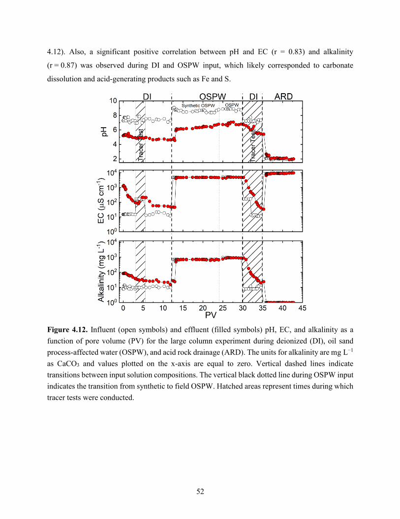
52
4.12). Also, a significant positive correlation between pH and EC (r = 0.83) and alkalinity
(r = 0.87) was observed during DI and OSPW input, which likely corresponded to carbonate
dissolution and acid-generating products such as Fe and S.
Figure 4.12. Influent (open symbols) and effluent (filled symbols) pH, EC, and alkalinity as a
function of pore volume (PV) for the large column experiment during deionized (DI), oil sand
process-affected water (OSPW), and acid rock drainage (ARD). The units for alkalinity are mg L−1
as CaCO3 and values plotted on the x-axis are equal to zero. Vertical dashed lines indicate
transitions between input solution compositions. The vertical black dotted line during OSPW input
indicates the transition from synthetic to field OSPW. Hatched areas represent times during which
tracer tests were conducted.
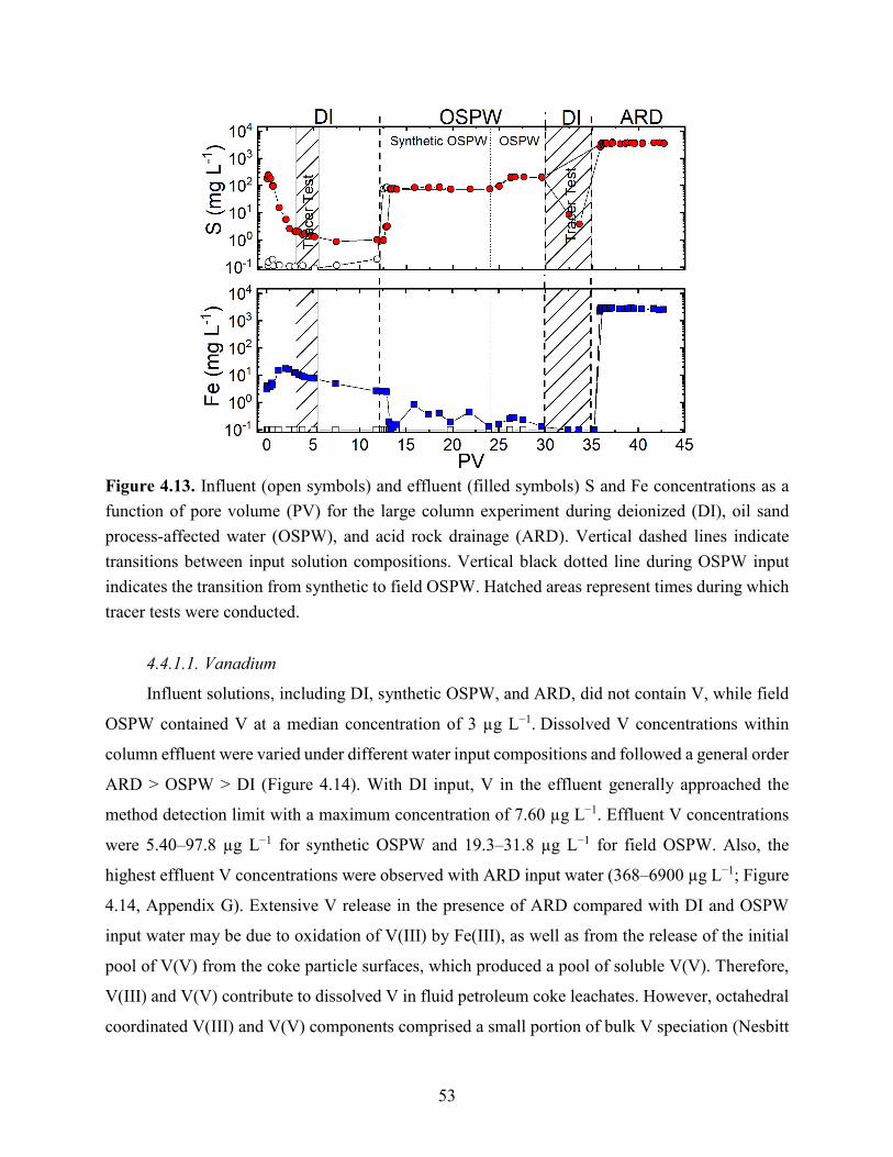
53
Figure 4.13. Influent (open symbols) and effluent (filled symbols) S and Fe concentrations as a
function of pore volume (PV) for the large column experiment during deionized (DI), oil sand
process-affected water (OSPW), and acid rock drainage (ARD). Vertical dashed lines indicate
transitions between input solution compositions. Vertical black dotted line during OSPW input
indicates the transition from synthetic to field OSPW. Hatched areas represent times during which
tracer tests were conducted.
4.4.1.1. Vanadium
Influent solutions, including DI, synthetic OSPW, and ARD, did not contain V, while field
OSPW contained V at a median concentration of 3 µg L−1. Dissolved V concentrations within
column effluent were varied under different water input compositions and followed a general order
ARD > OSPW > DI (Figure 4.14). With DI input, V in the effluent generally approached the
method detection limit with a maximum concentration of 7.60 µg L−1. Effluent V concentrations
were 5.40–97.8 µg L−1 for synthetic OSPW and 19.3–31.8 µg L−1 for field OSPW. Also, the
highest effluent V concentrations were observed with ARD input water (368–6900 µg L−1; Figure
4.14, Appendix G). Extensive V release in the presence of ARD compared with DI and OSPW
input water may be due to oxidation of V(III) by Fe(III), as well as from the release of the initial
pool of V(V) from the coke particle surfaces, which produced a pool of soluble V(V). Therefore,
V(III) and V(V) contribute to dissolved V in fluid petroleum coke leachates. However, octahedral
coordinated V(III) and V(V) components comprised a small portion of bulk V speciation (Nesbitt

54
& Lindsay, 2017). These findings suggest that even if V leaching by DI and OSPW becomes
limited, a switch to acidic conditions could promote additional leaching. Aqueous V
concentrations decreased over time during input of synthetic OSPW and ARD as the rapid initial
release of adsorbed V(V) from the coke particle surfaces was followed by slower leaching of less
mobile and available V forms. Vanadium concentrations were significantly correlated with pH
values (r = −0.61) and EC values (r = 0.51), suggesting that the high ionic strength of OSPW
(I ⁓ 0.05) and ARD (I ⁓ 0.2) and the low pH of ARD (pH ⁓ 2) resulted in higher V release.
Figure 4.14. Influent (open symbols) and effluent (filled symbols) V, Mo, and Ni aqueous
concentrations as a function of pore volume for the large column experiment during deionized
(DI), oil sand process-affected water (OSPW), and acid rock drainage (ARD). All concentrations
are in μg L−1 and values plotted on x-axis are below the method detection limit. Vertical dashed
lines indicate a transition between input solution compositions. Vertical black dotted line in the
OSPW phase indicates the transition from synthetic to field OSPW. Hatched areas represent times
during which tracer tests were conducted.

55
Based on thermodynamic modeling, H2VO4− was the dominant aqueous V species in the
column effluent during DI and OSPW input, whereas VO+2 and VO2+ were the dominant species
during ARD input (Figure 4.15). However, oxidation of aqueous V(IV) to V(V) occurs rapidly
under oxic conditions (Jensen-Fontaine, 2012). Therefore, aqueous VO+2 present during ARD
input could be oxidized further to VO2+. Dissolved V(IV) and V(V) within the coke leachate have
been reported previously by Li et al. (2007). Also, thermodynamic modeling showed that
porewater was consistently undersaturated with respect to calcium vanadate and other V(V)
phases. Due to the low concentration of V (V < 10−3.87 M), poly-nuclear species are not expected
to form (Figure 4.15). Also, poor agreement between the measured and theoretical Eh values is
well established (Lindberg & Runnells, 1984) and a slight decrease in the input Eh values (±50
mV) shifted the model prediction to Fe(III)/Fe(II) as the dominant Fe oxidation state.
Figure 4.15. Pourbaix (Eh–pH) diagram for vanadium (top) and predominance diagram showing
aqueous V(V) speciation as a function of pH and total V concentration (bottom). Blue squares, red
triangles, and orange circles represent data points for during deionized (DI), oil sand process-
affected water (OSPW), and acid rock drainage (ARD), respectively.
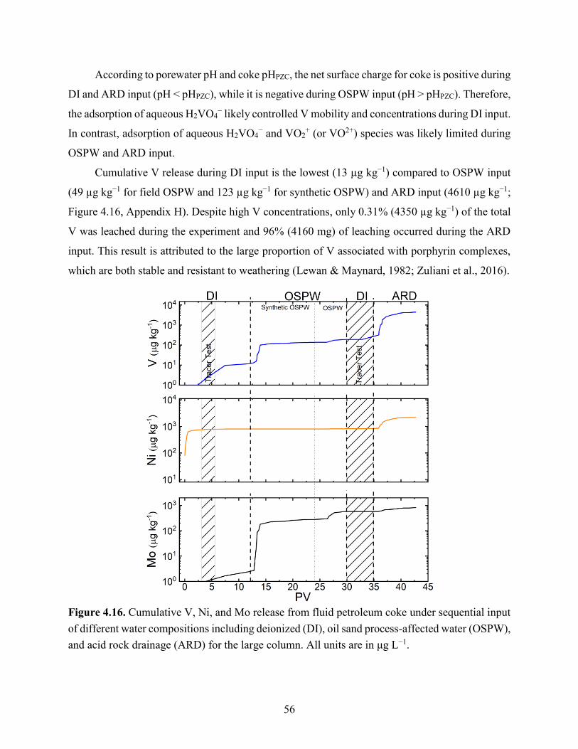
56
According to porewater pH and coke pHPZC, the net surface charge for coke is positive during
DI and ARD input (pH < pHPZC), while it is negative during OSPW input (pH > pHPZC). Therefore,
the adsorption of aqueous H2VO4− likely controlled V mobility and concentrations during DI input.
In contrast, adsorption of aqueous H2VO4− and VO2
+ (or VO2+) species was likely limited during
OSPW and ARD input.
Cumulative V release during DI input is the lowest (13 µg kg−1) compared to OSPW input
(49 µg kg−1 for field OSPW and 123 µg kg−1 for synthetic OSPW) and ARD input (4610 µg kg−1;
Figure 4.16, Appendix H). Despite high V concentrations, only 0.31% (4350 µg kg−1) of the total
V was leached during the experiment and 96% (4160 mg) of leaching occurred during the ARD
input. This result is attributed to the large proportion of V associated with porphyrin complexes,
which are both stable and resistant to weathering (Lewan & Maynard, 1982; Zuliani et al., 2016).
Figure 4.16. Cumulative V, Ni, and Mo release from fluid petroleum coke under sequential input
of different water compositions including deionized (DI), oil sand process-affected water (OSPW),
and acid rock drainage (ARD) for the large column. All units are in μg L−1.

57
4.4.1.2. Nickel
Column influent solutions, including DI, synthetic OSPW, and ARD did not contain Ni,
while field OSPW contained Ni at a median concentration of 7.86 μg L−1. Dissolved Ni
concentrations within the column effluent were varied for different water compositions and
followed a general order ARD > DI > OSPW (Figure 4.14). Effluent Ni concentrations during DI
input were 7.80–1880 μg L−1 compared with 62.4–2300 μg L−1 during ARD input. Porewater Ni
concentrations were close to the method detection limit under OSPW input, with a maximum
concentration of 5.58 μg L−1 during field OSPW input (Figure 4.14, Appendix G). Aqueous Ni
concentrations decreased over time during ARD and DI input as the rapid initial release of Ni
phases from the coke particle surface was followed by slower leaching of less mobile and available
inorganic Ni forms including Ni(II)-sulfide and Ni(II)-oxide.
Geochemical modeling indicated that Ni2+ accounted for 50 to 90% of dissolved Ni within
column effluent under ARD and DI input, while NiSO40 comprised the remainder (Figure 4.17).
Thermodynamic modeling also showed that Ni2+ accounted for ⁓50% of dissolved Ni in the
column effluent under field OSPW input, whereas NiSO40 and NiHCO3
+ comprised ⁓10% and
⁓30%, respectively. Complexation of Ni with carbonate and sulfate forms non-ionic species
(NiCO30, NiSO4
0) which may increase Ni mobility and limit Ni sorption. Thermodynamic
modeling suggested a general undersaturated state with respect to NiO(s), NiCO3(s), and Ni(OH)2(s)
which means these phases were not principal controls on dissolved Ni concentrations.
Figure 4.17. Pourbaix (Eh–pH) diagram for Ni. Blue squares, red triangles, and orange circles
represent data points for deionized (DI), oil sand process-affected water (OSPW), and acid rock
drainage (ARD), respectively.

58
A significant negative correlation between Ni concentrations and pH values (r = −0.38) and
alkalinity values (r = −0.44) was observed, which suggests that pH-dependent precipitation–
dissolution and sorption reactions are principal controls on Ni mobility during the experiment. A
similar negative correlation between aqueous Ni concentrations and pH has been reported
previously by Puttaswamy & Liber (2011) and Nesbitt et al. (2018). Considering the porewater pH
and pHPZC for coke, the net surface charge of coke is negative during OSPW input, while it is
positive under DI and ARD input. The net positive surface charge and dominance of cationic or
non-ionic species (Ni2+ and NiSO40) during DI and ARD input enhanced Ni mobility. Ni mobility
was limited during OSPW input due to the net negative surface charge and dominance of Ni2+ and
NiHCO3+ species. Adsorption of these Ni species onto the coke surface could explain why a lower
Ni concentration was observed in the effluent compared with influent during field OSPW input
(Figure 4.14).
Nickel mobility under synthetic OSPW input was limited, with a concentration equal to zero
in the effluent, while Ni was attenuated within the system during field OSPW input, resulting in a
negative cumulative release. Although Ni leaching occurred during DI and ARD input, only 0.40%
(2160 µg kg−1) of total Ni was leached during the experiment, with ⁓37% (800 µg kg−1) and ⁓ 63%
(1360 µg kg−1) leached during DI and ARD input, respectively (Appendix H). This result is
attributed to the large proportion of Ni associated with porphyrin complexes, which are both stable
and resistant to weathering (Lewan & Maynard, 1982; Zuliani et al., 2016).
4.4.1.3. Molybdenum
Column influent solutions, including DI, synthetic OSPW, and ARD, did not contain Mo,
while field OSPW contained Mo at a median concentration of 133 μg L−1. Dissolved Mo
concentrations within the column effluent were varied for different water compositions and
followed a general order OSPW > ARD > DI (Figure 4.14). Effluent Mo concentrations were 13–
574 μg L−1 for synthetic OSPW input compared with 57.5–153 μg L−1 for field OSPW input. Also,
Mo concentrations in the effluent were 35.5–160 μg L−1 during ARD input. Porewater Mo
concentrations approached the method detection limit during DI input to a maximum concentration
of 3.80 μg L−1 (Figure 4.14, Appendix G). Aqueous Mo concentrations decreased over time during
OSPW and ARD input, as the rapid initial release of Mo phases at the coke particle surfaces was
followed by slower leaching of less mobile and available outer-sphere Mo forms.

59
Thermodynamic modeling suggested that MoO42− was the dominant aqueous Mo species
under DI and OSPW input, while H2MoO40 was the dominant species in the effluent during ARD
input (Figure 4.18). Geochemical modeling indicated a general undersaturated state with respect
to metal molybdates, which are likely to dissolve if they are present. In addition, due to the low
dissolved Mo concentrations, poly-nuclear species were not expected to form (Figure 4.18).
Figure 4.18. Pourbaix (Eh–pH) diagram for vanadium (top) and predominance diagram showing
Mo(VI) aqueous speciation as function of pH and concentration (bottom). Blue squares, red
triangles, and orange circles represent data points for deionized (DI), oil sand process-affected
water (OSPW), and acid rock drainage (ARD), respectively.
Robertson et al. (2019) reported that outer-sphere complexation of MoO42− influences
dissolved Mo concentrations and mobility in coke deposits. Surface complexation of MoO42− is
greatest when pore water pH is less than pHPZC (6.7 to 7.2, Appendix E) and the net surface charge
is positive. Although these conditions existed during DI and ARD input, complexation was likely
limited during ARD input when H2MoO40 was predicted to be the dominant aqueous Mo species.

60
Therefore, it is unfavorable for H2MoO40 and MoO4
2− to be attenuated under OSPW and ARD
input, while MoO42− was attenuated during DI input via outer-sphere complexes.
The presence of Fe-(hydr)oxides, pyrite, clays, and organic matter within coke particles was
observed by EMPA and bulk geochemistry analyses, and their presence was also previously
reported by Kessler & Hendry (2006) and Nesbitt et al. (2017). These phases can potentially adsorb
MoO42− under mildly acidic conditions (⁓pH 3–6; Goldberg et al., 1996; Bostick et al., 2003;
Gustafsson & Tiberg, 2015). During DI input, these phases could adsorb MoO42−, while the
increased pH and ionic strength decreased their adsorption capacity (Goldberg & Forster, 1998;
Gustafsson & Tiberg, 2015); therefore, MoO42− attenuation was unlikely to occur under OSPW
and ARD input. A significant positive correlation between dissolved Mo concentrations and EC (r
= 0.26) and alkalinity (r = 0.36) was observed, suggested that the leachable portion of Mo is in
outer-sphere MoO42− complexes. Additionally, Cl− and HCO3
− would compete with MoO42− for
sorption on the coke surface, therefore their presence within solution would increase Mo mobility
(Puttaswamy & Liber, 2012), which is consistent with the higher mobility of Mo observed during
OSPW input compared to DI input (Figure 4.14). The high ionic strength of ARD (I ⁓ 0.2) and
OSPW (I ⁓ 0.05) and the presence of some anions such as Cl− and HCO3− within the OSPW phases
stimulates desorption of MoO42− outer-sphere complexes at the coke surface.
Cumulative Mo release during DI and field OSPW inputs were the lowest, at 4 and 2 µg
kg−1, respectively. Most Mo leaching occurred under synthetic OSPW and ARD input, at 280 and
235 µg kg−1, respectively (Figure 4.16, Appendix H). However, only 0.69% (520 µg kg−1) of the
total Mo within the bulk coke was leached during the experiment. This result is attributed to the
large portion of Mo associated with Mo(IV) disulfide, which is strongly resistant to oxidation
(Lindsay et al., 2015; Plumlee, 1999).
4.4.2. Geophysical inversion and forward modeling results
4.4.2.1. Inversion modeling of resistivity
The apparent resistivity declined as a solution containing Br−, with a higher EC (165.5 µS
cm−1), was passed through the column, while the decay part exhibited an increase in apparent
resistivity as the saturated column was flushed with DI having lower EC (15.5 µS cm−1) (Figure
4.19). The average linear pore water velocities for the injection and decay portions of the first
tracer test were 6.98 ± 0.15 × 10⁻⁷ and 8.33 ± 0.27 × 10⁻⁷ m s−1, and were generally consistent
(Table 4.5).

61
Figure 4.19. Apparent resistivity as function of time (left) and linear regression of mid-point
(right) which define the average linear velocity for the first tracer. This includes the injection of
the tracer (top) and decay of the first tracer (bottom). Electrodes were configured in a ring position,
with R1 to R8 placed from the bottom to top of the column.
Table 4.5. Average linear velocities for the large column, measured based on mid-point theory for
the first tracer test including injection and decay.
Array configuration Units Injection Decay
Ring m s−1 7.26× 10⁻⁷ 7.87× 10⁻⁷
Lateral A-Wenner m s−1 6.92× 10⁻⁷ 8.43× 10⁻⁷
Lateral B-Wenner m s−1 6.99× 10⁻⁷ 8.44× 10⁻⁷
Lateral C-Wenner m s−1 6.83× 10⁻⁷ 8.22× 10⁻⁷
Lateral D-Wenner m s−1 6.90× 10⁻⁷ 8.68× 10⁻⁷
The line intercept for linear regression in figure 4.19 shows the point of injection (column
inlet port) in decay part of tracer; first electrode is located at 6 cm from the bottom of the column.

62
However since salt is released during the injection part of tracer test, the line intercept for the
injection part became irrelevant.
4.4.2.2. Forward modeling of resistivity
The forward modeling using measured hydrodynamic parameters from the tracer test, and
reaction rates for individual species (fitting the output concentration from the model with measured
aqueous concentration, Appendix A) inside COMSOL Multiphysics was calculated for all rings
(1-D). Since the measured apparent resistivity is not associated with a point, rather an average of
adjacent region to electrodes, the calculated apparent resistivity ±2.5 cm from the ring is also
considered. Results were in good agreement with measured values (Figures 4.13 and 4.14).
Calculated apparent resistivity from forward modeling were in good agreement with measured
apparent resistivity.
Figure 4.20. Forward modeling results for the first four rings (apparent resistivity vs. time) during
the first tracer test. The black line is the measured apparent resistivity associated with the ring
positions. Red, blue, and orange lines are the calculated apparent resistivity for that specific level
±2.5 cm.

63
Figure 4.21. Forward modeling results for the first four rings (apparent resistivity vs. time) during
the first tracer test (Decay). The black line is the measured apparent resistivity associated with the
ring positions. Red, blue, and orange lines are the calculated apparent resistivity for that specific
level ±2.5 cm.
4.4.3. Transport properties
According to tracer test results and obtained breakthrough curves for the large column
(Figure 4.22), the average linear pore water velocity and the dispersivity coefficients were 6.96 ±
0.163 × 10⁻⁷ m s−1 and 0.5763 ± 0.1661 cm, respectively (Table 4.6, Appendix I). Due to Na+
interference with the Br− electrode during the injection part of the second tracer test, which flushed
residual OSPW containing up to 1100 mg L−1 Na+ (Appendix G), the associated breakthrough
curve was noisy and was removed from our interpretation. In addition, the residence time of the
column was 11.02 ± 0.20 d (Table 4.6), which is a particularly important parameter in
hydrogeochemical systems because it affects kinetically controlled reactions and is directly linked
to cumulative mass discharge.

64
Figure 4.22. Breakthrough curve for the large column as a function of time (black line). Error bars
represent the electrode ±2.5% electrode sensitivity. Red dashed lines indicate the lower and higher
95% confidence.
Table 4.6. Calculated hydraulic parameters for the large column including first tracer test injection
part (A1), decay part (A2), and second tracer test-decay part (B2).
Parameter Units A1 A2 B2
Average linear velocity (×10−7) m s−1 6.86 7.19 6.83
Dispersivity cm 0.470 0.448 0.811
PVa L 5.29 5.17 5.40
aPV: pore volume

65
CHAPTER 5: CONCLUSIONS
The objectives of this research were to (i) investigate metal leaching (V, Mo, and Ni) from
fluid petroleum coke under the geochemical conditions existing in locations where coke might be
stored or used in the mine closure landscape, (ii) examine leaching efficiency and leaching
behavior over time, and (iii) establish forward and inverse geophysical modeling to evaluate
column transport properties. These objectives were addressed by a series of leaching experiments
under water compositions (meteoric water, OSPW, and ARD) that may interact with petroleum
coke at mine closure, and by linking geochemical factors to metal (V, Mo, and Ni) mobility.
This study concluded that V, Mo, and Ni are contaminants of potential concern within these
closure systems. Leaching of V and Mo during ARD and OSPW input was enhanced by oxic
conditions and/or high ionic strength of the solutions along with limited sorption. In the presence
of meteoric water, sorption attenuated V and Mo within the coke leachates. High net positive
surface charge of coke particles during ARD input along with the presence of V and Mo in their
cationic states (VO2+/VO2+ and H2MoO4
0) limited sorption, and therefore increased the mobility
of these metals. The high ionic strength of OSPW promoted desorption of Mo(VI) from outer-
sphere surface complexes. Finally, we attributed enhanced Ni leaching in the presence of meteoric
water and ARD to the limited potential for sorption and to the enhanced solubility of the hydroxide
or carbonate phases. The findings of this study complement those of earlier studies by Kessler and
Hendry (2006), Nesbitt (2016), and Swerhone (2018), and suggest that even if leaching in the
presence of meteoritic water is limited, switching to acidic conditions (by encountering ARD
water) could result in abundant V, Ni, and Mo leaching. The results from this research study can
be used to optimize mine closure design with respect to metal leaching and mobility.
Although metal leaching from fluid petroleum coke occurs through interactions with
different water compositions, leaching efficiency was generally low with less than 1% of bulk V,
Ni, and Mo concentrations leached. This is consistent with previous research by Kessler and
Hendry (2006) and Nesbitt (2016) that show low metal leaching rates from fluid petroleum coke.
The solid-phase fraction that hosts readily leachable metals is either volumetrically small, or the
coke grains contain these metals in a way that is largely inaccessible to porewater. Also, more
fractures, broken pieces, and particle attachment were observed in slurry coke compared with dry

66
coke, which could explain why slurry coke exhibited a higher leaching potential under all
geochemical conditions. In addition, the residual OSPW in slurry coke, which contains a small
amount of metals, could contribute to the apparent metal leaching and should be considered as
another source of metal leaching. Metal leaching (i.e, V, Ni, and Mo) decreased during the
experiment, which suggests that the leachable portion was limited.
Geophysical techniques (i.e., SP and RS) are helpful tools to study flow and transport
phenomena and could be used to characterize transport mechanisms in subsurface such as flow
pathways and velocity. These techniques provide necessary information to evaluate possible
contamination within subsurface since they are sensitive to variation in electrical properties such
as a possible leak from dam or tailings and will help manage, design, and optimize remediation
strategies. Using non-invasive and indirect methods with high sampling density in addition to
possible automated data acquisition makes geophysical methods important tools for subsurface
monitoring. However, these techniques cannot be used alone and they must be accompanied by
additional data from the other in situ tests (e.g., chemical analysis of pore water, pumping tests) to
verify the geoelectrical results.

67
REFERENCES
Adamson, A. (1973). Textbook of Physical Chemistry. Academic Press inc.
AER. (2015). Alberta’s Energy Reserves 2014 and Supply/Demand Outlook 2015– 2024. Alberta
Energy Regulator.
AER. (2019). ST: Alberta Mineable Oil Sands Plant Statistic (Calgary).
Ahmed, A. S., Jardani, A., Revil, A., & Dupont, J. P. (2016). Specific storage and hydraulic
conductivity tomography through the joint inversion of hydraulic heads and self-potential
data. Advances in Water Resources, 89, 80–90.
https://doi.org/10.1016/j.advwatres.2016.01.006
Alam, S., Cossio, M., Robinson, L., Wang, X., Kenney, J. P. L., Konhauser, K. O., MacKenzie,
M. D., Ok, Y. S., & Alessi, D. S. (2016). Removal of organic acids from water using
biochar and petroleum coke. Environmental Technology & Innovation, 6, 141–151.
https://doi.org/10.1016/j.eti.2016.08.005
Allison, J. D., Brown, D. S., & Novo-Gradac, K. J. (1991). MINTEQA2/PRODEFA2. A
geochemical assessment model for environmental systems U.S. EPA, Athens, GA 30613,
USA.
Archie, G. E. (1942). The Electrical Resistivity Log as an Aid in Determining Some Reservoir
Characteristics. Transactions of the AIME, 146(01), 54–62.
https://doi.org/10.2118/942054-G
Aureli, F., Ciardullo, S., Pagano, M., Raggi, A., & Cubadda, F. (2008). Speciation of
vanadium(IV) and (V) in mineral water by anion exchange liquid chromatography-
inductively coupled plasma mass spectrometry after EDTA complexation. Journal of
Analytical Atomic Spectrometry, 23(7), 1009–1016. https://doi.org/10.1039/B805234B
Baken, S., Larsson, M. A., Gustafsson, J. P., Cubadda, F., & Smolders, E. (2012). Ageing of
vanadium in soils and consequences for bioavailability. European Journal of Soil Science,
63(6), 839–847. https://doi.org/10.1111/j.1365-2389.2012.01491.x
Baker, L. F., Ciborowski, J. J. H., & MacKinnon, M. D. (2012). Petroleum coke and soft tailings
sediment in constructed wetlands may contribute to the uptake of trace metals by algae and
aquatic invertebrates. Science of The Total Environment, 414, 177–186.
https://doi.org/10.1016/j.scitotenv.2011.10.011

68
Binley, A., Cassiani, G., Middleton, R., & Winship, P. (2002). Vadose zone flow model
parameterisation using cross-borehole radar and resistivity imaging. Journal of Hydrology,
267(3), 147–159. https://doi.org/10.1016/S0022-1694(02)00146-4
Binley, A., Hubbard, S. S., Huisman, J. A., Revil, A., Robinson, D. A., Singha, K., & Slater, L.
D. (2015). The emergence of hydrogeophysics for improved understanding of subsurface
processes over multiple scales. Water Resources Research, 51(6), 3837–3866.
https://doi.org/10.1002/2015WR017016
Blackmore, D. P. T., Ellis, J., & Riley, P. J. (1996). Treatment of a vanadium-containing effluent
by adsorption/coprecipitation with iron oxyhydroxide. Water Research, 30(10), 2512–
2516. https://doi.org/10.1016/0043-1354(96)00080-2
Blanchard, P. E. R., Hayes, J. R., Grosvenor, A. P., Rowson, J., Hughes, K., & Brown, C.
(2015). Investigating the Geochemical Model for Molybdenum Mineralization in the JEB
Tailings Management Facility at McClean Lake, Saskatchewan: An X-ray Absorption
Spectroscopy Study. Environmental Science & Technology, 49(11), 6504–6509.
https://doi.org/10.1021/acs.est.5b00528
Bolève, A., Janod, F., Revil, A., Lafon, A., & Fry, J.-J. (2011). Localization and quantification of
leakages in dams using time-lapse self-potential measurements associated with salt tracer
injection. Journal of Hydrology, 403(3), 242–252.
https://doi.org/10.1016/j.jhydrol.2011.04.008
Borch, T., Kretzschmar, R., Kappler, A., Cappellen, P. V., Ginder-Vogel, M., Voegelin, A., &
Campbell, K. (2010). Biogeochemical Redox Processes and their Impact on Contaminant
Dynamics. Environmental Science & Technology, 44(1), 15–23.
https://doi.org/10.1021/es9026248
Bostick, B. C., Fendorf, S., & Helz, G. R. (2003). Differential Adsorption of Molybdate and
Tetrathiomolybdate on Pyrite (FeS2). Environmental Science & Technology, 37(2), 285–
291. https://doi.org/10.1021/es0257467
Buglyó, P., Crans, D. C., Nagy, E. M., Lindo, R. L., Yang, L., Smee, J. J., Jin, W., Chi, L.-H.,
Godzala, M. E., & Willsky, G. R. (2005). Aqueous Chemistry of the VanadiumIII (VIII)
and the VIII−Dipicolinate Systems and a Comparison of the Effect of Three Oxidation
States of Vanadium Compounds on Diabetic Hyperglycemia in Rats. Inorganic Chemistry,
44(15), 5416–5427. https://doi.org/10.1021/ic048331q
Burke, I. T., Mayes, W. M., Peacock, C. L., Brown, A. P., Jarvis, A. P., & Gruiz, K. (2012).
Speciation of Arsenic, Chromium, and Vanadium in Red Mud Samples from the Ajka Spill

69
Site, Hungary. Environmental Science & Technology, 46(6), 3085–3092.
https://doi.org/10.1021/es3003475
CAPP. (2018). Canadian Association of Petroleum Producers (CAPP). https://www.capp.ca
Chalaturnyk, R. J., Scott, J. D., & Özüm, B. (2002). Management of Oil Sands Tailings.
Petroleum Science and Technology, 20(9–10), 1025–1046. https://doi.org/10.1081/LFT-
120003695
Chung. (1996). Leachability of cokes from Syncrude stockpiles. March, 50–53.
Cilia, C. R. C. 1992-. (2018). Characterizing the Physical and Chemical Mass Transport of
Dissolved Salts in Layered Oil Sands Waste Undergoing Reclamation [Thesis, University
of Saskatchewan]. https://harvest.usask.ca/handle/10388/8323
Conlan, M. J. W., Mayer, K. U., Blaskovich, R., & Beckie, R. D. (2012). Solubility controls for
molybdenum in neutral rock drainage. Geochemistry: Exploration, Environment, Analysis,
12(1), 21–32. https://doi.org/10.1144/1467-7873/10-RA-043
Cordero, P. R. F., Bennett, R. M., Bautista, G. S., Aguilar, J. P. P., & Dedeles, G. R. (2015).
Degradation of Nickel Protoporphyrin Disodium and Vanadium Oxide Octaethylporphyrin
by Philippine Microbial Consortia. Bioremediation Journal, 19(2), 93–103.
https://doi.org/10.1080/10889868.2013.827616
Cruywagen, J. J. (1999). Protonation, Oligomerization, and Condensation Reactions of
Vanadate(V), Molybdate(vi), and Tungstate(vi). In A. G. Sykes (Ed.), Advances in
Inorganic Chemistry (Vol. 49, pp. 127–182). Academic Press.
https://doi.org/10.1016/S0898-8838(08)60270-6
Cruywagen, J. J., Heyns, J. B. B., & Westra, A. N. (1996). Protonation Equilibria of
Mononuclear Vanadate: Thermodynamic Evidence for the Expansion of the Coordination
Number in VO2+. Inorganic Chemistry, 35(6), 1556–1559. Scopus.
Das, A. K., Chakraborty, R., Cervera, M. L., & de la Guardia, M. (2007). A review on
molybdenum determination in solid geological samples. Talanta, 71(3), 987–1000.
https://doi.org/10.1016/j.talanta.2006.07.017
Dechaine, G. P., & Gray, M. R. (2010). Chemistry and Association of Vanadium Compounds in
Heavy Oil and Bitumen, and Implications for Their Selective Removal. Energy & Fuels,
24(5), 2795–2808. https://doi.org/10.1021/ef100173j
Elvingson, K., González Baró, A., & Pettersson, L. (1996). Speciation in Vanadium
Bioinorganic Systems. 2. An NMR, ESR, and Potentiometric Study of the Aqueous
70
H+−Vanadate−Maltol System. Inorganic Chemistry, 35(11), 3388–3393.
https://doi.org/10.1021/ic951195s
Essilfie-Dughan, J., Pickering, I. J., Hendry, M. J., George, G. N., & Kotzer, T. (2011).
Molybdenum Speciation in Uranium Mine Tailings Using X-Ray Absorption
Spectroscopy. Environmental Science & Technology, 45(2), 455–460.
https://doi.org/10.1021/es102954b
Fedorak, P. M., & Coy, D. L. (2006). Oil sands cokes affect microbial activities. Fuel, 85(12),
1642–1651. https://doi.org/10.1016/j.fuel.2006.02.015
Gamal El-Din, M., Fu, H., Wang, N., Chelme-Ayala, P., Pérez-Estrada, L., Drzewicz, P., Martin,
J. W., Zubot, W., & Smith, D. W. (2011). Naphthenic acids speciation and removal during
petroleum-coke adsorption and ozonation of oil sands process-affected water. Science of
The Total Environment, 409(23), 5119–5125.
https://doi.org/10.1016/j.scitotenv.2011.08.033
Genuchten, M. T. V. (1982). Analytical Solutions of the One-dimensional Convective-dispersive
Solute Transport Equation. U.S. Department of Agriculture, Agricultural Research
Service.
Gibson, J. J., Fennell, J., Birks, S. J., Yi, Y., Moncur, M. C., Hansen, B., & Jasechko, S. (2013).
Evidence of discharging saline formation water to the Athabasca River in the oil sands
mining region, northern Alberta. Canadian Journal of Earth Sciences, 50(12), 1244–1257.
https://doi.org/10.1139/cjes-2013-0027
Goldberg, S., & Forster, H. S. (1998). FACTORS AFFECTING MOLYBDENUM
ADSORPTION BY SOILS AND MINERALS. Soil Science, 163(2), 109–114.
Goldberg, S., Forster, H. S., & Godfrey, C. L. (1996). Molybdenum Adsorption on Oxides, Clay
Minerals, and Soils. Soil Science Society of America Journal, 60(2), 425–432.
https://doi.org/10.2136/sssaj1996.03615995006000020013x
Gray, M. R. (2015). Upgrading Oilsands bitumen and Heavy Oil (1st ed.). The University of
Alberta Press, Edmonto, Alberta.
Grosjean, E., Adam, P., Connan, J., & Albrecht, P. (2004). Effects of weathering on nickel and
vanadyl porphyrins of a Lower Toarcian shale of the Paris basin11Associate editor: G.
Logan. Geochimica et Cosmochimica Acta, 68(4), 789–804. https://doi.org/10.1016/S0016-
7037(03)00496-4
Gustafsson, J. P. (2018). Visual MINTEQ version.3.1 https://vminteq.lwr.kth.se/.
https://vminteq.lwr.kth.se/

71
Gustafsson, J. P. (2019). Vanadium geochemistry in the biogeosphere –speciation, solid-solution
interactions, and ecotoxicity. Applied Geochemistry, 102, 1–25.
https://doi.org/10.1016/j.apgeochem.2018.12.027
Gustafsson, J. P., & Tiberg, C. (2015). Molybdenum binding to soil constituents in acid soils: An
XAS and modelling study. Chemical Geology, 417, 279–288.
https://doi.org/10.1016/j.chemgeo.2015.10.016
Har, S. H. (1981). Characterization of oil sands fluid coke. ERA.
https://doi.org/10.7939/R3B853P38
Hein, F. J., & Cotterill, D. K. (2006). The Athabasca Oil Sands—A Regional Geological
Perspective, Fort McMurray Area, Alberta, Canada. Natural Resources Research, 15(2),
85–102. https://doi.org/10.1007/s11053-006-9015-4
Helz, G. R., Miller, C. V., Charnock, J. M., Mosselmans, J. F. W., Pattrick, R. A. D., Garner, C.
D., & Vaughan, D. J. (1996). Mechanism of molybdenum removal from the sea and its
concentration in black shales: EXAFS evidence. Geochimica et Cosmochimica Acta, 60,
3631–3642. https://doi.org/10.1016/0016-7037(96)00195-0
Holden, A. A., Mayer, K. U., & Ulrich, A. C. (2012). Evaluating methods for quantifying cation
exchange in mildly calcareous sediments in Northern Alberta. Applied Geochemistry,
27(12), 2511–2523.
Huang, J.-H., Huang, F., Evans, L., & Glasauer, S. (2015). Vanadium: Global (bio)geochemistry.
Chemical Geology, C(417), 68–89. https://doi.org/10.1016/j.chemgeo.2015.09.019
Hubbard, S., & Linde, N. (2011). Hydrogeophysics. In: Wilderer P (ed) Treatise on water
science, 1. Academic, Oxford, pp 401–434.
Huerta-Diaz, M. A., Tessier, A., & Carignan, R. (1998). Geochemistry of trace metals associated
with reduced sulfur in freshwater sediments. Applied Geochemistry, 13(2), 213–233.
https://doi.org/10.1016/S0883-2927(97)00060-7
Hummel, W., & Curti, E. (2003). Nickel Aqueous Speciation and Solubility at Ambient
Conditions: A Thermodynamic Elegy. Monatshefte Für Chemie / Chemical Monthly,
134(7), 941–973. https://doi.org/10.1007/s00706-003-0010-8
Jack, T. R., Sullivan, E. A., & Zajic, J. E. (1979). Comparison of the structure and composition
of cokes from the thermal cracking of Athabasca Oil Sands bitumen. Fuel, 58(8), 585–588.
https://doi.org/10.1016/0016-2361(79)90007-3
Jensen-Fontaine, M. (2012). Vanadium Speciation in Samples Relevant to the Athabasca Oil
Sands Region. MSC. Thesis. University of Alberta, Edmonton, AB.

72
Jensen-Fontaine, M., Norwood, W. P., Brown, M., Dixon, D. G., & Le, X. C. (2014). Uptake and
Speciation of Vanadium in the Benthic Invertebrate Hyalella azteca. Environmental
Science & Technology, 48(1), 731–738. https://doi.org/10.1021/es403252k
Kaminsky, H. (2014). Demystifying the Methylene Blue Index. Fourth International Oil Sands
Tailings Conference, 221–229.
Kasperski, K. L., & Mikula, R. J. (2011). Waste Streams of Mined Oil Sands: Characteristics and
Remediation. Elements, 7(6), 387–392. https://doi.org/10.2113/gselements.7.6.387
Kessler, S., & Hendry, M. J. (2006). Geochemistry and leaching of coke from Syncrude and
Suncore sites. University of Saskatchewan, Geological Science, Saskatoon.
Kuznetsov, P., Kuznetsova, A., Foght, J. M., & Siddique, T. (2015). Oil sands thickened froth
treatment tailings exhibit acid rock drainage potential during evaporative drying. Science of
The Total Environment, 505, 1–10. https://doi.org/10.1016/j.scitotenv.2014.09.093
Larson, J. W. (1995). Thermochemistry of Vanadium(5+) in Aqueous Solutions. Journal of
Chemical & Engineering Data, 40(6), 1276–1280. https://doi.org/10.1021/je00022a030
Lewan, M. D. (1984). Factors controlling the proportionality of vanadium to nickel in crude oils.
Geochimica et Cosmochimica Acta, 48(11), 2231–2238. https://doi.org/10.1016/0016-
7037(84)90219-9
Lewan, M. D., & Maynard, J. B. (1982). Factors controlling enrichment of vanadium and nickel
in the bitumen of organic sedimentary rocks. Geochimica et Cosmochimica Acta, 46(12),
2547–2560. https://doi.org/10.1016/0016-7037(82)90377-5
Li, X. S., Glasauer, S., & Le, X. C. (2007). Speciation of vanadium in oilsand coke and bacterial
culture by high performance liquid chromatography inductively coupled plasma mass
spectrometry. Analytica Chimica Acta, 648(1), 128.
https://doi.org/10.1016/j.aca.2009.06.053
Li, X. S., Glasauer, S., & Le, X. C. (2009). Erratum to “Speciation of vanadium in oilsand coke
and bacterial culture by high performance liquid chromatography inductively coupled
plasma mass spectrometry” [Anal. Chim. Acta 602 (2007) 17–22]. Analytica Chimica
Acta, 648(1), 128. https://doi.org/10.1016/j.aca.2009.06.053
Li, X. S., & Le, X. C. (2007). Speciation of vanadium in oilsand coke and bacterial culture by
high performance liquid chromatography inductively coupled plasma mass spectrometry.
Analytica Chimica Acta, 602(1), 17–22. https://doi.org/10.1016/j.aca.2007.09.004
Light, T. S. (1972). Standard solution for redox potential measurements. Analytical Chemistry,
44(6), 1038–1039. https://doi.org/10.1021/ac60314a021

73
Lindberg, R. D., & Runnells, D. D. (1984). Ground water redox reactions: An analysis of
equilibrium state applied to eh measurements and geochemical modeling. Science (New
York, N.Y.), 225(4665), 925–927. https://doi.org/10.1126/science.225.4665.925
Lindsay, M. B. J., Moncur, M. C., Bain, J. G., Jambor, J. L., Ptacek, C. J., & Blowes, D. W.
(2015). Geochemical and mineralogical aspects of sulfide mine tailings. Applied
Geochemistry, 57, 157–177. https://doi.org/10.1016/j.apgeochem.2015.01.009
Lindsay, M. B. J., Vessey, C. J., & Robertson, J. M. (2019). Mineralogy and geochemistry of oil
sands froth treatment tailings: Implications for acid generation and metal(loid) release.
Applied Geochemistry, 102, 186–196. https://doi.org/10.1016/j.apgeochem.2019.02.001
Liu, J., Xu, Z., & Masliyah, J. (2005). Processability of Oil Sand Ores in Alberta. Energy &
Fuels, 19(5), 2056–2063. https://doi.org/10.1021/ef050091r
Luther, G. W., Meyerson, A. L., Krajewski, J. J., & Hires, R. (1980). Metal sulfides in estuarine
sediments. Journal of Sedimentary Research, 50(4), 1117–1120.
https://doi.org/10.1306/212F7B94-2B24-11D7-8648000102C1865D
Martínez-Pagán, P., Jardani, A., Revil, A., & Haas, A. (2010). Self-potential monitoring of a salt
plume. GEOPHYSICS, 75(4), WA17–WA25. https://doi.org/10.1190/1.3475533
Masliyah, J., Zhou, Z. J., Xu, Z., Czarnecki, J., & Hamza, H. (2004). Understanding Water-
Based Bitumen Extraction from Athabasca Oil Sands. The Canadian Journal of Chemical
Engineering, 82(4), 628–654. https://doi.org/10.1002/cjce.5450820403
McCann, N., Imle, M., & Hasse, H. (2015). Carbonate complexes of vanadate. Polyhedron, 95,
81–85. https://doi.org/10.1016/j.poly.2015.03.004
McCann, N., Wagner, M., & Hasse, H. (2013). A thermodynamic model for vanadate in aqueous
solution – equilibria and reaction enthalpies. Dalton Transactions, 42(7), 2622–2628.
https://doi.org/10.1039/C2DT31993D
Nakata, C., Qualizza, C., MacKinnon, M., & Renault, S. (2011). Growth and Physiological
Responses of Triticum aestivum and Deschampsia caespitosa Exposed to Petroleum Coke.
Water, Air, & Soil Pollution, 216(1), 59–72. https://doi.org/10.1007/s11270-010-0514-x
Naudet, V., & Revil, A. (2005). A sandbox experiment to investigate bacteria-mediated redox
processes on self-potential signals. Geophysical Research Letters, 32(11).
https://doi.org/10.1029/2005GL022735
Nesbitt, J. A. (2016). Geochemical Investigation of fluid petroleum coke deposits at an oil sands
mine in northern Alberta, Canada. University of Saskatchewan Press,
Saskatchewan,Canada.

74
Nesbitt, J. A., & Lindsay, M. B. J. (2017). Vanadium Geochemistry of Oil Sands Fluid
Petroleum Coke. Environmental Science & Technology, 51(5), 3102–3109.
https://doi.org/10.1021/acs.est.6b05682
Nesbitt, J. A., Lindsay, M. B. J., & Chen, N. (2017). Geochemical characteristics of oil sands
fluid petroleum coke. Applied Geochemistry, 76, 148–158.
https://doi.org/10.1016/j.apgeochem.2016.11.023
Nesbitt, J. A., Robertson, J. M., Swerhone, L. A., & Lindsay, M. B. J. (2018). Nickel
geochemistry of oil sands fluid petroleum coke deposits, Alberta, Canada. FACETS.
https://doi.org/10.1139/facets-2017-0115
Nordstrom, D. K. (1977). Thermochemical redox equilibria of ZoBell’s solution. Geochimica et
Cosmochimica Acta, 41, 1835–1841. https://doi.org/10.1016/0016-7037(77)90215-0
Ntarlagiannis, D., Williams, K. H., Slater, L., & Hubbard, S. (2005). Low-frequency electrical
response to microbial induced sulfide precipitation. Journal of Geophysical Research:
Biogeosciences, 110(G2). https://doi.org/10.1029/2005JG000024
Pajdowski, L. (1966). A spectrophotometric study of the hydrolysis of vanadium (III) ion.
Journal of Inorganic and Nuclear Chemistry, 28(2), 433–442.
https://doi.org/10.1016/0022-1902(66)80322-6
Pajdowski, L., & Jeżowska-Trzebiatowska, B. (1966). A magnetochemical study of the
hydrolysis of vanadium (III) ion. Journal of Inorganic and Nuclear Chemistry, 28(2), 443–
446. https://doi.org/10.1016/0022-1902(66)80323-8
Parkhurst, D. L., & Appelo, C. A. J. (2013). Description of Input and Examples for PHREEQC
Version 3—A Computer Program for Speciation, Batch-Reaction, One-Dimensional
Transport, and Inverse Geochemical Calculations. In: Techniques and Methods 6-A43,
U.S. Geological Survey, Denver, USA, 497 pp.
Peacock, C. L., & Sherman, D. M. (2004). Vanadium(V) adsorption onto goethite (α-FeOOH) at
pH 1.5 to 12: A surface complexation model based on ab initio molecular geometries and
EXAFS spectroscopy. Geochimica et Cosmochimica Acta, 68(8), 1723–1733.
https://doi.org/10.1016/j.gca.2003.10.018
Perkins, T. K., & Johnston, O. C. (1963). A Review of Diffusion and Dispersion in Porous
Media. Society of Petroleum Engineers Journal, 3(01), 70–84. https://doi.org/10.2118/480-
PA
Plumlee, G. S. (1999). The Environmental Geology of Mineral Deposits. In: Plumlee, G.S.,
Logdson, M.J. (Eds.), The Envronmental Geochemistry of Mineral Deposits, Part A.
Processes. Techniques, and Health Issues, pp. 71-116. Littleton. 46.

75
Pourrezaei, P., Alpatova, A., Chelme-Ayala, P., Perez-Estrada, L. A., Jensen-Fontaine, M., Le,
X. C., & Gamal El-Din, M. (2014). Impact of petroleum coke characteristics on the
adsorption of the organic fractions from oil sands process-affected water. International
Journal of Environmental Science and Technology, 11(7), 2037–2050.
https://doi.org/10.1007/s13762-013-0406-x
Price, J. S., McLaren, R. G., & Rudolph, D. L. (2010). Landscape restoration after oil sands
mining: Conceptual design and hydrological modelling for fen reconstruction.
International Journal of Mining, Reclamation and Environment, 24(2), 109–123.
https://doi.org/10.1080/17480930902955724
Puttaswamy, N., & Liber, K. (2011). Identifying the causes of oil sands coke leachate toxicity to
aquatic invertebrates. Environmental Toxicology and Chemistry, 30(11), 2576–2585.
https://doi.org/10.1002/etc.653
Puttaswamy, N., & Liber, K. (2012). Influence of inorganic anions on metals release from oil
sands coke and on toxicity of nickel and vanadium to Ceriodaphnia dubia. Chemosphere,
86(5), 521–529. https://doi.org/10.1016/j.chemosphere.2011.10.018
Puttaswamy, N., Turcotte, D., & Liber, K. (2010). Variation in toxicity response of Ceriodaphnia
dubia to Athabasca oil sands coke leachates. Chemosphere, 80(5), 489–497.
https://doi.org/10.1016/j.chemosphere.2010.04.071
Revil, A., Karaoulis, M., Johnson, T., & Kemna, A. (2012). Review: Some low-frequency
electrical methods for subsurface characterization and monitoring in hydrogeology.
Hydrogeology Journal, 20(4), 617–658. https://doi.org/10.1007/s10040-011-0819-x
Rickard, D. (2012). Chapter 7—Metal Sequestration by Sedimentary Iron Sulfides. In D. Rickard
(Ed.), Developments in Sedimentology (Vol. 65, pp. 287–317). Elsevier.
https://doi.org/10.1016/B978-0-444-52989-3.00007-6
Robertson, J. M., Nesbitt, J. A., & Lindsay, M. B. J. (2019). Aqueous- and solid-phase
molybdenum geochemistry of oil sands fluid petroleum coke deposits, Alberta, Canada.
Chemosphere, 217, 715–723. https://doi.org/10.1016/j.chemosphere.2018.11.064
Rubin, Y., & Hubbard, S. (2005). Hydrogeophysics. Water and Science Technology Library 50,
Springer, Houten, The Netherlands.
Santamarina, J. C., Klein, K. A., Wang, Y. H., & Prencke, E. (2002). Specific surface:
Determination and relevance. Canadian Geotechnical Journal, 39(1), 233–241.
Sill, W. R. (1983). Self‐potential modeling from primary flows. GEOPHYSICS, 48(1), 76–86.
https://doi.org/10.1190/1.1441409

76
Simhayov, R. B., Price, J. S., Smeaton, C. M., Parsons, C., Rezanezhad, F., & Van Cappellen, P.
(2017). Solute pools in Nikanotee Fen watershed in the Athabasca oil sands region.
Environmental Pollution, 225, 150–162. https://doi.org/10.1016/j.envpol.2017.03.038
Singha, K., Day‐Lewis, F. D., Johnson, T., & Slater, L. D. (2015). Advances in interpretation of
subsurface processes with time-lapse electrical imaging. Hydrological Processes, 29(6),
1549–1576. https://doi.org/10.1002/hyp.10280
Slater, L., Binley, A., Versteeg, R., Cassiani, G., Birken, R., & Sandberg, S. (2002). A 3D ERT
study of solute transport in a large experimental tank. Journal of Applied Geophysics,
49(4), 211–229. https://doi.org/10.1016/S0926-9851(02)00124-6
Smedley, P. L., & Kinniburgh, D. G. (2017). Molybdenum in natural waters: A review of
occurrence, distributions and controls. Applied Geochemistry, 84, 387–432.
https://doi.org/10.1016/j.apgeochem.2017.05.008
Smith, R. M., Martell, A. E., & Motekaitis, R. J. (2004). NIST critically selected stability
constants of metal complexes database. NIST, Gaithersburg, MD, USA NIST standard
reference database 46, version 8.0.
Sobkowicz, J., McKenna, G., & Dawson, R. (2012). Oil Sands Tailings Technology Deployment
Roadmap.
https://www.cosia.ca/uploads/documents/id10/Tailings%20Roadmap%20Volume%202%2
0June%202012.pdf
Strong, D., & Filby, R. H. (1987). Vanadyl Porphyrin Distribution in the Alberta Oil-Sand
Bitumens. In Metal Complexes in Fossil Fuels (Vol. 344, pp. 154–172). American
Chemical Society. https://doi.org/10.1021/bk-1987-0344.ch010
Swerhone, L. A. 1993-. (2018). Trace Element Mobility in Layered Oil Sands Mine Wastes
[Thesis, University of Saskatchewan]. https://harvest.usask.ca/handle/10388/9657
Vessey, C. J., & Lindsay, M. B. J. (2020). Aqueous Vanadate Removal by Iron(II)-Bearing
Phases under Anoxic Conditions. Environmental Science & Technology, 54(7), 4006–
4015. https://doi.org/10.1021/acs.est.9b06250
Vessey, C. J., Schmidt, M. P., Abdolahnezhad, M., Peak, D., & Lindsay, M. B. J. (2020).
Adsorption of (Poly)vanadate onto Ferrihydrite and Hematite: An In Situ ATR–FTIR
Study. ACS Earth and Space Chemistry, 4(4), 641–649.
https://doi.org/10.1021/acsearthspacechem.0c00027
Vitt, D. H., Halsey, L. A., & Thormann, M. N. (1996). Peatland inventory of Alberta, Phase 1:
Overview of peatland resources in the natural regions and subregions of the province.
Edmonton: Alberta Environmental Protection.

77
Wällstedt, T., Björkvald, L., & Gustafsson, J. P. (2010). Increasing concentrations of arsenic and
vanadium in (southern) Swedish streams. Applied Geochemistry, 25(8), 1162–1175.
https://doi.org/10.1016/j.apgeochem.2010.05.002
Wang, D., & Sañudo Wilhelmy, S. A. (2009). Vanadium speciation and cycling in coastal
waters. Marine Chemistry, 117(1), 52–58. https://doi.org/10.1016/j.marchem.2009.06.001
Wanty, R. B., & Goldhaber, M. B. (1992). Thermodynamics and kinetics of reactions involving
vanadium in natural systems: Accumulation of vanadium in sedimentary rocks.
Geochimica et Cosmochimica Acta, 56(4), 1471–1483. https://doi.org/10.1016/0016-
7037(92)90217-7
Wehrli, B., & Stumm, W. (1989). Vanadyl in natural waters: Adsorption and hydrolysis promote
oxygenation. Geochimica et Cosmochimica Acta, 53(1), 69–77.
https://doi.org/10.1016/0016-7037(89)90273-1
Williams, K. H., Ntarlagiannis, D., Slater, L. D., Dohnalkova, A., Hubbard, S. S., & Banfield, J.
F. (2005). Geophysical Imaging of Stimulated Microbial Biomineralization. Environmental
Science & Technology, 39(19), 7592–7600. https://doi.org/10.1021/es0504035
Wright, M. T., & Belitz, K. (2010). Factors Controlling the Regional Distribution of Vanadium
in Groundwater. Groundwater, 48(4), 515–525. https://doi.org/10.1111/j.1745-
6584.2009.00666.x
Wright, M. T., Stollenwerk, K. G., & Belitz, K. (2014). Assessing the solubility controls on
vanadium in groundwater, northeastern San Joaquin Valley, CA. Applied Geochemistry,
48, 41–52. https://doi.org/10.1016/j.apgeochem.2014.06.025
Xu, N., Braida, W., Christodoulatos, C., & Chen, J. (2013). A Review of Molybdenum
Adsorption in Soils/Bed Sediments: Speciation, Mechanism, and Model Applications. Soil
and Sediment Contamination: An International Journal, 22(8), 912–929.
https://doi.org/10.1080/15320383.2013.770438
Yuan-Hui, L., & Gregory, S. (1974). Diffusion of ions in sea water and in deep-sea sediments.
Geochimica et Cosmochimica Acta, 38(5), 703–714. https://doi.org/10.1016/0016-
7037(74)90145-8
Zajic, Jack TR, Sullivan EA, & Woodfielld G. (1977). Metals, microbes and bituminous sands:
Chemical and microbially-assisted leaching of Athabasca oil sands cokes. Alberta Oil
Sands Technology and Research Authority (AOSTRA), Edmonton, Alberta, Canada.
Agreement #20.
ZoBell, C. E. (1946). Studies on Redox Potential of Marine Sediments. AAPG Bulletin, 30(4),
477–513. https://doi.org/10.1306/3D933808-16B1-11D7-8645000102C1865D

78
Zubot, W. (2010). Removal of Naphthenic Acid from oil Sands Process Water using Petroleum
Coke. University of Alberta, Dept. of Civil & Environmental Engineering, Lake Louise,
Alberta, Canada.
Zubot, W., MacKinnon, M. D., Chelme-Ayala, P., Smith, D. W., & Gamal El-Din, M. (2012).
Petroleum coke adsorption as a water management option for oil sands process-affected
water. Science of The Total Environment, 427–428, 364–372.
https://doi.org/10.1016/j.scitotenv.2012.04.024
28, 364–372. https://doi.org/10.1016/j.scitotenv.2012.04.024
Zuliani, J. E., Miyata, T., Mizoguchi, T., Feng, J., Kirk, D. W., & Jia, C. Q. (2016).
Characterization of vanadium in oil sands fluid petroleum coke using electron microscopy.
Fuel, 178, 124–128. https://doi.org/10.1016/j.fuel.2016.03.015
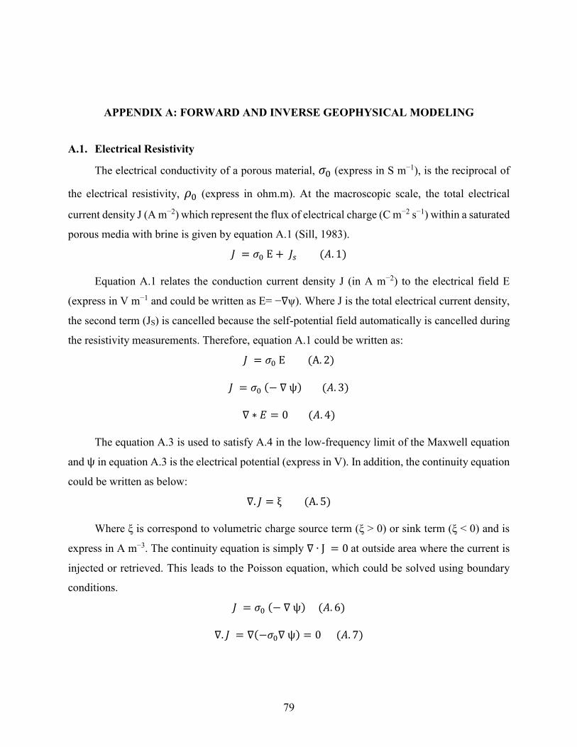
79
APPENDIX A: FORWARD AND INVERSE GEOPHYSICAL MODELING
A.1. Electrical Resistivity
The electrical conductivity of a porous material, 𝜎0 (express in S m−1), is the reciprocal of
the electrical resistivity, 𝜌0 (express in ohm.m). At the macroscopic scale, the total electrical
current density J (A m−2) which represent the flux of electrical charge (C m−2 s−1) within a saturated
porous media with brine is given by equation A.1 (Sill, 1983).
𝐽 = 𝜎0 E + 𝐽𝑠 (𝐴. 1)
Equation A.1 relates the conduction current density J (in A m−2) to the electrical field E
(express in V m−1 and could be written as E= −∇ψ). Where J is the total electrical current density,
the second term (JS) is cancelled because the self-potential field automatically is cancelled during
the resistivity measurements. Therefore, equation A.1 could be written as:
𝐽 = 𝜎0 E (A. 2)
𝐽 = 𝜎0 (− ∇ ψ) (𝐴. 3)
∇ ∗ 𝐸 = 0 (𝐴. 4)
The equation A.3 is used to satisfy A.4 in the low-frequency limit of the Maxwell equation
and ψ in equation A.3 is the electrical potential (express in V). In addition, the continuity equation
could be written as below:
∇. 𝐽 = ξ (A. 5)
Where ξ is correspond to volumetric charge source term (ξ > 0) or sink term (ξ < 0) and is
express in A m−3. The continuity equation is simply ∇ ∙ J = 0 at outside area where the current is
injected or retrieved. This leads to the Poisson equation, which could be solved using boundary
conditions.
𝐽 = 𝜎0 (− ∇ ψ) (𝐴. 6)
∇. 𝐽 = ∇(−𝜎0∇ ψ) = 0 (𝐴. 7)

80
Figure A.1. Measured concentrations in the large column effluent (orange triangles) and
calculated concentrations in forward modeling using COMSOL Multiphysics (black line) for the
first tracer test-Decay part. Concentrations of Na, SO42−, Al, Ca, Fe, and Mg quantified with
inductively coupled plasma–optical emission spectroscopy (ICP-OES), while alkalinity was
determined by titration. The red line is the concentration of Br within the column effluent measured
with bromide electrode.

81
APPENDIX B: MASS PACKED INSIDE COLUMNS
Table B.1. Masses of materials used in packing the small columns.
Column Sand (g) Coke (g) Sand (g)
DC - DIa 226.13 822.81 249.46
SC - DI 245.76 781.72 228.36
DC - OPSWb 215.51 804.12 233.51
SC - OSPW 225.04 791.12 239.84
DC - ARDc 221.13 765.35 255.54
SC - ARD 230.67 789.99 224
aDI: Deionized water
bOSPW: Oil sand process-affected water
cARD: Acid rock drainage
Table B.2. Masses of materials used in packing the large column.
Length (cm) Material Weight (kg)
8.5 (top) Sand 3.20
10 Coke 2.11
10 Coke 2.23
10 Coke 2.23
10 Coke 1.96
10 Coke 2.12
8.5 (base) Sand 3.00

82
APPENDIX C: CATION EXCHANGE CAPACITY
Methods from Holden et al. (2012) and Santamarina et al. (2002) were combined to measure
the cation exchange capacity (CEC) of the coke particles. Frist, 90 g of oven dried fresh dry and
slurry coke were soaked with 0.5 L Milli-Q water in a 1 L clean beaker and stirred for 20 min.
Since we expected a very low CEC value for fresh dry coke, it was titrated with 0.0001 N
methylene blue (MB), while the slurry coke was titrated with 0.001 N MB. In contrast with original
methods, 0.0001 N and 0.001 N MB were used in this experiment instead of 0.01 N MB (to prevent
the formation of dimers or other orientations of the methylene blue molecules which could over-
estimate the CEC value; also, the lower concentration results in a more sensitive end point). MB
was added in 1 mL increments and stirred for 1 min. A glass stir rod was used to place one drop
of the suspension on Whatman 42 ashless filter paper (spot test). At each step, 5 mL of suspension
was centrifuged, then 2 mL of the solution was pipetted into 3 mL cuvettes and the absorption was
measured using a DR2800 Spectrophotometer at a single wavelength of 664 nm (titration method).
Based on the MB standard curve, MB concentration in the solution was measured. The centrifuged
solution was returned into the beaker, the amount of absorbed MB was plotted against the added
MB, and the divergent point of the graph compared with line 45 is the point of complete cation
replacement, meaning all available sites are occupied with MB. MB was added until the final point
was reached (consistent halo), meaning all available sites on the surface are replaced with
methylene blue molecules. Adding MB was continued even after the halo point to see if the halo
was consistent. Because of non-linear methylene blue absorption, Absorbance should be lower
than 1, otherwise dilution should be performed. Finally, the CEC value is measured based on
amount of MB to reach the halo point and the divergent point (Spot and titration method).
Following Kaminsky (2014), 1 g of oven dried sample was soaked in 50 mL Milli-Q water
inside a clean 250 mL beaker (n = 8). One beaker was titrated with 0.0001 N MB (due to very low
CEC values and the small amount of coke particles that were used in this part of the experiment)
until it reached the end halo point (spot test). At this point, four beakers were titrated with smaller
amount of MB than the end point (in 1 mL increments), and three were titrated with a higher
amounts than the end point (in 1 mL increments). All beakers were stirred for 2 h and one drop
was placed on Whatman 42 ashless filter paper for each beaker to get the halo point (spot test).
The beakers were allowed to settle overnight. The next day, 10 mL from each beaker was
centrifuged and the MB concentration inside each beaker was measured using a DR2800
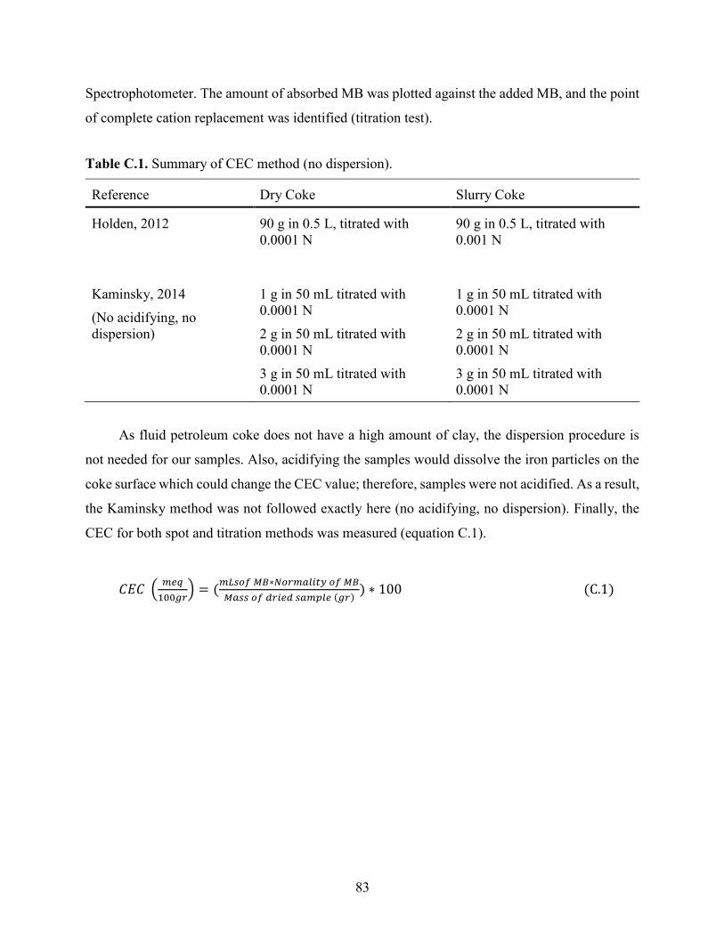
83
Spectrophotometer. The amount of absorbed MB was plotted against the added MB, and the point
of complete cation replacement was identified (titration test).
Table C.1. Summary of CEC method (no dispersion).
Reference Dry Coke Slurry Coke
Holden, 2012 90 g in 0.5 L, titrated with
0.0001 N
90 g in 0.5 L, titrated with
0.001 N
Kaminsky, 2014
(No acidifying, no
dispersion)
1 g in 50 mL titrated with
0.0001 N
2 g in 50 mL titrated with
0.0001 N
3 g in 50 mL titrated with
0.0001 N
1 g in 50 mL titrated with
0.0001 N
2 g in 50 mL titrated with
0.0001 N
3 g in 50 mL titrated with
0.0001 N
As fluid petroleum coke does not have a high amount of clay, the dispersion procedure is
not needed for our samples. Also, acidifying the samples would dissolve the iron particles on the
coke surface which could change the CEC value; therefore, samples were not acidified. As a result,
the Kaminsky method was not followed exactly here (no acidifying, no dispersion). Finally, the
CEC for both spot and titration methods was measured (equation C.1).
𝐶𝐸𝐶 (𝑚𝑒𝑞
100𝑔𝑟) = (
𝑚𝐿𝑠𝑜𝑓 𝑀𝐵∗𝑁𝑜𝑟𝑚𝑎𝑙𝑖𝑡𝑦 𝑜𝑓 𝑀𝐵
𝑀𝑎𝑠𝑠 𝑜𝑓 𝑑𝑟𝑖𝑒𝑑 𝑠𝑎𝑚𝑝𝑙𝑒 (𝑔𝑟)) ∗ 100 (C.1)

84
Table C.2. CEC values for fresh dry coke (no dispersion).
Titration method Spot test
1 g, 50 mL MQa, 0.0001 N MB 0.02 meq/100 g 0.04 meq/100 g
2 g, 50 mL MQ, 0.0001 N MB 0.03 meq/100 g 0.03 meq/100 g
3 g, 50 mL MQ, 0.0001 N MB 0.02 meq/100 g 0.017 meq/100 g
90 g, 500 mL MQ, 0.0001 N MB 0.049 meq/100 g 0.053 meq/100 g
aMQ: Milli-Q water
Table C.3. CEC for fresh slurry coke (no dispersion).
Titration method Spot test
1 g, 50 mL MQa, 0.0001 N MB 0.19 meq/100 g 0.2 meq/100 g
2 g, 50 mL MQ, 0.0001 N MB 0.205 meq/100 g 0.21 meq/100 g
3 g, 50 mL MQ, 0.0001 N MB 0.20 meq/100 g 0.21 meq/100 g
90 g, 500 mL MQ, 0.001 N MB 0.20 meq/100 g 0.211 meq/100 g
aMQ: Milli-Q water
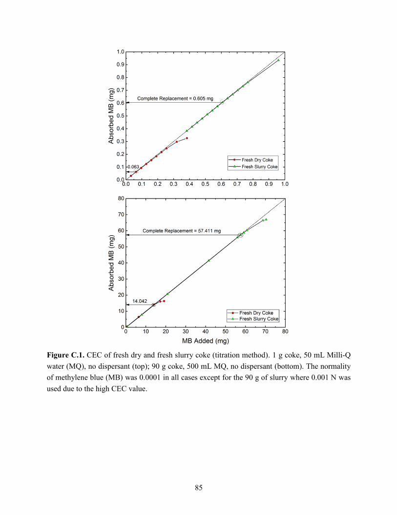
85
Figure C.1. CEC of fresh dry and fresh slurry coke (titration method). 1 g coke, 50 mL Milli-Q
water (MQ), no dispersant (top); 90 g coke, 500 mL MQ, no dispersant (bottom). The normality
of methylene blue (MB) was 0.0001 in all cases except for the 90 g of slurry where 0.001 N was
used due to the high CEC value.

86
APPENDIX D: VANADIUM (V) REACTIONS AND FORMATION CONSTANT
Table D.1. Aqueous V(V) reactions and equilibrium constants considered for thermodynamic
modeling.
Reaction log K Reference
VO2+ + 2H2O ↔ VO4
3– + 4H+ –29.38 a, b*
VO2+ + 2H2O ↔ HVO4
2– + 3H+ –15.89 a, b *
VO2+ + 2H2O ↔ H2VO4
– + 2H+ –7.14 a, b *
2VO2+ + 3H2O ↔ V2O7
4– + 6H+ –32.88 a, b *
2VO2+ + 3H2O ↔ HV2O7
3– + 5H+ –21.58 a, b *
2VO2+ + 3H2O ↔ H2V2O7
2– + 4H+ –11.98 a, b *
3VO2+ + 4H2O ↔ HV3O10
4– + 7H+ –26.71 c, d*
4VO2+ + 5H2O ↔ V4O13
6– + 10H+ –43.01 a, b *
4VO2+ + 5H2O ↔ HV4O13
5– + 9H+ –32.23 a, b *
4VO2+ + 4H2O ↔ V4O12
4– + 8H+ –20.96 a, b *
5VO2+ + 5H2O ↔ V5O15
5– + 10H+ –27.43 a, b *
6VO2+ + 6H2O ↔ V6O18
6– + 12H+ –34.55 a, b *
10VO2+ + 8H2O ↔ V10O28
6– + 16H+ –24.76 a, b *
10VO2+ + 8H2O ↔ HV10O28
5– + 15H+ –17.4 a, b *
10VO2+ + 8H2O ↔ H2V10O28
4– + 14H+ –13.2 a, b *
10VO2+ + 8H2O ↔ H3V10O28
3– + 13H+ –8.52 a, b *
a(Cruywagen et al., 1996)
b(Cruywagen, 1999)
c(McCann et al., 2013)
d(McCann et al., 2015)
e(Smith et al., 2004)
f(Larson, 1995)
g(Elvingson et al., 1996)
*Used in this stud

87
APPENDIX E: PH POINT OF ZERO CHARGE
Table E.1. Summary of pH of point of zero charge (pHPCZ) for fresh dry coke.
DC1a DC2 DC3
Initial
pH
Final
pH ΔpH
Initial
pH
Final
pH ΔpH
Initial
pH
Final
pH ΔpH
2.05 2.42 0.37 2.04 2.5 0.46 2.26 2.47 0.21
2.97 3.23 0.26 3.08 3.36 0.28 3.23 3.3 0.07
3.95 4.26 0.31 4.02 4.37 0.35 4.04 4.64 0.6
4.95 5.31 0.36 5.22 5.56 0.34 4.87 5.63 0.76
5.79 6.14 0.35 6.14 6.38 0.24 5.83 6.13 0.3
7.25 6.77 −0.48 6.73 6.77 0.04 6.88 6.84 −0.04
7.78 6.96 −0.82 8.26 7.04 −1.22 7.7 7.18 −0.52
9.3 8.01 −1.29 9.1 7.21 −1.89 8.82 7.58 −1.24
10.04 9.07 −0.97 9.97 8.34 −1.63 10.3 10.08 −0.22
pHPZC 6.4 6.78 6.76
aDC: Dry coke

88
Table E.2. Summary of pH of point of zero charge (pHPCZ) for fresh slurry coke.
SC1a SC2 SC3
Initial
pH
Final
pH ΔpH
Initial
pH Final pH ΔpH
Initial
pH
Final
pH ΔpH
2.04 2.53 0.49 2.04 2.51 0.47 2.28 2.35 0.07
3.05 3.42 0.37 3.13 3.54 0.41 3.24 3.6 0.36
3.91 5.1 1.19 4.04 5.74 1.7 4.03 5.84 1.81
4.84 6.85 2.01 5.04 6.62 1.58 4.75 6.61 1.86
6.24 6.74 0.5 6.26 7.16 0.9 5.8 6.77 0.97
7.23 7.31 0.08 7.05 6.92 −0.13 6.88 7.26 0.38
7.88 7.38 −0.5 8.11 7.51 −0.6 8.01 7.35 −0.66
9.14 7.79 −1.35 9.04 7.64 −1.4 8.92 7.84 −1.08
9.73 8.55 −1.18 9.77 8.3 −1.47 10.3 9.98 −0.32
pHPZC 7.32 6.95 7.29
aSC: Slurry coke
Figure E.1. The pH point of zero charge (pHPCZ) for fresh coke particles (dry and slurry coke).
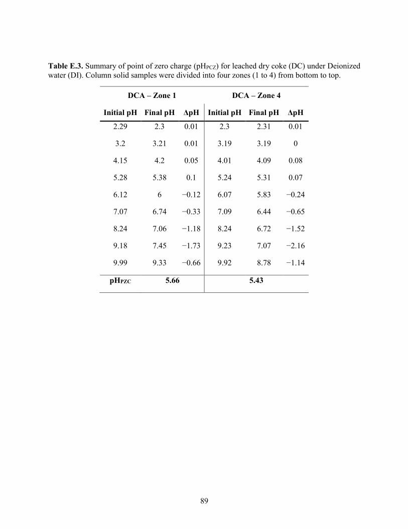
89
Table E.3. Summary of point of zero charge (pHPCZ) for leached dry coke (DC) under Deionized
water (DI). Column solid samples were divided into four zones (1 to 4) from bottom to top.
DCA – Zone 1 DCA – Zone 4
Initial pH Final pH ΔpH Initial pH Final pH ΔpH
2.29 2.3 0.01 2.3 2.31 0.01
3.2 3.21 0.01 3.19 3.19 0
4.15 4.2 0.05 4.01 4.09 0.08
5.28 5.38 0.1 5.24 5.31 0.07
6.12 6 −0.12 6.07 5.83 −0.24
7.07 6.74 −0.33 7.09 6.44 −0.65
8.24 7.06 −1.18 8.24 6.72 −1.52
9.18 7.45 −1.73 9.23 7.07 −2.16
9.99 9.33 −0.66 9.92 8.78 −1.14
pHPZC 5.66 5.43

90
Table E.4. Summary of pH of point of zero charge (pHPCZ) for leached slurry coke (SC) under
deionized water (DI). Column solid samples were divided into four zones (1 to 4) from bottom to
top.
SCD – Zone 1 SCD – Zone 4
Initia pH Final pH ΔpH Initia pH Final pH ΔpH
2.29 2.32 0.03 2.29 2.48 0.19
3.2 3.59 0.39 3.19 3.3 0.11
4.04 4.39 0.35 3.98 4.43 0.45
5.21 5.42 0.21 5.25 5.79 0.54
6.08 5.94 −0.14 6.01 5.76 −0.25
7.01 6.5 −0.51 6.92 6.25 −0.67
8.23 6.72 −1.51 8.11 6.68 −1.43
9.24 7.8 −1.44 9.19 6.91 −2.28
9.91 8.22 −1.69 9.93 7.66 −2.27
pHPZC 5.73 5.77

91
Table E.5. Summary of pH of point of zero charge (pHPCZ) for leached dry coke (DC) under oil
sand process-affected water (OSPW). Column solid samples were divided into four zones (1 to 4)
from bottom to top.
DCC – Zone 1 DCC – Zone 1
Initial pH Final pH ΔpH Initial pH Final pH ΔpH
2.22 2.23 0.01 2.3 2.48 0.19
3.06 3.1 0.04 3.17 3.3 0.11
3.84 3.99 0.15 3.99 4.43 0.45
5.12 5.54 0.42 4.71 5.79 0.54
6 6.18 0.18 6.18 5.76 −0.25
6.95 6.78 −0.17 7.08 6.25 −0.67
8.23 7.09 −1.14 8.11 6.68 −1.43
8.88 7.51 −1.37 8.79 6.91 −2.28
9.94 9.45 −0.49 9.84 7.66 −2.27
pHPZC 6.49 6.45

92
Table E.6. Summary of pH of point of zero charge (pHPCZ) for leached dry coke (DC) under oil
sand process-affected water (OSPW). Column solid samples were divided into four zones (1 to 4)
from bottom to top.
DCC – Zone4 DCC – Zone4 DCC – Zone4
Initial
pH
Final
pH ΔpH
Initial
pH
Final
pH ΔpH
Initial
pH
Final
pH ΔpH
2.21 2.21 0 2.29 2.35 0.06 2.28 2.29 0.01
3.06 3.09 0.03 3.24 3.38 0.14 3.24 3.41 0.17
3.82 4.6 0.78 4.14 4.46 0.32 4.03 4.34 0.31
5.11 5.32 0.21 4.78 5.4 0.62 4.89 5.58 0.69
5.79 5.91 0.12 5.85 6.21 0.36 5.8 6.11 0.31
6.76 6.26 −0.5 6.89 6.6 −0.29 6.88 6.61 −0.27
8.25 6.63 −1.62 8.06 7.29 −0.77 7.8 7.15 −0.65
8.83 6.89 −1.94 8.96 7.75 −1.21 9.07 7.76 −1.31
9.94 8.68 −1.26 10.28 10.08 −0.2 10.3 10.08 −0.22
pHPZC 5.98 6.43 6.38

93
Table E.7. Summary of pH of point of zero charge (pHPCZ) for leached slurry coke (SC) under oil
sand process-affected water (OSPW). Column solid samples were divided into four zones (1 to 4)
from bottom to top.
SCF – Zone 1 SCF – Zone 1 SCF – Zone
4
Initial
pH
Final
pH ΔpH
Initial
pH
Final
pH ΔpH
Initial
pH
Final pH ΔpH
2.2 2.21 0.01 2.3 2.35 0.05 2.2 2.22 0.02
3.06 3.2 0.14 3.16 3.59 0.43 3.05 3.24 0.19
3.82 4.45 0.63 4.02 5.02 1 3.82 4.53 0.71
5.11 6.44 1.33 5.2 6.38 1.18 5.16 5.81 0.65
5.77 6.37 0.6 6.26 6.61 0.35 5.77 6.04 0.27
6.71 6.94 0.23 6.95 6.9 −0.05 6.9 6.41 −0.49
8.26 7.22 −1.04 7.7 7.08 −0.62 8.26 6.59 −1.67
8.83 7.31 −1.52 8.73 7.27 −1.46 8.86 6.87 −1.99
9.91 9.21 −0.7 9.87 7.58 −2.29 9.9 7.93 −1.97
pHPZC 6.99 6.86 6.17

94
Table E.8. Summary of pH of point of zero charge (pHPCZ) for leached dry coke (DC) under acid
rock drainage (ARD). Column solid samples were divided into four zones (1 to 4) from bottom to
top.
DCB – Zone 1
Initial pH Final pH ΔpH
2.3 2.44 0.14
3.2 3.33 0.13
4.09 4.1 0.01
4.92 4.48 −0.44
6.14 5.06 −1.08
7.17 5.77 −1.4
7.71 6.32 −1.39
8.81 6.43 −2.38
9.85 7.49 −2.36
pHPZC 4.11

95
Table E.9. Summary of pH of point of zero charge (pHPCZ) for leached dry coke (DC) under acid
rock drainage (ARD). Column solid samples were divided into four zones (1 to 4) from bottom to
top.
DCB – Zone4 DCB – Zone4 DCB – Zone4
Initial
pH
Final
pH ΔpH
Initial
pH
Final
pH ΔpH
Initial
pH
Final
pH ΔpH
2.3 2.31 0.01 2.24 2.32 0.08 2.28 2.32 0.04
3.17 3.47 0.3 3.2 3.35 0.15 3.23 3.13 −0.1
4.06 4.48 0.42 4.27 4.46 0.19 4.02 4.22 0.2
4.71 4.98 0.27 4.73 4.74 0.01 4.86 4.86 0
6.19 5.57 −0.62 5.88 5.49 −0.39 5.97 5.68 −0.29
7.08 6.39 −0.69 7.3 6.86 −0.44 6.89 6.62 −0.27
7.74 6.79 −0.95 7.72 6.94 −0.78 7.97 6.94 −1.03
8.78 6.93 −1.85 9.18 7.99 −1.19 8.98 7.33 −1.65
9.89 7.76 −2.13 9.89 8.8 −1.09 10.28 9.86 −0.42
pHPZC 5.16 4.76 4.86
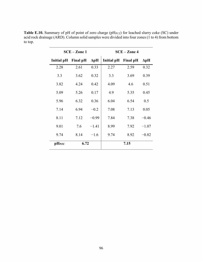
96
Table E.10. Summary of pH of point of zero charge (pHPCZ) for leached slurry coke (SC) under
acid rock drainage (ARD). Column solid samples were divided into four zones (1 to 4) from bottom
to top.
SCE – Zone 1 SCE – Zone 4
Initial pH Final pH ΔpH Initial pH Final pH ΔpH
2.28 2.61 0.33 2.27 2.59 0.32
3.3 3.62 0.32 3.3 3.69 0.39
3.82 4.24 0.42 4.09 4.6 0.51
5.09 5.26 0.17 4.9 5.35 0.45
5.96 6.32 0.36 6.04 6.54 0.5
7.14 6.94 −0.2 7.08 7.13 0.05
8.11 7.12 −0.99 7.84 7.38 −0.46
9.01 7.6 −1.41 8.99 7.92 −1.07
9.74 8.14 −1.6 9.74 8.92 −0.82
pHPZC 6.72 7.15

97
Table E.11. Summary of pH of point of zero charge (pHPCZ) for big column (sequential input
solution, i.e., deionized water, oil sand process-affected water, and acid rock drainage). Column
solid samples were divided into five zones (1 to 5) from bottom to top.
LC – Zone1 LC – Zone 5
Initial pH Final pH ΔpH Initial pH Final pH ΔpH
2.26 2.55 0.29 2.26 2.53 0.27
3.3 3.74 0.44 3.28 3.6 0.32
3.99 4.69 0.7 4.02 4.66 0.64
5.26 5.54 0.28 5.3 5.92 0.62
6.03 6.68 0.65 6.1 6.79 0.69
7.04 7.31 0.27 7.05 7.35 0.3
7.74 7.7 −0.04 7.74 7.76 0.02
8.96 8.77 −0.19 8.99 8.85 −0.14
9.75 9.55 −0.2 9.75 9.53 −0.22
pHPZC 7.65 7.9
aLC: Large column

98
Table E.12. Summary of pH of point of zero charge (pHPCZ) for big column (sequential input
solution, i.e., deionized water, oil sand process-affected water, and acid rock drainage). Column
solid samples were divided into five zones (1 to 5) from bottom to top.
LCa – Zone3 LC – Zone3 LC – Zone3
Initial
pH
Final
pH ΔpH
Initial
pH
Final
pH ΔpH
Initial
pH
Final
pH ΔpH
2.26 2.56 0.3 2.3 2.35 0.05 2.24 2.3 0.06
3.28 3.64 0.36 3.27 3.38 0.11 3.25 3.39 0.14
4.03 4.77 0.74 4.09 4.36 0.27 4.04 4.33 0.29
5.28 5.89 0.61 5.04 5.12 0.08 4.76 4.95 0.19
6.06 6.75 0.69 6 6.08 0.08 6.02 6.02 0
7.06 7.36 0.3 6.85 6.69 −0.16 6.92 6.62 −0.3
7.74 7.7 −0.04 8.21 7.22 −0.99 8.08 7.11 −0.97
9.01 8.79 −0.22 8.93 7.66 −1.27 8.7 7.49 −1.21
9.78 9.6 −0.18 10.23 10.01 −0.22 10.26 10.01 −0.25
pHPZC 7.66 6.28 6.02
aLC: Large column

99
Figure E.2. The pH point of zero charge (pHPZC) results for leached coke particle. Samples were
obtained from zones 1 and 4 of the columns (Zone 1 is the area close to inflow, and zone 4 is close
to the outflow).

100
Table E.13. The pH point of zero charge (pHPZC) results for the small columns (leached samples).
Sample code Zone 1 Zone 4
DC - DIa 5.66 5.43
SC - DI 5.73 5.77
DC - OSPWb 6.46 6.26 ±0.2
SC - OSPW 6.93 6.17
DC - ARDc 4.11 4.93 ± 0.17
SC - ARD 6.72 7.15 aDI: Deionized water
bOSPW: oil sand processing affected water
cARD
DC: Dry coke
SC: Slurry coke
Table E.14. The pH point of zero charge (pHPZC) results for the large column in different zones.
Column solid samples were divided into five zones (1 to 5) from bottom to top.
Zone 1 Zone 3 Zone 5
Large Column 7.65 6.65 ± 0.72 7.9

101
APPENDIX F: BULK ELEMENTAL ANALYSES
Table F.1. Bulk elemental analyses for the columns (LC: large column, SC: small columns). All
values are in mg kg−1.
Sample ID C
LECO
S
LCEO
Si
Al
Fe
Ca
Zr V Ti K
LC-10 788000 79800 14023 7463 5176 1930 2690 1360 1379 1079
LC-20 819000 79800 13556 7251 5036 1858 5380 1350 1379 996
LC-30 782000 79800 12620 7039 5386 1930 2030 1410 1438 1079
LC-40 778000 79900 13089 7039 5595 1930 2450 1430 1438 1162
LC-50 782400 80100 12154 6881 5316 1930 1580 1420 1379 1079
DC-A1 798000 78300 11686 6828 4966 1787 2590 1300 1319 996
DC-A3 778000 84700 14958 7198 5386 2430 1360 1350 1319 1079
SC-D1 793500 79800 13089 7251 5106 2073 3800 1380 1438 1079
SC-D2 801000 79200 11686 6933 4896 2001 1870 1350 1379 996
DC-B2 822000 80200 11686 6881 4966 1787 1380 1320 1319 996
DC-B3 791000 80600 13089 6986 5246 2073 1620 1420 1498 1079
SC-E1 784000 80200 13556 7198 5456 2359 2720 1460 1558 1079
SC-E2 812000 79900 12154 6881 5106 2073 1570 1400 1438 1079
DC-C1 780000 79000 11686 6881 4896 1858 1300 1320 1319 1079
DC-C2 785000 79400 11686 6828 5456 1787 1840 1320 1319 996
SC-F1 793000 80300 12621 6881 5176 2073 2570 1400 1438 1079
SC-F3 786000 80500 13556 7039 5316 2073 4300 1400 1498 1079
LC : Large column
DC: Dry coke
SC : Slurry coke

102
Continue Table F.1.
Sample ID Mg Na Ni P Sr Ba Mo Mn Ce
LC-10 784.0 445.1 513.0 218.2 76.0 85.0 72.5 77.4 55.0
LC-20 723.7 445.1 552.0 261.9 78.0 76.0 73.2 77.4 43.0
LC-30 784.0 519.3 573.0 261.9 78.0 90.0 77.3 77.4 34.0
LC-40 784.0 445.1 549.0 305.5 82.0 75.0 78.0 77.4 35.0
LC-50 784.0 445.1 528.0 261.9 83.0 73.0 76.6 77.4 33.0
DC-A1 784.0 445.1 516.0 261.9 79.0 76.0 75.5 77.4 34.0
DC-A3 784.0 519.3 540.0 305.5 79.0 80.0 72.8 77.4 37.0
SC-D1 844.3 667.7 537.0 261.9 83.0 76.0 77.0 77.4 41.0
SC-D2 784.0 667.7 519.0 261.9 77.0 78.0 71.9 77.4 53.0
DC-B2 723.7 445.1 523.0 261.9 79.0 90.0 70.9 77.4 31.0
DC-B3 844.3 667.7 540.0 218.2 80.0 85.0 73.7 77.4 85.0
SC-E1 844.3 741.9 573.0 261.9 84.0 90.0 85.0 77.4 44.0
SC-E2 844.3 667.7 528.0 261.9 85.0 86.0 75.4 77.4 39.0
DC-C1 723.7 445.1 534.0 261.9 80.0 77.0 73.0 77.4 35.0
DC-C2 784.0 445.1 537.0 218.2 78.0 75.0 74.3 77.4 77.0
SC-F1 784.0 667.7 543.0 261.9 80.0 82.0 74.4 77.4 38.0
SC-F3 844.3 741.9 564.0 261.9 80.0 87.0 77.2 77.4 47.0
LC : Large column
DC: Dry coke
SC : Slurry coke

103
Continue Table F.1.
Sample ID Cr Zn Y Nd La Cu Th Be Pb Co
LC-10 43.0 31.0 15.2 13.7 17.0 10.2 7.9 7.1 8.4 5.2
LC-20 40.0 34.0 19.6 14.2 17.0 13.0 6.8 8.3 6.0 6.0
LC-30 50.0 41.0 15 13.6 16.0 13.8 5.7 8.6 6.4 6.6
LC-40 55.0 36.0 16 14.1 16.0 10.7 6.2 8.5 6.7 6.6
LC-50 55.0 30.0 13.5 14.5 16.0 10.3 5.8 8.1 5.8 6.5
DC-A1 41.0 40.0 14.7 13.4 15.0 33.0 5.5 8.3 4.4 5.1
DC-A3 58.0 38.0 14.1 13.8 16.0 12.6 7.0 7.6 4.5 6.1
SC-D1 46.0 39.0 17.2 14.5 17.0 15.9 7.0 7.7 7.3 5.5
SC-D2 43.0 34.0 14.3 15.1 15.0 12.9 6.8 7.7 4.2 5.6
DC-B2 43.0 33.0 12.8 12.4 14.0 16.6 5.3 8.2 6.0 5.9
DC-B3 42.0 45.0 15 37.8 36.0 10.1 89.4 7.8 10.3 6.6
SC-E1 38.0 64.0 16.6 15.0 19.0 12.5 8.7 7.3 5.4 5.5
SC-E2 44.0 37.0 13.7 16.0 19.0 14.0 5.8 7.8 6.0 5.4
DC-C1 39.0 33.0 12.9 14.2 17.0 16.6 5.6 7.7 11.4 5.4
DC-C2 42.0 56.0 15.9 16.7 22.0 14.3 5.2 7.2 5.6 6.2
SC-F1 64.0 33.0 16.1 15.2 18.0 102.0 7.5 8.0 6.8 5.4
SC-F3 55.0 57.0 20.3 17.4 21.0 43.8 13.6 8.6 7.0 5.0
LC : Large column
DC: Dry coke
SC : Slurry coke
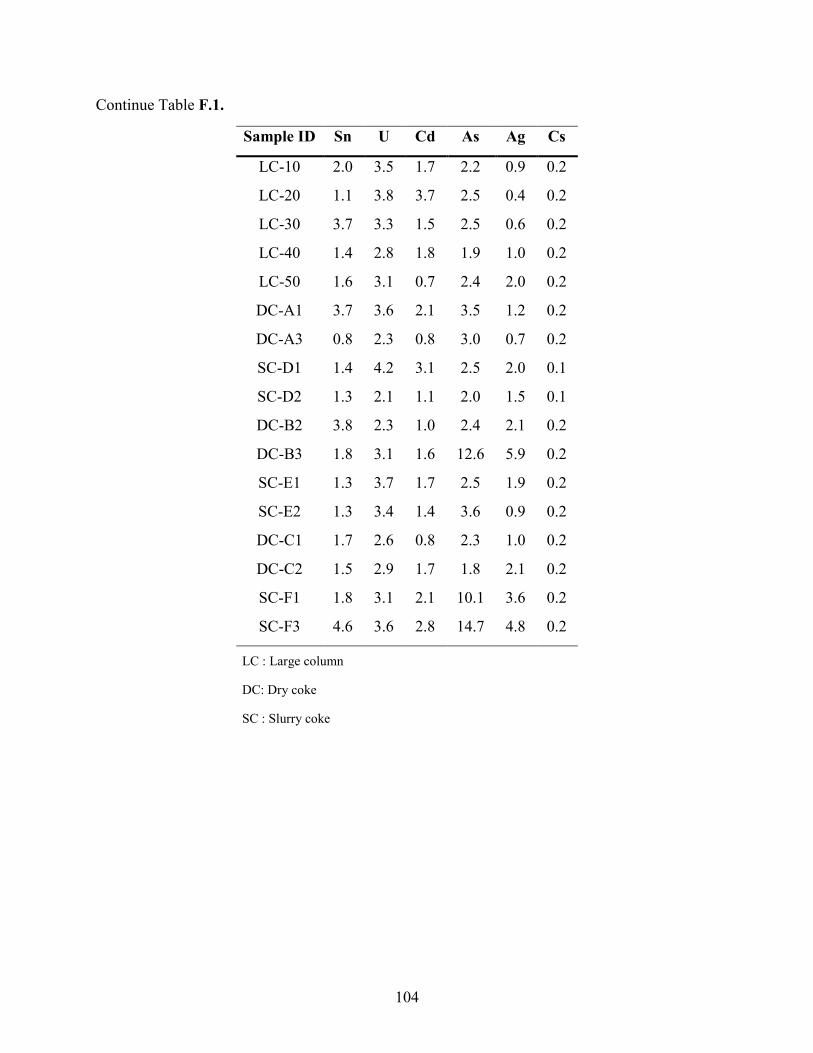
104
Continue Table F.1.
Sample ID Sn U Cd As Ag Cs
LC-10 2.0 3.5 1.7 2.2 0.9 0.2
LC-20 1.1 3.8 3.7 2.5 0.4 0.2
LC-30 3.7 3.3 1.5 2.5 0.6 0.2
LC-40 1.4 2.8 1.8 1.9 1.0 0.2
LC-50 1.6 3.1 0.7 2.4 2.0 0.2
DC-A1 3.7 3.6 2.1 3.5 1.2 0.2
DC-A3 0.8 2.3 0.8 3.0 0.7 0.2
SC-D1 1.4 4.2 3.1 2.5 2.0 0.1
SC-D2 1.3 2.1 1.1 2.0 1.5 0.1
DC-B2 3.8 2.3 1.0 2.4 2.1 0.2
DC-B3 1.8 3.1 1.6 12.6 5.9 0.2
SC-E1 1.3 3.7 1.7 2.5 1.9 0.2
SC-E2 1.3 3.4 1.4 3.6 0.9 0.2
DC-C1 1.7 2.6 0.8 2.3 1.0 0.2
DC-C2 1.5 2.9 1.7 1.8 2.1 0.2
SC-F1 1.8 3.1 2.1 10.1 3.6 0.2
SC-F3 4.6 3.6 2.8 14.7 4.8 0.2
LC : Large column
DC: Dry coke
SC : Slurry coke
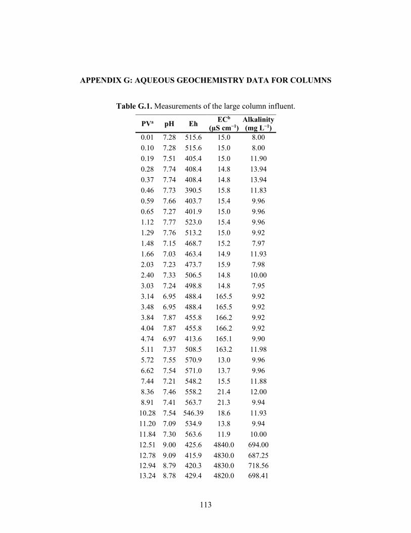
113
APPENDIX G: AQUEOUS GEOCHEMISTRY DATA FOR COLUMNS
Table G.1. Measurements of the large column influent.
PVa pH Eh ECb
(µS cm−1)
Alkalinity
(mg L−1)
0.01 7.28 515.6 15.0 8.00
0.10 7.28 515.6 15.0 8.00
0.19 7.51 405.4 15.0 11.90
0.28 7.74 408.4 14.8 13.94
0.37 7.74 408.4 14.8 13.94
0.46 7.73 390.5 15.8 11.83
0.59 7.66 403.7 15.4 9.96
0.65 7.27 401.9 15.0 9.96
1.12 7.77 523.0 15.4 9.96
1.29 7.76 513.2 15.0 9.92
1.48 7.15 468.7 15.2 7.97
1.66 7.03 463.4 14.9 11.93
2.03 7.23 473.7 15.9 7.98
2.40 7.33 506.5 14.8 10.00
3.03 7.24 498.8 14.8 7.95
3.14 6.95 488.4 165.5 9.92
3.48 6.95 488.4 165.5 9.92
3.84 7.87 455.8 166.2 9.92
4.04 7.87 455.8 166.2 9.92
4.74 6.97 413.6 165.1 9.90
5.11 7.37 508.5 163.2 11.98
5.72 7.55 570.9 13.0 9.96
6.62 7.54 571.0 13.7 9.96
7.44 7.21 548.2 15.5 11.88
8.36 7.46 558.2 21.4 12.00
8.91 7.41 563.7 21.3 9.94
10.28 7.54 546.39 18.6 11.93
11.20 7.09 534.9 13.8 9.94
11.84 7.30 563.6 11.9 10.00
12.51 9.00 425.6 4840.0 694.00
12.78 9.09 415.9 4830.0 687.25
12.94 8.79 420.3 4830.0 718.56
13.24 8.78 429.4 4820.0 698.41

114
PVa pH Eh ECb
(µS cm−1)
Alkalinity
(mg L−1)
13.31 8.85 379.65 4810.0 710.58
13.41 8.83 392.41 4800.0 715.71
13.69 8.70 440.40 4760.0 706.11
13.96 8.62 388.33 4770.0 688.98
14.50 8.69 421.99 4700.0 704.59
15.06 8.47 424.19 4700.0 718.00
15.87 8.47 424.19 4700.0 718.00
17.40 8.54 423.34 4840.0 714.29
18.23 8.64 426.40 4810.0 731.06
18.56 8.57 410.20 4810.0 718.56
19.11 8.70 451.88 4760.0 707.17
19.77 8.70 451.88 4760.0 717.13
20.13 8.69 424.90 4880.0 716.00
20.23 8.75 426.00 4830.0 716.00
20.48 8.67 407.87 4830.0 693.00
20.88 8.40 385.20 4880.0 714.30
21.87 8.40 385.20 4880.0 714.30
22.23 8.39 366.49 4830.0 715.71
22.88 8.39 366.49 4830.0 715.71
23.41 8.68 396.51 4680.0 714.29
23.94 8.81 461.90 4610.0 685.48
24.98 8.89 286.31 5170.0 938.12
25.79 8.90 286.31 5170.0 938.12
26.22 8.88 286.31 5170.0 938.12
26.39 8.89 286.31 5170.0 938.12
26.67 8.92 290.11 5080.0 924.15
26.76 8.99 332.70 4970.0 920.32
27.03 8.89 370.71 4900.0 910.89
27.65 8.91 394.15 4930.0 909.82
28.31 8.60 359.13 4900.0 914.51
28.96 8.82 447.63 4880.0 885.83
29.59 8.74 426.73 4810.0 878.73
30.20 7.23 521.37 165.5 7.95
30.84 7.23 521.37 165.5 7.95
31.46 7.23 521.37 165.5 7.95
31.95 7.75 491.19 168.5 11.95
32.10 7.23 522.09 13.7 7.95
32.47 7.15 520.80 12.1 8.00
32.76 7.23 522.09 13.7 7.95
33.38 7.23 522.09 13.7 7.95
33.61 7.09 524.80 11.2 8.22

115
PVa pH Eh ECb
(µS cm−1)
Alkalinity
(mg L−1)
33.74 7.06 505.19 11.6 11.93
34.02 7.40 511.2 11.4 11.98
34.56 7.35 488.4 11.5 9.92
35.26 1.98 826.6 8770 –
35.89 2.10 828.6 8540 –
35.93 2.10 828.6 8540 –
36.02 2.10 828.6 8540 –
36.11 2.36 827.1 8700 –
36.20 2.35 826.8 8610 –
36.31 2.34 831.0 8670 –
36.39 2.20 829.8 8510 –
36.45 2.20 829.8 8510 –
36.54 2.42 827.7 8530 –
36.98 1.93 818.1 8940 –
37.19 1.97 830.9 9350 –
37.77 1.97 830.6 9350 –
38.03 2.07 825 8950 –
38.57 2.06 815.6 9060 –
38.85 2.04 826.6 8950 –
39.04 2.01 826.0 8940 –
39.10 2.01 826.0 8940 –
39.24 2.06 832.1 8790 –
39.30 2.06 832.6 8930 –
39.40 2.06 832.6 8930 –
39.57 2.06 830.4 9010 –
40.05 2.03 829.8 9030 –
40.39 2.03 829.8 9030 –
40.96 1.98 790.2 9880 –
41.67 1.92 788.6 9720 –
42.24 1.91 787.9 9700 –
42.47 1.98 812.5 9700 –
42.73 2.01 722.7 9580 –
aPV: Pore volume bEC: Electrical conductivity

116
Table G.2. Major cations concentrations in the large column influent quantified with inductively
coupled plasma–optical emission spectroscopy (ICP-OES).
PVa Ca Fe K Mg Na S
mg L−1 mg L−1 mg L−1 mg L−1 mg L−1 mg L−1
0.10 0.03 ud* 0.07 ud 3.27 0.11
0.19 ud ud 0.02 0.01 3.26 0.15
0.59 0.05 ud 0.02 0.02 3.24 0.19
0.65 0.05 ud 0.02 ud 3.22 0.11
1.29 0.04 ud 0.01 ud 3.18 0.12
2.40 0.05 ud 0.02 ud 3.20 0.11
3.03 0.09 ud 0.02 0.01 3.16 0.10
3.84 0.17 ud 0.04 0.01 29.64 0.11
5.11 0.12 ud 0.04 0.01 29.24 0.09
7.44 0.04 ud 0.02 ud 3.33 0.12
11.84 0.06 0.00 0.02 ud 2.59 0.20
12.51 2.57 ud 22.89 19.09 1100 75.5
12.78 2.30 ud 22.38 20.20 1130 84.2
12.94 8.05 ud 22.13 20.32 1130 83.6
13.24 5.86 ud 23.30 19.69 1140 77.4
13.31 5.85 ud 22.43 18.84 1120 73.4
13.41 5.60 ud 22.38 18.62 1150 73.1
13.69 4.51 ud 22.96 19.23 1150 75.6
13.96 6.10 ud 22.85 18.98 1120 74.0
19.77 3.46 ud 20.25 18.48 1050 71.8
23.94 3.70 ud 21.14 18.63 1110 74.03
26.22 5.72 ud 12.13 6.33 1140 191.3
27.65 6.10 ud 12.80 6.73 1170 204.0
29.59 6.06 ud 12.45 6.55 1155 197.0
36.11 394.0 2907 2.19 203.52 208 3680
37.19 400.8 2947 0.48 206.51 214 3820
38.03 422.2 2705 4.76 189.20 195 3349
39.24 395.9 2901 0.10 208.00 216 3687
39.57 386.3 2841 0.10 210.97 220 3649
40.39 427.6 2744 ud 195.80 196 3609
41.67 424.8 2796 ud 200.60 205 3758
42.24 412.3 2533 ud 199.01 202 3718 aPV: Pore volume *ud: concentrations below method detection limit

117
Table G.3. Trace element concentrations in the large column influent quantified by inductively
coupled plasma–optical mass spectroscopy (ICP-MS).
PVa Al Ba Ca Fe K Mg Mo
µg L−1 µg L−1 µg L−1 µg L−1 µg L−1 µg L−1 µg L−1
0.008 ud* ud ud ud ud ud ud
0.098
0.189 ud ud ud ud ud 34.86 ud
0.280
0.370
0.461
0.586 ud ud ud ud ud 20.04 ud
0.654
1.119
1.293 ud ud ud ud ud 15.58 ud
1.478
1.660
2.032
2.399
3.028
3.141
3.478
3.841 ud ud ud ud ud ud 0.87
4.037
4.741
5.111
5.722
6.616
7.444 ud ud ud ud ud ud ud
8.360
8.914
10.280
11.205
11.836 ud ud ud ud ud 13.75 1.45
12.509 ud ud 2405.62 ud 19439.84 19579.28 ud
12.781
12.944
13.235 ud ud 5723.39 ud 19974.97 20103.20 1.43
13.309 ud ud 5537.93 ud 20550.58 20187.39 5.30
13.405 ud ud 5327.62 ud 20222.52 20709.48 6.20
13.688 ud ud 4214.13 ud 20374.04 20457.02 9.09
13.957 ud ud 5970.17 ud 20491.69 20674.02 4.67
14.498
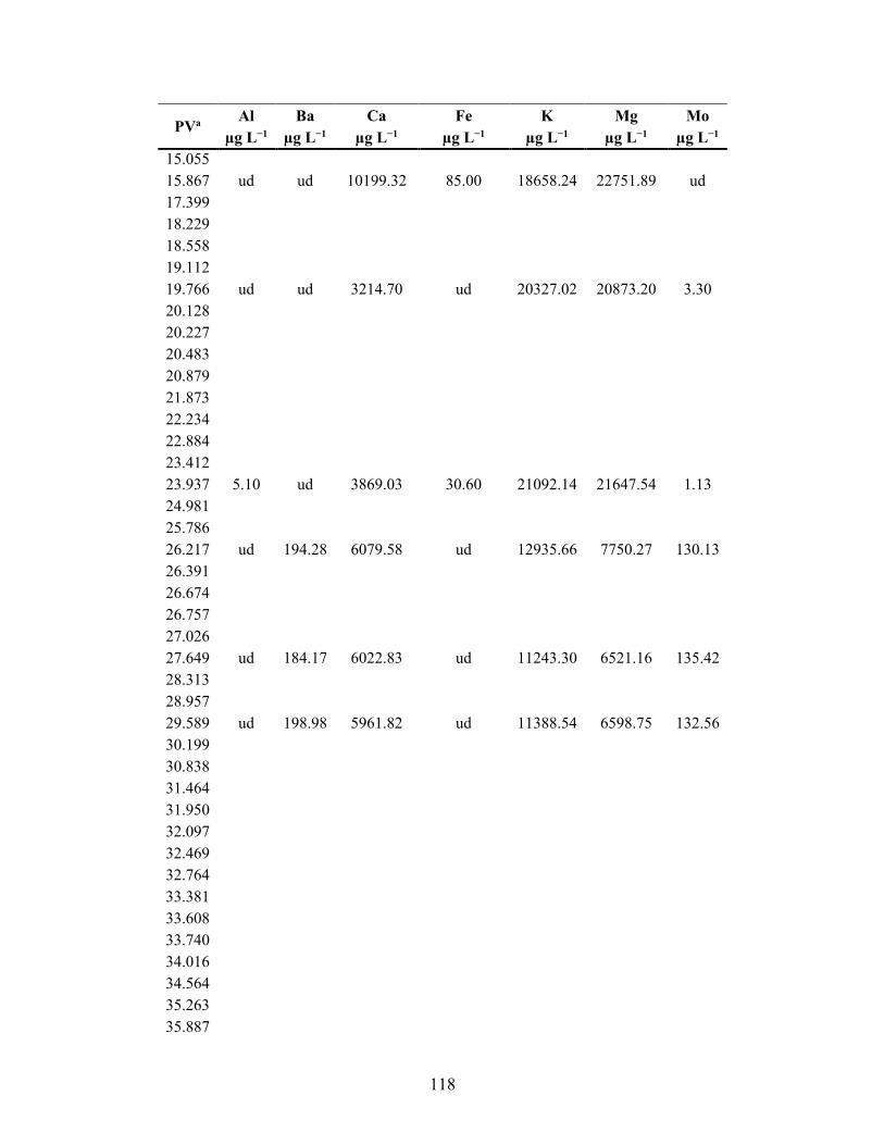
118
PVa Al Ba Ca Fe K Mg Mo
µg L−1 µg L−1 µg L−1 µg L−1 µg L−1 µg L−1 µg L−1
15.055
15.867 ud ud 10199.32 85.00 18658.24 22751.89 ud
17.399
18.229
18.558
19.112
19.766 ud ud 3214.70 ud 20327.02 20873.20 3.30
20.128
20.227
20.483
20.879
21.873
22.234
22.884
23.412
23.937 5.10 ud 3869.03 30.60 21092.14 21647.54 1.13
24.981
25.786
26.217 ud 194.28 6079.58 ud 12935.66 7750.27 130.13
26.391
26.674
26.757
27.026
27.649 ud 184.17 6022.83 ud 11243.30 6521.16 135.42
28.313
28.957
29.589 ud 198.98 5961.82 ud 11388.54 6598.75 132.56
30.199
30.838
31.464
31.950
32.097
32.469
32.764
33.381
33.608
33.740
34.016
34.564
35.263
35.887

119
PVa Al Ba Ca Fe K Mg Mo
µg L−1 µg L−1 µg L−1 µg L−1 µg L−1 µg L−1 µg L−1
35.932
36.017
36.114
36.203
36.308
36.386
36.450
36.541
36.979
37.187 ud ud 411586.72 2871972.50 448.23 152469.93 13.89
37.770
38.030
38.575
38.854
39.036
39.100
39.238
39.297
39.405
39.575 17.76 7.91 396506.64 2708032.28 198.84 154211.38 13.00
40.055
40.391 9.43 4.21 421093.72 2815343.49 ud 219364.14 5.95
40.960
41.669
42.244 ud 3.49 421899.76 2639015.81 ud 226615.52 5.06
42.470
42.731 aPV: Pore volume
*ud: concentrations below method detection limit

120
Continue Table G.3
PVa Ni Sr V
µg L−1 µg L−1 µg L−1
0.008 ud* ud ud
0.098
0.189 ud 0.7877 ud
0.280
0.370
0.461
0.586 ud 0.5158 ud
0.654
1.119
1.293 ud 0.3160 ud
1.478
1.660
2.032
2.399
3.028
3.141
3.478
3.841 ud ud ud
4.037
4.741
5.111
5.722
6.616
7.444 ud ud ud
8.360
8.914
10.280
11.205
11.836 ud ud ud
12.509 ud 1.2470 ud
12.781
12.944
13.235 ud 2.2478 ud
13.309 ud 2.2287 ud
13.405 ud 2.3208 ud
13.688 ud 2.2134 2.1848
13.957 ud 2.5894 ud
14.498
15.055

121
PVa Ni Sr V
µg L−1 µg L−1 µg L−1
15.867 ud 2.7712 ud
17.399
18.229
18.558
19.112
19.766 ud 1.4671 ud
20.128
20.227
20.483
20.879
21.873
22.234
22.884
23.412
23.937 ud 3.8174 ud
24.981
25.786
26.217 6.5430 400.1590 3.5087
26.391
26.674
26.757
27.026
27.649 6.1168 377.8602 3.1128
28.313
28.957
29.589 14.8575 378.1048 2.0988
30.199
30.838
31.464
31.950
32.097
32.469
32.764
33.381
33.608
33.740
34.016
34.564
35.263
35.887
35.932
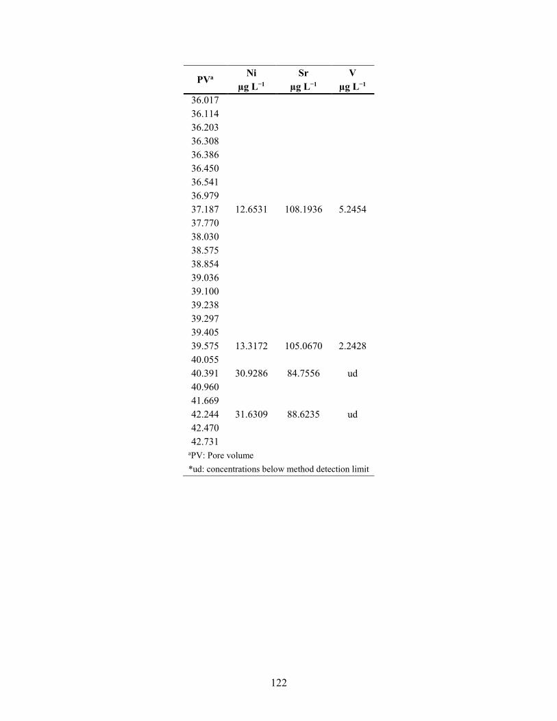
122
PVa Ni Sr V
µg L−1 µg L−1 µg L−1
36.017
36.114
36.203
36.308
36.386
36.450
36.541
36.979
37.187 12.6531 108.1936 5.2454
37.770
38.030
38.575
38.854
39.036
39.100
39.238
39.297
39.405
39.575 13.3172 105.0670 2.2428
40.055
40.391 30.9286 84.7556 ud
40.960
41.669
42.244 31.6309 88.6235 ud
42.470
42.731 aPV: Pore volume
*ud: concentrations below method detection limit

123
Table G.4. Measurements performed on the large column effluent.
PVa pH Eh ECb
(µS cm−1)
Alkalinity
(mg L−1)
0.01 5.22 500.89 1227.00 84.00
0.10 5.25 479.02 1348.00 83.67
0.19 5.23 442.11 1225.00 83.50
0.28 5.33 435.94 1083.00 87.13
0.37 5.37 418.12 1120.00 91.09
0.46 5.25 417.41 926.00 85.49
0.59 5.34 419.85 718.00 81.35
0.65 5.35 419.15 757.00 85.83
1.12 5.15 469.29 296.90 69.72
1.29 5.53 512.02 235.40 63.87
1.48 5.07 445.32 228.00 63.49
1.66 5.15 424.22 218.60 57.88
2.03 5.10 440.19 158.80 61.51
2.40 4.95 470.23 124.10 47.62
3.03 4.94 480.01 96.50 37.85
3.14 4.89 483.38 93.10 39.76
3.48 4.85 474.63 87.80 33.80
3.84 4.91 486.47 80.00 32.00
4.04 4.95 517.04 107.90 30.00
4.74 4.94 453.30 211.40 33.86
5.11 4.86 491.81 212.10 27.83
5.72 4.97 539.09 209.00 28.00
6.62 4.84 539.00 115.00 26.00
7.44 4.66 554.83 58.00 25.84
8.36 4.67 597.94 57.60 31.75
8.91 4.73 573.64 56.80 23.76
10.28 4.75 577.86 55.70 21.78
11.20 4.62 566.42 52.90 21.87
11.84 4.64 602.83 48.50 15.87
12.51 4.71 594.49 46.60 27.72
12.78 4.85 623.19 45.90 25.84
12.94 4.55 616.92 46.20 23.90
13.24 5.88 533.14 4000.00 485.15
13.31 6.10 447.81 4480.00 640.72
13.41 6.15 534.82 4650.00 641.43
13.69 6.10 485.36 4720.00 683.17
13.96 6.12 494.03 4720.00 657.37

124
PVa pH Eh ECb
(µS cm−1)
Alkalinity
(mg L−1)
14.50 6.16 468.38 4690.00 695.83
15.06 6.13 431.65 4670.00 693.84
15.87 6.20 418.43 4880.00 684.63
17.40 6.18 441.83 4840.00 710.32
18.23 6.34 514.96 4740.00 703.19
18.56 6.31 493.49 4760.00 709.16
19.11 6.35 484.76 4740.00 699.60
19.77 6.36 479.85 4890.00 695.83
20.13 6.50 461.56 4760.00 709.16
20.23 6.43 506.89 4820.00 706.00
20.48 6.45 417.72 4830.00 697.21
20.88 6.46 374.76 4810.00 660.00
21.87 6.45 418.79 4840.00 618.76
22.23 6.37 397.55 4810.00 695.83
22.88 6.65 441.53 4750.00 632.41
23.41 6.69 412.91 4670.00 738.52
23.94 6.80 489.88 4610.00 657.64
24.98 6.75 520.22 4230.00 758.48
25.79 6.72 519.11 4280.00 860.00
26.22 6.60 328.04 5060.00 934.39
26.39 6.96 343.00 5040.00 909.68
26.67 6.95 325.73 5010.00 914.51
26.76 6.86 457.34 4980.00 912.35
27.03 7.07 425.19 5010.00 894.21
27.65 7.08 490.25 4910.00 914.51
28.31 6.74 429.13 4900.00 906.93
28.96 6.72 484.11 4850.00 892.86
29.59 6.81 508.03 4820.00 876.49
30.20 6.72 499.02 4790.00 892.00
30.84 6.61 496.90 2765.00 701.79
31.46 6.35 386.29 965.00 180.87
31.95 6.00 474.25 534.00 101.39
32.10 6.01 452.24 460.00 79.37
32.47 6.15 460.32 380.00 64.53
32.76 6.49 472.39 308.00 51.69
33.38 5.61 458.26 103.60 41.75
33.61 5.54 460.54 86.00 35.76
33.74 5.48 466.83 68.00 27.78
34.02 5.61 470.56 54.20 27.83
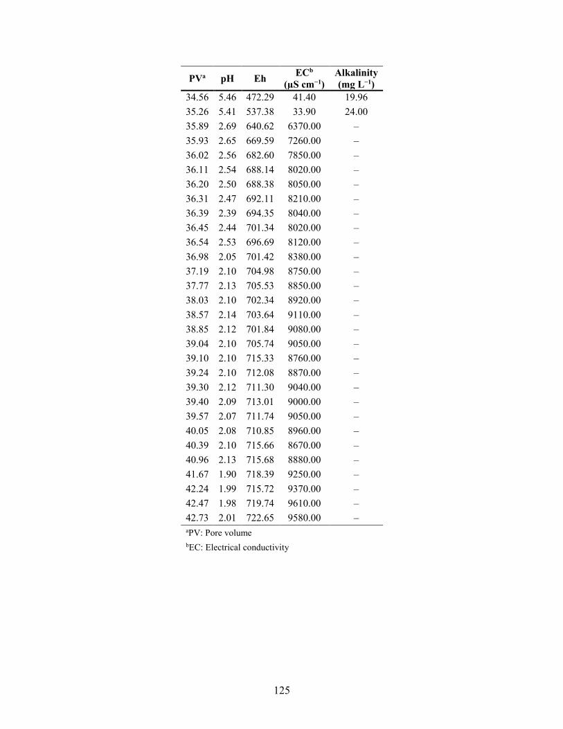
125
PVa pH Eh ECb
(µS cm−1)
Alkalinity
(mg L−1)
34.56 5.46 472.29 41.40 19.96
35.26 5.41 537.38 33.90 24.00
35.89 2.69 640.62 6370.00 –
35.93 2.65 669.59 7260.00 –
36.02 2.56 682.60 7850.00 –
36.11 2.54 688.14 8020.00 –
36.20 2.50 688.38 8050.00 –
36.31 2.47 692.11 8210.00 –
36.39 2.39 694.35 8040.00 –
36.45 2.44 701.34 8020.00 –
36.54 2.53 696.69 8120.00 –
36.98 2.05 701.42 8380.00 –
37.19 2.10 704.98 8750.00 –
37.77 2.13 705.53 8850.00 –
38.03 2.10 702.34 8920.00 –
38.57 2.14 703.64 9110.00 –
38.85 2.12 701.84 9080.00 –
39.04 2.10 705.74 9050.00 –
39.10 2.10 715.33 8760.00 –
39.24 2.10 712.08 8870.00 –
39.30 2.12 711.30 9040.00 –
39.40 2.09 713.01 9000.00 –
39.57 2.07 711.74 9050.00 –
40.05 2.08 710.85 8960.00 –
40.39 2.10 715.66 8670.00 –
40.96 2.13 715.68 8880.00 –
41.67 1.90 718.39 9250.00 –
42.24 1.99 715.72 9370.00 –
42.47 1.98 719.74 9610.00 –
42.73 2.01 722.65 9580.00 – aPV: Pore volume
bEC: Electrical conductivity

126
Table G.5. Major cations concentrations in the large column effluent quantified with inductively
coupled plasma–optical emission spectroscopy (ICP-OES).
PVa Ca
mg L−1
Fe
mg L−1
K
mg L−1
Mg
mg L−1
Na
mg L−1
S
mg L−1
0.01 151.4 3.0 13.4 44.9 30.0 182.5
0.10 178.4 4.1 15.1 57.7 33.3 239.1
0.19 160.9 4.0 11.7 56.7 31.0 228.8
0.28
0.37 133.9 3.8 8.8 47.0 24.3 183.1
0.46
0.59 79.8 5.2 5.2 27.6 14.7 99.9
0.65 87.4 4.3 5.7 25.4 15.2 93.6
1.12
1.29 18.5 15.3 1.1 5.4 4.8 15.8
1.48
1.66
2.03 9.1 17.3 0.5 2.5 3.7 5.6
2.40 6.0 16.8 0.4 1.4 3.5 2.6
3.03 4.2 12.5 0.3 0.9 3.4 2.0
3.14 4.1 11.9 0.3 1.0 3.6 2.1
3.48 3.5 10.3 0.3 0.9 3.6 2.0
3.84 3.1 9.4 0.3 0.8 3.3 1.6
4.04 2.8 8.8 0.3 0.8 9.7 1.7
4.74 2.3 7.7 0.3 0.7 29.2 1.5
5.11 2.1 7.6 0.3 0.6 29.3 1.3
5.72 1.8 0.0 0.3 0.0 30.4 0.1
6.62
7.44 1.3 4.9 0.2 0.4 3.2 0.9
8.36 1.1 0.0 0.2 0.0 3.5 0.1
8.91
10.28
11.20
11.84 0.7 2.7 0.1 0.2 3.6 1.0
12.51 0.6 2.6 0.1 0.2 3.5 1.0
12.78 0.6 2.5 ud 0.3 2.1 3.0
12.94 0.6 2.4 ud 0.3 2.1 3.2
13.24 0.5 0.2 12.6 5.7 939.1 73.4
13.31 0.7 0.2 17.1 13.0 1044.0 75.3
13.41 1.4 0.1 20.0 16.3 1104.2 75.0
13.69 2.6 0.1 23.0 18.3 1130.7 77.5
13.96 2.8 0.1 21.7 18.4 1115.0 73.2
14.50
15.06

127
PVa Ca
mg L−1
Fe
mg L−1
K
mg L−1
Mg
mg L−1
Na
mg L−1
S
mg L−1
15.87 5.3 0.8 21.9 20.2 1111.4 84.4
17.40 8.6 0.4 22.2 20.6 1116.2 85.0
18.23
18.56 6.1 0.4 22.1 19.9 1109.9 85.9
19.11
19.77 6.4 0.2 21.4 18.4 1027.0 75.7
20.13
20.23
20.48
20.88
21.87 5.5 0.4 21.1 19.3 1052.2 74.9
22.23
22.88
23.41
23.94 5.5 0.1 20.9 18.2 1052.0 74.6
24.98 4.3 0.2 20.4 17.9 1072.6 94.1
25.79
26.22 5.8 0.2 13.2 6.8 1168.3 205.1
26.39 5.8 0.3 13.2 6.9 1195.2 206.1
26.67 5.9 0.3 12.9 6.7 1179.2 204.8
26.76
27.03
27.65 5.9 0.2 12.9 6.7 1207.0 202.4
28.31
28.96
29.59 6.1 0.1 12.6 6.7 1200.4 203.2
30.20
30.84
31.46
31.95
32.10
32.47 3.8 ud* ud 0.7 61.5 8.7
32.76
33.38
33.61 2.7 ud ud 0.6 9.8 3.9
33.74
34.02
34.56
35.26
35.89 331.4 2141.0 5.2 154.1 143.8 2610.0
35.93 387.9 2592.4 5.5 193.0 188.5 3236.5

128
PVa Ca
mg L−1
Fe
mg L−1
K
mg L−1
Mg
mg L−1
Na
mg L−1
S
mg L−1
36.02 408.1 2944.2 4.2 206.1 206.7 3647.0
36.11 415.1 2973.2 2.2 210.0 215.6 3607.9
36.20 415.4 2831.6 ud 194.5 199.0 3372.7
36.31
36.39 418.7 2787.9 ud 193.4 197.1 3396.9
36.45 421.6 2772.8 ud 192.4 196.6 3386.6
36.54 406.7 2906.8 0.2 204.6 207.4 3665.2
36.98 423.8 2754.1 ud 191.3 194.5 3385.2
37.19 400.2 2874.2 0.0 208.6 214.7 3665.4
37.77
38.03 428.0 2777.9 ud 193.3 191.7 3473.1
38.57 430.6 2786.9 ud 194.8 193.3 3571.6
38.85 400.6 2856.7 ud 209.5 215.7 3703.5
39.04
39.10
39.24 391.2 2792.3 ud 206.3 209.8 3591.1
39.30
39.40
39.57 391.0 2838.9 ud 204.6 212.7 3567.3
40.05
40.39 417.0 2723.8 ud 195.4 197.9 3568.7
40.96
41.67 409.3 2692.1 ud 202.1 204.8 3738.7
42.24 407.8 2458.8 ud 202.9 208.5 3759.2
42.47
42.73 414.7 2625.6 ud 207.3 219.3 3489.1 aPV: Pore volume
*ud: concentrations below method detection limit

129
Table G.6. Trace elements concentrations in the large column effluent quantified with inductively
coupled plasma–optical mass spectroscopy (ICP-MS).
PVa Al Ca Fe K Mg Mo
µg L−1 µg L−1 µg L−1 µg L−1 µg L−1 µg L−1
0.01 105.48 147174.26 3370.9 11090.4 54234.3 1.48
0.10 128.61 175767.97 4329.6 12275.2 64847.1 0.93
0.19 110.72 157206.82 4327.5 10696.4 57978.2 1.42
0.28 99.53 139058.44 3935.7 9409.1 51054.1 1.33
0.37 106.81 139343.60 4226.1 8907.9 51086.6 1.75
0.46
0.59 104.76 82753.74 5596.5 5081.8 30322.3 1.34
0.65
1.12
1.29 108.43 18247.19 17100.3 1007.0 6367.7 ud
1.48
1.66
2.03
2.40 149.46 6039.99 18089.4 381.7 1608.0 ud
3.03
3.14
3.48
3.84 328.72 3030.63 10459.2 260.3 911.0 ud
4.04
4.74
5.11
5.72
6.62
7.44 936.88 1379.98 5217.4 160.8 475.8 ud
8.36
8.91
10.28
11.20
11.84 657.72 363.27 2600.4 134.2 254.9 0.93
12.51 632.51 378.25 2765.6 184.1 297.1 3.50
12.78 797.90 778.87 2784.3 134.5 282.3 ud
12.94 800.76 765.27 2666.6 131.4 269.4 ud
13.24 ud ud 184.9 11592.4 6057.3 556.90
13.31 ud 383.90 87.0 16006.5 14918.1 574.42
13.41 ud 1200.01 96.2 18350.0 17952.0 396.36
13.69 ud 2492.35 102.8 19901.5 19595.3 171.25
13.96 ud 2565.00 149.9 20224.2 20309.7 113.47
14.50

130
PVa Al Ca Fe K Mg Mo
µg L−1 µg L−1 µg L−1 µg L−1 µg L−1 µg L−1
15.06
15.87 ud 6104.22 939.0 18027.2 22537.0 43.68
17.40
18.23
18.56 ud 6980.80 469.6 18107.0 22490.6 23.65
19.11
19.77 ud 6448.92 174.4 20747.7 20987.7 21.10
20.13
20.23
20.48
20.88
21.87 ud 5494.52 469.1 21039.5 22499.2 16.85
22.23
22.88
23.41
23.94 ud 6594.25 213.4 21258.3 21687.4 13.62
24.98 ud 4029.14 175.1 20528.1 20641.2 18.51
25.79
26.22 81.23 5604.07 276.3 11735.4 6809.2 146.96
26.39 87.59 5840.90 250.7 11666.6 6750.8 152.46
26.67 84.66 5675.93 322.0 11814.0 6725.4 152.86
26.76
27.03
27.65 71.04 6070.23 279.1 11380.1 6822.2 145.49
28.31
28.96
29.59 33.35 5728.02 115.5 11536.9 6555.9 144.10
30.20
30.84 49.73 3916.55 387.2 6824.7 4045.6 57.54
31.46
31.95
32.10
32.47 ud 4149.70 18.8 612.2 868.1 3.80
32.76 ud 3780.51 15.3 603.7 817.5 3.12
33.38
33.61 ud 2734.47 ud 216.7 532.8 ud
33.74
34.02
34.56
35.26
35.89 111282.08 333392.51 2125587.9 5333.4 138717.8 106.67
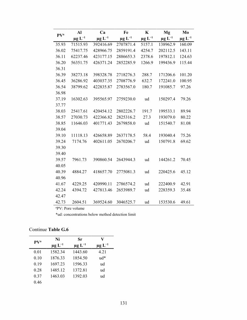
131
PVa Al Ca Fe K Mg Mo
µg L−1 µg L−1 µg L−1 µg L−1 µg L−1 µg L−1
35.93 71515.93 392416.69 2707871.4 5157.1 138962.9 160.09
36.02 75417.75 428966.75 2859191.4 4254.7 202112.5 143.11
36.11 62237.46 423177.15 2886653.3 2378.6 197812.1 124.63
36.20 56351.75 426371.24 2852285.9 1266.9 199436.9 115.44
36.31
36.39 38273.18 398328.78 2718276.3 288.7 171206.6 101.20
36.45 36286.92 403037.35 2708776.9 632.7 172241.0 100.95
36.54 38799.62 422835.87 2783567.0 180.7 191085.7 97.26
36.98
37.19 16302.63 395565.97 2759230.0 ud 150297.4 79.26
37.77
38.03 25417.61 420454.12 2802226.7 191.7 199533.1 89.94
38.57 27030.73 422366.82 2825316.2 27.3 193079.0 80.22
38.85 11646.03 401771.43 2679858.0 ud 151540.7 81.08
39.04
39.10 11118.13 426658.89 2637178.5 58.4 193040.4 75.26
39.24 7174.76 402611.05 2670206.7 ud 150791.8 69.62
39.30
39.40
39.57 7961.73 390860.54 2643944.3 ud 144261.2 70.45
40.05
40.39 4884.27 418657.70 2775081.3 ud 220425.6 45.12
40.96
41.67 4229.25 420990.11 2786574.2 ud 222400.9 42.91
42.24 4394.72 427813.46 2653989.7 ud 228359.3 35.48
42.47
42.73 2604.51 369524.60 3046525.7 ud 153530.6 49.61 aPV: Pore volume
*ud: concentrations below method detection limit
Continue Table G.6
PVa Ni Sr V
µg L−1 µg L−1 µg L−1
0.01 1582.34 1443.60 4.21
0.10 1876.33 1854.50 ud*
0.19 1697.23 1596.33 ud
0.28 1485.12 1372.81 ud
0.37 1463.03 1392.03 ud
0.46

132
PVa Ni Sr V
µg L−1 µg L−1 µg L−1
0.59 866.00 853.18 ud
0.65
1.12
1.29 205.88 236.83 ud
1.48
1.66
2.03
2.40 58.48 64.28 ud
3.03
3.14
3.48
3.84 27.30 29.71 ud
4.04
4.74
5.11
5.72
6.62
7.44 16.71 16.36 2.24
8.36
8.91
10.28
11.20
11.84 7.76 9.94 4.69
12.51 9.67 10.20 7.40
12.78 8.50 10.12 7.35
12.94 9.34 10.08 7.62
13.24 ud 13.04 61.02
13.31 ud 16.61 68.91
13.41 ud 22.95 86.19
13.69 ud 22.54 97.91
13.96 ud 16.38 97.70
14.50
15.06
15.87 ud 9.84 16.87
17.40
18.23
18.56 ud 7.86 8.90
19.11
19.77 ud 7.44 6.08
20.13
20.23

133
PVa Ni Sr V
µg L−1 µg L−1 µg L−1
20.48
20.88
21.87 ud 6.72 6.11
22.23
22.88
23.41
23.94 ud 8.14 5.38
24.98 ud 4.69 5.90
25.79
26.22 5.29 272.34 21.66
26.39 ud 300.67 19.33
26.67 5.09 321.13 20.44
26.76
27.03
27.65 4.76 351.65 20.47
28.31
28.96
29.59 5.58 362.78 31.72
30.20
30.84 ud 228.55 20.46
31.46
31.95
32.10
32.47 ud 123.38 ud
32.76 ud 123.56 ud
33.38
33.61 ud 51.96 ud
33.74
34.02
34.56
35.26
35.89 2303.04 793.10 6904.08
35.93 2070.21 782.08 4618.69
36.02 1581.94 645.33 3477.44
36.11 1319.45 572.96 2997.98
36.20 1175.69 535.82 2796.60
36.31
36.39 882.69 481.01 2341.73
36.45 822.43 461.52 2259.74
36.54 766.79 399.60 2265.99
36.98

134
PVa Ni Sr V
µg L−1 µg L−1 µg L−1
37.19 462.87 259.56 1555.83
37.77
38.03 664.99 213.00 2073.32
38.57 750.64 236.13 1840.40
38.85 576.51 171.88 1158.85
39.04
39.10 374.86 137.91 884.78
39.24 249.93 123.37 750.91
39.30
39.40
39.57 145.20 137.06 945.96
40.05
40.39 62.40 75.49 379.19
40.96
41.67 83.74 105.05 475.23
42.24 85.70 106.27 367.66
42.47
42.73 78.09 104.60 414.89 aPV: Pore volume
*ud: concentrations below method detection limit
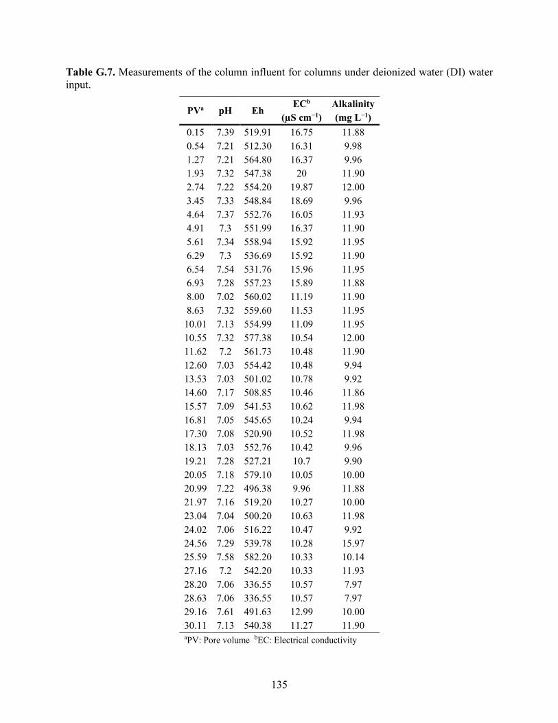
135
Table G.7. Measurements of the column influent for columns under deionized water (DI) water
input.
PVa pH Eh ECb Alkalinity
(µS cm−1) (mg L−1)
0.15 7.39 519.91 16.75 11.88
0.54 7.21 512.30 16.31 9.98
1.27 7.21 564.80 16.37 9.96
1.93 7.32 547.38 20 11.90
2.74 7.22 554.20 19.87 12.00
3.45 7.33 548.84 18.69 9.96
4.64 7.37 552.76 16.05 11.93
4.91 7.3 551.99 16.37 11.90
5.61 7.34 558.94 15.92 11.95
6.29 7.3 536.69 15.92 11.90
6.54 7.54 531.76 15.96 11.95
6.93 7.28 557.23 15.89 11.88
8.00 7.02 560.02 11.19 11.90
8.63 7.32 559.60 11.53 11.95
10.01 7.13 554.99 11.09 11.95
10.55 7.32 577.38 10.54 12.00
11.62 7.2 561.73 10.48 11.90
12.60 7.03 554.42 10.48 9.94
13.53 7.03 501.02 10.78 9.92
14.60 7.17 508.85 10.46 11.86
15.57 7.09 541.53 10.62 11.98
16.81 7.05 545.65 10.24 9.94
17.30 7.08 520.90 10.52 11.98
18.13 7.03 552.76 10.42 9.96
19.21 7.28 527.21 10.7 9.90
20.05 7.18 579.10 10.05 10.00
20.99 7.22 496.38 9.96 11.88
21.97 7.16 519.20 10.27 10.00
23.04 7.04 500.20 10.63 11.98
24.02 7.06 516.22 10.47 9.92
24.56 7.29 539.78 10.28 15.97
25.59 7.58 582.20 10.33 10.14
27.16 7.2 542.20 10.33 11.93
28.20 7.06 336.55 10.57 7.97
28.63 7.06 336.55 10.57 7.97
29.16 7.61 491.63 12.99 10.00
30.11 7.13 540.38 11.27 11.90 aPV: Pore volume bEC: Electrical conductivity

136
Table G.8. Major cation concentrations quantified with inductively coupled plasma–optical
emission spectroscopy (ICP-OES) in the influent columns during deionized water (DI) input.
PVa Ca Fe K Mg Na S
mg L−1 mg L−1 mg L−1 mg L−1 mg L−1 mg L−1
0.15 0.1076 0.0008 ud* ud 3.6425 0.1406
0.54
1.27
1.93
2.74
3.45 ud ud ud ud 4.1461 0.2306
4.64 0.3086 ud ud 0.0222 3.452 0.1797
4.91
5.61
6.29
6.54
6.93
8.00
8.63 ud ud ud 0.0526 2.3465 ud
10.01
10.55
11.62
12.60
13.53
14.60
15.57
16.81 ud ud ud 0.024 2.0431 ud
17.30
18.13
19.21
20.05
20.99
21.97
23.04
24.02
24.56 0.1801 1.7124 ud 0.0413 2.1644 0.9162
25.59
27.16
28.20
28.63
29.16
30.11
aPV: Pore volume *ud: concentrations below method detection limit
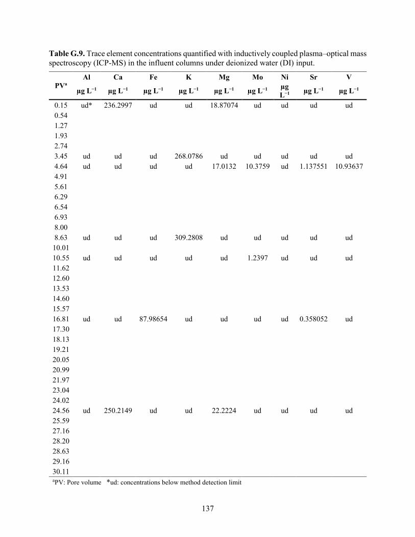
137
Table G.9. Trace element concentrations quantified with inductively coupled plasma–optical mass
spectroscopy (ICP-MS) in the influent columns under deionized water (DI) input.
PVa
Al Ca Fe K Mg Mo Ni Sr V
µg L−1 µg L−1 µg L−1 µg L−1 µg L−1 µg L−1 µg
L−1 µg L−1 µg L−1
0.15 ud* 236.2997 ud ud 18.87074 ud ud ud ud
0.54
1.27
1.93
2.74
3.45 ud ud ud 268.0786 ud ud ud ud ud
4.64 ud ud ud ud 17.0132 10.3759 ud 1.137551 10.93637
4.91
5.61
6.29
6.54
6.93
8.00
8.63 ud ud ud 309.2808 ud ud ud ud ud
10.01
10.55 ud ud ud ud ud 1.2397 ud ud ud
11.62
12.60
13.53
14.60
15.57
16.81 ud ud 87.98654 ud ud ud ud 0.358052 ud
17.30
18.13
19.21
20.05
20.99
21.97
23.04
24.02
24.56 ud 250.2149 ud ud 22.2224 ud ud ud ud
25.59
27.16
28.20
28.63
29.16
30.11 aPV: Pore volume *ud: concentrations below method detection limit
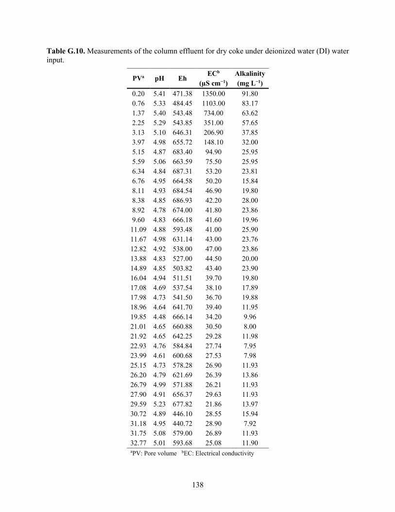
138
Table G.10. Measurements of the column effluent for dry coke under deionized water (DI) water
input.
PVa pH Eh ECb Alkalinity
(µS cm−1) (mg L−1)
0.20 5.41 471.38 1350.00 91.80
0.76 5.33 484.45 1103.00 83.17
1.37 5.40 543.48 734.00 63.62
2.25 5.29 543.85 351.00 57.65
3.13 5.10 646.31 206.90 37.85
3.97 4.98 655.72 148.10 32.00
5.15 4.87 683.40 94.90 25.95
5.59 5.06 663.59 75.50 25.95
6.34 4.84 687.31 53.20 23.81
6.76 4.95 664.58 50.20 15.84
8.11 4.93 684.54 46.90 19.80
8.38 4.85 686.93 42.20 28.00
8.92 4.78 674.00 41.80 23.86
9.60 4.83 666.18 41.60 19.96
11.09 4.88 593.48 41.00 25.90
11.67 4.98 631.14 43.00 23.76
12.82 4.92 538.00 47.00 23.86
13.88 4.83 527.00 44.50 20.00
14.89 4.85 503.82 43.40 23.90
16.04 4.94 511.51 39.70 19.80
17.08 4.69 537.54 38.10 17.89
17.98 4.73 541.50 36.70 19.88
18.96 4.64 641.70 39.40 11.95
19.85 4.48 666.14 34.20 9.96
21.01 4.65 660.88 30.50 8.00
21.92 4.65 642.25 29.28 11.98
22.93 4.76 584.84 27.74 7.95
23.99 4.61 600.68 27.53 7.98
25.15 4.73 578.28 26.90 11.93
26.20 4.79 621.69 26.39 13.86
26.79 4.99 571.88 26.21 11.93
27.90 4.91 656.37 29.63 11.93
29.59 5.23 677.82 21.86 13.97
30.72 4.89 446.10 28.55 15.94
31.18 4.95 440.72 28.90 7.92
31.75 5.08 579.00 26.89 11.93
32.77 5.01 593.68 25.08 11.90 aPV: Pore volume bEC: Electrical conductivity

139
Table G.11. Major cation concentrations quantified with inductively coupled plasma–optical
emission spectroscopy (ICP-OES) in the effluent from the column with dry coke during
deionized water (DI) input
PVa Ca Fe K Mg Na S
mg L−1 mg L−1 mg L−1 mg L−1 mg L−1 mg L−1
0.20 153.098 1.1411 9.6767 44.1964 28.1859 205.017
0.76 140.019 0.5048 7.9509 41.4668 23.9898 186.269
1.37 85.8402 0.3654 4.7538 25.7821 15.02 113.067
2.25 36.4146 0.2561 1.9085 10.5747 7.6783 44.4198
3.13 17.0934 ud* 0.8759 4.4216 6.4193 17.5751
3.97 9.3372 ud 0.4641 2.2264 4.6375 8.9647
5.15 3.3758 ud 0.1974 0.6916 4.4756 3.6988
5.59
6.34
6.76 2.6308 ud 0.1303 0.4088 3.5496 2.5744
8.11
8.38 1.6797 ud 0.1006 0.3155 3.4499 2.1819
8.92
9.60 1.3988 ud 0.0918 0.2804 3.4733 1.9751
11.09
11.67
12.82
13.88
14.89
16.04
17.08
17.98 0.6661 2.6919 0.0648 0.1544 2.145 1.1382
18.96
19.85
21.01
21.92
22.93
23.99
25.15
26.20
26.79 0.4741 1 0.0589 0.0861 2.0357 0.9352
27.90
29.59
30.72
31.18
31.75
32.77

140
PVa Ca Fe K Mg Na S
mg L−1 mg L−1 mg L−1 mg L−1 mg L−1 mg L−1 aPV: Pore volume *ud: concentrations below method detection limit
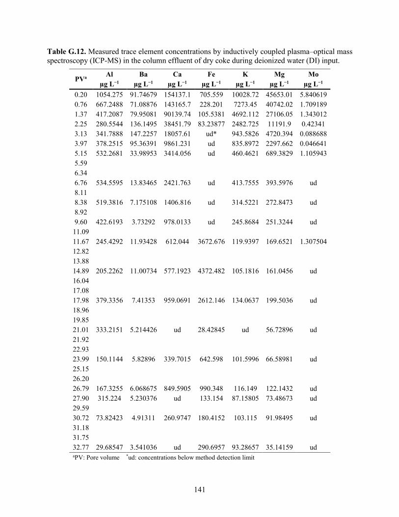
141
Table G.12. Measured trace element concentrations by inductively coupled plasma–optical mass
spectroscopy (ICP-MS) in the column effluent of dry coke during deionized water (DI) input.
PVa Al Ba Ca Fe K Mg Mo
µg L−1 µg L−1 µg L−1 µg L−1 µg L−1 µg L−1 µg L−1
0.20 1054.275 91.74679 154137.1 705.559 10028.72 45653.01 5.840619
0.76 667.2488 71.08876 143165.7 228.201 7273.45 40742.02 1.709189
1.37 417.2087 79.95081 90139.74 105.5381 4692.112 27106.05 1.343012
2.25 280.5544 136.1495 38451.79 83.23877 2482.725 11191.9 0.42341
3.13 341.7888 147.2257 18057.61 ud* 943.5826 4720.394 0.088688
3.97 378.2515 95.36391 9861.231 ud 835.8972 2297.662 0.046641
5.15 532.2681 33.98953 3414.056 ud 460.4621 689.3829 1.105943
5.59
6.34
6.76 534.5595 13.83465 2421.763 ud 413.7555 393.5976 ud
8.11
8.38 519.3816 7.175108 1406.816 ud 314.5221 272.8473 ud
8.92
9.60 422.6193 3.73292 978.0133 ud 245.8684 251.3244 ud
11.09
11.67 245.4292 11.93428 612.044 3672.676 119.9397 169.6521 1.307504
12.82
13.88
14.89 205.2262 11.00734 577.1923 4372.482 105.1816 161.0456 ud
16.04
17.08
17.98 379.3356 7.41353 959.0691 2612.146 134.0637 199.5036 ud
18.96
19.85
21.01 333.2151 5.214426 ud 28.42845 ud 56.72896 ud
21.92
22.93
23.99 150.1144 5.82896 339.7015 642.598 101.5996 66.58981 ud
25.15
26.20
26.79 167.3255 6.068675 849.5905 990.348 116.149 122.1432 ud
27.90 315.224 5.230376 ud 133.154 87.15805 73.48673 ud
29.59
30.72 73.82423 4.91311 260.9747 180.4152 103.115 91.98495 ud
31.18
31.75
32.77 29.68547 3.541036 ud 290.6957 93.28657 35.14159 ud aPV: Pore volume *ud: concentrations below method detection limit
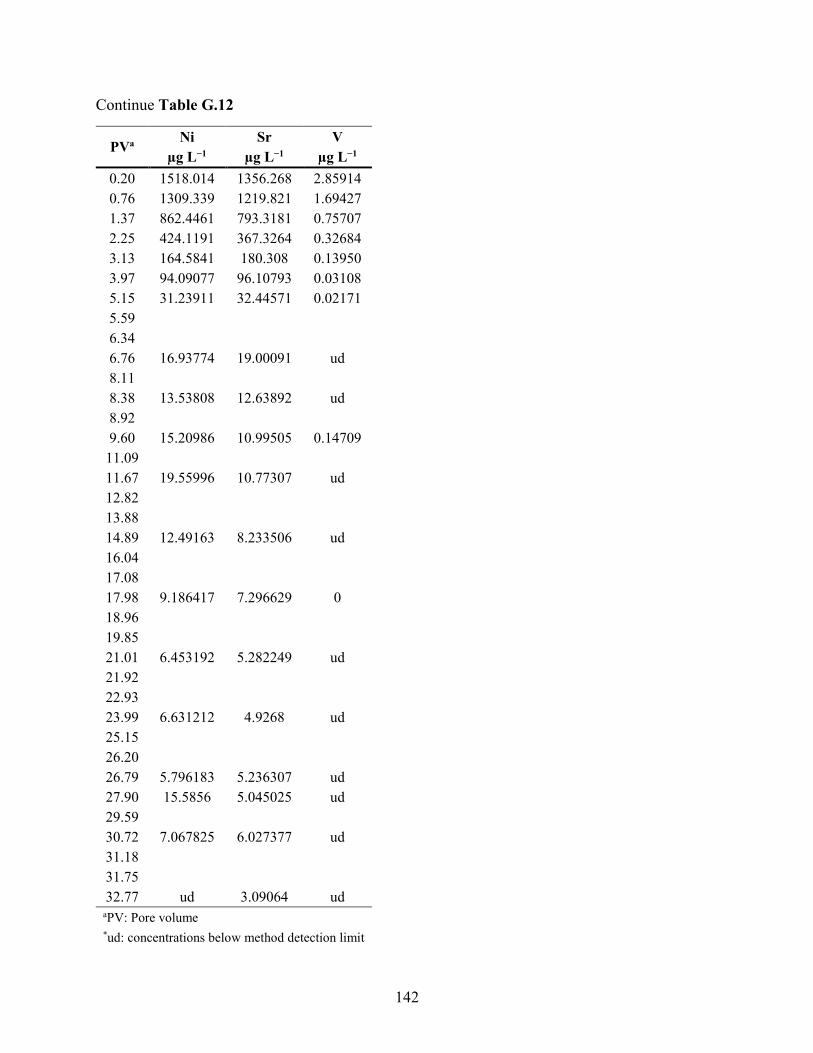
142
Continue Table G.12
PVa Ni Sr V
µg L−1 µg L−1 µg L−1
0.20 1518.014 1356.268 2.85914
0.76 1309.339 1219.821 1.69427
1.37 862.4461 793.3181 0.75707
2.25 424.1191 367.3264 0.32684
3.13 164.5841 180.308 0.13950
3.97 94.09077 96.10793 0.03108
5.15 31.23911 32.44571 0.02171
5.59
6.34
6.76 16.93774 19.00091 ud
8.11
8.38 13.53808 12.63892 ud
8.92
9.60 15.20986 10.99505 0.14709
11.09
11.67 19.55996 10.77307 ud
12.82
13.88
14.89 12.49163 8.233506 ud
16.04
17.08
17.98 9.186417 7.296629 0
18.96
19.85
21.01 6.453192 5.282249 ud
21.92
22.93
23.99 6.631212 4.9268 ud
25.15
26.20
26.79 5.796183 5.236307 ud
27.90 15.5856 5.045025 ud
29.59
30.72 7.067825 6.027377 ud
31.18
31.75
32.77 ud 3.09064 ud aPV: Pore volume *ud: concentrations below method detection limit

143
Table G.13. Measurements of the column effluent for the slurry coke during deionized water (DI)
input.
PVa pH Eh ECb
(µS cm−1)
Alkalinity
(mg L−1)
0.15 6.23 498.13 2623 633.66
0.54 6.17 437.60 1873 524.00
1.27 6.36 546.75 1346 474.00
1.93 6.16 490.01 1064 358.00
2.74 5.92 544.21 721 318.73
3.45 5.9 517.62 524 188.87
4.64 5.51 498.64 266 86.00
4.91 5.8 490.80 250.8 95.24
5.61 5.17 534.15 115.8 49.90
6.29 5.08 515.33 81.5 37.77
6.54 4.96 509.32 75.4 29.94
6.93 5.13 546.32 75.6 35.71
8.00 4.98 565.11 60 25.64
8.63 5 590.58 60.2 25.69
10.01 4.85 543.20 55.8 27.61
10.55 4.98 619.88 54.3 26.00
11.62 4.9 566.13 52.1 27.72
12.60 4.78 536.01 51.6 19.65
13.53 4.85 493.21 52.1 25.95
14.60 4.86 511.82 51.3 27.72
15.57 4.77 516.84 50.6 27.83
16.81 4.97 557.84 48.4 28.35
17.30 5.02 539.31 41.9 27.94
18.13 4.8 550.25 37.3 21.87
19.21 4.86 539.70 38.4 19.80
20.05 4.9 538.78 36.9 11.93
20.99 4.94 511.24 35.6 19.96
21.97 4.75 551.75 34.3 19.76
23.04 4.77 546.80 33.2 17.96
24.02 4.92 561.91 31.9 23.76
24.56 5.18 541.22 29.55 21.83
25.59 5.01 583.05 34.9 20.87
27.16 5.17 605.01 24.27 21.87
28.20 5.05 429.48 31.3 9.94
28.63 4.99 415.66 30.9 15.84
29.16 5.16 543.64 28.58 17.89
30.11 5.09 554.70 28.81 15.94 aPV: Pore volume bEC: Electrical conductivity

144
Table G.14. Major cation concentrations quantified with inductively coupled plasma–optical
emission spectroscopy (ICP-OES) in the effluent of the column with slurry coke during deionized
water (DI) input.
PVa Ca Fe K Mg Na S
mg L−1 mg L−1 mg L−1 mg L−1 mg L−1 mg L−1
0.15 118.138 0.0096 18.6966 39.6136 478.885 128.645
0.54 92.139 0.0632 12.7794 25.0059 292.136 72.6721
1.27 67.1619 0.0583 9.3507 19.665 197.916 52.4042
1.93 52.8426 0.024 6.9687 15.4788 141.058 38.7931
2.74 44.7308 0.0618 4.384 13.2805 73.9878 22.4317
3.45 36.922 0.1263 4.5081 10.4282 42.058 14.8552
4.64 15.0576 1.2333 2.0291 3.5237 14.686 4.7629
4.91 18.2035 0.9032 2.4726 4.3124 20.57 6.8061
5.61
6.29 4.0144 4.1782 0.7669 0.6718 4.86 1.0312
6.54
6.93 2.8672 5.1197 0.6114 0.512 4.6385 0.8882
8.00
8.63 2.4321 2.5611 0.5461 0.4007 4.3777 0.7749
10.01
10.55 1.8311 3.9294 0.4061 0.2925 3.0917 0.4205
11.62
12.60
13.53 1.337 4.4143 0.3285 0.2318 2.8969 0.3447
14.60
15.57
16.81 1.2982 4.8224 0.2542 0.1917 2.3388 ud*
17.30
18.13
19.21 1.0412 1.7513 0.2698 0.1668 2.8423 0.5175
20.05
20.99
21.97
23.04
24.02
24.56 0.6739 1.6966 0.1854 0.1189 2.2889 ud
25.59 0.7791 0.5292 0.2423 0.131 2.77 0.5183
27.16
28.20 0.7374 0.789 0.3099 0.1946 3.0825 0.2291
28.63
29.16
30.11 0.52075 0.7419 0.18875 0.08945 2.99695 0.18805

145
PVa Ca Fe K Mg Na S
mg L−1 mg L−1 mg L−1 mg L−1 mg L−1 mg L−1 aPV: Pore volume *ud: concentrations below method detection limit

146
Table G.15. Measured trace element concentrations by inductively coupled plasma–optical mass
spectroscopy (ICP-MS) in the column effluent with slurry coke during deionized water (DI) input.
PVa Al Ba Ca Fe K Mg Mo
µg L−1 µg L−1 µg L−1 µg L−1 µg L−1 µg L−1 µg L−1
0.15 ud* 341.0929 126323.7244 47.4769 17346.9214 39114.3154 693.7751
0.54
1.27 ud 268.5195 76980.7550 78.8840 8728.0681 20876.8206 306.3904
1.93 ud 272.4810 57131.0877 40.8729 6507.5718 15821.1319 219.9579
2.74 ud 316.4384 48697.5861 70.0613 4214.0754 13775.3808 142.5299
3.45 9.1204 378.0643 40031.3614 140.7836 4306.2566 10734.3382 83.0690
4.64 237.6502 565.8068 16330.9556 1390.9374 1984.9616 3954.1621 22.1265
4.91 114.2764 592.2015 19887.8391 958.8048 2296.8779 4289.2272 27.5753
5.61
6.29 366.7105 304.6301 4154.7846 4657.9454 669.6022 681.8169 2.6033
6.54
6.93 355.1652 190.0017 2914.4741 5655.0260 577.7165 474.6586 1.3078
8.00
8.63 411.4080 112.3786 3166.6357 2746.3574 556.0781 371.4513 1.1242
10.01
10.55 469.2789 65.1652 1529.6811 4121.5779 385.9877 229.1018 0.9078
11.62
12.60
13.53 566.1211 39.6569 1392.1488 4954.5034 332.2235 220.9555 1.1583
14.60
15.57
16.81 748.1048 29.9156 1292.9647 3959.4417 292.2019 228.3194 ud
17.30
18.13
19.21 667.9247 23.1274 814.5564 1925.4341 280.3157 107.5349 1.5688
20.05
20.99
21.97 618.3642 17.9689 508.3928 1698.7350 240.2733 84.9139 2.5230
23.04
24.02
24.56 691.3165 15.2348 693.6084 1761.9543 236.6949 132.7037 ud
25.59 480.1833 15.8531 229.3530 609.2824 219.2522 61.8705 2.1172
27.16
28.20 263.8925 14.0889 536.6676 818.9251 267.1752 132.0911 1.2924
28.63
29.16
30.11 350.5555 10.7390 251.7175 772.0037 192.6040 33.8566 1.7714 aPV: Pore volume *ud: concentrations below method detection limit

147
Continue Table G.15
PVa Ni Sr V
µg L−1 µg L−1 µg L−1
0.15 107.6154 2993.4854 6759.3779
0.54
1.27 97.2664 1378.7967 2791.0315
1.93 99.6794 1003.7842 2098.8847
2.74 123.0122 896.5544 1352.2646
3.45 174.5479 673.2756 817.5767
4.64 654.5728 276.8757 273.3856
4.91 580.9526 302.2118 297.0199
5.61
6.29 284.8549 55.2044 53.9074
6.54
6.93 178.6023 41.5887 38.5921
8.00
8.63 109.1615 34.2211 24.7332
10.01
10.55 61.6328 25.4306 18.5820
11.62
12.60
13.53 45.8005 20.2658 11.0673
14.60 14.0000
15.57
16.81 35.5087 17.2071 14.2719
17.30
18.13
19.21 23.3730 13.0213 19.8938
20.05
20.99
21.97 16.9728 10.8099 17.3967
23.04
24.02
24.56 16.1193 9.1957 14.9984
25.59 30.6232 9.2272 19.4799
27.16
28.20 13.5086 11.6826 24.2236
28.63
29.16
30.11 9.7229 7.3844 20.1441 aPV: Pore volume
*ud: concentrations below method detection limit

148
Table G.16. Measurements of the columns influent during oil sand process-affected water
(OSPW) input.
PVa pH Eh ECb Alkalinity
(mS cm−1) (mg L−1)
0.18 8.57 475.91 4.9 726.73
0.44 8.52 429.81 4.88 706.35
0.62 8.47 465.99 4.86 704.37
1.42 8.61 446.45 4.85 707.75
1.94 8.61 485.42 4.84 709.16
2.48 8.76 436.54 4.81 712.30
3.31 8.74 436.88 4.83 710.89
3.58 8.82 424.39 4.81 714.00
4.43 8.75 416.85 4.77 694.44
5.39 8.79 416.36 4.72 715.14
6.67 8.81 463.04 4.7 714.57
7.63 8.82 408.30 4.93 712.87
8.73 8.8 454.52 4.81 716.57
9.73 8.4 443.80 4.88 718.56
10.42 8.46 439.85 4.8 710.58
11.51 8.5 430.00 4.78 713.72
12.36 8.48 465.86 4.75 703.19
13.47 8.55 468.22 4.89 714.00
14.34 8.42 523.75 4.86 738.52
15.30 8.28 480.84 4.86 718.56
16.31 8.35 436.95 4.83 714.29
17.41 8.36 412.28 4.83 734.13
18.41 8.39 419.42 4.78 695.83
19.10 8.24 456.18 4.73 714.29
20.04 8.5 534.30 4.66 732.60
21.64 8.5 534.30 4.66 732.60
22.72 8.74 449.94 4.92 710.32
23.16 8.74 449.94 4.92 710.32
23.70 9.03 387.33 4.86 711.46
24.68 9.01 353.59 4.88 694.44
25.43 8.59 361.33 4.92 718.56
26.42 8.76 467.14 4.84 712.00
27.40 8.88 412.93 4.81 708.58
28.34 8.79 475.83 4.84 717.06
29.32 8.95 469.82 4.88 704.37
30.28 8.35 432.01 4.76 712.87
31.26 8.54 469.56 5.05 705.18
32.29 8.69 488.76 4.93 702.97

149
PVa pH Eh ECb Alkalinity
(mS cm−1) (mg L−1)
33.24 8.45 435.36 4.92 691.70
34.21 8.59 506.78 4.88 674.60
35.06 8.45 435.36 4.92 691.70 aPV: Pore volume bEC: Electrical conductivity

150
Table G.17. Major cation concentrations quantified by inductively coupled plasma–optical
emission spectroscopy (ICP-OES) in the column influent during OSPW input.
PVa Ca Fe K Mg Na S
mg L−1 mg L−1 mg L−1 mg L−1 mg L−1 mg L−1
0.18
0.44
0.62 7.951 ud* 21.177 19.1367 1060.51 78.1026
1.42
1.94
2.48
3.31 6.4873 ud 21.5442 19.6679 1083.6 81.7178
3.58
4.43
5.39 6.5222 ud 20.9386 19.122 1062.27 79.2602
6.67
7.63
8.73
9.73
10.42 9.0037 ud 20.5862 17.9018 1009.6 71.6384
11.51
12.36
13.47
14.34
15.30
16.31
17.41
18.41
19.10 23.0997 ud 19.928 18.0666 1027.14 68.6614
20.04 17.0526 ud 21.5397 19.693 1075.49 80.4857
21.64
22.72
23.16
23.70
24.68
25.43
26.42
27.40
28.34
29.32
30.28
31.26
32.29

151
PVa Ca Fe K Mg Na S
mg L−1 mg L−1 mg L−1 mg L−1 mg L−1 mg L−1
33.24
34.21
35.06
aPV: Pore volume
*ud: concentrations below method detection limit

152
Table G.18. Trace element concentrations quantified by inductively coupled plasma–optical mass
spectroscopy (ICP-MS) in the column influent during oil sand process-affected water (OSPW)
input.
PVa Al Ba Ca Fe K Mg Mo
µg L−1 µg L−1 µg L−1 µg L−1 µg L−1 µg L−1 µg L−1
0.18 ud* ud 7680.8081 ud 19313.2812 17217.3055 1.2191
0.44
0.62 5.5114 ud 3584.6117 96.2101 19532.0560 16932.5115 ud
1.42 ud ud 8023.3107 ud 21188.5877 20071.8306 1.8669
1.94
2.48
3.31
3.58
4.43 ud ud 6647.8426 14.6264 18126.3398 20757.5417 12.1605
5.39 ud 1.4074 6210.5920 ud 20144.7347 19342.0296 1.8261
6.67
7.63
8.73
9.73
10.42 ud ud 9745.2377 3209.5717 17764.2946 18668.9361 ud
11.51
12.36
13.47
14.34
15.30
16.31
17.41 ud ud 6066.4407 81.2089 20305.2461 21241.3084 1.1853
18.41
19.10 ud 1.8867 22587.8484 24.5001 20366.9207 21633.2945 ud
20.04
21.64
22.72
23.16
23.70
24.68
25.43
26.42
27.40
28.34
29.32
30.28
31.26

153
PVa Al Ba Ca Fe K Mg Mo
µg L−1 µg L−1 µg L−1 µg L−1 µg L−1 µg L−1 µg L−1
32.29
33.24
34.21
35.06 aPV: Pore volume
*ud: concentrations below method detection limit
Continue Table G.18
PVa Ni Sr V
µg L−1 µg L−1 µg L−1
0.18 ud
0.44
0.62 ud
1.42 ud
1.94
2.48
3.31
3.58
4.43 ud
5.39 ud
6.67
7.63
8.73
9.73
10.42 ud
11.51
12.36
13.47
14.34
15.30
16.31
17.41 ud
18.41
19.10 ud
20.04
21.64
22.72
23.16
23.70

154
PVa Ni Sr V
µg L−1 µg L−1 µg L−1
24.68
25.43
26.42
27.40
28.34
29.32
30.28
31.26
32.29
33.24
34.21
35.06 aPV: Pore volume
*ud: concentrations below method detection limit
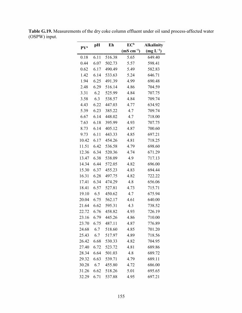
155
Table G.19. Measurements of the dry coke column effluent under oil sand process-affected water
(OSPW) input.
PVa pH Eh ECb Alkalinity
(mS cm−1) (mg L−1)
0.18 6.11 516.38 5.65 649.40
0.44 6.07 502.73 5.57 598.41
0.62 6.17 490.49 5.49 582.83
1.42 6.14 533.63 5.24 646.71
1.94 6.25 491.39 4.99 690.48
2.48 6.29 516.14 4.86 704.59
3.31 6.2 525.99 4.84 707.75
3.58 6.3 538.57 4.84 709.74
4.43 6.22 447.03 4.77 634.92
5.39 6.23 385.22 4.7 709.74
6.67 6.14 448.02 4.7 718.00
7.63 6.18 395.99 4.93 707.75
8.73 6.14 405.12 4.87 700.60
9.73 6.11 443.33 4.85 697.21
10.42 6.17 454.26 4.81 718.25
11.51 6.42 536.58 4.79 698.60
12.36 6.34 520.36 4.74 671.29
13.47 6.38 538.09 4.9 717.13
14.34 6.44 572.05 4.82 696.00
15.30 6.37 455.23 4.83 694.44
16.31 6.28 497.75 4.82 722.22
17.41 6.34 474.29 4.8 656.06
18.41 6.57 527.81 4.73 715.71
19.10 6.5 450.62 4.7 675.94
20.04 6.75 562.17 4.61 640.00
21.64 6.62 595.31 4.3 738.52
22.72 6.76 458.82 4.93 726.19
23.16 6.79 445.26 4.86 710.00
23.70 6.75 487.11 4.87 776.89
24.68 6.7 518.60 4.85 701.20
25.43 6.7 517.97 4.89 718.56
26.42 6.68 530.33 4.82 704.95
27.40 6.72 523.72 4.81 689.86
28.34 6.64 501.03 4.8 689.72
29.32 6.63 539.71 4.79 689.11
30.28 6.7 455.80 4.72 686.00
31.26 6.62 518.26 5.01 695.65
32.29 6.71 537.88 4.95 697.21

156
PVa pH Eh ECb Alkalinity
(mS cm−1) (mg L−1)
33.24 6.73 511.76 4.92 688.62
34.21 6.8 528.94 4.9 664.68
35.06 6.83 496.06 4.83 664.68 aPV: Pore volume
bEC: Electrical conductivity
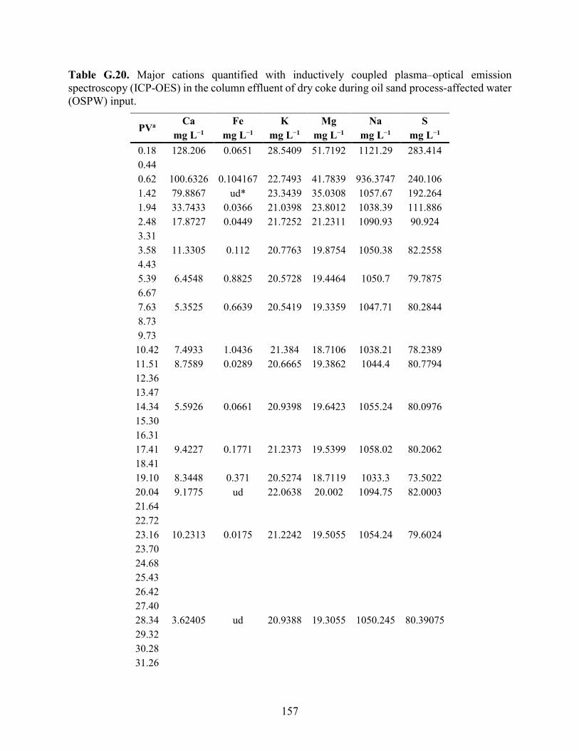
157
Table G.20. Major cations quantified with inductively coupled plasma–optical emission
spectroscopy (ICP-OES) in the column effluent of dry coke during oil sand process-affected water
(OSPW) input.
PVa Ca Fe K Mg Na S
mg L−1 mg L−1 mg L−1 mg L−1 mg L−1 mg L−1
0.18 128.206 0.0651 28.5409 51.7192 1121.29 283.414
0.44
0.62 100.6326 0.104167 22.7493 41.7839 936.3747 240.106
1.42 79.8867 ud* 23.3439 35.0308 1057.67 192.264
1.94 33.7433 0.0366 21.0398 23.8012 1038.39 111.886
2.48 17.8727 0.0449 21.7252 21.2311 1090.93 90.924
3.31
3.58 11.3305 0.112 20.7763 19.8754 1050.38 82.2558
4.43
5.39 6.4548 0.8825 20.5728 19.4464 1050.7 79.7875
6.67
7.63 5.3525 0.6639 20.5419 19.3359 1047.71 80.2844
8.73
9.73
10.42 7.4933 1.0436 21.384 18.7106 1038.21 78.2389
11.51 8.7589 0.0289 20.6665 19.3862 1044.4 80.7794
12.36
13.47
14.34 5.5926 0.0661 20.9398 19.6423 1055.24 80.0976
15.30
16.31
17.41 9.4227 0.1771 21.2373 19.5399 1058.02 80.2062
18.41
19.10 8.3448 0.371 20.5274 18.7119 1033.3 73.5022
20.04 9.1775 ud 22.0638 20.002 1094.75 82.0003
21.64
22.72
23.16 10.2313 0.0175 21.2242 19.5055 1054.24 79.6024
23.70
24.68
25.43
26.42
27.40
28.34 3.62405 ud 20.9388 19.3055 1050.245 80.39075
29.32
30.28
31.26

158
PVa Ca Fe K Mg Na S
mg L−1 mg L−1 mg L−1 mg L−1 mg L−1 mg L−1
32.29
33.24
34.21
35.06 4.4678 ud 21.2054 19.4054 1065.01 79.532 aPV: Pore volume
*ud: concentrations below method detection limit
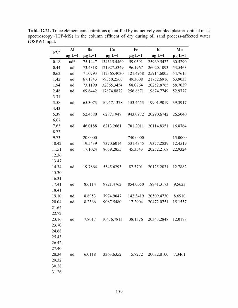
159
Table G.21. Trace element concentrations quantified by inductively coupled plasma–optical mass
spectroscopy (ICP-MS) in the column effluent of dry during oil sand process-affected water
(OSPW) input.
PVa Al Ba Ca Fe K Mo
µg L−1 µg L−1 µg L−1 µg L−1 µg L−1 µg L−1
0.18 ud* 75.1447 134315.4469 59.0391 25969.5422 60.5290
0.44 ud 73.4318 121927.5349 96.1967 26020.1093 53.5463
0.62 ud 71.0793 112365.4030 121.4958 25914.6005 54.7615
1.42 ud 67.1843 79350.2560 49.3608 21752.6916 63.9033
1.94 ud 73.1199 32365.3454 68.0764 20252.8765 58.7039
2.48 ud 69.6442 17874.8872 256.8871 19874.7749 52.9777
3.31
3.58 ud 65.3073 10957.1378 153.4653 19901.9019 39.3917
4.43
5.39 ud 52.4580 6287.1948 943.0972 20290.6742 26.5040
6.67
7.63 ud 46.0188 6213.2661 701.2011 20114.8351 16.8764
8.73
9.73 20.0000 740.0000 15.0000
10.42 ud 19.5439 7370.6014 531.4345 19377.2829 12.4519
11.51 ud 17.1024 8659.2855 45.3543 20252.2168 22.9324
12.36
13.47
14.34 ud 19.7864 5545.6293 87.3701 20125.2031 12.7882
15.30
16.31
17.41 ud 8.6114 9821.4762 854.0050 18941.3173 9.5623
18.41
19.10 ud 8.8953 7974.9047 142.3419 20509.4730 8.6910
20.04 ud 8.2366 9087.5480 17.2904 20472.0751 15.1557
21.64
22.72
23.16 ud 7.8017 10476.7813 38.1376 20343.2848 12.0178
23.70
24.68
25.43
26.42
27.40
28.34 ud 6.0118 3363.6352 15.8272 20032.8100 7.3461
29.32
30.28
31.26
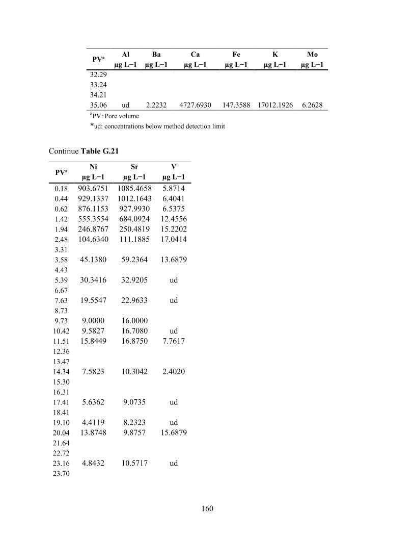
160
PVa Al Ba Ca Fe K Mo
µg L−1 µg L−1 µg L−1 µg L−1 µg L−1 µg L−1
32.29
33.24
34.21
35.06 ud 2.2232 4727.6930 147.3588 17012.1926 6.2628 aPV: Pore volume
*ud: concentrations below method detection limit
Continue Table G.21
PVa Ni Sr V
µg L−1 µg L−1 µg L−1
0.18 903.6751 1085.4658 5.8714
0.44 929.1337 1012.1643 6.4041
0.62 876.1153 927.9930 6.5375
1.42 555.3554 684.0924 12.4556
1.94 246.8767 250.4819 15.2202
2.48 104.6340 111.1885 17.0414
3.31
3.58 45.1380 59.2364 13.6879
4.43
5.39 30.3416 32.9205 ud
6.67
7.63 19.5547 22.9633 ud
8.73
9.73 9.0000 16.0000
10.42 9.5827 16.7080 ud
11.51 15.8449 16.8750 7.7617
12.36
13.47
14.34 7.5823 10.3042 2.4020
15.30
16.31
17.41 5.6362 9.0735 ud
18.41
19.10 4.4119 8.2323 ud
20.04 13.8748 9.8757 15.6879
21.64
22.72
23.16 4.8432 10.5717 ud
23.70

161
PVa Ni Sr V
µg L−1 µg L−1 µg L−1
24.68
25.43
26.42
27.40
28.34 ud 4.8743 5.5401
29.32
30.28
31.26
32.29
33.24
34.21
35.06 ud 4.1365 3.6926 aPV: Pore volume
*ud: concentrations below method detection limit

162
Table G.22. Measurements of the column effluent of slurry coke during oil sand process-affected
water (OSPW) input.
PVa pH Eh ECb Alk
(mS cm−1) (mg L−1)
0.15 6.78 500.63 7.8 1890.00
0.29 6.75 488.50 7.84 1675.25
0.42 6.64 473.33 7.56 1612.33
0.78 6.59 467.32 6.7 1414.34
1.20 6.42 484.99 5.69 1053.68
1.44 6.45 519.99 5.25 908.73
2.24 6.21 468.24 4.89 734.13
3.15 6.17 478.53 4.74 732.67
4.35 6.19 498.72 4.72 731.61
5.25 6.22 461.91 4.94 730.69
6.27 6.2 475.03 4.86 712.57
7.21 6.15 485.72 4.82 700.99
7.73 6.14 505.64 4.78 731.46
8.88 6.3 518.49 4.8 706.00
9.68 6.24 506.25 4.76 706.00
10.71 6.28 527.80 4.89 715.71
11.52 6.27 501.14 4.83 704.00
12.42 6.26 414.85 4.82 717.13
13.37 6.14 468.28 4.81 715.14
14.40 6.27 472.96 4.81 718.56
15.34 6.42 500.23 4.73 691.70
15.99 6.43 453.71 4.67 718.56
16.86 6.61 568.47 4.63 741.48
18.36 6.5 581.02 4.29 718.56
19.37 6.6 430.13 4.92 708.00
19.78 6.68 416.75 4.79 710.00
20.29 6.89 487.61 4.88 775.35
21.20 6.53 511.20 4.85 695.83
21.91 6.4 425.27 4.92 700.00
22.84 6.51 528.03 4.8 712.57
23.75 6.49 531.24 4.8 687.87
24.63 6.42 525.62 4.8 693.23
25.55 6.41 538.31 4.79 691.85
26.46 6.59 498.50 4.71 686.51
27.37 6.52 521.14 5.02 701.20
28.33 6.48 546.76 4.94 685.77
29.22 6.44 515.48 4.91 690.48
30.14 6.61 536.26 4.88 666.67

163
PVa pH Eh ECb Alk
(mS cm−1) (mg L−1)
30.93 6.59 508.88 4.83 670.66 aPV: Pore volume
bEC: Electrical conductivity
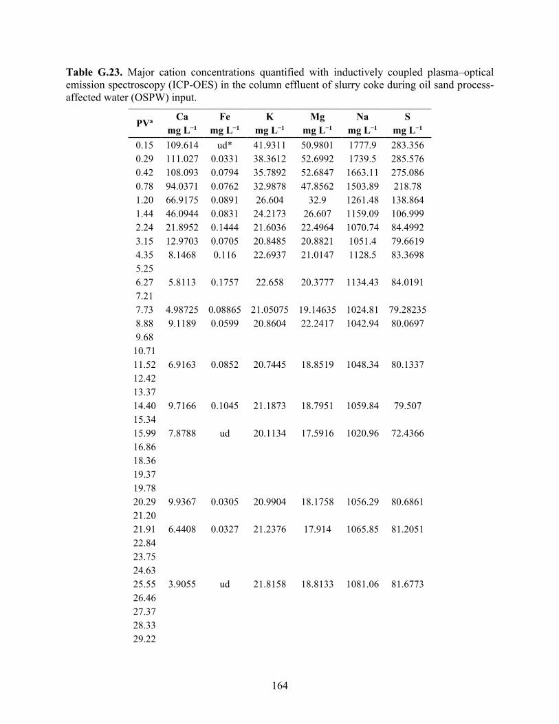
164
Table G.23. Major cation concentrations quantified with inductively coupled plasma–optical
emission spectroscopy (ICP-OES) in the column effluent of slurry coke during oil sand process-
affected water (OSPW) input.
PVa Ca Fe K Mg Na S
mg L−1 mg L−1 mg L−1 mg L−1 mg L−1 mg L−1
0.15 109.614 ud* 41.9311 50.9801 1777.9 283.356
0.29 111.027 0.0331 38.3612 52.6992 1739.5 285.576
0.42 108.093 0.0794 35.7892 52.6847 1663.11 275.086
0.78 94.0371 0.0762 32.9878 47.8562 1503.89 218.78
1.20 66.9175 0.0891 26.604 32.9 1261.48 138.864
1.44 46.0944 0.0831 24.2173 26.607 1159.09 106.999
2.24 21.8952 0.1444 21.6036 22.4964 1070.74 84.4992
3.15 12.9703 0.0705 20.8485 20.8821 1051.4 79.6619
4.35 8.1468 0.116 22.6937 21.0147 1128.5 83.3698
5.25
6.27 5.8113 0.1757 22.658 20.3777 1134.43 84.0191
7.21
7.73 4.98725 0.08865 21.05075 19.14635 1024.81 79.28235
8.88 9.1189 0.0599 20.8604 22.2417 1042.94 80.0697
9.68
10.71
11.52 6.9163 0.0852 20.7445 18.8519 1048.34 80.1337
12.42
13.37
14.40 9.7166 0.1045 21.1873 18.7951 1059.84 79.507
15.34
15.99 7.8788 ud 20.1134 17.5916 1020.96 72.4366
16.86
18.36
19.37
19.78
20.29 9.9367 0.0305 20.9904 18.1758 1056.29 80.6861
21.20
21.91 6.4408 0.0327 21.2376 17.914 1065.85 81.2051
22.84
23.75
24.63
25.55 3.9055 ud 21.8158 18.8133 1081.06 81.6773
26.46
27.37
28.33
29.22

165
PVa Ca Fe K Mg Na S
mg L−1 mg L−1 mg L−1 mg L−1 mg L−1 mg L−1
30.14
30.93 4.8575 ud 22.129 19.0018 1115.06 81.9386 aPV: Pore volume
*ud: concentrations below method detection limit
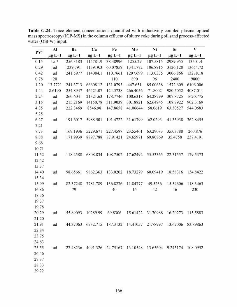
166
Table G.24. Trace element concentrations quantified with inductively coupled plasma–optical
mass spectroscopy (ICP-MS) in the column effluent of slurry coke during oil sand process-affected
water (OSPW) input.
PVa Al Ba Ca Fe Mo Ni Sr V
µg L−1 µg L−1 µg L−1 µg L−1 µg L−1 µg L−1 µg L−1 µg L−1
0.15 Ud* 256.3183 114781.9 38.38996 1255.29 107.5815 2989.955 13501.4
0.29 ud 239.791 113919.3 60.07859 1341.772 106.8915 3126.128 13654.72
0.42 ud 241.5977 114084.1 110.7661 1297.699 113.0335 3006.866 13278.18
0.78 20 110 890 96 2400 9800
1.20 13.7721 241.3713 66608.12 131.0793 447.651 85.00638 1572.609 6106.006
1.44 8.6190 254.8947 46421.07 124.5738 266.4056 71.8002 980.5052 4087.011
2.24 ud 260.6041 21321.63 178.7746 100.6318 64.28799 307.8725 1620.775
3.15 ud 215.2169 14150.78 311.9039 30.18821 62.64945 108.7922 902.3169
4.35 ud 222.3469 8546.98 147.8658 41.06644 58.0619 63.30527 544.0683
5.25
6.27 ud 191.6017 5988.501 191.4722 31.61799 62.0293 41.35938 362.8455
7.21
7.73 ud 169.1936 5229.671 227.4588 23.55461 63.29083 35.03788 260.876
8.88 ud 171.9939 8897.788 87.91421 24.65971 69.80869 35.4758 237.4191
9.68
10.71
11.52 ud 118.2588 6808.834 108.7502 17.62492 55.53365 22.31557 179.5373
12.42
13.37
14.40 ud 98.65661 9862.363 133.0202 18.73279 60.09419 18.58316 134.8422
15.34
15.99 ud 82.37248 7781.789 136.8276 11.84777 49.5236 15.54606 118.3463
16.86 79 40 15 42 16 230
18.36
19.37
19.78
20.29 ud 55.89093 10289.99 69.8306 15.61422 31.70988 16.20273 115.5883
21.20
21.91 ud 44.37063 6732.715 187.3132 14.41057 21.78997 13.62006 83.89863
22.84
23.75
24.63
25.55 ud 27.48236 4091.326 24.75167 13.10548 13.65604 9.245174 108.0952
26.46
27.37
28.33
29.22
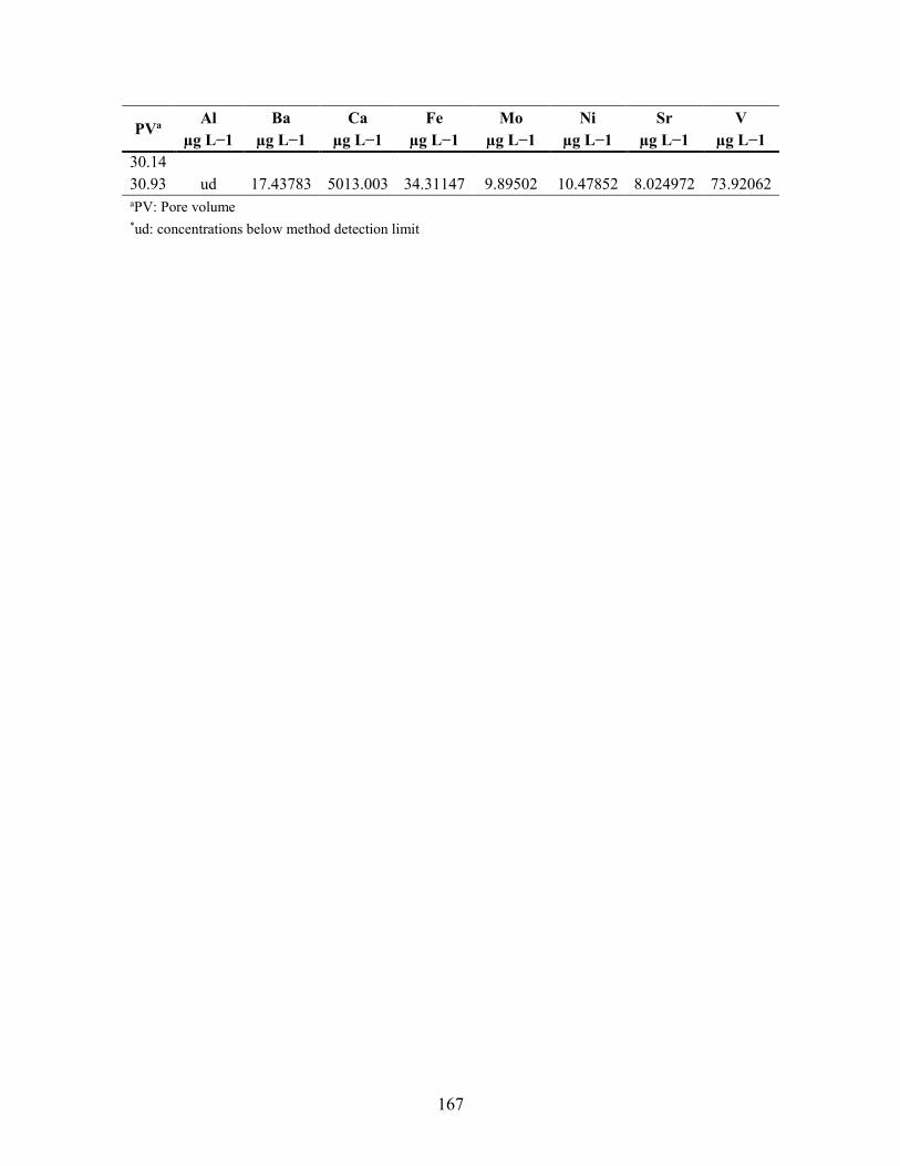
167
PVa Al Ba Ca Fe Mo Ni Sr V
µg L−1 µg L−1 µg L−1 µg L−1 µg L−1 µg L−1 µg L−1 µg L−1
30.14
30.93 ud 17.43783 5013.003 34.31147 9.89502 10.47852 8.024972 73.92062 aPV: Pore volume
*ud: concentrations below method detection limit

168
Table G.25. Measurements of the column influent during acid rock drainage (ARD) input.
PVa pH Eh ECb Alk
(mS cm−1) (mg L−1)
0.24 2.04 838.33 8.38 −
0.39 2.06 840.21 8.39 −
0.54 2 837.37 8.46 −
0.65 2.04 853.22 8.43 −
1.22 2.1 829.31 8.78 −
1.48 2.09 827.80 8.77 −
2.15 2.09 831.58 8.7 −
2.55 2.2 829.24 8.69 −
3.52 2 824.83 8.68 −
3.95 2.12 828.28 8.56 −
5.27 2.05 831.61 8.61 −
6.10 2 836.22 8.5 −
7.19 2.07 827.72 8.76 −
7.92 2.07 827.72 8.76 −
8.03 2.13 829.09 8.65 −
8.98 2.22 825.94 8.69 −
9.96 2.01 825.20 8.9 −
11.04 1.93 836.34 8.84 −
12.02 2.43 829.91 8.76 −
12.68 2.6 834.97 8.63 −
13.61 2.27 830.03 8.53 −
15.18 2.15 830.03 8.53 −
16.24 2.09 836.42 8.4 −
16.67 2.09 836.42 8.4 −
17.20 2.01 843.76 8.56 −
18.02 1.99 833.41 8.79 −
18.95 2 834.65 8.68 −
19.97 2.01 829.41 8.68 −
20.92 2 825.81 8.69 −
21.84 2.08 827.73 8.66 −
22.80 1.94 834.93 8.58 −
23.75 1.98 830.89 8.57 −
24.70 1.9 827.16 8.98 −
25.71 1.97 827.09 8.81 −
26.64 1.93 832.31 8.82 −
27.59 2.04 827.91 8.82 −
28.42 2 830.68 8.66 −
29.47 1.99 824.35 8.81 −
30.41 2.13 827.93 8.78 −

169
PVa pH Eh ECb Alk
(mS cm−1) (mg L−1)
31.05 2.34 827.32 8.55 − aPV: Pore volume
bEC: Electrical conductivity
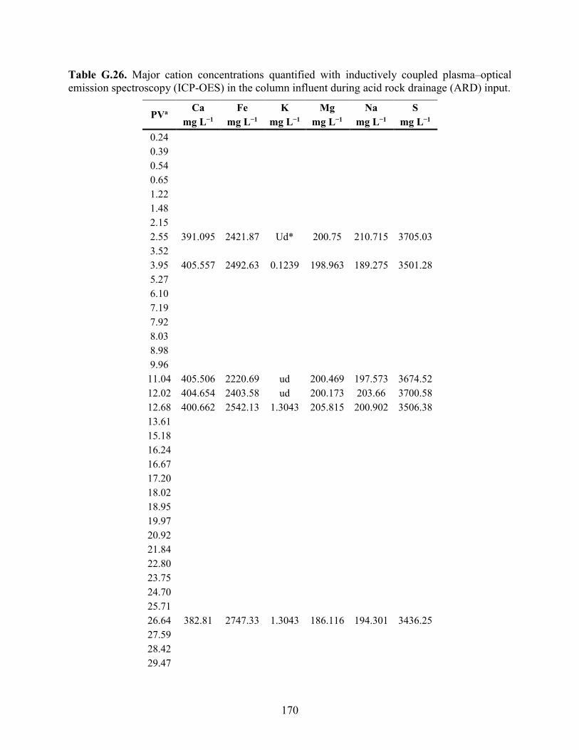
170
Table G.26. Major cation concentrations quantified with inductively coupled plasma–optical
emission spectroscopy (ICP-OES) in the column influent during acid rock drainage (ARD) input.
PVa Ca Fe K Mg Na S
mg L−1 mg L−1 mg L−1 mg L−1 mg L−1 mg L−1
0.24
0.39
0.54
0.65
1.22
1.48
2.15
2.55 391.095 2421.87 Ud* 200.75 210.715 3705.03
3.52
3.95 405.557 2492.63 0.1239 198.963 189.275 3501.28
5.27
6.10
7.19
7.92
8.03
8.98
9.96
11.04 405.506 2220.69 ud 200.469 197.573 3674.52
12.02 404.654 2403.58 ud 200.173 203.66 3700.58
12.68 400.662 2542.13 1.3043 205.815 200.902 3506.38
13.61
15.18
16.24
16.67
17.20
18.02
18.95
19.97
20.92
21.84
22.80
23.75
24.70
25.71
26.64 382.81 2747.33 1.3043 186.116 194.301 3436.25
27.59
28.42
29.47

171
PVa Ca Fe K Mg Na S
mg L−1 mg L−1 mg L−1 mg L−1 mg L−1 mg L−1
30.41
31.05
aPV: Pore volume
*ud: concentrations below method detection limit

172
Table G.27. Trace element concentrations quantified with inductively coupled plasma–optical
mass spectroscopy (ICP-MS) in the columns influent during acid rock drainage (ARD) input.
PVa Al Ba K Mo Ni Sr V
µg L−1 µg L−1 µg L−1 µg L−1 µg L−1 µg L−1 µg L−1
0.24 Ud* 7.2956 185.5526 12.3987 15.4998 98.4764 3.4536
0.39 326.0259 7.5382 193.7886 16.6673 28.9475 110.3974 24.9790
0.54
0.65 ud 7.5071 184.0733 12.3154 14.2887 101.4230 5.0092
1.22
1.48
2.15
2.55
3.52
3.95 20.7077 5.9368 224.1356 ud 13.5609 112.6890 ud
5.27
6.10
7.19
7.92
8.03
8.98
9.96
11.04
12.02
12.68 ud 6.8793 1225.3621 12.8693 15.2498 104.5072 ud
13.61
15.18
16.24
16.67
17.20
18.02
18.95
19.97
20.92
21.84
22.80
23.75
24.70
25.71
26.64 ud 7.3616 ud 11.6360 12.8252 106.6856 3.6375
27.59
28.42
29.47

173
PVa Al Ba K Mo Ni Sr V
µg L−1 µg L−1 µg L−1 µg L−1 µg L−1 µg L−1 µg L−1
30.41
31.05
aPV: Pore volume
*ud: concentrations below method detection limit

174
Table G.28. Measurements of the column effluent for dry coke during acid rock drainage (ARD)
input.
PVa pH Eh ECb Alk
(mS cm−1) (mg L−1)
0.24 2.3 713.22 8.3 −
0.39 2.28 719.54 8.24 −
0.54 2.16 716.13 8.22 −
0.65 2.24 718.22 8.19 −
1.22 2.35 712.99 8.62 −
1.48 2.17 712.00 8.64 −
2.15 2.18 728.59 8.44 −
2.55 2.2 731.33 8.36 −
3.52 2.02 738.04 8.33 −
3.95 2.21 746.44 8.28 −
5.27 2.24 750.92 8.24 −
6.10 2.08 746.46 8.3 −
7.19 2.07 747.19 8.55 −
7.92 2.34 749.29 8.42 −
8.03 2.14 749.28 8.46 −
8.98 2.26 751.34 8.53 −
9.96 2.01 748.58 8.48 −
11.04 1.99 751.71 8.63 −
12.02 2.45 756.50 8.6 −
12.68 2.6 759.89 8.5 −
13.61 2.3 766.27 8.35 −
15.18 2.16 759.02 7.76 −
16.24 1.97 735.74 8.97 −
16.67 1.98 742.86 8.8 −
17.20 2.1 753.06 8.58 −
18.02 2.15 752.21 8.57 −
18.95 1.97 762.45 8.58 −
19.97 2.02 761.32 8.61 −
20.92 2.02 762.91 8.66 −
21.84 2.09 759.81 8.67 −
22.80 1.95 760.41 8.64 −
23.75 1.98 759.71 8.53 −
24.70 1.9 758.03 9.02 −
25.71 1.97 766.05 8.92 −
26.64 1.99 760.56 8.8 −
27.59 2.03 764.93 8.84 −
28.42 2.02 751.78 8.81 −
29.47 2 757.96 8.77 −
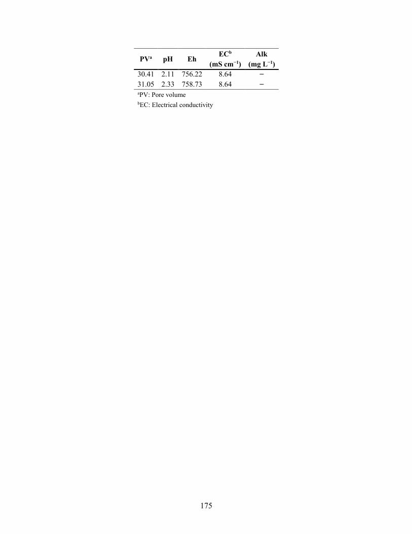
175
PVa pH Eh ECb Alk
(mS cm−1) (mg L−1)
30.41 2.11 756.22 8.64 −
31.05 2.33 758.73 8.64 − aPV: Pore volume
bEC: Electrical conductivity

176
Table G.29. Major cation concentrations quantified with inductively coupled plasma–optical
emission spectroscopy (ICP-OES) in the column effluent form dry coke during acid rock drainage
(ARD) input.
PVa Ca Fe K Mg Na S
mg L−1 mg L−1 mg L−1 mg L−1 mg L−1 mg L−1
0.24 518.6865 2788.56 Ud* 252.871 238.286 3955.77
0.39 521.046 2761.22 ud 240.003 218.953 3826.07
0.54 507.847 2748.51 ud 230.48 211.947 3805.65
0.65 497.087 2510.79 ud 224.533 211.024 3714.41
1.22 458.075 2508.27 ud 216.769 198.918 3831.14
1.48 427.947 2477.92 ud 209.061 209.193 3756.39
2.15
2.55 403.412 2389.33 ud 204.741 211.168 3766.49
3.52
3.95 403.251 2439.355 ud 201.719 191.4585 3574.71
5.27
6.10 398.835 2399.14 ud 203.356 208.811 3728.92
7.19
7.92 397.56 2541.58 ud 201.27 209.594 3733.4
8.03
8.98 405.709 2527.6 ud 197.528 199.456 3646.73
9.96
11.04
12.02
12.68 401.7285 2429.805 ud 205.8725 195.996 3456.845
13.61
15.18
16.24
16.67
17.20 402.92 2156.97 ud 196.082 381.778 3312.55
18.02
18.95
19.97 403.583 2637.38 ud 195.934 190.751 3629.44
20.92
21.84
22.80
23.75
24.70
25.71
26.64 400.12 2674.44 ud 194.864 184.561 3378.41
27.59
28.42

177
PVa Ca Fe K Mg Na S
mg L−1 mg L−1 mg L−1 mg L−1 mg L−1 mg L−1
29.47
30.41
31.05 399.722 2616.21 ud 197.517 195.382 3658.94 aPV: Pore volume
*ud: concentrations below method detection limit
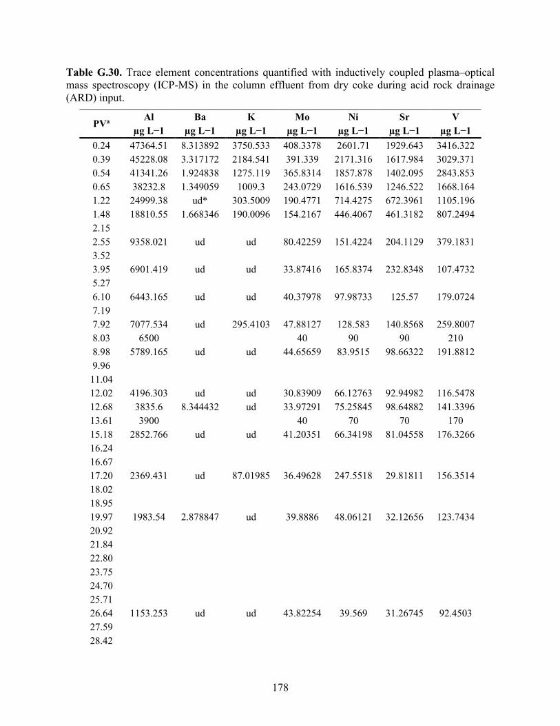
178
Table G.30. Trace element concentrations quantified with inductively coupled plasma–optical
mass spectroscopy (ICP-MS) in the column effluent from dry coke during acid rock drainage
(ARD) input.
PVa Al Ba K Mo Ni Sr V
µg L−1 µg L−1 µg L−1 µg L−1 µg L−1 µg L−1 µg L−1
0.24 47364.51 8.313892 3750.533 408.3378 2601.71 1929.643 3416.322
0.39 45228.08 3.317172 2184.541 391.339 2171.316 1617.984 3029.371
0.54 41341.26 1.924838 1275.119 365.8314 1857.878 1402.095 2843.853
0.65 38232.8 1.349059 1009.3 243.0729 1616.539 1246.522 1668.164
1.22 24999.38 ud* 303.5009 190.4771 714.4275 672.3961 1105.196
1.48 18810.55 1.668346 190.0096 154.2167 446.4067 461.3182 807.2494
2.15
2.55 9358.021 ud ud 80.42259 151.4224 204.1129 379.1831
3.52
3.95 6901.419 ud ud 33.87416 165.8374 232.8348 107.4732
5.27
6.10 6443.165 ud ud 40.37978 97.98733 125.57 179.0724
7.19
7.92 7077.534 ud 295.4103 47.88127 128.583 140.8568 259.8007
8.03 6500 40 90 90 210
8.98 5789.165 ud ud 44.65659 83.9515 98.66322 191.8812
9.96
11.04
12.02 4196.303 ud ud 30.83909 66.12763 92.94982 116.5478
12.68 3835.6 8.344432 ud 33.97291 75.25845 98.64882 141.3396
13.61 3900 40 70 70 170
15.18 2852.766 ud ud 41.20351 66.34198 81.04558 176.3266
16.24
16.67
17.20 2369.431 ud 87.01985 36.49628 247.5518 29.81811 156.3514
18.02
18.95
19.97 1983.54 2.878847 ud 39.8886 48.06121 32.12656 123.7434
20.92
21.84
22.80
23.75
24.70
25.71
26.64 1153.253 ud ud 43.82254 39.569 31.26745 92.4503
27.59
28.42
179
PVa Al Ba K Mo Ni Sr V
µg L−1 µg L−1 µg L−1 µg L−1 µg L−1 µg L−1 µg L−1
29.47
30.41
31.05 669.2527 ud ud 21.32908 25.09269 18.21648 56.44334 aPV: Pore volume
*ud: concentrations below method detection limit

180
Table G.31. Measurements of the column effluent from slurry coke during acid rock drainage
(ARD) input.
PVa pH Eh ECb Alk
(mS cm−1) (mg L−1)
0.20 3.31 553.93 11.98 −
0.32 3.15 579.35 11.62 −
0.46 2.86 622.34 10.72 −
0.61 2.65 650.65 9.89 −
0.74 2.67 666.06 9.07 −
0.85 2.41 669.45 8.86 −
1.79 2.38 695.03 8.63 −
2.77 2.11 700.83 8.56 −
3.85 2.01 705.78 8.7 −
4.82 2.49 710.31 8.67 −
5.47 2.59 706.53 8.6 −
6.40 2.3 712.44 8.57 −
7.96 2.22 712.90 7.97 −
9.00 2.01 698.44 9.4 −
9.43 1.93 698.96 9.23 −
9.55 1.93 698.31 9.18 −
9.96 2.09 700.70 9 −
10.77 2.12 699.59 9.01 −
11.70 1.91 709.39 9.05 −
12.71 2.03 708.52 8.97 −
13.66 2.01 713.24 8.92 −
14.57 2.07 708.83 9 −
15.53 1.94 712.21 8.98 −
16.46 1.98 716.50 8.85 −
17.41 1.9 712.36 9.27 −
18.41 1.97 717.96 9.19 −
19.33 1.92 714.14 9.1 −
20.29 2.04 718.16 9.02 −
21.11 2.03 715.38 8.92 −
22.15 1.98 717.78 8.84 −
23.09 2.11 718.22 8.46 −
23.72 2.32 718.41 8.8 −
24.72 1.99 723.20 8.77 −
25.40 2 721.89 9.22 −
26.00 2.07 721.32 9.22 −
26.44 2.01 717.46 9.32 −
27.26 2.05 715.84 9.22 −
27.68 2.03 716.74 9.2 −

181
PVa pH Eh ECb Alk
(mS cm−1) (mg L−1)
27.95 2 717.83 9.23 −
28.04 2.06 721.83 9.12 −
29.12 2.01 722.72 9.07 −
29.38 2.01 721.52 9.17 −
30.52 2 720.34 9.14 −
31.02 2 720.56 9.12 − aPV: Pore volume
bEC: Electrical conductivity

182
Table G.32. Major cation concentrations quantified with inductively coupled plasma–optical
emission spectroscopy (ICP-OES) in the column effluent from slurry coke during acid rock
drainage (ARD) input.
PVa Al Ca Fe K Mg Na S
mg L−1 mg L−1 mg L−1 mg L−1 mg L−1 mg L−1 mg L−1
0.20 212.2635 501.4355 1672.9 59.7396 366.9345 1582.435 3829.145
0.32 215.886 501.093 1713.18 53.3541 355.381 1418.96 3795.44
0.46 197.823 499.718 1930.62 31.3023 331.531 1062.11 3809.08
0.61 167.311 500.505 2146.32 19.1728 291.32 761.107 3820.63
0.74 103.844 520.728 2341 8.2119 238.562 419.508 3646.72
0.85
1.79 26.4966 492.92 2458.33 Ud* 201.451 196.758 3695.12
2.77 16.6781 420.921 2308.53 ud 200.682 196.247 3621.2
3.85 10.4263 409.854 2289.43 ud 198.701 193.978 3675.25
4.82
5.47 6.5058 405.293 2462.96 ud 204.329 190.51 3437.78
6.40 5.9008 408.438 2712.19 ud 203.654 199.538 3801.74
7.96 4.1204 403.259 2660.6 ud 196.546 190.363 3646.55
9.00
9.43
9.55
9.96 3.48795 407.038 2060.37 ud 197.2355 392.954 3288.55
10.77
11.70
12.71 2.4172 406.877 2622.36 ud 194.402 182.189 3636.57
13.66
14.57
15.53
16.46
17.41
18.41
19.33 0.5881 383.8765 2688.355 ud 187.307 178.4755 3355.075
20.29
21.11
22.15
23.09
23.72
24.72 1.1757 402.713 2614.17 ud 207.734 200.211 3793.34
25.40
26.00
26.44
27.26 1.646 405.785 2590.54 ud 205.756 193.073 3728.08

183
PVa Al Ca Fe K Mg Na S
mg L−1 mg L−1 mg L−1 mg L−1 mg L−1 mg L−1 mg L−1
27.68
27.95
28.04
29.12
29.38 0.9521 407.305 2588.82 ud 207.709 195.28 3808.73
30.52
31.02 0.8078 393.059 2621.68 ud 197.802 180.581 3220.31 aPV: Pore volume
*ud: concentrations below method detection limit
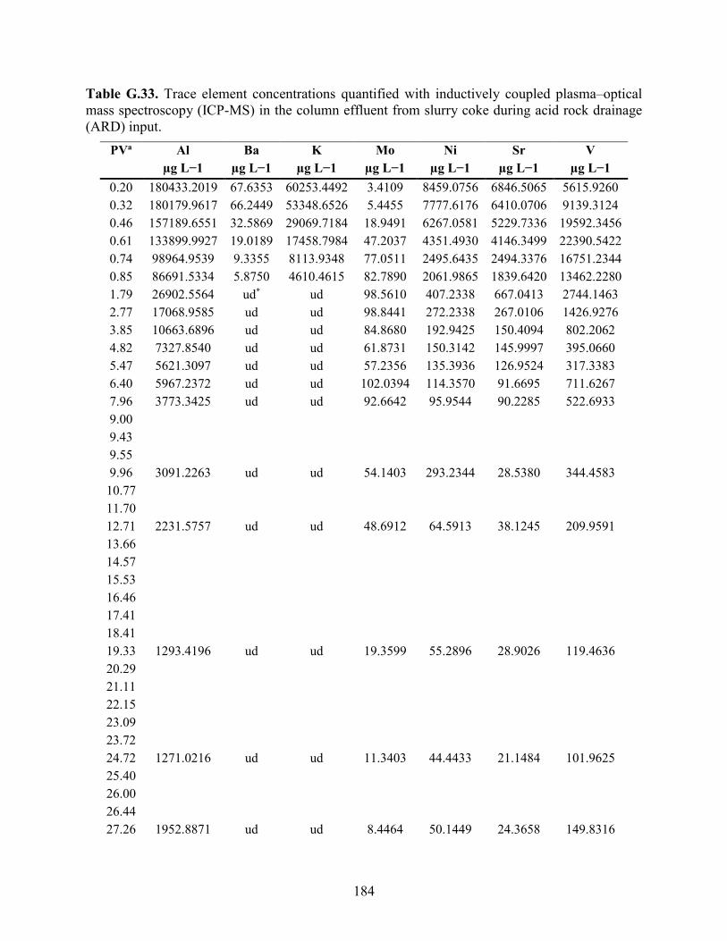
184
Table G.33. Trace element concentrations quantified with inductively coupled plasma–optical
mass spectroscopy (ICP-MS) in the column effluent from slurry coke during acid rock drainage
(ARD) input.
PVa Al Ba K Mo Ni Sr V
µg L−1 µg L−1 µg L−1 µg L−1 µg L−1 µg L−1 µg L−1
0.20 180433.2019 67.6353 60253.4492 3.4109 8459.0756 6846.5065 5615.9260
0.32 180179.9617 66.2449 53348.6526 5.4455 7777.6176 6410.0706 9139.3124
0.46 157189.6551 32.5869 29069.7184 18.9491 6267.0581 5229.7336 19592.3456
0.61 133899.9927 19.0189 17458.7984 47.2037 4351.4930 4146.3499 22390.5422
0.74 98964.9539 9.3355 8113.9348 77.0511 2495.6435 2494.3376 16751.2344
0.85 86691.5334 5.8750 4610.4615 82.7890 2061.9865 1839.6420 13462.2280
1.79 26902.5564 ud* ud 98.5610 407.2338 667.0413 2744.1463
2.77 17068.9585 ud ud 98.8441 272.2338 267.0106 1426.9276
3.85 10663.6896 ud ud 84.8680 192.9425 150.4094 802.2062
4.82 7327.8540 ud ud 61.8731 150.3142 145.9997 395.0660
5.47 5621.3097 ud ud 57.2356 135.3936 126.9524 317.3383
6.40 5967.2372 ud ud 102.0394 114.3570 91.6695 711.6267
7.96 3773.3425 ud ud 92.6642 95.9544 90.2285 522.6933
9.00
9.43
9.55
9.96 3091.2263 ud ud 54.1403 293.2344 28.5380 344.4583
10.77
11.70
12.71 2231.5757 ud ud 48.6912 64.5913 38.1245 209.9591
13.66
14.57
15.53
16.46
17.41
18.41
19.33 1293.4196 ud ud 19.3599 55.2896 28.9026 119.4636
20.29
21.11
22.15
23.09
23.72
24.72 1271.0216 ud ud 11.3403 44.4433 21.1484 101.9625
25.40
26.00
26.44
27.26 1952.8871 ud ud 8.4464 50.1449 24.3658 149.8316

185
PVa Al Ba K Mo Ni Sr V
µg L−1 µg L−1 µg L−1 µg L−1 µg L−1 µg L−1 µg L−1
27.68
27.95
28.04
29.12
29.38 1222.5877 ud ud 11.4600 45.1734 21.1013 83.8479
30.52
31.02 1220.0344 ud ud 7.4563 38.5321 15.8389 65.8891
aPV: Pore volume
*ud: concentrations below method detection limit

186
APPENDIX H: CUMULATIVE MASS RELEASE
Table H.1. Cumulative mass release per kg of fluid petroleum coke for the small columns. DC:
dry coke; SC: slurry coke.
Elements DIa (µg kg−1) OSPWb (µg kg−1) ARDc (µg kg−1)
DC SC DC SC DC SC
V 1.27 5030 70.5 10100 3290 12800
Ni 1170 1330 760 651 2110 3550
Mo 3.82 514 276 869 758 610
Al 4500 6980 0.00 7.94 80000 127000
Mn 3540 2690 3030 1570 6550 5310
Ti 0.00 5.56 1.60 35.9 605 1220
Sr 1060 2810 890 2030 1820 2820
Se 0.31 177 2.00 326 399 1050
Co 145.0 102 99.8 46.3 404 387
As 1.61 6.28 0.00 8.53 73 155
U 0.00 1.06 0.08 2.44 6.33 14
Zn 14500 8300 4610 2270 29900 28600
Cu 11.8 15.6 911 2320 581 425
aDI: Deionized water
bOSPW: synthetic oil sand processing affected water
cARD: Acid rock drianage

187
Table H.2. Cumulative mass release during sequential water input phases for the large column.
Negative values mean attenuation in their concentrations.
Elements DIa
(µg kg−1)
OSPWb
(µg kg−1)
OSPWc
(µg kg−1)
ARDd
(µg kg−1)
Total
(µg kg−1) Leaching efficiency
V 13 123 49 4160 4350 0.31%
Ni 803 0 -10 1360 2160 0.40%
Mo 4 280 2 235 520 0.69%
Al 3540 6 354 63500 67400 0.94
Mn 2980 156 3 2970 6100 7.89
Ti 1 2 2 479 483 0.03
Sr 860 54 -130 380 1170 1.47
Se 20 1 -16 290 295 29.46
Co 92 1 2 204 298 4.81
As 0 0 -31 45 14 0.62
U 0 0 -22 21 -1 0
Zn 3430 50 14 750 4240 12.34
Cu 240 80 -58 600 850 7.36 aDI: Deionized water
bOSPW: synthetic oil sand processing affected water cOSPW: field oil sand processing affected water
dARD: Acid rock drainage

188
APPENDIX I: BREAKTHROUGH CURVE
Figure I.1. Breakthrough curve for the first tracer test of the large column; injection (top) and
decay (bottom). Error bars represent the electrode ±2.5% electrode sensitivity. Red dashed lines
indicate the lower and higher 95% confidence.

189
Figure I.2. Breakthrough curve for the decay part of the second tracer test on the large column.
Error bars represent the electrode ±2.5% electrode sensitivity. Red dashed lines indicate the lower
and higher 95% confidence.


