Download - Mechanism kinematics & dynamics.pdf

8/11/2019 Mechanism kinematics & dynamics.pdf
http://slidepdf.com/reader/full/mechanism-kinematics-dynamicspdf 1/269
Mechanism Kinematics & Dynamics and
Vibrational Modeling
Dr. Robert L. Williams IIMechanical Engineering, Ohio University
NotesBook Supplement forME 3011 Kinematics & Dynamics of Machines
© 2014 Dr. Bob Productions
[email protected] people.ohio.edu/williar4
These notes supplement the ME 3011 NotesBook by Dr. Bob
This document presents supplemental notes to accompany the ME 3011 NotesBook. The outlinegiven in the Table of Contents on the next page dovetails with and augments the ME 3011 NotesBook
outline and hence is incomplete here.
mk
x(t)
k
x (t) x (t)
8/11/2019 Mechanism kinematics & dynamics.pdf
http://slidepdf.com/reader/full/mechanism-kinematics-dynamicspdf 2/269
2
ME 3011 Supplement Table of Contents
1. INTRODUCTION................................................................................................................................ 4
1.3 VECTORS. CARTESIAN R E-IM R EPRESENTATION (PHASORS) ............................................................. 41.6 MATRICES .......................................................................................................................................... 6
2. KINEMATICS ANALYSIS .............................................................................................................. 15
2.1 POSITION K INEMATICS A NALYSIS .................................................................................................... 152.1.1 Four-Bar Mechanism Position Analysis .................................................................................. 15
2.1.1.1 Tangent Half-Angle Substitution Derivation and Alternate Solution Method .................. 152.1.1.3 Four-Bar Mechanism Solution Irregularities ..................................................................... 202.1.1.4 Grashof’s Law and Four-Bar Mechanism Joint Limits ..................................................... 21
2.1.2 Slider-Crank Mechanism Position Analysis ............................................................................. 29 2.1.3 Inverted Slider-Crank Mechanism Position Analysis .............................................................. 32 2.1.4 Multi-Loop Mechanism Position Analysis ............................................................................... 38
2.2 VELOCITY K INEMATICS A NALYSIS .................................................................................................. 422.2.2 Three-Part Velocity Formula Moving Example ....................................................................... 42 2.2.3 Four-Bar Mechanism Velocity Analysis .................................................................................. 44 2.2.5 Inverted Slider-Crank Mechanism Velocity Analysis............................................................... 45 2.2.6 Multi-Loop Mechanism Velocity Analysis ................................................................................ 49
2.3 ACCELERATION K INEMATICS A NALYSIS .......................................................................................... 532.3.2 Five-Part Acceleration Formula Moving Example .................................................................. 53 2.3.3 Four-Bar Mechanism Acceleration Analysis ........................................................................... 55 2.3.4 Slider-Crank Mechanism Acceleration Analysis ...................................................................... 56 2.3.5 Inverted Slider-Crank Mechanism Acceleration Analysis ....................................................... 57 2.3.6 Multi-Loop Mechanism Acceleration Analysis ........................................................................ 63
2.4 OTHER K INEMATICS TOPICS ............................................................................................................ 672.4.1 Link Extensions Graphics ......................................................................................................... 67
2.5 JERK K INEMATICS A NALYSIS ........................................................................................................... 692.5.1 Jerk Analysis Introduction ....................................................................................................... 69 2.5.2 Mechanism Jerk Analysis ......................................................................................................... 72
2.6 BRANCH SYMMETRY IN K INEMATICS A NALYSIS .............................................................................. 732.6.1 Four-Bar Mechanism ............................................................................................................... 73 2.6.2 Slider-Crank Mechanism.......................................................................................................... 75
2.7 K INEMATICS A NALYSIS EXAMPLES ................................................................................................. 772.7.1 Term Example 1: Four-Bar Mechanism .................................................................................. 77 2.7.2 Term Example 2: Slider-Crank Mechanism ............................................................................. 88
3. DYNAMICS ANALYSIS .................................................................................................................. 95
3.1 DYNAMICS I NTRODUCTION .............................................................................................................. 953.2 MASS, CENTER OF GRAVITY, AND MASS MOMENT OF I NERTIA ....................................................... 963.4 FOUR -BAR MECHANISM I NVERSE DYNAMICS A NALYSIS ............................................................... 1083.5 SLIDER -CRANK MECHANISM I NVERSE DYNAMICS A NALYSIS ....................................................... 1113.6 I NVERTED SLIDER -CRANK MECHANISM I NVERSE DYNAMICS A NALYSIS....................................... 1133.7 MULTI-LOOP MECHANISM I NVERSE DYNAMICS A NALYSIS ............................................................ 1213.8 BALANCING OF R OTATING SHAFTS ................................................................................................ 1263.9 I NVERSE DYNAMICS A NALYSIS EXAMPLES .................................................................................... 130
3.9.1 Single Rotating Link Inverse Dynamics Example .................................................................. 130
8/11/2019 Mechanism kinematics & dynamics.pdf
http://slidepdf.com/reader/full/mechanism-kinematics-dynamicspdf 3/269
3
3.9.2 Term Example 1: Four-Bar Mechanism ................................................................................ 133 3.9.3 Term Example 2: Slider-Crank Mechanism ........................................................................... 139
4. GEARS AND CAMS ....................................................................................................................... 145
4.1 GEARS ............................................................................................................................................ 1454.1.1 Gear Introduction ................................................................................................................... 145 4.1.2 Gear Ratio .............................................................................................................................. 151
4.1.3 Gear Trains ............................................................................................................................ 154 4.1.4 Involute Spur Gear Standardization ...................................................................................... 156 4.1.5 Planetary Gear Trains ........................................................................................................... 165
4.2 CAMS ............................................................................................................................................. 1734.2.1 Cam Introduction ................................................................................................................... 173 4.2.2 Cam Motion Profiles .............................................................................................................. 176 4.2.3 Analytical Cam Synthesis ....................................................................................................... 181
5. MECHANICAL VIBRATIONS INTRODUCTION .................................................................... 188
5.2 MECHANICAL VIBRATIONS DEFINITIONS ....................................................................................... 188
6. VIBRATIONAL SYSTEMS MODELING.................................................................................... 191
6.1 ZEROTH-ORDER SYSTEMS ............................................................................................................. 1916.2 SECOND-ORDER SYSTEMS ............................................................................................................. 201
6.2.1 Translational m-c-k System Dynamics Model ........................................................................ 201 6.2.3 Pendulum System Dynamics Model ....................................................................................... 202 6.2.4 Uniform Circular Motion ....................................................................................................... 204
6.4 ADDITIONAL 1-DOF VIBRATIONAL SYSTEMS MODELS ................................................................... 2056.5 ELECTRICAL CIRCUITS MODELING ................................................................................................. 2376.6 MULTI-DOF VIBRATIONAL SYSTEMS MODELS ............................................................................... 246

8/11/2019 Mechanism kinematics & dynamics.pdf
http://slidepdf.com/reader/full/mechanism-kinematics-dynamicspdf 4/269
4
1. Introduction
1.3 Vectors . Cartesian Re-Im Representation (Phasors)
Here is an alternate vector representation.
iP Pe
The phasor iPe
is a polar representation for vectors, where P is the length of vector P , e is the
natural logarithm base, 1i is the imaginary operator, and is the angle of vector P . ie
gives the
direction of the length P, according to Euler’s identity.
cos sinie i
ie
is a unit vector in the direction of vector P .
Phasor Re- Im representation of a vector is equivalent to Cartesian XY representation, where the real ( Re)
axis is along X (or i ) and the imaginary ( Im) axis is along Y (or j ).
cos(cos sin )
sin
cosˆ ˆ(cos sin )
sin
Re i
Im
X
Y
P PP P i Pe
P P
P PP P i j
P P
A strength of Cartesian Re- Im representation using phasors is in taking time derivatives of vectors – the
derivative of the exponential is easy ( ( )s sd ds e e ).2 2
2 2
2
2
22 2
2
22
2
22
2
( )
2
cos 2 sin sin cos
sin 2 cos cos
i
i i
i i i i i
i i i i
d P d Pe
dt dt
d P d Pe iP e
dt dt
d PPe iP e iP e iP e i P edt
d PPe iP e iP e P e
dt
P P P Pd P
dt P P P
2sinP
8/11/2019 Mechanism kinematics & dynamics.pdf
http://slidepdf.com/reader/full/mechanism-kinematics-dynamicspdf 5/269
5
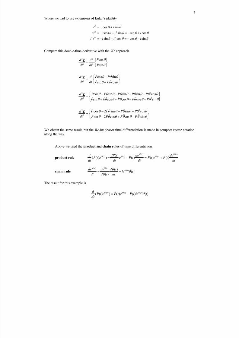
Where we had to use extensions of Euler’s identity
2
2 2
cos sin
cos sin sin cos
sin cos cos sin
i
i
i
e i
ie i i i
i e i i i
Compare this double-time-derivative with the XY approach.
2 2
2 2
2
2
22
2 2
2
2
cos
sin
cos sin
sin cos
cos sin sin sin cos
sin cos cos cos sin
cos 2 sin
Pd P d
Pdt dt
P Pd P d
dt dt P P
P P P P Pd P
dt P P P P P
P P Pd P
dt
2
2
sin cos
sin 2 cos cos sin
P
P P P P
We obtain the same result, but the Re- Im phasor time differentiation is made in compact vector notationalong the way.
Above we used the product and chain rules of time differentiation.
product rule ( ) ( )
( ) ( ) ( )( )( ( ) ) ( ) ( ) ( )
i t i t i t i t i t d dP t de de
P t e e P t P t e P t dt dt dt dt
chain rule ( ) ( )
( )( )( )
( )
i t i t i t de de d t
ie t dt d t dt
The result for this example is
( ) ( ) ( )( ( ) ) ( ) ( ) ( )i t i t i t d P t e P t e P t ie t
dt

8/11/2019 Mechanism kinematics & dynamics.pdf
http://slidepdf.com/reader/full/mechanism-kinematics-dynamicspdf 6/269
6
1.6 Matrices
Matrix an m x n array of numbers, where m is the number of rows and n is the number of columns.
11 12 1
21 22 2
1 2
n
n
m m mn
a a a
a a a A
a a a
Matrices may be used to simplify and standardize the solution of n linear equations in n unknowns(where m = n). Matrices are used in velocity, acceleration, and dynamics linear equations (matrices arenot used in position analysis which requires a non-linear solution).
Special Matrices
square matrix (m = n = 3) 11 12 13
21 22 23
31 32 33
a a a
A a a a
a a a
diagonal matrix 11
22
33
0 0
0 0
0 0
a
A a
a
identity matrix 3
1 0 0
0 1 0
0 0 1
I
transpose matrix 11 21 31
12 22 32
13 23 33
T
a a a
A a a a
a a a
(switch rows & columns)
symmetric matrix 11 12 13
12 22 23
13 23 33
T
a a a
A A a a a
a a a
column vector (3x1 matrix) 1
2
3
x
X x
x
row vector (1x3 matrix) 1 2 3
T X x x x
8/11/2019 Mechanism kinematics & dynamics.pdf
http://slidepdf.com/reader/full/mechanism-kinematics-dynamicspdf 7/269
7
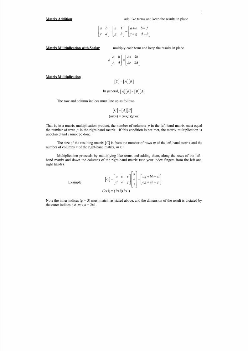
Matrix Addition add like terms and keep the results in place
a b e f a e b f
c d g h c g d h
Matrix Multiplication with Scalar multiply each term and keep the results in place
a b ka kbk
c d kc kd
Matrix Multiplication
C A B
In general, A B B A
The row and column indices must line up as follows.
( x ) ( x )( x )
C A B
m n m p p n
That is, in a matrix multiplication product, the number of columns p in the left-hand matrix must equalthe number of rows p in the right-hand matrix. If this condition is not met, the matrix multiplication isundefined and cannot be done.
The size of the resulting matrix [C ] is from the number of rows m of the left-hand matrix and thenumber of columns n of the right-hand matrix, m x n.
Multiplication proceeds by multiplying like terms and adding them, along the rows of the left-hand matrix and down the columns of the right-hand matrix (use your index fingers from the left andright hands).
Example
(2x1) (2x3)(3x1)
ga b c ag bh ci
C hd e f dg eh fi
i
Note the inner indices ( p = 3) must match, as stated above, and the dimension of the result is dictated bythe outer indices, i.e. m x n = 2x1.

8/11/2019 Mechanism kinematics & dynamics.pdf
http://slidepdf.com/reader/full/mechanism-kinematics-dynamicspdf 8/269
8
Matrix Multiplication Examples
1 2 3
4 5 6 A
7 8
9 8
7 6
B
7 8
1 2 39 8
4 5 67 6
7 18 21 8 16 18 46 42
28 45 42 32 40 36 115 108
C A B
(2x2) (2x3)(3x2)
7 81 2 3
9 84 5 6
7 6
7 32 14 40 21 48 39 54 69
9 32 18 40 27 48 41 58 75
7 24 14 30 21 36 31 44 57
D B A
(3x3) (3x2)(2x3)

8/11/2019 Mechanism kinematics & dynamics.pdf
http://slidepdf.com/reader/full/mechanism-kinematics-dynamicspdf 9/269
9
Matrix Inversion
Since we cannot divide by a matrix, we multiply by the matrix inverse instead. Given
C A B , solve for [ B].
C A B
1 1 A C A A B
I B
B
1
B A C
Matrix [ A] must be square (m = n) to invert.
1 1
A A A A I
where [ I ] is the identity matrix, the matrix 1 (ones on the diagonal and zeros everywhere else). Tocalculate the matrix inverse use the following expression.
1 adjoint( ) A
A A
where A is the determinant of [ A].
adjoint( ) cofactor( ) T
A A
cofactor( A) ( 1)i j
ij ija M
minor minor M ij is the determinant of the submatrix with row i andcolumn j removed.
For another example, given C A B , solve for [ A]
C A B
1 1C B A B B
A I
A
1
A C B
In general the order of matrix multiplication and inversion is crucial and cannot be changed.
8/11/2019 Mechanism kinematics & dynamics.pdf
http://slidepdf.com/reader/full/mechanism-kinematics-dynamicspdf 10/269
10
Matrix Determinant The determinant of a square n x n matrix is a scalar. The matrix determinant is undefined for a
non-square matrix. The determinant of a square matrix A is denoted det( A) or A . The determinant
notation should not be confused with the absolute-value symbol. The MATLAB function for matrixdeterminant is det(A).
If a nonhomogeneous system of n linear equations in n unknowns is dependent, the coefficientmatrix A is singular, and the determinant of matrix A is zero. In this case no unique solution exists tothese equations. On the other hand, if the matrix determinant is non-zero, then the matrix is non-singular, the system of equations is independent, and a unique solution exists.
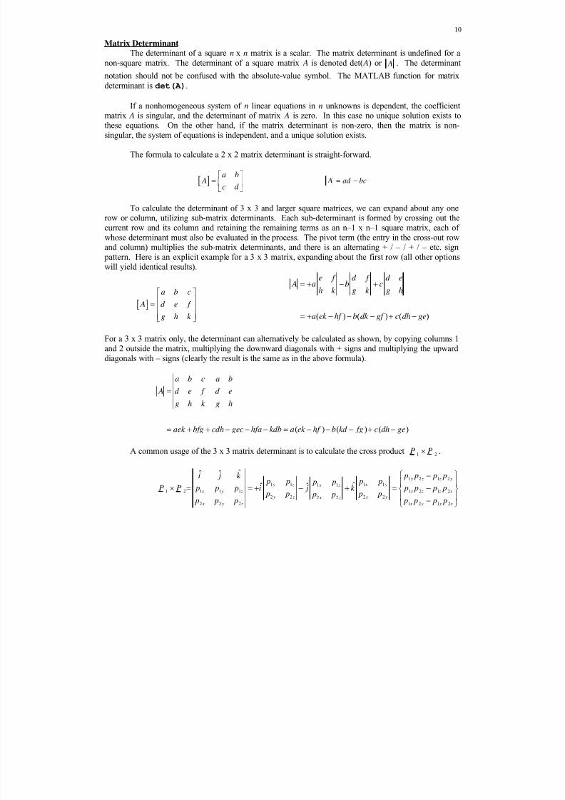
The formula to calculate a 2 x 2 matrix determinant is straight-forward.
a b
Ac d
A ad bc
To calculate the determinant of 3 x 3 and larger square matrices, we can expand about any one
row or column, utilizing sub-matrix determinants. Each sub-determinant is formed by crossing out thecurrent row and its column and retaining the remaining terms as an n–1 x n–1 square matrix, each ofwhose determinant must also be evaluated in the process. The pivot term (the entry in the cross-out rowand column) multiplies the sub-matrix determinants, and there is an alternating + / – / + / – etc. sign pattern. Here is an explicit example for a 3 x 3 matrix, expanding about the first row (all other optionswill yield identical results).
a b c
A d e f
g h k
( ) ( ) ( )
e f d f d e A a b c
h k g k g h
a ek hf b dk gf c dh ge
For a 3 x 3 matrix only, the determinant can alternatively be calculated as shown, by copying columns 1and 2 outside the matrix, multiplying the downward diagonals with + signs and multiplying the upwarddiagonals with – signs (clearly the result is the same as in the above formula).
( ) ( ) ( )
a b c a b
A d e f d e
g h k g h
aek bfg cdh gec hfa kdb a ek hf b kd fg c dh ge
A common usage of the 3 x 3 matrix determinant is to calculate the cross product 1 2P P .
1 2 1 2
1 1 1 11 1
1 2 1 1 1 1 2 1 2
2 2 2 22 2
2 2 2 1 2 1 2
ˆˆ ˆ
ˆˆ ˆ y z z y
y z x y x z
x y z x z z x
y z x y x z
x y z x y y x
i j k p p p p p p p p p p
P P p p p i j k p p p p p p p p p p
p p p p p p p

8/11/2019 Mechanism kinematics & dynamics.pdf
http://slidepdf.com/reader/full/mechanism-kinematics-dynamicspdf 11/269
11
System of Linear Equations
We can solve n linear equations in n unknowns with the help of a matrix. Below is an examplefor n = 3.
11 1 12 2 13 3 1
21 1 22 2 23 3 2
31 1 32 2 33 3 3
a x a x a x b
a x a x a x ba x a x a x b
Where aij are the nine known numerical equation coefficients, xi are the three unknowns, and bi are thethree known right-hand-side terms. Using matrix multiplication backwards, this is written as
A x b .
11 12 13 1 1
21 22 23 2 2
31 32 33 3 3
a a a x b
a a a x b
a a a x b
where
11 12 13
21 22 23
31 32 33
a a a
A a a a
a a a
is the matrix of known numerical coefficients
1
2
3
x x x
x
is the vector of unknowns to be solved and
1
2
3
b
b b
b
is the vector of known numerical right-hand-side terms.
There is a unique solution 1
x A b
only if [ A] has full rank. If not, 0 A (the determinant ofcoefficient matrix [ A] is zero) and the inverse of matrix [ A] is undefined (since it would require dividing by zero; in this case the rank is not full, it is less than 3, which means not all rows/columns of [ A] arelinearly independent). Gaussian Elimination is more robust and more computationally efficient thanmatrix inversion to solve the problem A x b for { x}.
8/11/2019 Mechanism kinematics & dynamics.pdf
http://slidepdf.com/reader/full/mechanism-kinematics-dynamicspdf 12/269
12
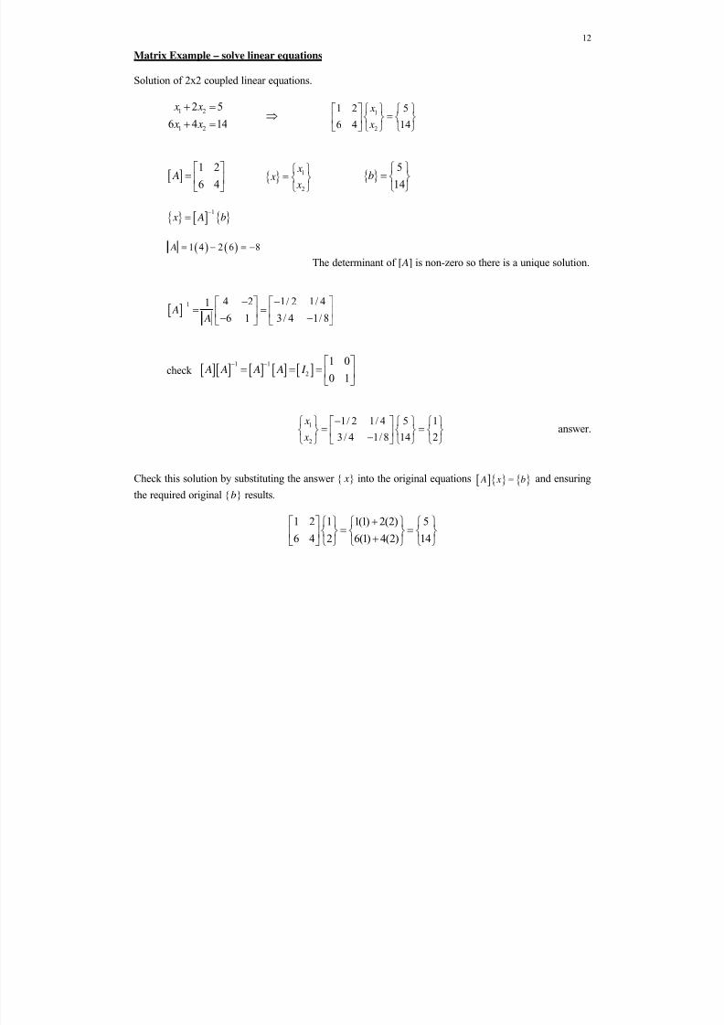
Matrix Example – solve linear equations
Solution of 2x2 coupled linear equations.
1 2
1 2
2 5
6 4 14
x x
x x
1
2
1 2 5
6 4 14
x
x
1 2
6 4 A
1
2
x x
x
5
14b
1
x A b
1 4 2 6 8 A
The determinant of [ A] is non-zero so there is a unique solution.
1 4 2 1/ 2 1/ 41
6 1 3/ 4 1/ 8 A
A
check 1 1
2
1 0
0 1 A A A A I
1
2
1/ 2 1/ 4 5 1
3/ 4 1/ 8 14 2
x
x
answer.
Check this solution by substituting the answer { x} into the original equations A x b and ensuring
the required original {b} results.
1 2 1 1(1) 2(2) 5
6 4 2 6(1) 4(2) 14

8/11/2019 Mechanism kinematics & dynamics.pdf
http://slidepdf.com/reader/full/mechanism-kinematics-dynamicspdf 13/269
13
Same Matrix Examples in MATLAB
%- - - - - - - - - - - - - - - - - - - - - - - - - - - - - - -% Mat r i ces. m - mat r i x exampl es% Dr . Bob, ME 3011 %- - - - - - - - - - - - - - - - - - - - - - - - - - - - - - -
cl ear ; cl c;
A1 = di ag( [ 1 2 3] ) % 3x3 di agonal mat r i x A2 = eye( 3) % 3x3 i dent i t y mat r i x
A3 = [ 1 2; 3 4] ; % mat r i x addi t i on A4 = [ 5 6; 7 8] ;Add = A3 + A4
k = 10; % mat ri x- scal ar mul t i pl i cat i on Mul t Sca = k*A3
Tr ans = A4' % mat r i x t r anspose ( swap rows and col umns)
A5 = [ 1 2 3; 4 5 6] ; % def i ne t wo mat r i ces A6 = [ 7 8; 9 8; 7 6] ;A7 = A5*A6 % mat r i x- mat r i x mul t i pl i cat i on A8 = A6*A5
A9 = [ 1 2; 6 4] ; % mat r i x f or l i near equat i ons sol ut i on b = [ 5; 14] ; % def i ne RHS vector dA9 = det ( A9) % cal cul at e det er mi nant of A i nvA9 = i nv( A9) % cal cul at e t he i nver se of A x = i nvA9*b % sol ve l i near equat i ons x1 = x( 1) ; % ext r act answer s x2 = x( 2) ;Check = A9*x % check answer – shoul d be b xG = A9\ b % Gaussi an el i mi nat i on i s mor e ef f i ci ent
who % di spl ay t he user - creat ed var i abl eswhos % user - cr eat ed var i abl es wi t h di mensi ons
The first solution of the linear equations above uses the matrix inverse. To solve linearequations, Gaussian Elimination is more efficient (more on this in the dynamics notes later) and morerobust numerically; Gaussian elimination implementation is given in the third to the last line of theabove m-file (with the back-slash).
Since the equations are linear, there is a unique solution (assuming the equations are linearlyindependent, i.e. the matrix is not near a singularity) and so both solution methods will yield the sameanswer.
8/11/2019 Mechanism kinematics & dynamics.pdf
http://slidepdf.com/reader/full/mechanism-kinematics-dynamicspdf 14/269
14
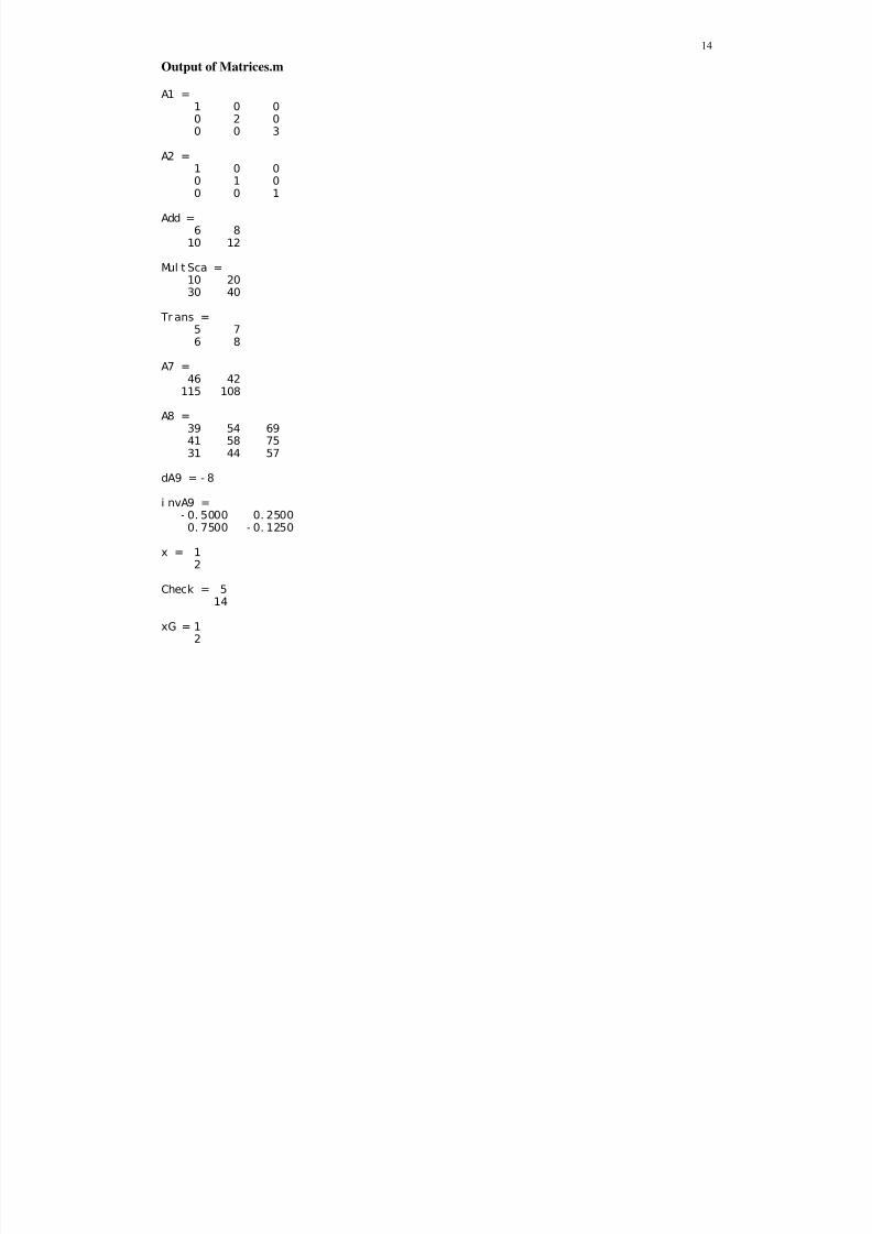
Output of Matrices.m
A1 =1 0 00 2 00 0 3
A2 =
1 0 00 1 00 0 1
Add =6 8
10 12
Mul t Sca =10 2030 40
Tr ans =
5 76 8
A7 =46 42
115 108
A8 =39 54 6941 58 7531 44 57
dA9 = - 8
i nvA9 =- 0. 5000 0. 25000. 7500 - 0. 1250
x = 12
Check = 514
xG = 12

8/11/2019 Mechanism kinematics & dynamics.pdf
http://slidepdf.com/reader/full/mechanism-kinematics-dynamicspdf 15/269
15
2. Kinematics Analysis
2.1 Position Kinematics Analysis
2.1.1 Four-Bar Mechanism Position Analysis
2.1.1.1 Tangent Half-Angle Substitution Derivation and Alternate Solution Method
Tangent half-angle substitution derivation
In this subsection we first derive the tangent half-angle substitution using ananalytical/trigonometric method. Defining parameter t to be
tan2
t
i.e. the tangent of half of the unknown angle , we need to derive cos and sin as functions of parameter t . This derivation requires the trigonometric sum of angles formulae.
cos( ) cos cos sin sin
sin( ) sin cos cos sin
a b a b a b
a b a b a b
To derive the cos term as a function of t , we start with
cos cos2 2
The cosine sum of angles formula yields
2 2cos cos sin2 2
Multiplying by a ‘1’, i.e. 2cos2
over itself yields
2 2
2 2 2
2
cos sin
2 2cos cos 1 tan cos2 2 2
cos2
The cosine squared term can be divided by another ‘1’, i.e. 2 2cos sin 12 2
.

8/11/2019 Mechanism kinematics & dynamics.pdf
http://slidepdf.com/reader/full/mechanism-kinematics-dynamicspdf 16/269
16
2
2
2 2
cos2
cos 1 tan2
cos sin2 2
Dividing top and bottom by2
cos 2
yields
2
2
1cos 1 tan
21 tan
2
Remembering the earlier definition for t , this result is the first derivation we need, i.e.
2
21cos1
t t
To derive the sin term as a function of t , we start with
sin sin2 2
The sine sum of angles formula yields
sin sin cos cos sin 2sin cos2 2 2 2 2 2
Multiplying top and bottom by cosine yields
2 2
sin2
sin 2 cos 2 tan cos2 2 2
cos
2
From the first derivation we learned
2
2
1cos
21 tan
2
8/11/2019 Mechanism kinematics & dynamics.pdf
http://slidepdf.com/reader/full/mechanism-kinematics-dynamicspdf 17/269
17
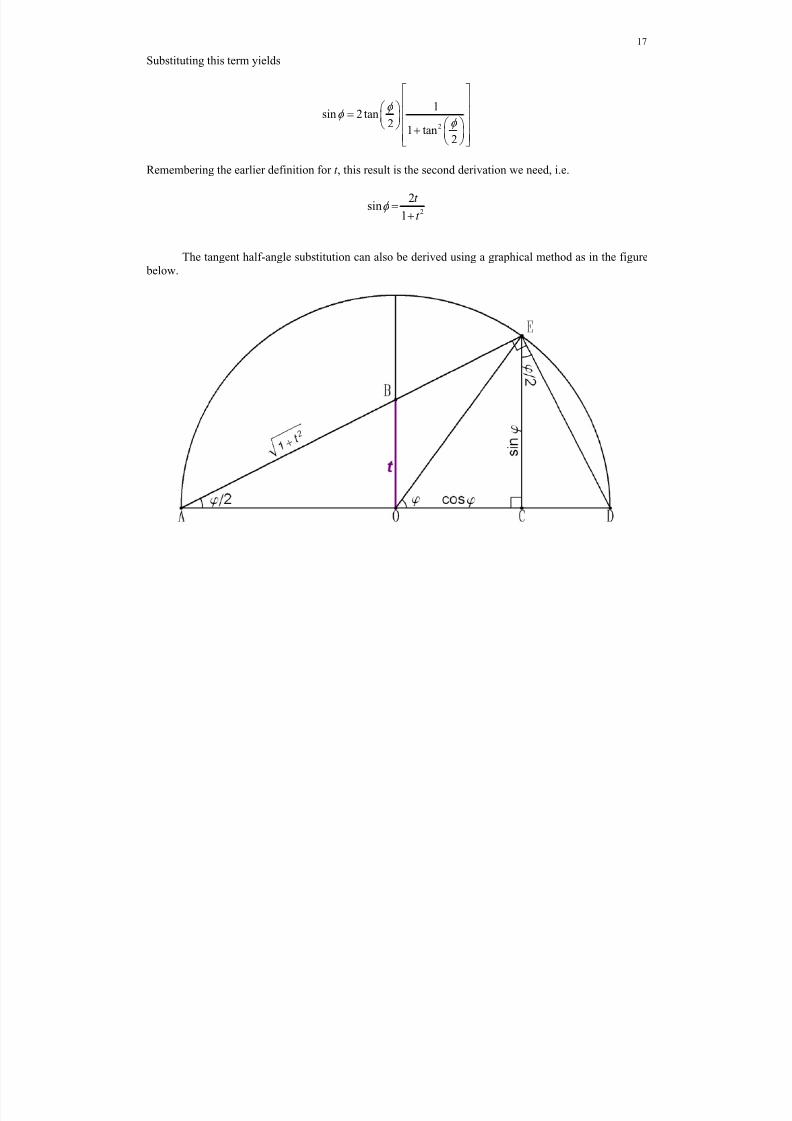
Substituting this term yields
2
1sin 2 tan
21 tan
2
Remembering the earlier definition for t , this result is the second derivation we need, i.e.
2
2sin
1
t
t
The tangent half-angle substitution can also be derived using a graphical method as in the figure below.
8/11/2019 Mechanism kinematics & dynamics.pdf
http://slidepdf.com/reader/full/mechanism-kinematics-dynamicspdf 18/269
18
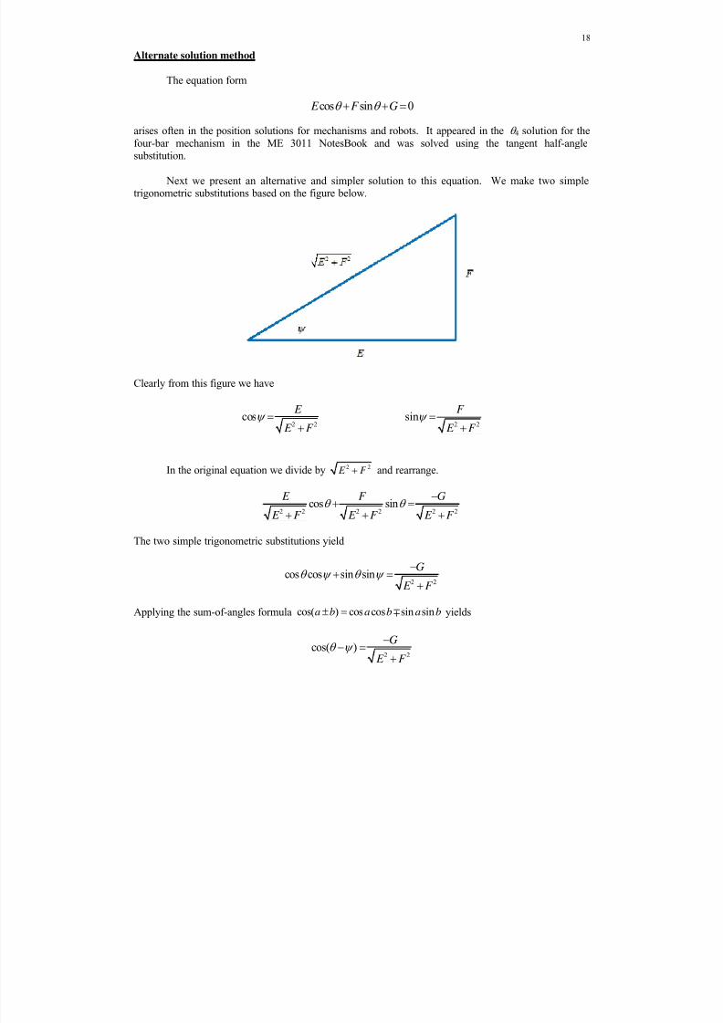
Alternate solution method
The equation form
cos sin 0 E F G
arises often in the position solutions for mechanisms and robots. It appeared in the 4 solution for thefour-bar mechanism in the ME 3011 NotesBook and was solved using the tangent half-anglesubstitution.
Next we present an alternative and simpler solution to this equation. We make two simpletrigonometric substitutions based on the figure below.
Clearly from this figure we have
2 2cos E
E F
2 2sin F
E F
In the original equation we divide by 2 2 E F and rearrange.
2 2 2 2 2 2cos sin
E F G
E F E F E F
The two simple trigonometric substitutions yield
2 2cos cos sin sin
G
E F
Applying the sum-of-angles formula cos( ) cos cos sin sina b a b a b yields
2 2cos( )
G
E F

8/11/2019 Mechanism kinematics & dynamics.pdf
http://slidepdf.com/reader/full/mechanism-kinematics-dynamicspdf 19/269
19
And so the solution for is
1
1,22 2
cos G
E F
where
1tan F
E
and the quadrant-specific inverse tangent function atan2 must be used in the above expression for .
There are two solutions for , indicated by the subscripts 1,2, since the inverse cosine function isdouble-valued. Both solutions are correct. We expected these two solutions from the tangent-half-anglesubstitution approach. They correspond to the open- and crossed-branch solutions (the engineer must
determine which is which) to the four-bar mechanism position analysis problem.
For real solutions for to exist, we must have
2 21 1
G
E F
or
2 21 1
G
E F
If this condition is violated for the four-bar mechanism, this means that the given input angle 2 is beyond its reachable limits (see Grashof’s Law).
8/11/2019 Mechanism kinematics & dynamics.pdf
http://slidepdf.com/reader/full/mechanism-kinematics-dynamicspdf 20/269
20
2.1.1.3 Four-Bar Mechanism Solution Irregularities
Four-bar mechanism position singularity 0G E
4 1 1 2 2
2 2 2 2
1 2 3 4 1 2 1 2
2 ( )
2 cos( )
E r r c r c
G r r r r r r
For simplicity, let 1 = 0 (just rotate the entire four-bar mechanism model for zero ground link angle).
2 2 2 2
1 2 3 4 1 4 2 4 1 22 2 ( ) 0G E r r r r r r r r r c
I have encountered two example four-bar mechanisms with this 0G E singularity.
Case 1
When 1 4r r and 2 3
r r , 2 2 2 2 2
1 2 2 1 1 2 1 1 22 2 ( ) 0G E r r r r r r r r c ALWAYS, regardless
of 2.
ExampleGiven 1 2 3 410, 6, 6, 10r r r r ; this mechanism is ALWAYS singular. To fix this let
1 2 3 410, 5.9999, 6.0001, 10r r r r and MATLAB will be able to calculate the position
analysis reliably at every input angle.
Case 2
When 1 32r r and 4 22r r , and furthermore 3 23 5r r ,
2 2 2 2
3 2 3 2 2 3 2 2 3 2
2 2 2 2 2 2
2 2 2 2 2 2 2
2
2 2
4 4 8 4 ( )c
100 25 40 84 c
9 9 3 3
8c
3
G E r r r r r r r r r
r r r r r r
r
This 0G E occurs only when2 90 . Case 2 is much less general than case 1.
Example
Given 1 2 3 410, 3, 5, 6r r r r ; this mechanism is singular when2 90 . To fix this ignore
290 or set your
2 array to avoid these values.
8/11/2019 Mechanism kinematics & dynamics.pdf
http://slidepdf.com/reader/full/mechanism-kinematics-dynamicspdf 21/269
21
2.1.1.4 Grashof’s Law and Four-Bar Mechanism Joint Limits
Grashof’s Law
Grashof’s Law was presented in the ME 3011 NotesBook to determine the input and output linkrotatability in a four-bar mechanism. Applying Grashof’s Law we determine if the input and output
links are a crank (C) or a rocker (R). A crank enjoys full 360 degree rotation while a rocker has arotation that is a subset of this full rotation. This section presents more information on Grashof’s Lawand then the next subsection presents four-bar mechanism joint limits.
Grashof's condition states "For a four-bar mechanism, the sum of the shortest and longest linklengths should not be greater than the sum of two remaining link lengths". With a given four-bar
mechanism, the Grashof Condition is satisfied if L S P Q where S and L are the lengths of the
shortest and longest links, and P and Q are the lengths of the other two intermediate-sized links. If theGrashof condition is satisfied, at least one link will be fully rotatable, i.e. can rotate 360 degrees.
For a four-bar mechanism, the following inequalities must be satisfied to avoid locking of the
mechanism for all motion.
2 1 3 4
4 1 2 3
r r r r
r r r r
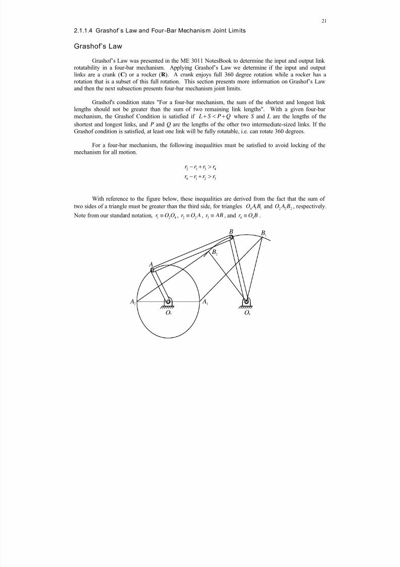
With reference to the figure below, these inequalities are derived from the fact that the sum of
two sides of a triangle must be greater than the third side, for triangles 4 1 1O A B and 2 2 2
O A B , respectively.
Note from our standard notation, 1 2 4r O O , 2 2r O A , 3r AB , and 4 4r O B .
A
B
A
O
2
2 O4
A1
B1
B2
8/11/2019 Mechanism kinematics & dynamics.pdf
http://slidepdf.com/reader/full/mechanism-kinematics-dynamicspdf 22/269
22
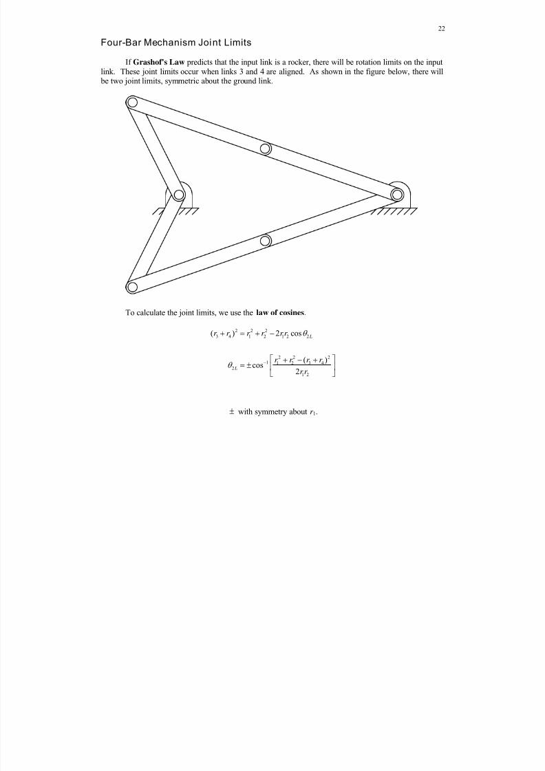
Four-Bar Mechanism Joint Limits
If Grashof's Law predicts that the input link is a rocker, there will be rotation limits on the inputlink. These joint limits occur when links 3 and 4 are aligned. As shown in the figure below, there will be two joint limits, symmetric about the ground link.
To calculate the joint limits, we use the law of cosines.
2 2 2
3 4 1 2 1 2 2
2 2 21 1 2 3 4
2
1 2
( ) 2 cos
( )cos
2
L
L
r r r r r r
r r r r
r r
with symmetry about r 1.

8/11/2019 Mechanism kinematics & dynamics.pdf
http://slidepdf.com/reader/full/mechanism-kinematics-dynamicspdf 23/269
23
Joint Limit Example 1 Given 1 2 3 410, 6, 8, 7r r r r
L S P Q (10 6 8 7 )
so we predict only double rockers from this Non-Grashof Mechanism.
2 2 2
1 1
2
10 6 (8 7)cos cos 0.742 137.92(10)(6)
L
This method can also be used to find angular limits on link 4 when it is a rocker. In this case links 2 and3 align.
2 2 2
1 1
4
10 7 (6 8)cos cos 0.336 109.6
2(10)(7)
180 70.4 L
In this example, the allowable input and output angle ranges are:
2137.9 137.9 470.4 289.6
This example is shown graphically in the ME 3011 NotesBook, in the Grashof’s Law section (2. Non-Grashof double rocker, first inversion).
Caution The figure on the previous page does not apply in all joint limit cases. For Grashof
Mechanisms with a rocker input link, one link 2 limit occurs when links 3 and 4 fold upon each otherand the other link 2 limit occurs when links 3 and 4 stretch out in a straight line. See Example 4 (andExample 3 for a similar situation with the output link 4 limits).

8/11/2019 Mechanism kinematics & dynamics.pdf
http://slidepdf.com/reader/full/mechanism-kinematics-dynamicspdf 24/269
24
Joint Limit Example 2 Given 1 2 3 410, 4, 8, 7r r r r
L S P Q (10 4 8 7 )
Since the S link is adjacent to the fixed link, we predict this Grashof Mechanism is a crank-rocker.
Therefore, there are no 2 joint limits.
2 2 2
1 1
2
10 4 (8 7)cos cos 1.3625
2(10)(4) L
which is undefined, thus confirming there are no 2 joint limits.
There are limits on link 4 since it is a rocker. For 4min, links 2 and 3 are stretched in a straight line(their absolute angles are identical).
2 2 21 1
4min
10 7 (4 8)cos cos 0.036 88.02(10)(7)
180 92.0
For 4max, links 2 and 3 are instead folded upon each other (their absolute angles are different by ).
2 2 2
1 1
4min
10 7 ( 4 8)cos cos 0.95 18.2
2(10)(7)
180 161.8
In this example, the output angle range is
492.0 161.8
and 2 is not limited. This example is shown graphically in the ME 3011 NotesBook, in the Grashof’s
Law section (1a. Grashof crank-rocker).
8/11/2019 Mechanism kinematics & dynamics.pdf
http://slidepdf.com/reader/full/mechanism-kinematics-dynamicspdf 25/269
25
Joint Limit Example 3 Given 1 2 3 411.18, 3, 8, 7r r r r (in) and1 10.3
L S P Q (11.18 3 8 7 )
This is the four-bar mechanism from Term Example 1 and it is a four-bar crank-rocker Grashof
Mechanism. There are no limits on 2 since link 2 is a crank.
The 4 limits are
4 120.1 L (links 2 and 3 stretched in a line)
4 172.5 L
(links 2 and 3 folded upon each other in a line)
The output angle range is
4120.1 172.5
and 2 is not limited. This example is NOT shown graphically in the ME 3011 NotesBook Grashof’s
Law section. However, these 4 limits are clearly seen in the F.R.O.M. plot for angle 4 in TermExample 1 in the ME 3011 NotesBook.
8/11/2019 Mechanism kinematics & dynamics.pdf
http://slidepdf.com/reader/full/mechanism-kinematics-dynamicspdf 26/269
26
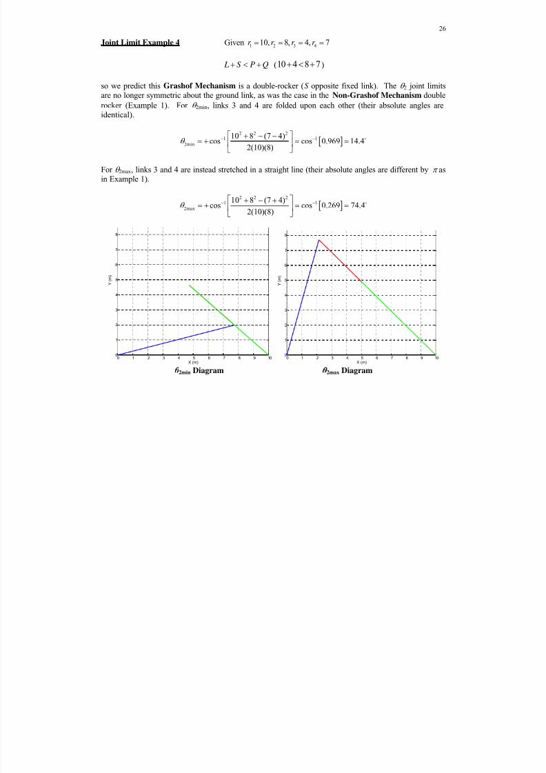
Joint Limit Example 4 Given 1 2 3 410, 8, 4, 7r r r r
L S P Q (10 4 8 7 )
so we predict this Grashof Mechanism is a double-rocker (S opposite fixed link). The 2 joint limitsare no longer symmetric about the ground link, as was the case in the Non-Grashof Mechanism double
rocker (Example 1). For 2min, links 3 and 4 are folded upon each other (their absolute angles areidentical).
2 2 2
1 1
2min
10 8 (7 4)cos cos 0.969 14.4
2(10)(8)
For 2max, links 3 and 4 are instead stretched in a straight line (their absolute angles are different by asin Example 1).
2 2 21 1
2max
10 8 (7 4)
cos cos 0.269 74.42(10)(8)
2min Diagram2max Diagram
0 1 2 3 4 5 6 7 8 9 100
1
2
3
4
5
6
7
8
X (m)
Y ( m )
0 1 2 3 4 5 6 7 8 9 100
1
2
3
4
5
6
7
8
X (m)
Y ( m )
8/11/2019 Mechanism kinematics & dynamics.pdf
http://slidepdf.com/reader/full/mechanism-kinematics-dynamicspdf 27/269
27
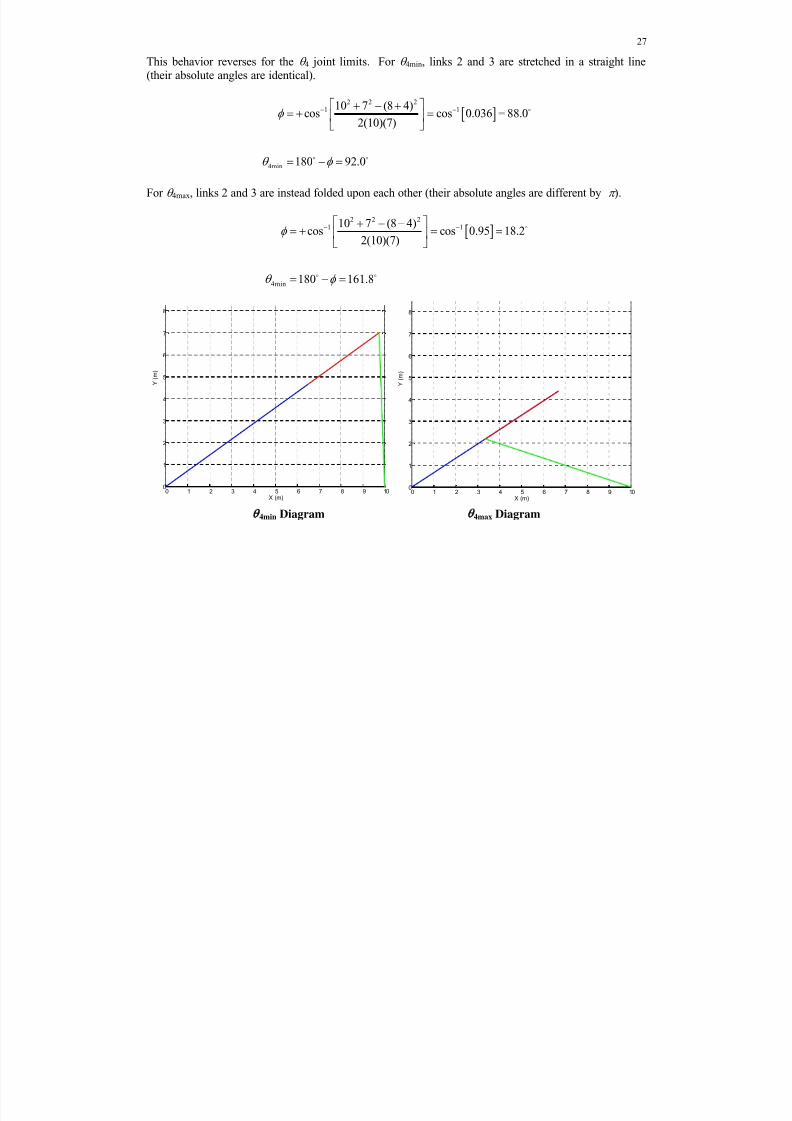
This behavior reverses for the 4 joint limits. For 4min, links 2 and 3 are stretched in a straight line(their absolute angles are identical).
2 2 2
1 1
4min
10 7 (8 4)cos cos 0.036 88.0
2(10)(7)
180 92.0
For 4max, links 2 and 3 are instead folded upon each other (their absolute angles are different by ).
2 2 2
1 1
4min
10 7 (8 4)cos cos 0.95 18.2
2(10)(7)
180 161.8
4min Diagram4max Diagram
0 1 2 3 4 5 6 7 8 9 100
1
2
3
4
5
6
7
8
X (m)
Y ( m )
0 1 2 3 4 5 6 7 8 9 100
1
2
3
4
5
6
7
8
X (m)
Y ( m )
8/11/2019 Mechanism kinematics & dynamics.pdf
http://slidepdf.com/reader/full/mechanism-kinematics-dynamicspdf 28/269
28
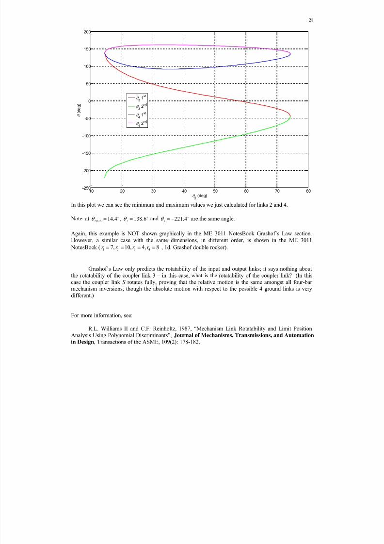
In this plot we can see the minimum and maximum values we just calculated for links 2 and 4.
Note at 2min 14.4
, 3 138.6
and 3 221.4
are the same angle.
Again, this example is NOT shown graphically in the ME 3011 NotesBook Grashof’s Law section.However, a similar case with the same dimensions, in different order, is shown in the ME 3011
NotesBook ( 1 2 3 47, 10, 4, 8r r r r , 1d. Grashof double rocker).
Grashof’s Law only predicts the rotatability of the input and output links; it says nothing aboutthe rotatability of the coupler link 3 – in this case, what is the rotatability of the coupler link? (In thiscase the coupler link S rotates fully, proving that the relative motion is the same amongst all four-barmechanism inversions, though the absolute motion with respect to the possible 4 ground links is very
different.)
For more information, see:
R.L. Williams II and C.F. Reinholtz, 1987, “Mechanism Link Rotatability and Limit PositionAnalysis Using Polynomial Discriminants”, Journal of Mechanisms, Transmissions, and Automation
in Design, Transactions of the ASME, 109(2): 178-182.
10 20 30 40 50 60 70 80-250
-200
-150
-100
-50
0
50
100
150
200
2 (deg)
( d e g )
3 1
st
3 2
nd
4 1
st
4 2
nd

8/11/2019 Mechanism kinematics & dynamics.pdf
http://slidepdf.com/reader/full/mechanism-kinematics-dynamicspdf 29/269
29
2.1.2 Slider-Crank Mechanism Posi tion Analys is
Step 6. Solve for the unknowns – alternate solution
Here are the same slider-crank mechanism position analysis XY component equations, rearranged
to isolate the 3 terms.
3 3 2 2
3 3 2 2
r c x r c
r s h r s
We can square and add to eliminate 3, similar to the four-bar mechanism solution approach.
2 2 2 2 2
3 3 2 2 2 2
2 2 2 2 2
3 3 2 2 2 2
2
2
r c x xr c r c
r s h hr s r s
2 2 2 2
3 2 2 2 2 22 2r x h r xr c hr s
This quadratic equation in x has the following form:
2 0ax bx c 2 2
2 2 2
2 3 2 2
1
2
2
a
b r c
c r r h hr s
There are two solutions for x, corresponding to the right and left branches.
2 2 2 2
1,2 2 2 3 2 2 2 22 x r c r h r s hr s
Then 3 is found from a ratio of the Y to X equations.
1,23 2 2 1,2 2 2atan2( , )h r s x r c
This alternate solution yields identical results as the earlier solution approach in the ME 3011 NotesBook for the right (
13 1, x ) and left (23 2, x ) branches.

8/11/2019 Mechanism kinematics & dynamics.pdf
http://slidepdf.com/reader/full/mechanism-kinematics-dynamicspdf 30/269
30
Slider-Crank Mechanism Snapshot and F.R.O.M. MATLAB m-files
No sample m-files are given in the ME 3011 NotesBook for the slider-crank mechanism sinceyou can readily adapt the snapshot and F.R.O.M. m-files given for the four-bar mechanism previously.
However, below we include a partial m-file to show how to draw the slider and fixed pistonwalls for the slider-crank mechanism graphics, since this was not required for the four-bar mechanism.
Outside the loop:
Lp = put a number here; % length of piston (slider link) Hp = put a number here; % height of piston Xp = [-1 -1 1 1]*Lp/2;Yp = [-1 1 1 -1]*Hp/2;
This establishes the rectangular corner coordinates for the slider link, centered at the origin of yourcoordinate frame. It can be done once, outside the loop. Instead of typing numbers for Lp and Hp, I
scale them to a fraction of r 2, for generality in different-sized slider-crank mechanisms. Note I onlyincluded the four corner points – MATLAB patch (below) closes the rectangular figure, i.e. back to
the starting point.
Inside the loop (right after the plot command where links 2 and 3 are drawn to the screen)
patch(Xp+x(i),Yp+h,'g'); % draw piston to screen
where x(i) is the variable horizontal slider displacement and h is the constant vertical offset. These
position parameters shift the piston coordinates from the origin to the correct location in each loop. Youcan use any piston color you like (I show green here, 'g').
Further, to draw the horizontal lines representing the piston walls:
Outside the loop
Xpt = [-1000 1000]; % fixed piston walls Ypt = [h+wall/2 h+wall/2];Xpb = [-1000 1000];Ypb = [h-wall/2 h-wall/2];
Inside the loop (right after the plot command where links 2 and 3 are drawn to the screen)
line(Xpt,Ypt,'LineWidth',2); line(Xpb,Ypb,'LineWidth',2);
Set the piston wall width wall to allow a small clearance between the piston and the walls. Again, it
can be scaled to a small fraction of r 2 for generality. The -1000 and 1000 coordinates used above are
to extend the piston wall lines off the screen to the left and to the right.

8/11/2019 Mechanism kinematics & dynamics.pdf
http://slidepdf.com/reader/full/mechanism-kinematics-dynamicspdf 31/269
31
MATLAB subplot feature
In a slider-crank mechanism full-range-of-motion (F.R.O.M.) simulation you will need to plot
both 3 and x vs. the independent variable 2. Since the units of 3 (deg) and x (m) are dissimilar, theymay not fit clearly on the same plot. In this situation you should use a sub-plot arrangement.
Outside the F.R.O.M. loop you can do the subplot in this way:
subplot(211); % 2x1 arrangement of plots, first plot plot(th2/DR,th3/DR);subplot(212); % 2x1 arrangement of plots, second plot plot(th2/DR,x);
Now, you can use the standard axis labels, linetypes, titles, axis limits, grid, etc., for each plot within asubplot (repeat these formatting commands after each plot statement above to use similar formatting
for each). These options are not shown, for clarity.
The generalized usage of subplot is shown below.
subplot(mni); % m x n arrangement of plots, ith plot plot( . . . );
As seen in the example syntax above, the integers need not be separated by spaces or commas.However, I believe they may be so separated if you desire.
8/11/2019 Mechanism kinematics & dynamics.pdf
http://slidepdf.com/reader/full/mechanism-kinematics-dynamicspdf 32/269
32
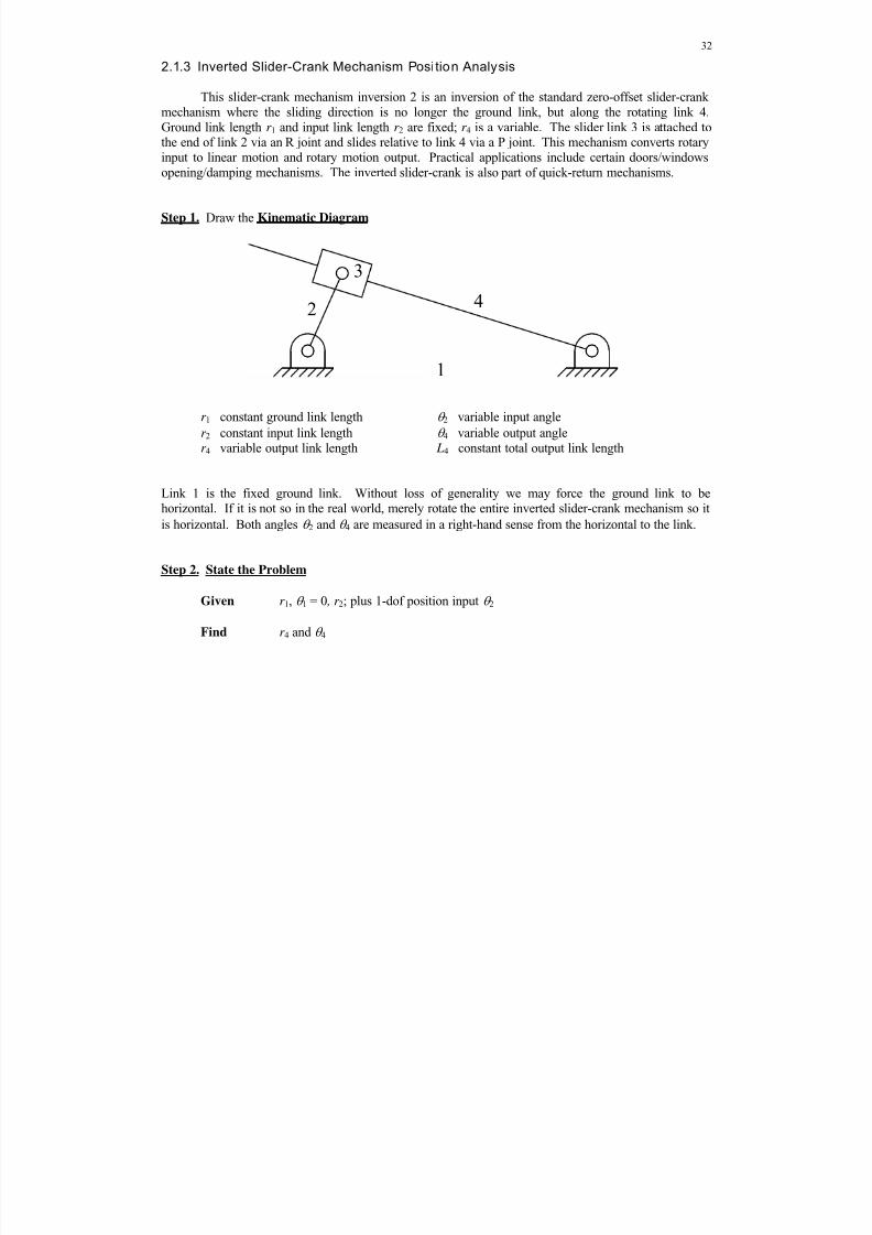
2.1.3 Inverted Slider-Crank Mechanism Posi tion Analysis
This slider-crank mechanism inversion 2 is an inversion of the standard zero-offset slider-crankmechanism where the sliding direction is no longer the ground link, but along the rotating link 4.Ground link length r 1 and input link length r 2 are fixed; r 4 is a variable. The slider link 3 is attached tothe end of link 2 via an R joint and slides relative to link 4 via a P joint. This mechanism converts rotaryinput to linear motion and rotary motion output. Practical applications include certain doors/windowsopening/damping mechanisms. The inverted slider-crank is also part of quick-return mechanisms.
Step 1. Draw the Kinematic Diagram
r 1 constant ground link length 2 variable input angle
r 2 constant input link length 4 variable output angler 4 variable output link length L4 constant total output link length
Link 1 is the fixed ground link. Without loss of generality we may force the ground link to behorizontal. If it is not so in the real world, merely rotate the entire inverted slider-crank mechanism so it
is horizontal. Both angles 2 and 4 are measured in a right-hand sense from the horizontal to the link.
Step 2. State the Problem
Given r 1, 1 = 0 , r 2; plus 1-dof position input 2
Find r 4 and 4
2
1
4
3

8/11/2019 Mechanism kinematics & dynamics.pdf
http://slidepdf.com/reader/full/mechanism-kinematics-dynamicspdf 33/269
33
Step 3. Draw the Vector Diagram. Define all angles in a positive sense, measured with the right handfrom the right horizontal to the link vector (tail-to-head; your right-hand thumb is located at the vectortail).
Step 4. Derive the Vector-Loop-Closure Equation. Starting at one point, add vectors tail-to-head untilyou reach a second point. Write the VLCE by starting and ending at the same points, but choosing adifferent path.
2 1 4r r r
Step 5. Write the XY Components for the Vector-Loop-Closure Equation. Separate the one vectorequation into its two X and Y scalar components.
2 2 1 4 4
2 2 4 4
r c r r c
r s r s
Step 6. Solve for the Unknowns from the XY equations. There are two coupled nonlinear equations in
the two unknowns r 4,
4. Unlike the standard slider-crank mechanism, there is no decoupling of X and
Y . However, unlike the four-bar mechanism, there is only one unknown angle so the solution is easierthan the four-bar mechanism. First rewrite the above XY equations to isolate the unknowns on one side.
4 4 2 2 1
4 4 2 2
r c r c r
r s r s
A ratio of the Y to X equations will cancel r 4 and solve for 4.
4 4 2 2
4 4 2 2 1
r s r s
r c r c r
4 2 2 2 2 1atan2( , )r s r c r
Then square and add the XY equations to eliminate 4 and solve for r 4.
2 2
4 1 2 1 2 22r r r rr c
2
1
4

8/11/2019 Mechanism kinematics & dynamics.pdf
http://slidepdf.com/reader/full/mechanism-kinematics-dynamicspdf 34/269
34
Note the same r 4 formula results from the cosine law. Alternatively, the same r 4 can be solved from
either the X or Y equations after is 4 known.
X ) 2 2 14
4
r c r r
c
Y ) 2 2
4
4
r sr
s
Both of these r 4 alternatives are valid; however, each is subject to a different artificial mathematicalsingularity (
4 90 and4 0,180 , respectively), so only the former square-root formula should be
used for r 4, which has no artificial singularity. The X algorithmic singularity4 90 never occurs
unless 2 1r r , which is to be avoided (see below), but the Y algorithmic singularity occurs twice per full
range of motion.
Technically there are two solution sets – the one above and2 2
4 1 2 1 2 22r r r rr c , 4 .
However, the negative r 4 is not practical and so only the one solution set (branch) exists, unlike most planar mechanisms with two or more branches.
Full-rotation condition
For the inverted slider-crank mechanism to rotate fully, the fixed length of link 4, L4, must begreater than the maximum value of the variable r 4.
Slider Limits
The slider reaches its minimum and maximum displacements when 2 = 0 and , respectively.
Therefore, the slider limits are 1 2 4 1 2r r r r r . Thus, the fixed length L4 must be greater than 1 2r r .In addition we require 1 2r r for full rotation.

8/11/2019 Mechanism kinematics & dynamics.pdf
http://slidepdf.com/reader/full/mechanism-kinematics-dynamicspdf 35/269
35
Graphical Solution
The Inverted Slider-Crank mechanism position analysis may be solved graphically, by drawingthe mechanism, determining the mechanism closure, and measuring the unknowns. This is an excellentmethod to validate your computer results at a given snapshot.
Draw the known ground link (points O2 and O4 separated by r 1 at the fixed angle 1 = 0).
Draw the given input link length r 2 at the given angle 2 (this defines point A).
Draw a line from O4 to point A.
Measure the unknown values of r 4 and 4.

8/11/2019 Mechanism kinematics & dynamics.pdf
http://slidepdf.com/reader/full/mechanism-kinematics-dynamicspdf 36/269

8/11/2019 Mechanism kinematics & dynamics.pdf
http://slidepdf.com/reader/full/mechanism-kinematics-dynamicspdf 37/269
37
Full-Range-Of-Motion (F.R.O.M.) Analysis: Term Example 3
A more meaningful result from position analysis is to report the position analysis unknowns for
the entire range of mechanism motion. The subplots below gives r 4 (m) and 4 (deg), for all
20 360 , for Term Example 3.
Term Example 3 4 and r4
4 varies symmetrically about 180 , being 180
at2 0,180,360 . r 4 varies like a negative cosine
function with minimum displacement 1 2 0.1r r at2 0,360 and maximum displacement 1 2 0.3r r
. Since r 1 is twice r 2 in this example, whenever2 60,300 , a perfect 30 60 90
triangle is
formed; the relative angle between links 2 and 4 is 90 which corresponds to the max and min of
4 150,210 , respectively. At these special points, 4 ( 3 2)0.2 0.173r m.
There is another right triangle that shows up for2 90 ; in these cases
2 2
4 0.2 0.1 0.224r m and4 153.4,206.6 , respectively. Check all of these special values in the
F.R.O.M. plot results.
0 50 100 150 200 250 300 350150
160
170
180
190
200
210
4 ( d e g )
0 50 100 150 200 250 300 3500.1
0.15
0.2
0.25
0.3
2 (deg)
r 4
m

8/11/2019 Mechanism kinematics & dynamics.pdf
http://slidepdf.com/reader/full/mechanism-kinematics-dynamicspdf 38/269
38
2.1.4 Multi-Loop Mechanism Position Analysis
Thus far we have presented position analysis for the single-loop four-bar, slider-crank, andinverted slider-crank mechanisms. The position analysis for mechanisms of more than one loop ishandled using the same general procedures developed for the single loop mechanisms. A good rule ofthumb is to look for four-bar (or slider-crank) parts of the multi-loop mechanism as we already knowhow to solve the complete position analyses for these.
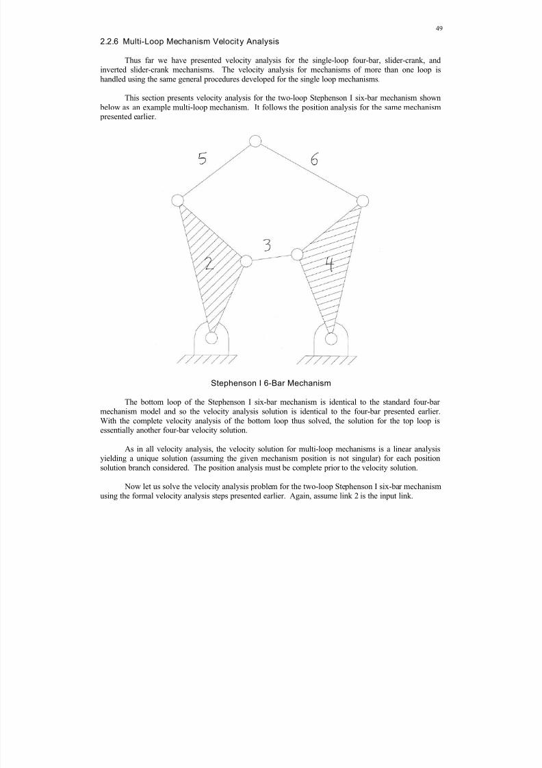
This section presents position analysis for the two-loop Stephenson I six-bar mechanism shown below as an example multi-loop mechanism. This is one of the five possible six-bar mechanisms shownin the on-line Mechanisms Atlas.
Stephenson I 6-Bar Mechanism
We immediately see that the bottom loop of the Stephenson I six-bar mechanism is identical toour standard four-bar mechanism model. Since we number the links the same as in the four-bar, and ifwe define the angles identically, the position analysis solution is identical to the four-bar presentedearlier. With the complete position analysis of the bottom loop thus solved, we see that points C and D can be easily calculated. Then the solution for the top loop is essentially another four-bar solution:graphically, the circle of radius r 5 about point C must intersect the circle of radius r 6 about point D toform point E (yielding two possible intersections in general). The analytical solution is very similar tothe standard four-bar position solution, as we will show.
For multi-loop mechanisms, the number of solution branches for position analysis increasescompared to the single-loop mechanisms. Most single-loop mechanisms mathematically have twosolution branches. For multi-loop mechanisms composed of multiple single-loop mechanisms, thenumber of solution branches is 2n, where n is the number of mechanism loops. For the two-loopStephenson I six-bar mechanism, the number of solution branches for the position analysis problem is 4,two from the standard four-bar part, and two for each of these branches from the upper loop.
8/11/2019 Mechanism kinematics & dynamics.pdf
http://slidepdf.com/reader/full/mechanism-kinematics-dynamicspdf 39/269
39
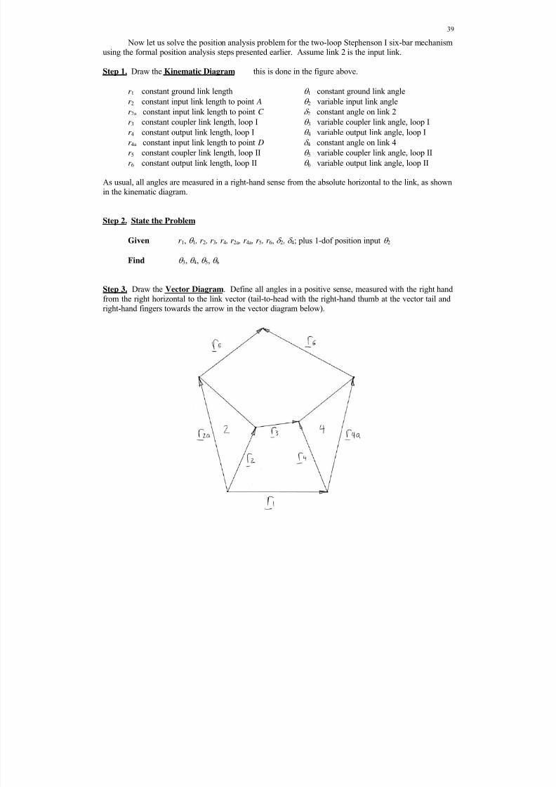
Now let us solve the position analysis problem for the two-loop Stephenson I six-bar mechanismusing the formal position analysis steps presented earlier. Assume link 2 is the input link.
Step 1. Draw the Kinematic Diagram this is done in the figure above.
r 1 constant ground link length 1 constant ground link angle
r 2
constant input link length to point A 2 variable input link angle
r 2a constant input link length to point C 2 constant angle on link 2
r 3 constant coupler link length, loop I 3 variable coupler link angle, loop I
r 4 constant output link length, loop I 4 variable output link angle, loop I
r 4a constant input link length to point D 4 constant angle on link 4
r 5 constant coupler link length, loop II 5 variable coupler link angle, loop II
r 6 constant output link length, loop II 6 variable output link angle, loop II
As usual, all angles are measured in a right-hand sense from the absolute horizontal to the link, as shownin the kinematic diagram.
Step 2. State the Problem
Given r 1, 1 , r 2 , r 3 , r 4 , r 2a , r 4a , r 5 , r 6, 2, 4; plus 1-dof position input 2
Find 3, 4, 5, 6
Step 3. Draw the Vector Diagram. Define all angles in a positive sense, measured with the right handfrom the right horizontal to the link vector (tail-to-head with the right-hand thumb at the vector tail andright-hand fingers towards the arrow in the vector diagram below).
8/11/2019 Mechanism kinematics & dynamics.pdf
http://slidepdf.com/reader/full/mechanism-kinematics-dynamicspdf 40/269
40
Step 4. Derive the Vector-Loop-Closure Equations. One VLCE is required for each mechanism loop.Start at one point, add vectors tail-to-head until you reach a second point. Write each vector equation bystarting and ending at the same points, but choosing a different path.
2 3 1 4
2 5 1 4 6a a
r r r r
r r r r r
Note an alternative to the second vector loop equation is 2 5 3 4 6b br r r r r . See if you can identify
2br and 4br , plus their angles 2b and 4b.
Step 5. Write the XY Components for each Vector-Loop-Closure Equation. Separate the two vectorequations into four XY scalar component equations.
2 2 3 3 1 1 4 4
2 2 3 3 1 1 4 4
r c r c rc r cr s r s r s r s
2 2 5 5 1 1 4 4 6 6
2 2 5 5 1 1 4 4 6 6
a a a a
a a a a
r c r c rc r c r c
r s r s r s r s r s
where2 2 2
4 4 4
a
a
Step 6. Solve for the Unknowns from the four XY Equations. The four coupled nonlinear equations in
the four unknowns 3, 4, 5, 6 can be solved in two stages, one for each mechanism loop.
Loop I. This solution is identical to the standard four-bar mechanism solution for 3, 4,
summarized here from earlier. From the first two XY scalar equations above, isolate 3 terms, square
and add both equations to obtain one equation in one unknown 4. This equation has the form
4 4cos sin 0 E F G , where terms E , F , and G are known functions of constants and the input angle
2. Solve this equation for two possible values of 4 using the tangent half-angle substitution. The two
4 values correspond to the open and crossed branches. Then return to the original XY scalar equations
with 3 terms isolated, divide the Y by the X equations, and solve for 3 using the atan2 function,substituting the solved values for 4. One unique 3 will result for each of the two possible 4 values.
Loop II. The method is analogous to the Loop I solution above. Since 4 is now known, we also
know 4 4 4a . From the second two XY scalar equations above, isolate 5 terms, square and add
both equations to obtain one equation in one unknown 6. This equation is of the form
2 6 2 6 2cos sin 0 E F G , where terms E 2, F 2, and G2 are known functions of constants and the known
angles 2 2 2a and 4 4 4a . Solve this equation for two possible values of 6 using the tangent

8/11/2019 Mechanism kinematics & dynamics.pdf
http://slidepdf.com/reader/full/mechanism-kinematics-dynamicspdf 41/269
41
half-angle substitution. The two 6 values correspond to open and crossed branches, for each of the
Loop I open and crossed branches. Then return to the original XY scalar equations with 5 terms
isolated, divide the Y by the X equations, and solve for 5 using the atan2 function, substituting the
solved values for 6. One unique 5 will result for each of the two possible 6 values from each 4.
Branches. There are two 5, 6 branches for each of the two 3, 4 branches, so there are four
overall mechanism branches for the two-loop Stephenson I six-bar mechanism.
Full-rotation condition
The range of motion of a multi-loop mechanism may be more limited than that of single-loopmechanisms. One can perform a compound Grashof analysis when four-bars are the componentmechanisms. For the two-loop Stephenson I six-bar mechanism, the second loop may constrain the firstloop (e.g. it may change an expected crank motion of the input link to a rocker). This is an importantissue in design of multi-loop mechanisms if the input link must still rotate fully.
Graphical Solution
The two-loop Stephenson I six-bar mechanism position analysis may readily be solvedgraphically, by drawing the mechanism, determining the mechanism closure, and measuring theunknowns. This is an excellent method to validate your computer results at a given snapshot.
Loop I (this part is identical to the standard four-bar graphical solution)
Draw the known ground link (points O2 and O4 separated by r 1 at the fixed angle 1).
Draw the given input link length r 2 at the given angle 2 to yield point A.
Draw a circle of radius r 3, centered at point A.
Draw a circle of radius r 4, centered at point O4. These circles intersect in general in two places to yield two possible points B.
Connect the two branches and measure the unknown angles 3 and 4.
Loop II (this part is a modification of the standard four-bar graphical solution). Start with the end of the procedure above, on the same drawing. For each solution branch above, perform the following steps.
Draw the link r 2a at angle 2 2 2a from point O2.
Draw the link r 4a at angle 4 4 4a from point O4.
Draw a circle of radius r 5, centered at point C .
Draw a circle of radius r 6, centered at point D.
These circles intersect in general in two places to yield two possible points E . Connect the two branches and measure the unknown values 5 and 6.
In general, there are four overall position solution branches.
8/11/2019 Mechanism kinematics & dynamics.pdf
http://slidepdf.com/reader/full/mechanism-kinematics-dynamicspdf 42/269
42
2.2 Veloci ty Kinematics Analysis
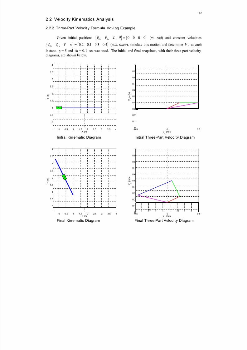
2.2.2 Three-Part Velocity Formula Moving Example
Given initial positions 0 00 0 0 0
x yP P L (m, rad ) and constant velocities
0 0 0.2 0.1 0.3 0.4
x yV V V (m/s, rad /s), simulate this motion and determine PV at each
instant. t f = 5 and 0.1t sec was used. The initial and final snapshots, with their three-part velocity
diagrams, are shown below.
Initial Kinematic Diagram Initial Three-Part Velocity Diagram
Final Kinematic Diagram Final Three-Part Velocity Diagram
0 0.5 1 1.5 2 2.5 3 3.5 4
0
0.5
1
1.5
2
2.5
3
3.5
4
X (m)
Y ( m )
-0.5 0 0.50
0.1
0.2
0.3
0.4
0.5
0.6
0.7
0.8
0.9
1
Vx (m/s)
V y
( m / s )
0 0.5 1 1.5 2 2.5 3 3.5 4
0
0.5
1
1.5
2
2.5
3
3.5
4
X (m)
Y
( m )
-0.5 0 0.50
0.1
0.2
0.3
0.4
0.5
0.6
0.7
0.8
0.9
1
Vx (m/s)
V y
( m / s )
V0
V x L
VP
8/11/2019 Mechanism kinematics & dynamics.pdf
http://slidepdf.com/reader/full/mechanism-kinematics-dynamicspdf 43/269
43
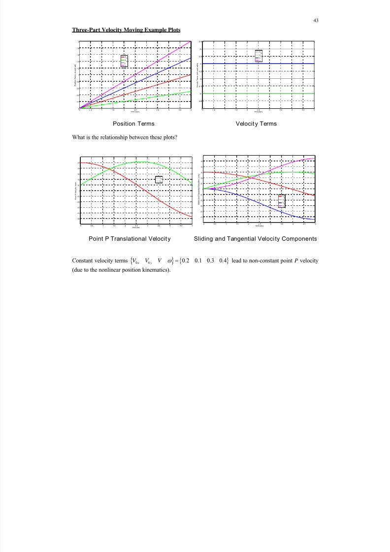
Three-Part Velocity Moving Example Plots
Position Terms Velocity Terms
What is the relationship between these plots?
Point P Translational Velocity Sliding and Tangential Veloci ty Components
Constant velocity terms 0 0 0.2 0.1 0.3 0.4 x yV V V lead to non-constant point P velocity
(due to the nonlinear position kinematics).
0 0.5 1 1.5 2 2.5 3 3.5 4 4.5 50
0.2
0.4
0.6
0.8
1
1.2
1.4
1.6
1.8
2
time (sec)
P o s i t i o n T e r m s
( m a
n d r a d )
P0x
P0y
L
0 0.5 1 1.5 2 2.5 3 3.5 4 4.5 50
0.05
0.1
0.15
0.2
0.25
0.3
0.35
0.4
0.45
time (sec)
V e l o c i t y T e r m s ( m / s a n d r a d / s )
V0x
V0y
V
0 0.5 1 1.5 2 2.5 3 3.5 4 4.5 5
-0.5
-0.4
-0.3
-0.2
-0.1
0
0.1
0.2
0.3
0.4
0.5
time (sec)
P o i n t P V e l o c i t y ( m / s )
VPx
VPy
0 0.5 1 1.5 2 2.5 3 3.5 4 4.5 5
-0.5
-0.4
-0.3
-0.2
-0.1
0
0.1
0.2
0.3
0.4
0.5
time (sec)
S l i d i n g a n d T a n g e n t i a l V e l o c i t i e s
( m / s )
Vsx
Vsy
Vtx
Vty

8/11/2019 Mechanism kinematics & dynamics.pdf
http://slidepdf.com/reader/full/mechanism-kinematics-dynamicspdf 44/269
44
2.2.3 Four-Bar Mechanism Veloci ty Analysis
The four-bar mechanism velocity solution presented in the 3011 NotesBook used the simplifyingterms a – f . Here is the solution presented in the 3011 NotesBook:
3
ce bf
ae bd
4
af cd
ae bd
3 3
4 4
2 2 2
3 3
4 4
2 2 2
a r s
b r sc r s
d r c
e r c
f r c
Backsubstituting the terms a – f yields the following equivalent solutions, which simplify nicely usingthe sum-of-angles formula sin( ) sin cos cos sina b a b a b and better display the structure of the
solutions.
2 4 23 2
3 4 3
sin( )
sin( )
r
r
2 3 24 2
4 4 3
sin( )
sin( )
r
r
These solution forms clearly show the singularity condition derived for this problem in the 3011 NotesBook, i.e. the mechanism is singular and these solutions are both infinite when:
4 3sin( ) 0 4 3 0 ,180 ,
Physically, this happens when links 3 and 4 are straight out or folded on top of each other, as explainedin the 3011 NotesBook (corresponding to joint limits on the input link 2).

8/11/2019 Mechanism kinematics & dynamics.pdf
http://slidepdf.com/reader/full/mechanism-kinematics-dynamicspdf 45/269
45
2.2.5 Inverted Slider-Crank Mechanism Velocity Analysis
Again, link 2 (the crank) is the input and link 4 is the output. Remember r 4 is a variable so
4 0r in this problem.
Step 1. The inverted slider-crank mechanism Position Analysis must first be complete.
Given r 1, 1 = 0 , r 2, and 2, we solved for r 4 and 4
Step 2. Draw the inverted slider-crank mechanism Velocity Diagram.
where i (i = 2,4) is the absolute angular velocity of link i. 4r is the slider velocity along link 4.
3 4 since the slider cannot rotate relative to link 4.
Step 3. State the Problem
Given the mechanism r 1, 1 = 0 , r 2
the position analysis 2, r 4, 4
1-dof of velocity input 2
Find the velocity unknowns 4r and 4
2
1
4
3
8/11/2019 Mechanism kinematics & dynamics.pdf
http://slidepdf.com/reader/full/mechanism-kinematics-dynamicspdf 46/269
46
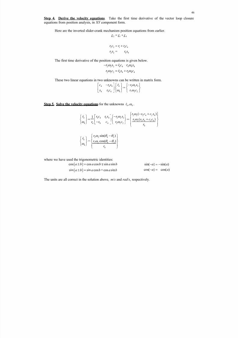
Step 4. Derive the velocity equations. Take the first time derivative of the vector loop closureequations from position analysis, in XY component form.
Here are the inverted slider-crank mechanism position equations from earlier.
2 1 4
2 2 1 4 4
2 2 4 4
r r r
r c r r c
r s r s
The first time derivative of the position equations is given below.
2 2 2 4 4 4 4 4
2 2 2 4 4 4 4 4
r s r c r s
r c r s r c
These two linear equations in two unknowns can be written in matrix form.
4 4 4 4 2 2 2
4 4 4 4 2 2 2
c r s r r s
s r c r c
Step 5. Solve the velocity equations for the unknowns 4 4,r .
2 2 2 4 2 4
4 4 4 4 4 2 2 2
2 2 2 4 2 4
4 4 4 2 2 24
4
2 2 4 24
2 2 4 2
4
4
( )1
( )
sin( )cos( )
r s c c sr r c r s r s
r s s c cs c r cr
r
r r r
r
where we have used the trigonometric identities:
cos cos cos sin sin
sin sin cos cos sin
a b a b a b
a b a b a b
sin( ) sin( )
cos( ) cos( )
a a
a a
The units are all correct in the solution above, m/s and rad /s, respectively.

8/11/2019 Mechanism kinematics & dynamics.pdf
http://slidepdf.com/reader/full/mechanism-kinematics-dynamicspdf 47/269
47
Inverted slider-crank mechanism singularity condition When does the solution fail? This is an inverted slider-crank mechanism singularity, when the
determinant of the coefficient matrix goes to zero. The result is dividing by zero, resulting in infinite
4 4,r .
4 4 4
4 4 4
c r s A
s r c
2 2 2 2
4 4 4 4 4 4 4 4( ) ( ) 0 A r c r s r c s r
Physically, assuming1 2r r as in the full rotation condition from the inverted slider-crank mechanism
position analysis, this is impossible, i.e. r 4 never goes to zero.
This matrix determinant 4 A r was used in the solution of the previous page.
Inverted slider-crank mechanism velocity example – Term Example 3 continued
Given
1
2
4
1
0.20
0.10
0.32
0
r
r
L
(m)
2
4
4
70
150.5
0.191r
(deg and m)
Snapshot AnalysisGiven this mechanism position analysis plus 2 25 rad /s, calculate 4 4,r for this snapshot.
4
4
0.870 0.094 2.349
0.493 0.166 0.855
r
4
4
2.47
2.18
r
(m/s and rad /s)
Both are positive, so the slider link 3 is currently traveling up link 4 and link 4 is currently rotating in the
ccw direction, which makes sense from the physical problem.

8/11/2019 Mechanism kinematics & dynamics.pdf
http://slidepdf.com/reader/full/mechanism-kinematics-dynamicspdf 48/269
48
Full-Range-Of-Motion (F.R.O.M.) Analysis – Term Example 3 continued
A more meaningful result from velocity analysis is to report the velocity analysis results for the
entire range of mechanism motion. The subplot below gives 4 (top, rad /s) and 4r (bottom, m/s), for all
20 360 , for Term Example 3. Since 2 is constant, we can plot the velocity results vs. 2 (since it
is related to time t via 2 2t ).
Term Example 3 F.R.O.M., 4 and 4r
As expected, 4 is zero at the max and min for 4 (at2 60 ); also, 4 has a large range of nearly
constant positive velocity near the middle of motion – this can be seen in a MATLAB animation. 4r
iszero at the beginning, middle, and end of motion and is max at
2 60 .
0 50 100 150 200 250 300 350-25
-20
-15
-10
-5
0
5
10
4
( r a d / s )
0 50 100 150 200 250 300 350
-2
-1
0
1
2
2 (deg)
r 4 d
( m / s )
8/11/2019 Mechanism kinematics & dynamics.pdf
http://slidepdf.com/reader/full/mechanism-kinematics-dynamicspdf 49/269
49
2.2.6 Multi-Loop Mechanism Velocity Analysis
Thus far we have presented velocity analysis for the single-loop four-bar, slider-crank, andinverted slider-crank mechanisms. The velocity analysis for mechanisms of more than one loop ishandled using the same general procedures developed for the single loop mechanisms.
This section presents velocity analysis for the two-loop Stephenson I six-bar mechanism shown below as an example multi-loop mechanism. It follows the position analysis for the same mechanism presented earlier.
Stephenson I 6-Bar Mechanism
The bottom loop of the Stephenson I six-bar mechanism is identical to the standard four-bar
mechanism model and so the velocity analysis solution is identical to the four-bar presented earlier.With the complete velocity analysis of the bottom loop thus solved, the solution for the top loop isessentially another four-bar velocity solution.
As in all velocity analysis, the velocity solution for multi-loop mechanisms is a linear analysisyielding a unique solution (assuming the given mechanism position is not singular) for each positionsolution branch considered. The position analysis must be complete prior to the velocity solution.
Now let us solve the velocity analysis problem for the two-loop Stephenson I six-bar mechanismusing the formal velocity analysis steps presented earlier. Again, assume link 2 is the input link.
8/11/2019 Mechanism kinematics & dynamics.pdf
http://slidepdf.com/reader/full/mechanism-kinematics-dynamicspdf 50/269
50
Step 1. The Stephenson I six-bar mechanism Position Analysis must first be complete.
Given r 1, 1 , r 2 , r 3 , r 4 , r 2a , r 4a , r 5 , r 6, 2, 4, and 2 we solved for 3, 4, 5, 6.
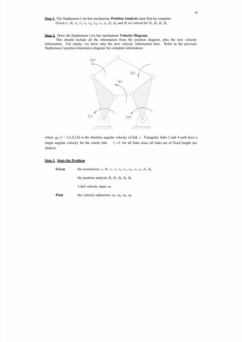
Step 2. Draw the Stephenson I six-bar mechanism Velocity Diagram.This should include all the information from the position diagram, plus the new velocity
information. For clarity, we show only the new velocity information here. Refer to the previousStephenson I position kinematics diagram for complete information.
where i (i = 2,3,4,5,6) is the absolute angular velocity of link i. Triangular links 2 and 4 each have asingle angular velocity for the whole link. 0i
r for all links since all links are of fixed length (no
sliders).
Step 3. State the Problem
Given the mechanism r 1, 1 , r 2 , r 3 , r 4 , r 2a , r 4a , r 5 , r 6, 2, 4,
the position analysis 2, 3, 4, 5, 6,
1-dof velocity input 2
Find the velocity unknowns 3, 4, 5, 6
8/11/2019 Mechanism kinematics & dynamics.pdf
http://slidepdf.com/reader/full/mechanism-kinematics-dynamicspdf 51/269
51
Step 4. Derive the velocity equations. Take the first time derivative of each of the two vector loopclosure equations from position analysis, in XY component form.
Here are the Stephenson I six-bar mechanism position equations.
Vector equations
2 3 1 4
2 5 1 4 6a a
r r r r
r r r r r
XY scalar equations
2 2 3 3 1 1 4 4
2 2 3 3 1 1 4 4
r c r c rc r c
r s r s r s r s
2 2 5 5 1 1 4 4 6 6
2 2 5 5 1 1 4 4 6 6
a a a a
a a a a
r c r c rc r c r c
r s r s r s r s r s
where2 2 2
4 4 4
a
a
The first time derivatives of the Loop I position equations are identical to those for the standardfour-bar mechanism.
2 2 2 3 3 3 4 4 4
2 2 2 3 3 3 4 4 4
r s r s r s
r c r c r c
These equations can be written in matrix form.
3 3 4 4 3 2 2 2
3 3 4 4 4 2 2 2
r s r s r s
r c r c r c
The first time derivative of the Loop II position equations is
2 2 2 5 5 5 4 4 4 6 6 6
2 2 2 5 5 5 4 4 4 6 6 6
a a a a a a
a a a a a a
r s r s r s r s
r c r c r c r c
These equations can be written in matrix form.
5 5 6 6 5 2 2 2 4 4 4
5 5 6 6 6 2 2 2 4 4 4
a a a a
a a a a
r s r s r s r s
r c r c r c r c
where we have used2 2
4 4
a
a
since 2 and 4 are constant angles.
8/11/2019 Mechanism kinematics & dynamics.pdf
http://slidepdf.com/reader/full/mechanism-kinematics-dynamicspdf 52/269
52
Step 5. Solve the velocity equations for the unknowns 3, 4, 5, 6.
The two mechanism loops decouple so we find 3 and 4 from Loop I first and then use 4 to
find 5 and 6 from Loop II. The solutions are given below.
Loop I (identical to the standard four-bar mechanism)
1
3 3 4 43 2 2 2
3 3 4 44 2 2 2
r s r s r s
r c r c r c
Loop II (similar to the standard four-bar mechanism)
1
5 5 5 6 6 2 2 2 4 4 4
6 5 5 6 6 2 2 2 4 4 4
a a a a
a a a a
r s r s r s r s
r c r c r c r c
Remember, Gaussian elimination is more efficient and robust than the matrix inverse. Also, theseequations may be solved algebraically instead of using matrix methods to yield the same answers.
Stephenson I six-bar mechanism singularity condition
The velocity solution fails when the determinant of either coefficient matrix above goes to zero.The result is dividing by zero, resulting in infinite angular velocities for the associated loop.
For the first loop, the singularity condition is identical to the singularity condition of the standardfour-bar mechanism, i.e. when links 3 and 4 either line up or fold upon each other, causing a link 2 jointlimit. For the second loop, the singularity condition is similar, occurring when links 5 and 6 either lineup or fold upon each other. These conditions also cause angle limit problems for the position analysis,so the velocity singularities are known problems.

8/11/2019 Mechanism kinematics & dynamics.pdf
http://slidepdf.com/reader/full/mechanism-kinematics-dynamicspdf 53/269
53
2.3 Acceleration Kinematics Analysis
2.3.2 Five-Part Acceleration Formula Moving Example
Given initial positions 0 0 0 0 0 0 x yP P L (m, rad ), initial velocities
0 0 0 0 0 0 x y
V V V (m/s, rad /s) and constant accelerations 0 0 x y A A A
0.2 0.05 0.15 0.1 (m/s2, rad /s2), simulate this motion and determine P A at each instant. t f = 5
and 0.1t sec was used; the initial and final snapshots, with their five-part acceleration diagrams, are
shown below.
Initial Kinematic Diagram Initial Five-Part Acceleration Diagram
Final Kinematic Diagram Final Five-Part Acceleration Diagram
0 0.5 1 1.5 2 2.5 3 3.5 4
0
0.5
1
1.5
2
2.5
3
3.5
4
X (m)
Y ( m )
-0.8 -0.2 0.40
0.2
0.4
0.6
0.8
1
1.2
A m/s2
A y
( m / s
2 )
0 0.5 1 1.5 2 2.5 3 3.5 4
0
0.5
1
1.5
2
2.5
3
3.5
4
X (m)
Y ( m )
-0.8 -0.2 0.40
0.2
0.4
0.6
0.8
1
1.2
Ax (m/s
2)
A y
( m / s
2 )
A0
A
2 x V
x L
x ( x L)
AP
8/11/2019 Mechanism kinematics & dynamics.pdf
http://slidepdf.com/reader/full/mechanism-kinematics-dynamicspdf 54/269
54
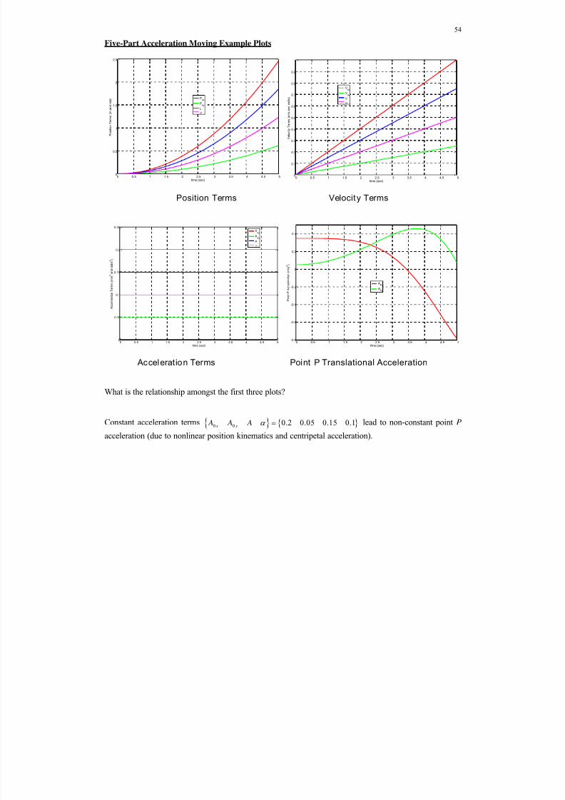
Five-Part Acceleration Moving Example Plots
Position Terms Velocity Terms
Acceleration Terms Point P Translational Acceleration
What is the relationship amongst the first three plots?
Constant acceleration terms 0 0 0.2 0.05 0.15 0.1 x y
A A A lead to non-constant point P
acceleration (due to nonlinear position kinematics and centripetal acceleration).
0 0.5 1 1.5 2 2.5 3 3.5 4 4.5 50
0.5
1
1.5
2
2.5
time (sec)
P o s i t i o n T e r m s ( m a n
d r a d )
P0x
P0y
L
0 0.5 1 1.5 2 2.5 3 3.5 4 4.5 50
0.1
0.2
0.3
0.4
0.5
0.6
0.7
0.8
0.9
1
time (sec)
V e l o c i t y T e r m s ( m / s a n d r a d / s )
V0x
V0y
V
0 0.5 1 1.5 2 2.5 3 3.5 4 4.5 50
0.05
0.1
0.15
0.2
0.25
time (sec)
A c c e l e r a t i o n T e r m s ( m / s
2 a
n d r a d / s
2 )
A0x
A0y
A
0 0.5 1 1.5 2 2.5 3 3.5 4 4.5 5-0.8
-0.6
-0.4
-0.2
0
0.2
0.4
time (sec)
P o i n t P A c c e l e r a t i o n ( m / s
2 )
APx
APy

8/11/2019 Mechanism kinematics & dynamics.pdf
http://slidepdf.com/reader/full/mechanism-kinematics-dynamicspdf 55/269
55
2.3.3 Four-Bar Mechanism Acceleration Analysis
The four-bar mechanism acceleration solution presented in the 3011 NotesBook used thesimplifying terms a, b, C , d , e, F . Here is the solution presented in the 3011 NotesBook:
3
Ce bF
ae bd
4
aF Cd
ae bd
3 3
4 4
2 2 2
2 2 2 2 2 2 3 3 3 4 4 4
3 3
4 4
2 2 2
2 2 2 2 2 2 3 3 3 4 4 4
a r s
b r sC r s r c r c r c
d r c
e r c
F r c r s r s r s
Backsubstituting the terms a, b, C , d , e, F yields the following equivalent solutions, which simplifynicely using the sum-of-angles formulae sin( ) sin cos cos sina b a b a b and
cos( ) cos cos sin sina b a b a b and better display the structure of the solutions.
2 2 2
2 2 4 2 2 2 4 2 3 3 4 3 4 43
3 4 3
2 2 2
2 2 3 2 2 2 3 2 3 3 4 4 4 34
4 4 3
sin( ) cos( ) cos( )
sin( )
sin( ) cos( ) cos( )
sin( )
r r r r
r
r r r r
r
These solution forms clearly show the singularity condition derived for this problem in the 3011 NotesBook, i.e. the mechanism is singular and these solutions are both infinite when:
4 3sin( ) 0 4 30 ,180 ,
Physically, this happens when links 3 and 4 are straight out or folded on top of each other, as explainedin the 3011 NotesBook (corresponding to joint limits on the input link 2).

8/11/2019 Mechanism kinematics & dynamics.pdf
http://slidepdf.com/reader/full/mechanism-kinematics-dynamicspdf 56/269
56
2.3.4 Slider-Crank Mechanism Acceleration Analysis
Derivative/Integral Relationships
When one variable is the derivative of another, recall the relationships from calculus. For example:
( )( )
dx t x t
dt
0( ) ( ) x t x x t dt
( )( )
dx t x t
dt
0
( ) ( ) x t x x t dt
Term Example 2 F.R.O.M. Slider Results, x, x , x
The value of x at any point is the slope of the x curve at that point. The value of x at any point is
the integral of the x curve up to that point (the value of x at any point is the area under the x curve up
to that point plus the initial value x0). A similar relationship exists for x and x .
These graphs are plotted vs. 2, but the same type of relationships hold when plotted vs. time t
since 2 is constant. This is the Term Example 2 F.R.O.M. result.
Note these curves should be plotted vs. time t instead of 2 in order to see the true slope and areavalues accurately.
0 50 100 150 200 250 300 350
0.1
0.2
x ( m )
0 50 100 150 200 250 300 350-2
-1
0
1
2
3
x d ( m / s )
0 50 100 150 200 250 300 350-50
0
50
2 (deg)
x d d ( m / s 2 )

8/11/2019 Mechanism kinematics & dynamics.pdf
http://slidepdf.com/reader/full/mechanism-kinematics-dynamicspdf 57/269
57
2.3.5 Inverted Slider-Crank Mechanism Acceleration Analysis
Again, link 2 (the crank) is the input and link 4 is the output.
Step 1. The inverted slider-crank mechanism Position and Velocity Analyses must first be complete.
Given r 1, 1 = 0 , r 2, and 2 we solved for r 4 and 4; then given 2 we solved for4
r and 4.
Step 2. Draw the inverted slider-crank mechanism Acceleration Diagram.
where i (i = 2,4) is the absolute angular acceleration of link i. 4r is the slider acceleration along link 4.
3 4 since the slider cannot rotate relative to link 4.
Step 3. State the Problem
Given the mechanism r 1, 1 = 0 , r 2
the position analysis 2, r 4, 4
the velocity analysis 2, 4r , 4
1-dof acceleration input 2
Find the acceleration unknowns 4r and 4
2
1
4
3
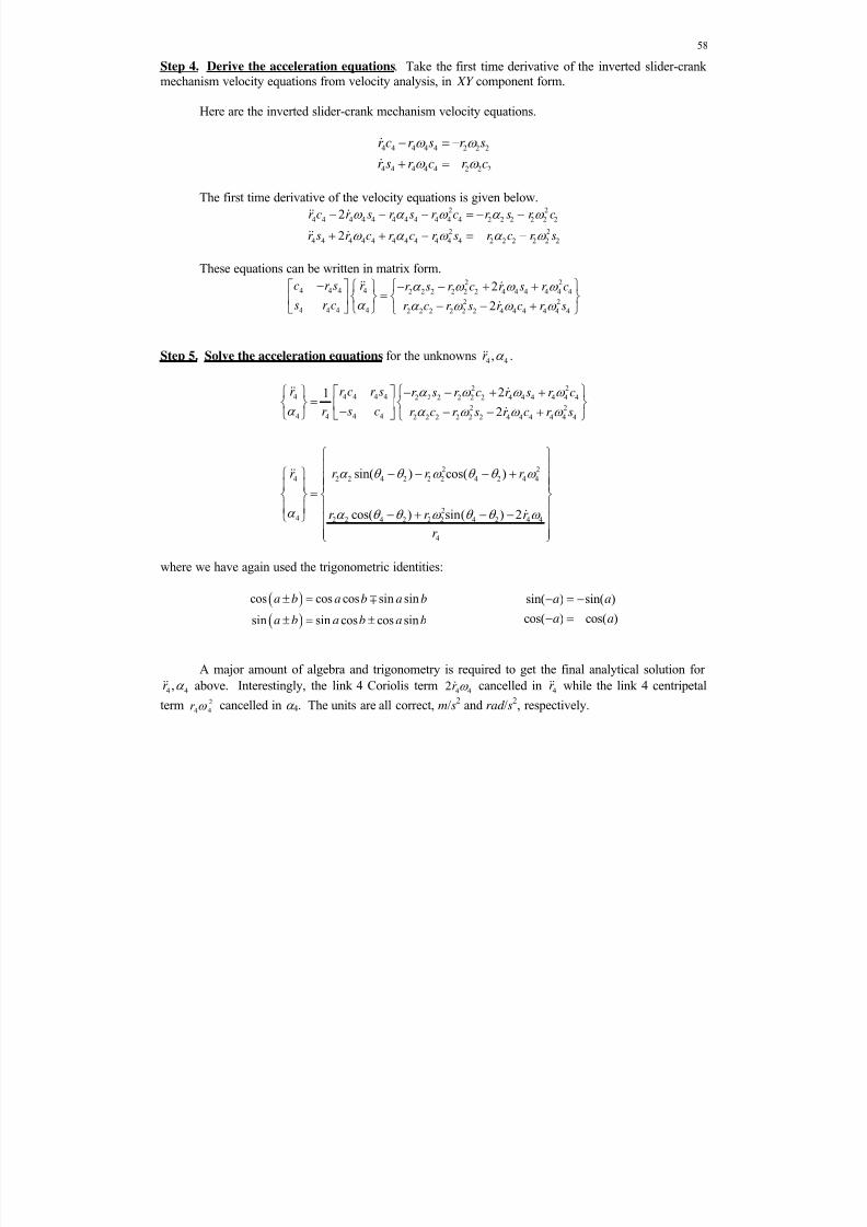
8/11/2019 Mechanism kinematics & dynamics.pdf
http://slidepdf.com/reader/full/mechanism-kinematics-dynamicspdf 58/269
58
Step 4. Derive the acceleration equations. Take the first time derivative of the inverted slider-crankmechanism velocity equations from velocity analysis, in XY component form.
Here are the inverted slider-crank mechanism velocity equations.
4 4 4 4 4 2 2 2
4 4 4 4 4 2 2 2
r c r s r s
r s r c r c
The first time derivative of the velocity equations is given below.2 2
4 4 4 4 4 4 4 4 4 4 4 2 2 2 2 2 2
2 2
4 4 4 4 4 4 4 4 4 4 4 2 2 2 2 2 2
2
2
r c r s r s r c r s r c
r s r c r c r s r c r s
These equations can be written in matrix form.2 2
4 4 4 4 2 2 2 2 2 2 4 4 4 4 4 4
2 24 4 4 4 2 2 2 2 2 2 4 4 4 4 4 4
2
2
c r s r r s r c r s r c
s r c r c r s r c r s
Step 5. Solve the acceleration equations for the unknowns 4 4,r .
2 24 4 4 4 4 2 2 2 2 2 2 4 4 4 4 4 4
2 24 4 44 2 2 2 2 2 2 4 4 4 4 4 4
2 2
4 2 2 4 2 2 2 4 2 4 4
24 2 2 4 2 2 2 4 2 4 4
4
21
2
sin( ) cos( )
cos( ) sin( ) 2
r r c r s r s r c r s r c
s cr r c r s r c r s
r r r r
r r r
r
where we have again used the trigonometric identities:
cos cos cos sin sin
sin sin cos cos sin
a b a b a b
a b a b a b
sin( ) sin( )
cos( ) cos( )
a a
a a
A major amount of algebra and trigonometry is required to get the final analytical solution for
4 4,r above. Interestingly, the link 4 Coriolis term4 42r cancelled in 4
r while the link 4 centripetal
term 2
4 4r cancelled in 4. The units are all correct, m/s2 and rad /s2, respectively.
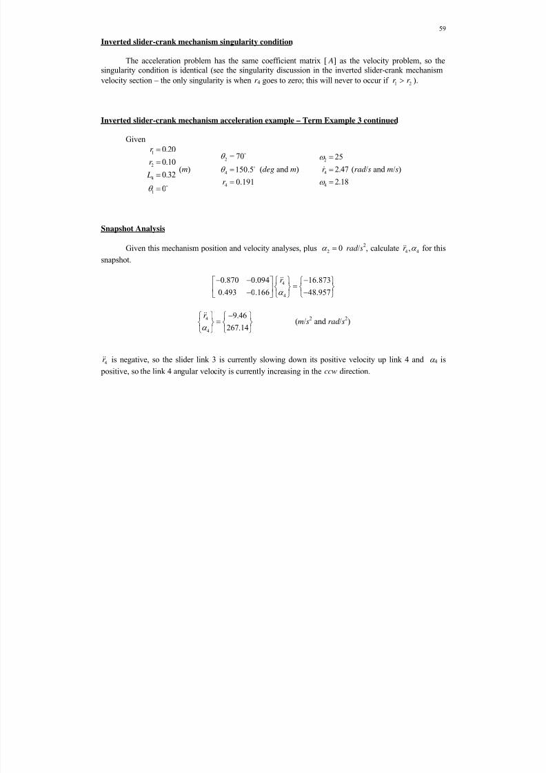
8/11/2019 Mechanism kinematics & dynamics.pdf
http://slidepdf.com/reader/full/mechanism-kinematics-dynamicspdf 59/269
59
Inverted slider-crank mechanism singularity condition
The acceleration problem has the same coefficient matrix [ A] as the velocity problem, so thesingularity condition is identical (see the singularity discussion in the inverted slider-crank mechanism
velocity section – the only singularity is when r 4 goes to zero; this will never to occur if 1 2r r ).
Inverted slider-crank mechanism acceleration example – Term Example 3 continued
Given
1
2
4
1
0.20
0.10
0.32
0
r
r
L
(m)
2
4
4
70
150.5
0.191r
(deg and m)
2
4
4
25
2.47
2.18
r
(rad /s and m/s)
Snapshot Analysis
Given this mechanism position and velocity analyses, plus 2 0 rad /s2, calculate 4 4,r for this
snapshot.
4
4
0.870 0.094 16.873
0.493 0.166 48.957
r
4
4
9.46
267.14
r
(m/s2 and rad /s2)
4r is negative, so the slider link 3 is currently slowing down its positive velocity up link 4 and 4 is
positive, so the link 4 angular velocity is currently increasing in the ccw direction.
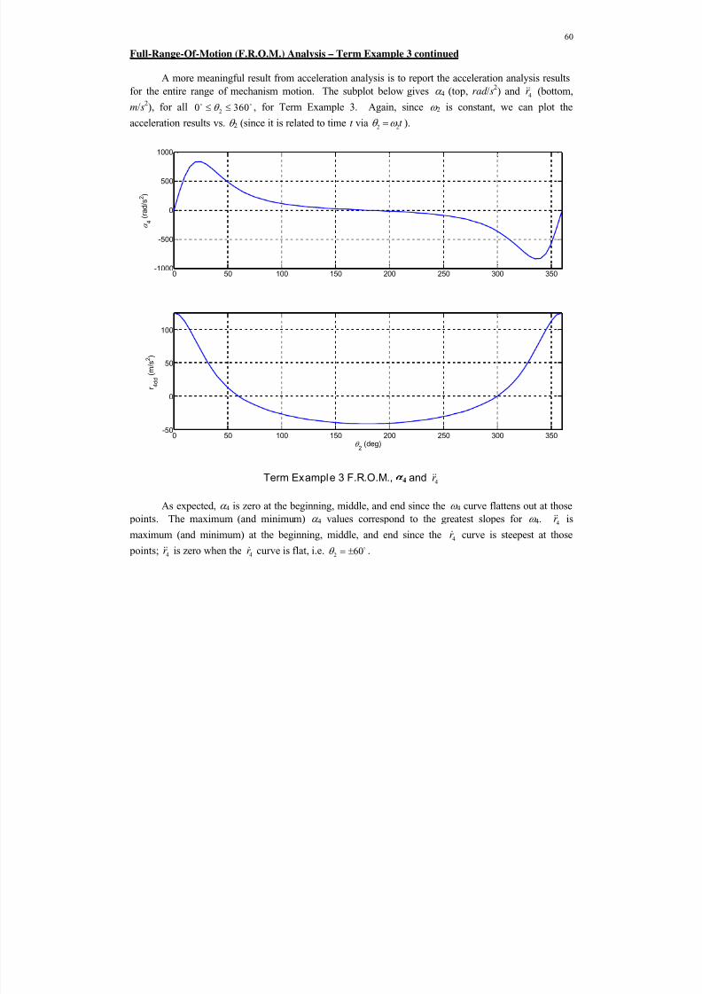
8/11/2019 Mechanism kinematics & dynamics.pdf
http://slidepdf.com/reader/full/mechanism-kinematics-dynamicspdf 60/269
60
Full-Range-Of-Motion (F.R.O.M.) Analysis – Term Example 3 continued
A more meaningful result from acceleration analysis is to report the acceleration analysis results
for the entire range of mechanism motion. The subplot below gives 4 (top, rad /s2) and 4
r (bottom,
m/s2), for all20 360 , for Term Example 3. Again, since 2 is constant, we can plot the
acceleration results vs. 2 (since it is related to time t via 2 2t ).
Term Example 3 F.R.O.M., 4 and 4r
As expected, 4 is zero at the beginning, middle, and end since the 4 curve flattens out at those
points. The maximum (and minimum) 4 values correspond to the greatest slopes for 4. 4r is
maximum (and minimum) at the beginning, middle, and end since the 4r curve is steepest at those points; 4r is zero when the 4r curve is flat, i.e.
2 60 .
0 50 100 150 200 250 300 350-1000
-500
0
500
1000
4
( r a d / s
2 )
0 50 100 150 200 250 300 350-50
0
50
100
2 (deg)
r 4 d d
( m / s
2 )

8/11/2019 Mechanism kinematics & dynamics.pdf
http://slidepdf.com/reader/full/mechanism-kinematics-dynamicspdf 61/269
61
Derivative/Integral Relationships
When one variable is the derivative of another, recall the relationships from calculus (thederivative is the slope of the above curve at each point; the integral is the area under the curve up to that point, taking into account the initial value). For example:
44
( )( )
d t t dt
4 40 4( ) ( )t t dt
44
( )( )
d t t
dt
4 40 4( ) ( )t t dt
0 50 100 150 200 250 300 350
160
180
200
4
( d e g )
0 50 100 150 200 250 300 350
-20
-10
0
10
4
( r a d / s )
0 50 100 150 200 250 300 350-1000
-500
0
500
1000
2 (deg)
4
( r a d / s 2 )
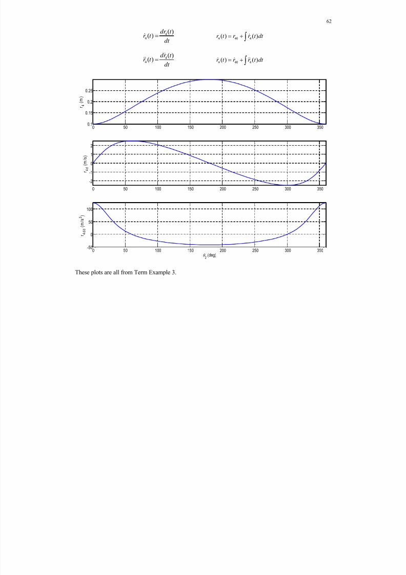
8/11/2019 Mechanism kinematics & dynamics.pdf
http://slidepdf.com/reader/full/mechanism-kinematics-dynamicspdf 62/269
62
44
( )( )
dr t r t
dt 4 40 4( ) ( )r t r r t dt
44
( )( )
dr t r t
dt
4 40 4( ) ( )r t r r t dt
These plots are all from Term Example 3.
0 50 100 150 200 250 300 3500.1
0.15
0.2
0.25
r 4
( m
)
0 50 100 150 200 250 300 350
-2
-1
0
1
2
r 4
d
( m
/ s )
0 50 100 150 200 250 300 350-50
0
50
100
2 (deg)
r 4 d
d
( m
/ s 2 )

8/11/2019 Mechanism kinematics & dynamics.pdf
http://slidepdf.com/reader/full/mechanism-kinematics-dynamicspdf 63/269
63
2.3.6 Multi-Loop Mechanism Acceleration Analysis
Thus far we have presented acceleration analysis for the single-loop four-bar, slider-crank, andinverted slider-crank mechanisms. The acceleration analysis for mechanisms of more than one loop ishandled using the same general procedures developed for the single loop mechanisms.
This section presents acceleration analysis for the two-loop Stephenson I six-bar mechanismshown below as an example multi-loop mechanism. It follows the position and velocity analyses for thesame mechanism presented earlier.
Stephenson I 6-Bar Mechanism
The bottom loop of the Stephenson I six-bar mechanism is identical to the standard four-bar
mechanism model and so the acceleration analysis solution is identical to the four-bar presented earlier.With the complete acceleration analysis of the bottom loop thus solved, the solution for the top loop isessentially another four-bar acceleration solution.
As in all acceleration analysis, the acceleration solution for multi-loop mechanisms is a linearanalysis yielding a unique solution (assuming the given mechanism position is not singular) for eachsolution branch considered. The position and velocity analyses must be complete prior to theacceleration solution.
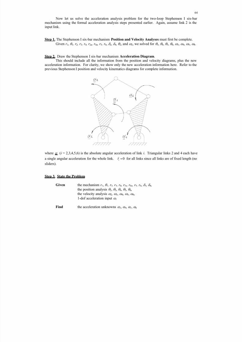
8/11/2019 Mechanism kinematics & dynamics.pdf
http://slidepdf.com/reader/full/mechanism-kinematics-dynamicspdf 64/269
64
Now let us solve the acceleration analysis problem for the two-loop Stephenson I six-barmechanism using the formal acceleration analysis steps presented earlier. Again, assume link 2 is theinput link.
Step 1. The Stephenson I six-bar mechanism Position and Velocity Analyses must first be complete.
Given r 1, 1 , r 2 , r 3 , r 4 , r 2a , r 4a , r 5 , r 6, 2, 4, 2, and 2, we solved for 3, 4, 5, 6, 3, 4, 5, 6.
Step 2. Draw the Stephenson I six-bar mechanism Acceleration Diagram.This should include all the information from the position and velocity diagrams, plus the new
acceleration information. For clarity, we show only the new acceleration information here. Refer to the previous Stephenson I position and velocity kinematics diagrams for complete information.
where i (i = 2,3,4,5,6) is the absolute angular acceleration of link i. Triangular links 2 and 4 each have
a single angular acceleration for the whole link. 0ir for all links since all links are of fixed length (no
sliders).
Step 3. State the Problem
Given the mechanism r 1, 1 , r 2 , r 3 , r 4 , r 2a , r 4a , r 5 , r 6, 2, 4,the position analysis 2, 3, 4, 5, 6,
the velocity analysis 2, 3, 4, 5, 6,
1-dof acceleration input 2
Find the acceleration unknowns 3, 4, 5, 6
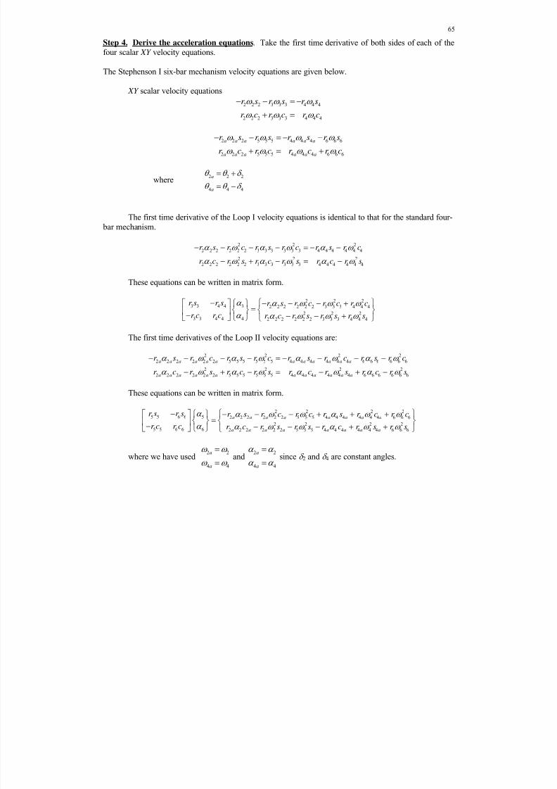
8/11/2019 Mechanism kinematics & dynamics.pdf
http://slidepdf.com/reader/full/mechanism-kinematics-dynamicspdf 65/269
65
Step 4. Derive the acceleration equations. Take the first time derivative of both sides of each of thefour scalar XY velocity equations.
The Stephenson I six-bar mechanism velocity equations are given below.
XY scalar velocity equations
2 2 2 3 3 3 4 4 4
2 2 2 3 3 3 4 4 4
r s r s r s
r c r c r c
2 2 2 5 5 5 4 4 4 6 6 6
2 2 2 5 5 5 4 4 4 6 6 6
a a a a a a
a a a a a a
r s r s r s r s
r c r c r c r c
where2 2 2
4 4 4
a
a
The first time derivative of the Loop I velocity equations is identical to that for the standard four- bar mechanism.
2 2 2
2 2 2 2 2 2 3 3 3 3 3 3 4 4 4 4 4 4
2 2 2
2 2 2 2 2 2 3 3 3 3 3 3 4 4 4 4 4 4
r s r c r s r c r s r c
r c r s r c r s r c r s
These equations can be written in matrix form.
2 2 23 3 4 4 3 2 2 2 2 2 2 3 3 3 4 4 4
2 2 2
3 3 4 4 4 2 2 2 2 2 2 3 3 3 4 4 4
r s r s r s r c r c r c
r c r c r c r s r s r s
The first time derivatives of the Loop II velocity equations are:
2 2 2 2
2 2 2 2 2 2 5 5 5 5 5 5 4 4 4 4 4 4 6 6 6 6 6 6
2 2 2 2
2 2 2 2 2 2 5 5 5 5 5 5 4 4 4 4 4 4 6 6 6 6 6 6
a a a a a a a a a a a a
a a a a a a a a a a a a
r s r c r s r c r s r c r s r c
r c r s r c r s r c r s r c r s
These equations can be written in matrix form.
2 2 2 25 5 6 6 5 2 2 2 2 2 2 5 5 5 4 4 4 4 4 4 6 6 6
2 2 2 25 5 6 6 6 2 2 2 2 2 2 5 5 5 4 4 4 4 4 4 6 6 6
a a a a a a a a
a a a a a a a a
r s r s r s r c r c r s r c r c
r c r c r c r s r s r c r s r s
where we have used2 2
4 4
a
a
and
2 2
4 4
a
a
since 2 and 4 are constant angles.
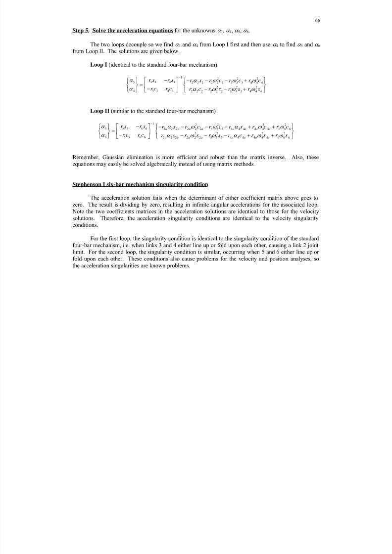
8/11/2019 Mechanism kinematics & dynamics.pdf
http://slidepdf.com/reader/full/mechanism-kinematics-dynamicspdf 66/269
66
Step 5. Solve the acceleration equations for the unknowns 3, 4, 5, 6.
The two loops decouple so we find 3 and 4 from Loop I first and then use 4 to find 5 and 6 from Loop II. The solutions are given below.
Loop I (identical to the standard four-bar mechanism)
1 2 2 23 3 4 43 2 2 2 2 2 2 3 3 3 4 4 4
2 2 23 3 4 44 2 2 2 2 2 2 3 3 3 4 4 4
r s r s r s r c r c r c
r c r c r c r s r s r s
Loop II (similar to the standard four-bar mechanism)
1 2 2 2 25 5 5 6 6 2 2 2 2 2 2 5 5 5 4 4 4 4 4 4 6 6 6
2 2 2 26 5 5 6 6 2 2 2 2 2 2 5 5 5 4 4 4 4 4 4 6 6 6
a a a a a a a a
a a a a a a a a
r s r s r s r c r c r s r c r c
r c r c r c r s r s r c r s r s
Remember, Gaussian elimination is more efficient and robust than the matrix inverse. Also, theseequations may easily be solved algebraically instead of using matrix methods.
Stephenson I six-bar mechanism singularity condition
The acceleration solution fails when the determinant of either coefficient matrix above goes tozero. The result is dividing by zero, resulting in infinite angular accelerations for the associated loop. Note the two coefficients matrices in the acceleration solutions are identical to those for the velocitysolutions. Therefore, the acceleration singularity conditions are identical to the velocity singularity
conditions.
For the first loop, the singularity condition is identical to the singularity condition of the standardfour-bar mechanism, i.e. when links 3 and 4 either line up or fold upon each other, causing a link 2 jointlimit. For the second loop, the singularity condition is similar, occurring when 5 and 6 either line up orfold upon each other. These conditions also cause problems for the velocity and position analyses, sothe acceleration singularities are known problems.

8/11/2019 Mechanism kinematics & dynamics.pdf
http://slidepdf.com/reader/full/mechanism-kinematics-dynamicspdf 67/269
67
2.4 Other Kinematics Topics
2.4.1 Link Extensions Graphics
Using the methods presented thus far, we can use MATLAB to animate mechanisms for theentire range of motion. However, these methods have focused on the basic models shown below. Whatif your term project requires animation of modifications of these basic mechanisms with extensions fromthe existing rigid links?
Four-Bar Mechanism Offset Slider-Crank Mechanism
Four-bar mechanism link 3 extensions
Here are the kinematics equations (we already presented the point C kinematics equations in the ME3011 NotesBook).
3 3
3 3
cos( )
sin( )
x x CA C
y y CA C
c a r
c a r
C 3 3
3 3
cos( )
sin( )
x x DB D
y y DB D
d b r
d b r
D
where2 2
2 2
cos
sin
x
y
a r
a r
A
1 1 4 4
1 1 4 4
cos cos
sin sin
x
y
b r r
b r r
B
In this simple straight-line case, use3 180C
and3 0 D
. Here is partial MATLAB code for link 3
extensions animation.x2 = [0 ax(i)]; % coordinates of link 2 y2 = [0 ay(i)];x3 = [cx(i) dx(i)]; % coordinates of link 3 y3 = [cy(i) dy(i)];x4 = [r1x bx(i)]; % coordinates of link 4 y4 = [r1y by(i)];figure; plot(x2,y2,'r',x3,y3,'g',x4,y4,'b');
C
D
A
B

8/11/2019 Mechanism kinematics & dynamics.pdf
http://slidepdf.com/reader/full/mechanism-kinematics-dynamicspdf 68/269
68
Four-bar mechanism link 4 extensions
The kinematics equations are given below.
4 4
4 4
cos( )
sin( )
x x CB C
y y CB C
c b r
c b r
C 4
4
4 4 4
4 4 4
cos( )
sin( )
x DO D x
y y DO D
O r d
d O r
D
In this simple straight-line case, use4 0C
and4 180 D
. b x and b y were given above and4
O is:
1 1
1 1
cos
sin
r
r
4O
Here is partial MATLAB code for link 4 extensions animation.x2 = [0 ax(i)]; % coordinates of link 2 y2 = [0 ay(i)];x3 = [ax(i) bx(i)]; % coordinates of link 3 y3 = [ay(i) by(i)];x4 = [cx(i) dx(i)]; % coordinates of link 4
y4 = [cy(i) dy(i)];figure; plot(x2,y2,'r',x3,y3,'g',x4,y4,'b');
Of course, one can use combinations of these graphics approaches as necessary. Also, use patch for drawing solid polygonal links rather than straight lines. You can also use patch for
drawing solid circles. This method is also extendable to non-straight-line links by using the appropriate
angles.
C
D
A
B
O4

8/11/2019 Mechanism kinematics & dynamics.pdf
http://slidepdf.com/reader/full/mechanism-kinematics-dynamicspdf 69/269
69
2.5 Jerk Kinematics Analysis
Jerk is the time rate of change of the acceleration (and hence the second and third time rates ofchange of the velocity and position, respectively). Again, this jerk time rate of change may describe achange in magnitude of acceleration, a change in direction of acceleration, or both. What names have been given to the next three position derivatives after jerk? The answer is given somewhere in thissection. Jerk analysis is the fourth step in kinematics analysis. It is not required for standard Newton-Euler dynamics analysis. However, it is useful for the following items.
Input link motion specification
Cam motion profiles and cam design
Smooth motion control as in elevators
Jerk can be important for kinematic motion analysis in general. Position, velocity, andacceleration analyses must be completed first. Jerk is the first time derivative of the acceleration, thesecond time derivative of the velocity, and the third time derivative of the position. Like all the terms preceding it, jerk is also a vector quantity. There are both translational and rotational jerk terms.
2 3
2 3
( ) ( ) ( )( )
d A t d V t d P t J t
dt dt dt SI units: 3
m
s
2 3
2 3
( ) ( ) ( )( )
d t d t d t t
dt dt dt
SI units: 3
rad
s
2.5.1 Jerk Analysis Introduction
In this section we will derive the n-part jerk formula, showing the most general jerk terms possible for planar devices.
n-part Jerk Derivation Figure
This is a four-dof system consisting of a translating/rotating rigid rod with a slider. The samesystem was used for the two-part position, three-part velocity, and five-part accelerations formuladerivations in the ME 3011 NotesBook. Find the total jerk of the point P, which is on the slider.
Y
L
X
L, L, L
P
O
PO

8/11/2019 Mechanism kinematics & dynamics.pdf
http://slidepdf.com/reader/full/mechanism-kinematics-dynamicspdf 70/269
70
Start with the five-part acceleration formula from before and take another time derivate of the XY components. What is n? (Hint – clearly n must be greater than 5.)
2
2
cos 2 sin sin cos
sin 2 cos cos sin
OX PP
OY
A A V L Ld A d J
dt dt A A V L L
Recall the two-part position, three-part velocity, and five-part acceleration formula results below.
2
2
cos
sin
cos sin
sin cos
2
cos 2 sin sin cos
sin 2 cos cos sin
P O
OX
OY
P O
OX
OY
P O
OX
OY
P P L
P L
P L
V V V L
V V L
V V L
A A A V L L
A A V L L
A A V L L
The angle , angular velocity , angular acceleration , and angular jerk are all changing with respectto time (only the planar case is this simple; the spatial rotation case is more complicated).
2 3
2 3
d d d
dt dt dt
The rod length L, sliding velocity V , sliding acceleration A, and sliding jerk J are all changing withrespect to time.
2 3
2 3
d A d V d L J
dt dt dt
Here are the same relationships, using the dot notation to indicate time differentiation.
2 3
2 3
d d d
dt dt dt
2 3
2 3
d L d L d L L
dt dt dt
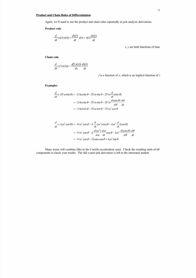
8/11/2019 Mechanism kinematics & dynamics.pdf
http://slidepdf.com/reader/full/mechanism-kinematics-dynamicspdf 71/269
71
Product and Chain Rules of Differentiation
Again, we’ll need to use the product and chain rules repeatedly in jerk analysis derivations.
Product rule
( ) ( )( ( ) ( )) ( ) ( )
d dx t dy t x t y t y t x t dt dt dt
x, y are both functions of time
Chain rule
( ( )) ( )( ( ( )))
d df x t dx t f x t
dt dx dt
f is a function of x, which is an implicit function of t
Examples
2
( 2 sin ) 2 sin 2 sin 2 (sin )
(sin )2 sin 2 sin 2
2 sin 2 sin 2 cos
d d V A V V
dt dt
d d A V V
d dt
A V V
2 2 2 2
22 2
2 3
( cos ) cos ( )cos (cos )
( ) (cos )cos cos
cos 2 cos sin
d d d L V L L
dt dt dt
d d d d V L L
d dt d dt
V L L
Many terms will combine (like in the Coriolis acceleration case). Check the resulting units of allcomponents to check your results. The full n-part jerk derivation is left to the interested student.

8/11/2019 Mechanism kinematics & dynamics.pdf
http://slidepdf.com/reader/full/mechanism-kinematics-dynamicspdf 72/269
72
2.5.2 Mechanism Jerk Analys is
Generic Mechanism Jerk Analysis Problem Statement
Given the mechanism, complete position, velocity, and acceleration analyses, and one-dof of jerkinput, calculate the jerk unknowns.
For a given branch of a known mechanism, this will yield linear equations so a matrix-vectorapproach may be used to obtain the unique solution (assuming no singularity).
Since jerk kinematics is not required for dynamics analysis or machine design (generally), thissolution is beyond the scope of the class.
For our jerk needs, we may use the time differentiation approach of the previous subsection.
Snap, what a happy soundSnap is the happiest sound I found
You may clap, rap, tap, slap,But Snap makes the world go roundSnap, crackle, pop – Rice Krispies!
I say it’s Crackle, the crispy soundYou gotta have Crackle or the clock’s not wound
Geese cackle, feathers tickle, belts buckle, beets pickle,But Crackle makes the world go round
Snap, crackle, pop – Rice Krispies!
I insist that Pop’s the soundThe best is missed unless Pop’s around
You can’t stop hoppin’ when the cereal’s poppin’Pop makes the world go round
Snap, crackle, pop – Rice Krispies!
-Old Kellogg’s Advertisement
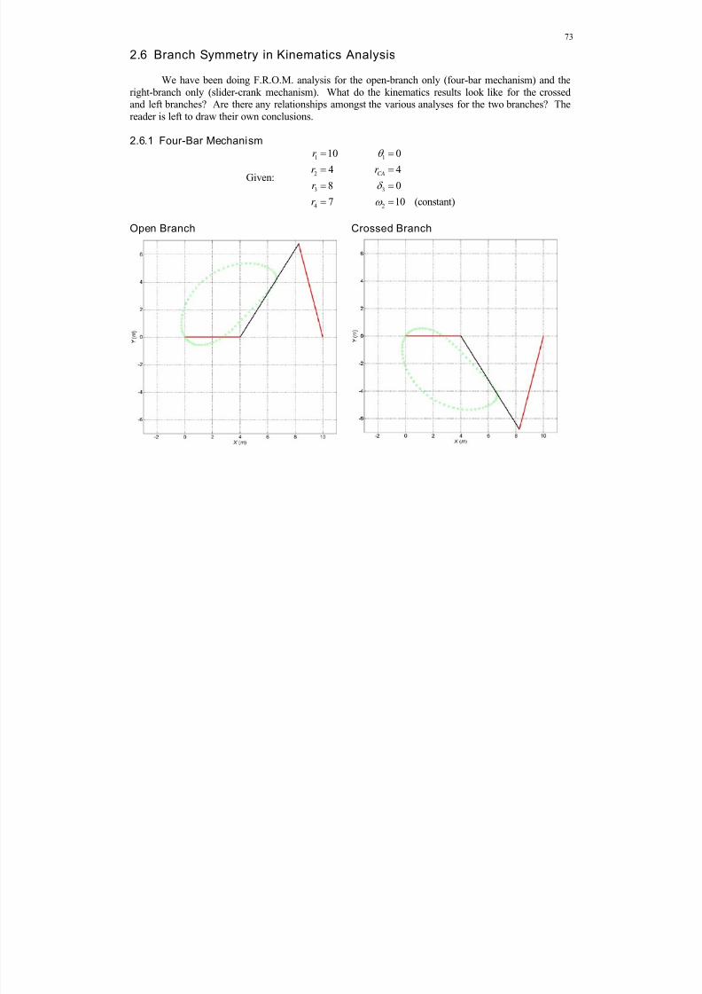
8/11/2019 Mechanism kinematics & dynamics.pdf
http://slidepdf.com/reader/full/mechanism-kinematics-dynamicspdf 73/269
73
2.6 Branch Symmetry in Kinematics Analysis
We have been doing F.R.O.M. analysis for the open-branch only (four-bar mechanism) and theright-branch only (slider-crank mechanism). What do the kinematics results look like for the crossedand left branches? Are there any relationships amongst the various analyses for the two branches? Thereader is left to draw their own conclusions.
2.6.1 Four-Bar Mechanism
Given:
1
2
3
4
10
4
8
7
r
r
r
r
1
3
2
0
4
0
10 (constant)
CAr
Open Branch Crossed Branch
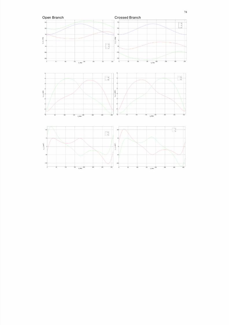
8/11/2019 Mechanism kinematics & dynamics.pdf
http://slidepdf.com/reader/full/mechanism-kinematics-dynamicspdf 74/269
74
Open Branch Crossed Branch
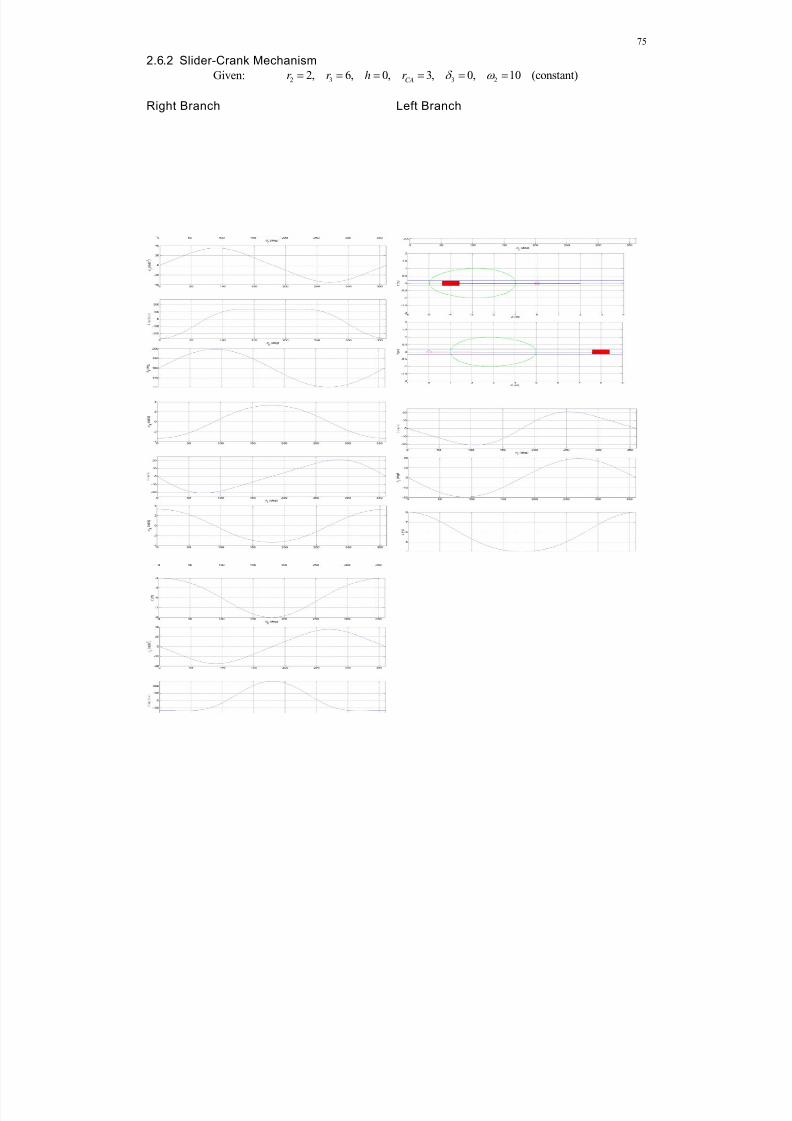
8/11/2019 Mechanism kinematics & dynamics.pdf
http://slidepdf.com/reader/full/mechanism-kinematics-dynamicspdf 75/269
75
2.6.2 Slider-Crank Mechanism
Given: 2 3 3 22, 6, 0, 3, 0, 10 (constant)CA
r r h r
Right Branch Left Branch

8/11/2019 Mechanism kinematics & dynamics.pdf
http://slidepdf.com/reader/full/mechanism-kinematics-dynamicspdf 76/269
76
We see a great deal of symmetry for both four-bar and slider crank mechanism kinematic
analyses. The coupler point curves and all plots have either horizontal midpoint 2 180 or vertical
zero point flip-symmetry (some have both).
However, for the x and x slider-crank mechanism results, this symmetry is not immediately
evident. This special symmetry is revealed when first cutting the plots at 2 180 , and then performing
the horizontal and/or vertical flipping.
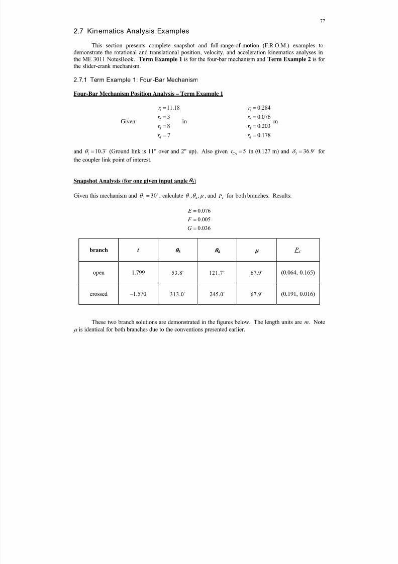
8/11/2019 Mechanism kinematics & dynamics.pdf
http://slidepdf.com/reader/full/mechanism-kinematics-dynamicspdf 77/269
77
2.7 Kinematics Analysis Examples
This section presents complete snapshot and full-range-of-motion (F.R.O.M.) examples todemonstrate the rotational and translational position, velocity, and acceleration kinematics analyses inthe ME 3011 NotesBook. Term Example 1 is for the four-bar mechanism and Term Example 2 is forthe slider-crank mechanism.
2.7.1 Term Example 1: Four-Bar Mechanism
Four-Bar Mechanism Position Analysis – Term Example 1
Given:
1
2
3
4
11.18
3
8
7
r
r
r
r
in
1
2
3
4
0.284
0.076
0.203
0.178
r
r
r
r
m
and 1 10.3
(Ground link is 11" over and 2" up). Also given 5CAr in (0.127 m) and 3 36.9
forthe coupler link point of interest.
Snapshot Analysis (for one given input angle2)
Given this mechanism and 230 , calculate 3 4, , , and
C P for both branches. Results:
0.076
0.005
0.036
E
F
G
branch t3 4 C P
open 1.799 53.8 121.7 67.9 (0.064, 0.165)
crossed –1.570 313.0 245.0 67.9 (0.191, 0.016)
These two branch solutions are demonstrated in the figures below. The length units are m. Note
is identical for both branches due to the conventions presented earlier.

8/11/2019 Mechanism kinematics & dynamics.pdf
http://slidepdf.com/reader/full/mechanism-kinematics-dynamicspdf 78/269
78
Open Branch (t(2))
Crossed Branch (t(1))
Term Example 1 Snapshot
-0.1 0 0.1 0.2 0.3
-0.1
-0.05
0
0.05
0.1
0.15
0.2
0.25
X (m)
Y ( m )
-0.1 0 0.1 0.2 0.3
-0.1
-0.05
0
0.05
0.1
0.15
0.2
0.25
X (m)
Y ( m )
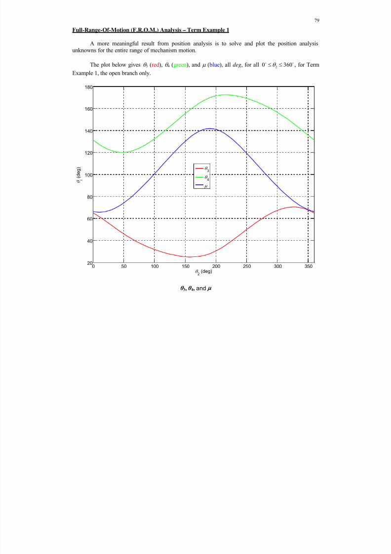
8/11/2019 Mechanism kinematics & dynamics.pdf
http://slidepdf.com/reader/full/mechanism-kinematics-dynamicspdf 79/269
79
Full-Range-Of-Motion (F.R.O.M.) Analysis – Term Example 1
A more meaningful result from position analysis is to solve and plot the position analysisunknowns for the entire range of mechanism motion.
The plot below gives 3 (red ), 4 (green), and ( blue), all deg, for all 20 360 , for Term
Example 1, the open branch only.
3, 4, and
0 50 100 150 200 250 300 35020
40
60
80
100
120
140
160
180
2 (deg)
i
( d e g )
3
4

8/11/2019 Mechanism kinematics & dynamics.pdf
http://slidepdf.com/reader/full/mechanism-kinematics-dynamicspdf 80/269
80
The plot below gives the initial (and final) animation position, for 20,360 . It also gives the
coupler curve for the open branch, plotting PCY vs. PCX in green circles.
C P
Coupler Curve
Term Example 1 F.R.O.M. Posi tion Results
-0.1 -0.05 0 0.05 0.1 0.15 0.2 0.25 0.3
-0.1
-0.05
0
0.05
0.1
0.15
0.2
0.25
X (m)
Y ( m )
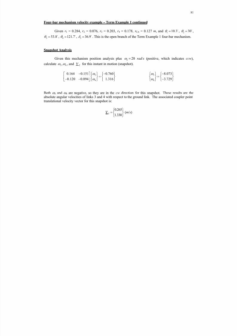
8/11/2019 Mechanism kinematics & dynamics.pdf
http://slidepdf.com/reader/full/mechanism-kinematics-dynamicspdf 81/269
81
Four-bar mechanism velocity example – Term Example 1 continued
Given r 1 = 0.284, r 2 = 0.076, r 3 = 0.203, r 4 = 0.178, r C A = 0.127 m, and 110.3 , 2
30 ,
353.8 , 4
121.7 , 336.9 . This is the open branch of the Term Example 1 four-bar mechanism.
Snapshot Analysis
Given this mechanism position analysis plus 2 20 rad /s (positive, which indicates ccw),
calculate 3 4, , and C V for this instant in motion (snapshot).
3
4
0.164 0.151 0.760
0.120 0.094 1.316
3
4
8.073
3.729
Both 3 and 4 are negative, so they are in the cw direction for this snapshot. These results are theabsolute angular velocities of links 3 and 4 with respect to the ground link. The associated coupler pointtranslational velocity vector for this snapshot is:
0.265
1.330C V
(m/s)
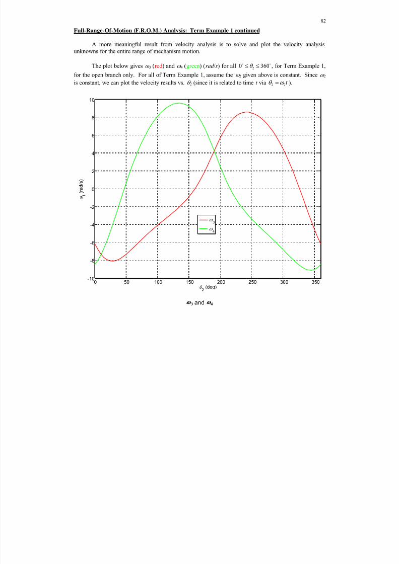
8/11/2019 Mechanism kinematics & dynamics.pdf
http://slidepdf.com/reader/full/mechanism-kinematics-dynamicspdf 82/269
82
Full-Range-Of-Motion (F.R.O.M.) Analysis: Term Example 1 continued
A more meaningful result from velocity analysis is to solve and plot the velocity analysisunknowns for the entire range of mechanism motion.
The plot below gives 3 (red ) and 4 (green) (rad /s) for all 20 360 , for Term Example 1,
for the open branch only. For all of Term Example 1, assume the 2 given above is constant. Since 2 is constant, we can plot the velocity results vs. 2 (since it is related to time t via 2 2t ).
3 and 4
0 50 100 150 200 250 300 350-10
-8
-6
-4
-2
0
2
4
6
8
10
2 (deg)
i
( r a d / s )
3
4

8/11/2019 Mechanism kinematics & dynamics.pdf
http://slidepdf.com/reader/full/mechanism-kinematics-dynamicspdf 83/269
83
The plot below gives the absolute translational coupler point C velocity for all 20 360 , for
Term Example 1, for the open branch only.
C V
Term Example 1 F.R.O.M. Velocity Results
0 50 100 150 200 250 300 350-1.5
-1
-0.5
0
0.5
1
1.5
2
2 (deg)
V C
( m / s )
VCX
VCY

8/11/2019 Mechanism kinematics & dynamics.pdf
http://slidepdf.com/reader/full/mechanism-kinematics-dynamicspdf 84/269

8/11/2019 Mechanism kinematics & dynamics.pdf
http://slidepdf.com/reader/full/mechanism-kinematics-dynamicspdf 85/269
85
Full-Range-Of-Motion (F.R.O.M.) Analysis – Term Example 1 continued
A more meaningful result from acceleration analysis is to solve and plot the acceleration analysisunknowns for the entire range of mechanism motion.
The plot below gives 3 (red ) and 4 (green), (rad /s2), for all 20 360 , for Term Example
1, open branch. In the Term Example 1 velocity section it was assumed that the given 2 is constant,which means that the given 2 is always zero. Since 2 is constant, we can plot the acceleration results
vs. 2 (since it is related to time t via 2 2t ).
3 and 4
0 50 100 150 200 250 300 350-250
-200
-150
-100
-50
0
50
100
150
200
250
2 (deg)
i
( r a d / s
2 )
3
4

8/11/2019 Mechanism kinematics & dynamics.pdf
http://slidepdf.com/reader/full/mechanism-kinematics-dynamicspdf 86/269
86
The plot below gives the translational coupler point acceleration for all 20 360 , for Term
Example 1, the open branch only.
C A
Term Example 1 F.R.O.M. Acceleration Results
0 50 100 150 200 250 300 350
-30
-20
-10
0
10
20
30
2 (deg)
A C
( m / s 2 )
ACX
ACY
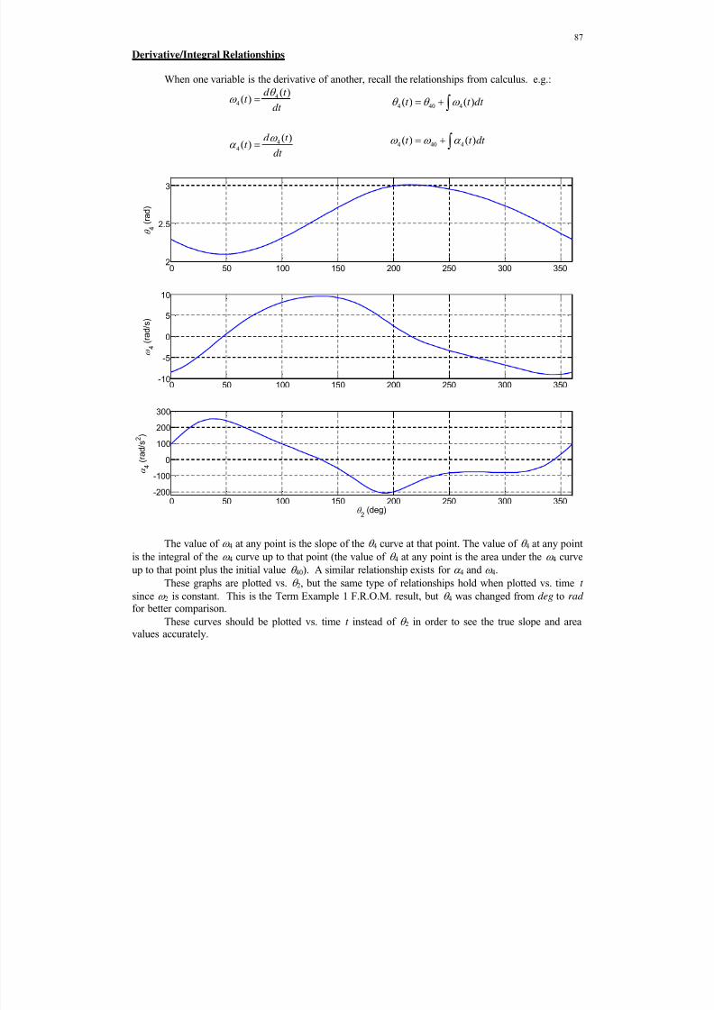
8/11/2019 Mechanism kinematics & dynamics.pdf
http://slidepdf.com/reader/full/mechanism-kinematics-dynamicspdf 87/269
87
Derivative/Integral Relationships
When one variable is the derivative of another, recall the relationships from calculus. e.g.:
44
44
( )( )
( )( )
d t t
dt
d t t dt
4 40 4
4 40 4
( ) ( )
( ) ( )
t t dt
t t dt
The value of 4 at any point is the slope of the 4 curve at that point. The value of 4 at any pointis the integral of the 4 curve up to that point (the value of 4 at any point is the area under the 4 curve
up to that point plus the initial value 40). A similar relationship exists for 4 and 4.
These graphs are plotted vs. 2, but the same type of relationships hold when plotted vs. time t
since 2 is constant. This is the Term Example 1 F.R.O.M. result, but 4 was changed from deg to rad for better comparison.
These curves should be plotted vs. time t instead of 2 in order to see the true slope and areavalues accurately.
0 50 100 150 200 250 300 3502
2.5
3
4
( r a d )
0 50 100 150 200 250 300 350-10
-5
0
5
10
4
( r a d / s )
0 50 100 150 200 250 300 350-200
-100
0
100
200
300
4
( r a d / s 2 )
2 (deg)
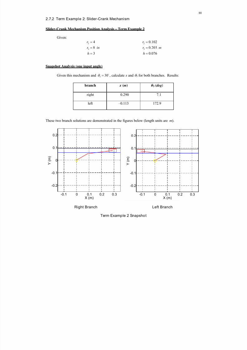
8/11/2019 Mechanism kinematics & dynamics.pdf
http://slidepdf.com/reader/full/mechanism-kinematics-dynamicspdf 88/269
88
2.7.2 Term Example 2: Slider-Crank Mechanism
Slider-Crank Mechanism Position Analysis – Term Example 2
Given:
2
3
4
8
3
r
r
h
in
2
3
0.102
0.203
0.076
r
r
h
m
Snapshot Analysis (one input angle)
Given this mechanism and 230 , calculate x and 3 for both branches. Results:
branch x ( m) 3 ( deg)
right 0.290 7.1
left –0.113 172.9
These two branch solutions are demonstrated in the figures below (length units are m).
Right Branch Left Branch
Term Example 2 Snapshot
-0.1 0 0.1 0.2 0.3
-0.2
-0.1
0
0.1
0.2
X (m)
Y
( m )
-0.1 0 0.1 0.2 0.3
-0.2
-0.1
0
0.1
0.2
X (m)
Y ( m )

8/11/2019 Mechanism kinematics & dynamics.pdf
http://slidepdf.com/reader/full/mechanism-kinematics-dynamicspdf 89/269

8/11/2019 Mechanism kinematics & dynamics.pdf
http://slidepdf.com/reader/full/mechanism-kinematics-dynamicspdf 90/269
90
The plot below gives the initial (and final) animation position, for 20,360 . It also gives the
coupler curve to scale for the right branch, plotting PCY vs. PCX in green. In this case the coupler point istaken to be the midpoint of coupler link 3.
C P Coupler Curve
Term Example 2 F.R.O.M. Posi tion Results
For Term Example 2, the slider translation limits are 0.067 0.295 x , as seen in the x plot
above, calculated from the equations in the 3011 NotesBook.
-0.05 0 0.05 0.1 0.15 0.2 0.25 0.3 0.35-0.2
-0.15
-0.1
-0.05
0
0.05
0.1
0.15
0.2
X (m)
Y ( m )
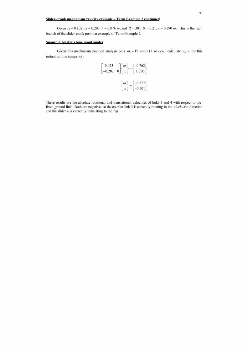
8/11/2019 Mechanism kinematics & dynamics.pdf
http://slidepdf.com/reader/full/mechanism-kinematics-dynamicspdf 91/269
91
Slider-crank mechanism velocity example – Term Example 2 continued
Given r 2 = 0.102, r 3 = 0.203, h = 0.076 m, and 2 30 , 3 7.2 , x = 0.290 m. This is the right
branch of the slider-crank position example of Term Example 2.
Snapshot Analysis (one input angle)
Given this mechanism position analysis plus 2 15 rad /s (+ so ccw), calculate3 , x for this
instant in time (snapshot).
3
3
0.025 1 0.762
0.202 0 1.320
6.577
0.601
x
x
These results are the absolute rotational and translational velocities of links 3 and 4 with respect to thefixed ground link. Both are negative, so the coupler link 3 is currently rotating in the clockwise directionand the slider 4 is currently translating to the left .
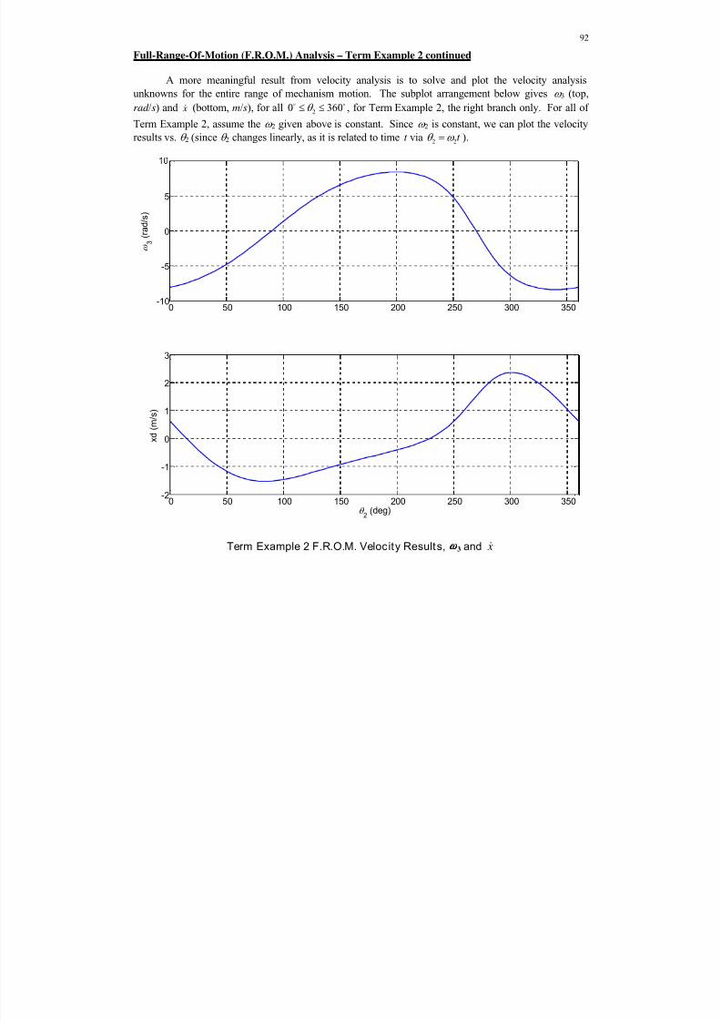
8/11/2019 Mechanism kinematics & dynamics.pdf
http://slidepdf.com/reader/full/mechanism-kinematics-dynamicspdf 92/269
92
Full-Range-Of-Motion (F.R.O.M.) Analysis – Term Example 2 continued
A more meaningful result from velocity analysis is to solve and plot the velocity analysis
unknowns for the entire range of mechanism motion. The subplot arrangement below gives 3 (top,
rad /s) and x (bottom, m/s), for all 20 360 , for Term Example 2, the right branch only. For all of
Term Example 2, assume the 2 given above is constant. Since 2 is constant, we can plot the velocity
results vs. 2 (since 2 changes linearly, as it is related to time t via 2 2t ).
Term Example 2 F.R.O.M. Velocity Results, 3 and x
0 50 100 150 200 250 300 350-10
-5
0
5
3
( r a d / s )
0 50 100 150 200 250 300 350-2
-1
0
1
2
3
2 (deg)
x d ( m / s )

8/11/2019 Mechanism kinematics & dynamics.pdf
http://slidepdf.com/reader/full/mechanism-kinematics-dynamicspdf 93/269
93
Slider-crank mechanism acceleration example – Term Example 2 continued
Given r 2 = 0.102, r 3 = 0.203, h = 0.076 m, and 2 30 , 3 7.2 , x = 0.290 m; and 2 15 ,
3 6.55 rad /s, 0.60 x m/s. This is the right branch of the position and velocity example for the
slider-crank mechanism of Term Example 2.
Snapshot Analysis (one input angle)
Given this mechanism position and velocity analysis plus 2 0 rad /s2, calculate 3 , x for this
snapshot in time.
3
3
0.025 1 28.590
0.202 0 12.557
62.329
30.148
x
x
These results are the absolute angular and linear accelerations of links 3 and 4 with respect to the fixedground link.

8/11/2019 Mechanism kinematics & dynamics.pdf
http://slidepdf.com/reader/full/mechanism-kinematics-dynamicspdf 94/269
94
Full-Range-Of-Motion (F.R.O.M.) Analysis – Term Example 2 continued
A more meaningful result from acceleration analysis is to solve and plot the acceleration analysis
unknowns for the entire range of slider-crank mechanism motion. The top plot gives 3 (rad /s2) and the
bottom plot gives x (m/s2), for all 20 360 , for Term Example 2, for the right branch only. In the
Term Example 2 velocity section it was assumed that the given 2 is constant, which means that the
given 2 is always zero. Since 2 is constant, we can plot the velocity results vs. 2 (since it is related totime t via 2 2t ).
Term Example 2 F.R.O.M. Acceleration Resul ts, 3 and x
0 50 100 150 200 250 300 350-250
-200
-150
-100
-50
0
50
100
150
3
( r a d / s
2 )
0 50 100 150 200 250 300 350-50
0
50
2 (deg)
x d d ( m / s
2 )
8/11/2019 Mechanism kinematics & dynamics.pdf
http://slidepdf.com/reader/full/mechanism-kinematics-dynamicspdf 95/269
95
3. Dynamics Analysis
3.1 Dynamics Introduction
D’Alembert’s Principle
We can convert dynamics problems into statics problems by the inclusion of a vector inertialforce 0 GF mA and a vector inertial moment 0 G M I . Centrifugal force 2
mr , directed away
from the center of rotation, is an example of an inertial force vector. It’s not really a force but a felteffect of an inertia in acceleration. Using D’Alembert’s principle, the right-hand side of the translationaland rotational dynamics equations is subtracted to the other side of the equation. Then the forces andmoments balance to zero as in statics, when the inertial forces are included in the FBD.
We won’t use this method, but it is mentioned for completeness. We would instead to prefer toconsider statics problems as a subset of dynamics problems, with zero accelerations.
0
0
G
O
R mA
R F
0
0
G
O
T r R I
T r R M
Dynamics Humor from xkcd
xkcd.com

8/11/2019 Mechanism kinematics & dynamics.pdf
http://slidepdf.com/reader/full/mechanism-kinematics-dynamicspdf 96/269
96
3.2 Mass, Center of Gravity, and Mass Moment of InertiaThis section presents a thorough review of mass, center of gravity, and mass moment of inertia,
for use in the translational and rotational dynamics equations for each FBD.
GF m A GZ G M I
Newton’s Second Law Euler’s Rotational Dynamics Equation
Newton’s Second Law requires m and CG, Euler’s Rotational Dynamics Equation requires CG and I GZ .
m PCG I GZ
translational mass center of gravityrotational center of gravity mass moment of inertia
Mass
In Newton’s Second LawGF m A , the mass m is the proportionality constant. Mass is
measure of translational inertia – a resistance to change in motion according to Newton’s First Law.
Mass is also a measure of the storage of translational kinetic energy21
2
T KE mv and the units are kg.
Examples for m, CG, I G
System of particles General rigid body
Rectangular rigid body
Mass calculation
System of particles General rigid body
1
N
i
i
m m
body
m dm
Rectangular rigid body
usingm
V , dm dV , so
body body
m dm dV
/ 2 / 2
/ 2 / 2
b h
b hm tdxdy tbh
m V (an obvious result)
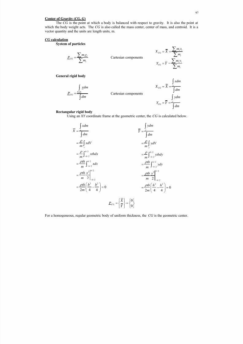
8/11/2019 Mechanism kinematics & dynamics.pdf
http://slidepdf.com/reader/full/mechanism-kinematics-dynamicspdf 97/269
97
Center of Gravity (CG, G) The CG is the point at which a body is balanced with respect to gravity. It is also the point at
which the body weight acts. The CG is also called the mass center, center of mass, and centroid. It is avector quantity and the units are length units, m.
CG calculation
System of particles
ii
CG
i
m r P
m
Cartesian components
i i
CG
i
i i
CG
i
m x X X
m
m yY Y
m
General rigid body
body
CG
rdm
Pdm
Cartesian components
xCG
y
CG
xdm
X X dm
ydm
Y Y dm
Rectangular rigid body Using an XY coordinate frame at the geometric center, the CG is calculated below.
/ 2
/ 2
/ 2
/ 2
/ 22
/ 2
2 2
2
02 4 4
x
x
b
b
b
b
b
b
xdm
X dm
xdV m
xthdxm
th xdx
m
th x
m
th b bm
/ 2
/ 2
/ 2
/ 2
/ 22
/ 2
2 2
2
02 4 4
y
y
h
h
h
h
h
h
ydm
Y dm
ydV m
ytbdym
tb ydy
m
tb y
m
tb h hm
0
0CG
X P
Y
For a homogeneous, regular geometric body of uniform thickness, the CG is the geometric center.
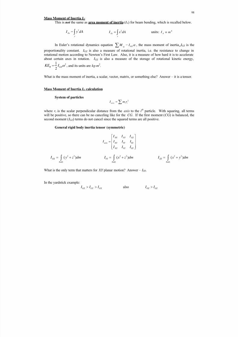
8/11/2019 Mechanism kinematics & dynamics.pdf
http://slidepdf.com/reader/full/mechanism-kinematics-dynamicspdf 98/269
98
Mass Moment of Inertia I G
This is not the same as area moment of inertia ( I A) for beam bending, which is recalled below.
2
Ax
y
I y dA 2
Ay
x
I x dA units: 4
A I m
In Euler’s rotational dynamics equation GZ G M I , the mass moment of inertia I GZ is the proportionality constant. I GZ is also a measure of rotational inertia, i.e. the resistance to change inrotational motion according to Newton’s First Law. Also, it is a measure of how hard it is to accelerateabout certain axes in rotation. I GZ is also a measure of the storage of rotational kinetic energy,
21
2 R GZ
KE I , and its units are kg-m2.
What is the mass moment of inertia, a scalar, vector, matrix, or something else? Answer – it is a tensor.
Mass Moment of Inertia I G calculation
System of particles2
axis i i I m r
where r i is the scalar perpendicular distance from the axis to the ith particle. With squaring, all terms
will be positive, so there can be no canceling like for the CG. If the first moment (CG) is balanced, thesecond moment ( I GZ ) terms do not cancel since the squared terms are all positive.
General rigid body inertia tensor (symmetric)
XX XY XZ
axis XY YY YZ
XZ YZ ZZ
I I I I I I I
I I I
2 2( ) XX
body
I y z dm 2 2( )
YY
body
I x z dm 2 2( )
ZZ
body
I x y dm
What is the only term that matters for XY planar motion? Answer – I ZZ .
In the yardstick example:GZ GY GX
I I I also OZ GZ I I
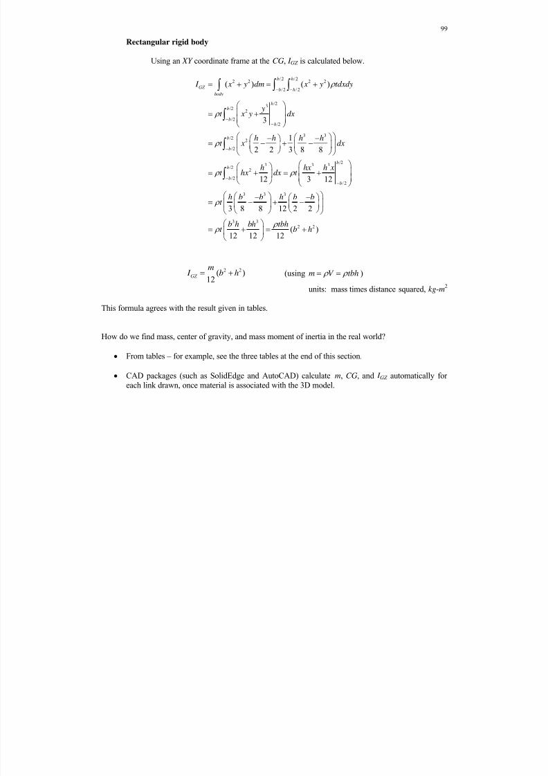
8/11/2019 Mechanism kinematics & dynamics.pdf
http://slidepdf.com/reader/full/mechanism-kinematics-dynamicspdf 99/269
99
Rectangular rigid body
Using an XY coordinate frame at the CG, I GZ is calculated below.
/2 /22 2 2 2
/2 /2
/23/22
/2/2
3 3/2
2
/2
/23 3 3
/22
/2/2
3 3
( ) ( )
3
1
2 2 3 8 8
12 3 12
3 8
b h
GZ b h
body
hb
bh
b
b
bb
bb
I x y dm x y tdxdy
yt x y dx
h h h ht x dx
h hx h xt hx dx t
h b bt
3
3 32 2
8 12 2 2
( )12 12 12
h b b
b h bh tbht b h
2 2( )12
GZ
m I b h (using m V tbh )
units: mass times distance squared, kg-m2
This formula agrees with the result given in tables.
How do we find mass, center of gravity, and mass moment of inertia in the real world?
From tables – for example, see the three tables at the end of this section.
CAD packages (such as SolidEdge and AutoCAD) calculate m, CG, and I GZ automatically foreach link drawn, once material is associated with the 3D model.

8/11/2019 Mechanism kinematics & dynamics.pdf
http://slidepdf.com/reader/full/mechanism-kinematics-dynamicspdf 100/269
100
Parallel Axis Theorem
The mass moment of inertia through the CG is related to mass moments of inertia of parallelaxes through different points as follows.
2
ZZO ZZG I I md
where d is the scalar distance separating the axis of interest O from the axis through the CG. Notice I ZZG
is as small as possible. Any I ZZO must be greater, due to the term md
2
which is always positive.
Parallel axis theorem example
Rectangular rigid body (where axis O is the corner)
2
2 22 2
2 2 2 2
2 2
2 2
( )12 4 4
12 4 12 4
3 3
( )3
ZZO ZZG I I md
m b hb h m
b b h h
m
b hm
mb h
Combining multiple rigid bodies into a rigid link
To combine any number of bodies n of known material, shape, size, and location into one rigid
body, use the following equations for mass, center of gravity, and mass moment of inertia.
1 2
1
n
T n i
i
m m m m m
1 1 2 2 1
1 1 2 2
1
n
i i
n n i
T T T
CGT nn nT
i i
iT
T
m xm x m x m x
m m X P
m y m y m yY m y
m
m
2 2 2 21 1 1 2 2 2
1
n
GZT GZ GZ GZn n n GZi i i
i
I I m d I m d I m d I m d
The subscript ‘T ’ indicates total (or combined) and d i is the distance between the combined CG (T CGP )
and the CG of body i ( i
T
CG i iP x y ). These equations are obtained from the mass, CG, and I GZ
equations for particles, where now each particle is instead a rigid body.

8/11/2019 Mechanism kinematics & dynamics.pdf
http://slidepdf.com/reader/full/mechanism-kinematics-dynamicspdf 101/269
101
Example 1. Two rectangles joined as shown below
Given b1 = 2.2 x h1 = 0.1 x t 1 = 0.005 (m)b2 = 1.0 x h2 = 0.8 x t 2 = 0.005 (m)
the material is steel with a mass density of = 7850 kg/m3
The equations are:
1 2T m m m
1 1 2 2
1 1 2 2
T T
CGT
T
T
m x m x
m X P
m y m yY
m
2 2
1 1 1 2 2 2GZT GZ GZ I I m d I m d
where d i is the distance from CGi to the combined CG CGT P .
The results are:m1 = 8.64 m2 = 31.40 mT = 40.04 (kg)
1
0.05
1.10CGP
2
0.60
1.80CGP
0.48
1.65CGT P
(m)
d 1 = 0.70 d 2 = 0.19 (m)
2 211 1 1 3.49
12GZ
m I b h
2 222 2 2 4.29
12GZ
m I b h I GZT = 13.15 (kgm
2)
Example 1. Two Unequal Steel Rectangles (here b1 is vertical and b2 is horizontal)
0 0.5 1 1.5 20
0.5
1
1.5
2
X (m)
Y ( m )

8/11/2019 Mechanism kinematics & dynamics.pdf
http://slidepdf.com/reader/full/mechanism-kinematics-dynamicspdf 102/269
102
Example 2. Two equal rectangles joined in the same manner
Given b = 2.0 x h = 0.2 x t = 0.005 (m) (twice)
= 7850 kg/m3
The analytical equations for this special case are:
2T
m m 3
4
3
4
T
CGT
T
b h X P
b hY
2 25
( )12
GZT I m b h
where2 2
1 28
b hd d
is the distance from CGi to CGT P .
The results are:m1 = m2 = 15.70 mT = 31.40 (kg)
1
0.10
1.00CGP
2
1.20
1.90CGP
0.65
1.45CGT P
(m)
d 1 = d 2 = 0.71 (m)
2 2
1 2 ( ) 5.2912
GZ GZ
m I I b h I GZT = 26.43 (kgm
2)
Example 2. Two Equal Steel Rectangles(again, b1 is vertical and b2 is horizontal, with b1 = b2 = b here)
0 0.5 1 1.5 20
0.5
1
1.5
2
X (m)
Y ( m )

8/11/2019 Mechanism kinematics & dynamics.pdf
http://slidepdf.com/reader/full/mechanism-kinematics-dynamicspdf 103/269
103
Tables of Mass, Center of Gravity, and Mass Moment of Inertia
The tables below present the mass (kg), center of gravity (m), and mass moment of inertia (kg-m
2) for some common planar link shapes.
Note that mass moment of inertia (kg-m2) is not the same as area moment of inertia for beam bending (m
4). The former represents rotational inertia while the latter is a measure of resistance to beam
bending.
We assume that all link materials are homogeneous and uniformly distributed, with mass density
(kg/m3), all links have regular geometry, and all links have a constant thickness t in the Z direction.
The general equations for mass, center of gravity, and mass moment of inertia are given belowfor general rigid bodies.
2 2( )
body
body
CG
ZZ
body
m dm
rdm
Pdm
I x y dm
All of these terms require double integrals over the rigid body in the XY plane. Both center ofgravity and mass moment of inertia depend on the origin of the chosen XYZ Cartesian coordinatesystem.
For general 3D rigid bodies, mass moment of inertia is a 3x3 tensor. For planar mechanismdynamics we only need one scalar term out of these 9 terms, I ZZ .
In the drawings below, the planar reference Cartesian coordinate system is shown, with origin O,and the standard symbol is used for center of gravity, denoted as point G. The mass moment of inertiaabout axis O is related to the mass moment of inertia about axis G is via the parallel axis theorem, whered is the scalar distance (vector length) between axes G and O in the XY plane:
2
OZ GZ
I I md

8/11/2019 Mechanism kinematics & dynamics.pdf
http://slidepdf.com/reader/full/mechanism-kinematics-dynamicspdf 104/269
104
Mass Properties for Planar Links
Name Model Mass ( kg)Center of
Gravity ( m)
Mass Moment of
Inertia ( kg- m2)
point massm 0
0
0
point mass onmassless rod m
0
L
2
0GZ
OZ
I
I mL
slender rodm
2
0
L
2
2
12
3
GZ
OZ
mL
I
mL I
rectangular parallelopiped Lht
2
2
L
h
2 2
2 2
( )
12
( )
3
GZ
OZ
m L h I
m L h I
square2s t
2
2
s
s
2
2
6
2
3
GZ
OZ
ms I
ms I
X
Y
O
m
X
Y
m L
O
X
Y
L
O
X
Y L
O
h
X
Y
O
s
s
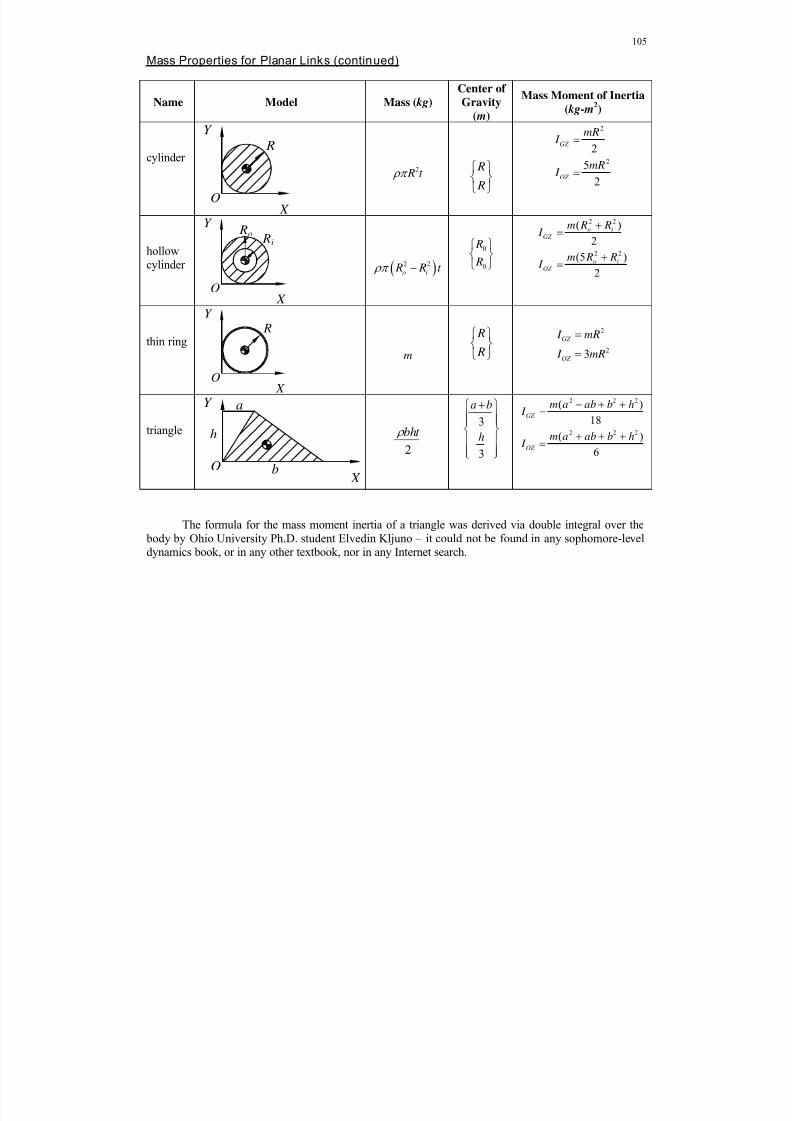
8/11/2019 Mechanism kinematics & dynamics.pdf
http://slidepdf.com/reader/full/mechanism-kinematics-dynamicspdf 105/269
105
Mass Properties for Planar Links (continued)
Name Model Mass ( kg)
Center of
Gravity
( m)
Mass Moment of Inertia
( kg- m2)
cylinder2 R t
R
R
2
22
5
2
GZ
OZ
mR I
mR I
hollowcylinder 2 2
o i R R t
0
0
R
R
2 2
2 2
( )
2
(5 )
2
o iGZ
o iOZ
m R R I
m R R I
thin ringm
R
R
2
23
GZ
OZ
I mR
I mR
triangle
2
bht
3
3
a b
h
2 2 2
2 2 2
( )
18
( )
6
GZ
OZ
m a ab b h I
m a ab b h I
The formula for the mass moment inertia of a triangle was derived via double integral over the body by Ohio University Ph.D. student Elvedin Kljuno – it could not be found in any sophomore-leveldynamics book, or in any other textbook, nor in any Internet search.
X
Y
O
R
X
Y
O
Ri
Ro
X
Y
O
R
X
Y
O
h
a
b
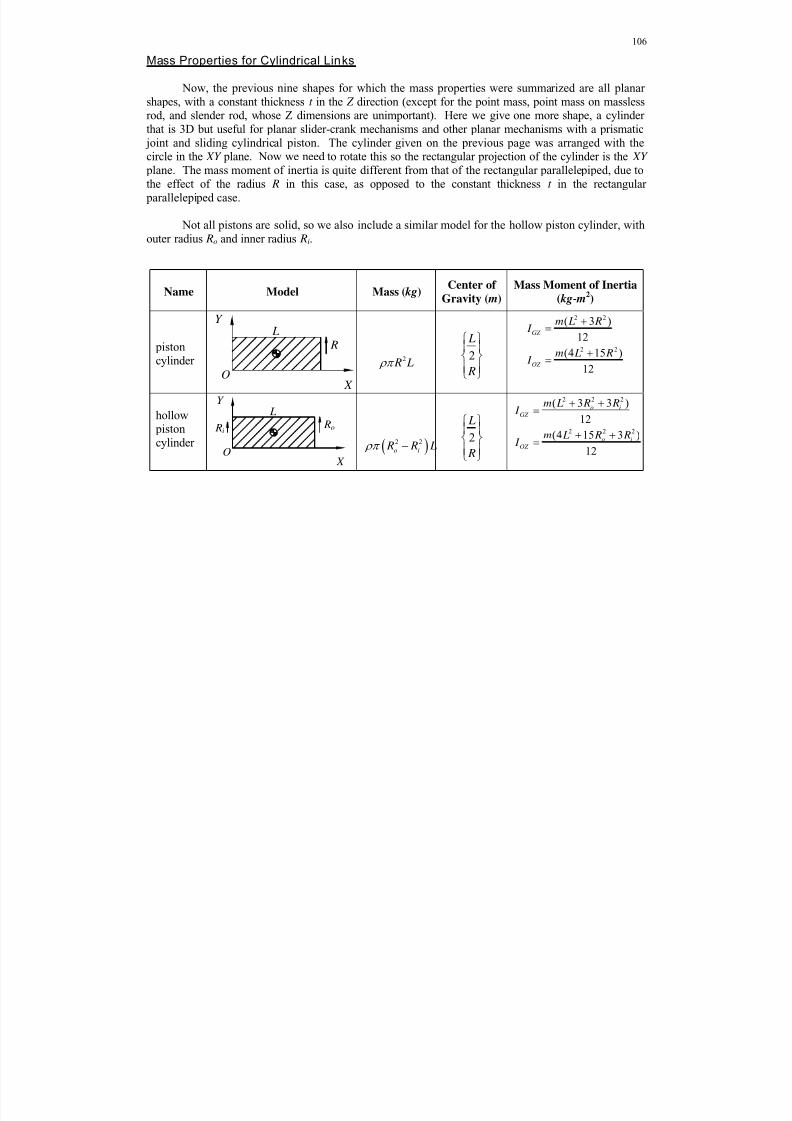
8/11/2019 Mechanism kinematics & dynamics.pdf
http://slidepdf.com/reader/full/mechanism-kinematics-dynamicspdf 106/269
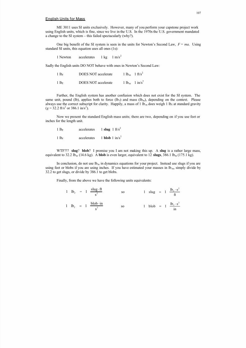
8/11/2019 Mechanism kinematics & dynamics.pdf
http://slidepdf.com/reader/full/mechanism-kinematics-dynamicspdf 107/269
107
English Units for Mass
ME 3011 uses SI units exclusively. However, many of you perform your capstone project workusing English units, which is fine, since we live in the U.S. In the 1970s the U.S. government mandateda change to the SI system – this failed spectacularly (why?).
One big benefit of the SI system is seen in the units for Newton’s Second Law, F = ma. Usingstandard SI units, this equation uses all ones (1s):
1 Newton accelerates 1 kg 1 m/s2
Sadly the English units DO NOT behave with ones in Newton’s Second Law:
1 lbf DOES NOT accelerate 1 lbm 1 ft/s2
1 lbf DOES NOT accelerate 1 lbm 1 in/s2
Further, the English system has another confusion which does not exist for the SI system. Thesame unit, pound (lb), applies both to force (lbf ) and mass (lbm), depending on the context. Pleasealways use the correct subscript for clarity. Happily, a mass of 1 lbm does weigh 1 lbf at standard gravity(g = 32.2 ft/s2 or 386.1 in/s2).
Now we present the standard English mass units; there are two, depending on if you use feet orinches for the length unit.
1 lbf accelerates 1 slug 1 ft/s2
1 lbf accelerates 1 blob 1 in/s2
WTF?!? slug? blob? I promise you I am not making this up. A slug is a rather large mass,equivalent to 32.2 lbm (14.6 kg). A blob is even larger, equivalent to 12 slugs, 386.1 lbm (175.1 kg).
In conclusion, do not use lbm in dynamics equations for your project. Instead use slugs if you areusing feet or blobs if you are using inches. If you have estimated your masses in lbm, simply divide by32.2 to get slugs, or divide by 386.1 to get blobs.
Finally, from the above we have the following units equivalents:
f 2
slug ft1 lb 1s
so2
f lb s1 slug 1
ft
f 2
blob in1 lb 1
s
so
2
f lb s1 blob 1
in

8/11/2019 Mechanism kinematics & dynamics.pdf
http://slidepdf.com/reader/full/mechanism-kinematics-dynamicspdf 108/269
108
3.4 Four-Bar Mechanism Inverse Dynamics Analysis
Here are the link 2 and 4 details for the four-bar inverse dynamics matrix from the NotesBook.
Link 2 details Link 4 details
2 2 212
12
2 2 212
12 2 2
32 12 2
12 2 2
cos( )
sin( )
cos
sin
G X
GY
X
Y
Rr r
Rr
r r r r r
r r
4 4 414
14
4 4 414
14 4 4
34 14 4
14 4 4
cos( )
sin( )
cos
sin
G X
GY
X
Y
Rr r
Rr
r r r r r
r r
22 2 2 2 2 2 2 2 2
2 22 2 2 2 2 2 2 2 2
sin( ) cos( )
cos( ) sin( )
G X G G
G
G Y G G
A R R A
A R R
24 4 4 4 4 4 4 4 4
4 24 4 4 4 4 4 4 4 4
sin( ) cos( )
cos( ) sin( )
G X G G
G
G Y G G
A R R A
A R R
4
4
4 4 4
44 4 4
44
4
4 4
cos
sin
cos
sin
E
E
E X E E
E E Y E E
E r E X
E
E Y E r
F F F
F F
r r r
r r
4 4ˆ
E E M M k
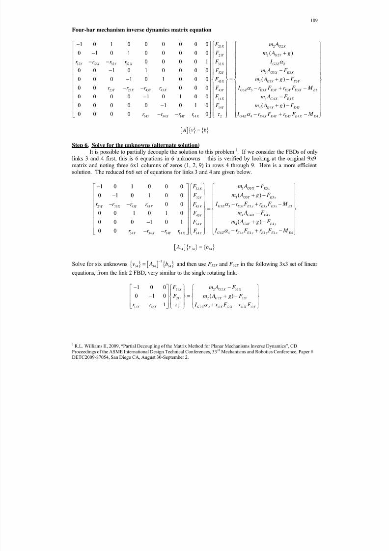
8/11/2019 Mechanism kinematics & dynamics.pdf
http://slidepdf.com/reader/full/mechanism-kinematics-dynamicspdf 109/269
109
Four-bar mechanism inverse dynamics matrix equation
21
21
12 12 32 32 32
32
43
23 23 43 43 43
14
14
34 34 14 14 2
1 0 1 0 0 0 0 0 0
0 1 0 1 0 0 0 0 0
0 0 0 0 1
0 0 1 0 1 0 0 0 0
0 0 0 1 0 1 0 0 0
0 0 0 0 0
0 0 0 0 1 0 1 0 0
0 0 0 0 0 1 0 1 0
0 0 0 0 0
X
Y
Y X Y X X
Y
X
Y X Y X Y
X
Y
Y X Y X
F
F
r r r r F
F
F
r r r r F
F
F
r r r r
2 2
2 2
2 2
3 3 3
3 3 3
3 3 3 3 3 3 3
4 4 4
4 4 4
4 4 4 4 4 4 4
( )
( )
( )
G X
G Y
G Z
G X E X
G Y E Y
G Z E X E Y E Y E X E
G X E X
G Y E Y
G Z E X E Y E Y E X E
m A
m A g
I
m A F
m A g F
I r F r F M
m A F
m A g F
I r F r F M
A v b
Step 6. Solve for the unknowns (alternate solution)
It is possible to partially decouple the solution to this problem1. If we consider the FBDs of onlylinks 3 and 4 first, this is 6 equations in 6 unknowns – this is verified by looking at the original 9x9matrix and noting three 6x1 columns of zeros (1, 2, 9) in rows 4 through 9. Here is a more efficientsolution. The reduced 6x6 set of equations for links 3 and 4 are given below.
3 3 332
3 3 332
3 3 3 3 3 3 323 23 43 43 43
4 4 443
14
34 34 14 14 14
1 0 1 0 0 0
( )0 1 0 1 0 0
0 0
0 0 1 0 1 0
0 0 0 1 0 10 0
G X E x X
G Y E yY
G Z E x E y E y E x E Y X Y X X
G X E xY
X
Y X Y X Y
m A F F
m A g F F
I r F r F M r r r r F
m A F F
F r r r r F
4 4 4
4 4 4 4 4 4 4
( )G Y E y
G Z E x E y E y E x E
m A g F I r F r F M
34 34 34 A v b
Solve for six unknowns 1
34 34 34v A b
and then use F 32 X and F 32Y in the following 3x3 set of linear
equations, from the link 2 FBD, very similar to the single rotating link.
21 2 2 32
21 2 2 32
12 12 2 2 2 32 32 32 32
1 0 0
0 1 0 ( )1
X G X X
Y G Y Y
Y X G Z Y X X Y
F m A F
F m A g F r r I r F r F
1 R.L. Williams II, 2009, “Partial Decoupling of the Matrix Method for Planar Mechanisms Inverse Dynamics”, CDProceedings of the ASME International Design Technical Conferences, 33rd Mechanisms and Robotics Conference, Paper #DETC2009-87054, San Diego CA, August 30-September 2.
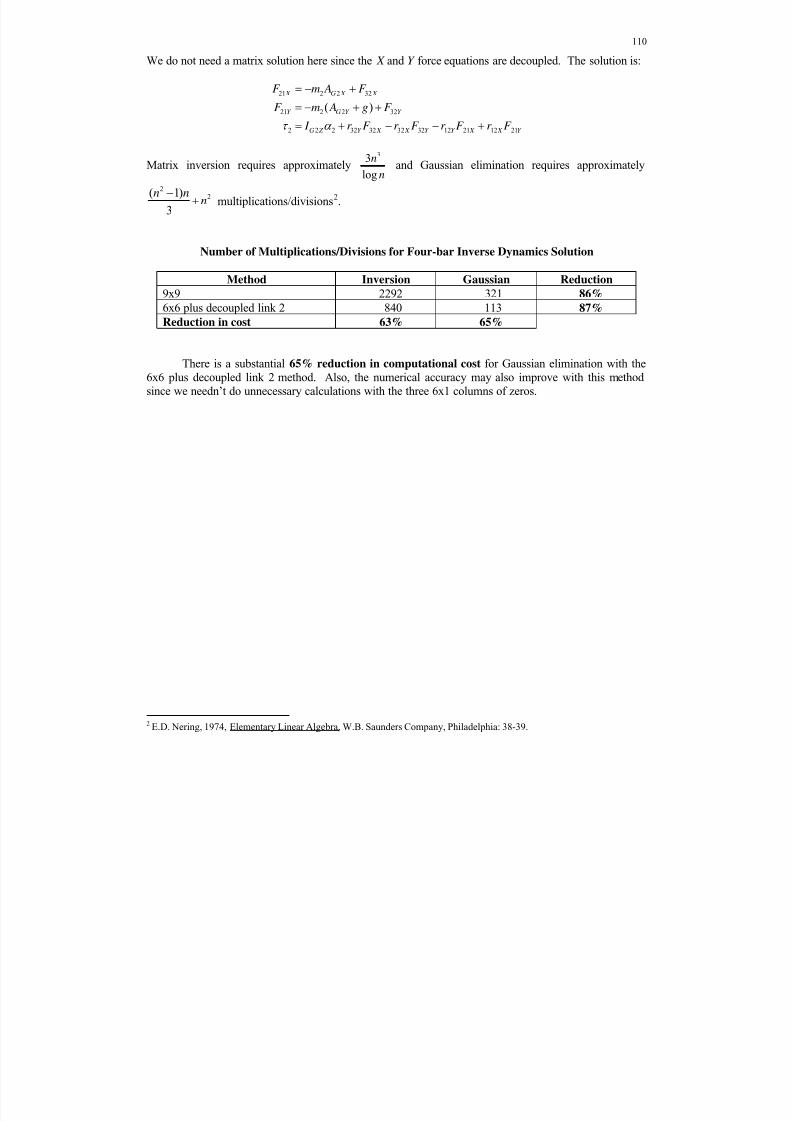
8/11/2019 Mechanism kinematics & dynamics.pdf
http://slidepdf.com/reader/full/mechanism-kinematics-dynamicspdf 110/269
110
We do not need a matrix solution here since the X and Y force equations are decoupled. The solution is:
21 2 2 32
21 2 2 32
2 2 2 32 32 32 32 12 21 12 21
( )
X G X X
Y G Y Y
G Z Y X X Y Y X X Y
F m A F
F m A g F
I r F r F r F r F
Matrix inversion requires approximately33
log
n
n and Gaussian elimination requires approximately
22( 1)
3
n nn
multiplications/divisions2.
Number of Multiplications/Divisions for Four-bar Inverse Dynamics Solution
Method Inversion Gaussian Reduction
9x9 2292 321 86%
6x6 plus decoupled link 2 840 113 87%
Reduction in cost 63% 65%
There is a substantial 65% reduction in computational cost for Gaussian elimination with the6x6 plus decoupled link 2 method. Also, the numerical accuracy may also improve with this methodsince we needn’t do unnecessary calculations with the three 6x1 columns of zeros.
2 E.D. Nering, 1974, Elementary Linear Algebra, W.B. Saunders Company, Philadelphia: 38-39.
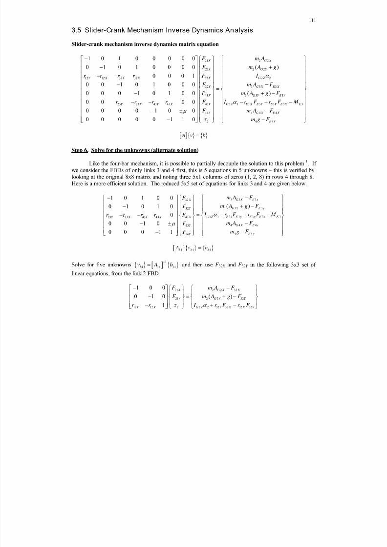
8/11/2019 Mechanism kinematics & dynamics.pdf
http://slidepdf.com/reader/full/mechanism-kinematics-dynamicspdf 111/269
111
3.5 Slider-Crank Mechanism Inverse Dynamics Analysis
Slider-crank mechanism inverse dynamics matrix equation
21 2 2
21 2 2
3212 12 32 32
32
43
4323 23 43 43
14
2
1 0 1 0 0 0 0 0
( )0 1 0 1 0 0 0 0
0 0 0 1
0 0 1 0 1 0 0 0
0 0 0 1 0 1 0 0
0 0 0 0
0 0 0 0 1 0 0
0 0 0 0 0 1 1 0
X G X
Y G Y
X GY X Y X
Y
X
Y Y X Y X
Y
F m A
F m A g
F I r r r r
F
F
F r r r r
F
2 2
3 3 3
3 3 3
3 3 3 3 3 3 3
4 4 4
4 4
( )
Z
G X E X
G Y E Y
G Z E X E Y E Y E X E
G X E X
E Y
m A F
m A g F
I r F r F M
m A F
m g F
A v b
Step 6. Solve for the unknowns (alternate solution)
Like the four-bar mechanism, it is possible to partially decouple the solution to this problem1. Ifwe consider the FBDs of only links 3 and 4 first, this is 5 equations in 5 unknowns – this is verified bylooking at the original 8x8 matrix and noting three 5x1 columns of zeros (1, 2, 8) in rows 4 through 8.Here is a more efficient solution. The reduced 5x5 set of equations for links 3 and 4 are given below.
3 3 332
3 3 332
3 3 3 3 3 3 34323 23 43 43
4 4 443
4 414
1 0 1 0 0
( )0 1 0 1 0
0
0 0 1 0
0 0 0 1 1
G X E x X
G Y E yY
G Z E x E y E y E x E X Y X Y X
G X E xY
E yY
m A F F
m A g F F
I r F r F M F r r r r
m A F F
m g F F
34 34 34 A v b
Solve for five unknowns 1
34 34 34v A b
and then use F 32 X and F 32Y in the following 3x3 set of
linear equations, from the link 2 FBD.
21 2 2 32
21 2 2 32
12 12 2 2 2 32 32 32 32
1 0 0
0 1 0 ( )
1
X G X X
Y G Y Y
Y X G Z Y X X Y
F m A F
F m A g F
r r I r F r F

8/11/2019 Mechanism kinematics & dynamics.pdf
http://slidepdf.com/reader/full/mechanism-kinematics-dynamicspdf 112/269
112
We do not need a matrix solution here since the X and Y force equations are decoupled. The solution isidentical to that of the four-bar mechanism.
21 2 2 32
21 2 2 32
2 2 2 32 32 32 32 12 21 12 21
( )
X G X X
Y G Y Y
G Z Y X X Y Y X X Y
F m A F
F m A g F
I r F r F r F r F
Matrix inversion requires approximately33
log
n
n and Gaussian elimination requires approximately
22( 1)
3
n nn
multiplications/divisions (Nering, 1974).
Number of Multiplications/Divisions for Slider-Crank Inverse Dynamics Solution
Method Inversion Gaussian Reduction
8x8 1701 232 86%
5x5 plus decoupled link 2 544 72 87%
Reduction in cost 68% 69%
There is a substantial 69% reduction in computational cost for Gaussian elimination with the5x5 plus decoupled link 2 method. Also, the numerical accuracy may also improve with this methodsince we needn’t do unnecessary calculations with the three 5x1 columns of zeros.

8/11/2019 Mechanism kinematics & dynamics.pdf
http://slidepdf.com/reader/full/mechanism-kinematics-dynamicspdf 113/269
113
3.6 Inverted Slider-Crank Mechanism Inverse Dynamics Analysis
This problem can be solved with a 9x9 matrix, after eliminating a redundant equation. Let’s trya simpler approach – assume the link 3 mass is small and use only FBDs for links 2 and 4. We furtherassume zero external forces and moments.
Step 1. The inverted slider-crank Position, Velocity, and Acceleration Analyses must be complete.
Step 2. Draw the Inverted Slider-Crank Mechanism Free-Body Diagrams
ijF unknown vector internal joint force of link i acting on link j.
ijr known vector moment arm pointing to the joint connection with link i from the CG of link j.

8/11/2019 Mechanism kinematics & dynamics.pdf
http://slidepdf.com/reader/full/mechanism-kinematics-dynamicspdf 114/269
114
Step 3. State the Problem
Given r 1, 1 = 0 , r 2
2, r 4, 4
2, 4r , 4
2, 4r , 4
assume zero external forces and moments
Find 21F , 42F , 14F and 2
Step 4. Derive the Newton-Euler Dynamics Equations.
Newton's Second Law
Link 2
2 42 21 22 2 GF F F W m A
Link 4
4 14 42 44 4 GF F F W m A
Euler's Rotational Dynamics Equation
Link 2
2 42 42 12 212 22G z G Z M r F r F I
Link 4
4 14 14 24 42 44G z G Z M r F r F I
Count the number of unknowns and the number of equations: 6 scalar equations and 7 scalar unknowns.
We need an additional equation; let us assume zero friction between links 2 and 4. Therefore, 42F is
always perpendicular to link 4 and there is only one unknown from this vector, the magnitude F 42.
42 42 4
42
42 42 4
cos( 2)sin( 2)
X
Y
F F F F F

8/11/2019 Mechanism kinematics & dynamics.pdf
http://slidepdf.com/reader/full/mechanism-kinematics-dynamicspdf 115/269
115
Step 5. Derive the XYZ scalar dynamics equations from the vector dynamics equations.
Link 2
42 21 2 2
42 21 2 2
2 42 42 42 42 12 21 12 21 2 2
( )
( ) ( )
X X G X
Y Y G Y
X Y Y X X Y Y X G Z
F F m A
F F m A g
r F r F r F r F I
Link 4
14 42 4 4
14 42 4 4
14 14 14 14 24 42 24 42 4 4
X X G X
Y Y G Y
X Y Y X X Y Y X G Z
F F m A
F F m A g
r F r F r F r F I
Express these scalar equations in matrix/vector form. The simplified inverted slider-crank mechanisminverse dynamics matrix equation is given below.
2 221
2 221
2 212 12 42 42 42
4 414
4 414
4 424 24 14 14 2
1 0 0 0 0
( )0 1 0 0 0
0 0 1
0 0 1 0 0
( )0 0 0 1 0
0 0 0
G X X
G Y Y
G Z Y X X Y
G X X
G Y Y
G Z X Y Y X
m Ac F
m A gs F
I r r r s r c F
m Ac F
m A gs F
I r s r c r r
where:4
4
cos( 2)
sin( 2)
c
s
A v b
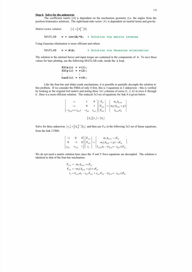
8/11/2019 Mechanism kinematics & dynamics.pdf
http://slidepdf.com/reader/full/mechanism-kinematics-dynamicspdf 116/269
116
Step 6. Solve for the unknowns The coefficient matrix [ A] is dependent on the mechanism geometry (i.e. the angles from the
position kinematics solution). The right-hand-side vector {b} is dependent on inertial terms and gravity.
Matrix/vector solution 1
v A b
MATLAB v = inv(A)*b; % Solution via matrix inverse
Using Gaussian elimination is more efficient and robust.
MATLAB v = A\b; % Solution via Gaussian elimination
The solution to the internal forces and input torque are contained in the components of v. To save these
values for later plotting, use the following MATLAB code, inside the i loop.
f21x(i) = v(1);f21y(i) = v(2);
tau2(i) = v(6);
Like the four-bar and slider-crank mechanisms, it is possible to partially decouple the solution tothis problem. If we consider the FBDs of only 4 first, this is 3 equations in 3 unknowns – this is verified by looking at the original 6x6 matrix and noting three 3x1 columns of zeros (1, 2, 6) in rows 4 through6. Here is a more efficient solution. The reduced 3x3 set of equations for link 4 is given below.
42 4 4
14 4 4
24 24 14 14 14 4 4
1 0
0 1 ( )
G X
X G Y
X Y Y X Y G Z
c F m A
s F m A g
r s r c r r F I
4 4 4 A v b
Solve for three unknowns 1
4 4 4v A b
and then use F 42 in the following 3x3 set of linear equations,
from the link 2 FBD.
21 2 2 42
21 2 2 42
12 12 2 2 2 42 42 42
1 0 0
0 1 0 ( )
1 ( )
X G X
Y G Y
Y X G Z X Y
F m A cF
F m A g sF
r r I r s r c F
We do not need a matrix solution here since the X and Y force equations are decoupled. The solution isidentical to that of the four-bar mechanism.
21 2 2 42
21 2 2 42
2 2 2 12 21 12 21 42 42 42
( )
( )
X G X
Y G Y
G Z Y X X Y X Y
F m A cF
F m A g sF
I r F r F r s r c F

8/11/2019 Mechanism kinematics & dynamics.pdf
http://slidepdf.com/reader/full/mechanism-kinematics-dynamicspdf 117/269
117
Matrix inversion requires approximately33
log
n
n and Gaussian elimination requires approximately
22( 1)
3
n nn
multiplications/divisions (Nering, 1974).
Number of Multiplications/Divisions
Method Inversion Gaussian Reduction
6x6 833 106 87%
3x3 plus decoupled link 2 177 24 86%
Reduction in cost 79% 77%
There is a substantial 77% reduction in computational cost for Gaussian elimination with the 3x3 plusdecoupled link 2 method. Also, the numerical accuracy may also improve with this method since weneedn’t do unnecessary calculations with the three 3x1 columns of zeros.
Step 7. Calculate Shaking Force and Moment
After the basic inverse dynamics problem is solved, we can calculate the vector shaking forceand vector shaking moment, which is the force/moment reaction on the ground link due to the motion,inertia, weight, and external loads (which we assumed to be zero in this problem). The shaking forceand moment for the inverted slider-crank mechanism is identical to the four-bar in notation and terms.
Ground link force/moment diagram
Shaking force
21 14
21 41 21 14
21 14
X X
S
Y Y
F F F F F F F
F F
Shaking moment
2 21 21 41 14
2 21 21 21 21 41 14 41 14
S
X Y Y X X Y Y X
M r F r F
r F r F r F r F
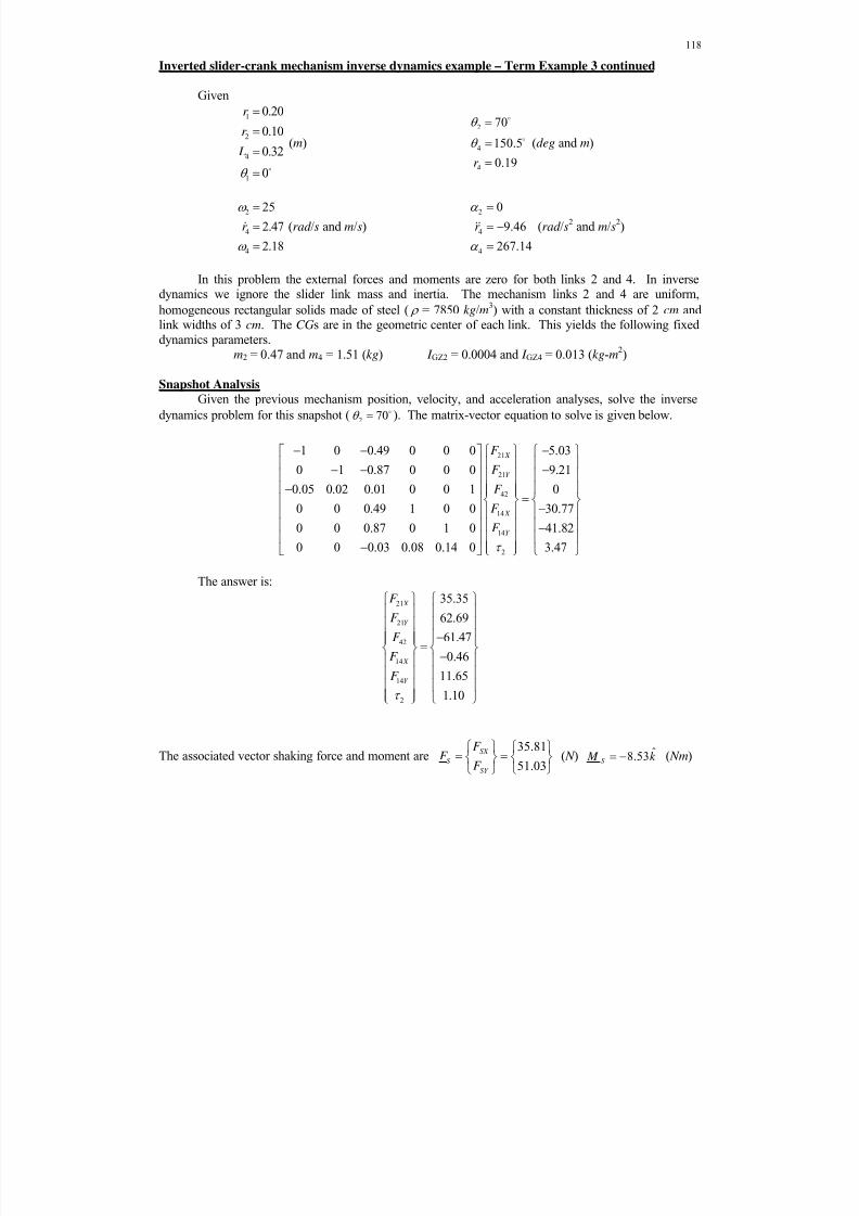
8/11/2019 Mechanism kinematics & dynamics.pdf
http://slidepdf.com/reader/full/mechanism-kinematics-dynamicspdf 118/269
118
Inverted slider-crank mechanism inverse dynamics example – Term Example 3 continued
Given
1
2
4
1
0.20
0.10
0.32
0
r
r
L
(m)
2
4
4
70
150.5
0.19r
(deg and m)
2
4
4
25
2.47
2.18
r
(rad /s and m/s)
2
4
4
0
9.46
267.14
r
(rad /s2 and m/s2)
In this problem the external forces and moments are zero for both links 2 and 4. In inversedynamics we ignore the slider link mass and inertia. The mechanism links 2 and 4 are uniform,
homogeneous rectangular solids made of steel ( = 7850 kg/m3) with a constant thickness of 2 cm and
link widths of 3 cm. The CGs are in the geometric center of each link. This yields the following fixeddynamics parameters.m2 = 0.47 and m4 = 1.51 (kg) I GZ2 = 0.0004 and I GZ4 = 0.013 (kg-m
2)
Snapshot Analysis
Given the previous mechanism position, velocity, and acceleration analyses, solve the inverse
dynamics problem for this snapshot (2 70 ). The matrix-vector equation to solve is given below.
21
21
42
14
14
2
1 0 0.49 0 0 0 5.03
0 1 0.87 0 0 0 9.21
0.05 0.02 0.01 0 0 1 00 0 0.49 1 0 0 30.77
0 0 0.87 0 1 0 41.82
0 0 0.03 0.08 0.14 0 3.47
X
Y
X
Y
F
F
F F
F
The answer is:
21
21
42
14
14
2
35.35
62.69
61.47
0.4611.65
1.10
X
Y
X
Y
F
F
F
F F
The associated vector shaking force and moment are35.81
51.03
SX
S
SY
F F
F
( N ) ˆ8.53S M k ( Nm)
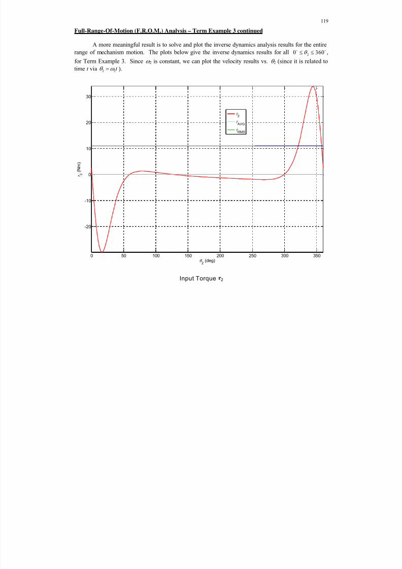
8/11/2019 Mechanism kinematics & dynamics.pdf
http://slidepdf.com/reader/full/mechanism-kinematics-dynamicspdf 119/269
119
Full-Range-Of-Motion (F.R.O.M.) Analysis – Term Example 3 continued
A more meaningful result is to solve and plot the inverse dynamics analysis results for the entire
range of mechanism motion. The plots below give the inverse dynamics results for all20 360 ,
for Term Example 3. Since 2 is constant, we can plot the velocity results vs. 2 (since it is related to
time t via 2 2t ).
Input Torque 2
0 50 100 150 200 250 300 350
-20
-10
0
10
20
30
2 (deg)
2
( N m )
2
AVG
RMS
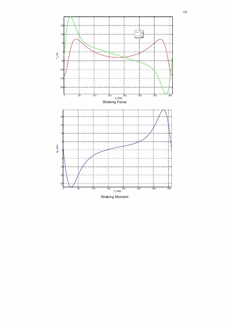
8/11/2019 Mechanism kinematics & dynamics.pdf
http://slidepdf.com/reader/full/mechanism-kinematics-dynamicspdf 120/269
120
Shaking Force
Shaking Moment
0 50 100 150 200 250 300 350
-200
-150
-100
-50
0
50
100
150
2 (deg)
F S
( N )
FSX
FSY
0 50 100 150 200 250 300 350
-20
-15
-10
-5
0
5
10
15
20
2 (deg)
M S
( N m )

8/11/2019 Mechanism kinematics & dynamics.pdf
http://slidepdf.com/reader/full/mechanism-kinematics-dynamicspdf 121/269
121
3.7 Multi-loop Mechanism Inverse Dynamics Analysis
The Matrix Method can be applied to any planar mechanism inverse dynamics problem. Hereare the five two-loop six-bar mechanisms from Dr. Bob’s on-line Mechanism Atlas.
Stephenson I 6-Bar Mechanism
Stephenson II 6-Bar Mechanism Stephenson III 6-Bar Mechanism
Watt I 6-Bar Mechanism Watt II 6-Bar Mechanism
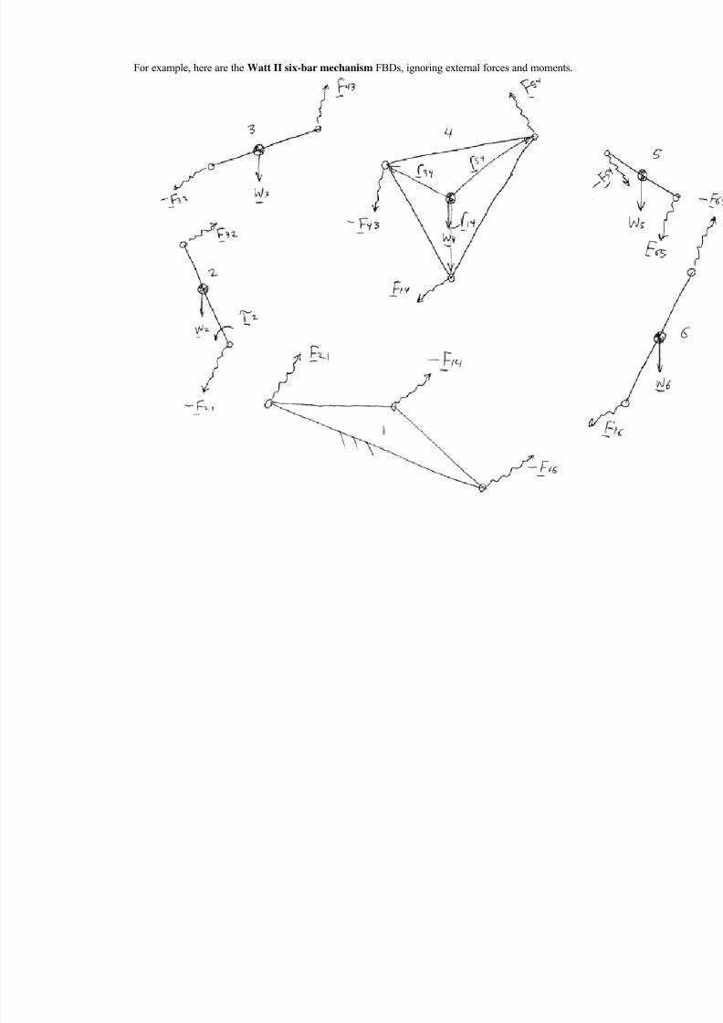
8/11/2019 Mechanism kinematics & dynamics.pdf
http://slidepdf.com/reader/full/mechanism-kinematics-dynamicspdf 122/269
For example, here are the Watt II six-bar mechanism FBDs, ignoring external forces and moments.
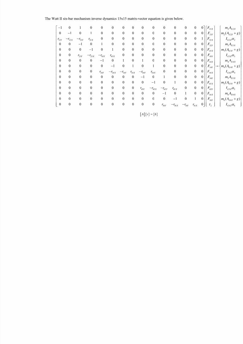
8/11/2019 Mechanism kinematics & dynamics.pdf
http://slidepdf.com/reader/full/mechanism-kinematics-dynamicspdf 123/269

8/11/2019 Mechanism kinematics & dynamics.pdf
http://slidepdf.com/reader/full/mechanism-kinematics-dynamicspdf 124/269
124
Step 6. Solve for the unknowns (continued)
Like the four-bar mechanism, it is possible to partially decouple the solution to this problem. Ifwe consider the FBDs of only links 5 and 6 first, this is 6 equations in 6 unknowns – this is verified bylooking at the original 15x15 matrix and noting nine 6x1 columns of zeros (1, 2, 3, 4, 5, 6, 7, 8, 15) inthe six rows 10 through 15. Here is a more efficient solution. The reduced 6x6 set of equations for links5 and 6 is given below.
54 5 5
54 5 5
45 45 65 65 65 5 5
65 6 6
16 6 6
56 56 16 16 16 6 6
1 0 1 0 0 0
0 1 0 1 0 0 ( )
0 0
0 0 1 0 1 0
0 0 0 1 0 1 ( )
0 0
X G X
Y G Y
Y X Y X X G Z
Y G X
X G Y
Y X Y X Y G Z
F m A
F m A g
r r r r F I
F m A
F m A g
r r r r F I
56 56 56 A v b
Solve for the six unknowns 1
56 56 56v A b
. Second, consider the FBDs of only links 3 and 4: thisis 6 equations in 6 unknowns – this is verified by looking at the original 15x15 matrix and noting seven6x1 columns of zeros (1, 2, 11, 12, 13, 14, 15) in the six rows 4 through 9. Recognizing that now F 54 X and F 54Y are now known from the above 6x6 partial solution, here is a more efficient solution. Thereduced 6x6 set of equations for links 3 and 4 is given below.
3 332
3 332
23 23 43 43 3 343
4 4 5443
4 4 5414
34 34 14 14 4 4 54 5414
1 0 1 0 0 0
0 1 0 1 0 0 ( )
0 0
0 0 1 0 1 0
0 0 0 1 0 1 ( )0 0
G X X
G Y Y
Y X Y X G Z X
G X X Y
G Y Y X
Y X Y X G Z Y X Y
m AF
m A gF
r r r r I F
m A F F
m A g F F r r r r I r F r F
54 54 X Y F
34 34 34 A v b
Solve for six unknowns 1
34 34 34v A b
and then use F 32 X and F 32Y in the following 3x3 set of linear
equations, from the link 2 FBD.
21 2 2 32
21 2 2 32
12 12 2 2 2 32 32 32 32
1 0 0
0 1 0 ( )
1
X G X X
Y G Y Y
Y X G Z Y X X Y
F m A F
F m A g F
r r I r F r F
We do not need a matrix solution here since the X and Y force equations are decoupled. The solution isidentical to that of the four-bar mechanism.
21 2 2 32
21 2 2 32
2 2 2 32 32 32 32 12 21 12 21
( )
X G X X
Y G Y Y
G Z Y X X Y Y X X Y
F m A F
F m A g F
I r F r F r F r F
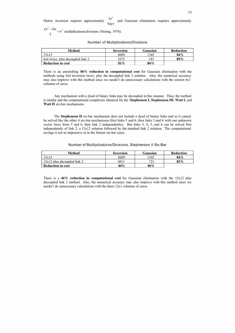
8/11/2019 Mechanism kinematics & dynamics.pdf
http://slidepdf.com/reader/full/mechanism-kinematics-dynamicspdf 125/269
125
Matrix inversion requires approximately33
log
n
n and Gaussian elimination requires approximately
22( 1)
3
n nn
multiplications/divisions (Nering, 1974).
Number of Multiplications/Divisions
Method Inversion Gaussian Reduction
15x15 8609 1345 84%
6x6 twice, plus decoupled link 2 1672 183 89%
Reduction in cost 81% 86%
There is an astonishing 86% reduction in computational cost for Gaussian elimination with themethods using 6x6 inversion twice, plus the decoupled link 2 solution. Also, the numerical accuracymay also improve with this method since we needn’t do unnecessary calculations with the sixteen 6x1columns of zeros.
Any mechanism with a dyad of binary links may be decoupled in this manner. Thus, the methodis similar and the computational complexity identical for the Stephenson I, Stephenson III, Watt I, andWatt II six-bar mechanisms.
The Stephenson II six-bar mechanism does not include a dyad of binary links and so it cannot be solved like the other 4 six-bar mechanisms (first links 5 and 6, then links 3 and 4 with one unknownvector force from 5 and 6, then link 2 independently). But links 3, 4, 5, and 6 can be solved firstindependently of link 2: a 12x12 solution followed by the standard link 2 solution. The computationalsavings is not as impressive as in the former six-bar cases.
Number of Multiplications/Divisions, Stephenson II Six-Bar
Method Inversion Gaussian Reduction
15x15 8609 1345 84%
12x12 plus decoupled link 2 4811 723 85%
Reduction in cost 44% 46%
There is a 46% reduction in computational cost for Gaussian elimination with the 12x12 plusdecoupled link 2 method. Also, the numerical accuracy may also improve with this method since weneedn’t do unnecessary calculations with the three 12x1 columns of zeros.
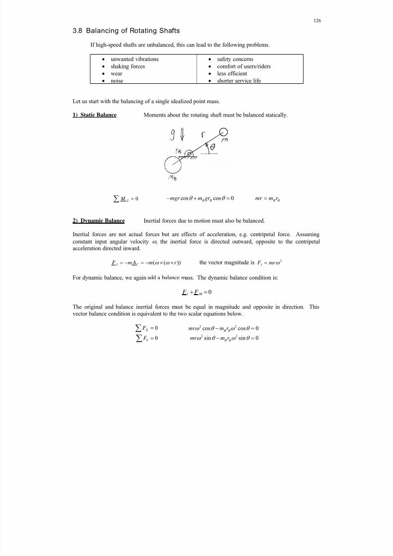
8/11/2019 Mechanism kinematics & dynamics.pdf
http://slidepdf.com/reader/full/mechanism-kinematics-dynamicspdf 126/269
126
3.8 Balancing of Rotating Shafts
If high-speed shafts are unbalanced, this can lead to the following problems.
unwanted vibrations
shaking forces
wear noise
safety concerns
comfort of users/riders
less efficient shorter service life
Let us start with the balancing of a single idealized point mass.
1) Static Balance Moments about the rotating shaft must be balanced statically.
0 Z M cos cos 0 B Bmgr m gr B Bmr m r
2) Dynamic Balance Inertial forces due to motion must also be balanced.
Inertial forces are not actual forces but are effects of acceleration, e.g. centripetal force. Assuming
constant input angular velocity , the inertial force is directed outward, opposite to the centripetalacceleration directed inward.
( ( )) I C F m A m r the vector magnitude is 2
I F mr
For dynamic balance, we again add a balance mass. The dynamic balance condition is:
0 I IBF F
The original and balance inertial forces must be equal in magnitude and opposite in direction. Thisvector balance condition is equivalent to the two scalar equations below.
0
0
X
Y
F
F
2 2
2 2
cos cos 0
sin sin 0
B B
B B
mr m r
mr m r
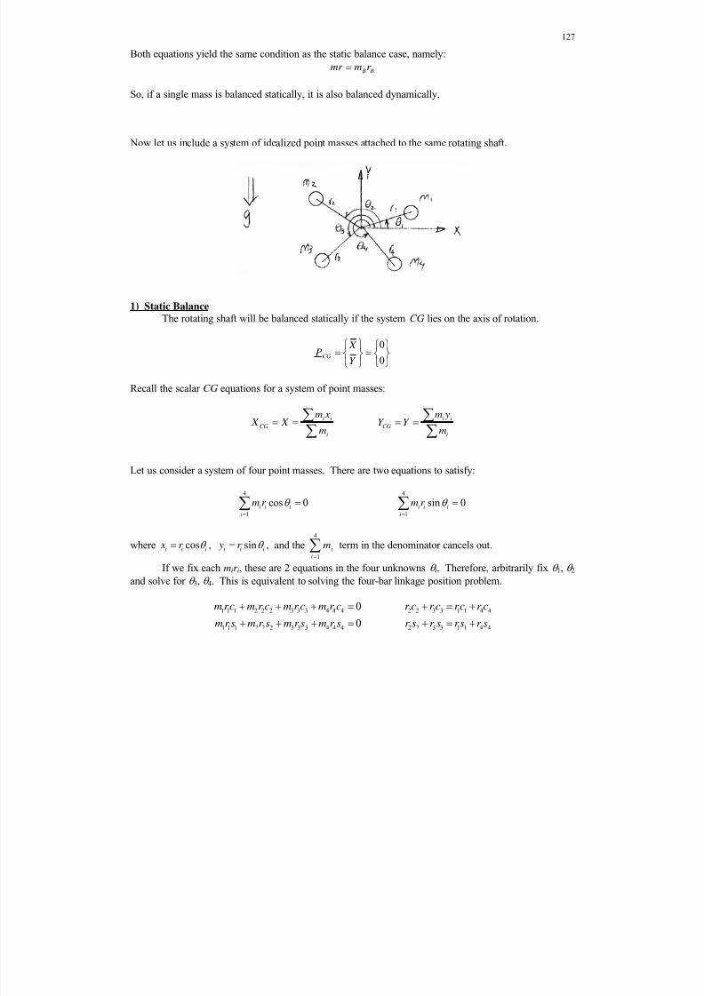
8/11/2019 Mechanism kinematics & dynamics.pdf
http://slidepdf.com/reader/full/mechanism-kinematics-dynamicspdf 127/269
127
Both equations yield the same condition as the static balance case, namely:
B Bmr m r
So, if a single mass is balanced statically, it is also balanced dynamically.
Now let us include a system of idealized point masses attached to the same rotating shaft.
1) Static Balance The rotating shaft will be balanced statically if the system CG lies on the axis of rotation.
0
0CG
X P
Y
Recall the scalar CG equations for a system of point masses:
i i
CG
i
m x X X
m
i i
CG
i
m yY Y
m
Let us consider a system of four point masses. There are two equations to satisfy:
4
1
cos 0i i i
i
m r
4
1
sin 0i i i
i
m r
where cosi i i x r , sini i i
y r , and the4
1
i
i
m
term in the denominator cancels out.
If we fix each mir i, these are 2 equations in the four unknowns i. Therefore, arbitrarily fix 1, 2
and solve for 3, 4. This is equivalent to solving the four-bar linkage position problem.
1 1 1 2 2 2 3 3 3 4 4 4
1 1 1 2 2 2 3 3 3 4 4 4
0
0
m rc m r c m r c m r c
m r s m r s m r s m r s
2 2 3 3 1 1 4 4
2 2 3 3 1 1 4 4
r c r c rc r c
r s r s r s r s
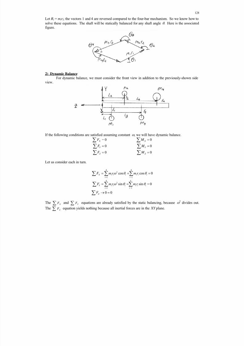
8/11/2019 Mechanism kinematics & dynamics.pdf
http://slidepdf.com/reader/full/mechanism-kinematics-dynamicspdf 128/269
128
Let Ri = mir i; the vectors 1 and 4 are reversed compared to the four-bar mechanism. So we know how to
solve these equations. The shaft will be statically balanced for any shaft angle . Here is the associatedfigure.
2) Dynamic Balance For dynamic balance, we must consider the front view in addition to the previously-shown side
view.
If the following conditions are satisfied assuming constant , we will have dynamic balance.
00
0
X
Y
Z
F
F
F
00
0
X
Y
Z
M
M
M
Let us consider each in turn.
4 42
1 1
4 42
1 1
cos cos 0
sin sin 0
0 0
X i i i i i i
i i
Y i i i i i i
i i
Z
F m r m r
F m r m r
F
The X
F andY
F equations are already satisfied by the static balancing, because 2 divides out.
The Z
F equation yields nothing because all inertial forces are in the XY plane.
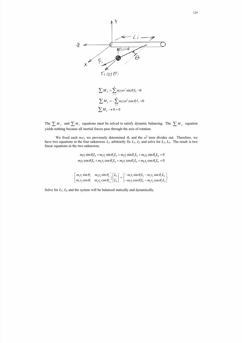
8/11/2019 Mechanism kinematics & dynamics.pdf
http://slidepdf.com/reader/full/mechanism-kinematics-dynamicspdf 129/269
129
42
1
42
1
sin 0
cos 0
0 0
X i i i ii
Y i i i i
i
Z
M m r L
M m r L
M
The X
M andY
M equations must be solved to satisfy dynamic balancing. The Z
M equation
yields nothing because all inertial forces pass through the axis of rotation.
We fixed each mir i, we previously determined i, and the
2
term divides out. Therefore, wehave two equations in the four unknowns Li; arbitrarily fix L1, L2 and solve for L3, L4. The result is twolinear equations in the two unknowns.
1 1 1 1 2 2 2 2 3 3 3 3 4 4 4 4
1 1 1 1 2 2 2 2 3 3 3 3 4 4 4 4
sin sin sin sin 0
cos cos cos cos 0
m r L m r L m r L m r L
m r L m r L m r L m r L
3 3 3 4 4 4 3 1 1 1 1 2 2 2 2
3 3 3 4 4 4 4 1 1 1 1 2 2 2 2
sin sin sin sin
cos cos cos cos
m r m r L m r L m r L
m r m r L m r L m r L
Solve for L3, L4 and the system will be balanced statically and dynamically.

8/11/2019 Mechanism kinematics & dynamics.pdf
http://slidepdf.com/reader/full/mechanism-kinematics-dynamicspdf 130/269
130
3.9 Inverse Dynamics Analysis Examples
This section presents complete snapshot and full-range-of-motion (F.R.O.M.) examples todemonstrate the inverse dynamics analyses in the ME 3011 NotesBook. The first example is for thesingle rotating link inverse dynamics (whose kinematics were not yet presented). Term Example 1 isfor the four-bar mechanism and Term Example 2 is for the slider-crank mechanism. The latter twoexamples are continuations for the Term Example 1 and 2 kinematics examples presented earlier in thisME 3011 NotesBook Supplement.
3.9.1 Single Rotating Link Inverse Dynamics Example
Given: L = 1, h = 0.1 m, m = 2 kg, = 100 rad/s, = 0, F E = 150 N, E = 0, M E = 0 Nm.
Calculated terms 12 0.5 E r r m I GZ = 0.17 kgm
2
Snapshot inverse dynamics analysis
At 150 , given this link, motion, and external force, calculate 12 12, , X Y F F and ,S S F M .
4330
2500
Gx
Gy
A
A
2
m
s
12
12
1 0 0 8510
0 1 0 4980
0.250 0.433 1 37.5
X
Y
F
F
12
12
8510
4980
66.5
X
Y
F
F
N, Nm
21 12
8510
4980S F F F
N ˆ66.5S M k Nm
Full-Range-Of-Motion (F.R.O.M.) Analysis
A more meaningful result from inverse dynamics analysis is to solve and plot the dynamicsunknowns for the entire range of mechanism motion. For the same example as the snapshot we specify
that the given is constant. Prior to solving the inverse dynamics problem, the CG translational
acceleration results for all 0 360 are given in the plot below. The X components are red and theY green. Is the static link weight (mg) significant in this problem?
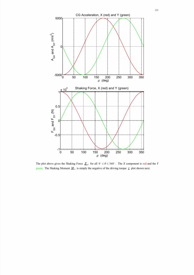
8/11/2019 Mechanism kinematics & dynamics.pdf
http://slidepdf.com/reader/full/mechanism-kinematics-dynamicspdf 131/269
131
The plot above gives the Shaking Force S F for all 0 360 . The X component is red and the Y
green. The Shaking Moment S M is simply the negative of the driving torque plot shown next.
0 50 100 150 200 250 300 350-5000
0
5000
(deg)
A G X
a n d
A G Y
( m / s
2 )
CG Acceleration, X (red) and Y (green)
0 50 100 150 200 250 300 350-1
-0.5
0
0.5
1x 10
4
(deg)
F S X
a n d
F S Y
( N
)
Shaking Force, X (red) and Y (green)
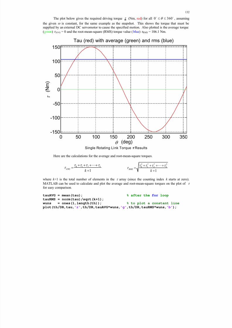
8/11/2019 Mechanism kinematics & dynamics.pdf
http://slidepdf.com/reader/full/mechanism-kinematics-dynamicspdf 132/269
132
The plot below gives the required driving torque (Nm, red ) for all 0 360 , assuming
the given is constant, for the same example as the snapshot. This shows the torque that must besupplied by an external DC servomotor to cause the specified motion. Also plotted is the average torque
(green) AVG = 0 and the root-mean-square (RMS) torque value ( blue) RMS = 106.1 Nm.
Single Rotating Link Torque Results
Here are the calculations for the average and root-mean-square torques.
0 1 2
1
k AVG
k
2 2 2 2
0 1 2
1
k
RMS k
where k +1 is the total number of elements in the array (since the counting index k starts at zero).
MATLAB can be used to calculate and plot the average and root-mean-square torques on the plot of for easy comparison.
tauAVG = mean(tau); % after the for loop tauRMS = norm(tau)/sqrt(k+1);wuns = ones(1,length(th)); % to plot a constant line plot(th/DR,tau,'r',th/DR,tauAVG*wuns,'g',th/DR,tauRMS*wuns,'b');
0 50 100 150 200 250 300 350-150
-100
-50
0
50
100
150
(deg)
( N
m )
Tau (red) with average (green) and rms (blue)
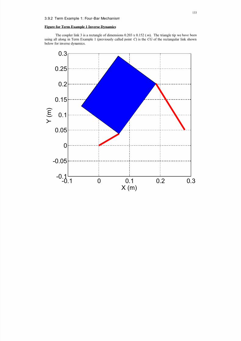
8/11/2019 Mechanism kinematics & dynamics.pdf
http://slidepdf.com/reader/full/mechanism-kinematics-dynamicspdf 133/269
133
3.9.2 Term Example 1: Four-Bar Mechanism
Figure for Term Example 1 Inverse Dynamics
The coupler link 3 is a rectangle of dimensions 0.203 x 0.152 (m). The triangle tip we have beenusing all along in Term Example 1 (previously called point C ) is the CG of the rectangular link shown below for inverse dynamics.
-0.1 0 0.1 0.2 0.3-0.1
-0.05
0
0.05
0.1
0.15
0.2
0.25
0.3
X (m)
Y ( m )

8/11/2019 Mechanism kinematics & dynamics.pdf
http://slidepdf.com/reader/full/mechanism-kinematics-dynamicspdf 134/269
134
Four-bar mechanism inverse dynamics example – Term Example 1 continued This is the mechanism from Term Example 1 (open branch), with kinematics solutions as
presented before. Given r 1 = 0.284, r 2 = 0.076, r 3 = 0.203, r 4 = 0.178, 1 10.3 , 2 30 , 3 53.8 ,
4 121.7 , RG2 = 0.038, RG3 = 0.127, RG4 = 0.089 (m), 2 0 , 3 36.9 , 4 0 , 2 20 , 3 8.09 ,
4 3.73 (rad /s), 2 0 , 3 8.65 , and 4 244.4 (rad /s2).
All moving links are wood, with mass density 830.4 kg/m3. Links 2 and 4 have rectangular
dimensions r i x 0.019 x 0.013 thick (m; i=2,4); link 3 has rectangular dimensions 0.203 x 0.152 x 0.013
thick (m), as shown on the previous page. The calculated mass and inertia parameters are 2 0.015m ,
3 0.327m , 4 0.036m (kg) and 6
2 7.9 10G Z I , 3
3 1.8 10G Z I , 5
4 9.5 10G Z I (kgm
2). All
external forces and moments are zero but gravity, g = 9.81 m/s2, is included.
Snapshot Analysis (one input angle)
At 230 , given this mechanism and motion, calculate the four vector internal joint forces, the
driving torque 2 , and the shaking force and moment ,S S F M for this snapshot.
21
21
32
32
43
43
14
14
1 0 1 0 0 0 0 0 00 1 0 1 0 0 0 0 0
0.019 0.033 0.019 0.033 0 0 0 0 1
0 0 1 0 1 0 0 0 0
0 0 0 1 0 1 0 0 0
0 0 0.127 0.002 0.037 0.122 0 0 0
0 0 0 0 1 0 1 0 0
0 0 0 0 0 1 0 1 0
0 0 0 0 0.076 0.047 0.076 0.047 0
x
y
x
y
x
y
x
y
F
F
F
F
F
F
F
F
2
0.2020.034
0
8.955
4.497
0.015
0.638
0.095
0.023
The solution is accomplished by Gaussian elimination, or 1
v A b
, or by the reduced 6x6
plus decoupled link 2 method (see the on-line ME 3011 NotesBook Supplement). All methods yield thesame results. Snapshot answers:
21
21
32
32
43
43
14
14
2
6.20
10.08
5.99
10.112.96
5.61
3.60
5.52
0.43
x
y
x
y
x
y
x
y
F
F
F
F
v F
F
F
F
( N , Nm)9.80
4.56S F
( N ) ˆ1.68S M k ( Nm)
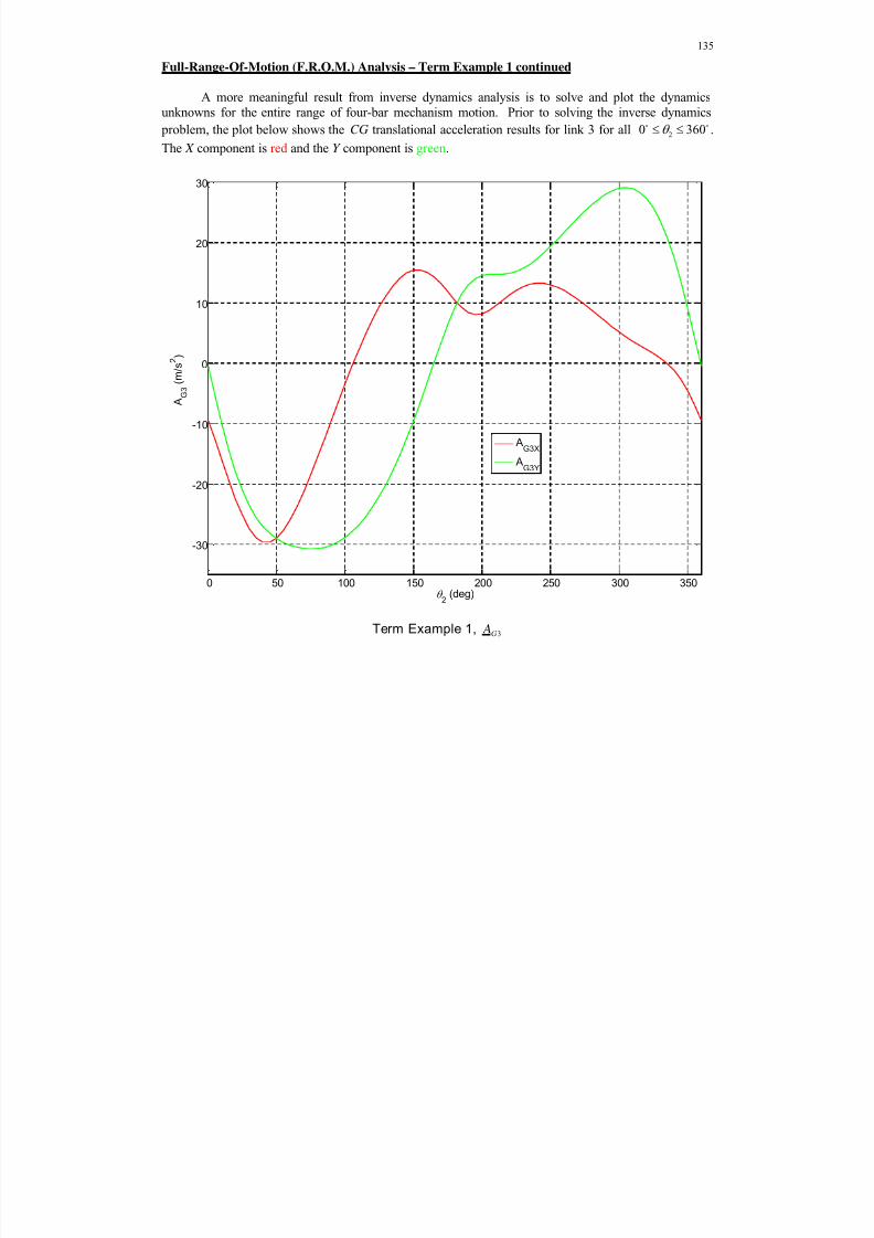
8/11/2019 Mechanism kinematics & dynamics.pdf
http://slidepdf.com/reader/full/mechanism-kinematics-dynamicspdf 135/269
135
Full-Range-Of-Motion (F.R.O.M.) Analysis – Term Example 1 continued
A more meaningful result from inverse dynamics analysis is to solve and plot the dynamicsunknowns for the entire range of four-bar mechanism motion. Prior to solving the inverse dynamics
problem, the plot below shows the CG translational acceleration results for link 3 for all 20 360 .
The X component is red and the Y component is green.
Term Example 1, 3G A
0 50 100 150 200 250 300 350
-30
-20
-10
0
10
20
30
2 (deg)
A G 3
( m / s
2 )
AG3X
AG3Y
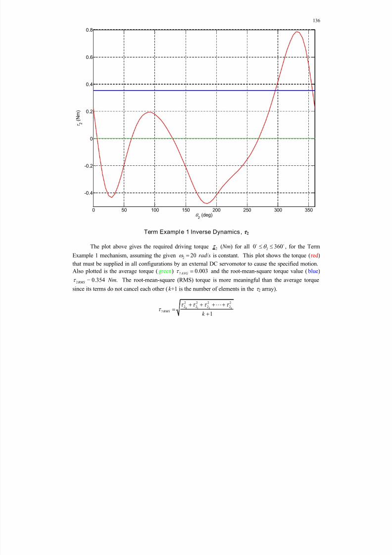
8/11/2019 Mechanism kinematics & dynamics.pdf
http://slidepdf.com/reader/full/mechanism-kinematics-dynamicspdf 136/269
136
Term Example 1 Inverse Dynamics, 2
The plot above gives the required driving torque 2 ( Nm) for all 20 360 , for the Term
Example 1 mechanism, assuming the given 2 20 rad /s is constant. This plot shows the torque (red )
that must be supplied in all configurations by an external DC servomotor to cause the specified motion.
Also plotted is the average torque (green) 2 0.003 AVG and the root-mean-square torque value ( blue)
2 0.354 RMS Nm. The root-mean-square (RMS) torque is more meaningful than the average torque
since its terms do not cancel each other (k +1 is the number of elements in the 2 array).
0 1 2
2 2 2 2
2 2 2 2
21
k
RMS k
0 50 100 150 200 250 300 350
-0.4
-0.2
0
0.2
0.4
0.6
0.8
2 (deg)
2
( N m )

8/11/2019 Mechanism kinematics & dynamics.pdf
http://slidepdf.com/reader/full/mechanism-kinematics-dynamicspdf 137/269
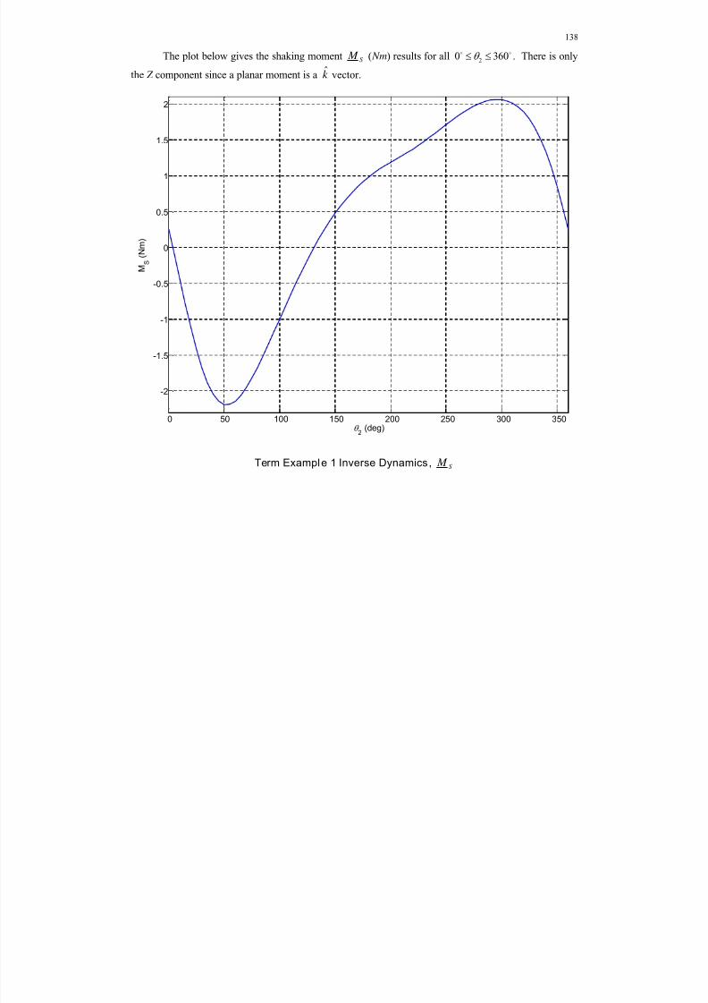
8/11/2019 Mechanism kinematics & dynamics.pdf
http://slidepdf.com/reader/full/mechanism-kinematics-dynamicspdf 138/269
138
The plot below gives the shaking moment S M ( Nm) results for all 20 360 . There is only
the Z component since a planar moment is a k vector.
Term Example 1 Inverse Dynamics, S M
0 50 100 150 200 250 300 350
-2
-1.5
-1
-0.5
0
0.5
1
1.5
2
2 (deg)
M
S
( N m )
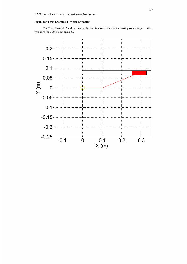
8/11/2019 Mechanism kinematics & dynamics.pdf
http://slidepdf.com/reader/full/mechanism-kinematics-dynamicspdf 139/269
139
3.9.3 Term Example 2: Slider-Crank Mechanism
Figure for Term Example 2 Inverse Dynamics
The Term Example 2 slider-crank mechanism is shown below at the starting (or ending) position,
with zero (or 360 ) input angle 2.
-0.1 0 0.1 0.2 0.3
-0.25
-0.2
-0.15
-0.1
-0.05
0
0.05
0.1
0.15
0.2
X (m)
Y ( m )

8/11/2019 Mechanism kinematics & dynamics.pdf
http://slidepdf.com/reader/full/mechanism-kinematics-dynamicspdf 140/269
140
Slider-crank mechanism inverse dynamics example – Term Example 2 continued
This is the mechanism from Term Example 2 (right branch), with kinematics solutions as
presented before. Given r 2 = 0.102, r 3 = 0.203, h = 0.076 m, 230 , 3
7.1 , x = 0.29 m, 2 15
rad /s (constant), 3 6.58 rad /s, 0.60 x m/s, 2 0 , 3 62.33 rad /s2, and 30.15 x m/s2.
All moving links are wood, with mass density 830.4 kg/m3. Links 2 and 3 have rectangular
dimensions r i x 0.019 x 0.013 thick (m; i=2,3); link 4 has rectangular dimensions 0.076 x 0.019 x 0.013thick (m), as shown on the previous page. The calculated inertia parameters are m2 = 0.020, m3 = 0.041,m4 = 0.015 (kg) and I G2 Z = 1.819e-005, I G3 Z = 1.418e-004 (kgm
2). The CGs all lie at their respective linkcenters. There is a constant external force of 1 N acting at the center of the piston end, directedhorizontally to the left; gravity is included but all other external forces and moments are zero. We
assume the coefficient of kinetic friction between the piston and the fixed wall is = 0.2.
Snapshot Analysis (one input angle)
At 2 30 , given this mechanism and motion, calculate the four vector internal joint forces, the
driving torque 2 , and the shaking force and moment ,S S F M for this instant (snapshot).
21
21
32
32
43
43
14
2
1 0 1 0 0 0 0 0 0.202
0 1 0 1 0 0 0 0 0.0
-0.025 0.044 -0.025 0.044 0 0 0 1
0 0 1 0 1 0 0 0
0 0 0 1 0 1 0 0
0 0 -0.013 0.101 -0.013 0.101 0 0
0 0 0 0 1 0 0.2 00 0 0 0 0 1 1 0
X
Y
X
Y
X
Y
Y
F
F
F
F
F
F
F
84
0
1.018
0.168
0.009
0.5400.150
The solution is accomplished by Gaussian elimination, or 1
v A b
, or by the reduced 5x5 plus
decoupled link 2 method (see the on-line ME 3011 NotesBook Supplement). All methods yield thesame results. Snapshot answers:
21
21
32
32
43
43
14
2
0.736
0.121
0.5340.037
0.484
0.131
0.281
0.039
X
Y
X
Y
X
Y
Y
F
F
F F
vF
F
F
( N , Nm)0.680
0.401S F
( N ) ˆ0.116S M k ( Nm)

8/11/2019 Mechanism kinematics & dynamics.pdf
http://slidepdf.com/reader/full/mechanism-kinematics-dynamicspdf 141/269
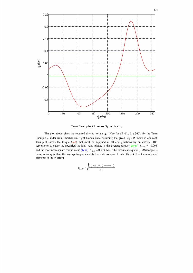
8/11/2019 Mechanism kinematics & dynamics.pdf
http://slidepdf.com/reader/full/mechanism-kinematics-dynamicspdf 142/269
142
Term Example 2 Inverse Dynamics, 2
The plot above gives the required driving torque 2 ( Nm) for all20 360 , for the Term
Example 2 slider-crank mechanism, right branch only, assuming the given 2 15 rad /s is constant.
This plot shows the torque (red ) that must be supplied in all configurations by an external DC
servomotor to cause the specified motion. Also plotted is the average torque (green) 2 0.004 AVG
and the root-mean-square torque value ( blue) 2 0.099 RMS Nm. The root-mean-square (RMS) torque is
more meaningful than the average torque since its terms do not cancel each other (k +1 is the number of
elements in the 2 array).
0 1 2
2 2 2 2
2 2 2 2
21
k
RMS k
0 50 100 150 200 250 300 350
-0.1
-0.05
0
0.05
0.1
0.15
0.2
0.25
2 (deg)
2
( N m )

8/11/2019 Mechanism kinematics & dynamics.pdf
http://slidepdf.com/reader/full/mechanism-kinematics-dynamicspdf 143/269
143
The plot below gives the shaking force S F ( N ) results for all 20 360 . The X component
is red and the Y component is green.
Term Example 2 Inverse Dynamics, S F
0 50 100 150 200 250 300 350-3
-2.5
-2
-1.5
-1
-0.5
0
0.5
1
.5
2 (deg)
F S
( N )
FSX
FSY
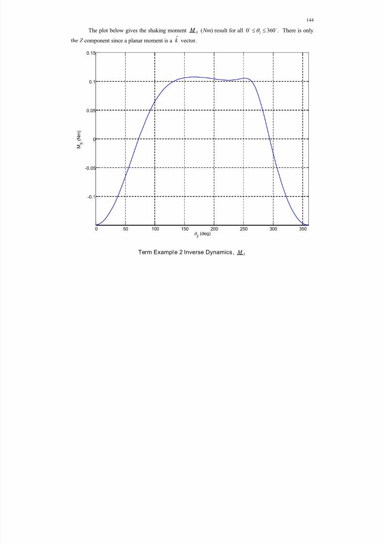
8/11/2019 Mechanism kinematics & dynamics.pdf
http://slidepdf.com/reader/full/mechanism-kinematics-dynamicspdf 144/269
144
The plot below gives the shaking moment S M ( Nm) result for all 20 360 . There is only
the Z component since a planar moment is a k vector.
Term Example 2 Inverse Dynamics, S M
0 50 100 150 200 250 300 350
-0.1
-0.05
0
0.05
0.1
0.15
2 (deg)
M
S
( N m )

8/11/2019 Mechanism kinematics & dynamics.pdf
http://slidepdf.com/reader/full/mechanism-kinematics-dynamicspdf 145/269
145
4. Gears and Cams
4.1 Gears
4.1.1 Gear Introduction
Gears are used to transfer motion between rotating shafts in machinery, mechanisms, robots,vehicles, toys, and other electromechanical systems. Gears cause changes in angular velocity, torque,and direction. Gears are used in various applications, from can openers to aircraft carriers. Belt andchain drives are related to gear mechanisms.
Robot joint example
Gear Classification
Externally-meshing Spur Gears Internally-meshing Spur Gears

8/11/2019 Mechanism kinematics & dynamics.pdf
http://slidepdf.com/reader/full/mechanism-kinematics-dynamicspdf 146/269
146
Helical (Parallel Shaft) Helical (Crossed Shaft)
Rack & Pinion Worm and Gear
Straight Bevel Gears Spiral Bevel Gears
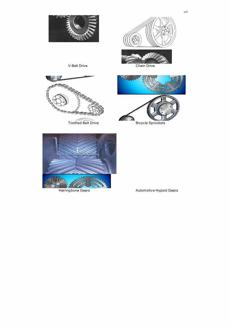
8/11/2019 Mechanism kinematics & dynamics.pdf
http://slidepdf.com/reader/full/mechanism-kinematics-dynamicspdf 147/269
147
V-Belt Drive Chain Drive
Toothed Belt Drive Bicycle Sprockets
Herringbone Gears Automotive Hypoid Gears

8/11/2019 Mechanism kinematics & dynamics.pdf
http://slidepdf.com/reader/full/mechanism-kinematics-dynamicspdf 148/269
148
Automotive Gear Train Automotive Differential
Planetary Gear Train Planetary Gear Train – Aircraft
Non-Circular Gears Harmonic Gearing

8/11/2019 Mechanism kinematics & dynamics.pdf
http://slidepdf.com/reader/full/mechanism-kinematics-dynamicspdf 149/269
149
Harmonic Gearing
“The harmonic gear allows high reduction ratios with concentric shafts and with very low
backlash and vibration. It is based on a very simple construction utilizing metal’s elasto-mechanical property.”
“Harmonic drive transmissions are noted for their ability to reduce backlash in a motion controlsystem. How they work is through the use of a thin-walled flexible cup with external splines on its lip,
placed inside a circular thick-walled rigid ring machined with internal splines. The external flexible
spline has two fewer teeth than the internal circular spline. An elliptical cam enclosed in an antifriction ball bearing assembly is mounted inside the flexible cup and forces the flexible cup splines to push
deeply into the rigid ring at two opposite points while rotating. The two contact points rotate at a speed
governed by the difference in the number of teeth on the two splines. This method basically preloadsthe teeth, which reduces backlash.”
roymech.co.uk
Harmonic Gear Sketch
roymech.co.uk
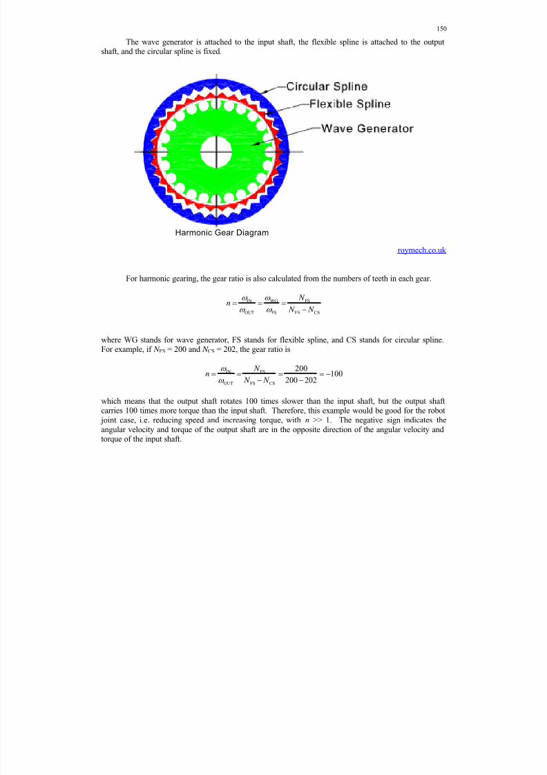
8/11/2019 Mechanism kinematics & dynamics.pdf
http://slidepdf.com/reader/full/mechanism-kinematics-dynamicspdf 150/269
150
The wave generator is attached to the input shaft, the flexible spline is attached to the outputshaft, and the circular spline is fixed.
Harmonic Gear Diagram
roymech.co.uk
For harmonic gearing, the gear ratio is also calculated from the numbers of teeth in each gear.
IN WG FS
OUT FS FS CS
N n
N N
where WG stands for wave generator, FS stands for flexible spline, and CS stands for circular spline.For example, if N FS = 200 and N CS = 202, the gear ratio is
IN FS
OUT FS CS
200100
200 202
N n
N N
which means that the output shaft rotates 100 times slower than the input shaft, but the output shaftcarries 100 times more torque than the input shaft. Therefore, this example would be good for the robot
joint case, i.e. reducing speed and increasing torque, with n >> 1. The negative sign indicates theangular velocity and torque of the output shaft are in the opposite direction of the angular velocity andtorque of the input shaft.
8/11/2019 Mechanism kinematics & dynamics.pdf
http://slidepdf.com/reader/full/mechanism-kinematics-dynamicspdf 151/269
151
4.1.2 Gear Ratio
Classification of gear ratios
If 1n 2 1
2 1
The output has reduced speed and increased torque.
This is the electric motor / robot joint case, where n >> 1.
If 1n 2 1
2 1
The output has increased speed and reduced torque.
This is the bicycle transmission case, except for some granny gears where n can be ashigh as 1.5.
If 1n 2 1
2 1
This case is called an idler, where the output speed and torque are unchanged, but thedirection reverses (for external spur gears)
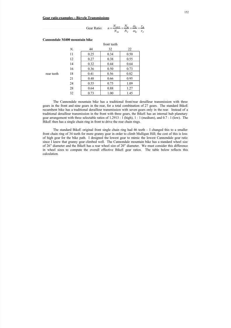
8/11/2019 Mechanism kinematics & dynamics.pdf
http://slidepdf.com/reader/full/mechanism-kinematics-dynamicspdf 152/269

8/11/2019 Mechanism kinematics & dynamics.pdf
http://slidepdf.com/reader/full/mechanism-kinematics-dynamicspdf 153/269
153
BikeE standard recumbent bike
front teeth
34 34 34
N i 1.2913 : 1 1 : 1 0.7 : 1
11 0.33 0.42 0.60
13 0.38 0.50 0.71
15 0.44 0.57 0.82
rear teeth 18 0.53 0.69 0.98
21 0.62 0.80 1.15
24 0.71 0.92 1.31
28 0.83 1.07 1.53
I was able to obtain a used deluxe BikeE recumbent bike from noted luthier Dan Erlewine. Idecided to keep the front chain ring of 46 teeth (numbers of teeth in the rear chain ring and the planetary
gear ratios in the rear hub are identical between the standard and deluxe BikeE models). This means mynew deluxe BikeE doesn’t climb as well as my modified standard BikeE, but it flies much faster on the bike path in high gear than the standard BikeE! Again, the difference in wheel diameter is taken intoaccount in the table below.
BikeE deluxe recumbent bike
front teeth
46 46 46
N i 1.2913 1 0.7
11 0.24 0.31 0.44
13 0.28 0.37 0.52
15 0.33 0.42 0.61
rear teeth 18 0.39 0.51 0.73
21 0.46 0.59 0.85
24 0.53 0.68 0.97
28 0.61 0.79 1.13
We see that the standard BikeE that was designed to equal the granny gear of the Cannondale (itwas exceeded, 1.53 vs. 1.45). However, the mountain bike still climbs better in granny gear, since your
legs are positioned above the pedals in the mountain bike case, and your legs are positioned straight outin front of you in the recumbent bike case.
Unlike the robot joint example, bicycle gearing generally has n < 1 and so the transmission
increases angular velocity
decreases torque by the gear ratio n. The exception is the granny gears with n > 1.

8/11/2019 Mechanism kinematics & dynamics.pdf
http://slidepdf.com/reader/full/mechanism-kinematics-dynamicspdf 154/269
154
4.1.3 Gear Trains
To obtain a higher gear ratio than practical with a single pair of standard involute spur gears, onecan mate any number of spur gears in a gearbox, or gear train. The leftmost gear is the driving gear andthe rightmost is the output gear. All intermediate gears are first the driven gear and then the driving gearas we proceed from left to right. Let us calculate the overall gear ratio nGT .
IN GT
OUT n
Example
We can find the overall gear ratio by canceling neighboring intermediate angular velocities.
Each term in the above product may be replaced by its known number of teeth ratio.
All intermediate ratios cancel, so
We could have done the same with pitch radii instead of number of teeth because they are in direct proportion.
So, the intermediate gears are idlers. Their number of teeth effect cancels out, but they do changedirection. We should have included the +/– signs, by inspection. For gear trains composed ofexternally-meshing spur gear pairs:
odd number of gears the output is in the same direction as the inputeven number of gears the output is in the opposite direction as the input
8/11/2019 Mechanism kinematics & dynamics.pdf
http://slidepdf.com/reader/full/mechanism-kinematics-dynamicspdf 155/269
155
Improved gear train
That gear train concept did not work. Now let us mate any number of spur gears, where thedriving and driven gears are distinct, because each pair is rigidly attached to the same shaft. Again, letus calculate the overall gear ratio.
IN GT
OUT
n
Example
Again, we use the equation
But now the gears rigidly attached to the same shaft have the same angular velocity ratio, so
The general formula for this case is
Again, we must consider direction
For gear trains composed of externally-meshing spur gear pairs:odd number of pairs the output is in the opposite direction as the inputeven number of pairs the output is in the same direction as the input
8/11/2019 Mechanism kinematics & dynamics.pdf
http://slidepdf.com/reader/full/mechanism-kinematics-dynamicspdf 156/269
156
4.1.4 Involute Spur Gear Standardization
Rolling Cylinders
Mating spur gears are based on two pitch circles rolling without slip. These are fictitious circles,i.e. you cannot look on a gear to see them. The actual gear teeth both roll and slide with respect to eachother (via the two-dof gear joint).
Fundamental Law of Gearing
The angular velocity between the gears of a gearset must remain constant throughout the mesh .
From our study of linkage velocity, we know this is no easy feat. Velocity ratios in a linkagevary wildly over the range of motion.
Velocity Ratio1
VR OUT IN
IN OUT
r
r n
Torque Ratio TR IN OUT
OUT IN
r n
r
The velocity ratio is the inverse of the gear ratio n and the torque ratio is the same as the gearratio n defined previously. The torque ratio is also called Mechanical Advantage (MA).
Involute Function
Standard spur gears have an involute tooth shape. If the gears’ center distance is not perfect(tolerances, thermal expansion, wear – in design the center distance is increased slightly by the engineerto allow for these effects; this is called clearance), the angular velocity ratio will still be constant tosatisfy the Fundamental Law of Gearing.
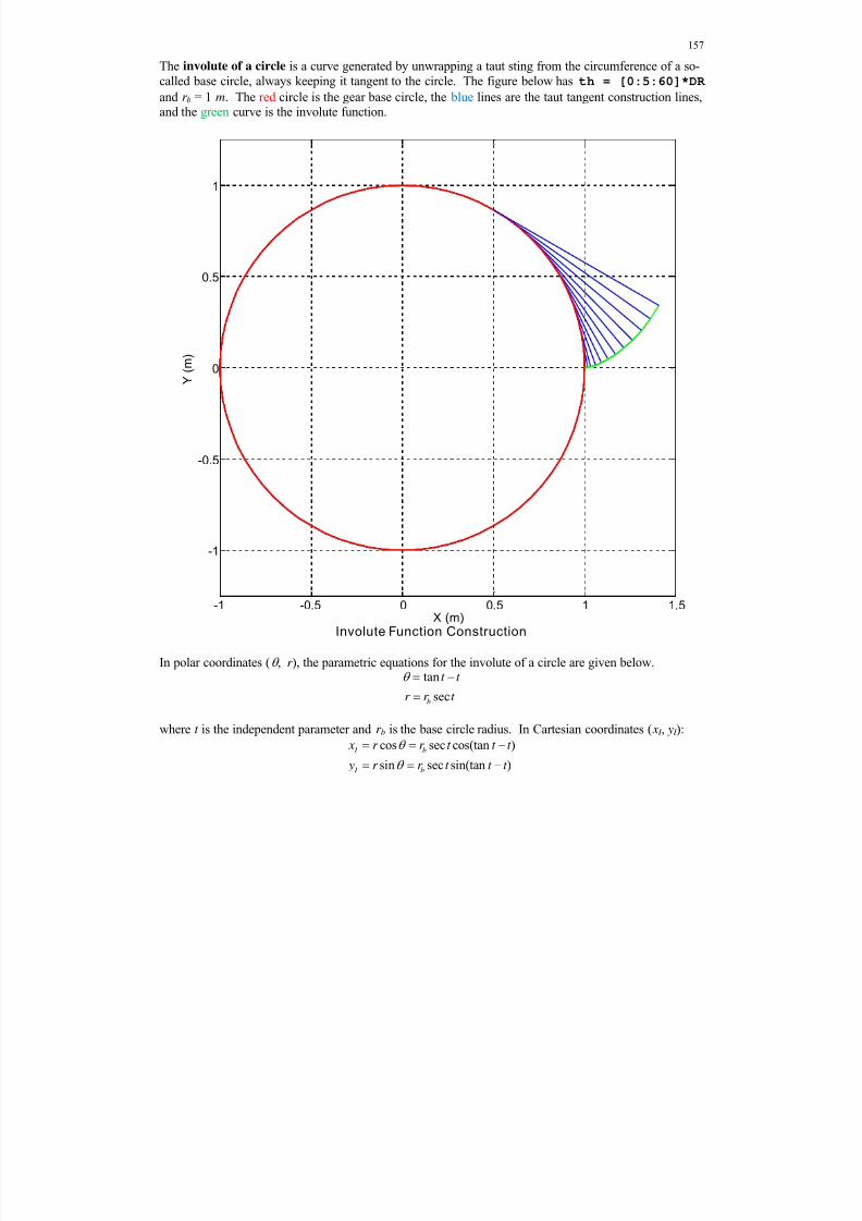
8/11/2019 Mechanism kinematics & dynamics.pdf
http://slidepdf.com/reader/full/mechanism-kinematics-dynamicspdf 157/269
157
The involute of a circle is a curve generated by unwrapping a taut sting from the circumference of a so-called base circle, always keeping it tangent to the circle. The figure below has th = [0:5:60]*DR
and r b = 1 m. The red circle is the gear base circle, the blue lines are the taut tangent construction lines,and the green curve is the involute function.
Involute Function Construction
In polar coordinates ( , r ), the parametric equations for the involute of a circle are given below.tan
secb
t t
r r t
where t is the independent parameter and r b is the base circle radius. In Cartesian coordinates ( x I , y I ):
cos sec cos(tan )
sin sec sin(tan )
I b
I b
x r r t t t
y r r t t t
-1 -0.5 0 0.5 1 1.5
-1
-0.5
0
0.5
1
X (m)
Y ( m )
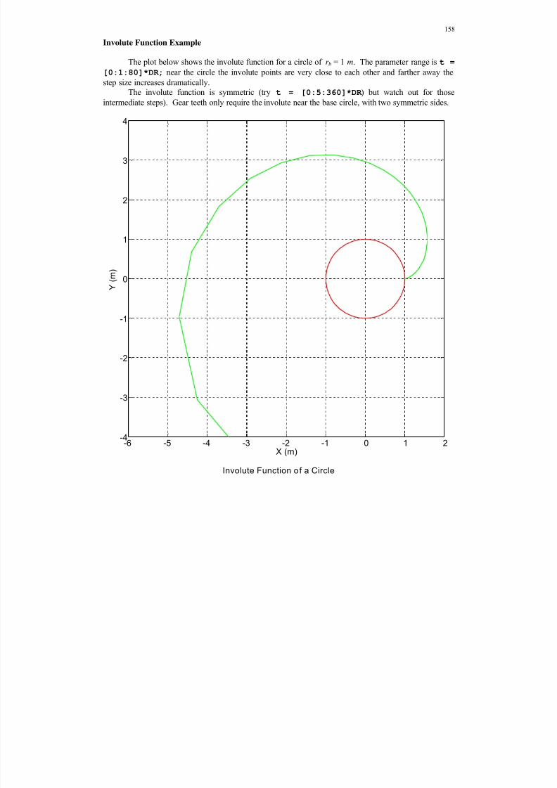
8/11/2019 Mechanism kinematics & dynamics.pdf
http://slidepdf.com/reader/full/mechanism-kinematics-dynamicspdf 158/269
158
Involute Function Example
The plot below shows the involute function for a circle of r b = 1 m. The parameter range is t =
[0:1:80]*DR; near the circle the involute points are very close to each other and farther away the
step size increases dramatically.The involute function is symmetric (try t = [0:5:360]*DR ) but watch out for those
intermediate steps). Gear teeth only require the involute near the base circle, with two symmetric sides.
Involute Function of a Circle
-6 -5 -4 -3 -2 -1 0 1 2-4
-3
-2
-1
0
1
2
3
4
X (m)
Y ( m )

8/11/2019 Mechanism kinematics & dynamics.pdf
http://slidepdf.com/reader/full/mechanism-kinematics-dynamicspdf 159/269

8/11/2019 Mechanism kinematics & dynamics.pdf
http://slidepdf.com/reader/full/mechanism-kinematics-dynamicspdf 160/269
160
Norton (2008)
The length of contact is measured along the axis of transmission. The beginning of contact iswhen the tip of the driven gear tooth intersects the axis of transmission. The end of contact is when thetip of driving gear tooth intersects the axis of transmission, as shown in the figure above. Only one ortwo teeth are in contact at any one time for standard spur gears.
For harmonic gearing, many teeth are in contact at any one time, which provides a higher gearratio in a smaller package.
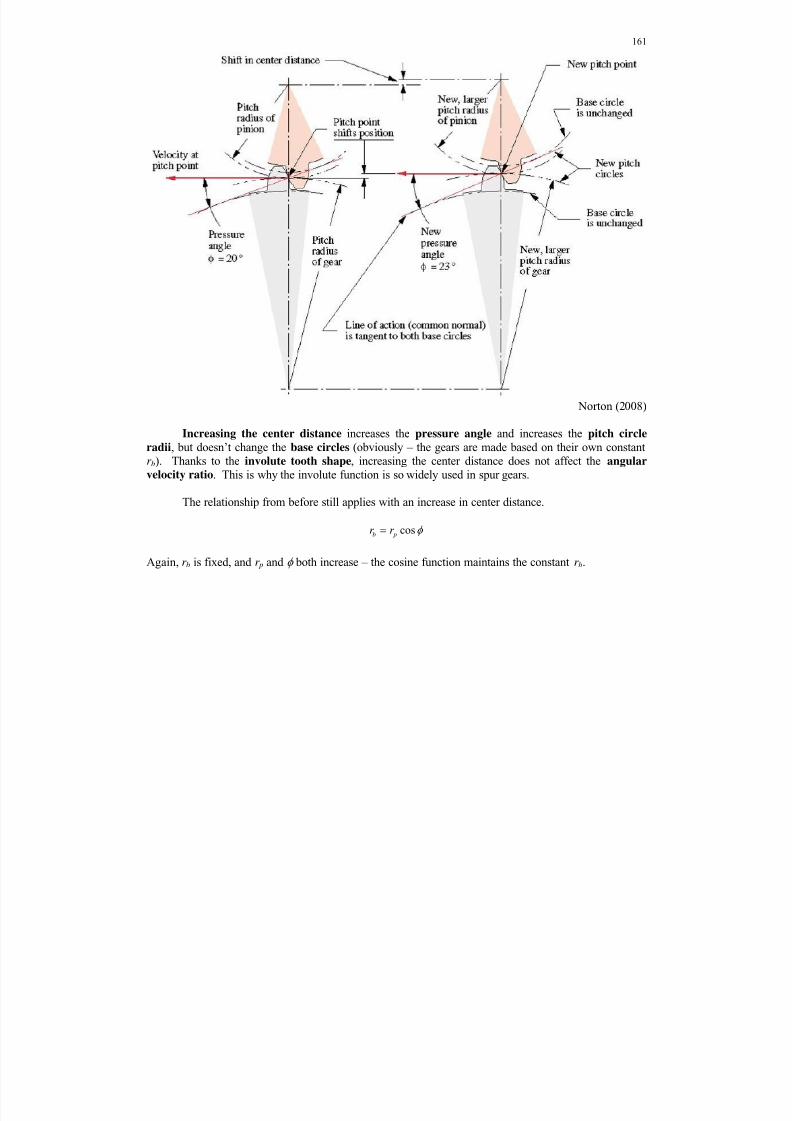
8/11/2019 Mechanism kinematics & dynamics.pdf
http://slidepdf.com/reader/full/mechanism-kinematics-dynamicspdf 161/269
161
Norton (2008)
Increasing the center distance increases the pressure angle and increases the pitch circle
radii, but doesn’t change the base circles (obviously – the gears are made based on their own constantr b). Thanks to the involute tooth shape, increasing the center distance does not affect the angular
velocity ratio. This is why the involute function is so widely used in spur gears.
The relationship from before still applies with an increase in center distance.
cosb pr r
Again, r b is fixed, and r p and both increase – the cosine function maintains the constant r b.
8/11/2019 Mechanism kinematics & dynamics.pdf
http://slidepdf.com/reader/full/mechanism-kinematics-dynamicspdf 162/269
162
Spur Gear Standardization
Gear standardization is used to allow interchangeability in manufacturing and to allow meshingof different size gears (different pitch radii and number of teeth) to achieve desired gear ratios. For twospur gears to mesh, they must have
1) the same pressure angle (see previous figures and definition)
2) the same diametral pitch (see the equation below)
3) standard tooth proportions (see the figure below)
diametral pitch d
N p
d
Where N is the number of teeth and d is the pitch diameter, both for each gear.
module1
d
d m
N p
Module is the SI version of diametral pitch (it is the inverse). SI gears are notinterchangeable with English system gears because of different tooth proportionstandards.
circular pitch c
d
p N
Circular pitch is the circumferential distance (arc length) between teeth along the pitchcircle of a spur gear.

8/11/2019 Mechanism kinematics & dynamics.pdf
http://slidepdf.com/reader/full/mechanism-kinematics-dynamicspdf 163/269
163
from Norton (2008)
Standard involute tooth proportions
Addendum is radial distance from pitch circle to top land of tooth.
Dedendum is radial distance from pitch circle to bottom land of tooth (not to the base circle).
Clearance is radial distance from bottom land to mating gear top land (radial backlash).
Face width is thickness of tooth and gear (mating widths needn’t be the same).
Tooth thickness t is the circumferential arc length of each tooth. It is related to the circular
pitch pc and backlash (next page) b by
2c p t b
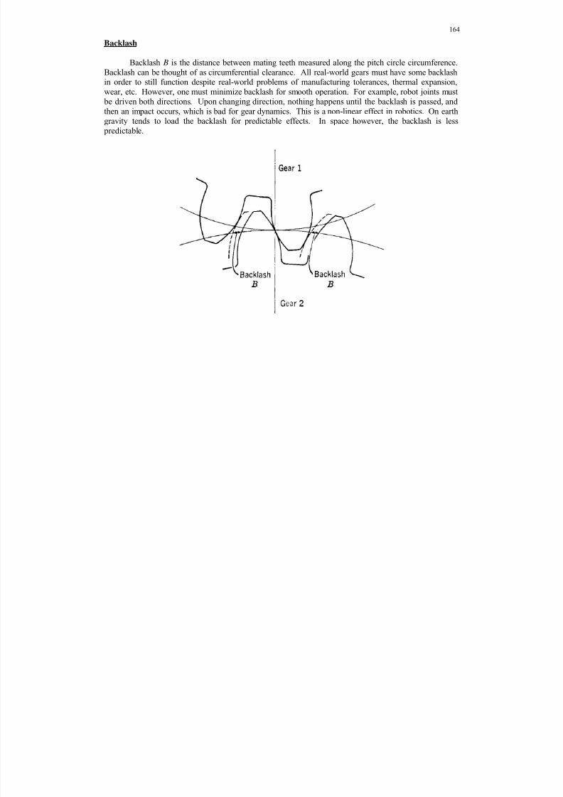
8/11/2019 Mechanism kinematics & dynamics.pdf
http://slidepdf.com/reader/full/mechanism-kinematics-dynamicspdf 164/269
164
Backlash
Backlash B is the distance between mating teeth measured along the pitch circle circumference.Backlash can be thought of as circumferential clearance. All real-world gears must have some backlashin order to still function despite real-world problems of manufacturing tolerances, thermal expansion,wear, etc. However, one must minimize backlash for smooth operation. For example, robot joints must be driven both directions. Upon changing direction, nothing happens until the backlash is passed, andthen an impact occurs, which is bad for gear dynamics. This is a non-linear effect in robotics. On earthgravity tends to load the backlash for predictable effects. In space however, the backlash is less predictable.

8/11/2019 Mechanism kinematics & dynamics.pdf
http://slidepdf.com/reader/full/mechanism-kinematics-dynamicspdf 165/269
165
4.1.5 Planetary Gear Trains
Planetary gear trains are also called epicyclic gear trains. The sun gear rotates about a fixed axis.Each planet gear rotates about its own axis and also orbits the sun gear. This happens with directmeshing of teeth, unlike celestial planetary motion. The arm link (which is a rigid body with no teeth)carries the planet(s) around the sun. The arm has a revolute joint to the sun gear on one side and anotherrevolute joint to the planet gear(s) on the other side. Planetary gear trains have two-dof, so two inputsmust be given to control the mechanism. For instance, one can drive the sun gear and the arm link withindependent external motors. Alternatively, the sun gear may be fixed and the arm link driven. Using planetary gear trains, one can obtain a higher gear ratio in a smaller package, compared to non-planetarygear trains.
Conventional Gear Pair Planetary Gear Train
3(3 1) 2(2) 1(1) 1 M 3(4 1) 2(3) 1(1) 2 M
IN OUT OUT
OUT IN IN
r N n
r N
? IN
OUT
n
We present the tabular method below to determine the gear ratio for various planetary gear trains.
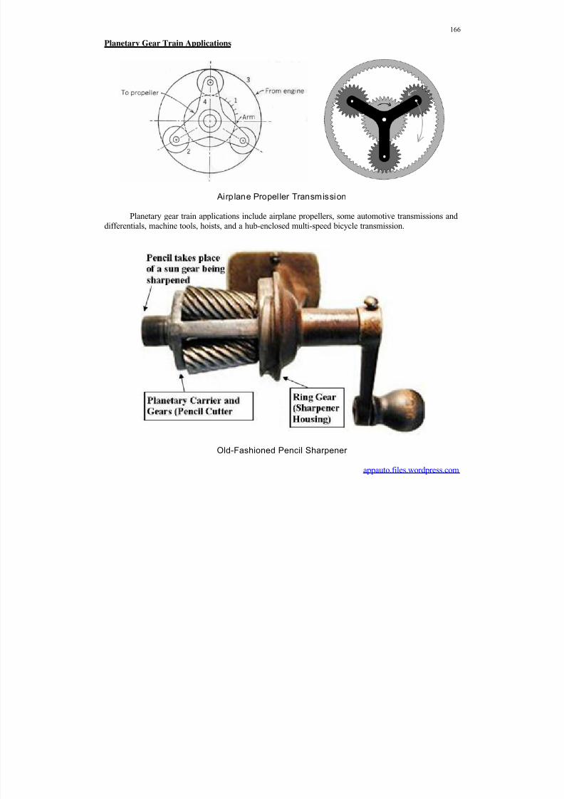
8/11/2019 Mechanism kinematics & dynamics.pdf
http://slidepdf.com/reader/full/mechanism-kinematics-dynamicspdf 166/269
166
Planetary Gear Train Applications
Airp lane Propel ler Transmission
Planetary gear train applications include airplane propellers, some automotive transmissions anddifferentials, machine tools, hoists, and a hub-enclosed multi-speed bicycle transmission.
Old-Fashioned Pencil Sharpener
appauto.files.wordpress.com
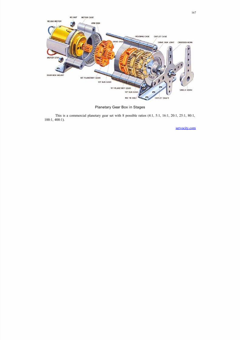
8/11/2019 Mechanism kinematics & dynamics.pdf
http://slidepdf.com/reader/full/mechanism-kinematics-dynamicspdf 167/269
167
Planetary Gear Box in Stages
This is a commercial planetary gear set with 8 possible ratios (4:1, 5:1, 16:1, 20:1, 25:1, 80:1,100:1, 400:1).
servocity.com
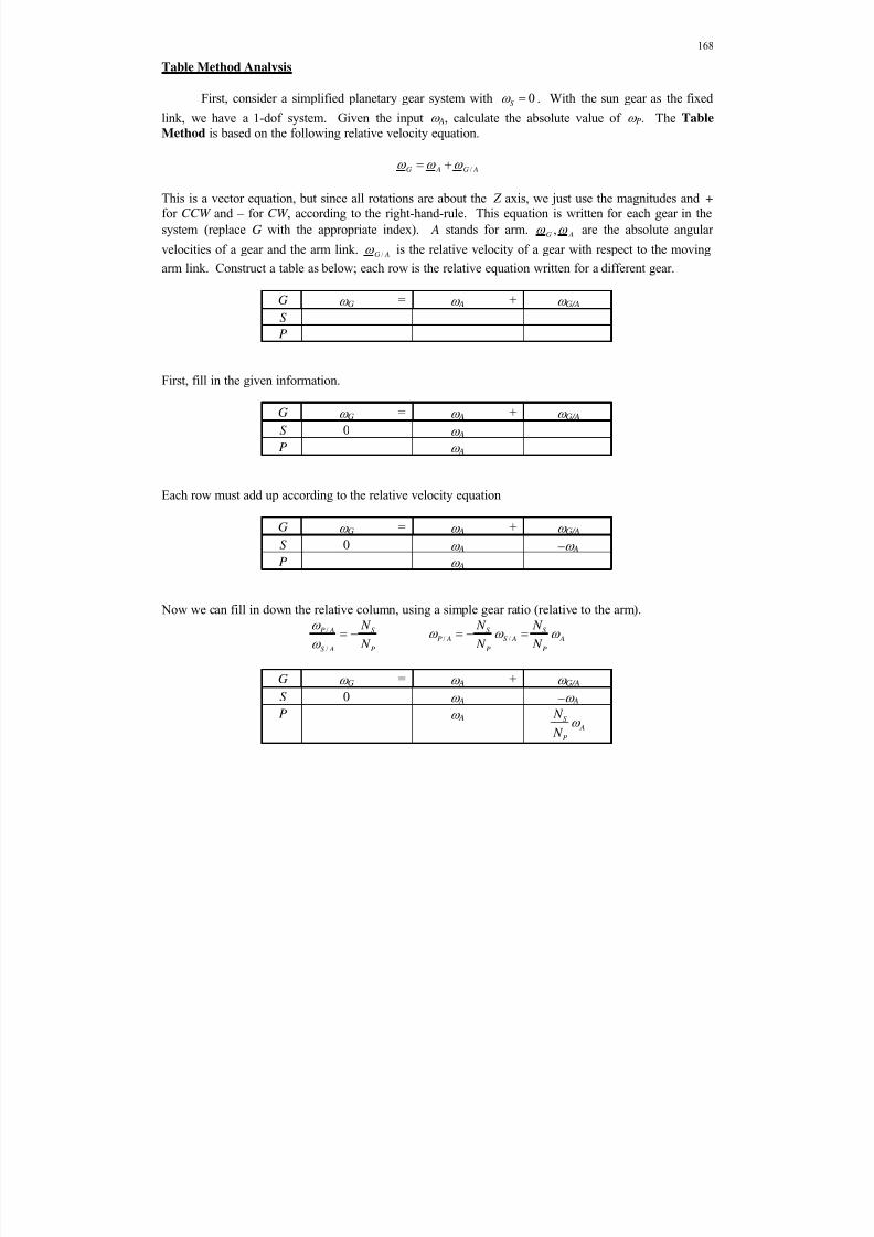
8/11/2019 Mechanism kinematics & dynamics.pdf
http://slidepdf.com/reader/full/mechanism-kinematics-dynamicspdf 168/269
168
Table Method Analysis
First, consider a simplified planetary gear system with 0S . With the sun gear as the fixed
link, we have a 1-dof system. Given the input A, calculate the absolute value of P. The Table
Method is based on the following relative velocity equation.
/G A G A
This is a vector equation, but since all rotations are about the Z axis, we just use the magnitudes and + for CCW and – for CW , according to the right-hand-rule. This equation is written for each gear in the
system (replace G with the appropriate index). A stands for arm. ,G A are the absolute angular
velocities of a gear and the arm link. /G A is the relative velocity of a gear with respect to the moving
arm link. Construct a table as below; each row is the relative equation written for a different gear.
G G = A + G/A
S
P
First, fill in the given information.
G G = A + G/A
S 0 A
P A
Each row must add up according to the relative velocity equation
G G = A + G/A
S 0 A – A
P A
Now we can fill in down the relative column, using a simple gear ratio (relative to the arm).
/
/
P A S
S A P
N
N
/ /
S S P A S A A
P P
N N
N N
G G = A + G/A
S 0 A – A
P A S A
P
N
N
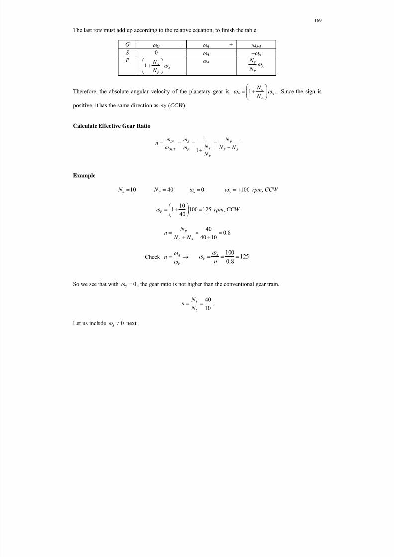
8/11/2019 Mechanism kinematics & dynamics.pdf
http://slidepdf.com/reader/full/mechanism-kinematics-dynamicspdf 169/269
169
The last row must add up according to the relative equation, to finish the table.
G G = A + G/A
S 0 A – A
P1 S
A
P
N
N
A S A
P
N
N
Therefore, the absolute angular velocity of the planetary gear is 1 S P A
P
N
N
. Since the sign is
positive, it has the same direction as A (CCW ).
Calculate Effective Gear Ratio
1
1
IN A P
S OUT P P S
P
N n
N N N
N
Example
10S N 40P
N 0S 100 A
rpm, CCW
101 100 125
40P
rpm, CCW
400.8
40 10P
P S
N n
N N
Check A
P
n
100125
0.8 A
Pn
So we see that with 0S , the gear ratio is not higher than the conventional gear train.
4010
P
S
N n N
.
Let us include 0S next.
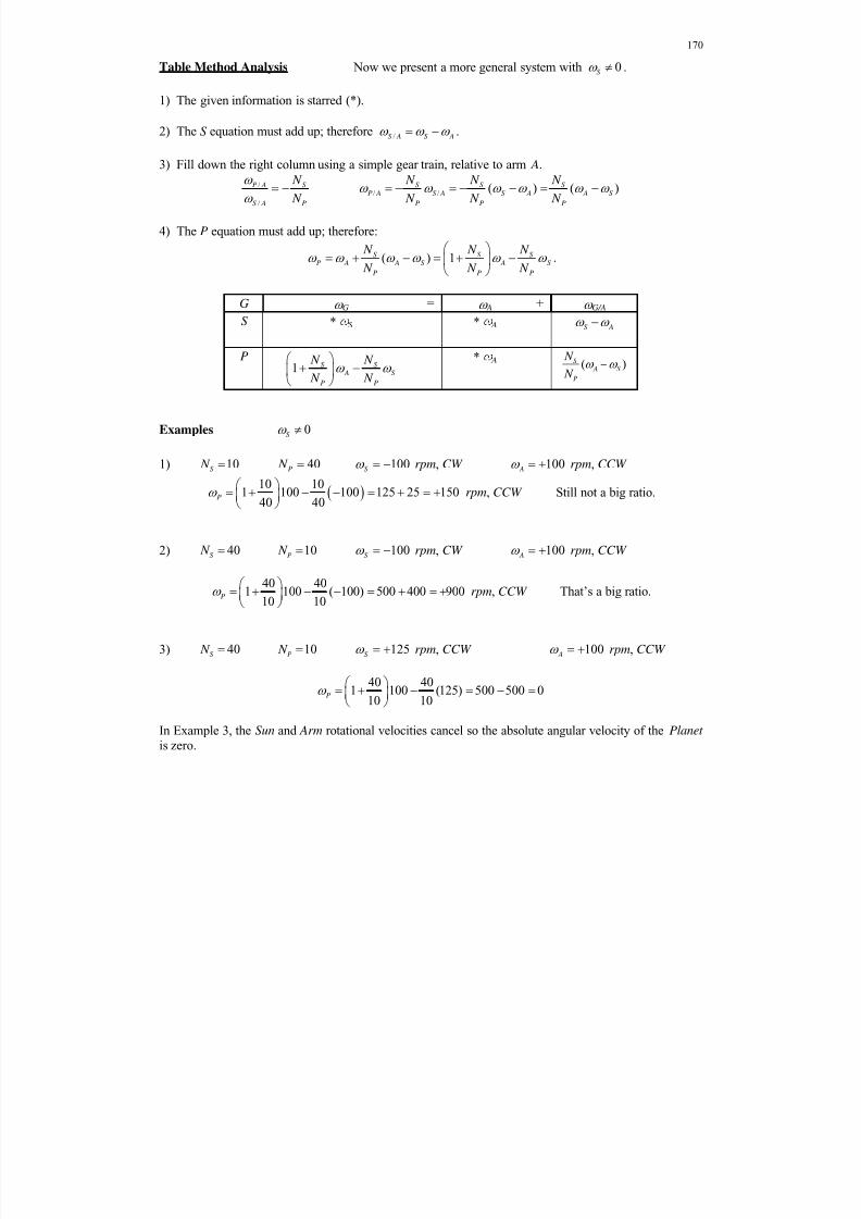
8/11/2019 Mechanism kinematics & dynamics.pdf
http://slidepdf.com/reader/full/mechanism-kinematics-dynamicspdf 170/269
170
Table Method Analysis Now we present a more general system with 0S .
1) The given information is starred (*).
2) The S equation must add up; therefore /S A S A .
3) Fill down the right column using a simple gear train, relative to arm A./
/
P A S
S A P
N
N
/ / ( ) ( )S S S
P A S A S A A S
P P P
N N N
N N N
4) The P equation must add up; therefore:
( ) 1S S S P A A S A S
P P P
N N N
N N N
.
G G = A + G/A
S * S * A S A
P1 S S
A S
P P
N N
N N
* A ( )S
A S
P
N
N
Examples 0S
1) 10S N 40P N 100S rpm, CW 100 A rpm, CCW
10 10
1 100 100 125 25 15040 40P
rpm, CCW Still not a big ratio.
2) 40S N 10P
N 100S rpm, CW 100 A rpm, CCW
40 401 100 ( 100) 500 400 900
10 10P
rpm, CCW That’s a big ratio.
3) 40S N 10P N 125S rpm, CCW 100 A rpm, CCW
40 401 100 (125) 500 500 0
10 10P
In Example 3, the Sun and Arm rotational velocities cancel so the absolute angular velocity of the Planet is zero.

8/11/2019 Mechanism kinematics & dynamics.pdf
http://slidepdf.com/reader/full/mechanism-kinematics-dynamicspdf 171/269
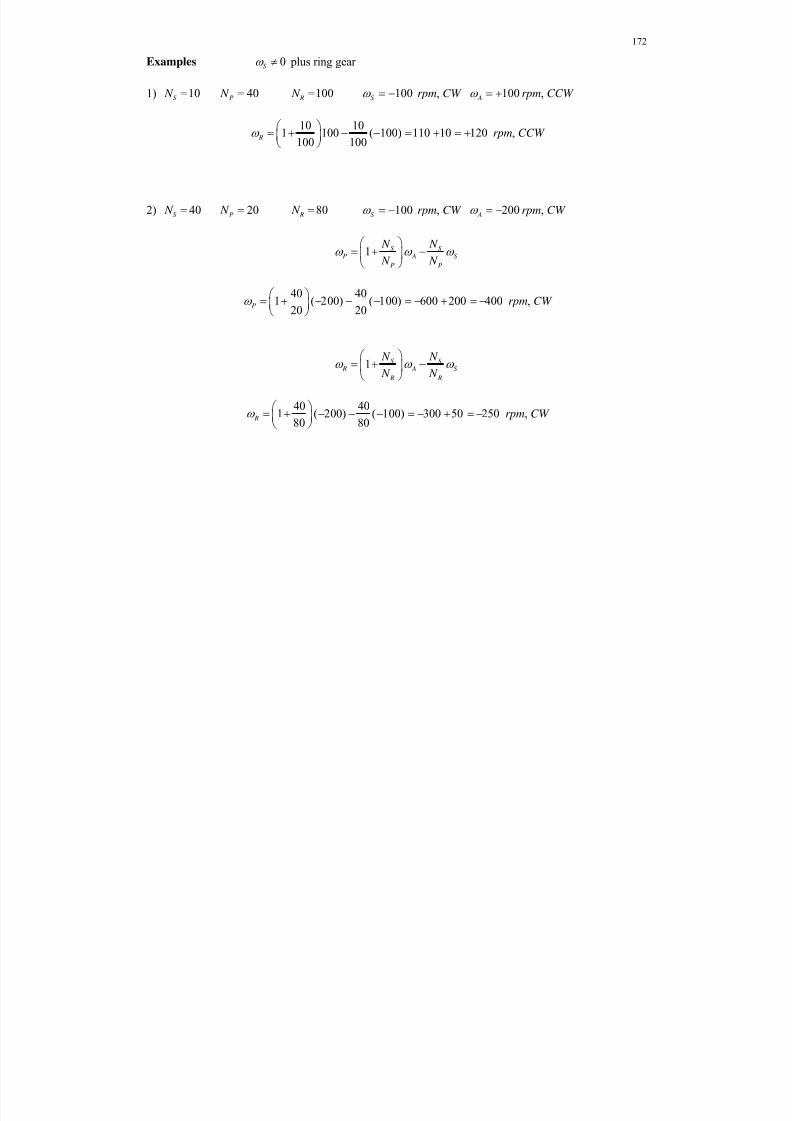
8/11/2019 Mechanism kinematics & dynamics.pdf
http://slidepdf.com/reader/full/mechanism-kinematics-dynamicspdf 172/269
172
Examples 0S plus ring gear
1) 10S N 40P N 100 R N 100S rpm, CW 100 A rpm, CCW
10 101 100 ( 100) 110 10 120
100 100 R
rpm, CCW
2) 40S N 20P
N 80 R N 100S
rpm, CW 200 A rpm, CW
1 S S P A S
P P
N N
N N
40 40
1 ( 200) ( 100) 600 200 40020 20P
rpm, CW
1 S S R A S
R R
N N
N N
40 401 ( 200) ( 100) 300 50 250
80 80 R
rpm, CW

8/11/2019 Mechanism kinematics & dynamics.pdf
http://slidepdf.com/reader/full/mechanism-kinematics-dynamicspdf 173/269
173
4.2 Cams
4.2.1 Cam Introduction
Applications
Compared to linkages, it is easier to design desired motion with cams, but it is more expensive anddifficult to produce. Also, the cam contact and wear properties are worse than for linkages.
Cam Classification
Mabie & Reinholtz (19874
)
a) disk cam with knife-edgefollower
b) disk cam with radial rollerfollower
c) disk cam with offset radialroller follower
d) disk cam with oscillatingroller follower
e) disk cam with radial flat-facedfollower
f) disk cam with oscillating flat-faced follower
4 H.H. Mabie and C.F. Reinholtz, 1987, Mechanisms and Dynamics of Machinery, Wiley.
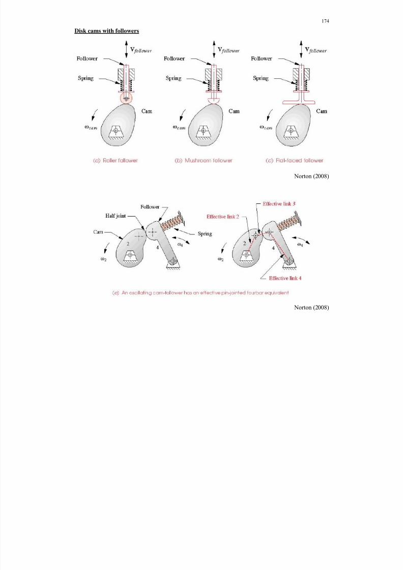
8/11/2019 Mechanism kinematics & dynamics.pdf
http://slidepdf.com/reader/full/mechanism-kinematics-dynamicspdf 174/269
174
Disk cams with followers
Norton (2008)
Norton (2008)
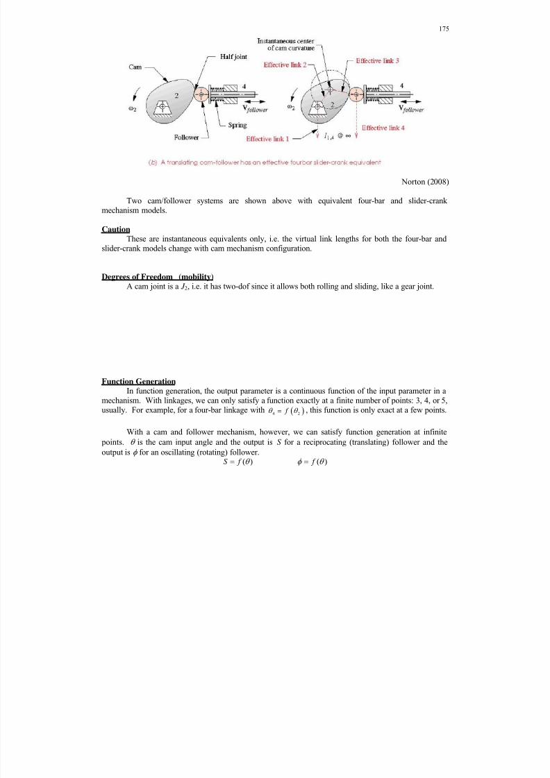
8/11/2019 Mechanism kinematics & dynamics.pdf
http://slidepdf.com/reader/full/mechanism-kinematics-dynamicspdf 175/269
175
Norton (2008)
Two cam/follower systems are shown above with equivalent four-bar and slider-crank
mechanism models.
Caution These are instantaneous equivalents only, i.e. the virtual link lengths for both the four-bar and
slider-crank models change with cam mechanism configuration.
Degrees of Freedom (mobility)
A cam joint is a J 2, i.e. it has two-dof since it allows both rolling and sliding, like a gear joint.
Function Generation
In function generation, the output parameter is a continuous function of the input parameter in amechanism. With linkages, we can only satisfy a function exactly at a finite number of points: 3, 4, or 5,usually. For example, for a four-bar linkage with 4 2 f , this function is only exact at a few points.
With a cam and follower mechanism, however, we can satisfy function generation at infinite
points. is the cam input angle and the output is S for a reciprocating (translating) follower and the
output is for an oscillating (rotating) follower.( )S f ( ) f
8/11/2019 Mechanism kinematics & dynamics.pdf
http://slidepdf.com/reader/full/mechanism-kinematics-dynamicspdf 176/269
8/11/2019 Mechanism kinematics & dynamics.pdf
http://slidepdf.com/reader/full/mechanism-kinematics-dynamicspdf 177/269
177
S V A J Diagrams
In cam synthesis (design), we are only given the total motion range and perhaps some timingrequirements. It is the engineer’s job to determine the position curves and to match the velocity andacceleration across junctions. Position is automatically matched by shifting the dependent functionaxes. Draw S V A J diagrams vs. time to graphically see if the Fundamental Law of Cam Design is
satisfied for candidate curves. We can plot vs. time or vs. input cam angle (assuming constant angularvelocity, t ).
The slope of a function is the value of its derivative at a point in time (or ). Therefore, forcontinuous velocity and acceleration curves, the slopes of the position and velocity curves must matchacross all junctions. The slope of the acceleration can be discontinuous (leading to finite jumps in jerk), but the acceleration itself must be continuous.
Cam motion curves are very much like the input link motion curves discussed earlier, for inputlinks that start and stop at zero velocity and acceleration. In fact, I adapted the input motion curves fromcam motion curve design.
Generic Cam-Follower Motion Profile Figure
Define each separate function so the value is zero at the initial angle, which is zero. Then to put the
whole cam motion profile together, just shift the and S axes.
Match S easy, just shift the S axis.
Match V slope of S must match across junctions.
1 1( ) ( 0)i i i i i
v v
apply to all functions / junctions.
Match A slope of V must match across junctions.
1 1( ) ( 0)i i i i i
a a
apply to all functions / junctions.
8/11/2019 Mechanism kinematics & dynamics.pdf
http://slidepdf.com/reader/full/mechanism-kinematics-dynamicspdf 178/269
178
Cam Follower Motion Profile Examples Example 1
rise – dwell portion. Specify parabolic (constant acceleration) to straight line (constant velocity) rise,followed by a dwell.
parabolic function constant velocity function dwell
S: 2
1 1 0 1
1( )
2 f A
2 2 0 2( ) f V 3 3( ) 0 f
V: 1 1 0 1( )v A
2 2 0( )v V 3 3( ) 0v
A: 1 1 0( )a A
2 2( ) 0a 3 3( ) 0a
J: 1 1( ) 0 j
2 2( ) 0 j 3 3( ) 0 j
Match S at junction B just shift the vertical axis up.
Match V at junction B
1 1 1 2 2( ) ( 0)v v 0 1 0 A V so 0 0 1V A
Try to match A at junction B:
1 1 1 2 2( ) ( 0)a a 0 0 A
0 0 A is impossible, or else the parabola is degenerate, which we cannot allow. This case violates the
Fundamental Law of Cam Design since the acceleration function cannot be made to be continuous at junction B. Therefore, this cam motion profile example cannot be used for cam design.
We have a bigger problem at junction C , between functions 2 and 3: the velocity function cannot be made to be continuous at junction C . Discontinuous velocity is one level worse than discontinuous
acceleration; either renders the resulting cam motion profile unacceptable.
Example 1 Plots

8/11/2019 Mechanism kinematics & dynamics.pdf
http://slidepdf.com/reader/full/mechanism-kinematics-dynamicspdf 179/269
179
Cam Follower Motion Profile Examples Example 2 Let us fix the rise portion only, at junction B. Then the problem at junction C can be fixed using
symmetry. We specify a half-cycloidal function (sinusoidal in cam angle) to a straight line (constantvelocity) rise.
half-cycloidal function constant velocity function
S 1 11 1 1
1 1
1( ) sin f L
2 2 0 2( ) f V
V 1 11 1
1 1
( ) 1 cos L
v
2 2 0( )v V
A 1 11 1 2
1 1
( ) sin L
a
2 2( ) 0a
J 2
1 11 1 3
1 1
( ) cos L
j
2 2( ) 0 j
Match S at junction B just shift the vertical axis up
Match V at junction B
1 1 1 2 2( ) ( 0)v v 1 10
1 1
1 cos L
V
so 1
0
1
2 LV
Match A at junction B
1 1 1 2 2( ) ( 0)a a 1 1
2
1 1
sin 0 L
0 = 0
In this case the acceleration function is continuous because the half-cycloidal function ensuresthat the acceleration is zero at the end of the function range. This case obeys the Fundamental Law of
Cam Design and so this cam motion profile example portion can be used for cam design.
Half-Cycloidal Rise (to connect with constant velocity)
0 20 40 60 800
1
2
S ( m )
Half Cycloid
0 20 40 60 800
0.05
V ( m / d e g )
0 20 40 60 800
5
x 10-4
A ( m
/ d e g
2 )
0 20 40 60 80
-2
0
2
x 10-5
(deg)
J ( m / d e g
3 )

8/11/2019 Mechanism kinematics & dynamics.pdf
http://slidepdf.com/reader/full/mechanism-kinematics-dynamicspdf 180/269
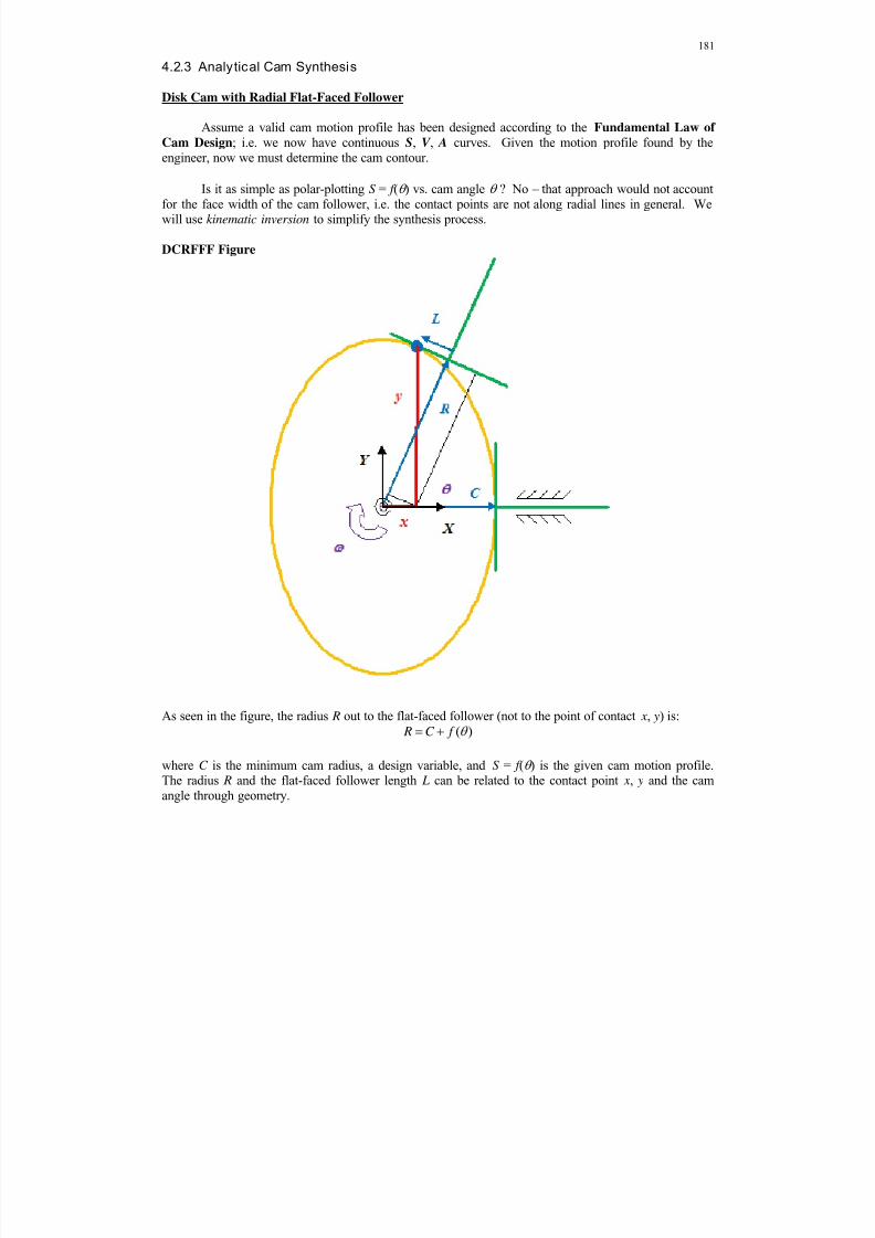
8/11/2019 Mechanism kinematics & dynamics.pdf
http://slidepdf.com/reader/full/mechanism-kinematics-dynamicspdf 181/269
181
4.2.3 Analytical Cam Synthesis
Disk Cam with Radial Flat-Faced Follower
Assume a valid cam motion profile has been designed according to the Fundamental Law of
Cam Design; i.e. we now have continuous S, V , A curves. Given the motion profile found by theengineer, now we must determine the cam contour.
Is it as simple as polar-plotting S = f ( ) vs. cam angle ? No – that approach would not accountfor the face width of the cam follower, i.e. the contact points are not along radial lines in general. Wewill use kinematic inversion to simplify the synthesis process.
DCRFFF Figure
As seen in the figure, the radius R out to the flat-faced follower (not to the point of contact x, y) is:( ) R C f
where C is the minimum cam radius, a design variable, and S = f ( ) is the given cam motion profile.The radius R and the flat-faced follower length L can be related to the contact point x, y and the camangle through geometry.
8/11/2019 Mechanism kinematics & dynamics.pdf
http://slidepdf.com/reader/full/mechanism-kinematics-dynamicspdf 182/269
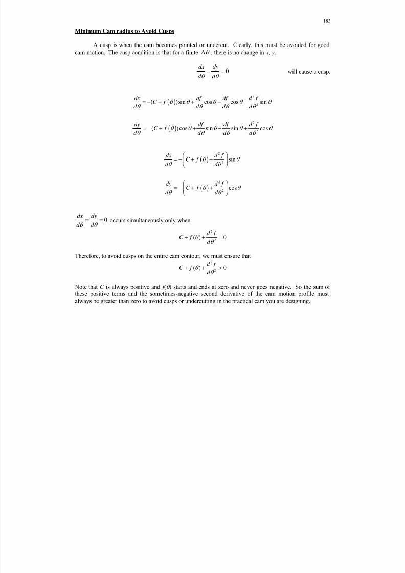
8/11/2019 Mechanism kinematics & dynamics.pdf
http://slidepdf.com/reader/full/mechanism-kinematics-dynamicspdf 183/269
183
Minimum Cam radius to Avoid Cusps
A cusp is when the cam becomes pointed or undercut. Clearly, this must be avoided for good
cam motion. The cusp condition is that for a finite , there is no change in x, y.
0dx dy
d d
will cause a cusp.
2
2
2
2
( )sin cos cos sin
( )cos sin sin cos
dx df df d f C f
d d d d
dy df df d f C f
d d d d
2
2
2
2
sin
cos
dx d f C f d d
dy d f C f
d d
0dx dy
d d occurs simultaneously only when
2
2( ) 0d f C f
d
Therefore, to avoid cusps on the entire cam contour, we must ensure that2
2( ) 0
d f C f
d
Note that C is always positive and f ( ) starts and ends at zero and never goes negative. So the sum ofthese positive terms and the sometimes-negative second derivative of the cam motion profile mustalways be greater than zero to avoid cusps or undercutting in the practical cam you are designing.

8/11/2019 Mechanism kinematics & dynamics.pdf
http://slidepdf.com/reader/full/mechanism-kinematics-dynamicspdf 184/269
184
Disk Cam with Radial Flat-Faced Follower Design Example
Specify a full-cycloidal rise with a total lift of 50 mm, followed by a high dwell, a symmetricfull-cycloidal return with a total fall of 50 mm, and then a low dwell. Each of these four motion steps
occurs for 90 of cam shaft rotation.
The full-cycloidal rise and fall cam motion profile associated with this specification is shown below. Clearly, this satisfies the Fundamental Law of Cam Design because the position, velocity, andacceleration curves are continuous. The jerk is not continuous, but it remains finite over all cam angles.
0 50 100 150 200 250 300 3500
10
20
30
40
50
S
0 50 100 150 200 250 300 350
-50
0
50
V
0 50 100 150 200 250 300 350
-100
-50
0
50
100
A
0 50 100 150 200 250 300 350-500
0
500
J
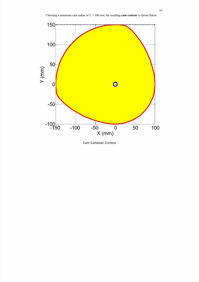
8/11/2019 Mechanism kinematics & dynamics.pdf
http://slidepdf.com/reader/full/mechanism-kinematics-dynamicspdf 185/269
185
Choosing a minimum cam radius of C = 100 mm, the resulting cam contour is shown below.
Cam Cartesian Contour
-150 -100 -50 0 50 100-100
-50
0
50
100
150
X (mm)
Y ( m
m )
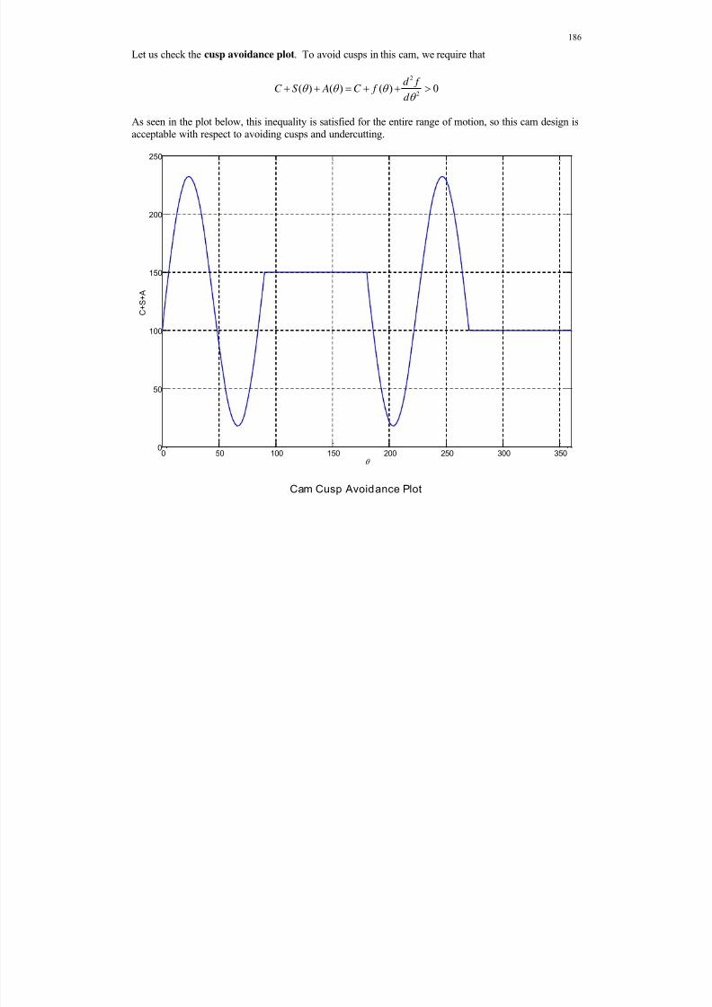
8/11/2019 Mechanism kinematics & dynamics.pdf
http://slidepdf.com/reader/full/mechanism-kinematics-dynamicspdf 186/269
186
Let us check the cusp avoidance plot. To avoid cusps in this cam, we require that
2
2( ) ( ) ( ) 0
d f C S A C f
d
As seen in the plot below, this inequality is satisfied for the entire range of motion, so this cam design is
acceptable with respect to avoiding cusps and undercutting.
Cam Cusp Avoidance Plot
0 50 100 150 200 250 300 3500
50
100
150
200
250
C + S + A

8/11/2019 Mechanism kinematics & dynamics.pdf
http://slidepdf.com/reader/full/mechanism-kinematics-dynamicspdf 187/269
187
Cam/Follower Animation Snapshot for2 60 (CW)
-200 -150 -100 -50 0 50 100 150 200-200
-150
-100
-50
0
50
100
150
200
X (m)
Y ( m )
8/11/2019 Mechanism kinematics & dynamics.pdf
http://slidepdf.com/reader/full/mechanism-kinematics-dynamicspdf 188/269
8/11/2019 Mechanism kinematics & dynamics.pdf
http://slidepdf.com/reader/full/mechanism-kinematics-dynamicspdf 189/269
189
damping A linear model for energy loss due to friction and other energy dissipaters,for either translational or rotational motion. Damping is provided by avirtual viscous dashpot (an automotive shock system is a real example).
amplitude The maximum magnitude of a sinusoidal oscillation.
phase angle Angle in a single sinusoidal function that indicates the amount of lead orlag of a cosine or sine wave relative to the standard cosine or sine wave.
differential equation An equation in which the unknown appears with its time derivatives.
initial conditions Given values at time t = 0 for the output and its time derivatives. Theremust be as many initial conditions as the order of the differential equation.
input The external forcing function that drives a dynamic system.
output The variable of interest in motion of a dynamic system.
free vibrations Vibrations in the absence of a forcing function.
homogeneous solution Transient solution due to initial conditions and the external input forcingfunction, yielding zero in the ODE.
transient vibrations Vibrations that disappear given enough time.
forced vibrations Vibrations due to an external input forcing function.
particular solution Steady-state solution due to the external input forcing function. There isalso a transient solution due to the external input forcing function.
steady-state vibrations Vibrations that do not disappear as time increases.
forcing function The input actuation provided by an external source.
driving frequency The rate at which an external input forces a vibratory system, either
cyclical f , or circular .
damped frequency The rate at which an unforced, damped vibratory system tends to vibrate,
either cyclical f d , or circular d .
logarithmic decrement The natural logarithm of the ratio of two consecutive points, separated bythe damped time period T d , on a unforced underdamped vibratory wave.
beat frequency Vibrational phenomenon wherein two frequencies in a dynamic system areclose in value, causing a vibration within a vibrational envelope.
resonance This condition occurs when the driving frequency is the same as, or
close to, the system’s natural frequency n. In this case the resultingamplitude of the steady-state vibration becomes very large.

8/11/2019 Mechanism kinematics & dynamics.pdf
http://slidepdf.com/reader/full/mechanism-kinematics-dynamicspdf 190/269
190
frequency response The plots of system amplitude and phase angle vs. independent variableinput frequency.
critical shaft speed The angular shaft velocity that excites the natural frequency of a rotatingdynamic system. When driven at the critical speed, resonance occurs, acondition generally to be avoided at all costs.
transmissibility The ratio of the maximum force transmitted to the base over the maximuminput force magnitude in a vibratory dynamic system.
vibration mode Characteristic shape at which a dynamic system will vibrate. Multi-dofsystems have multiple modes that sum to yield the total time response.
A linear system is one in which all governing equations (differential, algebraic) are linear.Linear systems satisfy the principles of linear superposition and homogeneity. Let u(t ) be the input
and y(t ) be the output. Further, ( ) ( )u t y t indicates a system yielding output y(t ) given input u(t ).
1) linear superposition
if 1 1( ) ( )u t y t and 2 2( ) ( )u t y t then 1 2 1 2( ) ( ) ( ) ( )u t u t y t y t
2) homogeneity
if ( ) ( )u t y t then ( ) ( )u t y t
where is any constant.

8/11/2019 Mechanism kinematics & dynamics.pdf
http://slidepdf.com/reader/full/mechanism-kinematics-dynamicspdf 191/269
191
6. Vibrational Systems Modeling
6.1 Zeroth-Order Systems
Calculation of Spring Constants
Helical Coiled Spring. The jagged springs indicated so far represent physical translationalsprings coiled from an elastic wire into a helical shape about a central axis. For this physical spring,from Strength of Materials, the linear spring constant k for small displacements is given below.
4
38
Gd k
nD
whereG material shear modulus N/m2
d wire diameter mn number of spring coils unitless D diameter of spring coiling m
This type of coiled physical spring is common; however, there are many mechanical systemswithout a clear spring such as above. Instead, their elastic properties are provided by distributedmaterial in the system. Here we present several such distributed springs that are modeled as linearsprings for small displacements, as follows.
For the following 4 translational springs, the following method is used. For each given physical
situation, we find the displacement under an applied force F , from Strength of Materials. Then the
spring stiffness constant k is found from Hooke’s Law F = k : k = F / . Below we assume that the forceis applied and the displacement measured at the end of the cantilevered beam and in the center of theother beams.
f(t)
d
D f(t)
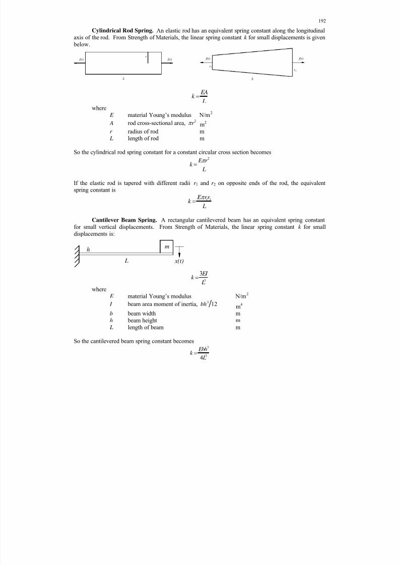
8/11/2019 Mechanism kinematics & dynamics.pdf
http://slidepdf.com/reader/full/mechanism-kinematics-dynamicspdf 192/269
192
Cylindrical Rod Spring. An elastic rod has an equivalent spring constant along the longitudinalaxis of the rod. From Strength of Materials, the linear spring constant k for small displacements is given below.
EAk
L
where E material Young’s modulus N/m
2
A rod cross-sectional area, 2r m2
r radius of rod m L length of rod m
So the cylindrical rod spring constant for a constant circular cross section becomes2
E r k
L
If the elastic rod is tapered with different radii r 1 and r 2 on opposite ends of the rod, the equivalentspring constant is
1 2 E rr k
L
Cantilever Beam Spring. A rectangular cantilevered beam has an equivalent spring constant
for small vertical displacements. From Strength of Materials, the linear spring constant k for smalldisplacements is:
3
3 EI k
L
where E material Young’s modulus N/m2
I beam area moment of inertia,3
12bh m4
b beam width mh beam height m L length of beam m
So the cantilevered beam spring constant becomes3
34
Ebhk
L
f(t)r
L
f(t) f(t)
r
L
f(t)
1
r 2
m
L x(t)
h
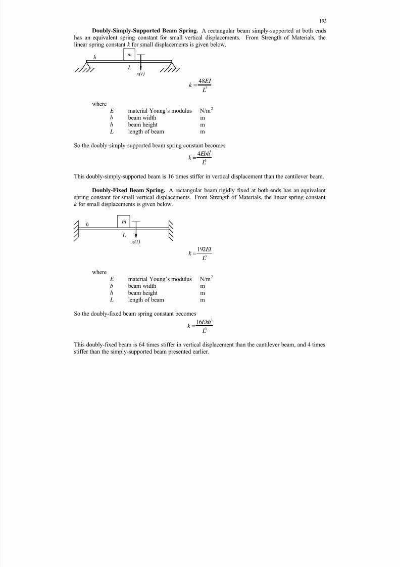
8/11/2019 Mechanism kinematics & dynamics.pdf
http://slidepdf.com/reader/full/mechanism-kinematics-dynamicspdf 193/269
193
Doubly-Simply-Supported Beam Spring. A rectangular beam simply-supported at both endshas an equivalent spring constant for small vertical displacements. From Strength of Materials, thelinear spring constant k for small displacements is given below.
3
48 EI k
L
where E material Young’s modulus N/m2
b beam width mh beam height m L length of beam m
So the doubly-simply-supported beam spring constant becomes
3
34 Ebhk
L
This doubly-simply-supported beam is 16 times stiffer in vertical displacement than the cantilever beam.
Doubly-Fixed Beam Spring. A rectangular beam rigidly fixed at both ends has an equivalentspring constant for small vertical displacements. From Strength of Materials, the linear spring constantk for small displacements is given below.
3
192 EI k
L
where E material Young’s modulus N/m
2
b beam width mh beam height m L length of beam m
So the doubly-fixed beam spring constant becomes3
3
16 Ebhk
L
This doubly-fixed beam is 64 times stiffer in vertical displacement than the cantilever beam, and 4 timesstiffer than the simply-supported beam presented earlier.
m
L x(t)
h
m
L x(t)
h

8/11/2019 Mechanism kinematics & dynamics.pdf
http://slidepdf.com/reader/full/mechanism-kinematics-dynamicspdf 194/269
194
Air Spring. An enclosed volume of air has an equivalent spring constant for smalldisplacements. From Fluid Mechanics for compressible air, the linear spring constant k for smalldisplacements is given below.
2PA
k V
where
ratio of specific heats unitlessP enclosed air pressure N/m2
A enclosed air cross-sectional area m2
V enclosed air volume m3
These six spring constant examples are all for translational springs, so their spring constant k units should all be N/m. The material Young’s Modulus E and Shear Modulus G for steel are:
9 2200 GPa = 200 10 N / m E 9 279 GPa = 79 10 N / mG
Let us now check the units for the previous six spring constants.
4 4
3 2 3
Nm N
8 m m m
Gd
nD
2
2
Nm N
m m m
EA
L
4
3 2 3
3 Nm N
m m m
EI
L
3 3
3 2 3
4 N(m)m N
m m m
Ebh
L
3 3
3 2 3
16 N(m)m N
m m m
Ebh
L
2 4
2 3
Nm N
m m m
PA
V
All units are correct for a translational spring, i.e. N/m.
We have also used torsional springs in our mechanical systems models. Torsional springs can beconstructed of a coiled elastic material, spiraling in one plane. An elastic cylindrical rod also provides atorsional spring effect when torque about the longitudinal axis of the rod. Additionally, a fixed-simply-supported beam also provides a torsional spring effect.
f(t)

8/11/2019 Mechanism kinematics & dynamics.pdf
http://slidepdf.com/reader/full/mechanism-kinematics-dynamicspdf 195/269
195
Torsional Rod Spring. An elastic rod has an equivalent spring constant about the longitudinalaxis of the rod. From Strength of Materials, the torsional spring constant k R for small angulardisplacements is given below.
4
2 R
G r k
L
whereG material shear modulus N/m
2
r radius of rod m L length of rod m
If the torsional shaft is hollow, the torsional spring stiffness constant is
4 4( )
2
o i R
G r r k
L
where r o and r i are the outer and inner shaft radii, respectively.
Fixed-Simply-Supported Torsional Beam Spring. A rectangular beam rigidly fixed at one endand simply supported on the other has an equivalent torsional spring constant for small angulardisplacements. From Strength of Materials, the torsional spring constant k R for small displacements is
given below.
4 R
EI k
L
where
E material Young’s modulus N/m2
b beam width mh beam height or thickness m L length of beam m
So the fixed-simply-supported torsional beam spring constant becomes3
3 R
Ebhk
L
r
L
(t) (t)
m
L
(t)h
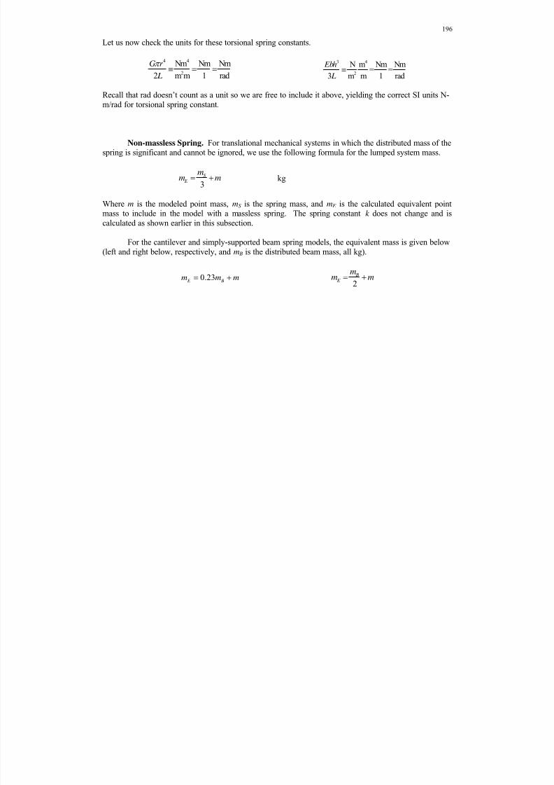
8/11/2019 Mechanism kinematics & dynamics.pdf
http://slidepdf.com/reader/full/mechanism-kinematics-dynamicspdf 196/269

8/11/2019 Mechanism kinematics & dynamics.pdf
http://slidepdf.com/reader/full/mechanism-kinematics-dynamicspdf 197/269
197
Calculation of Damping Constants
In general the damping coefficient for a physical system is harder to identify and calculate thanthe mass and spring constants. This subsection presents 4 equivalent damping coefficient cases. Many physical systems have no identifiable damping dashpot, but a viscous damping coefficient c is includedto account for friction losses in the system, using a simple linear model (the law for linear dashpotswhere the friction force is proportional to the velocity).
Also see the later section on logarithmic decrement, where the damping coefficient c can beestimated from experimental observations.
Dashpot. The piston-based dampers indicated so far represent physical dashpots with a pistonmoving (translating in a reciprocating fashion) in a viscous fluid to remove energy from the system,such as in an automotive shock absorber. For this physical dashpot, from Fluid Mechanics, the linearviscous damping coefficient c for small velocities is given below.
3
3
61
r h wc
w r
where
fluid viscosity N-s/m2
r piston radius mh piston height mw wall thickness r o – r m
f(t)
h
r
w

8/11/2019 Mechanism kinematics & dynamics.pdf
http://slidepdf.com/reader/full/mechanism-kinematics-dynamicspdf 198/269

8/11/2019 Mechanism kinematics & dynamics.pdf
http://slidepdf.com/reader/full/mechanism-kinematics-dynamicspdf 199/269
199
Rotational dashpot. We have also used torsional dashpots in our mechanical systems models.Torsional dashpots can be constructed in a similar manner to a translational dashpot, but thereciprocating motion is rotary about the center axis, instead of translational. From Fluid Mechanics, thelinear rotational viscous damping coefficient c R for small angular velocities is given below.
3
0
28
R
h r c r
w h
where
fluid viscosity N-s/m2 r piston radius mh piston height mw wall thickness r o – r m
h0 height from base to rotating piston m
(t)
h
r
w
h 0

8/11/2019 Mechanism kinematics & dynamics.pdf
http://slidepdf.com/reader/full/mechanism-kinematics-dynamicspdf 200/269
200
Journal bearing. A journal bearing also has a fluid providing rotational damping. From FluidMechanics, the linear rotational viscous damping coefficient c R for small angular velocities is given below.
32 R
wr c
where
fluid viscosity N-s/m2 w base thickness mr bearing radius m
journal bearing fluid clearance m
Let us now check the units for these torsional damping coefficients.
3 3
2
0
Ns m Nms2 m Nms
8 m m rad
h r r
w h
3 4
2
2 Ns m Nms Nms
m m rad
wr
Recall that rad doesn’t count as a unit so we are free to include it above, yielding the correct SI units N-m-s/rad for torsional damping coefficient.
r
w
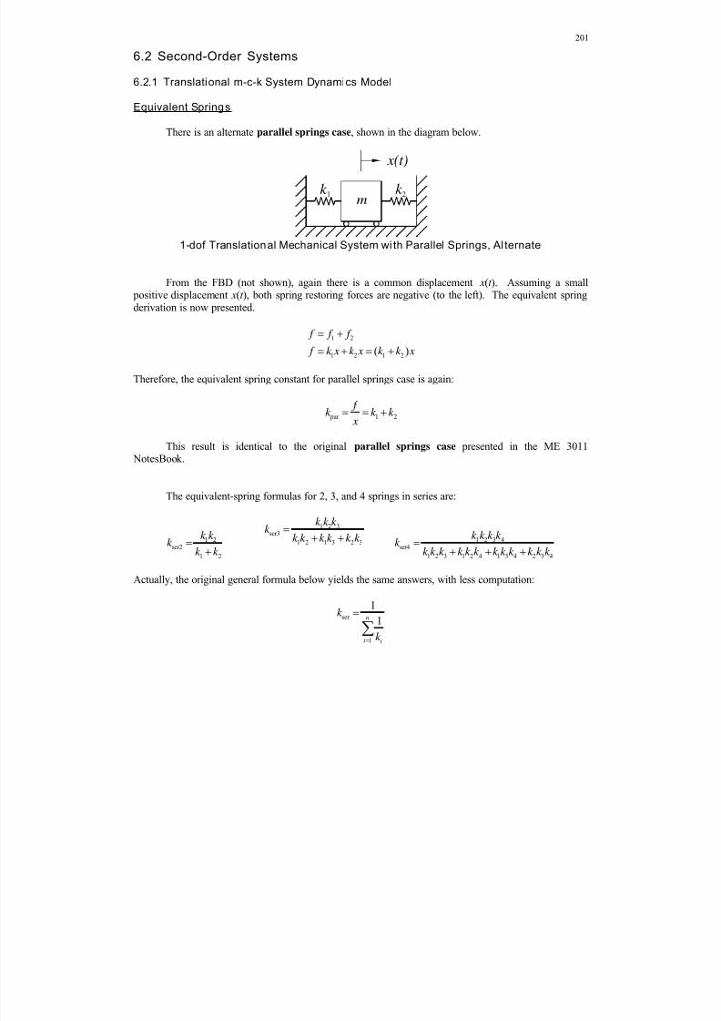
8/11/2019 Mechanism kinematics & dynamics.pdf
http://slidepdf.com/reader/full/mechanism-kinematics-dynamicspdf 201/269
201
6.2 Second-Order Systems
6.2.1 Translational m-c-k System Dynamics Model
Equivalent Springs
There is an alternate parallel springs case, shown in the diagram below.
1-dof Translational Mechanical System wi th Parallel Springs, Al ternate
From the FBD (not shown), again there is a common displacement x(t ). Assuming a small positive displacement x(t ), both spring restoring forces are negative (to the left). The equivalent springderivation is now presented.
1 2
1 2 1 2( )
f f f
f k x k x k k x
Therefore, the equivalent spring constant for parallel springs case is again:
par 1 2
f
k k k x
This result is identical to the original parallel springs case presented in the ME 3011 NotesBook.
The equivalent-spring formulas for 2, 3, and 4 springs in series are:
1 2ser2
1 2
k k k
k k
1 2 3ser3
1 2 1 3 2 3
k k k k
k k k k k k
1 2 3 4ser4
1 2 3 1 2 4 1 3 4 2 3 4
k k k k k
k k k k k k k k k k k k
Actually, the original general formula below yields the same answers, with less computation:
ser
1
1
1n
i i
k
k
x(t)
mk k 1 2
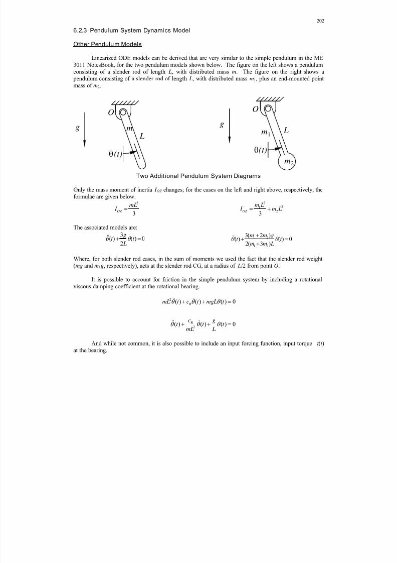
8/11/2019 Mechanism kinematics & dynamics.pdf
http://slidepdf.com/reader/full/mechanism-kinematics-dynamicspdf 202/269
202
6.2.3 Pendulum System Dynamics Model
Other Pendulum Models
Linearized ODE models can be derived that are very similar to the simple pendulum in the ME3011 NotesBook, for the two pendulum models shown below. The figure on the left shows a pendulumconsisting of a slender rod of length L, with distributed mass m. The figure on the right shows a pendulum consisting of a slender rod of length L, with distributed mass m1, plus an end-mounted pointmass of m2.
Two Addit ional Pendulum System Diagrams
Only the mass moment of inertia I OZ changes; for the cases on the left and right above, respectively, theformulae are given below.
2
3OZ
mL I
221
23
OZ
m L I m L
The associated models are:3
( ) ( ) 02
gt t
L
1 2
1 2
3( 2 )( ) ( ) 0
2( 3 )
m m gt t
m m L
Where, for both slender rod cases, in the sum of moments we used the fact that the slender rod weight(mg and m1g, respectively), acts at the slender rod CG, at a radius of L/2 from point O.
It is possible to account for friction in the simple pendulum system by including a rotationalviscous damping coefficient at the rotational bearing.
2
2
( ) ( ) ( ) 0
( ) ( ) ( ) 0
R
R
mL t c t mgL t
c gt t t
mL L
And while not common, it is also possible to include an input forcing function, input torque (t )at the bearing.
g m L
O
(t)2
1
gm
m(t)
O
L

8/11/2019 Mechanism kinematics & dynamics.pdf
http://slidepdf.com/reader/full/mechanism-kinematics-dynamicspdf 203/269
203
2 2
1( ) ( ) ( ) ( ) R
c gt t t t
mL L mL
Finally, if we model a horizontal pendulum, the restoring torque of gravity disappears and wehave the dynamic model of a gravity-neutral single rotating link.
2 21( ) ( ) ( ) Rct t t
mL mL

8/11/2019 Mechanism kinematics & dynamics.pdf
http://slidepdf.com/reader/full/mechanism-kinematics-dynamicspdf 204/269
204
6.2.4 Uniform Circular MotionUniform circular motion (UCM), wherein a point P at the end of a fixed-length link of length r
rotating in the XY plane about a fixed point O with a constant angular velocity (see figure below)generates Simple Harmonic Motion, like an unforced, undamped m-k translational mechanical system.
Uniform Circular Motion Diagram
In this UCM case no differential equations or solutions are required. Simultaneously simpleharmonic motion (SHM) is generated in the X with a pure cosine wave (with no phase angle) and in theY with a pure sine wave (with no phase angle); see the figure below, generated by UCM.m . Since
angular velocity is constant, the angle linearly increases with time, ( )t t . With 0 = 0 at t = 0, this
system will generate SHM in the X and Y directions indefinitely, repeating every 360 deg or 2 rad.
( ) cos ( ) cos
( ) sin ( ) sin
x t r t r t
y t r t r t
MATLAB UCM Animation
r
(t)
P
O X
Y

8/11/2019 Mechanism kinematics & dynamics.pdf
http://slidepdf.com/reader/full/mechanism-kinematics-dynamicspdf 205/269
205
6.4 Additional 1-dof Vibrational Systems Models
1-dof Vibrational Systems
Derive the vibrational equation of motion for each given mechanical system below.
1. m-c-k translational systems with parallel and series springs and dampers
The ME 3011 NotesBook presented the derivation of equivalent translational springs for the parallel springs and series springs cases. Translational dashpots also follow the same formulas for theirrespective parallel and series cases.
Considering the parallel-case figure shown below,
1-dof Translational Mechanical System with Parallel Springs and Dashpots
the system model is:
1 2 1 2( ) ( ) ( ) ( ) ( ) ( )mx t c c x t k k x t f t
Considering the series-case figure shown below,
1-dof Translational Mechanical System with Series Springs and Dashpots
the system model is:
1 2 1 2
1 2 1 2
( ) ( ) ( ) ( )c c k k
mx t x t x t f t c c k k
x(t)
m
k k 1 2
c
c1
2
f(t)
x(t)
m
k k 1 2
c1 f(t)c2

8/11/2019 Mechanism kinematics & dynamics.pdf
http://slidepdf.com/reader/full/mechanism-kinematics-dynamicspdf 206/269
206
2. J-cR-kR rotational systems with parallel and series springs and dampers
The same type of second-order models result for the rotational systems as in the translationalsystems presented on the last page, with regard to parallel and series arrangements of rotational springsand dashpots.
Considering the parallel case, the system model is given below.
1 2 1 2( ) ( ) ( ) ( ) ( ) ( ) R R R R J t c c t k k t t
Considering the series case, the system model is given below.
1 2 1 2
1 2 1 2
( ) ( ) ( ) ( ) R R R R
R R R R
c c k k J t t t t
c c k k

8/11/2019 Mechanism kinematics & dynamics.pdf
http://slidepdf.com/reader/full/mechanism-kinematics-dynamicspdf 207/269
207
Compound m-c-k translational systems wi th parallel and series springs and dampers
Certain real-world systems may require more complicated models with combinations of springsand dampers in parallel and in series. There are infinite possible combinations of such models, dictated by the real-world component arrangement. The next two sections present two such possibilities.
3. Parallel springs and dampers in series
The figure below shows two sets of parallel springs arranged in series. For clarity, the dashpotsare not shown but they have the same arrangement.
The second figure shows a simplified diagram for this case.
Using the parallel- and then serial-springs equivalent spring formulas derived in the ME 3011 NotesBook:
1 3
2 4
a
b
k k k
k k k
1 2 2 3 1 4 3 4
1 2 3 4
a beq
a b
k k k k k k k k k k k
k k k k k k
The system model is now given.
( ) ( ) ( ) ( )eq eq
mx t c x t k x t f t
where 1 2 2 3 1 4 3 4
1 2 3 4
eq
c c c c c c c cc
c c c c
This example is for a translational system, but equivalent results exist for an analogous rotationalsystem.
1
3
k x(t)
mk
2
4
k
k f(t)
k
x(t)
mk
f(t)a b
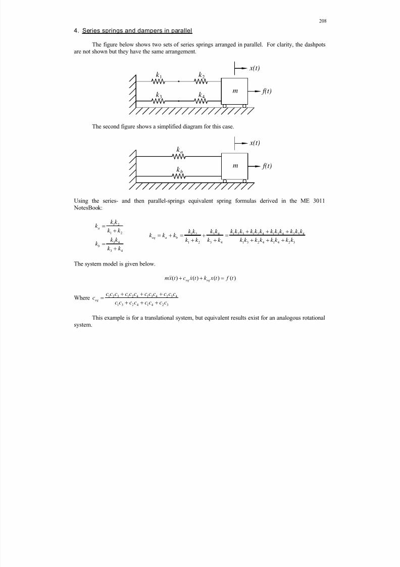
8/11/2019 Mechanism kinematics & dynamics.pdf
http://slidepdf.com/reader/full/mechanism-kinematics-dynamicspdf 208/269
208
4. Series springs and dampers in parallel
The figure below shows two sets of series springs arranged in parallel. For clarity, the dashpotsare not shown but they have the same arrangement.
The second figure shows a simplified diagram for this case.
Using the series- and then parallel-springs equivalent spring formulas derived in the ME 3011 NotesBook:
1 2
1 2
3 4
3 4
a
b
k k k
k k
k k k
k k
3 4 1 2 3 1 2 4 1 3 4 2 3 41 2
1 2 3 4 1 3 2 4 1 4 2 3
eq a b
k k k k k k k k k k k k k k k k k k k
k k k k k k k k k k k k
The system model is given below.
( ) ( ) ( ) ( )eq eqmx t c x t k x t f t
Where 1 2 3 1 2 4 1 3 4 2 3 4
1 3 2 4 1 4 2 3
eq
c c c c c c c c c c c cc
c c c c c c c c
This example is for a translational system, but equivalent results exist for an analogous rotationalsystem.
1
3
k
x(t)
mk
2
4
k
k f(t)
k x(t)
mk
f(t)
a
b
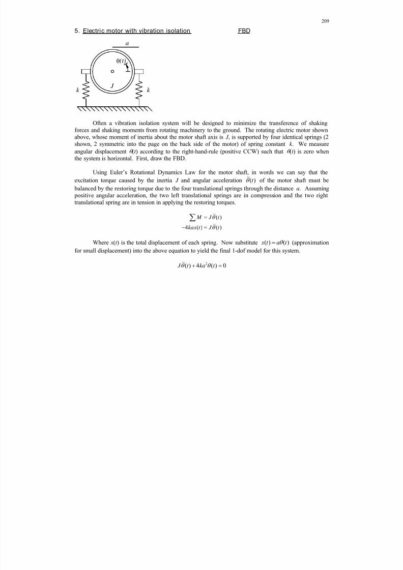
8/11/2019 Mechanism kinematics & dynamics.pdf
http://slidepdf.com/reader/full/mechanism-kinematics-dynamicspdf 209/269
209
5. Electric motor with vibration isolation FBD
Often a vibration isolation system will be designed to minimize the transference of shakingforces and shaking moments from rotating machinery to the ground. The rotating electric motor shownabove, whose moment of inertia about the motor shaft axis is J , is supported by four identical springs (2shown, 2 symmetric into the page on the back side of the motor) of spring constant k . We measure
angular displacement (t ) according to the right-hand-rule (positive CCW) such that (t ) is zero whenthe system is horizontal. First, draw the FBD.
Using Euler’s Rotational Dynamics Law for the motor shaft, in words we can say that the
excitation torque caused by the inertia J and angular acceleration ( )t of the motor shaft must be
balanced by the restoring torque due to the four translational springs through the distance a. Assuming positive angular acceleration, the two left translational springs are in compression and the two righttranslational spring are in tension in applying the restoring torques.
( )
4 ( ) ( )
M J t
kax t J t
Where x(t ) is the total displacement of each spring. Now substitute ( ) ( ) x t a t (approximation
for small displacement) into the above equation to yield the final 1-dof model for this system.
2( ) 4 ( ) 0 J t ka t
J k
a
(t)
k

8/11/2019 Mechanism kinematics & dynamics.pdf
http://slidepdf.com/reader/full/mechanism-kinematics-dynamicspdf 210/269
210
6. Sprung mass/cylinder FBDs
In this dynamic system, m1 is the point mass suspended by cable about a cylindrical pulley ofmass m2 and radius r . The other end of the cable is attached to a linear translational spring withconstant k . We measure displacement x(t ) (positive downward) from the neutral position of the spring.
We also measure angular displacement (t ) with the right-hand-rule (positive CCW) such that it is zerowhen x(t ) is zero. First, draw the FBDs.
Using Newton’s Second Law for the point mass:
1 1 ( ) X
F m g T m x t
Using Euler’s Rotational Dynamics Law for the cylinder:
( ( )) ( ) Z
M Tr kr x t J t
Where ( ) x t is the total displacement of the spring ( is the static deflection of the spring due
to gravity). Also, the mass moment of inertia of the cylindrical pulley is
2
2 2 J m r . Now substitute( ) ( ) x t r t and ( ) ( ) x t r t into the above equations.
1 1
2
2
( )
( ( )) ( )2
m g T m r t
m r Tr kr r t t
We can combine the above two equations to eliminate the cable tension T .
1 1
22 2
1 1
( )
( ) ( ( )) ( )2
T m g m r t
m r m gr m r t kr r t t
At static equilibrium we have 1m gr kr , so the final 1-dof model for this system is
22 2 2
1
21
( ) ( ) ( )2
( ) ( ) 02
m r m r t kr t t
mm t k t
m
m
k
x(t)
r (t)
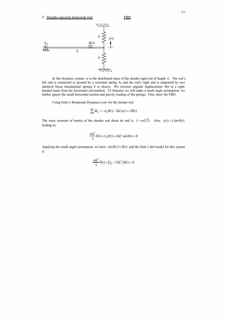
8/11/2019 Mechanism kinematics & dynamics.pdf
http://slidepdf.com/reader/full/mechanism-kinematics-dynamicspdf 211/269
211
7. Doubly-sprung torsional rod FBD
In this dynamic system, m is the distributed mass of the slender rigid rod of length L. The rod’sleft end is connected to ground by a torsional spring k R and the rod’s right end is supported by two
identical linear translational springs k as shown. We measure angular displacement (t ) in a right-handed sense from the horizontal rod position. To linearize we will make a small angle assumption; wefurther ignore the small horizontal motion and gravity loading of the springs. First, draw the FBD.
Using Euler’s Rotational Dynamics Law for the slender rod:
( ) 2 ( ) ( ) Z R M k t kLy t J t
The mass moment of inertia of the slender rod about its end is 2 3 J mL . Also, ( ) sin ( ) y t L t ,
leading to:
22( ) ( ) 2 sin ( ) 0
3 R
mLt k t kL t
Applying the small angle assumption, we have sin ( ) ( )t t and the final 1-dof model for this system
is
2
2( ) 2 ( ) 03
R
mLt k kL t
L
k
y(t)
(t)
k
k R

8/11/2019 Mechanism kinematics & dynamics.pdf
http://slidepdf.com/reader/full/mechanism-kinematics-dynamicspdf 212/269
212
8. Sprung roll ing cylinder FBD
In this dynamic system, a cylinder of mass m and radius r rolls without slipping on a horizontalsurface. The cylinder center is attached to the ground via a linear translational spring with constant k .We measure displacement x(t ) (positive to the right) from the neutral position of the spring. We also
measure angular displacement (t ) with the right-hand-rule (positive CCW) such that it is zero when x(t )is zero. First, draw the FBD.
Using Newton’s Second Law for the cylinder (F f is the force due to friction):
( ) ( ) X f F F kx t mx t
Using Euler’s Rotational Dynamics Law for the cylinder:
( ) Z f M F r J t
We can combine the above two equations to eliminate the friction force F f :
( ) ( )
( ( ) ( )) ( )
f F mx t kx t
mx t kx t r J t
The mass moment of inertia of the cylindrical pulley is 2 2 J mr . Now substitute
( ) ( )t x t r into the above equation to express the motion in terms of x(t ).
2
( )( ( ) ( ))2
mr x t mx t kx t r r
The final 1-dof model for this system is
3( ) ( ) 0
2mx t kx t
m
k
x(t)
r (t)
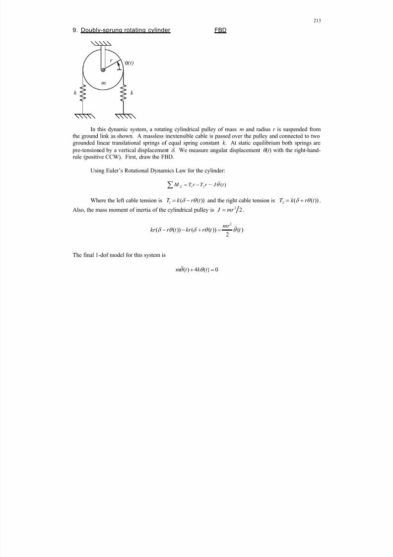
8/11/2019 Mechanism kinematics & dynamics.pdf
http://slidepdf.com/reader/full/mechanism-kinematics-dynamicspdf 213/269
213
9. Doubly-sprung rotating cylinder FBD
In this dynamic system, a rotating cylindrical pulley of mass m and radius r is suspended fromthe ground link as shown. A massless inextensible cable is passed over the pulley and connected to twogrounded linear translational springs of equal spring constant k . At static equilibrium both springs are
pre-tensioned by a vertical displacement . We measure angular displacement (t ) with the right-hand-rule (positive CCW). First, draw the FBD.
Using Euler’s Rotational Dynamics Law for the cylinder:
1 2 ( ) Z
M T r T r J t
Where the left cable tension is 1 ( ( ))T k r t and the right cable tension is 2 ( ( ))T k r t .
Also, the mass moment of inertia of the cylindrical pulley is 2 2 J mr .
2
( ( )) ( ( )) ( )2
mr kr r t kr r t t
The final 1-dof model for this system is
( ) 4 ( ) 0m t k t
m
k
r (t)
k
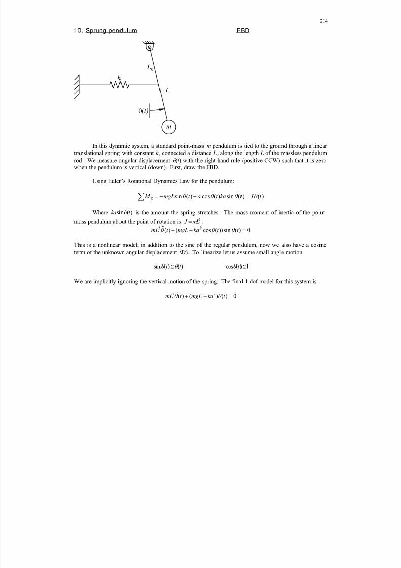
8/11/2019 Mechanism kinematics & dynamics.pdf
http://slidepdf.com/reader/full/mechanism-kinematics-dynamicspdf 214/269
214
10. Sprung pendulum FBD
In this dynamic system, a standard point-mass m pendulum is tied to the ground through a linear
translational spring with constant k , connected a distance L0 along the length L of the massless pendulumrod. We measure angular displacement (t ) with the right-hand-rule (positive CCW) such that it is zerowhen the pendulum is vertical (down). First, draw the FBD.
Using Euler’s Rotational Dynamics Law for the pendulum:
sin ( ) cos ( ) sin ( ) ( ) Z M mgL t a t ka t J t
Where sin ( )ka t is the amount the spring stretches. The mass moment of inertia of the point-
mass pendulum about the point of rotation is 2 J mL .
2 2
( ) ( cos ( ))sin ( ) 0mL t mgL ka t t
This is a nonlinear model; in addition to the sine of the regular pendulum, now we also have a cosine
term of the unknown angular displacement (t ). To linearize let us assume small angle motion.
sin ( ) ( )t t
cos ( ) 1t
We are implicitly ignoring the vertical motion of the spring. The final 1-dof model for this system is
2 2( ) ( ) ( ) 0mL t mgL ka t
m
k
L
(t)
L0
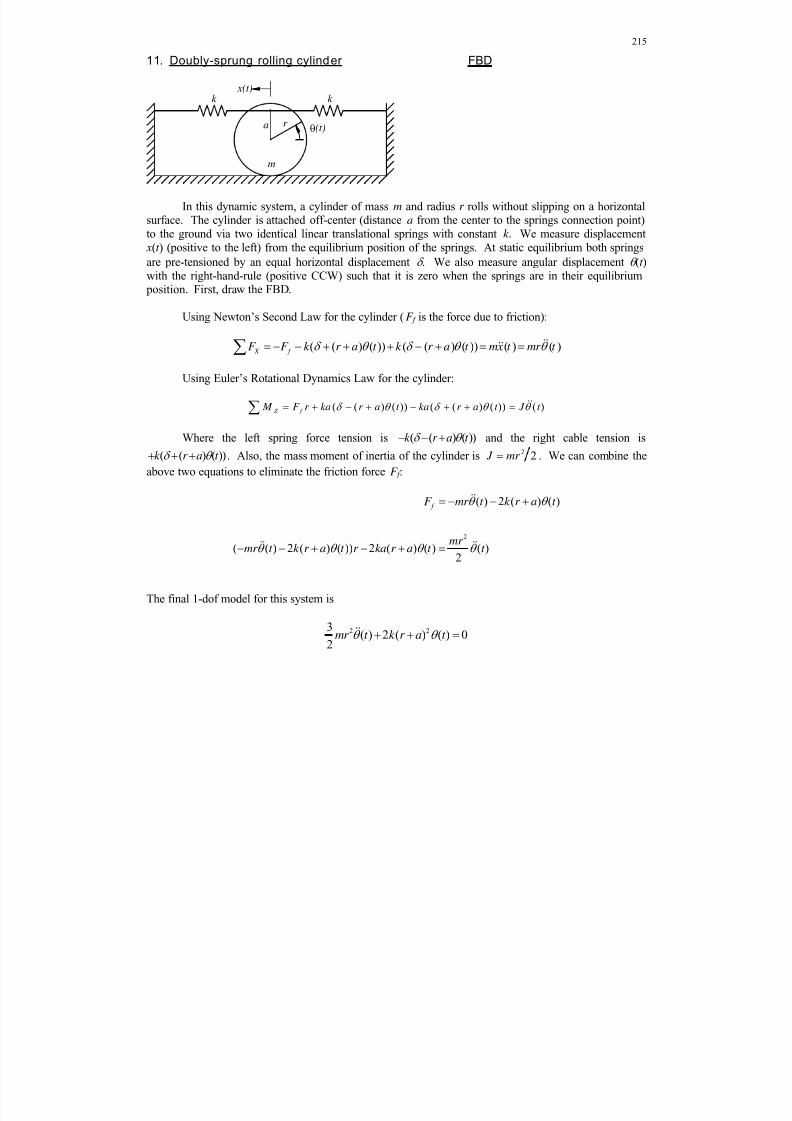
8/11/2019 Mechanism kinematics & dynamics.pdf
http://slidepdf.com/reader/full/mechanism-kinematics-dynamicspdf 215/269
215
11. Doubly-sprung rolling cylinder FBD
In this dynamic system, a cylinder of mass m and radius r rolls without slipping on a horizontalsurface. The cylinder is attached off-center (distance a from the center to the springs connection point)to the ground via two identical linear translational springs with constant k . We measure displacement x(t ) (positive to the left) from the equilibrium position of the springs. At static equilibrium both springs
are pre-tensioned by an equal horizontal displacement . We also measure angular displacement (t )with the right-hand-rule (positive CCW) such that it is zero when the springs are in their equilibrium position. First, draw the FBD.
Using Newton’s Second Law for the cylinder (F f is the force due to friction):
( ( ) ( )) ( ( ) ( )) ( ) ( ) X f F F k r a t k r a t mx t mr t
Using Euler’s Rotational Dynamics Law for the cylinder:
( ( ) ( )) ( ( ) ( )) ( ) Z f
M F r ka r a t ka r a t J t
Where the left spring force tension is ( ( ) ( ))k r a t and the right cable tension is
( ( ) ( ))k r a t . Also, the mass moment of inertia of the cylinder is 2 2 J mr . We can combine theabove two equations to eliminate the friction force F f :
2
( ) 2 ( ) ( )
( ( ) 2 ( ) ( )) 2 ( ) ( ) ( )2
f F mr t k r a t
mr mr t k r a t r ka r a t t
The final 1-dof model for this system is
2 23( ) 2 ( ) ( ) 0
2mr t k r a t
m
k x(t)
r (t)
k
a
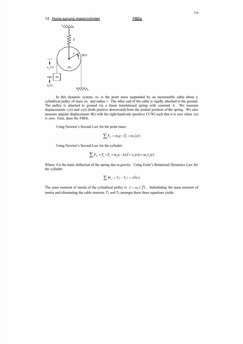
8/11/2019 Mechanism kinematics & dynamics.pdf
http://slidepdf.com/reader/full/mechanism-kinematics-dynamicspdf 216/269
216
12. Hung-sprung mass/cylinder FBDs
In this dynamic system, m1 is the point mass suspended by an inextensible cable about acylindrical pulley of mass m2 and radius r . The other end of the cable is rigidly attached to the ground.The pulley is attached to ground via a linear translational spring with constant k . We measuredisplacements x1(t ) and x2(t ) (both positive downward) from the neutral position of the spring. We also
measure angular displacement (t ) with the right-hand-rule (positive CCW) such that it is zero when x(t )is zero. First, draw the FBDs.
Using Newton’s Second Law for the point mass:
1 1 1 1( ) X F m g T m x t
Using Newton’s Second Law for the cylinder:
1 2 2 2 2 2( ( )) ( ) X F T T m g k x t m x t
Where is the static deflection of the spring due to gravity. Using Euler’s Rotational Dynamics Law forthe cylinder:
1 2 ( ) Z
M T r T r J t
The mass moment of inertia of the cylindrical pulley is 22 2 J m r . Substituting the mass moment of
inertia and eliminating the cable tensions T 1 and T 2 amongst these three equations yields
m
m
k
x (t)
r (t)
x (t)
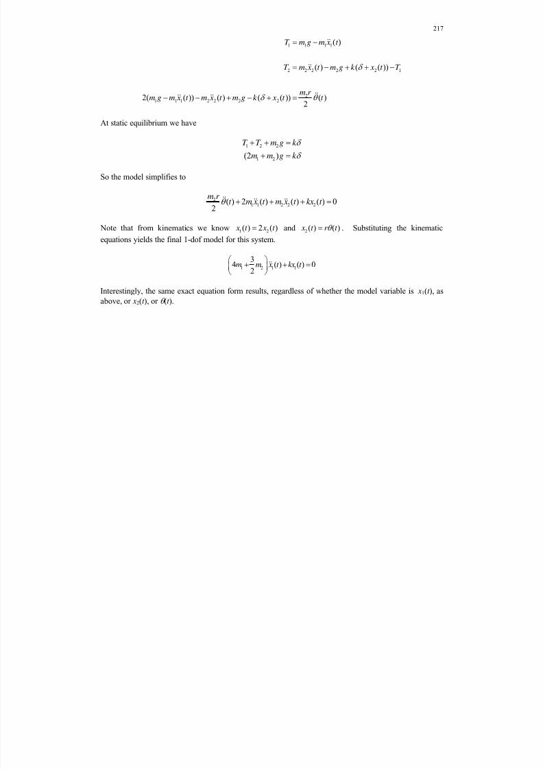
8/11/2019 Mechanism kinematics & dynamics.pdf
http://slidepdf.com/reader/full/mechanism-kinematics-dynamicspdf 217/269
217
1 1 1 1
2 2 2 2 2 1
21 1 1 2 2 2 2
( )
( ) ( ( ))
2( ( )) ( ) ( ( )) ( )2
T m g m x t
T m x t m g k x t T
m r m g m x t m x t m g k x t t
At static equilibrium we have
1 2 2
1 2(2 )
T T m g k
m m g k
So the model simplifies to
21 1 2 2 2( ) 2 ( ) ( ) ( ) 0
2
m r t m x t m x t kx t
Note that from kinematics we know 1 2( ) 2 ( ) x t x t and 2( ) ( ) x t r t . Substituting the kinematic
equations yields the final 1-dof model for this system.
1 2 1 1
34 ( ) ( ) 0
2m m x t kx t
Interestingly, the same exact equation form results, regardless of whether the model variable is x1(t ), as
above, or x2(t ), or (t ).
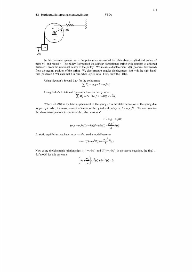
8/11/2019 Mechanism kinematics & dynamics.pdf
http://slidepdf.com/reader/full/mechanism-kinematics-dynamicspdf 218/269
218
13. Horizontally-sprung mass/cylinder FBDs
In this dynamic system, m1 is the point mass suspended by cable about a cylindrical pulley ofmass m2 and radius r . The pulley is grounded via a linear translational spring with constant k , attacheddistance a from the rotational center of the pulley. We measure displacement x(t ) (positive downward)
from the neutral position of the spring. We also measure angular displacement (t ) with the right-hand-
rule (positive CCW) such that it is zero when x(t ) is zero. First, draw the FBDs.
Using Newton’s Second Law for the point mass:
1 1 ( ) X F m g T m x t
Using Euler’s Rotational Dynamics Law for the cylinder:
( ( )) ( ) Z M Tr ka a t J t
Where ( )a t is the total displacement of the spring ( is the static deflection of the spring due
to gravity). Also, the mass moment of inertia of the cylindrical pulley is 2
2 2 J m r . We can combine
the above two equations to eliminate the cable tension T .
1 1
2
21 1
( )
( ( )) ( ( )) ( )2
T m g m x t
m r m g m x t r ka a t t
At static equilibrium we have 1m gr k a , so the model becomes
22 2
1 ( ) ( ) ( )2
m r m rx t ka t t
Now using the kinematic relationships ( ) ( ) x t r t and ( ) ( ) x t r t in the above equation, the final 1-
dof model for this system is
2 221 ( ) ( ) 0
2
mm r t ka t
m
m
k
x(t)
r (t)a

8/11/2019 Mechanism kinematics & dynamics.pdf
http://slidepdf.com/reader/full/mechanism-kinematics-dynamicspdf 219/269
219
14. Cylinder rolling in a big cylinder FBD
In this dynamic system, a cylinder of mass m and radius r rolls without slipping in a concave
cylindrical surface of radius R as shown. 1(t ) is the angular displacement of the cylinder and 2(t ) is theangular displacement of the cylinder CG from the vertical. Both angles are measured with the right-
hand-rule (positive CCW) such that they are zero when the cylinder is at static equilibrium at the bottomof the well. We define the moving X axis such that it is perpendicular to the radial direction, pointing tothe left. First, draw the FBD.
Using Newton’s Second Law for the cylinder:
2sin ( ) ( ) X f F mg t F mx t
Using Euler’s Rotational Dynamics Law for the cylinder:
1 2( ( ) ( )) Z f
M F r J t t
Note we must use the absolute angular acceleration1 2( ) ( )t t in the above equation. The mass
moment of inertia of the cylindrical pulley is 2 2 J mr . Substituting the mass moment of inertia and
eliminating the friction force F f between these two equations yields
2
2 1 2
sin ( ) ( )
sin ( ) ( ) ( ( ) ( ))2
f F mg t mx t
mr mg t mx t t t
Note that from kinematics we know2( ) ( ) ( ) x t R r t and 1 2( ) ( )t R t r . Substituting the
kinematic equations yields
2 23( ) ( ) sin ( ) 0
2 R r t g t
We apply a small angle assumption such that 2 2sin ( ) ( )t t . The final linearized 1-dof model for this
system is
2 2
3( )( ) ( ) 0
2
R r t g t
m
r
(t)
R
1
(t)2
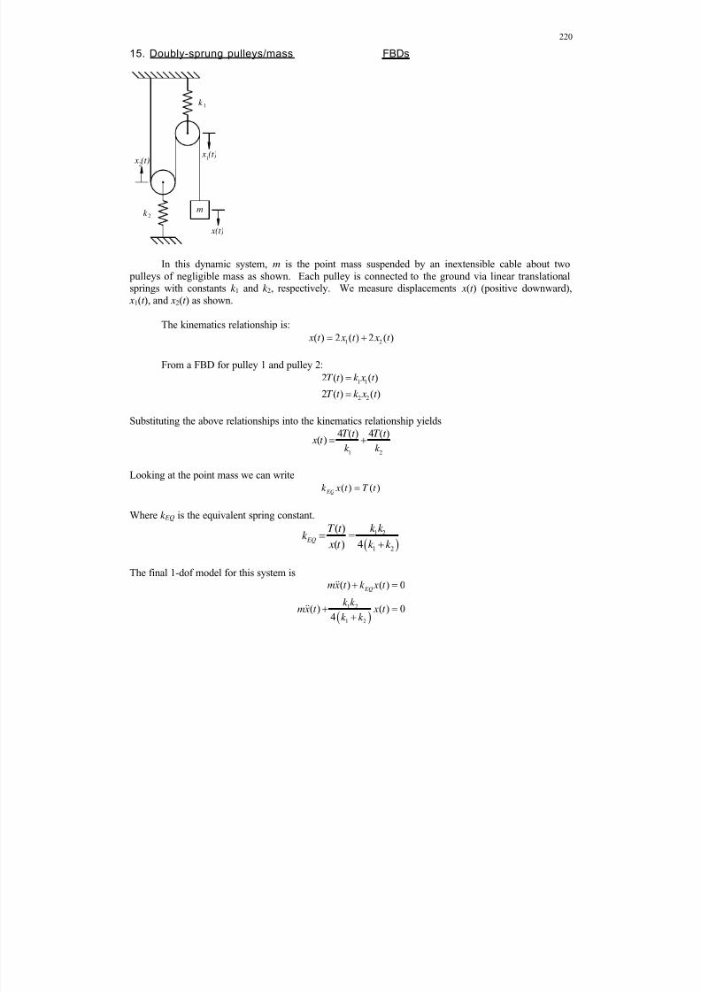
8/11/2019 Mechanism kinematics & dynamics.pdf
http://slidepdf.com/reader/full/mechanism-kinematics-dynamicspdf 220/269
220
15. Doubly-sprung pulleys/mass FBDs
In this dynamic system, m is the point mass suspended by an inextensible cable about two pulleys of negligible mass as shown. Each pulley is connected to the ground via linear translationalsprings with constants k 1 and k 2, respectively. We measure displacements x(t ) (positive downward), x1(t ), and x2(t ) as shown.
The kinematics relationship is:
1 2( ) 2 ( ) 2 ( ) x t x t x t
From a FBD for pulley 1 and pulley 2:
1 1
2 2
2 ( ) ( )
2 ( ) ( )
T t k x t
T t k x t
Substituting the above relationships into the kinematics relationship yields
1 2
4 ( ) 4 ( )( )
T t T t x t
k k
Looking at the point mass we can write
( ) ( ) EQk x t T t
Where k EQ is the equivalent spring constant.
1 2
1 2
( )
( ) 4 EQ
k k T t k x t k k
The final 1-dof model for this system is
1 2
1 2
( ) ( ) 0
( ) ( ) 04
EQmx t k x t
k k mx t x t
k k
mk
x(t)
k
x (t) x (t)
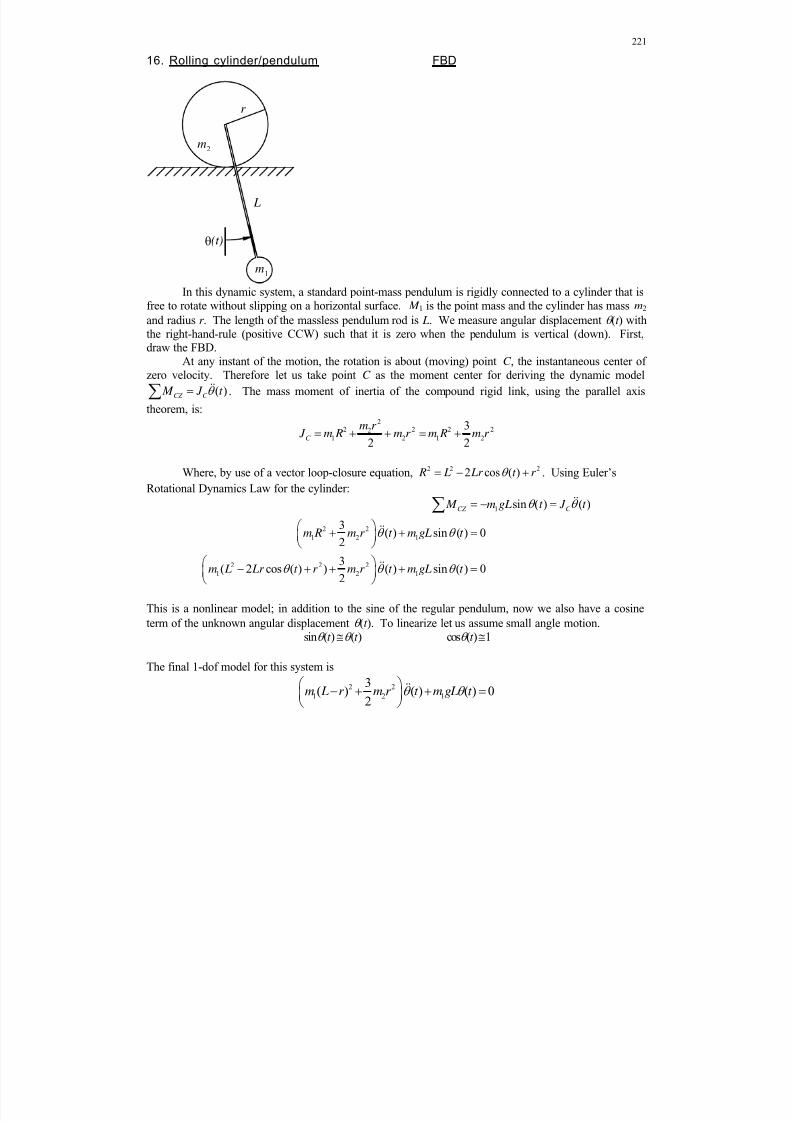
8/11/2019 Mechanism kinematics & dynamics.pdf
http://slidepdf.com/reader/full/mechanism-kinematics-dynamicspdf 221/269
221
16. Rolling cylinder/pendulum FBD
In this dynamic system, a standard point-mass pendulum is rigidly connected to a cylinder that is
free to rotate without slipping on a horizontal surface. M 1 is the point mass and the cylinder has mass m2 and radius r . The length of the massless pendulum rod is L. We measure angular displacement (t ) withthe right-hand-rule (positive CCW) such that it is zero when the pendulum is vertical (down). First,draw the FBD.
At any instant of the motion, the rotation is about (moving) point C , the instantaneous center ofzero velocity. Therefore let us take point C as the moment center for deriving the dynamic model
( )CZ C M J t . The mass moment of inertia of the compound rigid link, using the parallel axis
theorem, is:2
2 2 2 221 2 1 2
3
2 2C
m r J m R m r m R m r
Where, by use of a vector loop-closure equation, 2 2 22 cos ( ) R L Lr t r . Using Euler’s
Rotational Dynamics Law for the cylinder:
1
2 2
1 2 1
2 2 2
1 2 1
sin ( ) ( )
3( ) sin ( ) 0
2
3( 2 cos ( ) ) ( ) sin ( ) 0
2
CZ C M m gL t J t
m R m r t m gL t
m L Lr t r m r t m gL t
This is a nonlinear model; in addition to the sine of the regular pendulum, now we also have a cosineterm of the unknown angular displacement (t ). To linearize let us assume small angle motion.
sin ( ) ( )t t
cos ( ) 1t
The final 1-dof model for this system is
2 2
1 2 1
3( ) ( ) ( ) 0
2m L r m r t m gL t
m
L
(t)
1
m2
r
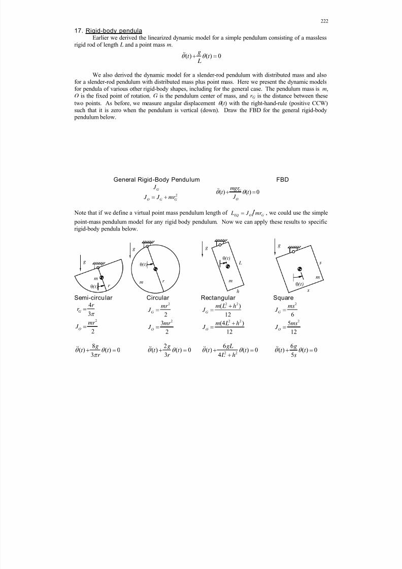
8/11/2019 Mechanism kinematics & dynamics.pdf
http://slidepdf.com/reader/full/mechanism-kinematics-dynamicspdf 222/269
222
17. Rigid-body pendula Earlier we derived the linearized dynamic model for a simple pendulum consisting of a massless
rigid rod of length L and a point mass m.
( ) ( ) 0g
t t L
We also derived the dynamic model for a slender-rod pendulum with distributed mass and alsofor a slender-rod pendulum with distributed mass plus point mass. Here we present the dynamic modelsfor pendula of various other rigid-body shapes, including for the general case. The pendulum mass is m,O is the fixed point of rotation, G is the pendulum center of mass, and r G is the distance between these
two points. As before, we measure angular displacement (t ) with the right-hand-rule (positive CCW)such that it is zero when the pendulum is vertical (down). Draw the FBD for the general rigid-body pendulum below.
General Rigid-Body Pendulum FBD
2
G
O G G
J
J J mr ( ) ( ) 0G
O
mgr t t
J
Note that if we define a virtual point mass pendulum length of EQ O G
L J mr , we could use the simple
point-mass pendulum model for any rigid body pendulum. Now we can apply these results to specific
rigid-body pendula below.
Semi-circular Circular Rectangular Square
2
43
2
G
O
r r
mr J
2
2
2
3
2
G
O
mr J
mr J
2 2
2 2
( )12
(4 )
12
G
O
m L h J
m L h J
2
2
6
5
12
G
O
ms J
ms J
8( ) ( ) 0
3
gt t
r
2( ) ( ) 0
3
gt t
r
2 2
6( ) ( ) 0
4
gLt t
L h
6( ) ( ) 0
5
gt t
s
r
g
(t)
m
r
g
(t)
m
h
g
(t)
m
L
g
(t)
m
s
s
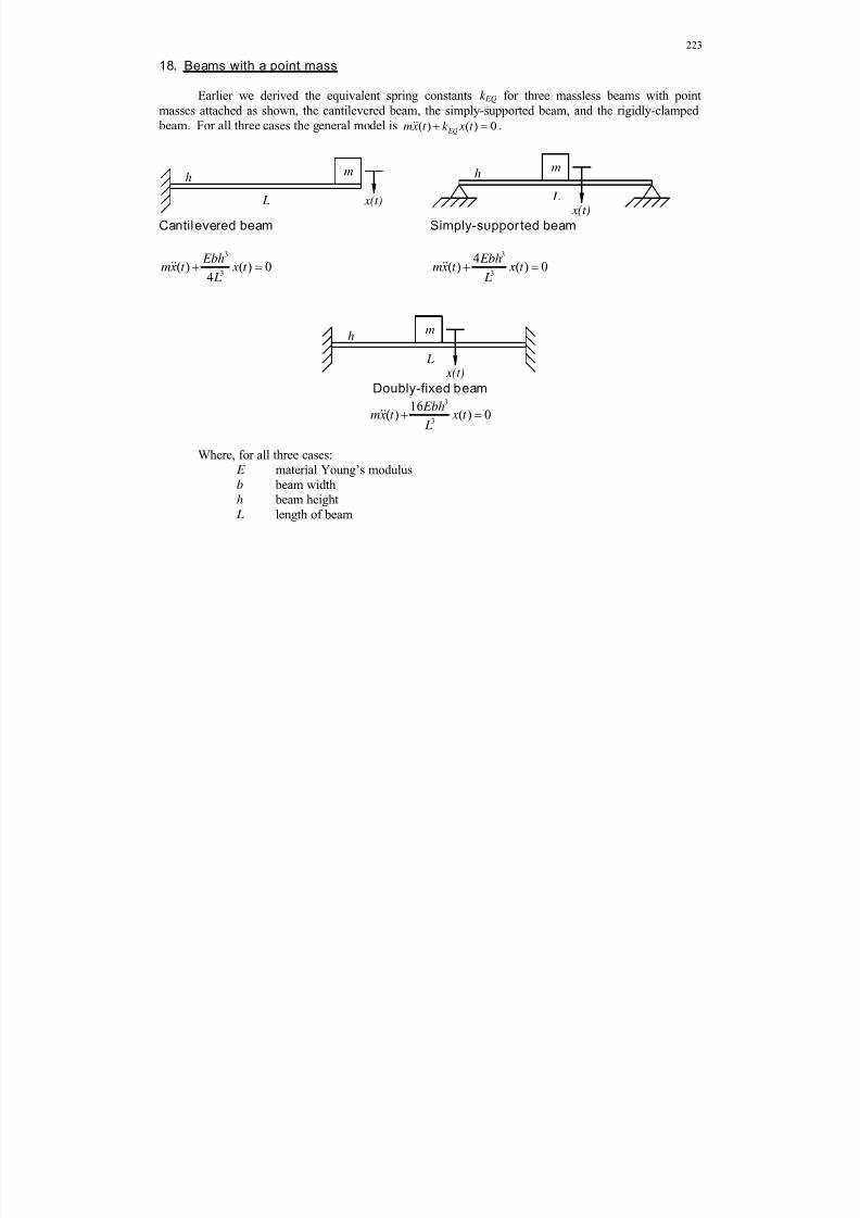
8/11/2019 Mechanism kinematics & dynamics.pdf
http://slidepdf.com/reader/full/mechanism-kinematics-dynamicspdf 223/269
223
18. Beams with a point mass
Earlier we derived the equivalent spring constants k EQ for three massless beams with pointmasses attached as shown, the cantilevered beam, the simply-supported beam, and the rigidly-clamped beam. For all three cases the general model is ( ) ( ) 0 EQ
mx t k x t .
Cantilevered beam Simply-supported beam
3
3( ) ( ) 0
4
Ebhmx t x t
L
3
3
4( ) ( ) 0
Ebhmx t x t
L
Doubly-fixed beam3
3
16( ) ( ) 0
Ebhmx t x t
L
Where, for all three cases: E material Young’s modulusb beam widthh beam height L length of beam
m
L x(t)
hm
L x(t)
h
m
L x(t)
h
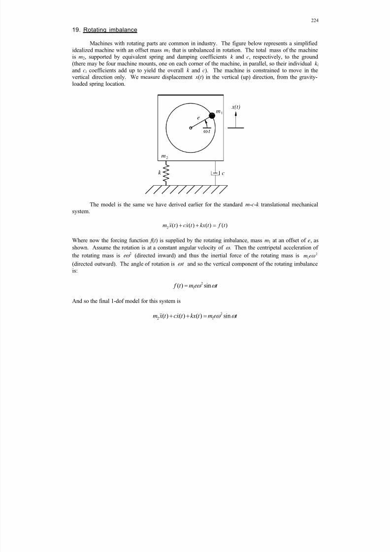
8/11/2019 Mechanism kinematics & dynamics.pdf
http://slidepdf.com/reader/full/mechanism-kinematics-dynamicspdf 224/269
224
19. Rotating imbalance
Machines with rotating parts are common in industry. The figure below represents a simplifiedidealized machine with an offset mass m1 that is unbalanced in rotation. The total mass of the machineis m2, supported by equivalent spring and damping coefficients k and c, respectively, to the ground(there may be four machine mounts, one on each corner of the machine, in parallel, so their individual k i and ci coefficients add up to yield the overall k and c). The machine is constrained to move in thevertical direction only. We measure displacement x(t ) in the vertical (up) direction, from the gravity-loaded spring location.
The model is the same we have derived earlier for the standard m-c-k translational mechanicalsystem.
2 ( ) ( ) ( ) ( )m x t cx t kx t f t
Where now the forcing function f (t ) is supplied by the rotating imbalance, mass m1 at an offset of e, as
shown. Assume the rotation is at a constant angular velocity of . Then the centripetal acceleration of
the rotating mass is 2e (directed inward) and thus the inertial force of the rotating mass is 2
1m e
(directed outward). The angle of rotation is t and so the vertical component of the rotating imbalanceis:
2
1( ) sin f t me t
And so the final 1-dof model for this system is
2
2 1( ) ( ) ( ) sinm x t cx t kx t m e t
m1
m2
k c
x(t)
e
t
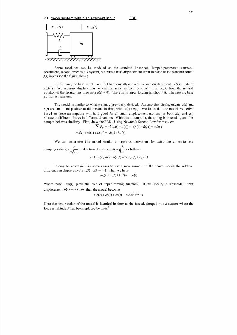
8/11/2019 Mechanism kinematics & dynamics.pdf
http://slidepdf.com/reader/full/mechanism-kinematics-dynamicspdf 225/269

8/11/2019 Mechanism kinematics & dynamics.pdf
http://slidepdf.com/reader/full/mechanism-kinematics-dynamicspdf 226/269
226
21. Horizontal sprung pendulum FBD
In the figure above, a horizontal simple pendulum has a point mass on the end of a massless rigidrod of length a. The rod extends by length b to the other side to connect to the ground through a linear
translational spring with constant k . We measure angular displacement (t ) with the right-hand-rule(positive CCW) such that it is zero when the pendulum is horizontal. We further measure displacementvariable x(t ) as the extension/compression of the spring as shown. First, draw the FBD.
Using Euler’s Rotational Dynamics Law for the pendulum:
cos ( ) ( ( )) ( ) Z M mga t bk x t J t
Where ( ) x t is the total displacement of the spring ( is the static deflection of the spring in
tension due to gravity). Also, the mass moment of inertia of the pendulum about the axis of rotation is2
J ma .
2 ( ) ( ( )) cos ( ) 0ma t bk x t mga t
This is a nonlinear model, due to the cosine term of the unknown angular displacement (t ). To
linearize let us assume small angle motion cos ( ) 1t .
2 ( ) ( ( )) 0ma t bk x t mga
At static equilibrium we have mga kb , so the simplified model for this system is
2 ( ) ( ) 0ma t bkx t
For a small displacement x(t ) the approximation ( ) sin ( ) x t b t holds good. Once again assuming
small angle motion, to linearize we use sin ( ) ( )t t , so the final 1-dof model for this system is
2 2( ) ( ) 0ma t kb t
m
k
a
(t)
x(t)b
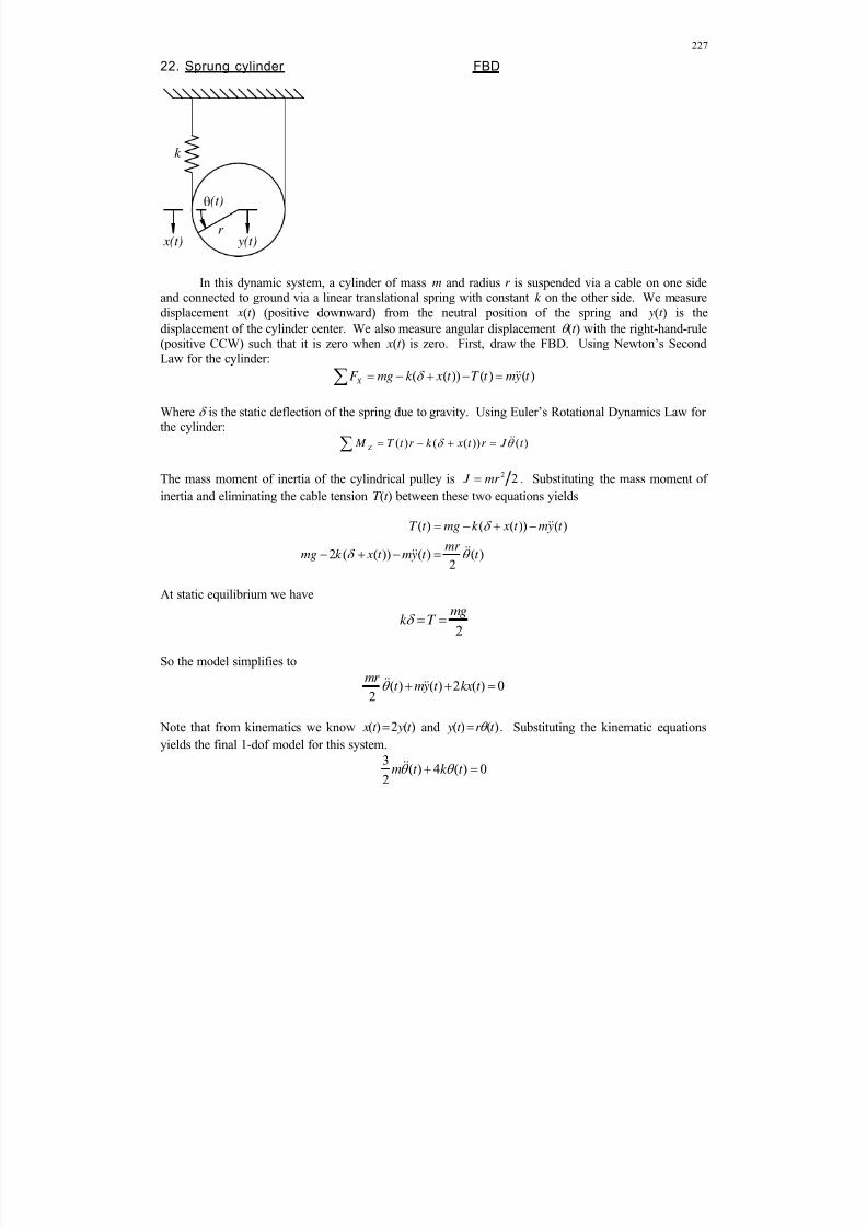
8/11/2019 Mechanism kinematics & dynamics.pdf
http://slidepdf.com/reader/full/mechanism-kinematics-dynamicspdf 227/269
227
22. Sprung cylinder FBD
In this dynamic system, a cylinder of mass m and radius r is suspended via a cable on one sideand connected to ground via a linear translational spring with constant k on the other side. We measuredisplacement x(t ) (positive downward) from the neutral position of the spring and y(t ) is the
displacement of the cylinder center. We also measure angular displacement (t ) with the right-hand-rule(positive CCW) such that it is zero when x(t ) is zero. First, draw the FBD. Using Newton’s SecondLaw for the cylinder:
( ( )) ( ) ( ) X F mg k x t T t my t
Where is the static deflection of the spring due to gravity. Using Euler’s Rotational Dynamics Law forthe cylinder:
( ) ( ( )) ( ) Z
M T t r k x t r J t
The mass moment of inertia of the cylindrical pulley is 2 2 J mr . Substituting the mass moment of
inertia and eliminating the cable tension T (t ) between these two equations yields
( ) ( ( )) ( )
2 ( ( )) ( ) ( )2
T t mg k x t my t
mr mg k x t my t t
At static equilibrium we have
2
mgk T
So the model simplifies to
( ) ( ) 2 ( ) 02
mr t my t kx t
Note that from kinematics we know ( ) 2 ( ) x t y t and ( ) ( ) y t r t . Substituting the kinematic equations
yields the final 1-dof model for this system.
3( ) 4 ( ) 0
2m t k t
k
x(t)r
(t)
y(t)

8/11/2019 Mechanism kinematics & dynamics.pdf
http://slidepdf.com/reader/full/mechanism-kinematics-dynamicspdf 228/269
228

8/11/2019 Mechanism kinematics & dynamics.pdf
http://slidepdf.com/reader/full/mechanism-kinematics-dynamicspdf 229/269
229
23. Vertical sprung pendulum with damping FBD
In the figure above, a simple pendulum rotating about point O has a point mass on the end of amassless rigid rod of length L. The rod extends by length b to the other side of point O to connect to theground through a horizontal linear translational spring with constant k . We measure angular
displacement (t ) with the right-hand-rule (positive CCW) such that it is zero when the pendulum is
vertical. We further measure displacement variable ( ) ( )b x t b t as the compression/extension of the
spring as shown. A viscous dashpot is connected by length a down along the rod to provide damping,
with velocity variable ( ) ( )a x t a t . First, draw the FBD.
Using Euler’s Rotational Dynamics Law for the pendulum:
sin ( ) ( ) cos ( ) ( ) cos ( ) ( )OZ M mgL t kb t b t ca t a t J t
The mass moment of inertia of the pendulum about the axis of rotation is 2 J mL .
2 2 2( ) sin ( ) ( )cos ( ) ( )cos ( ) 0mL t mgL t kb t t ca t t
This is a nonlinear model; in addition to the sine of the regular pendulum, now we also have a cosine
term of the unknown angular displacement (t ). To linearize let us assume small angle motion.
sin ( ) ( )t t
cos ( ) 1t
Then the final 1-dof model for this system is
2 2 2( ) ( ) ( ) ( ) 0mL t ca t mgL kb t
m
k
L
(t)
ca
b
x (t)b
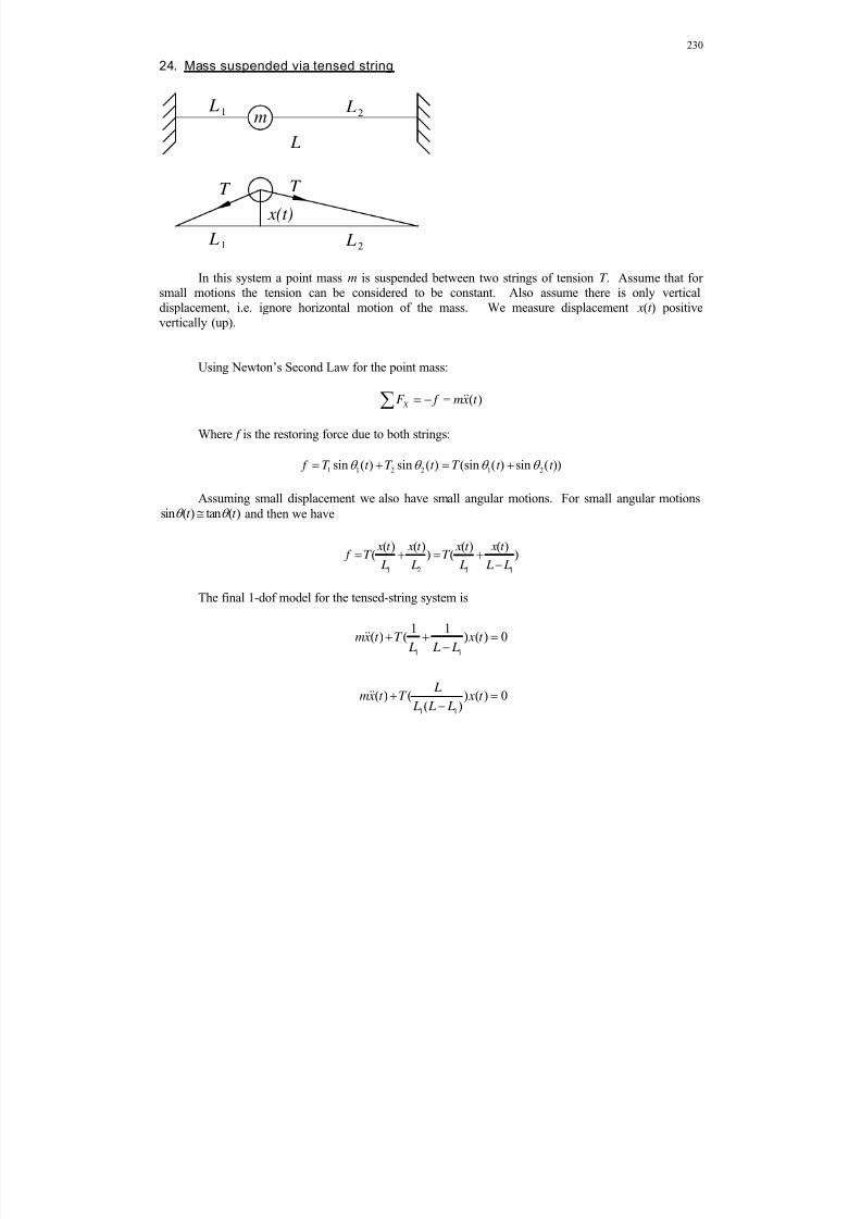
8/11/2019 Mechanism kinematics & dynamics.pdf
http://slidepdf.com/reader/full/mechanism-kinematics-dynamicspdf 230/269
230
24. Mass suspended via tensed string
In this system a point mass m is suspended between two strings of tension T . Assume that forsmall motions the tension can be considered to be constant. Also assume there is only verticaldisplacement, i.e. ignore horizontal motion of the mass. We measure displacement x(t ) positivevertically (up).
Using Newton’s Second Law for the point mass:
( ) X F f mx t
Where f is the restoring force due to both strings:
1 1 2 2 1 2sin ( ) sin ( ) (sin ( ) sin ( )) f T t T t T t t
Assuming small displacement we also have small angular motions. For small angular motionssin ( ) tan ( )t t and then we have
1 2 1 1
( ) ( ) ( ) ( )( ) ( ) x t x t x t x t
f T T L L L L L
The final 1-dof model for the tensed-string system is
1 1
1 1
1 1( ) ( ) ( ) 0
( ) ( ) ( ) 0( )
mx t T x t L L L
Lmx t T x t
L L L
m
L
L 1 L 2
L 1 L 2
x(t)
T T
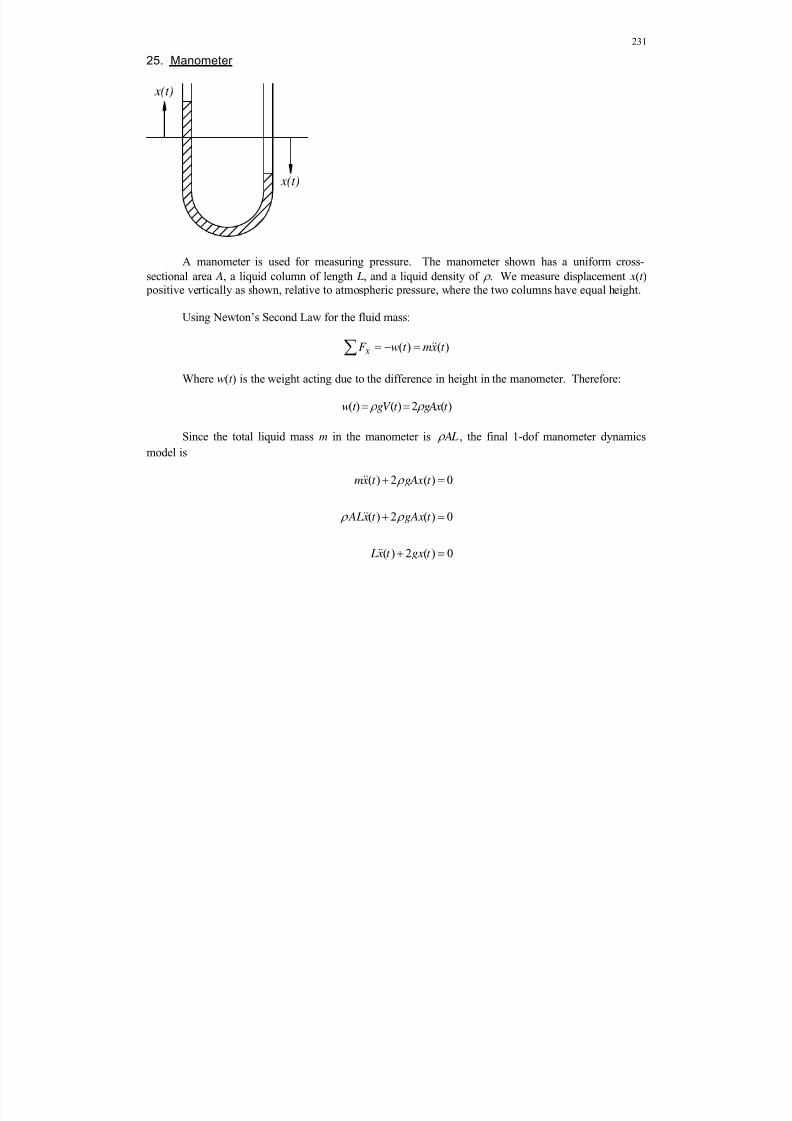
8/11/2019 Mechanism kinematics & dynamics.pdf
http://slidepdf.com/reader/full/mechanism-kinematics-dynamicspdf 231/269
231
25. Manometer
A manometer is used for measuring pressure. The manometer shown has a uniform cross-
sectional area A, a liquid column of length L, and a liquid density of . We measure displacement x(t ) positive vertically as shown, relative to atmospheric pressure, where the two columns have equal height.
Using Newton’s Second Law for the fluid mass:
( ) ( ) X F w t mx t
Where w(t ) is the weight acting due to the difference in height in the manometer. Therefore:
( ) ( ) 2 ( )w t gV t gAx t
Since the total liquid mass m in the manometer is AL , the final 1-dof manometer dynamics
model is
( ) 2 ( ) 0
( ) 2 ( ) 0
( ) 2 ( ) 0
mx t gAx t
ALx t gAx t
Lx t gx t
x(t)
x(t)
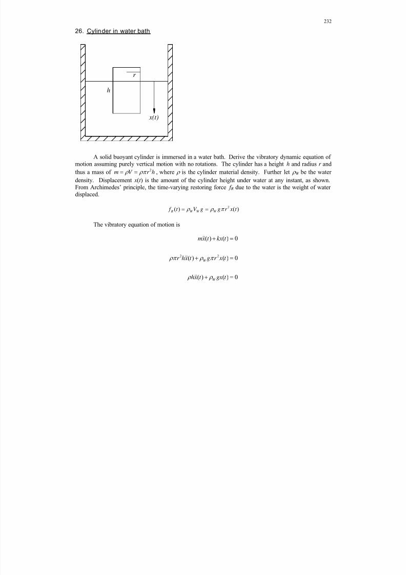
8/11/2019 Mechanism kinematics & dynamics.pdf
http://slidepdf.com/reader/full/mechanism-kinematics-dynamicspdf 232/269
232
26. Cylinder in water bath
A solid buoyant cylinder is immersed in a water bath. Derive the vibratory dynamic equation ofmotion assuming purely vertical motion with no rotations. The cylinder has a height h and radius r and
thus a mass of 2m V r h , where is the cylinder material density. Further let W be the water
density. Displacement x(t ) is the amount of the cylinder height under water at any instant, as shown.From Archimedes’ principle, the time-varying restoring force f R due to the water is the weight of waterdisplaced.
2( ) ( ) R W W W f t V g g r x t
The vibratory equation of motion is
2 2
( ) ( ) 0
( ) ( ) 0
( ) ( ) 0
W
W
mx t kx t
r hx t g r x t
hx t gx t
x(t)
h
r

8/11/2019 Mechanism kinematics & dynamics.pdf
http://slidepdf.com/reader/full/mechanism-kinematics-dynamicspdf 233/269
233
27. Human skeletal muscle model
This section presents a common single skeletal muscle dynamics model, including the figure,equations, state-space form, and simulations. This is a vibrational model, included for completeness, toshow one type of engineering mechanics modeling for muscles. In this class we will generally treat theeffect of muscles more simply, i.e. as simple cables in tension with no mass, spring constants, ordynamics of their own.
The model in this section was suggested by Dr. Scott Hooper (OU Biological Sciences) and theequations were derived and the simulations performed by Elvedin Kljuno (OU Fulbright Scholar fromBosnia). Dr. Hooper uses this model to study neural muscular control in the stomachs of lobsters, but hesays it can be scaled to adequately model skeletal muscle in many animals, including humans.
The skeletal muscle vibrational dynamics model is shown below. The lumped mass m representsthe load the muscle is lifting vs. gravity g. The muscle itself is represented by linear elastic springstiffness k 1, in parallel with linear elastic spring stiffness k 2 that is in series with linear dissipativedashpot b. The absolute displacement of the dashpot end and the muscle end are measured bycoordinates x and y, respectively. Lengths L1R and L2R (not shown) are the resting lengths (not stretched
by gravity) of springs 1 and 2, respectively. In vibrations it is more common to measure change indisplacements relative to the gravity-stretched position, but biologists need to include the absolute springlengths as well. The actuator F A represents the contractile element of the muscle and F m is the force
generated by the muscle. Note: this derivation assumes zero pennation angle, i.e. zero angle betweenthe muscle fibers and the tendons.
Dynamic Skeletal Muscle Diagram

8/11/2019 Mechanism kinematics & dynamics.pdf
http://slidepdf.com/reader/full/mechanism-kinematics-dynamicspdf 234/269
234
The parallel elastic component k 1, provided by the muscle membranes, gives spring resistancewhen passively stretched. The series elastic component k 2 represents the tendons, storing elasticenergy when a muscle is stretched. The tension-generating contractile effect of the sarcomeres,modeled by actuator force F A, is in parallel with the membranes and in series with the tendons.
From the left figure below, the equation for the left spring is:
1 1R 1
( )k y L F (1)
From the right figure above, the equations for the right spring and dashpot are:
2 2R 2
2 A
( )k y x L F
bx F F
(2, 3)
From the FBD shown below, the dynamics equation for the mass is obtained using Newton’s Secondlaw:
1 2 m
vert vert F ma
F F F mg my
(4)

8/11/2019 Mechanism kinematics & dynamics.pdf
http://slidepdf.com/reader/full/mechanism-kinematics-dynamicspdf 235/269
235
Substituting (1) and (2) into (4), and also substituting (2) into (3) yields the following coupledsecond/first order linear vibrational dynamics model for skeletal muscle.
1 1R 2 2R m
2 2R A
( ) ( )
( )
my k y L k y x L mg F
bx k y x L F
(5, 6)
Equations (5, 6) can be written in the following form:
2 m1 2 1 1R 2 2R
2 2 A 22R
1 1( ) ( )
k F y k k y x k L k L g
m m m m
k k F k x x y L
b b b b
(7, 8)
As mentioned above, (7, 8) can be simplified by choosing more adequate coordinates that willmeasure the deviation from the static position only. The form shown above is formed intentionally for
biological systems, using absolute coordinates and initial spring lengths.
The system of differential equations (7, 8) can be solved for coordinates x and y as functions oftime given time functions for F A and F m. In the case of a simple form of F A and F m the solution could be found using reduction and decoupling by a formation of a single third-order linear ordinarydifferential equation.
2 1 2 1 2 21 1
( )( )( ) ( ) ( ) ( ) ( ( ) ( ) )m
A m R
F t k k k k k k y t y t y t y t F t F t mg k L
b m mb m mb
(9)
Equation (9) can be solved for y(t ) which is then substituted into (8) to directly solve for x(t ).

8/11/2019 Mechanism kinematics & dynamics.pdf
http://slidepdf.com/reader/full/mechanism-kinematics-dynamicspdf 236/269
236
Common Model Features
Considering all vibrational models we have derived, including the many cases in this section,some general comments can be made about all models.
1.
When gathering the unknown and its time derivatives on one side of the ODE, there willnever be a change in sign amongst these terms; generally they will all be positive.
2. The effect of gravity always cancels out. That is, any mg static weight terms will load thespring with a static deflection and these terms always subtract out of the final ODE.
3. As always, the resulting units must be consistent. This is a good check to perform on yourresulting model.
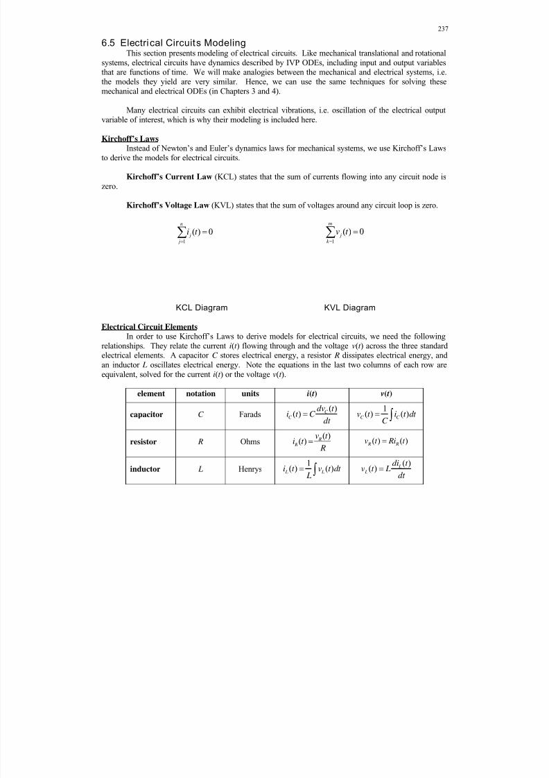
8/11/2019 Mechanism kinematics & dynamics.pdf
http://slidepdf.com/reader/full/mechanism-kinematics-dynamicspdf 237/269
237
6.5 Electrical Circuits ModelingThis section presents modeling of electrical circuits. Like mechanical translational and rotational
systems, electrical circuits have dynamics described by IVP ODEs, including input and output variablesthat are functions of time. We will make analogies between the mechanical and electrical systems, i.e.the models they yield are very similar. Hence, we can use the same techniques for solving thesemechanical and electrical ODEs (in Chapters 3 and 4).
Many electrical circuits can exhibit electrical vibrations, i.e. oscillation of the electrical outputvariable of interest, which is why their modeling is included here.
Kirchoff’s Laws
Instead of Newton’s and Euler’s dynamics laws for mechanical systems, we use Kirchoff’s Lawsto derive the models for electrical circuits.
Kirchoff’s Current Law (KCL) states that the sum of currents flowing into any circuit node iszero.
Kirchoff’s Voltage Law (KVL) states that the sum of voltages around any circuit loop is zero.
1
( ) 0n
j
j
i t
1
( ) 0m
j
k
v t
KCL Diagram KVL Diagram
Electrical Circuit Elements
In order to use Kirchoff’s Laws to derive models for electrical circuits, we need the followingrelationships. They relate the current i(t ) flowing through and the voltage v(t ) across the three standardelectrical elements. A capacitor C stores electrical energy, a resistor R dissipates electrical energy, andan inductor L oscillates electrical energy. Note the equations in the last two columns of each row areequivalent, solved for the current i(t ) or the voltage v(t ).
element notation units i( t) v( t)
capacitor C Farads
( )( ) C
C
dv t i t C
dt
1
( ) ( )C C v t i t dt
C
resistor R Ohms
( )( ) R
R
v t i t
R ( ) ( ) R Rv t Ri t
inductor L Henrys
1( ) ( )
L Li t v t dt L
( )
( ) L L
di t v t L
dt

8/11/2019 Mechanism kinematics & dynamics.pdf
http://slidepdf.com/reader/full/mechanism-kinematics-dynamicspdf 238/269
238
Additional Electrical Circuit Variables
In some electrical circuit modeling you may encounter two more variable types, electrical charge
and electrical flux. As shown in Dr. Bob’s on-line Atlas of Models and Transfer Functions,
www.ohio.edu/people/williar4/html/PDF/ModelTFAtlas.pdf
electrical charge q(t ) is the time integral of current i(t ) and electrical flux (t ) is the time integral of
voltage v(t ).
( ) ( )q t i t dt
( ) ( )t v t dt
Convention for Electron Flow
When early electricity experimenters and early electrical engineer pioneers established the
convention for the flow of electrons composing current, they got it backwards. This error persists to thisday, because it really doesn’t matter in the equations.
xkcd.com

8/11/2019 Mechanism kinematics & dynamics.pdf
http://slidepdf.com/reader/full/mechanism-kinematics-dynamicspdf 239/269
239
Current-Driven Parallel R- L-C Electrical Circuit Model
The system diagram for the current-driven parallel R- L-C electrical circuit is shown below. Theinput is current i(t ), and the output is voltage v(t ). The voltage across the current generator, the resistor R, the inductor L, and the capacitor C are all identical, v(t ).
Parallel R-L-C Circuit Diagram
Using Kirchoff’s Current Law (the sum of currents into any circuit node is zero), we have:
( ) ( ) ( ) ( ) 0
( ) ( ) ( ) ( )
R L C
C R L
i t i t i t i t
i t i t i t i t
Substituting the current through each element as a function of voltage v(t ) from the previous table, weobtain the model for the current-driven parallel R- L-C circuit.
( ) 1 1( ) ( ) ( )
dv t C v t v t dt i t
dt R L
This model is a linear, lumped-parameter, constant-coefficient, integro-differential equation. It issecond-order, since, although the highest derivative order is first-order, there are two time differentiationsteps between the integral and the first derivative. This equation is written in standard form, where theoutput variable v(t ) appears with its derivative and integral on the left-hand-side and the input forcingfunction i(t ) appears on the right-hand-side of the equation. The external current input is i(t ) (amps) andthe output is voltage v(t ) (volts).
i(t) R L C v(t)
+
-
i (t) L
i (t) R
i (t)C
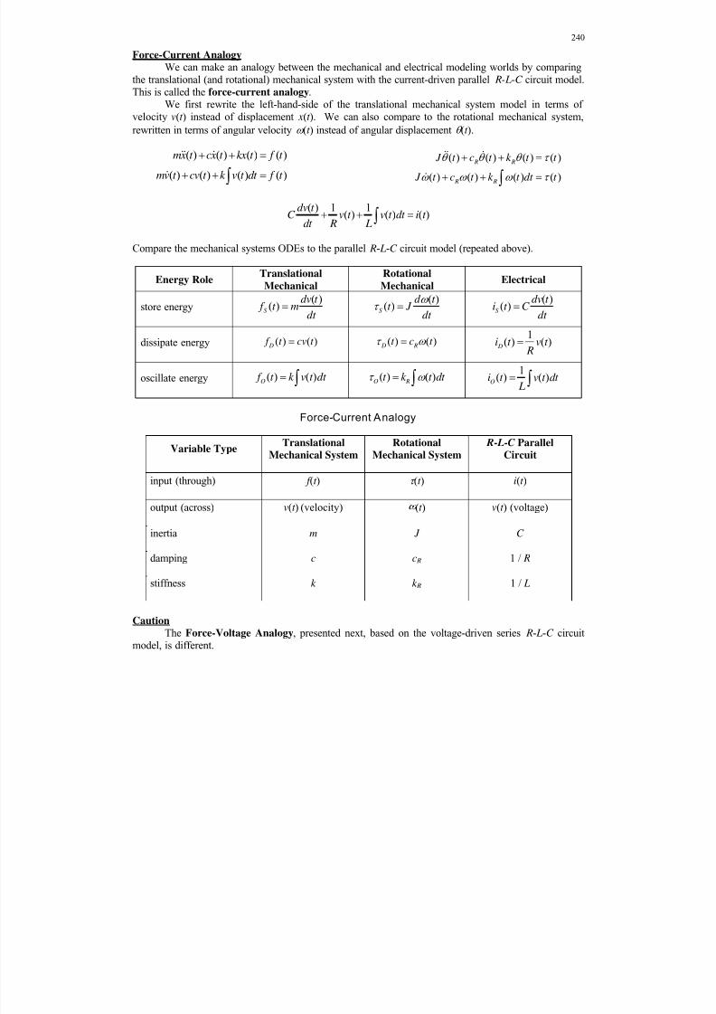
8/11/2019 Mechanism kinematics & dynamics.pdf
http://slidepdf.com/reader/full/mechanism-kinematics-dynamicspdf 240/269
240
Force-Current Analogy
We can make an analogy between the mechanical and electrical modeling worlds by comparingthe translational (and rotational) mechanical system with the current-driven parallel R- L-C circuit model.This is called the force-current analogy.
We first rewrite the left-hand-side of the translational mechanical system model in terms ofvelocity v(t ) instead of displacement x(t ). We can also compare to the rotational mechanical system,
rewritten in terms of angular velocity (t ) instead of angular displacement (t ).
( ) ( ) ( ) ( )
( ) ( ) ( ) ( )
mx t cx t kx t f t
mv t cv t k v t dt f t
( ) ( ) ( ) ( )
( ) ( ) ( ) ( )
R R
R R
J t c t k t t
J t c t k t dt t
( ) 1 1( ) ( ) ( )
dv t C v t v t dt i t
dt R L
Compare the mechanical systems ODEs to the parallel R- L-C circuit model (repeated above).
Energy Role TranslationalMechanical
RotationalMechanical
Electrical
store energy( )
( )S
dv t f t m
dt
( )( )
S
d t t J
dt
( )( )
S
dv t i t C
dt
dissipate energy ( ) ( ) D f t cv t ( ) ( ) D R
t c t 1
( ) ( ) Di t v t
R
oscillate energy ( ) ( )O f t k v t dt ( ) ( )
O Rt k t dt 1
( ) ( )Oi t v t dt
L
Force-Current Analogy
Variable TypeTranslational
Mechanical System
Rotational
Mechanical System
R- L-C Parallel
Circuit
input (through) f (t ) (t ) i(t )
output (across) v(t ) (velocity) (t ) v(t ) (voltage)
inertia m J C
damping c c R 1 / R
stiffness k k R 1 / L
Caution The Force-Voltage Analogy, presented next, based on the voltage-driven series R- L-C circuit
model, is different.

8/11/2019 Mechanism kinematics & dynamics.pdf
http://slidepdf.com/reader/full/mechanism-kinematics-dynamicspdf 241/269
241

8/11/2019 Mechanism kinematics & dynamics.pdf
http://slidepdf.com/reader/full/mechanism-kinematics-dynamicspdf 242/269
242
Voltage-Driven Series R- L-C Electrical Circuit Model
The system diagram for the voltage-driven series R- L-C electrical circuit is shown below. Theinput is voltage v(t ), and the output is current i(t ). The current i(t ) flowing through all elements is thesame. The input voltage source v(t ) increases as shown negative to positive; the voltage drops acrosseach of the circuit elements, positive to negative in each case.
Series R-L-C Circuit Diagram
Using Kirchoff’s Voltage Law (the sum of voltages around the circuit loop is zero), we have:
( ) ( ) ( ) ( ) 0
( ) ( ) ( ) ( )
R L C
L R C
v t v t v t v t
v t v t v t v t
Substituting the voltage drop across each element as a function of current i(t) from the first table in thissection, we obtain the model for the voltage-driven series R- L-C circuit.
( ) 1( ) ( ) ( )
di t L Ri t i t dt v t dt C
This model is a linear, lumped-parameter, constant-coefficient, integro-differential equation. Again, it issecond-order since there are two time differentiation steps between the integral and the first derivative.This equation is written in standard form, where the output variable i(t ) appears with its derivative andintegral on the left-hand-side and the input forcing function v(t ) appears on the right-hand-side of theequation. The external input is voltage v(t ) (volts) and the output is current i(t ) (amps).
v(t) L
R
+
-i(t)
C

8/11/2019 Mechanism kinematics & dynamics.pdf
http://slidepdf.com/reader/full/mechanism-kinematics-dynamicspdf 243/269
243
Force-Voltage Analogy
We can make a different analogy between the mechanical and electrical modeling worlds bycomparing the translational (and rotational) mechanical system with the voltage-driven series R- L-C circuit model. This is called the force-voltage analogy.
We again use the translational and rotational mechanical system models, rewritten in terms of
velocity v(t ) instead of displacement x(t ) and rewritten in terms of angular velocity (t ) instead of
angular displacement (t ).
( ) ( ) ( ) ( )
( ) ( ) ( ) ( )
mx t cx t kx t f t
mv t cv t k v t dt f t
( ) ( ) ( ) ( )
( ) ( ) ( ) ( )
R R
R R
J t c t k t t
J t c t k t dt t
( ) 1( ) ( ) ( )
di t L Ri t i t dt v t
dt C
Force-Voltage Analogy
Variable TypeTranslational
Mechanical System
Rotational
Mechanical System
R- L-C Series
Circuit
input (through) f (t ) (t ) v(t ) (voltage)
output (across) v(t ) (velocity) (t ) i(t )
inertia m J L
damping c c R R
stiffness k k R 1/C
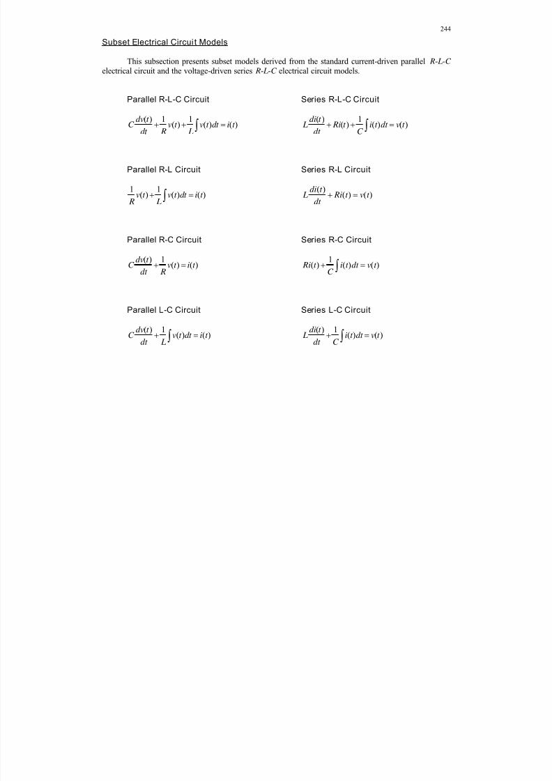
8/11/2019 Mechanism kinematics & dynamics.pdf
http://slidepdf.com/reader/full/mechanism-kinematics-dynamicspdf 244/269
244
Subset Electrical Circui t Models
This subsection presents subset models derived from the standard current-driven parallel R- L-C electrical circuit and the voltage-driven series R- L-C electrical circuit models.
Parallel R-L-C Circuit Series R-L-C Circuit
( ) 1 1( ) ( ) ( )
dv t C v t v t dt i t
dt R L
( ) 1( ) ( ) ( )
di t L Ri t i t dt v t
dt C
Parallel R-L Circuit Series R-L Circuit
1 1( ) ( ) ( )v t v t dt i t
R L
( )( ) ( )
di t L Ri t v t
dt
Parallel R-C Circuit Series R-C Circuit
( ) 1( ) ( )
dv t C v t i t
dt R
1( ) ( ) ( ) Ri t i t dt v t
C
Parallel L-C Circuit Series L-C Circuit
( ) 1( ) ( )
dv t C v t dt i t
dt L
( ) 1( ) ( )
di t L i t dt v t
dt C
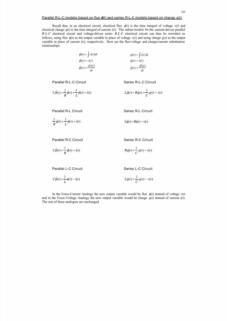
8/11/2019 Mechanism kinematics & dynamics.pdf
http://slidepdf.com/reader/full/mechanism-kinematics-dynamicspdf 245/269
245
Parallel R-L-C models based on flux (t) and series R-L-C models based on charge q(t)
Recall that, in an electrical circuit, electrical flux (t ) is the time integral of voltage v(t ) andelectrical charge q(t ) is the time integral of current i(t ). The subset models for the current-driven parallel R- L-C electrical circuit and voltage-driven series R- L-C electrical circuit can thus be rewritten as
follows, using flux (t ) as the output variable in place of voltage v(t ) and using charge q(t ) as the output
variable in place of current i(t ), respectively. Here are the flux/voltage and charge/current substitutionrelationships.
( ) ( )
( ) ( )
( )( )
t v t dt
t v t
dv t t
dt
( ) ( )
( ) ( )
( )( )
q t i t dt
q t i t
di t q t
dt
Parallel R-L-C Circuit Series R-L-C Circuit
1 1( ) ( ) ( ) ( )C t t t i t
R L
1( ) ( ) ( ) ( ) Lq t Rq t q t v t
C
Parallel R-L Circuit Series R-L Circuit
1 1( ) ( ) ( )t t i t
R L
( ) ( ) ( ) Lq t Rq t v t
Parallel R-C Circuit Series R-C Circuit
1( ) ( ) ( )C t t i t
R
1( ) ( ) ( ) Rq t q t v t
C
Parallel L-C Circuit Series L-C Circuit
1( ) ( ) ( )C t t i t
L
1( ) ( ) ( ) Lq t q t v t
C
In the Force-Current Analogy the new output variable would be flux (t ) instead of voltage v(t )and in the Force-Voltage Analogy the new output variable would be charge q(t ) instead of current i(t ).The rest of these analogies are unchanged.

8/11/2019 Mechanism kinematics & dynamics.pdf
http://slidepdf.com/reader/full/mechanism-kinematics-dynamicspdf 246/269
246
6.6 Multi-dof Vibrational Systems Models
This chapter presents some mechanical system models for systems with greater than one degree-of-freedom (dof). For multiple independent masses, draw a free-body diagram (FBD) for each mass andderive an ODE using Newton’s Second Law or Euler’s Rotational Dynamics Law. Generally there will be one second-order ODE for each independent mass. Normally the resulting set of n ODEs will becoupled, where n is the number of degrees-of-freedom.
1. Two-Mass Vibrational System
Two-mass system free-body diagrams
1 1 1 2 1 1 2 1 2 2 2 2 1
2 2 2 2 2 2 2 1 2 1 2
( ) ( ) ( ) ( ) ( ) ( )
( ) ( ) ( ) ( ) ( ) ( )
m y t c c y t k k y t c y t k y t u t
m y t c y t k y t c y t k y t u t
1 1 1 11 1 2 2 1 2 2
2 2 2 22 2 2 2 2
0
0
y t y t y t u t m c c c k k k
y t y t y t u t m c c k k
m
y (t)1 y (t)
2
u (t)1 u (t)
2
2m1
c2c1
k 2k 1
m1 m2
1 2 12
u (t)1 u (t)2
k y (t)1
1c y (t)
1
k (y (t) - y (t))
2 12c (y (t) - y (t))

8/11/2019 Mechanism kinematics & dynamics.pdf
http://slidepdf.com/reader/full/mechanism-kinematics-dynamicspdf 247/269
247
2. Automotive Shock Model
This is a ¼ car suspension model. M 2 is a point mass representing one-fourth of the car mass(excluding wheels/tires). Spring constant k 2 and viscous dashpot coefficient c2 represent the shockspring and damping fluid friction dissipation elements. Point mass m1 represents one wheel/tire massand spring constant k 1 and viscous dashpot coefficient c1 represent the spring effect and energydissipation quality of the tire, respectively. The input is the road displacement z(t ), and there are twodisplacement outputs y1(t ) and y2(t ). The output y2(t ) relates to passenger comfort. Since this is a passive system, there are no force inputs.
1 1 1 2 1 1 2 1 2 2 2 2 1 1
2 2 2 2 2 2 2 1 2 1
( ) ( ) ( ) ( ) ( ) ( ) ( )
( ) ( ) ( ) ( ) ( ) 0
m y t c c y t k k y t c y t k y t c z t k z t
m y t c y t k y t c y t k y t
1 1 11 1 2 2 1 2 2 1 1
2 2 22 2 2 2 2
0 ( ) ( )
0 0
y t y t y t m c c c k k k c z t k z t
y t y t y t m c c k k
y (t)
m1
1
1c
m2
1k
y (t)2
z(t)
2c
2k

8/11/2019 Mechanism kinematics & dynamics.pdf
http://slidepdf.com/reader/full/mechanism-kinematics-dynamicspdf 248/269
248
3. Another Two-Mass Vibrational System
1 1 1 1 2 2 1
2 2 2 2 2 1
( ) ( ) [ ( ) ( )] ( )
( ) ( ) [ ( ) ( )] 0
m y t k y t k y t y t f t
m y t cy t k y t y t
1 1 11 1 2 2
2 2 22 2 2
0 0 0
0 0 0
y t y t y t m k k k f t
y t y t y t m k k c
y (t)
f(t)
1 y (t)
2
m1 m
2
k 1
k 2
c

8/11/2019 Mechanism kinematics & dynamics.pdf
http://slidepdf.com/reader/full/mechanism-kinematics-dynamicspdf 249/269
249
4. Inverted Pendulum
Coupled nonlinear differential equations
2
1 2 2 2
2
2 2 2
( ) ( ) cos ( ) ( ) sin ( ) ( ) ( )
( ) cos ( ) ( ) sin ( ) 0
m m w t m L t t m L t t f t
m L t m L t w t m gL t
Coupled linearized differential equations
1 2 2
2
2 2 2
( ) ( ) ( ) ( )
( ) ( ) ( ) 0
m m w t m L t f t
m Lw t m L t m gL t
1 2 2
2
2 2 2
0 0( ) ( ) ( )
0( ) ( ) 0
m m m L w t w t f t
m L m L m gLt t
Y
f(t) X
g
L
m
w(t)
1
m2
(t)
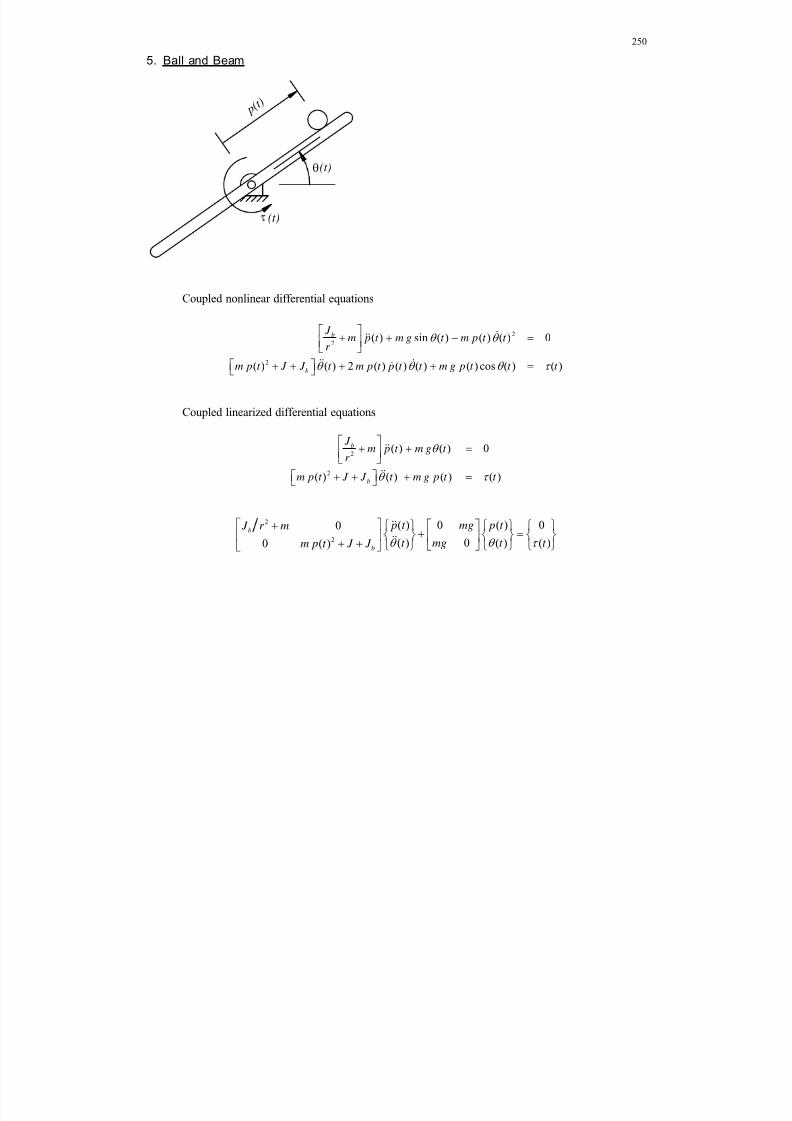
8/11/2019 Mechanism kinematics & dynamics.pdf
http://slidepdf.com/reader/full/mechanism-kinematics-dynamicspdf 250/269
250
5. Ball and Beam
Coupled nonlinear differential equations
2
2
2
( ) sin ( ) ( ) ( ) 0
( ) ( ) 2 ( ) ( ) ( ) ( ) cos ( ) ( )
b
b
J m p t m g t m p t t
r
m p t J J t m p t p t t m g p t t t
Coupled linearized differential equations
2
2
( ) ( ) 0
( ) ( ) ( ) ( )
b
b
J m p t m g t
r
m p t J J t m g p t t
2
2
( ) 0 ( ) 00
( ) 0 ( ) ( )0 ( )
b
b
p t mg p t J r m
t mg t t m p t J J
p ( t )
(t)
(t)
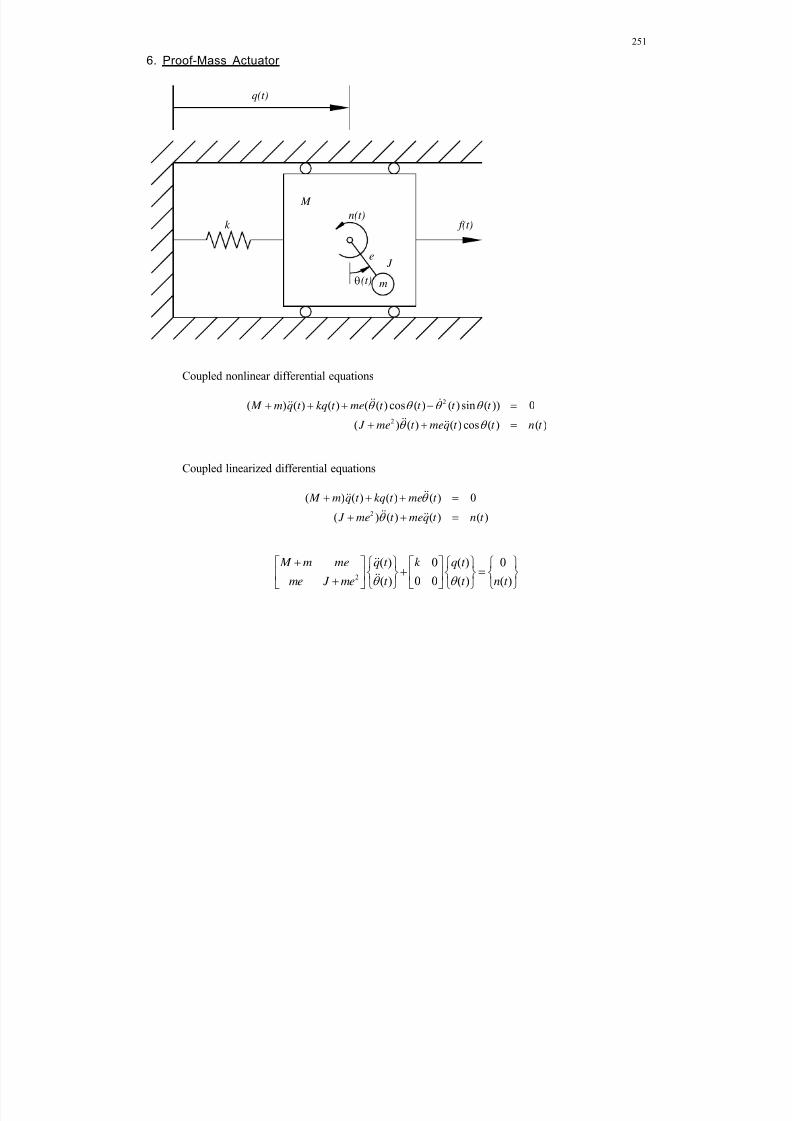
8/11/2019 Mechanism kinematics & dynamics.pdf
http://slidepdf.com/reader/full/mechanism-kinematics-dynamicspdf 251/269
251
6. Proof-Mass Actuator
Coupled nonlinear differential equations
2
2
( ) ( ) ( ) ( ( ) cos ( ) ( )sin ( )) 0
( ) ( ) ( ) cos ( ) ( )
M m q t kq t me t t t t
J me t meq t t n t
Coupled linearized differential equations
2
( ) ( ) ( ) ( ) 0
( ) ( ) ( ) ( )
M m q t kq t me t
J me t meq t n t
2
( ) 0 ( ) 0
( ) 0 0 ( ) ( )
M m me q t k q t
me J me t t n t
m
J
k
M
e
f(t)
q(t)
n(t)
(t)
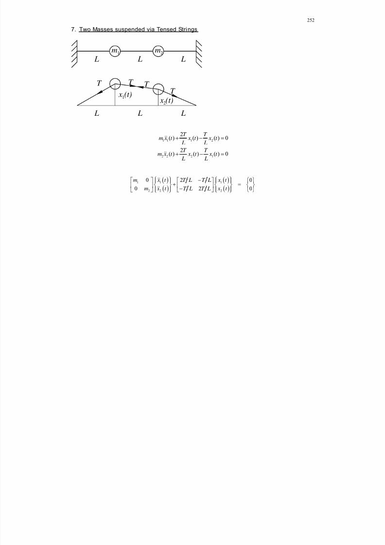
8/11/2019 Mechanism kinematics & dynamics.pdf
http://slidepdf.com/reader/full/mechanism-kinematics-dynamicspdf 252/269
252
7. Two Masses suspended via Tensed Strings
1 1 1 2
2 2 2 1
2( ) ( ) ( ) 0
2( ) ( ) ( ) 0
T T m x t x t x t
L L
T T m x t x t x t
L L
1 11
2 22
0 2 0
0 2 0
x t x t m T L T L
x t x t m T L T L
m L
x (t)
T T
1 m L
2
L
1 x (t)2
L L L
T T
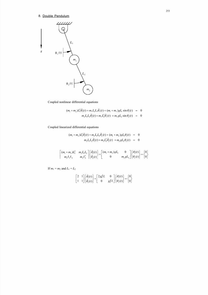
8/11/2019 Mechanism kinematics & dynamics.pdf
http://slidepdf.com/reader/full/mechanism-kinematics-dynamicspdf 253/269
253
8. Double Pendulum
Coupled nonlinear differential equations
2
1 2 1 1 2 1 2 2 1 2 1 1
2
2 1 2 1 2 2 2 2 2 2
( ) ( ) ( ) ( ) sin ( ) 0
( ) ( ) sin ( ) 0
m m L t m L L t m m gL t
m L L t m L t m gL t
Coupled linearized differential equations
2
1 2 1 1 2 1 2 2 1 2 1 1
2
2 1 2 1 2 2 2 2 2 2
( ) ( ) ( ) ( ) ( ) 0
( ) ( ) ( ) 0
m m L t m L L t m m gL t
m L L t m L t m gL t
21 2 1 11 2 1 2 1 2 1
22 2 22 1 2 2 2 2
( ) 0 ( ) 0( ) ( )
0 ( ) 0( )
m m gL t m m L m L L t
m gL t m L L m L t
If m1 = m2 and L1 = L2
11
22
( )2 1 2 0 0( )
( )1 1 0 0( )
t g Lt
t g Lt
L
1
1(t)
m1
L
2
2(t)
m2
g
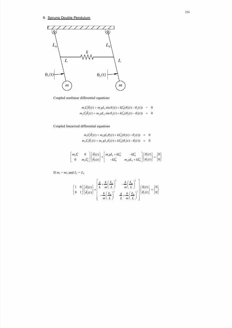
8/11/2019 Mechanism kinematics & dynamics.pdf
http://slidepdf.com/reader/full/mechanism-kinematics-dynamicspdf 254/269
254
9. Sprung Double Pendulum
Coupled nonlinear differential equations
2 2
1 1 1 1 1 1 0 1 2
2 2
2 2 2 2 2 2 0 2 1
( ) sin ( ) ( ( ) ( )) 0
( ) sin ( ) ( ( ) ( )) 0
m L t m gL t kL t t
m L t m gL t kL t t
Coupled linearized differential equations
2 2
1 1 1 1 1 1 0 1 2
2 2
2 2 2 2 2 2 0 2 1
( ) ( ) ( ( ) ( )) 0
( ) ( ) ( ( ) ( )) 0
m L t m gL t kL t t
m L t m gL t kL t t
2 2211 1 0 01 1 1
2 2220 2 2 02 2 2
( ) 00 ( )
( ) 00 ( )
t m gL kL kLm L t
t kL m gL kLm L t
If m1 = m2 and L1 = L2
2 2
0 0
11
2 222 0 0
( )1 0 0( )
( )0 1 0( )
L Lg k k
t L m L m Lt
t t L Lk g k
m L L m L
m
k
L
L0
m
L
(t)
L0
1 (t)2
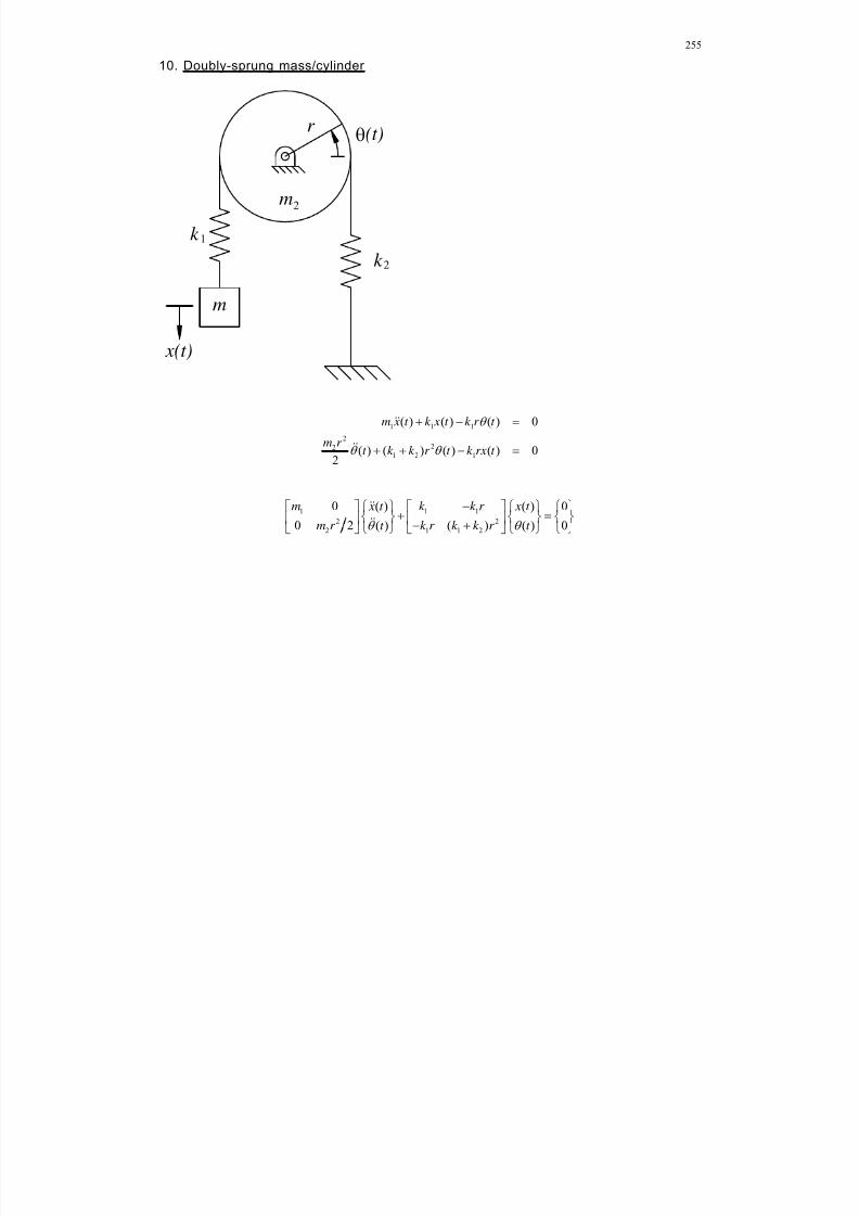
8/11/2019 Mechanism kinematics & dynamics.pdf
http://slidepdf.com/reader/full/mechanism-kinematics-dynamicspdf 255/269
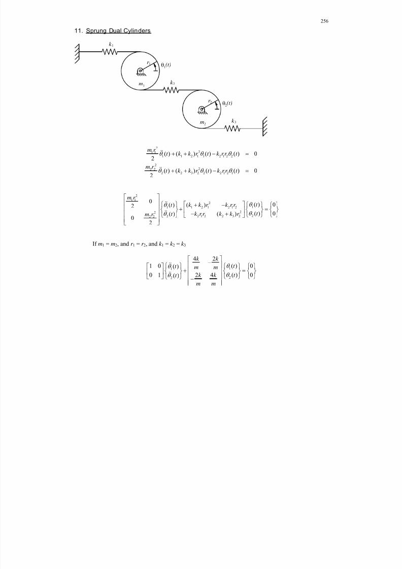
8/11/2019 Mechanism kinematics & dynamics.pdf
http://slidepdf.com/reader/full/mechanism-kinematics-dynamicspdf 256/269
256
11. Sprung Dual Cylinders
22
1 1 1 1 2 1 1 2 1 2 2
222 2
2 2 3 2 2 2 1 2 1
( ) ( ) ( ) ( ) 02
( ) ( ) ( ) ( ) 02
m r t k k r t k r r t
m r t k k r t k r r t
2
1 12
11 2 1 2 1 21
2222 1 2 2 3 222 2
0( ) 0( )( )2
( ) 0( )( )0
2
m r
t k k r k r r t
t k r r k k r t m r
If m1 = m2, and r 1 = r 2, and k 1 = k 2 = k 3
11
22
4 2
( )1 0 0( )
( )0 1 2 4 0( )
k k
t t m m
t k k t
m m
m k
r (t)
k m
r (t)
k

8/11/2019 Mechanism kinematics & dynamics.pdf
http://slidepdf.com/reader/full/mechanism-kinematics-dynamicspdf 257/269
257
12. Sprung Cart Pendulum
1 2 22
2 2 2
( ) ( ) ( ) 2 ( ) 0( ) ( ) ( ) 0
m m x t m L t kx t m L t m Lx t m Lg t
1 2 2
2
2 2 2
2 0( ) ( ) 0
0( ) ( ) 0
m m m L k x t x t
m L m L m Lgt t
m
k x(t)
(t)
k
1
m2

8/11/2019 Mechanism kinematics & dynamics.pdf
http://slidepdf.com/reader/full/mechanism-kinematics-dynamicspdf 258/269
258
13. Translating rotating rigid body
This is a 2-dof system, still constrained to vibrate in the vertical direction, with small-anglerotational vibrations as well.
1 2 1 1 2 2
2 2
1 1 2 2 1 1 2 2
( ) ( ) ( ) ( ) ( ) 0
( ) ( ) ( ) ( ) ( ) 0
mx t k k x t k L k L t
J t k L k L x t k L k L t
1 2 1 1 2 2
2 2
1 1 2 2 1 1 2 2
0 ( ) ( ) 0
0 ( ) ( ) 0
k k k L k Lm x t x t
k L k L k L k L J t t
m, J
k
(t)
k 1 2
x(t)
L L1 2
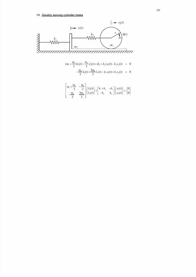
8/11/2019 Mechanism kinematics & dynamics.pdf
http://slidepdf.com/reader/full/mechanism-kinematics-dynamicspdf 259/269
259
14. Doubly sprung cylinder mass
2 21 1 2 1 2 1 2 2
2 21 2 2 1 2 2
( ) ( ) ( ) ( ) ( ) ( ) 02 2
3( ) ( ) ( ) ( ) 0
2 2
m mm x t x t k k x t k x t
m m x t x t k x t k x t
2 21
1 1 2 2 1
2 2 2 22 2
( ) ( ) 02 2
( ) ( )3 0
2 2
m mm
x t k k k x t
x t k k x t m m
m
k
x (t)
r (t)2
2
k 1
m1
2
x (t)1
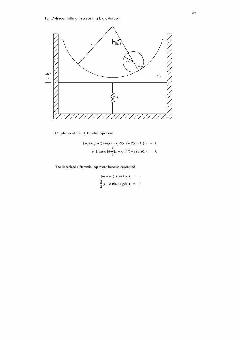
8/11/2019 Mechanism kinematics & dynamics.pdf
http://slidepdf.com/reader/full/mechanism-kinematics-dynamicspdf 260/269
260
15. Cylinder rolling in a sprung big cylinder
Coupled nonlinear differential equations
1 2 2 1 2
1 2
( ) ( ) ( ) ( )sin ( ) ( ) 0
3( )sin ( ) ( ) ( ) sin ( ) 0
2
m m x t m r r t t kx t
x t t r r t g t
The linearized differential equations become decoupled.
1 2
1 2
( ) ( ) ( ) 0
3( ) ( ) ( ) 02
m m x t kx t
r r t g t
m
r
(t)
2
2
r 1
k
m1 x(t)
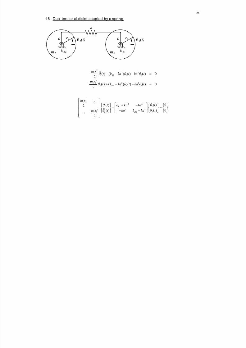
8/11/2019 Mechanism kinematics & dynamics.pdf
http://slidepdf.com/reader/full/mechanism-kinematics-dynamicspdf 261/269
261
16. Dual torsional disks coupled by a spring
22 21 1
1 1 1 2
22 22 2
2 2 2 1
( ) ( ) ( ) ( ) 02
( ) ( ) ( ) ( ) 02
R
R
m r t k ka t ka t
m r t k ka t ka t
2
1 12 2
111
2 222222 2
0( ) 0( )2
( ) 0( )0
2
R
R
m r
t k ka kat
t ka k kat m r
m
k
r (t)a1
1
k R11m
r (t)a2
2
k R22

8/11/2019 Mechanism kinematics & dynamics.pdf
http://slidepdf.com/reader/full/mechanism-kinematics-dynamicspdf 262/269
262
17. Dual point masses
1 1 1 2 1 2 2
2 2 2 2 2 2 1
( ) ( ) ( ) 2 ( ) ( )
( ) ( ) 4 ( ) 2 ( ) 0
m x t k k x t k x t f t
m x t cx t k x t k x t
1 1 1 1 2 2 1
2 2 2 2 2 2
0 ( ) ( ) 2 ( )0 0 ( )
0 ( ) ( ) 2 4 ( )0 0
m x t x t k k k x t f t
m x t x t k k x t c
k c
m
x (t)
1k 2
1m2
L L
1 x (t)
2
f(t)

8/11/2019 Mechanism kinematics & dynamics.pdf
http://slidepdf.com/reader/full/mechanism-kinematics-dynamicspdf 263/269
263
18. Rotating sprung point masses
2 2
( ) 2 ( ) ( ) 0
2 ( ) 2 ( ) ( ) ( )
mx t kx t kL t
mL t kL t kLx t t
2 2
0 ( ) 2 ( ) 0
0 2 ( ) 2 ( ) ( )
m x t k kL x t
mL t kL kL t t
k
m
x(t)
L L
k
mm
k
(t)
(t)

8/11/2019 Mechanism kinematics & dynamics.pdf
http://slidepdf.com/reader/full/mechanism-kinematics-dynamicspdf 264/269
264
19. Three-Mass Vibrational System
1 1 1 2 1 1 2 1 2 2 2 2 1
2 2 2 3 2 2 3 2 2 1 2 1 3 3 3 3 2
3 3 3 4 3 3 4 3 3 2 3 2 3
( ) ( ) ( ) ( ) ( ) ( ) ( ) ( )
( ) ( ) ( ) ( ) ( ) ( ) ( ) ( ) ( ) ( )
( ) ( ) ( ) ( ) ( ) ( ) ( ) ( )
m y t c c y t k k y t c y t k y t u t
m y t c c y t k k y t c y t k y t c y t k y t u t
m y t c c y t k k y t c y t k y t u t
1 1 1 2 2 1 1 2 2 1 1
2 2 2 2 3 3 2 2 2 3 3 2 2
3 3 3 3 4 3 3 3 4 3 3
0 0 ( ) 0 ( ) 0 ( ) ( )
0 0 ( ) ( ) ( ) ( )
0 0 ( ) 0 ( ) 0 ( ) (
m y t c c c y t k k k y t u t
m y t c c c c y t k k k k y t u t
m y t c c c y t k k k y t u
)t
y (t)
m1 m2 m3
k 1 k 2 k 3
c1 c2 c3
k 4
c4
1 y (t)
2 y (t)
3
u (t)1
u (t)2
u (t)3
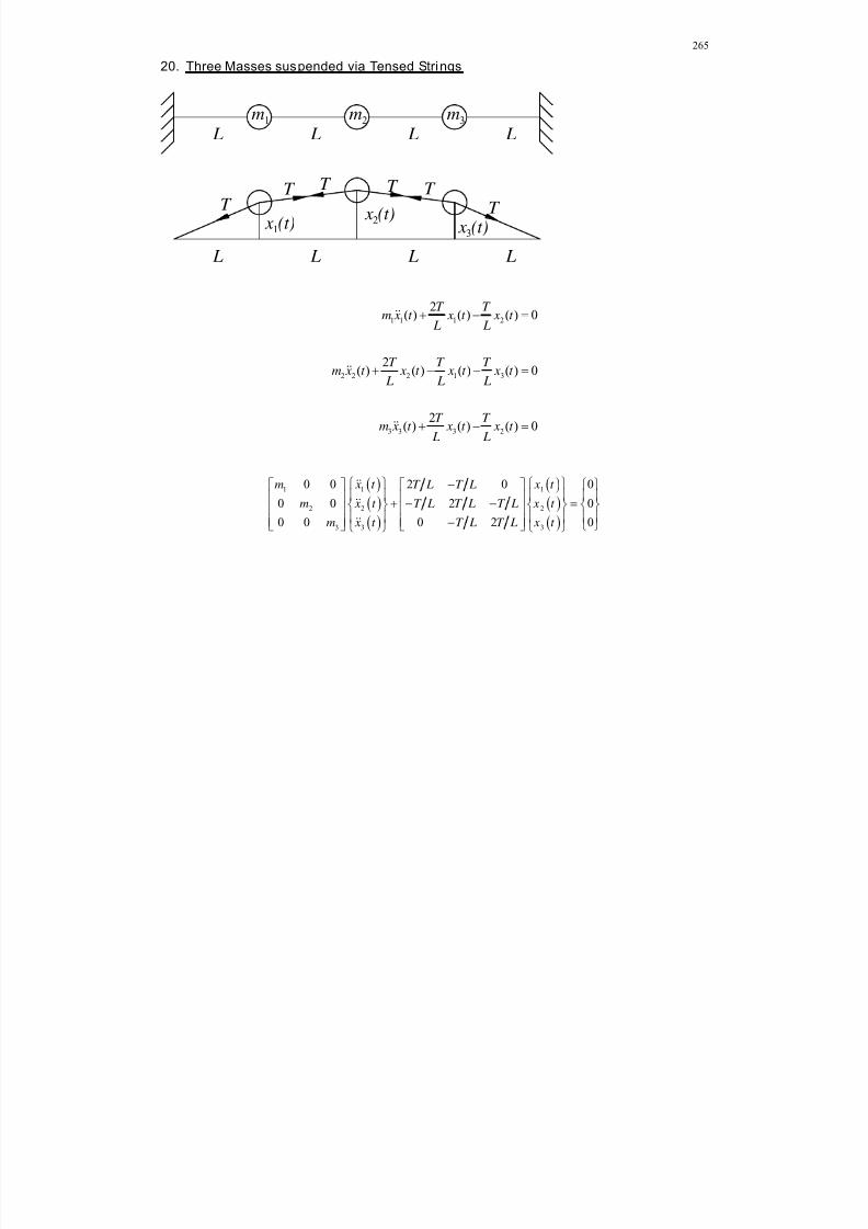
8/11/2019 Mechanism kinematics & dynamics.pdf
http://slidepdf.com/reader/full/mechanism-kinematics-dynamicspdf 265/269
265
20. Three Masses suspended via Tensed Strings
1 1 1 2
2 2 2 1 3
3 3 3 2
2( ) ( ) ( ) 0
2( ) ( ) ( ) ( ) 0
2( ) ( ) ( ) 0
T T m x t x t x t
L L
T T T m x t x t x t x t
L L L
T T m x t x t x t
L L
1 1 1
2 2 2
3 3 3
0 0 2 0 0
0 0 2 0
0 0 0 2 0
m x t T L T L x t
m x t T L T L T L x t
m x t T L T L x t
m L
x (t)
T T
1 m L
2
L
2 x (t)3
L L L
m3
L
T T
T T
L
x (t)1
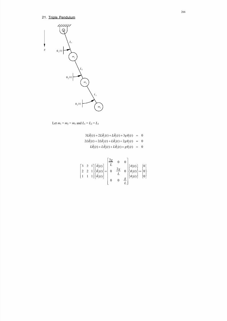
8/11/2019 Mechanism kinematics & dynamics.pdf
http://slidepdf.com/reader/full/mechanism-kinematics-dynamicspdf 266/269
266
21. Triple Pendulum
Let m1 = m2 = m3 and L1 = L2 = L3
1 2 3 1
1 2 3 2
1 2 3 3
3 ( ) 2 ( ) ( ) 3 ( ) 0
2 ( ) 2 ( ) ( ) 2 ( ) 0
( ) ( ) ( ) ( ) 0
L t L t L t g t
L t L t L t g t
L t L t L t g t
1 1
2 2
3 3
30 0
3 2 1 ( ) ( ) 02
2 2 1 ( ) 0 0 ( ) 0
1 1 1 ( ) ( ) 0
0 0
g
Lt t g
t t
Lt t g
L
L
1
1(t)
m1
L
2
2(t)
m2
L
3
3(t)
m3
g
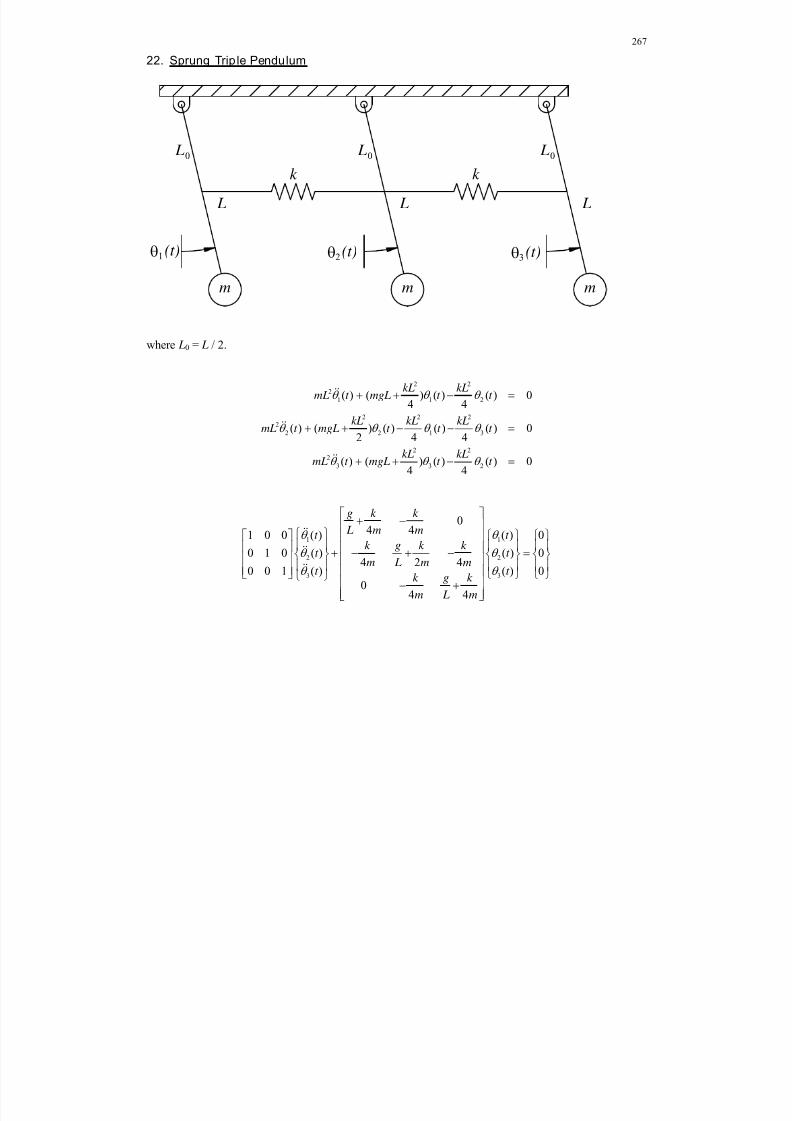
8/11/2019 Mechanism kinematics & dynamics.pdf
http://slidepdf.com/reader/full/mechanism-kinematics-dynamicspdf 267/269
267
22. Sprung Trip le Pendulum
where L0 = L / 2.
2 22
1 1 2
2 2 22
2 2 1 3
2 22
3 3 2
( ) ( ) ( ) ( ) 04 4
( ) ( ) ( ) ( ) ( ) 02 4 4
( ) ( ) ( ) ( ) 04 4
kL kLmL t mgL t t
kL kL kLmL t mgL t t t
kL kLmL t mgL t t
1 1
2 2
3 3
04 41 0 0 ( ) ( ) 0
0 1 0 ( ) ( ) 04 2 4
0 0 1 ( ) ( ) 0
04 4
g k k
L m mt t k g k k
t t m L m m
t t k g k
m L m
m
k
L
L0
m
L
(t)
L0
m
k
L
L0
1 (t)2 (t)3
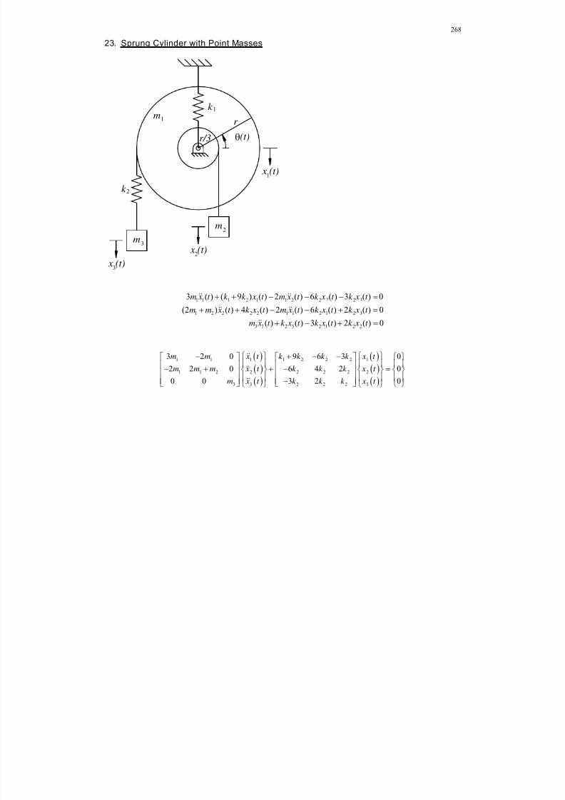
8/11/2019 Mechanism kinematics & dynamics.pdf
http://slidepdf.com/reader/full/mechanism-kinematics-dynamicspdf 268/269
268
23. Sprung Cylinder with Point Masses
1 1 1 2 1 1 2 2 2 2 3
1 2 2 2 2 1 1 2 1 2 3
3 3 2 3 2 1 2 2
3 ( ) ( 9 ) ( ) 2 ( ) 6 ( ) 3 ( ) 0
(2 ) ( ) 4 ( ) 2 ( ) 6 ( ) 2 ( ) 0
( ) ( ) 3 ( ) 2 ( ) 0
m x t k k x t m x t k x t k x t
m m x t k x t m x t k x t k x t
m x t k x t k x t k x t
1 1 1 1 2 2 2 1
1 1 2 2 2 2 2 2
3 3 2 2 2 3
3 2 0 9 6 3 0
2 2 0 6 4 2 0
0 0 3 2 0
m m x t k k k k x t
m m m x t k k k x t
m x t k k k x t
m
m
k
x (t)
r
(t)
k
r/3
m
x (t)
x (t)
8/11/2019 Mechanism kinematics & dynamics.pdf
http://slidepdf.com/reader/full/mechanism-kinematics-dynamicspdf 269/269
269
Common Model Features
Considering all multi-dof vibrational models we have derived, some general comments can bemade about the models.


