Mechanics
Cartesian Coordinates
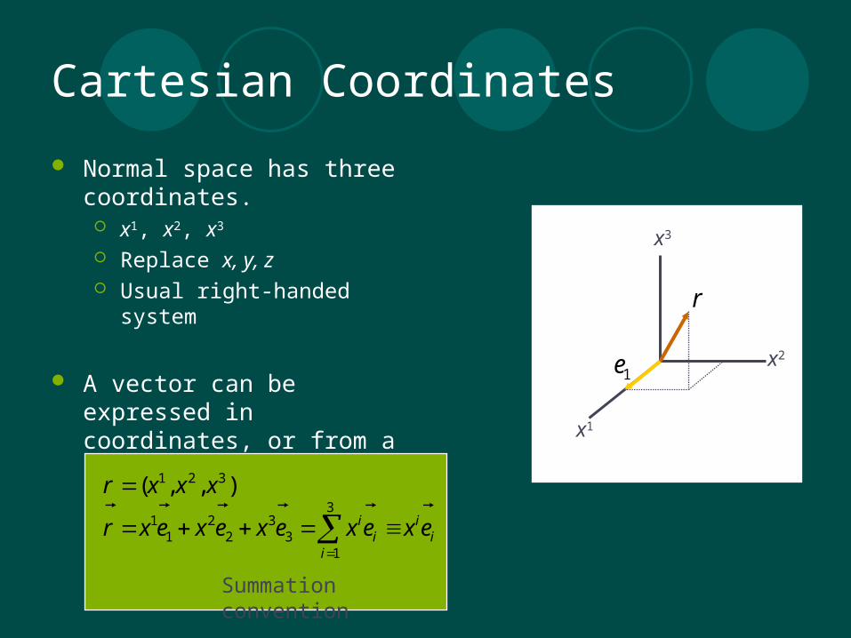
Normal space has three coordinates.
x1, x2, x3
Replace x, y, z Usual right-handed system
A vector can be expressed in coordinates, or from a basis.
Unit vectors form a basis x1
x2
x3
1e
ii
ii
i exexexexexr
3
13
32
21
1
),,( 321 xxxr
Summation convention
r
Cartesian Algebra
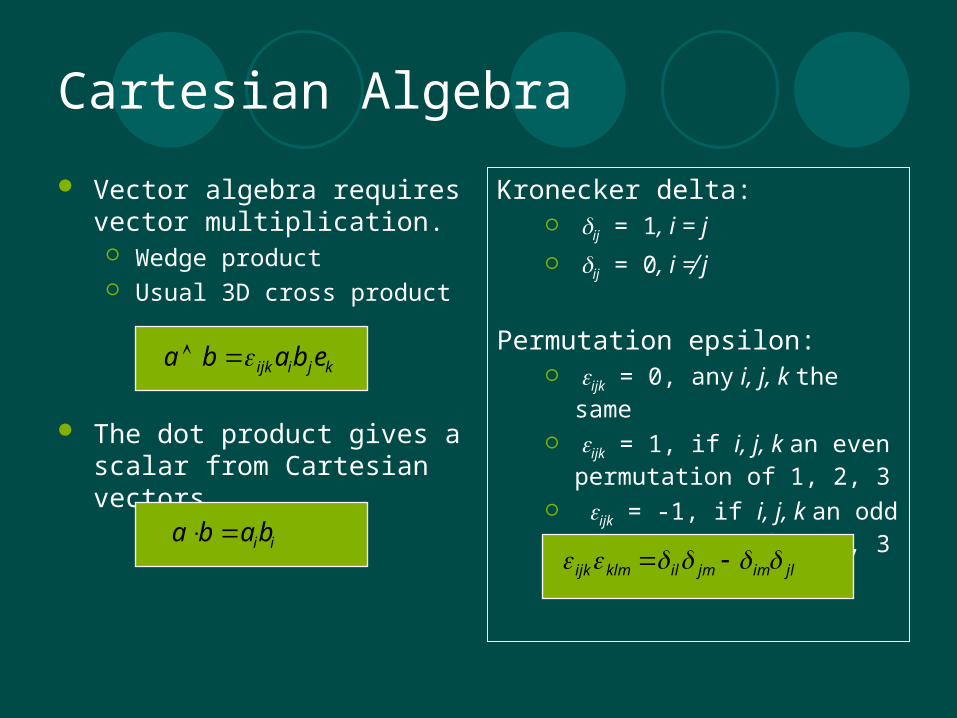
Vector algebra requires vector multiplication.
Wedge product Usual 3D cross product
The dot product gives a scalar from Cartesian vectors.
Kronecker delta: ij = 1, i = j
ij = 0, i ≠ j
Permutation epsilon: ijk = 0, any i, j, k the same
ijk = 1, if i, j, k an even permutation of 1, 2, 3
ijk = -1, if i, j, k an odd permutation of 1, 2, 3
kjiijk ebaba
jlimjmilklmijk iibaba
Coordinate Transformation
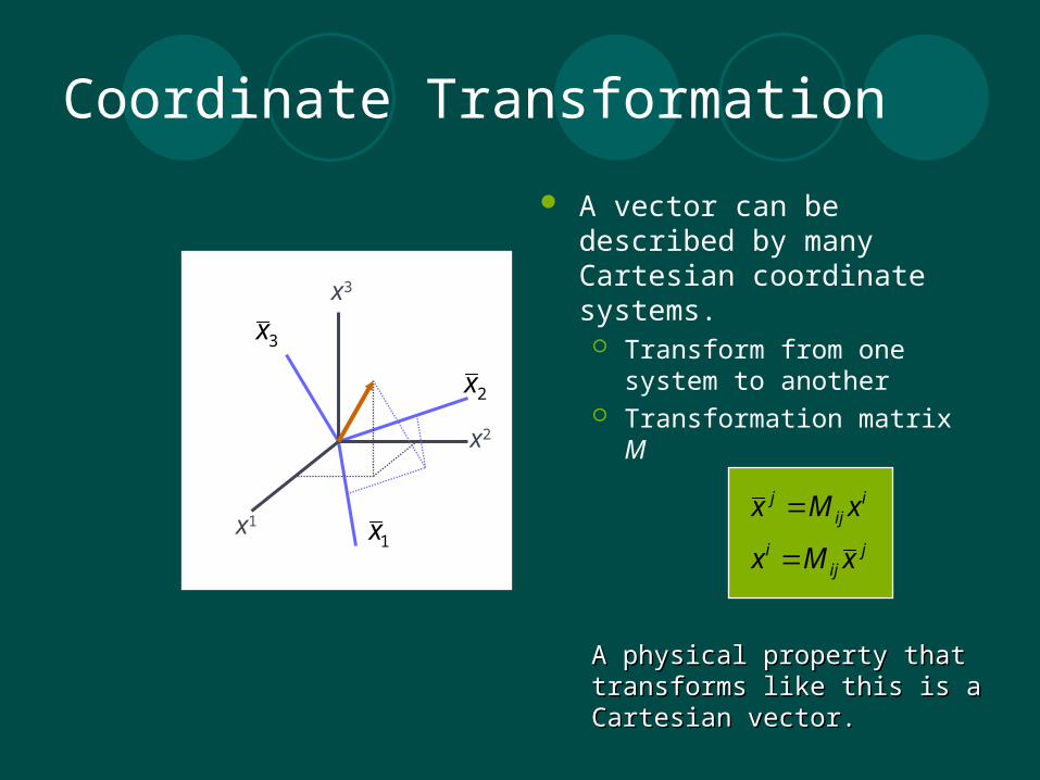
A vector can be described by many Cartesian coordinate systems.
Transform from one system to another
Transformation matrix M
x1
x2
x3
jij
i xMx
iij
j xMx 1x
2x
3x
A physical property that transforms A physical property that transforms like this is a Cartesian vector.like this is a Cartesian vector.
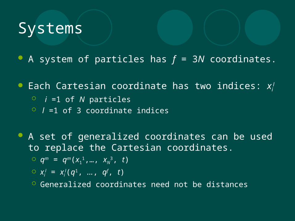
Systems
A system of particles has f = 3N coordinates.
Each Cartesian coordinate has two indices: xil
i =1 of N particles l =1 of 3 coordinate indices
A set of generalized coordinates can be used to replace the Cartesian coordinates. qm = qm(x1
1,…, xN3, t)
xil = xi
l(q1, …, qf, t) Generalized coordinates need not be distances
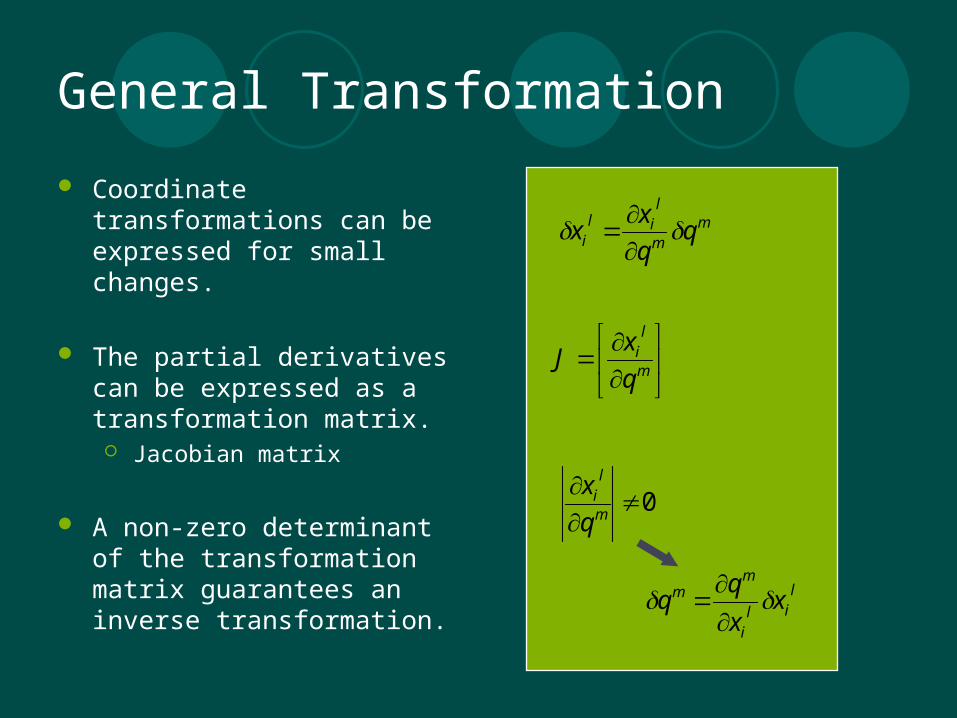
General Transformation
Coordinate transformations can be expressed for small changes.
The partial derivatives can be expressed as a transformation matrix.
Jacobian matrix
A non-zero determinant of the transformation matrix guarantees an inverse transformation.
mm
lil
i qq
xx
lil
i
mm x
x
0
m
li
q
x
m
li
q
xJ
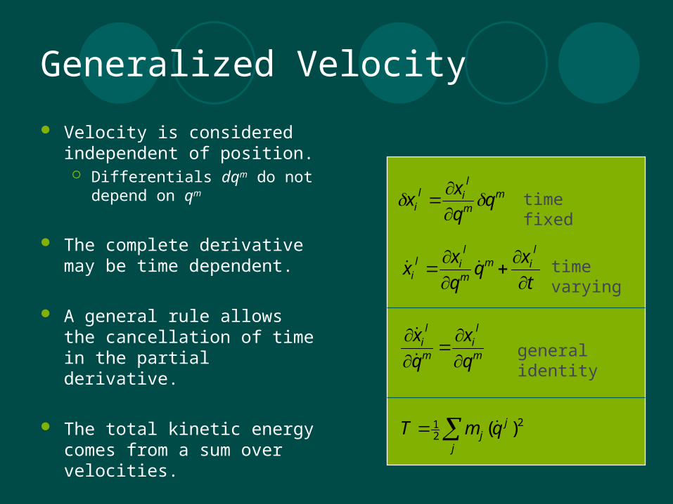
Generalized Velocity
Velocity is considered independent of position.
Differentials dqm do not depend on qm
The complete derivative may be time dependent.
A general rule allows the cancellation of time in the partial derivative.
The total kinetic energy comes from a sum over velocities.
t
xq
q
xx
lim
m
lil
i
mm
lil
i qq
xx
m
li
m
li
q
x
q
x
time fixed
time varying
general identity
j
jj qmT 2
21 )(
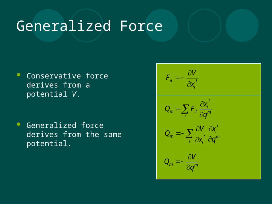
Generalized Force
Conservative force derives from a potential V.
Generalized force derives from the same potential.
i
m
li
li
m q
x
x
VQ
li
ilx
VF
i
m
li
ilm q
xFQ
mm q
VQ
Lagrangian
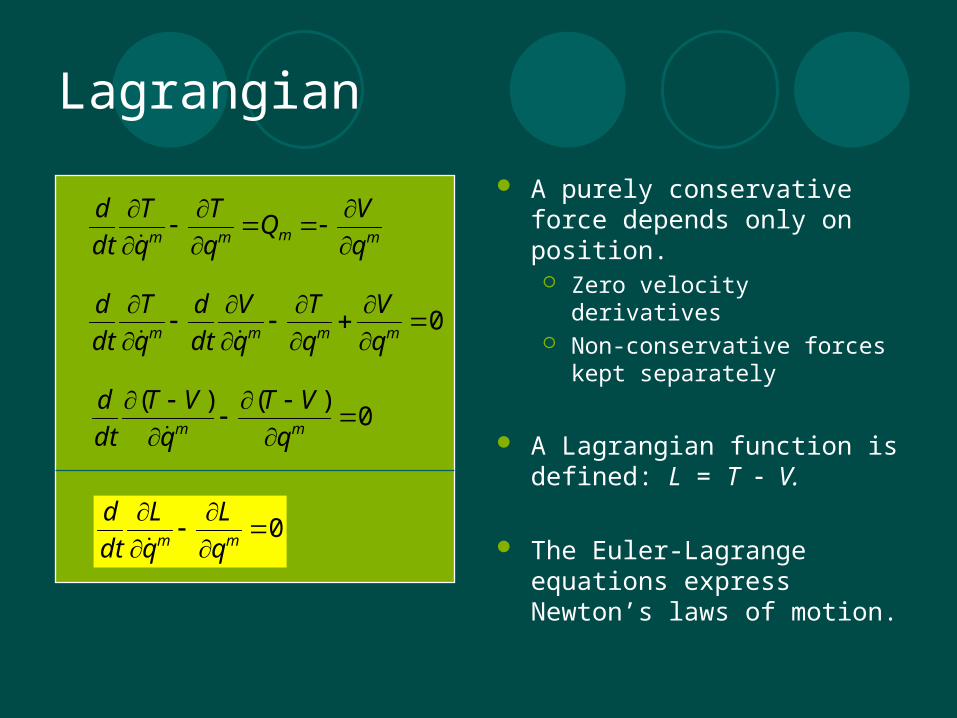
A purely conservative force depends only on position.
Zero velocity derivatives Non-conservative forces kept
separately
A Lagrangian function is defined: L = T V.
The Euler-Lagrange equations express Newton’s laws of motion.
mmmm q
VQ
q
T
q
T
dt
d
0
mmmm q
V
q
T
q
V
dt
d
q
T
dt
d
0)()(
mm q
VT
q
VT
dt
d
0
mm q
L
q
L
dt
d
Generalized Momentum
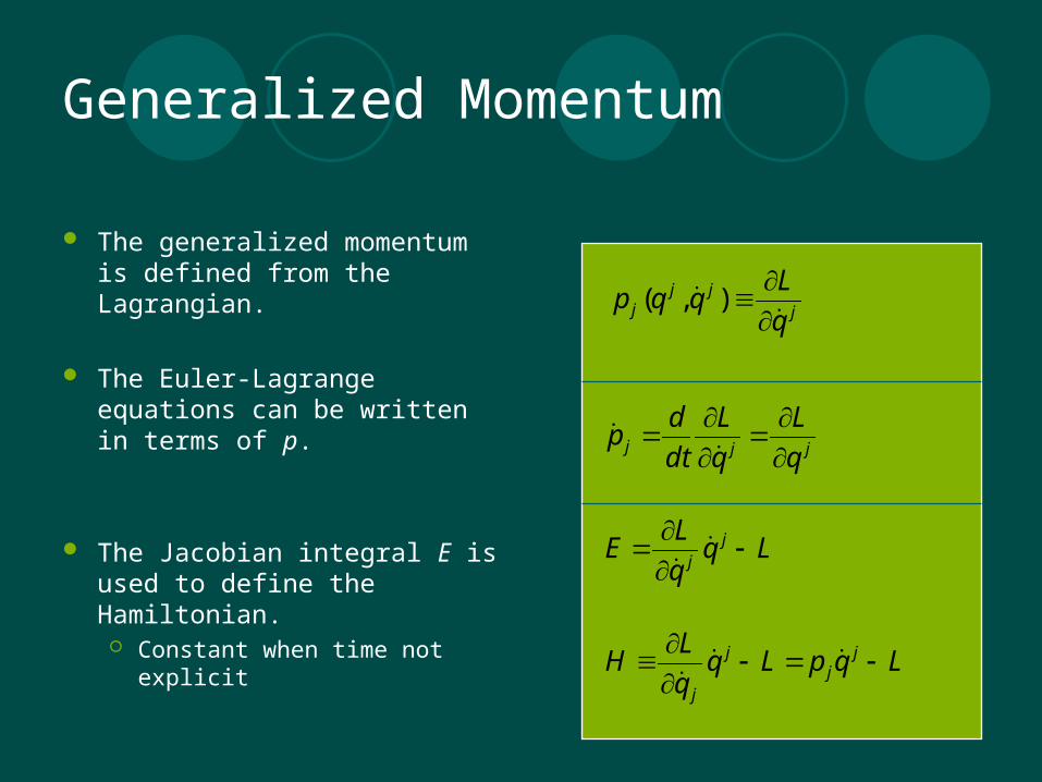
The generalized momentum is defined from the Lagrangian.
The Euler-Lagrange equations can be written in terms of p.
The Jacobian integral E is used to define the Hamiltonian.
Constant when time not explicit
jjj
j q
Lqqp
),(
jjj q
L
q
L
dt
dp
Lqq
LE j
j
LqpLqq
LH j
jj
j
Canonical Equations
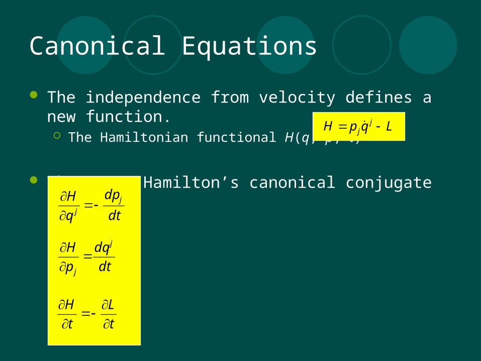
The independence from velocity defines a new function. The Hamiltonian functional H(q, p, t)
These are Hamilton’s canonical conjugate equations.
dt
dq
p
H j
j
dt
dp
q
H j
j
t
L
t
H
LqpH jj
Space Trajectory
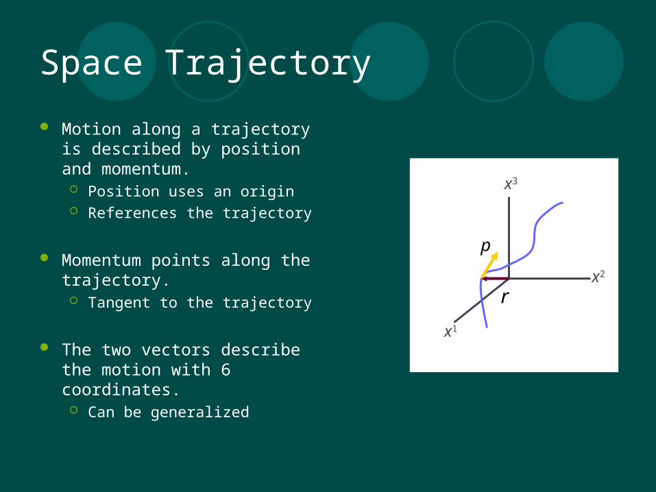
Motion along a trajectory is described by position and momentum.
Position uses an origin References the trajectory
Momentum points along the trajectory.
Tangent to the trajectory
The two vectors describe the motion with 6 coordinates.
Can be generalized
x1
x2
x3
p
r
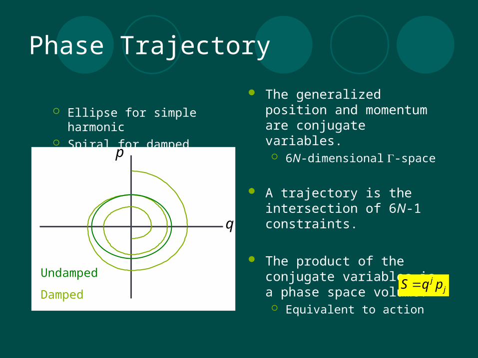
Phase Trajectory
Ellipse for simple harmonic Spiral for damped harmonic
q
p
Undamped
Damped
The generalized position and momentum are conjugate variables.
6N-dimensional -space
A trajectory is the intersection of 6N-1 constraints.
The product of the conjugate variables is a phase space volume.
Equivalent to action jj pqS
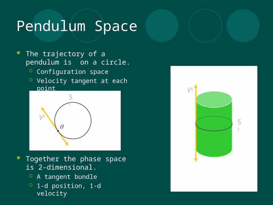
Pendulum Space
The trajectory of a pendulum is on a circle.
Configuration space Velocity tangent at each point
Together the phase space is 2-dimensional.
A tangent bundle 1-d position, 1-d velocity
V1
S1
V1
S1
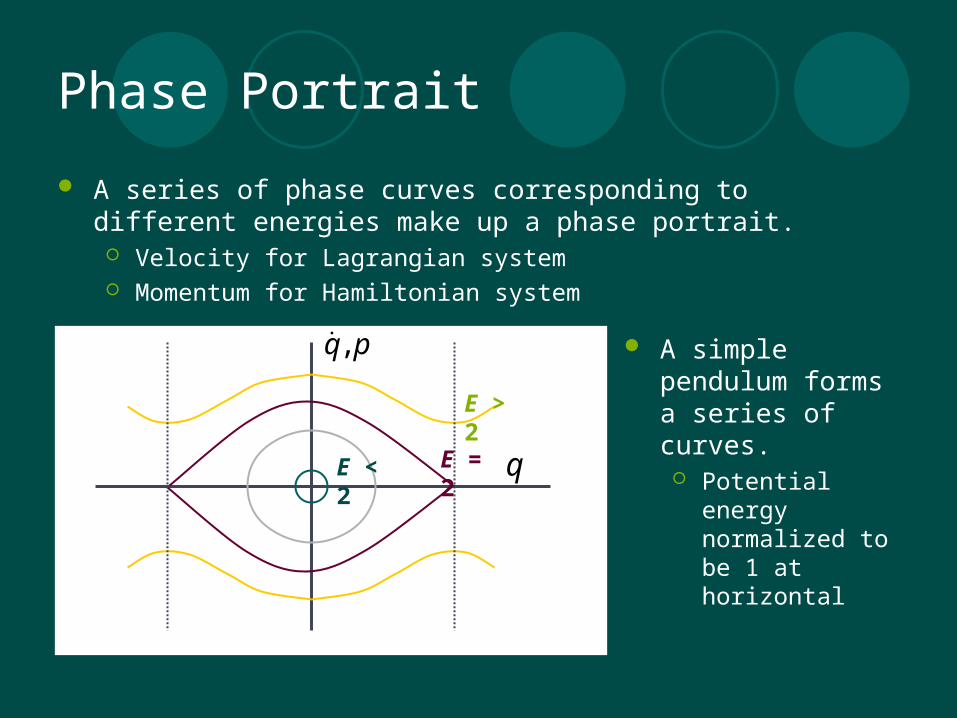
Phase Portrait
A series of phase curves corresponding to different energies make up a phase portrait.
Velocity for Lagrangian system Momentum for Hamiltonian system
q
pq,
E < 2 E = 2
E > 2
A simple pendulum forms a series of curves.
Potential energy normalized to be 1 at horizontal
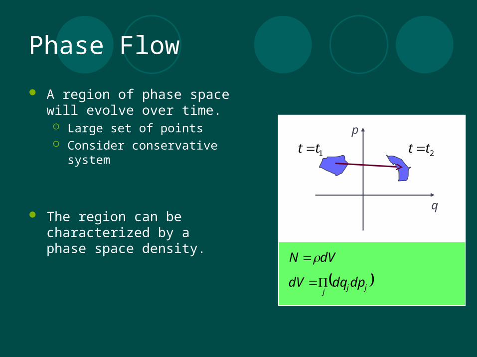
Phase Flow
A region of phase space will evolve over time.
Large set of points Consider conservative system
The region can be characterized by a phase space density.
dVN
2tt 1tt
q
p
jjj
dpdqdV
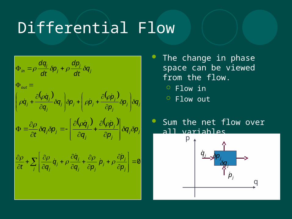
Differential Flow
jj
jj
in qdt
dpp
dt
dq
jj
j
j
j
jjj pq
p
p
q
qpq
t
The change in phase space can be viewed from the flow.
Flow in Flow out
Sum the net flow over all variables.
jj
j
jjjj
j
jj
out
qpp
pppq
q
0
j j
jj
jj
jj
j p
pp
pq
qt
q
p
jq
jp
jpjq
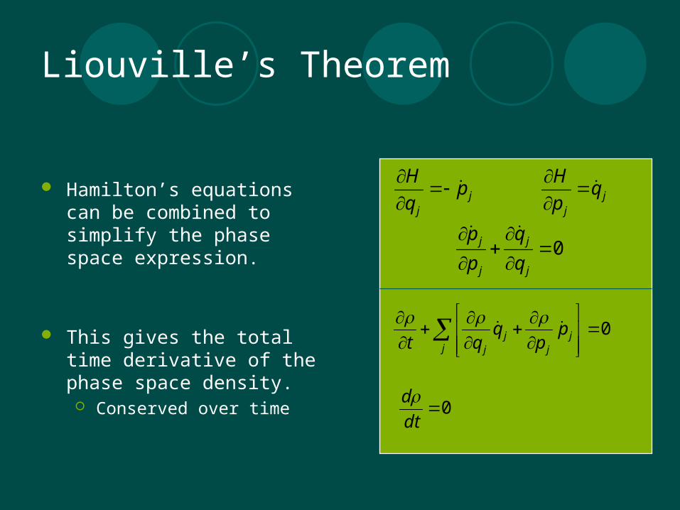
Liouville’s Theorem
Hamilton’s equations can be combined to simplify the phase space expression.
This gives the total time derivative of the phase space density.
Conserved over time
jj
pq
H
jj
qp
H
0
j
j
j
j
q
q
p
p
0
jj
jj
j
pp
qqt
0dt
d
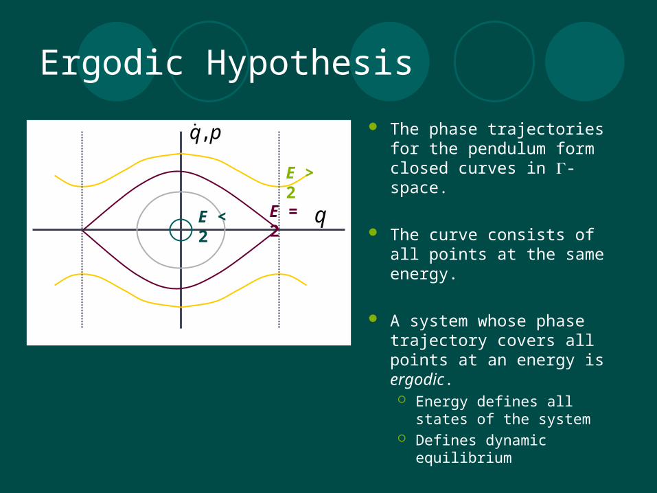
Ergodic Hypothesis
The phase trajectories for the pendulum form closed curves in -space.
The curve consists of all points at the same energy.
A system whose phase trajectory covers all points at an energy is ergodic.
Energy defines all states of the system
Defines dynamic equilibrium
q
pq,
E < 2 E = 2
E > 2
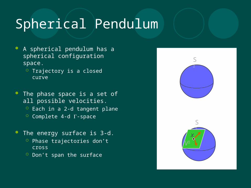
Spherical Pendulum
A spherical pendulum has a spherical configuration space.
Trajectory is a closed curve
The phase space is a set of all possible velocities.
Each in a 2-d tangent plane Complete 4-d -space
The energy surface is 3-d. Phase trajectories don’t cross Don’t span the surface
S2
xV2
S2
Non-Ergodic Systems
The spherical pendulum is non-ergodic. A phase trajectory does not reach all energy points
Two-dimensional harmonic oscillator with commensurate periods is non-ergodic.
Many simple systems in multiple dimensions are non-ergodic. Energy is insufficient to define all states of a system.
Quasi-Ergodic Hypothesis
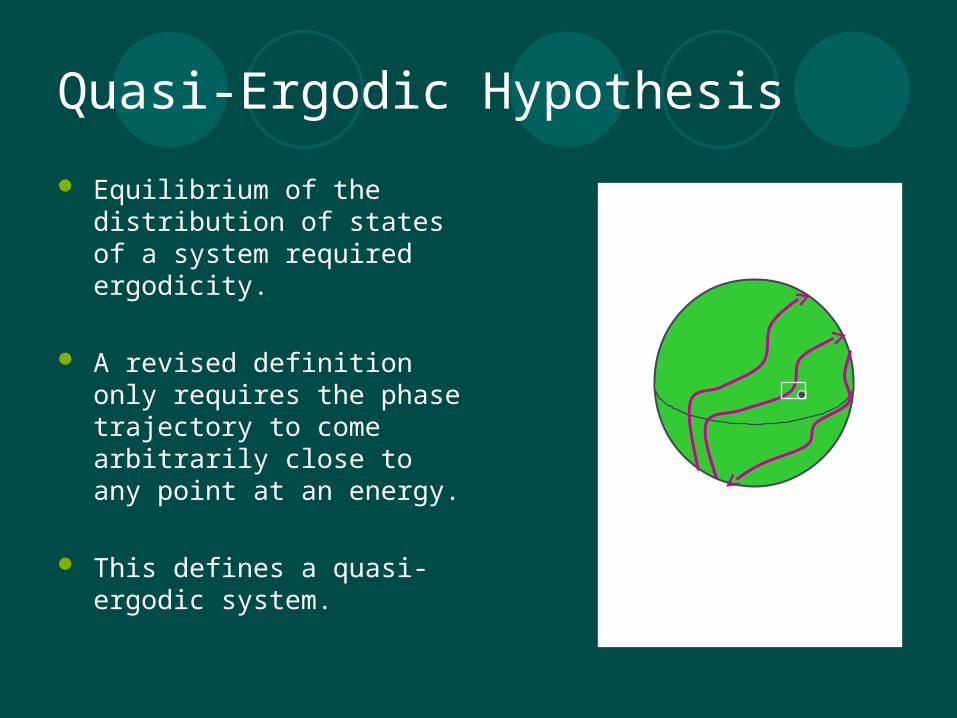
Equilibrium of the distribution of states of a system required ergodicity.
A revised definition only requires the phase trajectory to come arbitrarily close to any point at an energy.
This defines a quasi-ergodic system.
Quasi-Ergodic Definition
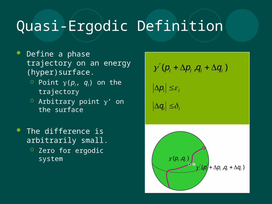
Define a phase trajectory on an energy (hyper)surface.
Point (pi, qi) on the trajectory Arbitrary point ’ on the
surface
The difference is arbitrarily small.
Zero for ergodic system
iip
),( iiii qqpp
iiq
),( iiii qqpp ),( ii qp
Coarse Grain
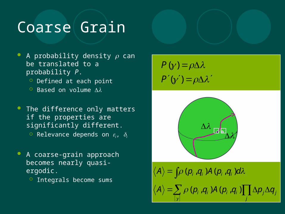
A probability density can be translated to a probability P.
Defined at each point Based on volume
The difference only matters if the properties are significantly different.
Relevance depends on i, i
A coarse-grain approach becomes nearly quasi-ergodic.
Integrals become sums
)(P
jjjiiii qpqpAqpA
),(),(
)(P
dqpAqpA iiii ),(),(


