
Mechanical Geometry Theorem Proving
Automated ReasoningThursday 15th Nov. 2007
Laura I. Meikle
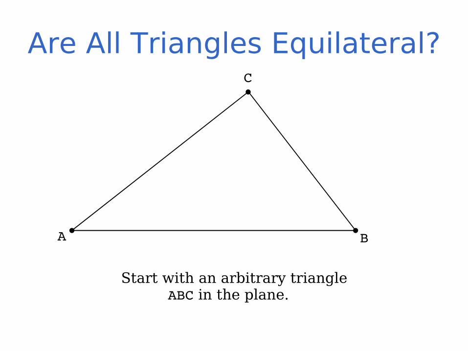
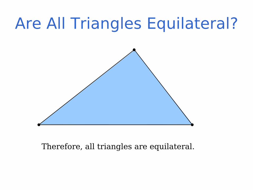
Are All Triangles Equilateral?
BA
Start with an arbitrary triangleABC in the plane.
C
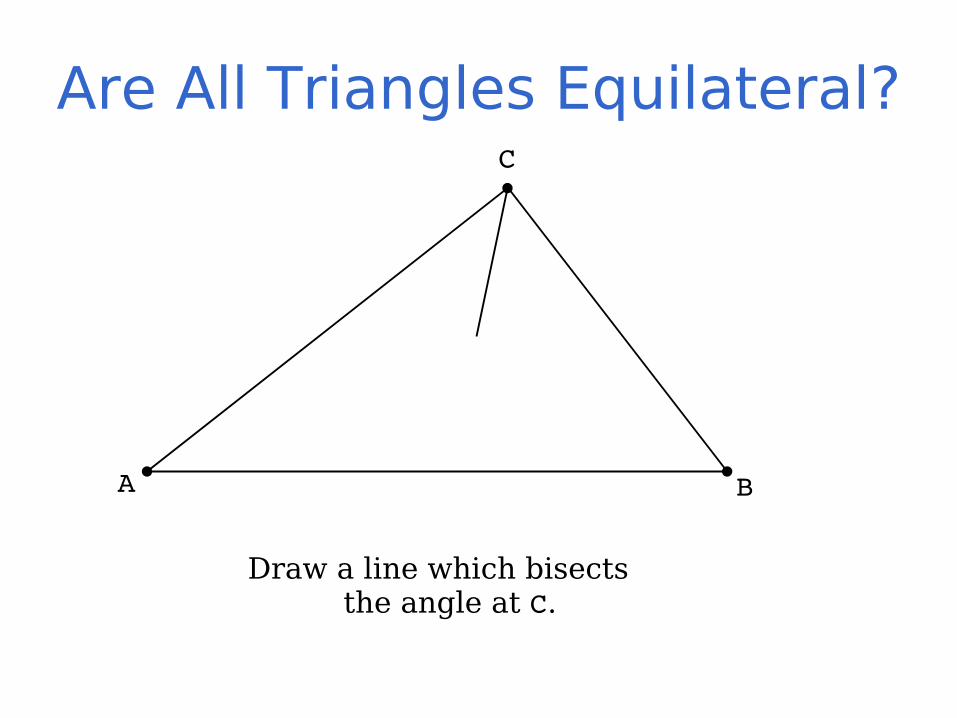
Are All Triangles Equilateral?C
BA
Draw a line which bisectsthe angle at C.
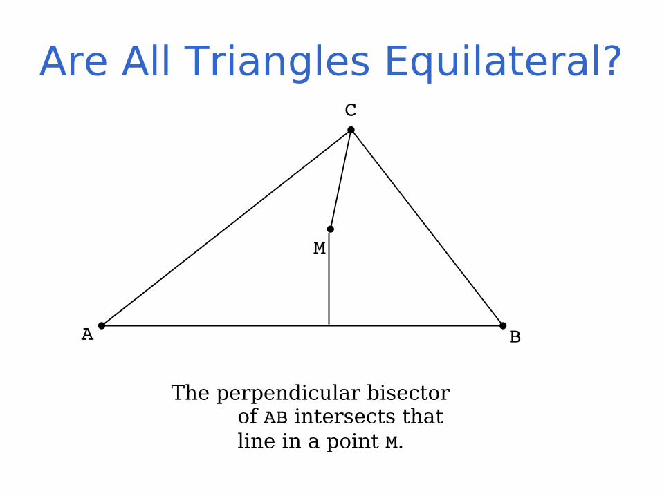
Are All Triangles Equilateral?C
M
BA
The perpendicular bisectorof AB intersects thatline in a point M.

Are All Triangles Equilateral?C
M
BA
Draw from the intersection M the normal lines to the
other two sides.

Are All Triangles Equilateral?C
M
R Q
P BA
Finally, connect the point M to A and M to B.
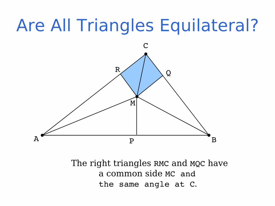
Are All Triangles Equilateral?C
R Q
P BA
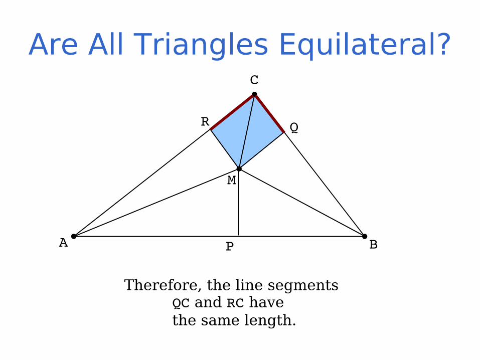
The right triangles RMC and MQC havea common side MC andthe same angle at C.
M
Are All Triangles Equilateral?C
R Q
P BA
Therefore, the line segmentsQC and RC havethe same length.
M
Are All Triangles Equilateral?C
R Q
P BA
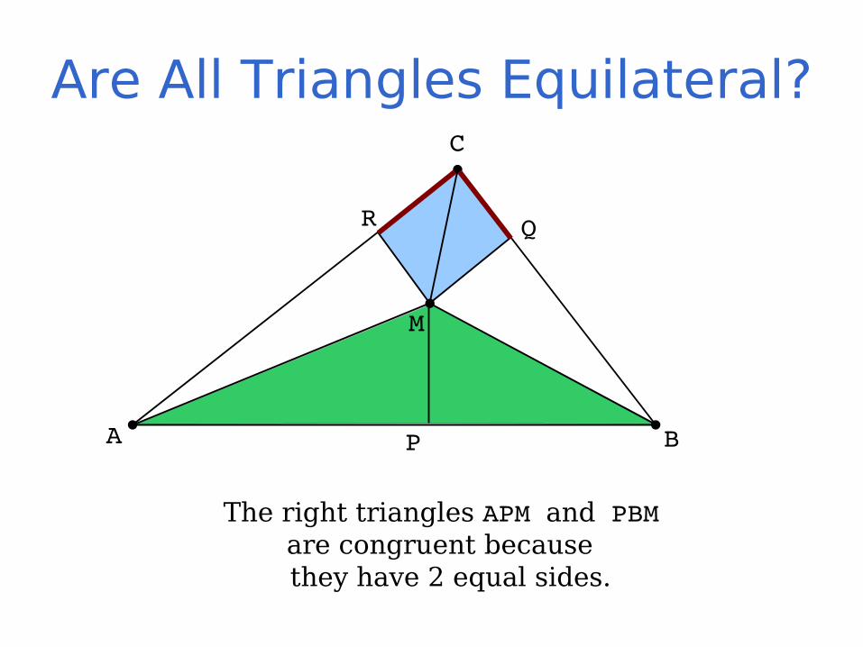
The right triangles APM and PBM are congruent because they have 2 equal sides.
M

Are All Triangles Equilateral?C
R Q
P BA
Therefore the segments AM and BMare the same length.
M
Are All Triangles Equilateral?C
R Q
P BA
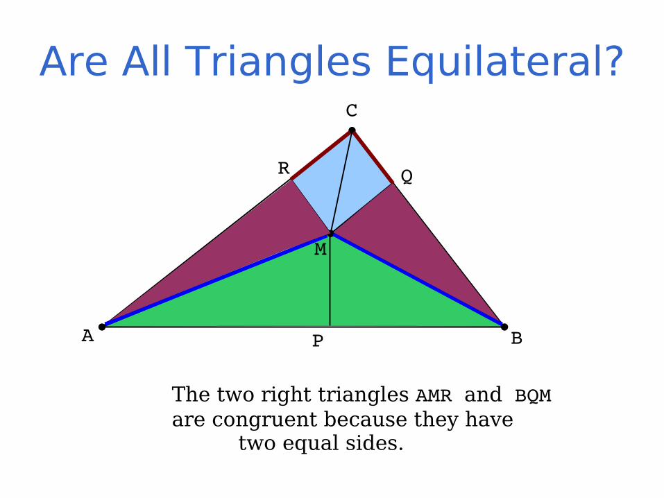
The two right triangles AMR and BQM are congruent because they have
two equal sides.
M

Are All Triangles Equilateral?C
R Q
P BA
Therefore the segments AR and BQ
have equal length.
M
Are All Triangles Equilateral?C
R Q
P BA
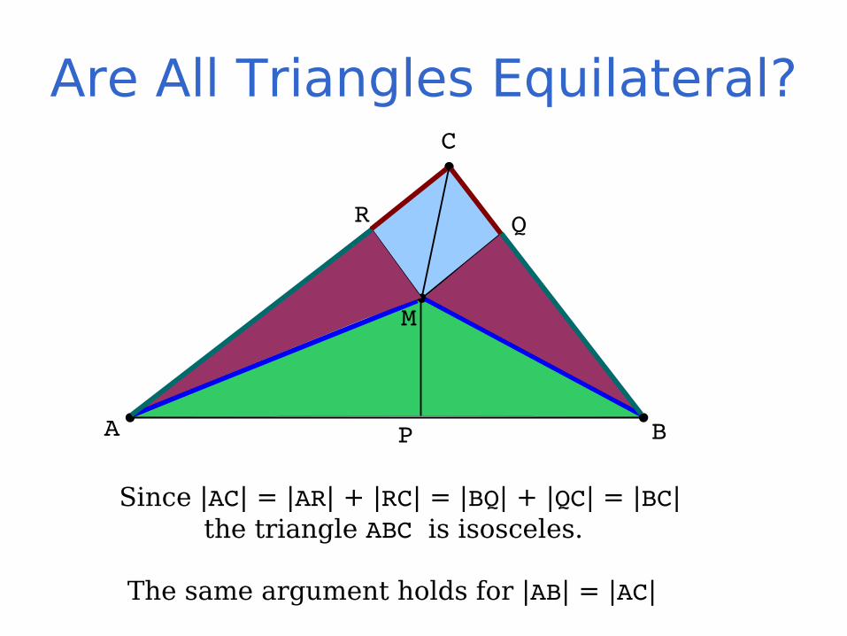
Since |AC| = |AR| + |RC| = |BQ| + |QC| = |BC| the triangle ABC is isosceles.
The same argument holds for |AB| = |AC|
M
Are All Triangles Equilateral?
Therefore, all triangles are equilateral.

What is a Proof?
• Diagrams can be a minefield for mistakes
• So what is a proof?
– One which is accepted by community?– Human intuition needed?– Completely logical?
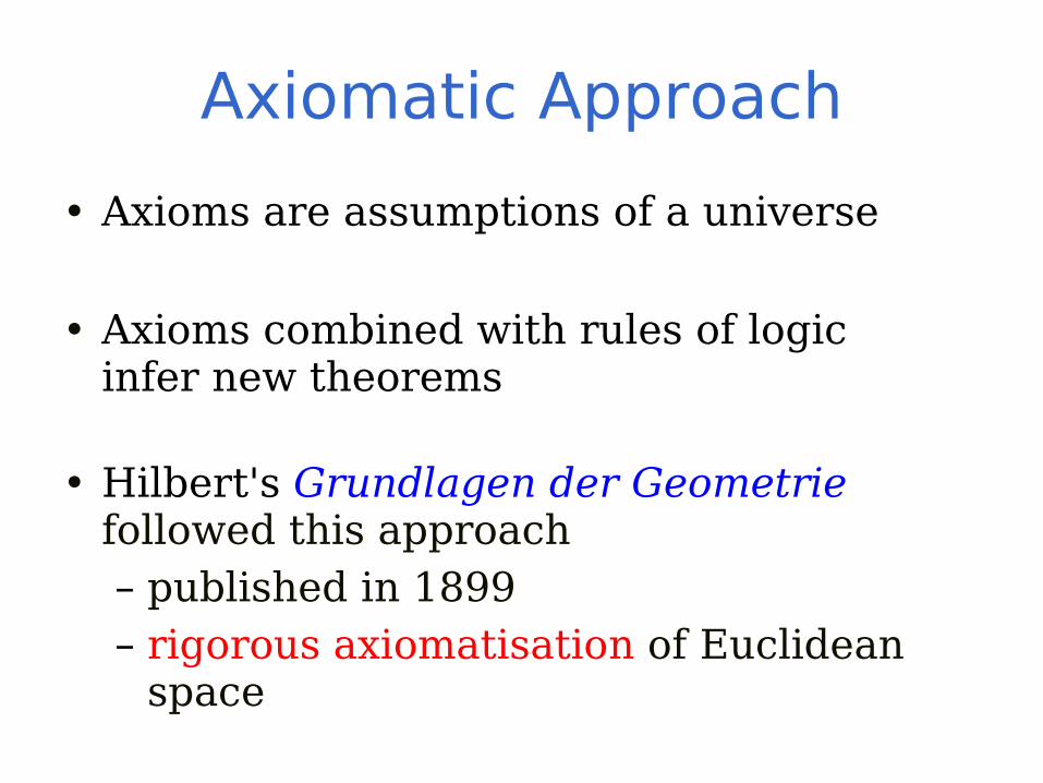
Axiomatic Approach
• Axioms are assumptions of a universe
• Axioms combined with rules of logicinfer new theorems
• Hilbert's Grundlagen der Geometrie followed this approach– published in 1899– rigorous axiomatisation of Euclidean
space

Hilbert's Grundlagen• 3 primitive objects: points, lines, planes
– Claim: it is not necessary to assign any explicit meaning to these primitives
– They could be chairs, tables and beer mugs!
• Relationships between the primitives described and categorised into 5 groups of axioms– Using primitive relations: on line, between, ...
– Axioms minimal and complete
– Ex: for every two points A, B there exists a line a that contains each of the points A, B.
Hilbert claimed his proofs were free of intuition and required only his axioms and the rules of logic
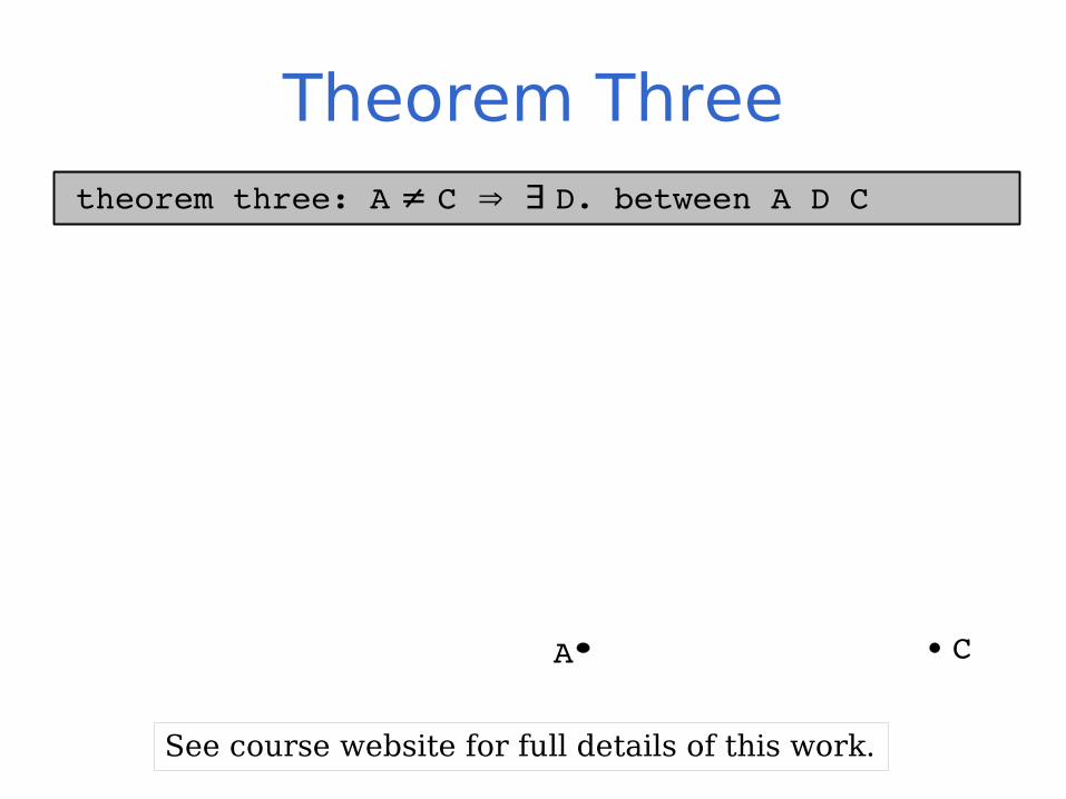
Theorem Three theorem three: A ≠ C ∃ D. between A D C
CA
See course website for full details of this work.

Theorem Three
Grundlagen Proof:
By Axiom (I,3) thereexists a point E outside the line AC.
AxI3: A B C. A ∃ ≠ B ∧ A ≠ C ∧ B ≠ C ∧ ¬coll{A,B,C}
C
E
AMissing:Need to construct a linethat A and C lie on.
theorem three: A ≠ C ∃ D. between A D C
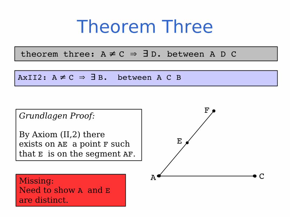
Theorem Three
Grundlagen Proof:
By Axiom (II,2) thereexists on AE a point F such that E is on the segment AF.
AxII2: A ≠ C ∃ B. between A C B
C
E
A
F
Missing:Need to show A and E are distinct.
theorem three: A ≠ C ∃ D. between A D C
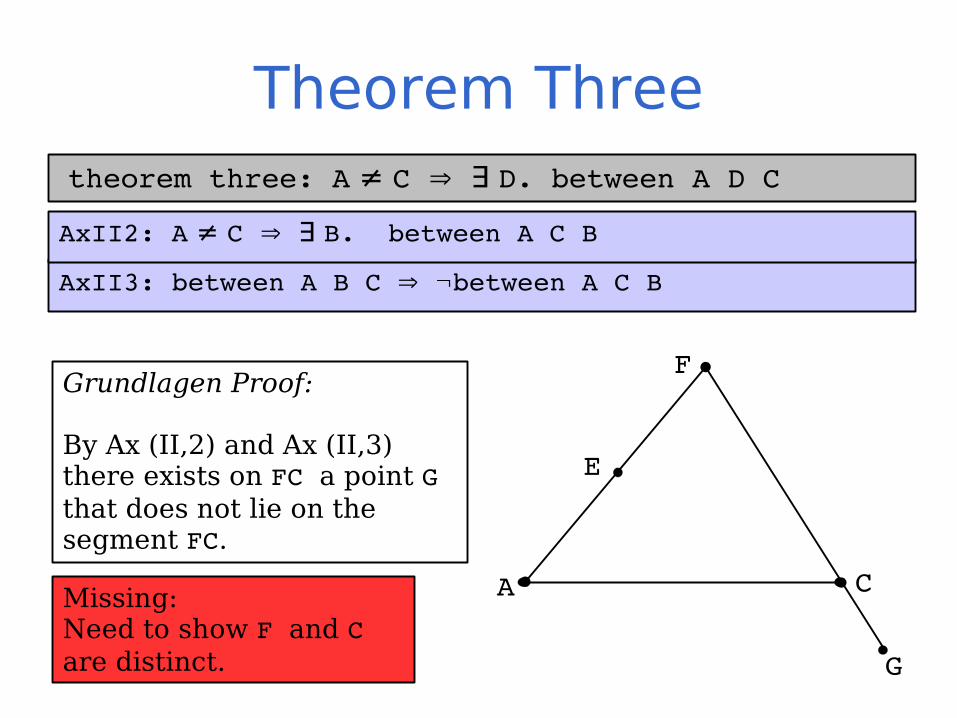
Theorem Three
Grundlagen Proof:
By Ax (II,2) and Ax (II,3) there exists on FC a point G that does not lie on the segment FC.
AxII3: between A B C ¬between A C B
Missing:Need to show F and C are distinct.
C
E
A
F
G
AxII2: A ≠ C ∃ B. between A C B
theorem three: A ≠ C ∃ D. between A D C
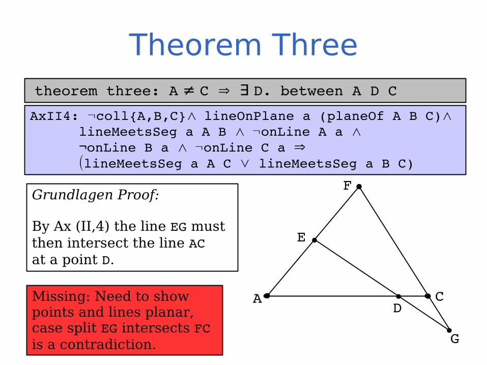
Theorem Three
Grundlagen Proof:
By Ax (II,4) the line EG mustthen intersect the line ACat a point D.
Missing: Need to show points and lines planar, case split EG intersects FC is a contradiction.
C
E
A
F
G
AxII4: ¬coll{A,B,C}∧ lineOnPlane a (planeOf A B C)∧lineMeetsSeg a A B ∧ ¬onLine A a ∧ ¬onLine B a ∧ ¬onLine C a (lineMeetsSeg a A C ∨ lineMeetsSeg a B C)
D
theorem three: A ≠ C ∃ D. between A D C
Observations
• Hilbert made implicit assumptions
– newly constructed points were distinct– the existence of specific lines (i.e. AC)
– all points and lines were planar– case split omitted
• Diagram appeals to our intuition
• Diagram could be reason for missing steps in proof
Story So Far ...
• Proving geometric results is challenging:
– Diagrams can be misleading– Even Hilbert relied on intuition
• Confidence in geometric results suspect?• Formal computerised proof would give
reassurances– especially needed when results relied
upon for safety-critical applications

CG
Databases Computer graphics
Computer vision
Air Traffic Control
Statistics
Robotics
Molecular biology
Manufacturing
Computational Geometry
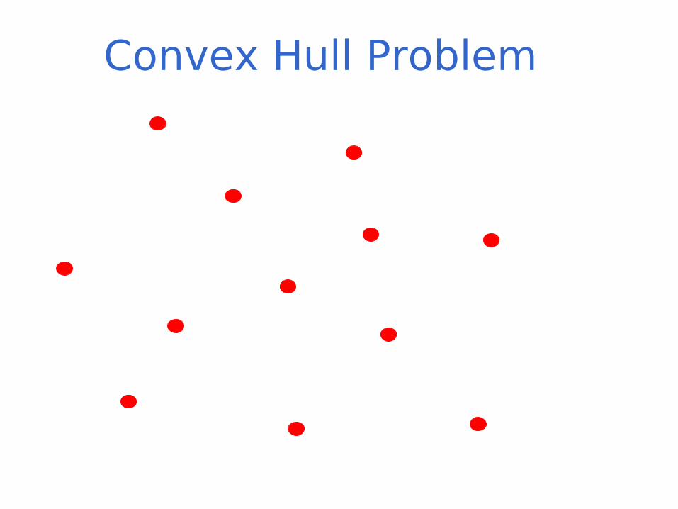
Convex Hull Problem

Convex Hull Problem
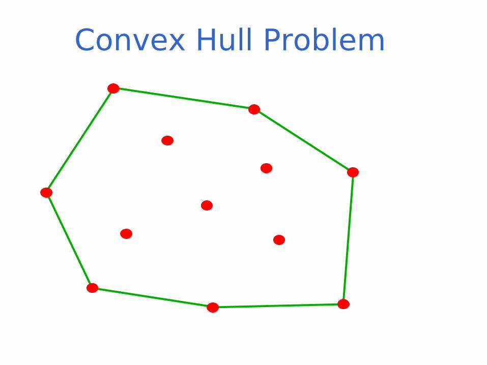
Convex Hull Problem
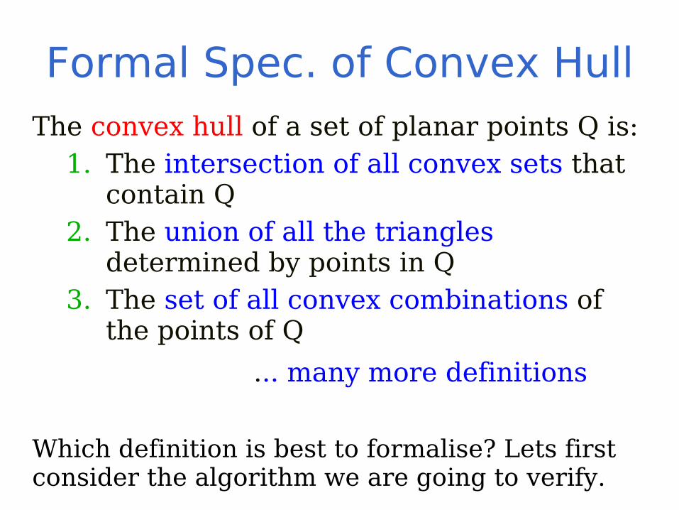
Formal Spec. of Convex HullThe convex hull of a set of planar points Q is:
1. The intersection of all convex sets that contain Q
2. The union of all the triangles determined by points in Q
3. The set of all convex combinations of the points of Q
... many more definitions
Which definition is best to formalise? Lets first consider the algorithm we are going to verify.
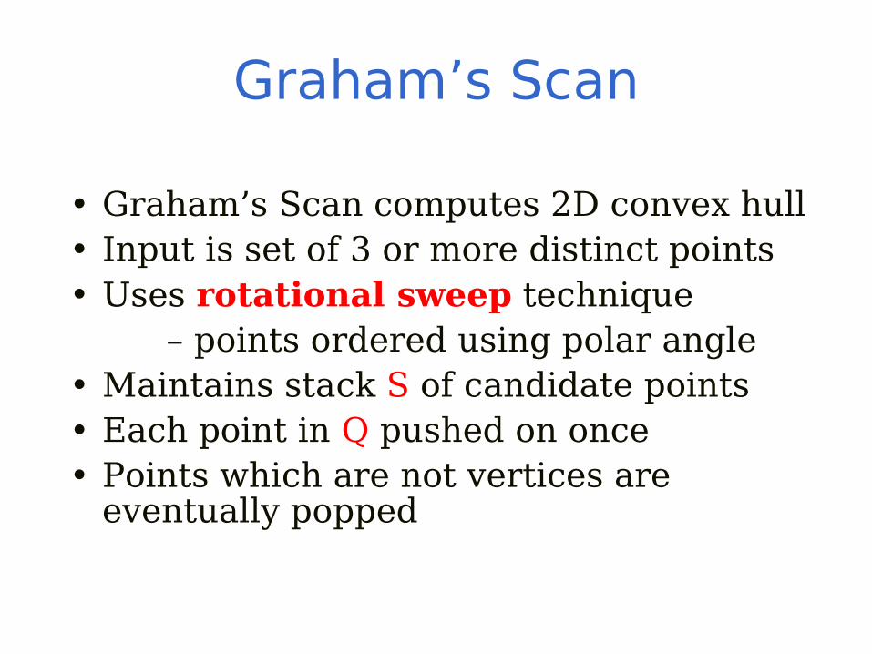
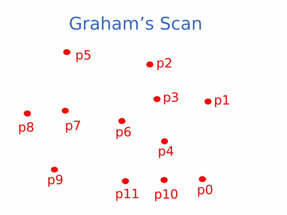
Graham’s Scan
• Graham’s Scan computes 2D convex hull• Input is set of 3 or more distinct points• Uses rotational sweep technique – points ordered using polar angle• Maintains stack S of candidate points• Each point in Q pushed on once• Points which are not vertices are
eventually popped

Graham’s Scan
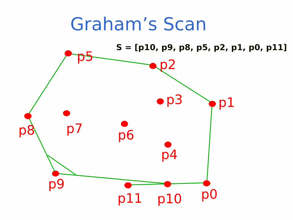
Find rightmost lowest point; label it p0. Sort all other points angularly about p0, break ties in favour of closeness to p0; label p1, …, pn1 Stack S=(pn1,p0)=(pt1,pt); t indexes top. i = 1 while i < n do if pi is strictly left of (pt1,pt) then Push(S,pi) and set i i + 1→ else Pop(S)
p7
Graham’s Scan
p0
p1
p2
p3
p4
p5
p6p8
p9p10p11

p7
Graham’s Scan
p0
p1
p2
p3
p4
p5
p6p8
p9p10p11
S = [p1, p0, p11]

p7
Graham’s Scan
p0
p1
p2
p3
p4
p5
p6p8
p9p10p11
S = [p2, p1, p0, p11]
p7
Graham’s Scan
p0
p1
p2
p3
p4
p5
p6p8
p9p10p11
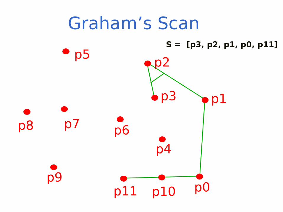
S = [p3, p2, p1, p0, p11]
p7
Graham’s Scan
p0
p1
p2
p3
p4
p5
p6p8
p9p10p11
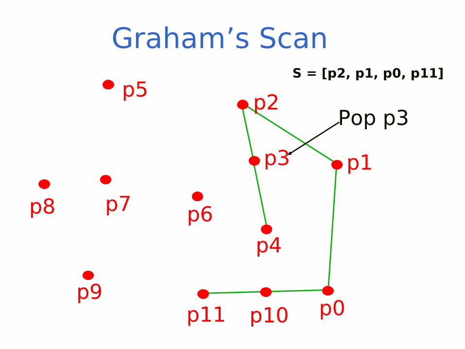
Pop p3
S = [p2, p1, p0, p11]
p7
Graham’s Scan
p0
p1
p2
p3
p4
p5
p6p8
p9p10p11
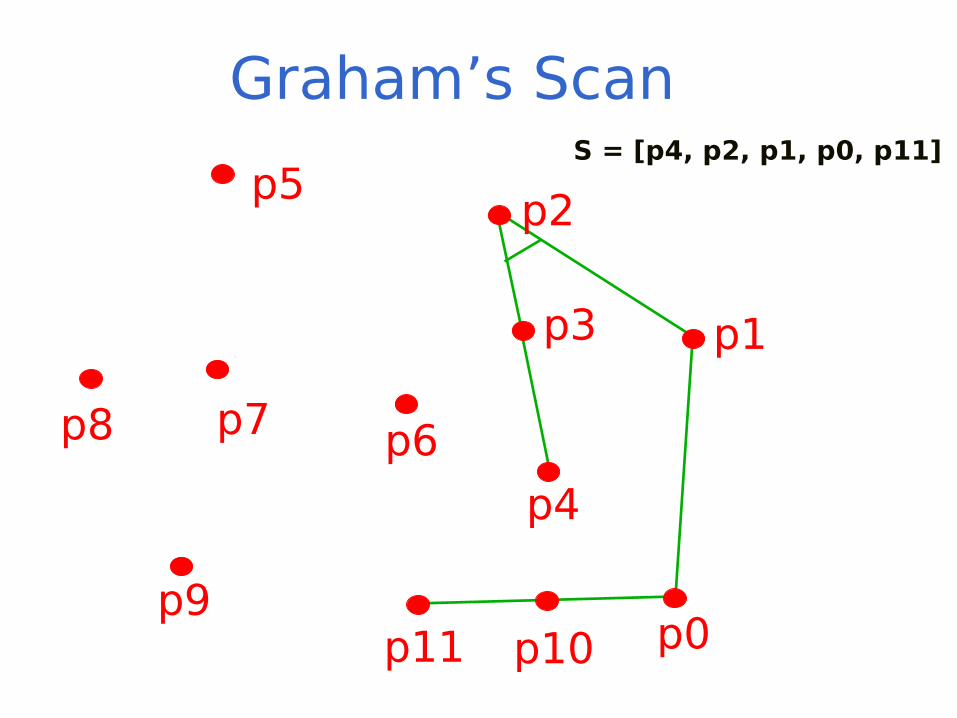
S = [p4, p2, p1, p0, p11]
p7
Graham’s Scan
p0
p1
p2
p3
p4
p5
p6p8
p9p10p11
S = [p10, p9, p8, p5, p2, p1, p0, p11]
p7
Graham’s Scan
p0
p1
p2
p3
p4
p5
p6p8
p9p10p11
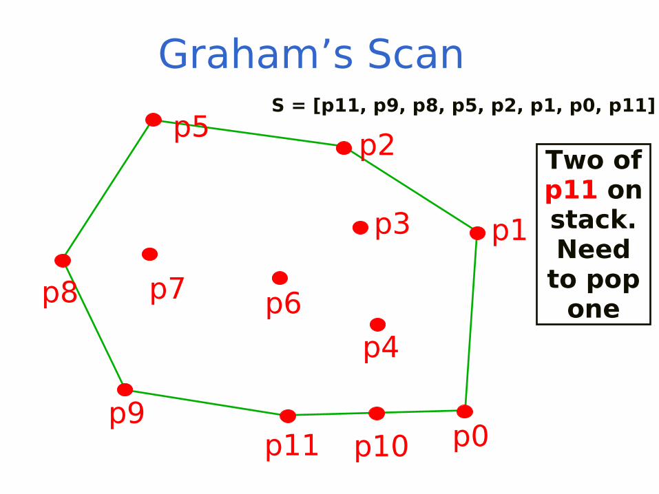
S = [p11, p9, p8, p5, p2, p1, p0, p11]
Two of p11 on stack.Need
to pop one
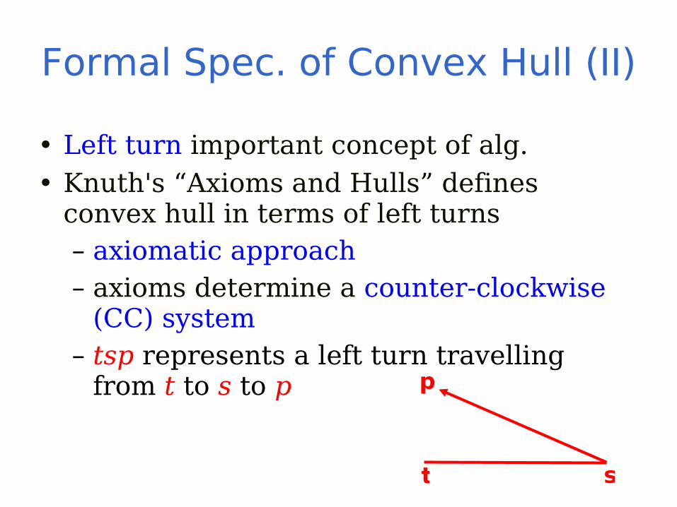
Formal Spec. of Convex Hull (II)
• Left turn important concept of alg.• Knuth's “Axioms and Hulls” defines
convex hull in terms of left turns– axiomatic approach– axioms determine a counter-clockwise
(CC) system– tsp represents a left turn travelling
from t to s to p
t s
p
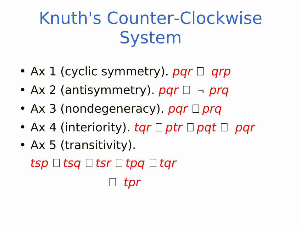
Knuth's Counter-Clockwise System
• Ax 1 (cyclic symmetry). pqr ⇒ qrp
• Ax 2 (antisymmetry). pqr ⇒ ¬ prq
• Ax 3 (nondegeneracy). pqr ∨ prq
• Ax 4 (interiority). tqr ∧ ptr ∧ pqt ⇒ pqr
• Ax 5 (transitivity).
tsp ∧ tsq ∧ tsr ∧ tpq ∧ tqr
⇒ tpr
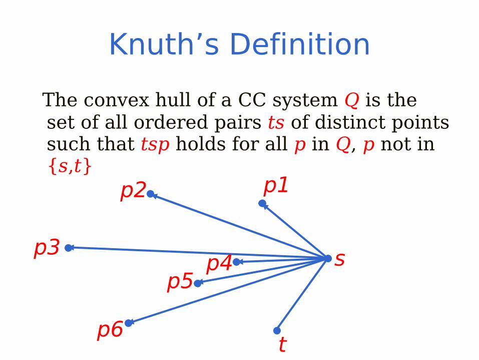
Knuth’s Definition
The convex hull of a CC system Q is the set of all ordered pairs ts of distinct points such that tsp holds for all p in Q, p not in {s,t}
t
s
p1p2
p3p4
p5
p6
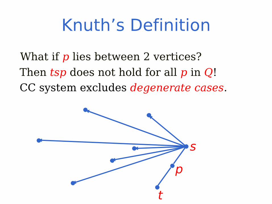
Knuth’s Definition
What if p lies between 2 vertices?
Then tsp does not hold for all p in Q! CC system excludes degenerate cases.
t
s
p

Extension to CC System
• To permit collinear points, notion of betweenness introduced
• Axioms updated to incorporate this change
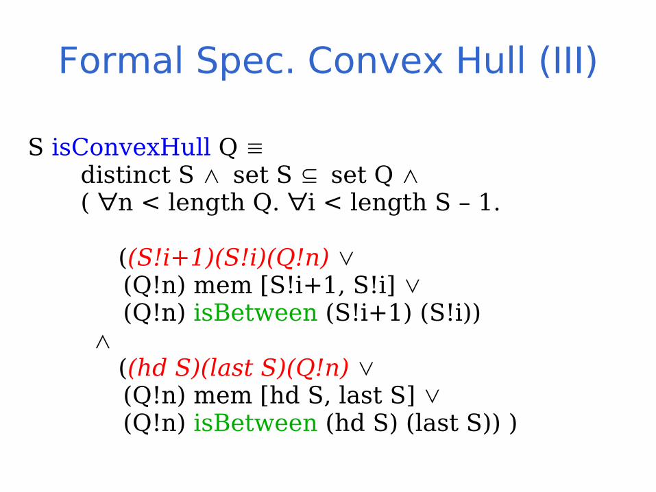
Formal Spec. Convex Hull (III)
S isConvexHull Q distinct S ∧ set S ⊆ set Q ∧ ( ∀n < length Q. ∀i < length S – 1.
((S!i+1)(S!i)(Q!n) ∨ (Q!n) mem [S!i+1, S!i] ∨ (Q!n) isBetween (S!i+1) (S!i))
∧ ((hd S)(last S)(Q!n) ∨ (Q!n) mem [hd S, last S] ∨ (Q!n) isBetween (hd S) (last S)) )
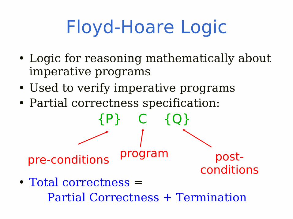
Floyd-Hoare Logic
• Logic for reasoning mathematically about imperative programs
• Used to verify imperative programs• Partial correctness specification: {P} C {Q}
• Total correctness = Partial Correctness + Termination
pre-conditions program post-conditions
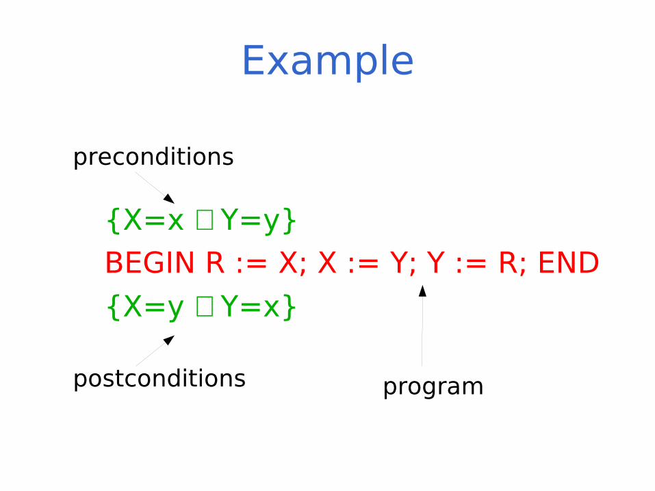
Example
{X=x ∧ Y=y}
BEGIN R := X; X := Y; Y := R; END
{X=y ∧ Y=x}
preconditions
postconditions program

Floyd-Hoare Logic (II)
• Partial correctness specification is annotated with mathematical statementscalled a loop invariant– loop invariant is the facts which remain
true every time a loop is entered or left
• Verification conditions (VCs) are then produced by the logic
• VCs provable → specification correct
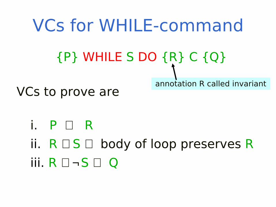
VCs for WHILE-command
{P} WHILE S DO {R} C {Q}
VCs to prove are
i. P ⇒ R
ii. R ∧ S ⇒ body of loop preserves R
iii. R ∧ ¬S ⇒ Q
annotation R called invariant
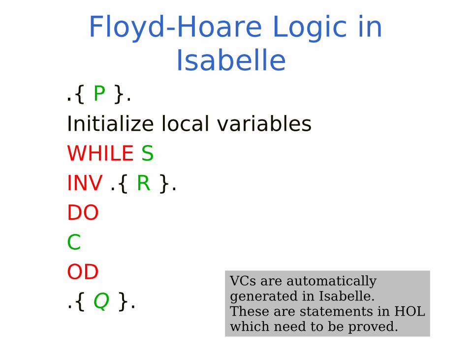
Floyd-Hoare Logic in Isabelle
.{ P }. Initialize local variables WHILE S INV .{ R }. DO C OD .{ Q }.
VCs are automatically generated in Isabelle.These are statements in HOLwhich need to be proved.
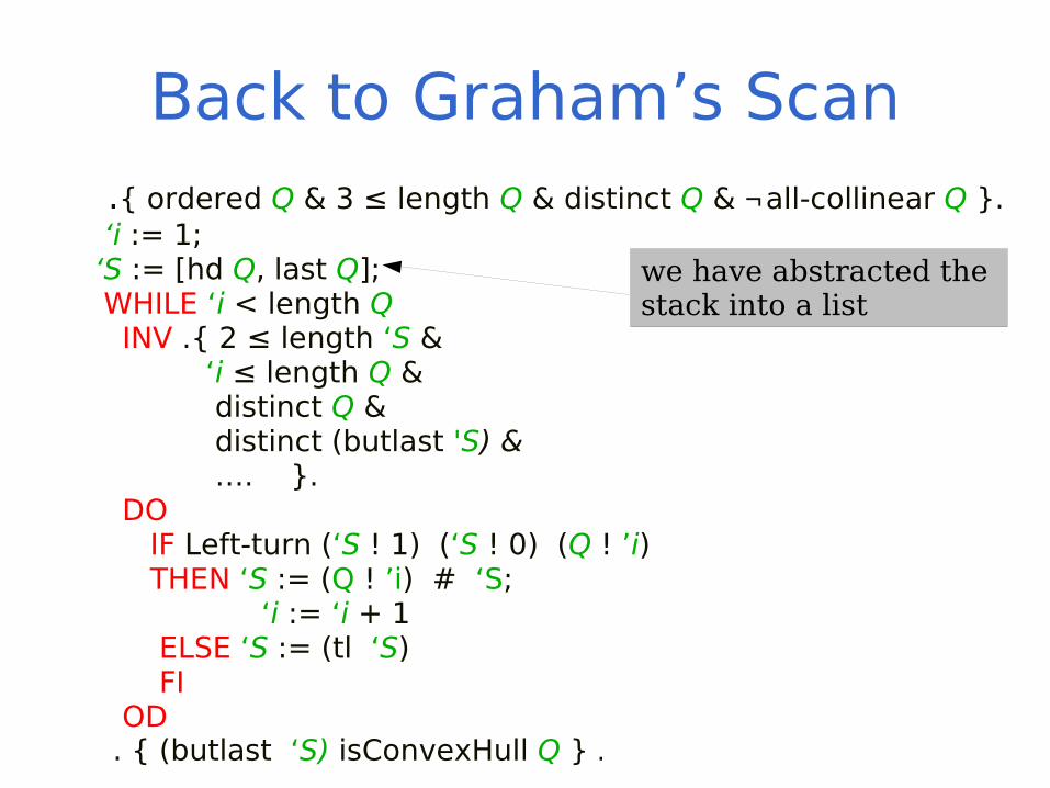
Back to Graham’s Scan .{ ordered Q & 3 ≤ length Q & distinct Q & ¬all-collinear Q }. ‘i := 1; ‘S := [hd Q, last Q]; WHILE ‘i < length Q INV .{ 2 ≤ length ‘S & ‘i ≤ length Q & distinct Q & distinct (butlast 'S) & …. }. DO IF Left-turn (‘S ! 1) (‘S ! 0) (Q ! ’i) THEN ‘S := (Q ! ’i) # ‘S; ‘i := ‘i + 1 ELSE ‘S := (tl ‘S) FI OD . { (butlast ‘S) isConvexHull Q } .
we have abstracted the stack into a list
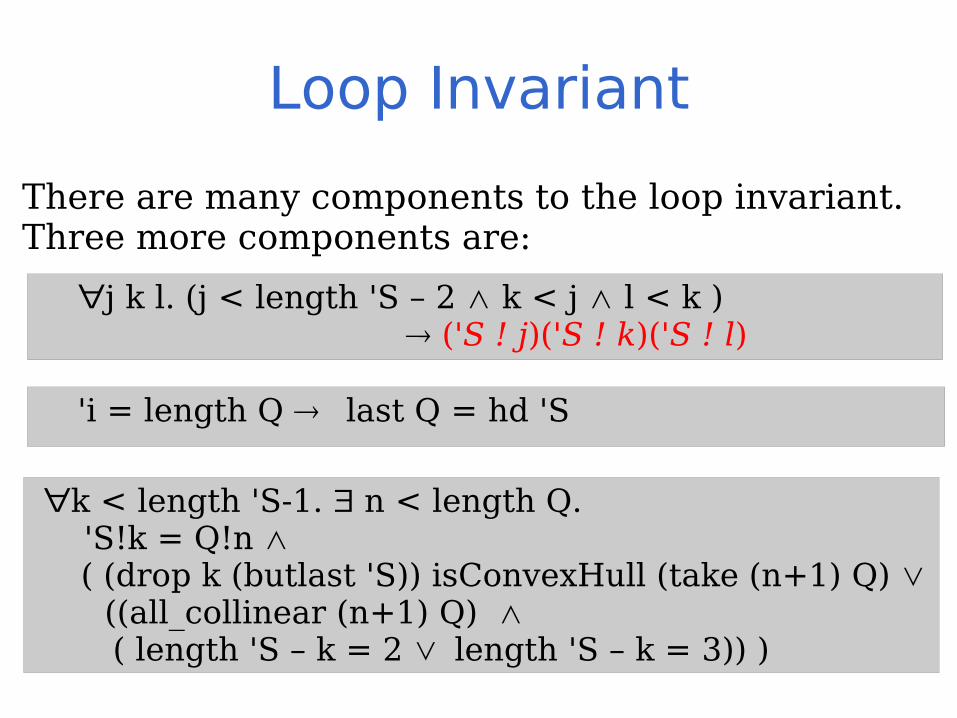
Loop Invariant
There are many components to the loop invariant.Three more components are:
∀j k l. (j < length 'S – 2 ∧ k < j ∧ l < k ) ('S ! j)('S ! k)('S ! l)
∀k < length 'S-1. n < length Q. 'S!k = Q!n ∧ ( (drop k (butlast 'S)) isConvexHull (take (n+1) Q) ∨ ((all_collinear (n+1) Q) ∧ ( length 'S – k = 2 ∨ length 'S – k = 3)) )
'i = length Q last Q = hd 'S

Third VC Generated
iii. R ∧ ¬S ⇒ Q ¬'i < length Q ∧ 'i ≤ length Q ∧
('i = length Q last Q = hd 'S) ∧ ¬all-collinear Q ∧ ( ∀k < length 'S-1. n < length Q. 'S!k = Q!n ∧
( (drop k (butlast 'S)) isConvexHull (take (n+1) Q) ∨ ((all_collinear (n+1) Q) ∧ ( length 'S – k = 2 ∨ length 'S – k = 3)) )
(butlast 'S) isConvexHull Q
From assumptions 'i must be equal to length Q

Third VC Generated
iii. R ∧ ¬S ⇒ Q 'i = length Q ∧
('i = length Q last Q = hd 'S) ∧ ¬all-collinear Q ∧ ( ∀k < length 'S-1. n < length Q. 'S!k = Q!n ∧
( (drop k (butlast 'S)) isConvexHull (take (n+1) Q) ∨ ((all_collinear (n+1) Q) ∧ ( length 'S – k = 2 ∨ length 'S – k = 3)) )
(butlast 'S) isConvexHull Q
Can then infer: last Q = hd 'S, and instantiate: k = 0
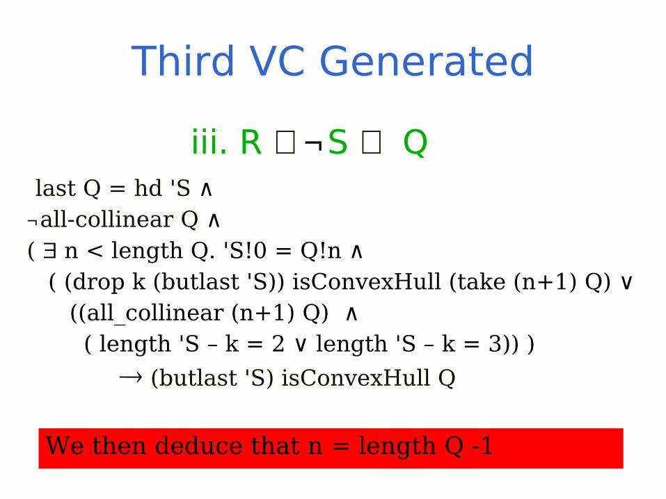
Third VC Generated
iii. R ∧ ¬S ⇒ Q last Q = hd 'S ∧ ¬all-collinear Q ∧ ( n < length Q. 'S!0 = Q!n ∧
( (drop k (butlast 'S)) isConvexHull (take (n+1) Q) ∨ ((all_collinear (n+1) Q) ∧ ( length 'S – k = 2 ∨ length 'S – k = 3)) )
(butlast 'S) isConvexHull Q
We then deduce that n = length Q -1
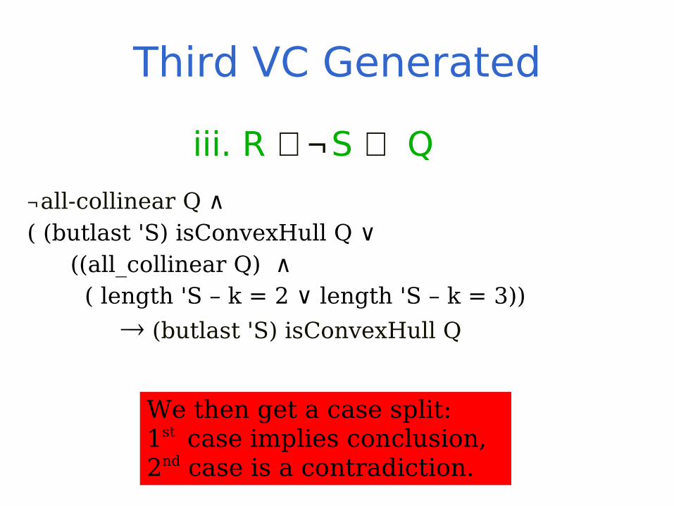
Third VC Generated
iii. R ∧ ¬S ⇒ Q ¬all-collinear Q ∧ ( (butlast 'S) isConvexHull Q ∨ ((all_collinear Q) ∧ ( length 'S – k = 2 ∨ length 'S – k = 3))
(butlast 'S) isConvexHull Q
We then get a case split: 1st case implies conclusion, 2nd case is a contradiction.

Remarks on Proof • Discovering correct loop invariant is:
– difficult, iterative process of refining– hindered due to Emacs PG's poor support
for re-factoring
• Writing own tactics/automation is challenging– can be aided by FeaSch-on-Isabelle
• Alternative to axiomatic approach?– Isabelle methodology prefers theories to be
conservative extensions of the library– We could define left turn!
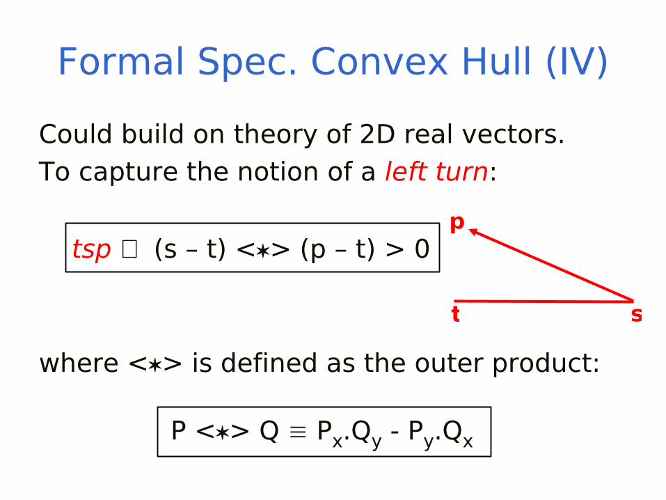
Formal Spec. Convex Hull (IV)
Could build on theory of 2D real vectors.To capture the notion of a left turn:
tsp ⇒ (s – t) <> (p – t) > 0
where <> is defined as the outer product:
P <> Q ≡ Px.Qy - Py.Qx
t s
p
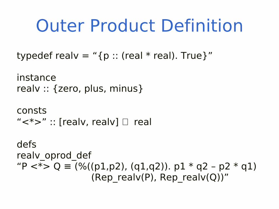
Outer Product Definition
typedef realv = “{p :: (real * real). True}”
instancerealv :: {zero, plus, minus}
consts“<*>” :: [realv, realv] ⇒ real
defsrealv_oprod_def“P <*> Q ≡ (%((p1,p2), (q1,q2)). p1 * q2 – p2 * q1) (Rep_realv(P), Rep_realv(Q))”
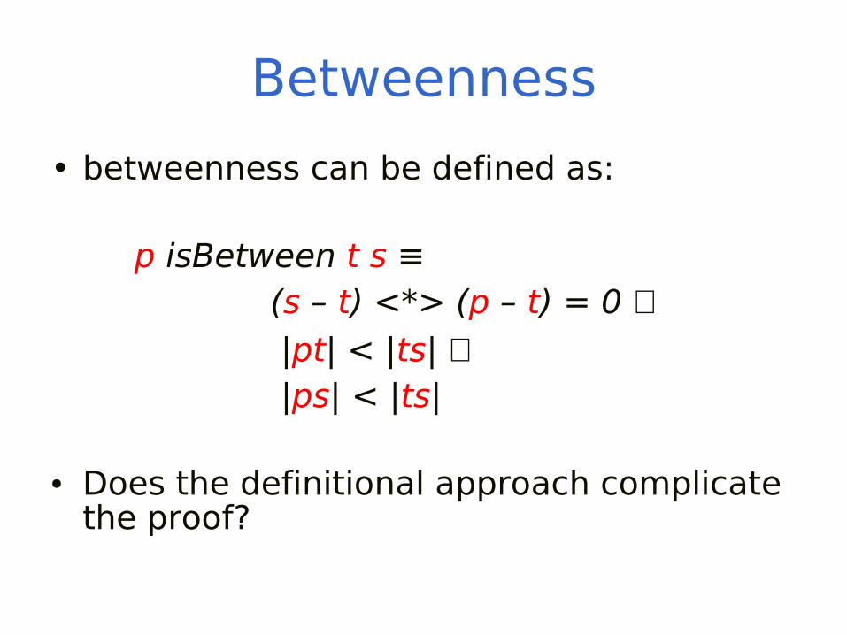
Betweenness
• betweenness can be defined as:
p isBetween t s ≡ (s – t) <*> (p – t) = 0 ∧ |pt| < |ts| ∧ |ps| < |ts|
● Does the definitional approach complicate the proof?

Proving Knuth's Axiom 5
• Proof breaks down into:– non-linear equations, difficult to solve – many case splits and tedious computation
• How can we ease the proving process?
Axiom 5. tsp ∧ tsq ∧ tsr ∧ tpq ∧ tqr ⇒ tpr
t s
p
q
r

Real Algebra
• Decidability for the first order theory of real closed fields is most fundamental result with respect to real numbers (shown by Tarski)
• Collins gave first practical decision algorithm for this problem
• However, no decision procedure within Isabelle
• But, QEPCAD can help:– CAD (Cylindrical Algebraic Decomposition)
– QEPCAD also gives a method for QE (Quantifier Elimination)
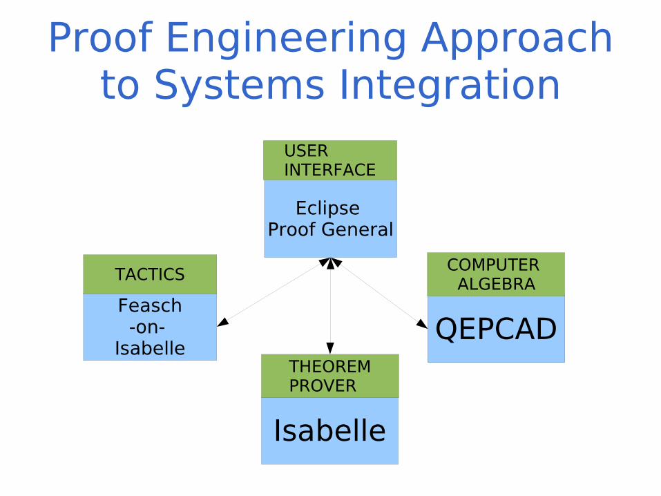
QEPCAD
Eclipse Proof General
Isabelle
QEPCADFeasch-on-
Isabelle
TACTICS
USER INTERFACE
COMPUTER ALGEBRA
THEOREMPROVER
Proof Engineering Approach to Systems Integration

Benefits of PE Approach
• Modularity and interoperability:– QEPCAD widget could work standalone– result available for many systems
• User has more control– setting parameters– changing translations (input and output)
• Greater inspectability


