
MATH 685/CSI 700 Lecture Notes
Lecture 1.
Intro to Scientific Computing
Useful info Course website:
http://math.gmu.edu/~memelian/teaching/Spring10 MATLAB instructions:
http://math.gmu.edu/introtomatlab.htm Mathworks, the creator of MATLAB: http://www.mathworks.com OCTAVE = free MATLAB clone
Available for download at http://octave.sourceforge.net/

Scientific computing Design and analysis of algorithms for numerically solving
mathematical problems in science and engineering
Deals with continuous quantities vs. discrete (as, say, computer science)
Considers the effect of approximations and performs error analysis
Is ubiquitous in modern simulations and algorithms modeling natural phenomena and in engineering applications
Closely related to numerical analysis

Develop mathematical model (usually requires a combination of math skills and some a priori knowledge of the system)
Come up with numerical algorithm (numerical analysis skills)
Implement the algorithm (software skills)
Run, debug, test the software
Visualize the results
Interpret and validate the results
Computational problems:attack strategy
Mathematical modeling

Computational problems:well-posedness The problem is well-posed, if
(a) solution exists
(b) it is unique
(c) it depends continuously on problem data
The problem can be well-posed, but still sensitive to perturbations. The algorithm should attempt to simplify the problem, but not make sensitivity worse than it already is.
Simplification strategies:
Infinite finite
Nonlinear linear
High-order low-orderOnly
approximate
solutio
n can be
obtained this
way!

Sources of numerical errors Before computation
modeling approximations empirical measurements, human errors previous computations
During computation truncation or discretization Rounding errors
Accuracy depends on both, but we can only control the second part Uncertainty in input may be amplified by problem Perturbations during computation may be amplified by algorithm
Abs_error = approx_value – true_valueRel_error = abs_error/true_value
Approx_value = (true_value)x(1+rel_error)
Can be controlled througherror analysis
Cannot be controlled

Sources of numerical errors Propagated vs. computational error
x = exact value, y = approx. value F = exact function, G = its approximation G(y) – F(x) = [G(y) - F(y)] + [F(y) - F(x)]
Rounding vs. truncation error Rounding error: introduced by finite precision calculations in the
computer arithmetic Truncation error: introduced by algorithm via problem simplification, e.g.
series truncation, iterative process truncation etc.
Total error = Computational error:affected by algorithm
Propagated data error:not affected by algorithm+
Computational error = Truncation error + rounding error
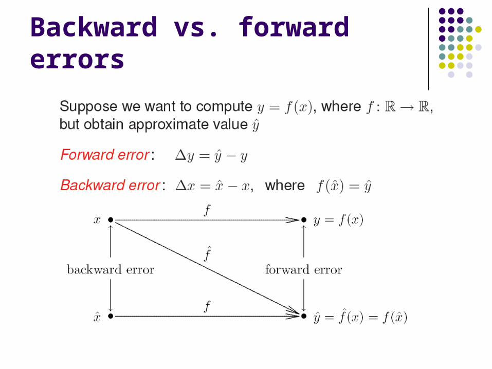
Backward vs. forward errors
Backward error analysis How much must original problem change to give result actually
obtained?
How much data error in input would explain all error in computed result?
Approximate solution is good if it is the exact solution to a nearby problem
Backward error is often easier to estimate than forward error

Backward vs. forward errors

Conditioning Well-conditioned (insensitive) problem: small relative change in
input gives commensurate relative change in the solution Ill-conditioned (sensitive): relative change in output is much larger
than that in the input data Condition number = measure of sensitivity
Condition number = |rel. forward error| / |rel. backward error|
= amplification factor

Conditioning
Stability Algorithm is stable if result produced is relatively insensitive to
perturbations during computation
Stability of algorithms is analogous to conditioning of problems
From point of view of backward error analysis, algorithm is stable if result produced is exact solution to nearby problem
For stable algorithm, effect of computational error is no worse than effect of small data error in input

Accuracy Accuracy : closeness of computed solution to true solution of problem
Stability alone does not guarantee accurate results
Accuracy depends on conditioning of problem as well as stability of algorithm
Inaccuracy can result from applying stable algorithm to ill-conditioned problem or unstable algorithm to well-conditioned
problem
Applying stable algorithm to well-conditioned problem yields accurate solution

Floating point representation

Floating point systems

Normalized representation
Not all numbers can be represented this way, those that can are called machine numbers

Rounding rules If real number x is not exactly representable, then it is approximated by
“nearby” floating-point number fl(x)
This process is called rounding, and error introduced is called rounding error
Two commonly used rounding rules chop: truncate base- expansion of x after (p − 1)st digit; also called round toward zero round to nearest : fl(x) is nearest floating-point number to x, using floating-
point number whose last stored digit is even in case of tie; also called round to even
Round to nearest is most accurate, and is default rounding rule in IEEE systems
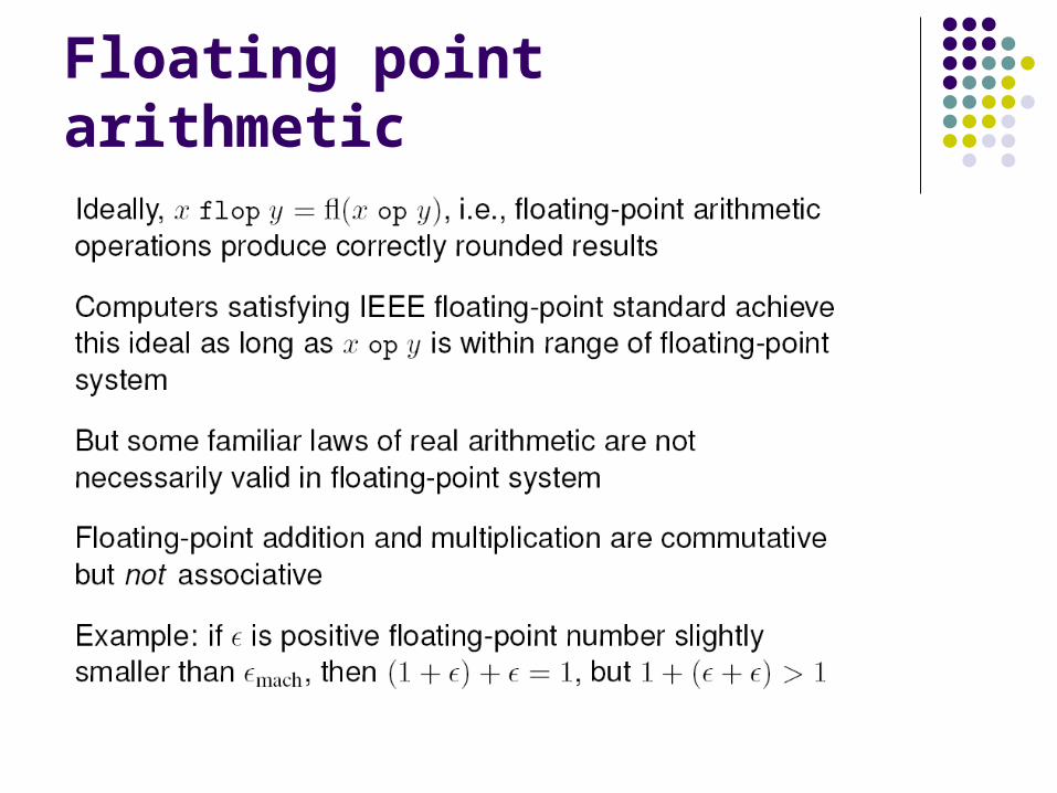
Floating point arithmetic

Machine precision

Floating point operations

Summing series in floating-point arithmetic

Loss of significance
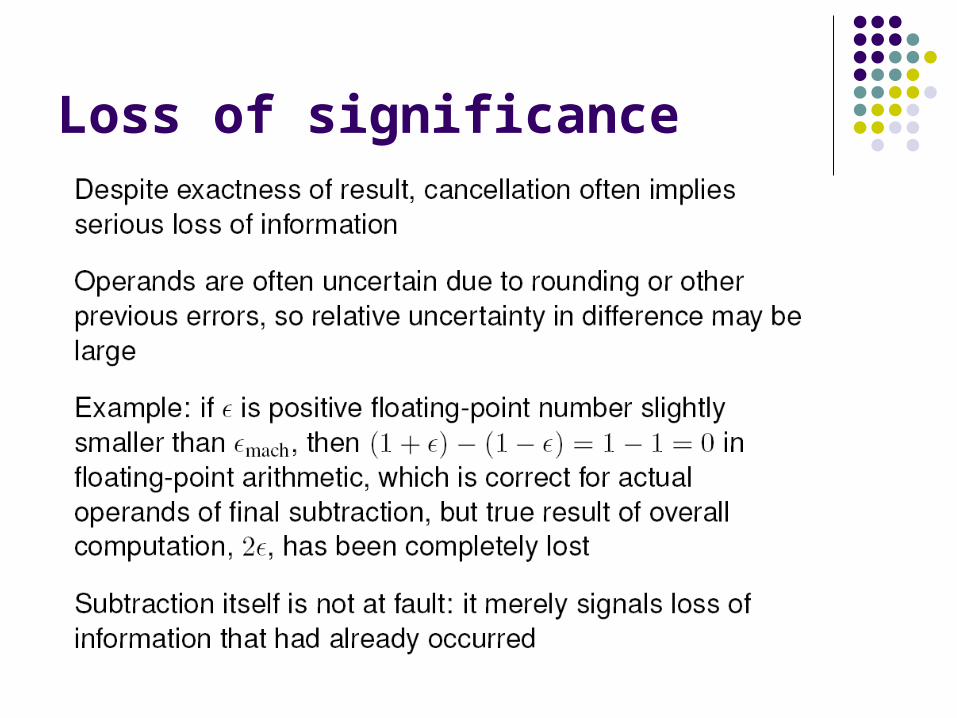
Loss of significance
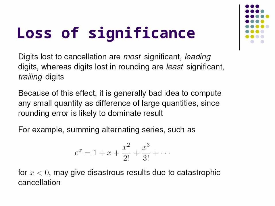
Loss of significance
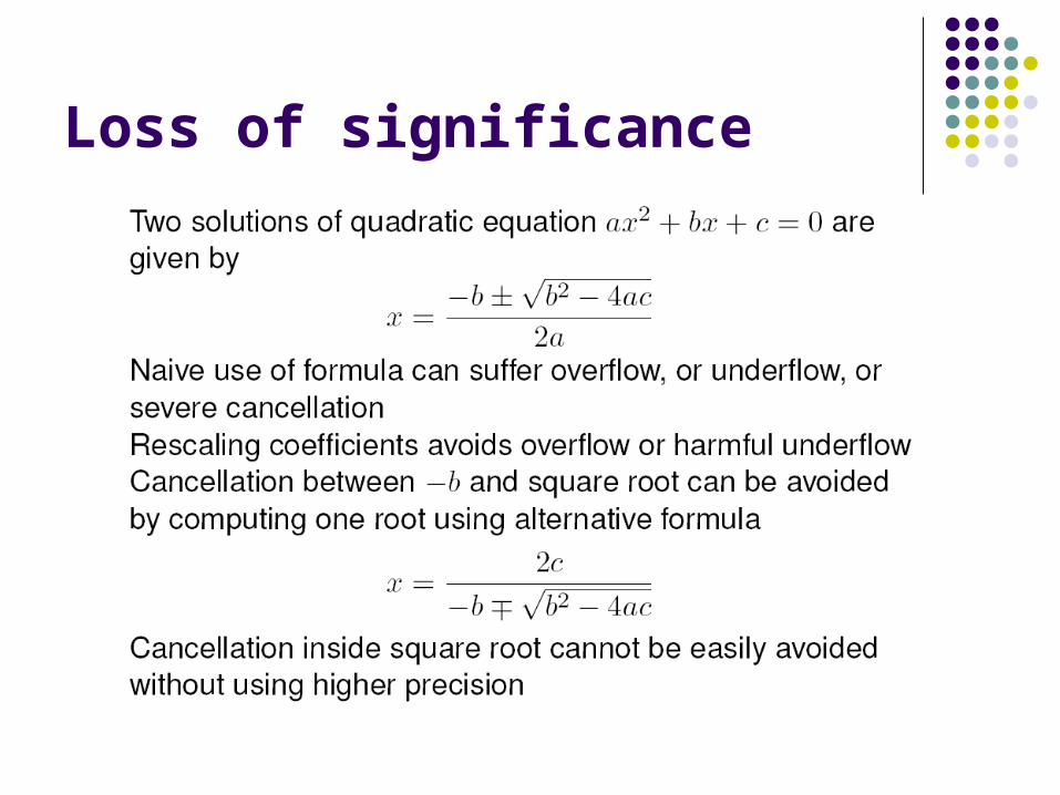
Loss of significance


![CS485/685 Lecture 6: Jan 21, 2016CS485/685 Lecture 6: Jan 21, 2016 Linear Regression by Maximum Likelihood, Maximum A Posteriori and Bayesian Learning [B] Sections 3.1 –3.3, [M]](https://cdn.vdocuments.us/doc/165x107/5f2fa31c890ecc77d5623d7b/cs485685-lecture-6-jan-21-2016-cs485685-lecture-6-jan-21-2016-linear-regression.jpg)


