
National Aeronautics and Space Administration
Erika Podest and Amita Mehta
19 November 2018
Mapping the Kerala Floods with SAR

NASA’s Applied Remote Sensing Training Program 2
Objectives
By the end of this exercise, you will: • Know where to access SAR data• Know how to use the Sentinel-1 Toolbox to process SAR data• Be able to generate a flooding classification from a SAR image

NASA’s Applied Remote Sensing Training Program 3
Requirements
• Sentinel Toolbox installed in your computer– http://step.esa.int/main/download/

NASA’s Applied Remote Sensing Training Program 4
Note
This is a two-part exercise:• Part 1 will focus on access and processing of Sentinel-1 SAR data• Part 2 will focus on generating a flooding classification map

NASA’s Applied Remote Sensing Training Program 5
Part 1: Outline
• Download Sentinel-1 images through the Alaska Satellite Facility website• Subset the image• Perform radiometetric correction• Apply a speckle filter• Perform geometric correction

NASA’s Applied Remote Sensing Training Program 6
Sentinel-1 Coverage
• Sentinel-1– Two satellites: A & B– Each satellite has global coverage
every 12 days– Global coverage of 6 days over the
equator when using data from both satellites

NASA’s Applied Remote Sensing Training Program 7
Sentinel-1: Modes of Acquisition
1. Extra Wide Swath – for monitoring oceans and coasts
2. Strip Mode – by special order only and intended for special needs
3. Wave Mode – routine collection for the ocean
4. Interferometric Wide Swath – routine collection for land
NASA’s Applied Remote Sensing Training Program 8
How to Access Sentinel-1 Images
• Alaska SAR Facility– http://www.asf.alaska.edu/sentinel/
• European Space Agency Portal– http://sentinel.esa.int/web/sentinel-data-access/access-to-sentinel-data/

NASA’s Applied Remote Sensing Training Program 9
Sentinel-1 Toolbox
• An open source software developed by ESA for processing and analyzing radar images from different satellites
• Includes the following tools– Calibration– Speckle noise– Terrain correction– Mosaic production– Polarimetry– Interferometry– Classification

Accessing, Opening and Displaying SAR Data

NASA’s Applied Remote Sensing Training Program 11
Accessing Sentinel-1 Data
1. Go to the Alaska Satellite Facility Sentinel Data Portal: https://vertex.daac.asf.alaska.edu/
2. Identify your area (76.77,7.97,77.41,8.25,76.9,10.31,76.18,9.43,76.77,7.97)
3. Identify images of interest (Sentinel-1 A/B)
4. Click on Optional Search Criteria and specify July 1, 2018-Aug. 30, 2018
5. Click on Search at the bottom of the page

NASA’s Applied Remote Sensing Training Program 12
Accessing Sentinel-1 Data
5. Select granule S1A_IW_GRDH_1SDV_20180704T004106_20180704T004131_022637_0273E1_B4B0 from Jul. 4, 2018. Path 165 Frame 563. This image represents conditions before the flood.
6. Download the L1 Detected High-Res Dual-Pol (GRD-HD) Product7. Select granule
S1A_IW_GRDH_1SDV_20180821T004109_20180821T004134_023337_0289D5_B2B2 from Aug. 21, 2018. Path 165 Frame 563. This image represents conditions after the flood.
8. Download the L1 Detected High-Res Dual-Pol (GRD-HD) Product

NASA’s Applied Remote Sensing Training Program 13
Accessing Sentinel-1 Data

NASA’s Applied Remote Sensing Training Program 14
Opening the Data with the Sentinel Toolbox
1. Initiate the Sentinel Toolbox by clicking on its desktop icon2. In the Sentinel Toolbox interface, go to the File menu and select Open Product3. Select the folder containing your Sentinel-1 file, and double click on the .zip file
(do not unzip the file; the program will do it for you)4. Open the second file
NASA’s Applied Remote Sensing Training Program 15
Opening the Data with the Sentinel Toolbox
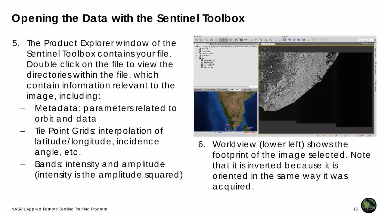
5. The Product Explorer window of the Sentinel Toolbox contains your file. Double click on the file to view the directories within the file, which contain information relevant to the image, including:
– Metadata: parameters related to orbit and data
– Tie Point Grids: interpolation of latitude/longitude, incidence angle, etc.
– Bands: intensity and amplitude (intensity is the amplitude squared)
6. Worldview (lower left) shows the footprint of the image selected. Note that it is inverted because it is oriented in the same way it was acquired.

NASA’s Applied Remote Sensing Training Program 16
Opening the Data with the Sentinel Toolbox- RGB Image
7. Go back to the Product Explorer tab8. Select the file name of the Sentinel-1 dataset. Afterwards, select Open RGB
Image Window to display a color image of VV, VH, and VV/VH ratio

NASA’s Applied Remote Sensing Training Program 17
Opening the Data with the Sentinel Toolbox- Pixel Information
• In the upper left window select “Pixel Info” to see the value and the lat/lon of each pixel in the image opened

Preprocessing

NASA’s Applied Remote Sensing Training Program 19
Data Preparation
• Select Raster and then Subset. Repeat the subset for the 2nd image.
Defining a Subset

NASA’s Applied Remote Sensing Training Program 20
Preprocessing: Geometric and Radiometric Calibration
• The objective in performing a calibration is to create an image where the value of each pixel is directly related with the backscatter of the surface.
• This process is essential for analyzing the images in a quantitative way. It is also important for comparing images from different sensors, modalities, processors or acquired at different times.

NASA’s Applied Remote Sensing Training Program 21
Example: Preprocessing – Radiometric Calibration
Select Radar > Radiometric > Calibrate. Run on each subset.
The main radiometric distortions are due to:
1. Signal loss as it propagates2. Non-uniform antenna pattern3. Difference in gain4. Saturation5. Speckle

NASA’s Applied Remote Sensing Training Program 22
Example: Preprocessing – Speckle Filter
Select Radar > Speckle Filtering > Single Product. Apply to each subset.
• Speckle is part of radar images and makes interpretation difficult because the “salt and pepper” effect corrupts information about the surface
• There are many techniques to extract information from radar images that have lots of speckle– In this case, we will use the Lee filter
NASA’s Applied Remote Sensing Training Program 23
Example: Preprocessing – Geometric Calibration
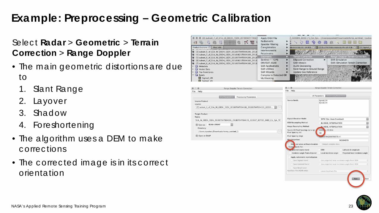
Select Radar > Geometric > Terrain Correction > Range Doppler• The main geometric distortions are due
to1. Slant Range2. Layover3. Shadow4. Foreshortening
• The algorithm uses a DEM to make corrections
• The corrected image is in its correct orientation

NASA’s Applied Remote Sensing Training Program 24
Example: Preprocessing – Geometric Calibrarion
• Select Radar > Geometric > Terrain Correction > Range Doppler

NASA’s Applied Remote Sensing Training Program 25
Data Preparation
• Select Radar > Coregistration > Stack Tools > Create Stack
Stack the Two Images

NASA’s Applied Remote Sensing Training Program 26
Data PreparationStack the Two Images
Load images Specify Product Geolocation

NASA’s Applied Remote Sensing Training Program 27
Data PreparationCreate Multi-Temporal RGB Images
R- Jul. 4 VVG- Aug. 21 VHB- Aug. 21 VV

NASA’s Applied Remote Sensing Training Program 28
Data Preparation
Convert values to dB and convert band so that the dB image created is saved. Repeat for all bands within the stack.

NASA’s Applied Remote Sensing Training Program 29
Example: Processing – Classifying Water and Land
1. Load the Aug. 21 VH dB image and analyze the image histogram in the lower left window
2. Identify a threshold between high values and low values
3. Select the value that separates water from everything else. In this case it is -19.39 dB
NASA’s Applied Remote Sensing Training Program 30
Example: Processing – Classifying Water and Land
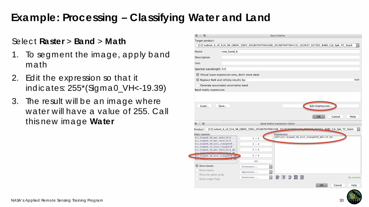
Select Raster > Band > Math1. To segment the image, apply band
math2. Edit the expression so that it
indicates: 255*(Sigma0_VH<-19.39)3. The result will be an image where
water will have a value of 255. Call this new image Water

NASA’s Applied Remote Sensing Training Program 31
Creating a Threshold to Separate Water and Land

NASA’s Applied Remote Sensing Training Program 32
Example: Processing – Classifying Water and Land
To change the colors, go to the color manipulation window on the bottom left and select Table. There you can assign a color to each of the 3 classes.

Supervised Classification

NASA’s Applied Remote Sensing Training Program 34
Training Area Selection
1. Select training areas by:– displaying the image as RGB– selecting from the main menu Vector > New Vector Data Container and
providing a name for your first training class (in this case permanent water)– in the Tools menu along the top bar, select the Polygon Drawing Tool – create a polygon of the area representative of open water.

NASA’s Applied Remote Sensing Training Program 35
Training Area Selection
2. Define the remaining training areas:– Repeat these same steps for each class:
• flood water, dry land, wet land

NASA’s Applied Remote Sensing Training Program 36
Running the Random Forest Classifier
3. Run the Random Forest Classification:– In the top menu, select Raster > Classification > Supervised Classification >
Radom Forest Classifier– in the pop-up window, select the file that you want to classify. To load it, select
the add-opened files on the column on the right (the second one down). Load the calibrated, speckle filtered, terrain corrected file.
– The second tab, Random Forest Classifier, will have a list of the training areas selected. Keep the defaults. Run it.

NASA’s Applied Remote Sensing Training Program 37
Running the Random Forest Classifier
4. Display the results:– a new image with extension _RF will be added in the product explorer window.
Display the bands > labeled classes image– In the color manipulation tab of the bottom left window, assign the desired
colors to each class

NASA’s Applied Remote Sensing Training Program 38
Running the Random Forest Classifier
5. Accuracy assessment:– While Random Forest is running, a separate text window pops displaying the
classification validation results:

NASA’s Applied Remote Sensing Training Program 39
Refining Your Classification Results
6. Refine the classification results by Applying a Filter:

NASA’s Applied Remote Sensing Training Program 40
Refining Your Classification Results
7. Go to the Color Manipulation Window8. Under the Table tab assign numbers and colors to your classes

NASA’s Applied Remote Sensing Training Program 41
Refined Classification Results


