
Macroeconomic Impact of Population Aging in Japan:
A Perspective from an Overlapping Generations Model�
Ichiro Mutoy, Takemasa Odaz and Nao Sudox
Abstract
Due to a sharp decline in the fertility rate and a rapid increase in longevity, Japan�s
population aging is the furthest advanced in the world. In this study we explore the
macroeconomic impact of population aging using a full-�edged overlapping generations
model. Our model replicates well the time paths of Japan�s macroeconomic variables
from the 1980s to the 2000s and yields future paths for these variables over a long
horizon. We �nd that Japan�s population aging as a whole adversely a¤ects GNP
growth by dampening factor inputs. It also negatively impacts on GNP per capita and
�scal variables, especially in the future, mainly due to the decline in the fraction of the
population of working-age. For these �ndings, fertility rate decline plays a dominant
role as it reduces both labor force and saver populations. The e¤ects of increased
longevity on economic growth are expansionary, but relatively small. Our simulations
predict that the adverse e¤ects will expand during the next few decades. In addition
to closed economy simulations, we examine the consequences of population aging in
a small open economy setting. In this case a decline in the domestic capital return
encourages investment in foreign capital, mitigating the adverse e¤ects of population
aging on GNP.
JEL Classi�cation: E20, J11
Keywords: Population Aging; Overlapping Generations Model; Capital Flow.
�The authors are grateful to Kiyohiko Nishimura, Eiji Maeda, Selahattin ·Imrohoro¼glu, TakatoshiIto, Shinichi Fukuda, Tsutomu Watanabe, Kosuke Aoki, Kaoru Hosono, Daisuke Miyakawa, RobertDekle, Toshitaka Sekine, Koichiro Kamada, Hibiki Ichiue, Kozo Ueda, Naoko Hara, Daisuke Ikeda,and seminar participants at the Federal Reserve Bank of St. Louis, SWET 2012 in Kushiro, andJapan Center for Economic Research for their advice and comments. The views expressed in thispaper are those of the authors and do not necessarily re�ect the o¢ cial views of the Bank of Japan.
yDirector, Research and Statistics Department, E-mail: [email protected] Director, Research and Statistics Department, E-mail: [email protected], Financial System and Bank Examination Department, E-mail: [email protected].
1

1 Introduction
In recent years, much attention has been paid to the macroeconomic consequences of pop-
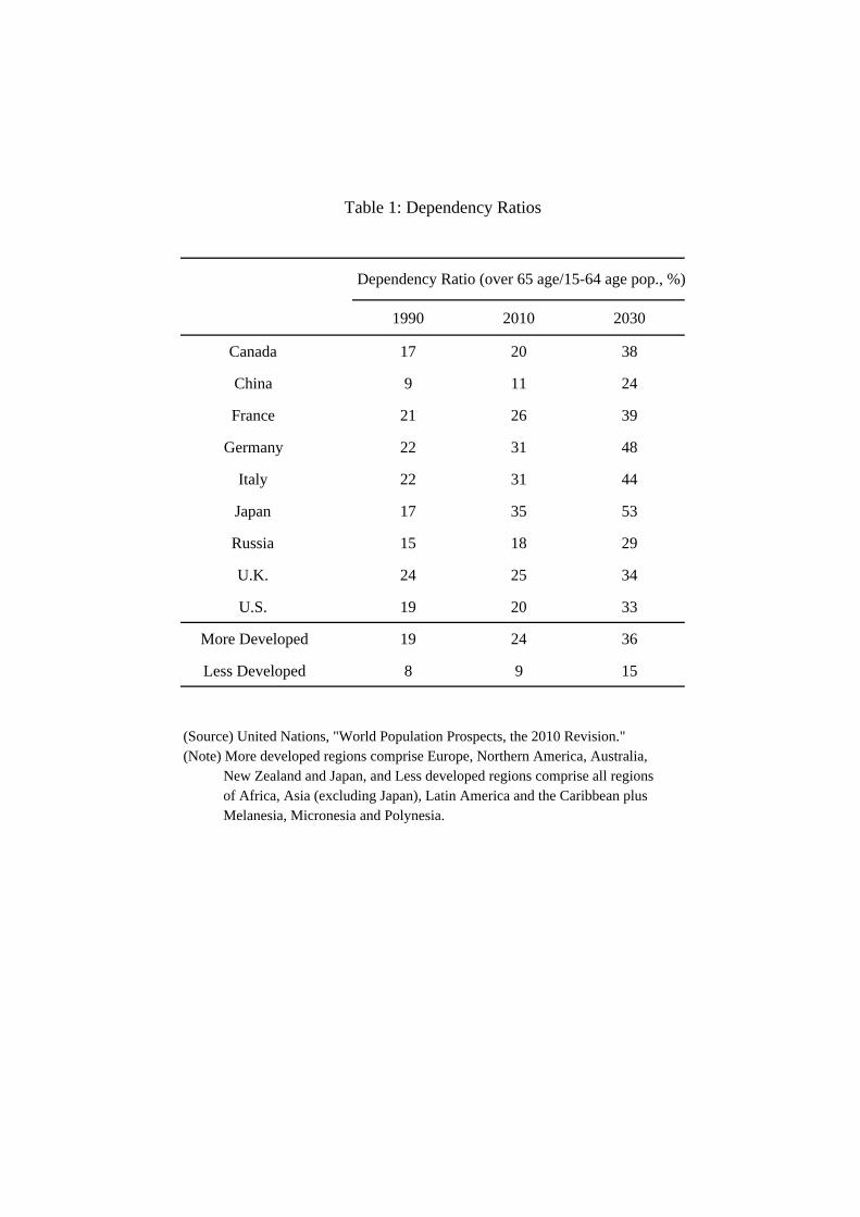
ulation aging across the world. Table 1 displays the dependency ratios for G7 countries as
well as developing countries, based on projections reported by the United Nations.1 The
dependency ratio exhibits a clear upward trend in all countries. In particular, Japan is
ahead of other countries in terms of the pace of its population aging. In 1990 Japan�s
dependency ratio was 17%, which was the lowest among G7 countries. However, it went
up to 35% in 2010, the highest in the group, and is expected to increase to 53% in 2030.
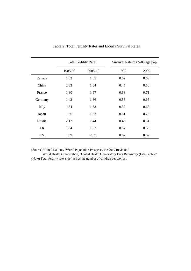
The rise in the dependency ratio stems from two factors: (i) a decline in the fertility rate
and (ii) an increase in longevity. Table 2 shows that Japan�s population aging has been
most rapid due to its lower fertility rate and greater longevity, respectively the lowest and
highest among listed countries in recent years. Japan can be seen as an illustrative example
for population aging.
There is vast literature exploring the link between demographic composition and eco-
nomic activity. One pioneering work within a general equilibrium framework is Auerbach
and Kotliko¤ (1987), who build an Overlapping Generations (hereafter OG) model cali-
brated to the U.S. economy and evaluate the impact of demographic transitions on eco-
nomic activity. They demonstrate that the OG model is considered the workhorse model
for analyzing the economic consequences of demographic transitions and the associated
�scal policy. Miles (1999) also utilizes an OG model to explore demographic impact, fo-
cusing on the U.K. and European countries.2 In recent years Japan�s population aging has
been investigated based on an OG model in two strands of literature.3 The one strand
focuses on movements in the saving rate in Japan. The Japanese saving rate has displayed
1Here the dependency ratio is de�ned as the �old-age�dependency ratio, the number of individuals agedabove 64 divided by the number of individuals aged 15 to 64.
2Within a growth accounting framework, for instance, Maddaloni et al. (2006) analyze the e¤ects ofpopulation aging on economic growth, �nancial markets and public �nance in the Euro area, consideringthe fertility rate, longevity, and immigration.
3As more recent work, Ikeda and Saito (2012) analyze, based on a dynamic stochastic general equilibriummodel, the implications of demographic changes for real interest rate dynamics in post-war Japan. From adi¤erent perspective, Fujiki et al. (2012) conduct an empirical investigation of how population aging a¤ectshouseholds�asset portfolio allocations, particularly between stocks and other assets, in Japan.
2
a downward trend since the 1990s, while it was much higher than the U.S. saving rate
in the past.4 Chen et al. (2007) and Braun et al. (2009) demonstrate that this can be
partially accounted for by population aging. Other things being equal, since a lower saving
rate results in less capital accumulation, the saving rate decline associated with population
aging may cause output decline. The other strand, for example, Ihori et al. (2005, 2011),
focuses on the e¤ects of population aging on the �scal balance including public pension
and health insurance systems, as well as on debt sustainability.5 If de�cits in these systems
are to some extent �nanced by the general government through distortional taxes, then
population aging may severely dampen private economic activity.
In this study, we investigate quantitatively the overall impact of population aging on
output and �scal variables from the 1980s and beyond. Our study provides a clear pic-
ture of economic outlooks in aging countries using a full-�edged OG model calibrated to
the Japanese economy where population aging is proceeding at the fastest pace in the
world. Our analysis incorporates two new ingredients into otherwise standard OG mod-
els. First, we explicitly introduce public medical bene�ts provided by a health insurance
system. Since the current health insurance system in Japan is partly organized in a pay-
as-you-go style similar to the public pension system, an increase in public medical bene�ts
due to population aging raises the payroll income tax rate, a¤ecting households�choice of
consumption and leisure. Most existing studies do not explicitly incorporate this aspect,
and thus potentially underestimate the impact of population aging on output and �scal
variables.6 Second, we adopt the �bond-in-utility�speci�cation developed in Hansen and
·Imrohoro¼glu (2012), when incorporating government bonds into the model. In Japan, the
return on government bonds has been lower than the return on private capital, and the
4Horioka (1997), Horioka and Watanabe (1997), Dekle (2000), and Koga (2005) are examples of sophis-ticated empirical work providing evidence for the Japanese saving rate decline.
5Dekle (2003) and Kozu et al. (2003) o¤er a broad discussion. ·Imrohoro¼glu and Sudo (2011a, b) andBraun and Joines (2012) utilize neoclassical growth and OG frameworks to address these issues from variousangles.
6Most studies on the Japanese economy, including Cheng et al. (2007) and Braun et al. (2009), abstractfrom the public health insurance system. A few exceptions, for example, Ihori et al. (2005, 2011) andOguro and Shimasawa (2011, Chapter4) introduce Japanese public health insurance in an OG model.Their models, however, assume an exogenous labor supply and are therefore immune from the distortionarye¤ects of population aging on economic growth through the social security tax.
3
spread has widened since the middle of the 1990s in spite of the massive increase in public
debt. This fact re�ects a strong preference for holding government bonds in the domestic
private sector. Most existing studies assume that households are indi¤erent between gov-
ernment bonds and private capital. However, this assumption fails to capture the actual
movements in the return on government bonds and hence in the corresponding interest
repayments. In long-term projections especially, this assumption generates a tendency to
overestimate government debt levels and the corresponding national burden.7
Assuming perfect foresight in the model, we compute the equilibrium transition paths
of allocations and factor prices from 1982 onward. Our model successfully replicates the
actual time paths of GNP and other main macroeconomic variables, such as the national
saving rate and the real interest rate up until 2010. In addition, we make what we call
an out-of-sample baseline projection from 2011 onward based on a scenario where future
paths for exogenous variables are plausibly chosen. To evaluate quantitatively the impact
of population aging on the economy, we simulate the model under hypothetical scenarios in
which population aging is arrested in terms of �rst the fertility rate, and then longevity.8
We compare the equilibrium paths generated under the alternative scenarios with those
obtained under the baseline scenario. In order to clarify the mechanism through which
population aging a¤ects economic growth, we divide the e¤ects of population aging into
fertility-driven e¤ects and longevity-driven e¤ects. We evaluate not only the e¤ects on
GNP growth, but also the e¤ects on GNP per capita in order to isolate the mechanical
impact of lower population growth. In addition to simulations based on a closed economy
model, we explore the macroeconomic impact of population aging in an open economy
setting with complete capital mobility. To this end, we extend our baseline model to a
small open economy model to compute the responses of key macroeconomic variables to a
decline in the fertility rate and an increase in longevity.
7 In carrying out our long-term projections where the government debt to GNP ratio is endogenouslydetermined, we �nd that this assumption impedes the convergence of the computed equilibrium transitionpath. This suggests that introducing the spread between private capital and government bonds is crucialfor evaluating the sustainability of government debt.
8Since the youngest households in our model are 21 years old, we de�ne the �fertility rate�in the modelas the growth rate of the age-21 population. This de�nition is di¤erent from common de�nitions of the�total fertility rate�, expressing the average number of children per woman during her lifetime.
4
The remainder of this paper is organized as follows. Section 2 describes the setup of
our model. Section 3 explains the data sources and our calibration methodology. Section
4 provides our quantitative �ndings on the macroeconomic impact of Japan�s population
aging. Section 5 extends the model into an open economy setting. Section 6 concludes.
2 Model
In this section, we present our OG model. The economy consists of four types of agents:
households, �rm, social security system, and general government. We incorporate two new
features into an otherwise standard OG model: (i) a public medical bene�t provided by the
health insurance system and (ii) a �bond-in-utility�speci�cation as developed in Hansen
and ·Imrohoro¼glu (2012).
2.1 Demographics
The time period of the model is discrete and annual. The economy consists of 80 generations
of di¤erent ages denoted by j = 21; :::; 100. In each period t, a new generation aged 21 is
born into the economy, while the other existing generations each shift forward by one. The
oldest generation, j = 100, which we assume as the maximum age, dies out deterministically
in the subsequent period. The growth rate of the new generation (age-21 households) in
period t is denoted by �t; which we will hereafter refer to as the fertility rate in the model.
Then the age-21 population in period t, expressed as P21;t, is given by
P21;t = (1 + �t)P21;t�1: (1)
All households face a mortality risk that is common within the same cohort but may di¤er
across cohorts. They survive to the subsequent period with conditional survival probability
j;t, which is the probability that households aged j � 1 in period t� 1 survive to become
age j households in period t. Note that 101;t = 0 by assumption. Then the population,
5
Pj;t, and cohort share, �j;t, of age j households in period t are expressed as follows:
Pj;t = j;tPj�1;t�1; (2)
�j;t =Pj;tP100i=21 Pi;t
for j = 21; :::; 100: (3)
2.2 Households
Until mandatory retirement at age j = 65, households supply labor to �rms and earn
wage income according to their age-speci�c labor e¢ ciency from age 21 to 65.9 Working
households pay not only the usual labor income tax, but also payroll income taxes covering
social security bene�ts, namely their public pension and medical bene�ts, in every period.
Households aged j > 65 withdraw from the labor force, and receive public pension bene�ts
from the social security system. Households own capital and rent it to �rms throughout
their lives. They also purchase one-period government bonds issued by the general govern-
ment, and receive interest payments from the general government. They consume the rest
of their income.
In period T , newly born households, whose age is j in a subsequent period t � T�21+j,
choose sequences of consumption, labor, capital and bond holdings, to maximize their
expected lifetime utility (discounted by the subjective discount factor �):
max100Xj=21
�j�21
"jY
i=21
i;T�21+i
#u (cj;t; 1� hj;t; bj+1;t+1) ; (4)
subject to the budget constraints over their lifetime:
(1 + � c;t) cj;t + kj+1;t+1 + bj+1;t+1
=�1 + (1� �k;t) rKt
�kj;t + (1 + r
Bt )bj;t (5)
+(1� �h;t) (1� � s;t � �m;t)wt"jhj;t + � t + �t for j � 65;
9Currently, mandatory retirement in Japanese �rms is not necessarily at age 65, but is usually setbetween 60 and 65. In our projections, however, there is little labor supplied by those aged 63 to 65.The results of the analysis may therefore be expected to change little even if we lower the assumed age ofmandatory retirement by a few years.
6

(1 + � c;t) cj;t + kj+1;t+1 + bj+1;t+1
=�1 + (1� �k;t) rKt
�kj;t + (1 + r
Bt )bj;t + pbj;t + � t + �t for j > 65; (6)
where cj;t is consumption and hj;t is labor input. kj;t and bj;t denote capital and bond
holdings of age j households at the beginning of period t. wt is the wage rate, rKt is the
before-tax real rate of return on private capital, and rBt is the after-tax real rate of return
on government bonds. � c;t is the consumption tax rate, �h;t and �k;t are the tax rates on
income from labor and capital, and � t is a lump-sum transfer in period t.10 �t is a lump-
sum transfer associated with accidental bequests, which are left by households who die in
the preceding period t � 1. � s;t and �m;t are the payroll income tax rates (contribution
rates) for public pension and health insurance, respectively. pbj;t is public pension bene�ts
that retirees aged j in period t receive, described later. "j is age-speci�c labor e¢ ciency
from age 21 to 65, which we assume time-invariant. We assume that a new household born
in period t has no initial assets11: k21;t = b21;t = 0. In addition, no household surviving
to the maximum age 100 carries over any assets to the next period: k101;t = b101;t = 0,
so there is no bequest motive. We also assume that the government collects all accidental
bequests including capital income in period t�1; and redistributes them equally among all
households alive in period t. The total amount of accidental bequests in period t is given
by
�t =
101Xj=22
(1� j;t)��1 + (1� �k;t�1) rKt�1
kj�1;t�1 + (1 + r
Bt�1)bj�1;t�1
�Pj�1;t�1: (7)
Following Hansen and ·Imrohoro¼glu (2012), we introduce government bond holdings
into the utility function. The basic idea behind this �bond-in-utility� speci�cation is to
incorporate households�preference for the liquidity and safety characteristic of government
bonds.12 The functional form of households�utility is assumed to be separable in terms of
10This corresponds conceptually to what is categorized as the sum of the net current transfers and thecapital transfers in the Japanese National Income Account.11The borrowing constraint is not imposed on households�assets in our model. In other words, households
are allowed to borrow against their future income.12As an alternative speci�cation, some studies, such as Arai and Ueda (2012), introduce an exogenous
7
its arguments, which are given as
u (cj;t; 1� hj;t; bj+1;t+1) = log cj;t + t log (1� hj;t) + �t log bj+1;t+1 for j � 65; (8)
u (cj;t; 1� hj;t; bj+1;t+1) = log cj;t + �t log bj+1;t+1 for 65 < j < 100; (9)
u (cj;t; 1� hj;t; bj+1;t+1) = log cj;t for j = 100; (10)
where t and �t are time-variant variables representing households�preferences for leisure
and government bond holding in period t. Higher t or �t implies that households put a
higher value on leisure or government bond holding. When households receive utility from
government bond holding (�t > 0), the �rst order conditions of age j households in period
t with respect to government bond holdings yield the following equation:
(1� �k;t)rKt � rBt =�t�1�(1 + � c;t)
100�1Xj=21
�j;tcj;t
bj+1;t+1: (11)
This equation demonstrates that, other things being equal, the spread between private
capital and government bonds increases with the preference parameter �t and decreases
with the average ratio of government bonds to consumption. A higher preference for
government bonds (higher �t) leads to a wider spread and smaller interest repayments
by the general government. A higher government debt level relative to consumption level
lowers the marginal utility from government bond holding and thereby narrows the spread.
2.3 Firm
There is a representative �rm producing �nal goods with the Cobb-Douglas production
technology. In perfectly competitive spot-markets the �rm rents capital and hires labor
from households so as to maximize its pro�t:
max�t = AtK�t L
1��t �RtKt � wtLt; (12)
spread between private capital and government bonds. An important feature of our �bond-in-utility�modelis that the model�s spread is endogenous and its size is negatively related to the outstanding amount ofgovernment debt.
8

where � is the capital share of output, Kt is aggregate capital stock, Lt is aggregate labor
input, and Rt is the rental rate of private capital. At denotes the total factor productivity
(hereafter TFP) in period t, and we assume that the TFP grows at the rate of gt in every
period:
gt � (At=At�1)1=(1��): (13)
In equilibrium, the factor prices are given by
Rt = �At
�Kt
Lt
���1� rKt + �t; (14)
wt = (1� �)At�Kt
Lt
��; (15)
where �t is the depreciation rate of private capital. Aggregate demand for capital and
labor inputs are equalized to aggregate supply of these primary inputs, so as to clear the
respective markets in every period:
Kt =100Xj=21
Pj;tkj;t; (16)
Lt =65Xj=21
Pj;t"jhj;t: (17)
Here, the evolution of the aggregate capital stock is given by
Kt+1 = It + (1� �t)Kt; (18)
where It is aggregate investment in period t.
2.4 Social Security System
The social security system is divided into two sections: public pension and health insurance.
We assume that the public pension bene�t pbj;t provided to age j households in period t
depends on their historical wage income. It is proportional to the average wage income
that households receiving the bene�t earned during their working years. The public pension
bene�t provided by the social security system to a new retiree in period t, pb65+1;t, is de�ned
9

as
pb65+1;t � �1
65 + 1� 21
65Xi=21
wt+i�65�1"ihi;t+i�65�1; (19)
where � is the replacement ratio that determines the size of the public pension bene�t
relative to the past wages. The public pension bene�t that age j households in period t
receive is formulated as
pbj;t = 0 for j = 21; 22; :::; 65;
pbj;t = pb65+1;t+65+1�j for j = 65 + 1; :::; 100: (20)
The per-capita medical costs, denoted by mbj , are assumed to be di¤erent across age
j and time-invariant.13 The age-speci�c pro�le of the medical costs is exogenously given
and grows along a balanced growth path. We de�ne the medical bene�t mbj;t for age j
households in period t as follows:
mbj;t = (1 + gt)mbj;t�1 for t = 2; 3; :::; mbj;t = mbj for t = 1: (21)
For both public pension bene�ts and medical bene�ts, part of the costs is covered by the
general government, and the rest is covered by the relevant section of the social security
system. Taking as given the coverage ratios of transfers/expenditures �nanced by the
general government, which we denote as �s;t and �m;t, the social security system adjusts
the contribution rates for public pension and health insurance, � s;t and �m;t, so that budget
balance is separately maintained for both the public pension and health insurance in every
period:
� s;t =(1� �s;t)
P100j=65+1 Pj;tpbj;t
wtP65j=21 Pj;t"jhj;t
; (22)
�m;t =(1� �m;t)
P100j=21 Pj;tmbj;t
wtP65j=21 Pj;t"jhj;t
: (23)
13The main reason is due to data availability. The pro�le could reasonably be considered time-variantbecause of fast progress in medical technology.
10

2.5 General Government
The general government raises revenues by newly issuing one-period government bonds and
levying taxes on households�consumption, labor income, and capital income, to �nance
its spending that is the sum of government purchases, transfers/expenditures to the social
security system, interest repayments on government bonds, and other lump-sum transfers.
Taking the sequences of government revenues and spending as given, government bond
issuance is adjusted so that the following consolidated budget constraint holds in every
period:
(1 + rBt )Bt +Gt + �m;t
100Xj=21
Pj;tmbj;t + �s;t
100Xj=65+1
Pj;tpbj;t +
100Xj=21
Pj;t� t +
100Xj=21
Pj;t�t
= Bt+1 + � c;tCt + �h;t(1� � s;t � �m;t)wtLt + �k;trKt Kt; (24)
where Gt and Bt are government purchases and government bonds at the beginning of
period t, respectively. Note that the supply of government bonds is equalized to the sum
of households�bond holdings in each period:
Bt =
100Xj=21
Pj;tbj;t: (25)
2.6 Competitive Equilibrium
Given the initial distribution of private capital stock and government bonds fkj+1;0; bj+1;0g100j=21,
the paths of the �scal policy variables fGt; � t; � c;t; �k;t; �h;t; � s;t; �m;t; �s;t; �m;tg1t=0, demo-
graphics f�t; f j;tg100j=21g1t=0, TFP growth rate fgtg1t=0, depreciation rate f�tg1t=0, and pref-
erence disturbances f t; �tg1t=0; a competitive equilibrium consists of sequences of prices
fwt; rKt ; rBt g1t=0, allocations fCt; Lt; Kt; Btg1t=0, and households�decision rules ffcj;t; hj;t;
kj+1;t+1; bj+1;t+1g100j=21g1t=0 such that, in each period, (i) households maximize their lifetime
utility (4), subject to (5) and (6), given prices; (ii) the �rm maximizes its pro�ts, (12),
given prices; (iii) the budget constraints of the social security system and the general gov-
ernment, (22), (23), and (24), hold; (iv) the market clearing conditions hold for the capital
input, labor input, and government bonds, (16), (17), and (25); (v) the resource constraint
11
holds:
Yt � AtK�t L
1��t = Ct + It +Gt +
100Xj=21
Pj;tmbj;t; (26)
where Yt is aggregate output and Ct is aggregate consumption:
Ct =
100Xj=21
Pj;tcj;t: (27)
3 Data, Calibration, and Assumptions
We take 1982 as the starting point for our simulations, because this is the �rst year for
which national account series with a consistent set of de�nitions are available. The last
period for which we have data on all variables is 2010. The model thus employs observed
values of its exogenous inputs for the 1982-2010 period, and assumed values of these inputs
for 2011 and beyond. We assume that the economy will reach its steady state far in the
future, and carry out an iterative computation to calculate an equilibrium transition path
that connects the economy of 1982 and the long-run steady state. In this section, we
�rst discuss, in detail, the calibration of the model�s structural parameters, as well as the
de�nition and construction of the exogenous inputs used in both in-sample simulation and
projection. We then explain the assumptions about the �scal regime in the long-run that
guarantees the household and general government transversality conditions, as well as the
assumptions governing the long-run steady state values.
3.1 Constant Parameters
The calibrated constant parameters are given in Table 3. The three parameters �; �; and �
are constant throughout our analysis. Following closely the data construction methodology
proposed in Hayashi and Prescott (2002) and ·Imrohoro¼glu and Sudo (2011a, b), we use the
sample average for the income share of capital in GNP � from 1982 to 2010. We choose the
value of the subjective discount factor � so that our benchmark model replicates well the
time path of the capital-output ratio for the period from 1982 to 2010. The replacement
ratio � for the public pension is set to 0.3 so that the model can reproduce the historical
12

average of the actual pension bene�ts to GNP ratio from 1982 to 2010.
In addition, we assume that the age-speci�c labor e¢ ciency "j and age-speci�c medical
costs mbj are constant over time. The labor e¢ ciency values are taken from Braun et al.
(2009), while the values for individual medical costs are taken from the 2009 Report of
National Medical Expenditure (NME) by the Ministry of Health, Labour and Welfare.
3.2 Inputs of Exogenous Variables for 1982-2010 and Beyond
In order to conduct perfect foresight projections from 1982 and beyond, we need to specify
parameter values characterizing the demographic structure; these include the growth rate
of the age-21 population (i.e., �fertility rate�in our model) f�tg1t=1982, conditional survival
probability ff j;tg100j=21g1t=1982; and sequence of exogenous macroeconomic variables fGt=Yt;
� t=Yt; � c;t; �h;t; �k;t; �s;t; �m;t; �t; gt; t; �tg1t=1982: The detailed de�nition and construction
methodologies for these variables are given in Appendix A.
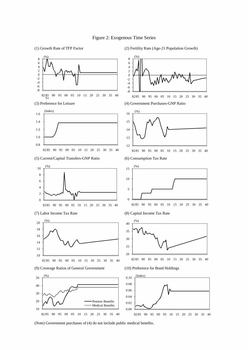
Figures 1 and 2 display, respectively, the age-speci�c life-cycle pro�les that characterize
households, and the time series of exogenous variables fed into the baseline model. As
in related studies on other countries, the labor e¢ ciency exhibits a hump-shape peaking
around age 55, the medical costs monotonically increase with age, and the conditional
survival probability decreases with age and grows steadily over time. The growth rate of
the age-21 population was above zero in the 1980s but has been continuously negative in
the current years, around -2%.
3.3 Steady State Assumptions
The calibrated steady state values of the key variables are presented in Table 4. In order
to ensure the transversality condition of the general government over a long horizon, and
to maintain the convergence of the dynamic paths in the economy, we consider, following
Hansen and ·Imrohoro¼glu (2012), a class of �scal regime switch that will take place in
2050. We assume that the general government adjusts the government bond issuance
endogenously from 1982 to 2049 so as to ful�ll the government budget constraint (24),
taking the sequence of the other �scal instrument variables fGt=Yt; � t=Yt; � c;t; �h;t; �k;t;
13
�s;t; �m;tg1t=1982 as given. From 2050 and beyond, the new �scal regime is implemented
and the general government adjusts the size of a lump-sum tax levied on all households
so as to maintain the government bond to GNP ratio at its target level. We assume that
the target level of the ratio decreases linearly from its value in 2050 to 0.441 by 2100, its
historical average over 1982 to 2010. Except for the growth rates of TFP and the age-21
population, the steady state values of the other variables are basically the sample averages
from 1982 to 2010. The steady state value of TFP growth is 1%, which is the historical
average of the growth rate of the Solow residual from 1995 to 2007.14
4 Quantitative Findings
In this section, we document the quantitative results of simulations. Under the baseline
assumptions, we conduct perfect foresight projections where newly-born households are
informed of the sequence of exogenous variables in their birth period and beyond. We �rst
demonstrate the in-sample performance of our model by comparing the model-generated
main macroeconomic variables with the data counterparts. We also provide out-of-sample
projections for 2011 onward. Next, we formulate counterfactual simulations to evaluate
the impact of population aging on GNP and the �scal balance. Since a decline in the
fertility rate and an increase in longevity are both important driving forces of Japan�s
population aging, we investigate these two e¤ects separately. In addition, we investigate
how in�uential the public health insurance system is in the aging Japan.
4.1 Baseline Long-Term Projection
We �rst demonstrate the basic performance of the model by comparing the actual and
model-generated series of key macroeconomic variables over the sample period 1982-2010.
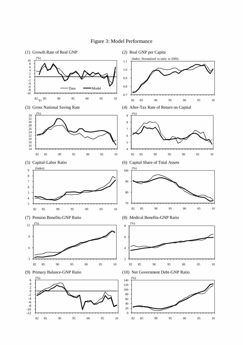
Figure 3 displays the time paths of the GNP growth rate, GNP per capita (de�ned as
real GNP per total population), national saving rate, real return on capital, capital-labor
14Here we drop the subsample periods that include the �bubble boom�during the 1980s and the global�nancial crisis from 2008 to 2009 in constructing our benchmark future path for TFP. The average valueover the whole sample period is 1.7%, which is slightly higher than our benchmark assumption. In AppendixC, we conduct a sensitivity analysis to see how our result is a¤ected by the assumption on TFP growth.
14

ratio, capital share of total assets, pension bene�ts to GNP ratio, medical bene�ts to GNP
ratio, primary balance to GNP ratio, and net government debt to GNP ratio. The thin
lines depict the actual series, and the thick lines depict the model-generated series. Our
model replicates the dynamics of the macroeconomic variables well. In particular, the
long-lasting output growth slowdown that started with the burst of the asset bubble in
1991 is reproduced in the model series. As discussed in existing studies such as Chen et
al. (2007) and Braun et al. (2009), the national saving rate and real return to capital also
decrease in the most recent two decades, and the model-generated data closely tracks the
corresponding actual time series. The general patterns of revenues and expenditures for
both the social security system and the general government are also captured by the present
model. In both actual data series and model-generated series, persistent increases in the
pension bene�t and medical bene�t, deterioration in the primary balance, and accelerated
government debt accumulation are observed.
Figure 4 shows out-of-sample projections for the macroeconomic variables from 2011
onwards under the baseline scenario. The Japanese economy experiences zero GNP growth
in the next decade, as 1% TFP growth is almost exactly o¤set by declines in labor and
capital inputs. From the late 2020s and beyond, however, GNP is seen to fall gradually,
since the factor inputs decline at a faster rate than before. As indicated by an increase
in average working hours in these periods, the reduction in the labor input is driven by
a decrease in the labor force population. A decline in the capital input is induced by
changes in households� saving behavior as well as an increased proportion of dis-savers.
Although workers raise their saving rate, the rise is dominated by the decline in the saving
rate of retirees. Redistribution by the general government will rise over a long horizon,
as shown in the expansion of public pension and medical bene�ts. Although the level of
GNP declines in the long-run, GNP per capita maintains a gradual increase, re�ecting the
increase in working hours and 1% TFP growth. Behind these movements, the after-tax rate
of return on private capital stays stable mainly because 1% TFP growth compensates for
the increase in the capital-labor ratio induced by population aging. On the other hand, the
real return on government bonds rises gradually over time because of deterioration in the
15

�scal balance caused by population aging. Consequently, the spread between private capital
and government bonds shrinks through the forecast horizon. Of course, this movement in
the spread depends strongly on the assumed future paths of households� preference for
government bond holding.15
4.2 Counterfactual Simulation
Next we examine how population aging a¤ects economic activity in Japan. To this end,
we conduct counterfactual simulations in which population aging is arrested. We investi-
gate separately the two e¤ects behind population aging in Japan, namely a decline in the
fertility rate and an increase in longevity. We also examine how in�uential public medical
burdens are in impacting on GNP and �scal variables in the aging Japan, by conduct-
ing a counterfactual experiment where a public health insurance system is not explicitly
incorporated as is the case with OG models commonly used in previous studies.
Decline in Fertility Rate
In Figure 5, we display the time paths of macroeconomic variables in the economy
where the population aged 21 is held constant from 1995 and beyond.16 This hypothetical
fertility rate sequence is substantially higher than the actual counterpart, which has been
almost continuously negative since 1995. The discrepancy between the baseline scenario,
denoted by the solid lines, and this counterfactual scenario, denoted by the dotted lines,
displays the quantitative contribution made by the decline in the fertility rate after 1995.
On the one hand, reduced fertility dampens GNP growth, the growth rates of the two factor
inputs, the national saving rate, and the capital return. On the other hand, it raises the
pension/medical bene�ts to GNP ratio. Its qualitative e¤ects on workers�saving behavior
and leisure choice change over the simulation period.
A fertility rate decline contributes to the slowdown of GNP growth through three
distinct channels. First, it mechanically reduces the labor force population. Second, by
15 In Appendix C, we conduct a sensitivity analysis to see how our result is a¤ected by the assumptionon households�preference for government bond holding.16This means that f�tg
1t=1995 = 0.
16

raising the proportion of retirees in the economy, it aggravates the social security burden
on labor income. As a result, the contribution rates, � s;t and �m;t, are raised so as to
satisfy the budget balance requirements of the social security system (22) and (23), thus
distorting workers� labor supply and saving decisions. Third, marginal propensities to
consume are higher among retirees than workers. On average, workers are savers and
retirees are dis-savers under both scenarios. The decline in the fertility rate, therefore,
increases the proportion of dis-savers among households, reduces the national saving rate,
and hampers capital accumulation. The �rst and third channels drive GNP growth down
primarily through reductions in the population of the labor force and savers. In contrast,
the second channel in�uences GNP growth by a¤ecting average working hours and the
workers�saving rate.
In the baseline scenario, the real return on capital is lowered as the labor input drops
more quickly than the capital input because of the fertility rate decline. Meanwhile, the
after-tax return on labor (the e¤ective wage) is reduced more as a result of higher con-
tribution rates. Average working hours and workers�capital saving rate are higher in the
baseline scenario than in the counterfactual scenario. In the baseline scenario working-age
households work more and save more because their lifetime income decreases substantially
due to the lower factor prices (e¤ective wage and return on capital) caused by the fertility
rate decline. As Figure 6 shows, GNP per worker is thus higher in the baseline scenario.
GNP per capita, however, is lower in the baseline scenario because the increase in GNP
per worker is more than cancelled out by the decline in the proportion of the working-age
population. This relative decrease in the working-age population is the dominant factor
depressing GNP per capita in the next few decades. It is noteworthy that these adverse
e¤ects on GNP per capita will expand sharply through the forecast horizon. Population ag-
ing also a¤ects the �scal balance negatively. Figure 7 displays the impact of a fertility rate
decline on the primary balance and net government debt level. The fertility rate decline
deteriorates the primary balance because it lowers tax revenues of the general government.
As a result, government debt accumulates more quickly over time.
17

Increase in Longevity
In Figure 8, we display the time paths of macroeconomic variables in the economy
where the household survival probability, instead of increasing, is held constant from 1982
onward.17 As shown in the upper panel of Figure 1, the conditional survival probability
shifts upward over time, with the increased survival probability of retirees being particularly
remarkable. The higher longevity impacts positively on variables such as the growth rates
of the two factor inputs, GNP growth, and GNP per capita, but not on the real rate of
return on capital or government bonds, nor on the retirees�saving rate.
Two reasons can be adduced to explain why increased longevity results in economic
expansion. The one reason is the absence of the predominant contractionary channel above
(the �rst of the three channels mentioned), which does not operate here since the labor
force population is almost una¤ected by a change in longevity. The other is the operation
of a further (the fourth) channel, through which increased longevity in�uences households�
precautionary motive. As pointed out in previous studies, such as Chen et al. (2007) and
Braun et al. (2009), households expecting to survive longer have an added incentive to work
and save so as to insure themselves against a longer life after retirement. Consequently,
average working hours and the capital saving rate of workers are both higher in the baseline
scenario. Admittedly, the second and third channels discussed above also operate when
longevity increases. As with the fertility rate decline, these channels dampen the hours
worked by younger generations and reduce the proportion of savers in the economy. Because
the increases in average working hours and saving rate stemming from the fourth channel
dominate the adverse e¤ects stemming from the second and third channels, GNP per capita
is higher and GNP grows at a slightly faster rate under the baseline scenario. However,
Figure 9 shows that the expansionary e¤ects on GNP per capita will recede gradually
through the forecast horizon as the proportion of workers to total population declines.
Figure 10 indicates that increased longevity deteriorates the primary balance because it
increases social security bene�ts. In the fourth panel of Figure 8, however, increased
longevity leads to a sizable fall in the real interest rate because households save more in
17This means that f j;tg100j=21 = f j;1982g100j=21 for the entire simulation period.
18

response to a longer life span. Consequently, interest repayments by the general government
become much smaller compared with the case of a fertility rate decline, and the impact on
government debt becomes moderate.
According to the results in this section, we �nd that the expansionary e¤ects of increased
longevity on GNP growth are relatively small in the next few decades, while the negative
e¤ects of a decline in the fertility rate are large. This means that, although Japan has
witnessed a signi�cant increase in longevity, the impact of population aging as a whole
adversely a¤ects GNP per capita as well as GNP growth in the future. However, this
might not be the case in other countries. As indicated in Table 2, some countries, such as
Canada, France, the U.K., and the U.S., have not seen declines in their fertility rates but
have faced increased longevity. In these countries, it is possible that expansionary e¤ects
may outweigh adverse e¤ects. The simulations presented in this section suggest that the
relative size of the fertility rate decline and the longevity increase is a crucial determinant
of the macroeconomic impact of population aging.
Public Medical Bene�t
In Figure 11, we display the time paths of macroeconomic variables in the economy
where part of public medical bene�t is �nanced by lump-sum tax on all living households,
instead of payroll income tax on working households.18 As is the case with the baseline
scenario, the rest of the total bene�t is covered by the general government in this alternative
scenario, and its coverage ratio, �m;t, is still maintained at the baseline value. Demographic
factors are the same as in the baseline scenario. This �gure shows that public medical
bene�t partly �nanced by payroll income tax impacts negatively on the growth rate of
capital input, GNP growth, and GNP per capita. Over the forecast horizon, GNP growth
rate is lower by 0.07-0.09 percentage points every year in the baseline scenario than in
this alternative scenario. As shown in the eighth panel of Figure 11 and in Figure 12,
this corresponds to 6.7 percent decline in GNP per capita by 2040, compared with the
18By construction, the payroll income tax rate, �m;t, is set at zero throughout the periods. Instead, weintroduce additional lump-sum tax on all living households satisfying the budget balance requirement ofthe public health insurance system.
19

alternative scenario.
A key �nding is that the national saving rate is lowered by the presence of public health
insurance system. Households save less because they do not have to owe part of public
medical bene�t after they retire. This results in less capital formation and hence lower
GNP.19 Figure 13 indicates that the primary balance and net government debt level are
deteriorated in the baseline scenario because of lower GNP and lower tax revenues. This
leads to a considerably large di¤erence in the real return on government bonds between
both the scenarios. These results suggest that the impact of population aging on GNP and
�scal variables is underestimated in previous studies, which assume that public medical
bene�t is �nanced by lump-sum tax.
5 Extension to an Open Economy Setting
In the sections above, we discussed the macroeconomic impact of population aging in a
closed economy. We assumed implicitly that households had no access to foreign asset
markets. In this section, we relax this assumption, extending the current model to a
small open economy setting. We modify the model structure by introducing foreign capital
with an exogenously-determined rate of return. The amounts of domestic and foreign
capital held by Japanese households are determined at the equilibrium where the rates
of return from the two types of capital are equalized. Notice that, since domestic saving
and domestic investment are not equalized in an open economy model, there occur capital
in�ows (out�ows) from (to) abroad, namely variation in the current account.
In Figure 14, the dotted lines show the macroeconomic consequences when the fertility
rate drops permanently by one percentage point from its steady state level.20 ;21 For com-
19These e¤ects become greater if we consider such a copayment case that its amount increases with age(according to the assumed individual medical cost). In this case all households have an incentive to workmore and save more during their working ages because they have to pay more medical costs as they age.20Here, we assume that the economy is initially at the steady state, which corresponds to the terminal
steady state described in the previous sections.21Most demographic changes are anticipated by households through various future population projections
made by government or private institutions and they rarely materialize as shocks. To capture this e¤ect,in this section, we assume that the demographic change is anticipated by households ten years before itmaterializes in period t = 1.
20
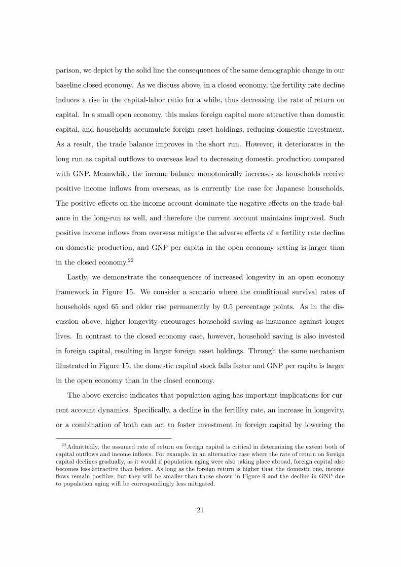
parison, we depict by the solid line the consequences of the same demographic change in our
baseline closed economy. As we discuss above, in a closed economy, the fertility rate decline
induces a rise in the capital-labor ratio for a while, thus decreasing the rate of return on
capital. In a small open economy, this makes foreign capital more attractive than domestic
capital, and households accumulate foreign asset holdings, reducing domestic investment.
As a result, the trade balance improves in the short run. However, it deteriorates in the
long run as capital out�ows to overseas lead to decreasing domestic production compared
with GNP. Meanwhile, the income balance monotonically increases as households receive
positive income in�ows from overseas, as is currently the case for Japanese households.
The positive e¤ects on the income account dominate the negative e¤ects on the trade bal-
ance in the long-run as well, and therefore the current account maintains improved. Such
positive income in�ows from overseas mitigate the adverse e¤ects of a fertility rate decline
on domestic production, and GNP per capita in the open economy setting is larger than
in the closed economy.22
Lastly, we demonstrate the consequences of increased longevity in an open economy
framework in Figure 15. We consider a scenario where the conditional survival rates of
households aged 65 and older rise permanently by 0.5 percentage points. As in the dis-
cussion above, higher longevity encourages household saving as insurance against longer
lives. In contrast to the closed economy case, however, household saving is also invested
in foreign capital, resulting in larger foreign asset holdings. Through the same mechanism
illustrated in Figure 15, the domestic capital stock falls faster and GNP per capita is larger
in the open economy than in the closed economy.
The above exercise indicates that population aging has important implications for cur-
rent account dynamics. Speci�cally, a decline in the fertility rate, an increase in longevity,
or a combination of both can act to foster investment in foreign capital by lowering the
22Admittedly, the assumed rate of return on foreign capital is critical in determining the extent both ofcapital out�ows and income in�ows. For example, in an alternative case where the rate of return on foreigncapital declines gradually, as it would if population aging were also taking place abroad, foreign capital alsobecomes less attractive than before. As long as the foreign return is higher than the domestic one, income�ows remain positive; but they will be smaller than those shown in Figure 9 and the decline in GNP dueto population aging will be correspondingly less mitigated.
21

return on domestic capital.23 In Figure 16, we chart the evolution of the current account
together with movements in population growth and average life span for the U.S., Japan,
and the average of advanced countries (AAC).24 The discrepancy between the current ac-
counts of the two countries was minimal around 1980, clearly widening subsequently. That
is, during the last two decades, Japan has maintained a current account surplus while the
U.S. has persistently experienced current account de�cits. As far as the two countries are
concerned, therefore, Japanese households invest in foreign capital and U.S. households
receive capital investment from overseas.
Turning our attention to demographic transitions, from the 1960s to the 1980s popula-
tion growth in the U.S., AAC, and Japan is seen to have evolved along similar trajectories.
This suggests that demographic change in this period would have had minimal e¤ects on
the current accounts of either the U.S. or Japan. Since the 1980s, however, the population
in the U.S. has grown quicker than in AAC, while in Japan it has grown more slowly.
Meanwhile, average life span in Japan has been longer than in the U.S. and AAC, where
it has evolved roughly in parallel. According to the simulations conducted above, these
demographic changes would have been expected to reduce the return on capital investment
in Japan relative to AAC, leading to capital �ow from Japan to AAC and a current account
surplus in Japan.25 An equivalent but opposite mechanism would have been expected to
operate for the U.S. What we see, therefore, is that the observed current account dynamics
and demographic changes in Japan and the U.S. during the last few decades are broadly
consistent with our model�s implications.
23Our result is consistent with the �ndings of Ferrero (2010), who evaluates the demographic e¤ects onU.S. current account developments, based on the life-cycle model of Gertler (1999).24See footnote to Table 1 for the de�nition of �more developed countries�.25Admittedly, our discussion here abstracts from the TFP movements considered key determinants of
current account dynamics in existing studies such as Ferrero (2010) and Chen et al. (2009). In thesestudies, a di¤erence in TFP growth rate between the two countries plays a dominant role in their currentaccount dynamics as it substantially a¤ects their respective returns to capital.
22

6 Conclusion
In this study, we quantitatively explore the macroeconomic impact of Japan�s population
aging using a full-�edged overlapping generations model. We calibrate the model to the
Japanese economy over the sample period 1982-2010. Under a set of plausible assumptions
about future paths of TFP as well as demographics, we make out-of-sample projections
for the next three decades. To gauge the impact of population aging on GNP and �scal
variables, we simulate our model under the counterfactual assumption in which population
aging is arrested. Since population aging in Japan is caused by both a decline in the fertility
rate and an increase in longevity, we evaluate these two e¤ects separately. We also examine
how in�uential public medical burdens are in impacting on GNP and �scal variables in the
aging Japan, by conducting a counterfactual experiment where a public health insurance
system is not explicitly incorporated as is the case with OG models commonly used in
previous studies.
We �nd that Japan�s population aging as a whole adversely a¤ects GNP growth by
dampening factor inputs. It also negatively impacts on GNP per capita and �scal variables,
especially in the future, mainly due to the decline in the fraction of the population of
working-age. For these �ndings, a decline in the fertility rate plays a quantitatively larger
role in lowering GNP growth and the primary balance to GNP ratio, because it reduces
the labor force population and the proportion of savers in the economy. Although working
households mitigate these adverse e¤ects by increasing their working hours and saving rates,
this is not enough to compensate for the e¤ects of the shrinking working-age population.
The e¤ects of increased longevity on economic growth are expansionary, but relatively
small. Our simulations predict that the negative e¤ects of fertility rate decline will expand
during the next few decades. We also �nd that public medical bene�ts partly �nanced by
payroll income tax have negative e¤ects on GNP per capita and the �scal balance. Our
results suggest that the impact of population aging is underestimated in previous studies
which assume that public medical bene�t is �nanced by lump-sum tax. Furthermore, in
a small open economy setting, we show that when domestic households have access to the
23

foreign asset market, they may mitigate the adverse e¤ects of population aging on GNP
by investing their savings in foreign capital with higher returns.
Our results imply that the ongoing and predicted demographic transition may be ex-
pected to have long-lasting adverse e¤ects on the Japanese economy. Our present analysis,
however, does not incorporate economic and institutional changes that may occur when a
society responds to population aging and that can potentially increase factor inputs; these
could include a higher female labor participation rate or social security reforms such as
postponing the retirement age. Extending the current model in these directions is left for
our future research.
24
A Construction of Exogenous Variables
This appendix documents the detailed de�nitions and construction methodologies for the
exogenous variables used in our baseline scenario simulation. The in-sample time series
of the variables fGt=Yt; � t=Yt; � c;t; �h;t; �k;t; �s;t; �m;t �t; f j;tg100j=21; �t; gtg2010t=1982 are
computed from the actual data, and the sequences of the two parameters f t; �tg2010t=1982 are
chosen so that the model-generated government bond yield and labor input capture the
actual counterparts successfully as described below. We make the following assumptions
about the out-of-sample time series of these variables.
� fGt=Yt; � t=Ytg1t=1982 :We construct the �government purchases to GNP ratio,�Gt=Yt;
from �gross �xed capital formation + government consumption expenditure - social
transfers in kind, payable,�divided by GNP, and the �transfers to GNP ratio,�� t=Yt;
from �other current transfers (receivable) - other current transfers (payable) + capital
transfers (receivable) - capital transfers (payable),�divided by GNP. For the purposes
of in-sample simulation, we construct the corresponding series using the actual data.
For the purposes of projection, we assume that the government purchases to GNP
ratio reverts linearly over the three decades from 2011 towards its historical average
and that the lump-sum transfers to GNP ratio stays constant at the steady state
level from 2011 onwards.
� f� c;tg1t=1982 : The consumption tax in the model is assumed to rise from zero to 3%
in 1989, and to 5% in 1997. For the forecast period, we assume that the consumption
tax rate is raised from 5% to 8% in 2014 and to 10% in 2015, unchanged thereafter.
� f�h;t; �k;tg1t=1982 : Closely following Hayashi and Prescott (2002), tax revenue from
capital income is calculated as �direct tax on �nancials + direct tax on non-�nancials +
.5 � indirect tax - .5 � value added taxes (VAT).�Tax revenue from labor income is
calculated as �direct tax on households + .5 � indirect tax - .5 � VAT.�Similarly,
capital income is constructed as �.5 � indirect tax - .5 � VAT + operating surplus in
corporate sector + operating surplus in housing non-corporate sector + .2� operating
25

surplus in non-housing non-corporate sector + net factor payments + adjustment for
statistical discrepancy.�Labor income is constructed as �.5 � indirect tax - .5 � VAT
+ compensation of employees + .8 � operating surplus in non-housing non-corporate
sector + adjustment for statistical discrepancy.�The tax rates are computed from the
tax revenues divided by the corresponding income. For out-of-sample projections, we
assume that over the three decades each tax rate linearly converges to its historical
average during 1982 to 2010.
� f�s;t; �m;tg1t=1982 : We assume that the coverage ratios of general government expen-
ditures/transfers to total public pension bene�ts and to total public medical bene�ts
are maintained at their 2010 levels (41.3% and 37.8%).26
� f�t; f j;tg100j=21g1t=1982 : The age-21 population growth rate is computed based on
the Annual Report on Current Population Estimate by the Statistics Bureau of the
Ministry of International A¤airs and Communication, for the sample period up until
2010. For the future horizon, these are computed based on the Projection of Future
Population by the National Institute of Population and Social Security Research
(IPSS). The age-speci�c conditional survival probabilities are computed from the
same data.
� fgt; �tg1t=1982 : The TFP growth rate up to 2010 is computed from the Solow residual
series, At = Yt=(Kat L
1�at ); that is constructed in line with Hayashi and Prescott
(2002) and ·Imrohoro¼glu and Sudo (2011a, b). For the periods beyond 2010, we
assume that the TFP growth rate is constantly 1%, which is the historical average of
the growth rate of the Solow residual from 1995 to 2007. The depreciation rate is set
to its actual value up to 2010, and linearly converges to 0.071, which is the historical
26We de�ne the public pension bene�ts as the sum of Welfare Pension, National Pension, Pensions ofSeamen�s Insurance, Long-term entitlements from the Federation of National Public Personnel Mutual AidAssociations, Long-term entitlements from the Pension Fund Association for Local Government O¢ cials,and Long-term entitlements from Others. We de�ne the public medical bene�ts as the sum of Health In-surance, Medical bene�ts of Seamen�s Insurance, National Health Insurance, the New Medical Care Systemfor the Elderly, Health insurance run by Private Mutual Associations, the Japan Health Insurance Associ-ation, Short-term entitlements from the Federation of National Public Personnel Mutual Aid Associations,Short-term entitlements from the Pension Fund Association for Local Government O¢ cials, and Short-termentitlements from Others.
26

average from 1982 to 2010, over the next three decades.
� f t; �tg1t=1982 : The utility weight on households�leisure is assumed to rise from unity
in 1988 to 1.37 in 1993 in a quadratic fashion, so as to incorporate the e¤ect of
institutional changes a¤ecting labor input into the model. As discussed by Hayashi
and Prescott (2002), a mandatory reduction of working hours was established in the
late 1980s, and the length of the working week drops from 44 hours in 1988 to 40 hours
in 1993.27 The in-sample sequence of utility weights on government bond holding is
set so that the model-generated government bond yield matches the corresponding
data series.28 The weight is set at the 2010 value in the forecast horizon.
B List of Equations
This appendix summarizes key equations used for computing transition equilibrium paths.
B.1 Demographic Structure
� Evolution of population:
P21;t = (1 + �t)P21;t�1: (B-1)
Pj;t = j;tPj�1;t�1 for j = 21; :::; 100: (B-2)
� Cohort share in total population:
�j;t =Pj;tP100i=21 Pi;t
for j = 21; :::; 100: (B-3)
27Based on a simple growth model, Hayashi and Prescott (2002) point out that the fall in workweeklength as well as the slowdown in TFP growth is important for the Japanese economic stagnation duringthe 1990s.28We construct the government bond yield series by dividing the nominal �net property income�of the
general government by the nominal �net �nancial liabilities�of the general government and the growth rateof the GNP de�ator.
27
B.2 Households�Optimality Conditions
� Budget constraints:
(1 + � c;t) cj;t + kj+1;t+1 + bj+1;t+1
=�1 + (1� �k;t) rKt
�kj;t + (1 + r
Bt )bj;t
+(1� �h;t) (1� � s;t � �m;t)wt"jhj;t + � t + �t for j � 65; (B-4)
(1 + � c;t) cj;t + kj+1;t+1 + bj+1;t+1
=�1 + (1� �k;t) rKt
�kj;t + (1 + r
Bt )bj;t + pbj;t + � t + �t for j > 65: (B-5)
� First order conditions with respect to consumption, labor input, capital and bond
holdings:(1 + � c;t+1) cj;t+1(1 + � c;t) cj;t
= � j+1;t+1�1 + (1� �k;t+1) rKt+1
�; (B-6)
t1� hj;t
=(1� � j;t) (1� � s;t � �m;t)wt"j
cj;t; (B-7)
�t1
bj;t+1+� j+1;t+1(1 + r
Bt+1)
(1 + � c;t+1) cj;t+1=
1
(1 + � c;t) cj;t; (B-8)
(1� �k;t)rKt � rBt =�t�1�(1 + � c;t)
100�1Xj=21
�j;tcj;t
bj+1;t+1: (B-9)
� Other conditions:
k21;t = b21;t = 0: (B-10)
k101;t = b101;t = 0: (B-11)
B.3 Firm�s Optimality Conditions
� Firm�s production of �nal goods with the Cobb-Douglas technology:
Yt = AtK�t L
1��t : (B-12)
� First order conditions with respect to capital demand and labor demand (real wage
28

and rental rates):
Rt = �At
�Kt
Lt
���1� rKt + �t; (B-13)
wt = (1� �)At�Kt
Lt
��: (B-14)
B.4 Social Security System
� Budget balance for public pension:
(1� �s;t)100X
j=65+1
Pj;tpbj;t = � s;twt
65Xj=21
Pj;t"jhj;t: (B-15)
� Budget balance for public health insurance:
(1� �m;t)100Xj=21
Pj;tmbj;t = �m;twt
65Xj=21
Pj;t"jhj;t: (B-16)
B.5 General Government
� Budget constraint:
(1 + rBt )Bt +Gt + �m;t
100Xj=21
Pj;tmbj;t + �s;t
100Xj=65+1
Pj;tpbj;t +
100Xj=21
Pj;t� t +
100Xj=21
Pj;t�t
= Bt+1 + � c;tCt + �h;t(1� � s;t � �m;t)wtLt + �k;trKt Kt: (B-17)
B.6 Market Clearing Conditions and Resource Constraint
� For capital, labor, government bonds, and �nal goods,
Kt =100Xj=21
Pj;tkj;t; (B-18)
Lt =65Xj=21
Pj;t"jhj;t; (B-19)
Bt =
100Xj=21
Pj;tbj;t; (B-20)
29
Yt = Ct +Kt+1 � (1� �t)Kt +Gt +100Xj=21
Pj;tmbj;t: (B-21)
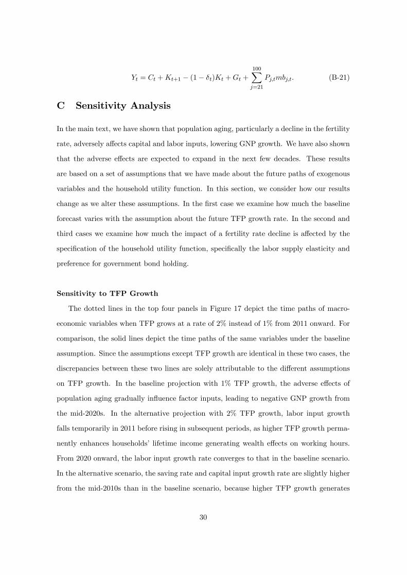
C Sensitivity Analysis
In the main text, we have shown that population aging, particularly a decline in the fertility
rate, adversely a¤ects capital and labor inputs, lowering GNP growth. We have also shown
that the adverse e¤ects are expected to expand in the next few decades. These results
are based on a set of assumptions that we have made about the future paths of exogenous
variables and the household utility function. In this section, we consider how our results
change as we alter these assumptions. In the �rst case we examine how much the baseline
forecast varies with the assumption about the future TFP growth rate. In the second and
third cases we examine how much the impact of a fertility rate decline is a¤ected by the
speci�cation of the household utility function, speci�cally the labor supply elasticity and
preference for government bond holding.
Sensitivity to TFP Growth
The dotted lines in the top four panels in Figure 17 depict the time paths of macro-
economic variables when TFP grows at a rate of 2% instead of 1% from 2011 onward. For
comparison, the solid lines depict the time paths of the same variables under the baseline
assumption. Since the assumptions except TFP growth are identical in these two cases, the
discrepancies between these two lines are solely attributable to the di¤erent assumptions
on TFP growth. In the baseline projection with 1% TFP growth, the adverse e¤ects of
population aging gradually in�uence factor inputs, leading to negative GNP growth from
the mid-2020s. In the alternative projection with 2% TFP growth, labor input growth
falls temporarily in 2011 before rising in subsequent periods, as higher TFP growth perma-
nently enhances households� lifetime income generating wealth e¤ects on working hours.
From 2020 onward, the labor input growth rate converges to that in the baseline scenario.
In the alternative scenario, the saving rate and capital input growth rate are slightly higher
from the mid-2010s than in the baseline scenario, because higher TFP growth generates
30

a higher return on capital, giving households an incentive to save more. However, these
e¤ects on GNP growth are quite limited. GNP growth in the alternative scenario is higher
than in the baseline scenario by approximately 1%. A positive growth rate is maintained
until 2040 in the alternative scenario, although it is dampened by population aging over
time.
Sensitivity to Labor Supply Elasticity
Second, we ask if the labor supply elasticity matters for the impact of population aging.
Existing studies, for example, Trabandt and Uhlig (2011) and ·Imrohoro¼glu and Kitao
(2009), investigate the importance of the size of the labor supply elasticity parameter for
the e¤ects of social security reforms or tax reforms within a general equilibrium framework.
Here we replace the functional form of the present utility function (8) with the following
utility function:
u (cj;t; 1� hj;t; bj+1;t+1) = log cj;t � th1+ 1
�j;t
1 + 1�
+ �t log bj+1;t+1 for j � 65;
where � is the Frisch elasticity of the labor supply. In general, � is supposed to be a positive
number less than unity.
In Case II of Figure 17 we compute the equilibrium paths of GNP per capita and
labor input growth under this alternative utility function with � = 0:5. The fertility rate
declines in the population aging scenario, but not in the alternative non-aging scenario.
Comparison with Figure 5 demonstrates how the speci�cation of the labor supply elasticity
a¤ects the impact from the fertility rate decline. With this speci�cation the variations in
labor input are less volatile in both the aging and non-aging scenarios than those in the
baseline scenario of Figure 5. However, the discrepancies between the two scenarios are
much the same as those observed in Figure 5. We can conclude that the macroeconomic
impact of declining fertility is not very sensitive to the elasticity of the labor supply.
31

Sensitivity to Utility from Government Bond Holding
Lastly, we ask if households�preference for government bond holding matters for the
impact of population aging. In our baseline simulation, we calibrate the utility weight
that households place on government bond holding �t so that the model-generated return
on government bonds rBt traces the data perfectly. Other things being equal, higher �t
implies a lower government bond yield, since households are willing to hold government
bonds even if the spread is wider. A lower government bond yield reduces government
interest repayments, moderating government bond accumulation through equation (24).
In Case III of Figure 17 we compute the equilibrium paths for the case where households
put a larger weight on government bond holding. Speci�cally from 2011 onward we set
the value of �t at double its value in the original speci�cation. Comparison with Figure 5
demonstrates how the speci�cation of households�utility preference for government bonds
a¤ects the impact of population aging. The discrepancies between the aging and non-aging
scenarios are not signi�cantly di¤erent from Figure 5. However, since households hold
government bonds at a low (or even negative) rate of return, the government bond yield
remains at lower levels under both the aging and non-aging scenarios.
32
References
[1] Arai, R., Ueda, J. (2012) �A Numerical Evaluation on a Sustainable Size of Primary
De�cit in Japan,�KIER Discussion Paper Series, 823.
[2] Auerbach, A., Kotliko¤, L. (1987) Dynamic Fiscal Policy, Cambridge University Press.
[3] Braun, R. A., Ikeda, D., Joines, D. H. (2009) �The Saving Rate in Japan: Why It Has
Fallen and Why It Will Remain Low,�International Economic review, 50, 291-321.
[4] Braun, R. A., Joines, D. H. (2012) �The Implications of a Greying Japan for Public
Policy,�mimeo.
[5] Chen, K., ·Imrohoro¼glu, A., ·Imrohoro¼glu, S. (2007) �The Japanese Saving Rate be-
tween 1960 and 2000: Productivity, Policy Changes, and Demographics,�Economic
Theory, 32, 87-104.
[6] Chen, K., ·Imrohoro¼glu, A., ·Imrohoro¼glu, S. (2009) �A quantitative assessment of the
decline in the U.S. current account,�Journal of Monetary Economics, 56, 1135-1147.
[7] Dekle, R. (2000) �Demographic density, per capita consumption, and the Japanese
saving-investment balance,�Oxford Review of Economic Policy, 16 (2), 46-60.
[8] Dekle, R. (2003) �Japan�s Fiscal Policy and Debt Sustainability,� in Structural Im-
pediments to Growth in Japan, Blomstrom et al. (eds.), University of Chicago Press.
[9] Ferrero, A. (2010) �A structural decomposition of the U.S. trade balance: Productiv-
ity, demographics and �scal policy,�Journal of Monetary Economics, 57(4), 478-490.
[10] Fujiki, H., Hirakata, N., Shioji, E. (2012) �Aging and Household Stock Hold-
ings: Evidence from Japanese Household Survey Data,� downloadable from
�http://www.imes.boj.or.jp/english/publication/conf/2012confsppa.html,� web-page
of the Institute for Monetary and Economic Studies, Bank of Japan.
[11] Hansen, G. D., ·Imrohoro¼glu, S. (2012) �Fiscal Reform and Government Debt in Japan:
A Neoclassical Perspective,�mimeo.
33
[12] Hayashi, F., Prescott, E. (2002) �The 1990s in Japan: A Lost Decade�, Review of
Economic Dynamics, 5, 206-235.
[13] Horioka, C. (1997) �A Cointegration Analysis of the Impact of the Age Structure of
the Population on the Household Saving Rate in Japan,�Review of Economics and
Statistics, 79, 511-516.
[14] Horioka, C., Watanabe, W. (1997) �Why Do People Save? A Micro-Analysis of Mo-
tives for Households Saving in Japan,�Economic Journal, 107, 537-552.
[15] Ihori, T., Kato, R., R., Kawade, M., Bessho, S. (2005) �Public Debt and Economic
Growth in an Aging Japan,�CARF F-Series CARF-F-046, Center for Advanced Re-
search in Finance, Faculty of Economics, The University of Tokyo.
[16] Ihori, T., Kato, R., R., Kawade, M., Bessho, S. (2011) �Health Insurance Reform and
Economic Growth: Simulation Analysis in Japan,� Japan and the World Economy,
23, 227-239.
[17] Ikeda, D., Saito, M. (2012) �The E¤ects of Demographic Changes on the Real Interest
Rate in Japan,�Bank of Japan Working Paper Series, 12-E-3.
[18] ·Imrohoro¼glu, S., Kitao, S. (2009) �Labor Supply Elasticity and Social Security Re-
form,�Journal of Public Economics, 93, 867-878.
[19] ·Imrohoro¼glu, S., Sudo, N. (2011a) �Productivity and Fiscal Policy in Japan: Short
Term Forecasts from the Standard Growth model,�Monetary and Economic Studies,
29, 73-106.
[20] ·Imrohoro¼glu, S., Sudo, N. (2011b) �Will a Growth Miracle Reduce Debt in Japan?�
IMES Discussion Paper Series, 2011-E-1, Bank of Japan.
[21] Koga, M. (2006) �The Decline of Japan�s Saving Rate and Demographic E¤ects,�
Japanese Economic Review, 2, 312-321.
[22] Kozu, T., Sato, Y., Inada, M. (2003) �Demographic Changes in Japan and their
Macroeconomic E¤ects,�Bank of Japan Working Paper Series, 04-E-6.
34

[23] Maddaloni, A., Musso, A., Rother, P., Ward-Warmedinger, M., Westermann, T.
(2006) �Macroeconomic implications of demographic developments in the euro area,�
European Central Bank Occasional Paper Series, 51.
[24] Miles, D. (1999) �Modelling the Impact of Demographic Change upon the Economy,�
Economic Journal, 109, 1-36.
[25] Oguro, K., Shimasawa, M. (2011) Matlab Niyoru Macro Keizai Model Nyuumon, Nip-
pon Hyouron-Sha.
[26] Trabandt, M., Uhlig, H. (2011) �The La¤er Curve Revisited,� Journal of Monetary
Economics, 58, 305-327.
35
1990 2010 2030
Canada 17 20 38
China 9 11 24
France 21 26 39
Germany 22 31 48
Italy 22 31 44
Japan 17 35 53
Russia 15 18 29
U.K. 24 25 34
U.S. 19 20 33
More Developed 19 24 36
Less Developed 8 9 15
(Source) United Nations, "World Population Prospects, the 2010 Revision."(Note) More developed regions comprise Europe, Northern America, Australia, New Zealand and Japan, and Less developed regions comprise all regions of Africa, Asia (excluding Japan), Latin America and the Caribbean plus Melanesia, Micronesia and Polynesia.
Table 1: Dependency Ratios
Dependency Ratio (over 65 age/15-64 age pop., %)
1985-90 2005-10 1990 2009
Canada 1.62 1.65 0.62 0.69
China 2.63 1.64 0.45 0.50
France 1.80 1.97 0.63 0.71
Germany 1.43 1.36 0.53 0.65
Italy 1.34 1.38 0.57 0.68
Japan 1.66 1.32 0.61 0.73
Russia 2.12 1.44 0.49 0.51
U.K. 1.84 1.83 0.57 0.65
U.S. 1.89 2.07 0.62 0.67
(Source) United Nations, "World Population Prospects, the 2010 Revision," World Health Organization, "Global Health Observatory Data Repository (Life Table)."(Note) Total fertility rate is defined as the number of children per woman.
Survival Rate of 85-89 age pop.Total Fertility Rate
Table 2: Total Fertility Rates and Elderly Survival Rates

0.406 0.972 0.30 Braun et al. (2009) NME (2009)
Table 3: Constant Parameters
Table 4: Steady State Values of Key Variables
G/Y B/Y /Y c h k s m g ρ
0.142 0.441 0.022 0.10 0.15 0.316 0.413 0.378 0.01 0.00
65
21j j
100
21j jmb

(1) Conditional Survival Probability
(2) Labor Efficiency
(3) Individual Medical Cost
Figure 1: Age-Specific Profiles
0.5
0.6
0.7
0.8
0.9
1.0
21 30 40 50 60 70 80 90 100
2040
2010
1982
(Index)
Yr YrYr
Age
0.5
0.6
0.7
0.8
0.9
1.0
1.1
1.2
1.3
21 25 30 35 40 45 50 55 60 65
(Index)
0.00
0.05
0.10
0.15
21 30 40 50 60 70 80 90 100
(Index)
Age
Age
(1) Growth Rate of TFP Factor (2) Fertility Rate (Age-21 Population Growth)
(3) Preference for Leisure (4) Government Purchases-GNP Ratio
(5) Current/Capital Transfers-GNP Ratio (6) Consumption Tax Rate
(7) Labor Income Tax Rate (8) Capital Income Tax Rate
(9) Coverage Ratios of General Government (10) Preference for Bond Holdings
(Note) Government purchases of (4) do not include public medical benefits.
Figure 2: Exogenous Time Series
0
2
4
6
8
10
8285 90 95 00 05 10 15 20 25 30 35 40
(%)
0
5
10
15
82 85 90 95 00 05 10 15 20 25 30 35 40
(%)
10
12
14
16
18
20
82 85 90 95 00 05 10 15 20 25 30 35 40
(%)
20
25
30
35
40
82 85 90 95 00 05 10 15 20 25 30 35 40
(%)
Yr
12
13
14
15
16
8285 90 95 00 05 10 15 20 25 30 35 40
(%)
10
20
30
40
50
82 85 90 95 00 05 10 15 20 25 30 35 40
Pension BenefitsMedical Benefits
(%)
-8-6-4-202468
82 85 90 95 00 05 10 15 20 25 30 35 40
(%)
0.8
1.0
1.2
1.4
1.6
82 85 90 95 00 05 10 15 20 25 30 35 40
(Index)
0.00
0.02
0.04
0.06
0.08
0.10
82 85 90 95 00 05 10 15 20 25 30 35 40
(Index)
-8-6-4-202468
8285 90 95 00 05 10 15 20 25 30 35 40
(%)
Yr
(1) Growth Rate of Real GNP (2) Real GNP per Capita
(3) Gross National Saving Rate (4) After-Tax Rate of Return on Capital
(5) Capital-Labor Ratio (6) Capital Share of Total Assets
(7) Pension Benefits-GNP Ratio (8) Medical Benefits-GNP Ratio
(9) Primary Balance-GNP Ratio (10) Net Government Debt-GNP Ratio
Figure 3: Model Performance
14 16 18 20 22 24 26 28 30 32 34
82 85 90 95 00 05 10
4
5
6
7
8
9
82 85 90 95 00 05 10
(%)(%)
-10 -8 -6 -4 -2 0 2 4 6 8
10
82 85 90 95 00 05 10
Data Model
Yr
(%)
3
6
9
12
82 85 90 95 00 05 10
(%)
2
4
6
8
82 85 90 95 00 05 10
(%)
0.7
0.8
0.9
1.0
1.1
82 85 90 95 00 05 10
(Index: Normalized to unity in 2000)
-12 -10
-8 -6 -4 -2 0 2 4 6
82 85 90 95 00 05 10
(%)
0
20
40
60
80
100
120
140
82 85 90 95 00 05 10
(%)
3
4
5
6
7
8
9
82 85 90 95 00 05 10
(Index)
70
80
90
100
82 85 90 95 00 05 10
(%)
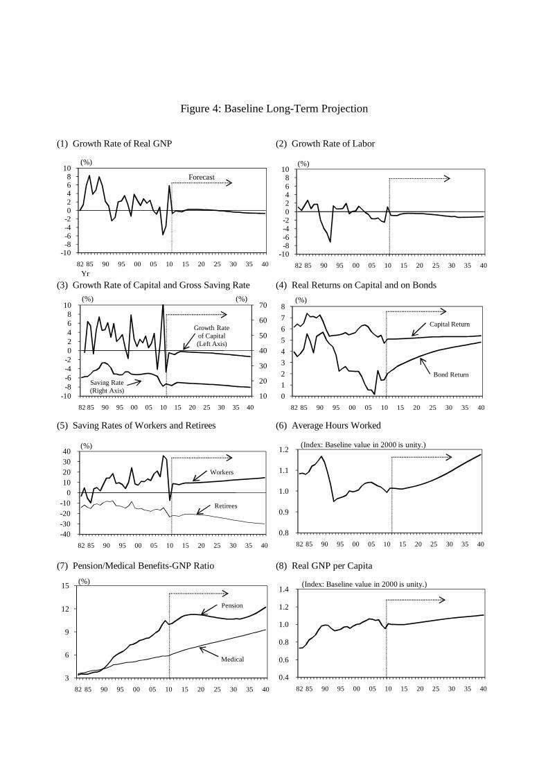
(1) Growth Rate of Real GNP (2) Growth Rate of Labor
(3) Growth Rate of Capital and Gross Saving Rate (4) Real Returns on Capital and on Bonds
(5) Saving Rates of Workers and Retirees (6) Average Hours Worked
(7) Pension/Medical Benefits-GNP Ratio (8) Real GNP per Capita
Figure 4: Baseline Long-Term Projection
10
20
30
40
50
60
70
-10 -8 -6 -4 -2 0 2 4 6 8
10
82 85 90 95 00 05 10 15 20 25 30 35 40
Growth Rate of Capital (Left Axis)
Saving Rate(Right Axis)
0
1
2
3
4
5
6
7
8
82 85 90 95 00 05 10 15 20 25 30 35 40
Bond Return
Capital Return
(%) (%)
-10-8-6-4-202468
10
82 85 90 95 00 05 10 15 20 25 30 35 40
(%)
Forecast
-40 -30 -20 -10
0 10 20 30 40
82 85 90 95 00 05 10 15 20 25 30 35 40
(%)
Workers
Retirees
-10-8-6-4-202468
10
82 85 90 95 00 05 10 15 20 25 30 35 40
(%)
Yr
(%)
0.8
0.9
1.0
1.1
1.2
82 85 90 95 00 05 10 15 20 25 30 35 40
(Index: Baseline value in 2000 is unity.)
0.4
0.6
0.8
1.0
1.2
1.4
82 85 90 95 00 05 10 15 20 25 30 35 40
(Index: Baseline value in 2000 is unity.)
3
6
9
12
15
82 85 90 95 00 05 10 15 20 25 30 35 40
(%)
Pension
Medical

(1) Growth Rate of Real GNP (2) Growth Rate of Labor
(3) Growth Rate of Capital and Gross Saving Rate (4) Real Returns on Capital and on Bonds
(5) Saving Rates of Workers and Retirees (6) Average Hours Worked
(7) Pension/Medical Benefits-GNP Ratio (8) Real GNP per Capita
Figure 5: Impact of Decline in Fertility Rate (Counterfactual Simulation)
0
1
2
3
4
5
6
7
8
82 85 90 95 00 05 10 15 20 25 30 35 40
Bond Return
[Assumption] No fertility rate decline: the size of the age-21 population is held constant from 1995. Other exogenous series are identical to Figure 4.
(%)
-10-8-6-4-202468
10
82 85 90 95 00 05 10 15 20 25 30 35 40
BaselineSimulation
(%)
Impacts of Decline in Fertility Rate
-40 -30
-20
-10 0
10
20 30
40
82 85 90 95 00 05 10 15 20 25 30 35 40
(%)
Workers
Retirees
-10-8-6-4-202468
10
82 85 90 95 00 05 10 15 20 25 30 35 40
(%)
Capital Return
10
20
30
40
50
60
70
-10 -8 -6 -4 -2 0 2 4 6 8
10
82 85 90 95 00 05 10 15 20 25 30 35 40
(%)
Growth Rate of Capital
(Left Axis)
Saving Rate(Right Axis)
(%)
Yr
0.8
0.9
1.0
1.1
1.2
82 85 90 95 00 05 10 15 20 25 30 35 40
(Index: Baseline value in 2000 is unity.)
3
6
9
12
15
82 85 90 95 00 05 10 15 20 25 30 35 40
(%)
Pension
Medical0.4
0.6
0.8
1.0
1.2
1.4
82 85 90 95 00 05 10 15 20 25 30 35 40
(Index: Baseline value in 2000 is unity.)

(1) Primary Balance-GNP Ratio (2) Net Government Debt
Figure 6: Impact of Decline in Fertility Rate on Real GNP per Capita
Figure 7: Impact of Decline in Fertility Rate on Fiscal Balance
-20
-15
-10
-5
0
5
10
15
20
82 85 90 95 00 05 10 15 20 25 30 35 40
Real GNP per worker
Fraction of worker
Real GNP per capita
(Discrepancy between the two scenarios, %)
Yr
-6
-5
-4
-3
-2
-1
0
1
8285 90 95 00 05 10 15 20 25 30 35 40
(Discrepancy from the baseline, % points)
-10
0
10
20
30
40
8285 90 95 00 05 10 15 20 25 30 35 40
(Discrepancy from the baseline, %)
Yr
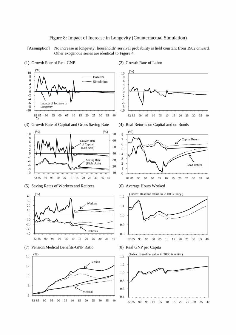
(1) Growth Rate of Real GNP (2) Growth Rate of Labor
(3) Growth Rate of Capital and Gross Saving Rate (4) Real Returns on Capital and on Bonds
(5) Saving Rates of Workers and Retirees (6) Average Hours Worked
(7) Pension/Medical Benefits-GNP Ratio (8) Real GNP per Capita
Figure 8: Impact of Increase in Longevity (Counterfactual Simulation)
10
20
30
40
50
60
70
-10 -8 -6 -4 -2 0 2 4 6 8
10
82 85 90 95 00 05 10 15 20 25 30 35 40
(%) (%)
Growth Rate of Capital(Left Axis)
Saving Rate (Right Axis)
0
1
2
3
4
5
6
7
8
82 85 90 95 00 05 10 15 20 25 30 35 40
Capital Return
[Assumption] No increase in longevity: households' survival probability is held constant from 1982 onward.Other exogenous series are identical to Figure 4.
(%)
-10 -8 -6 -4 -2 0 2 4 6 8
10
82 85 90 95 00 05 10 15 20 25 30 35 40
BaselineSimulation
(%)
Impacts of Increase in Longevity
-40 -30 -20 -10
0 10 20 30
40
82 85 90 95 00 05 10 15 20 25 30 35 40
(%)
Workers
Retirees
-10 -8 -6 -4 -2 0 2 4 6 8
10
82 85 90 95 00 05 10 15 20 25 30 35 40
(%)
Bond Return
Yr
0.8
0.9
1.0
1.1
1.2
82 85 90 95 00 05 10 15 20 25 30 35 40
(Index: Baseline value in 2000 is unity.)
3
6
9
12
15
82 85 90 95 00 05 10 15 20 25 30 35 40
(%)
Pension
Medical
0.4
0.6
0.8
1.0
1.2
1.4
82 85 90 95 00 05 10 15 20 25 30 35 40
(Index: Baseline value in 2000 is unity.)

(1) Primary Balance-GNP Ratio (2) Net Government Debt
Figure 9: Impact of Increase in Longevity on Real GNP per Capita
Figure 10: Impact of Increase in Longevity on Fiscal Balance
-20
-15
-10
-5
0
5
10
15
20
82 85 90 95 00 05 10 15 20 25 30 35 40
Real GNP per worker
Fraction of worker
Real GNP per capita
(Discrepancy between the two scenarios, %)
Yr
-6
-5
-4
-3
-2
-1
0
1
8285 90 95 00 05 10 15 20 25 30 35 40
(Discrepancy from the baseline, % points)
-10
0
10
20
30
40
8285 90 95 00 05 10 15 20 25 30 35 40
(Discrepancy from the baseline, %)
Yr

(1) Growth Rate of Real GNP (2) Growth Rate of Labor
(3) Growth Rate of Capital and Gross Saving Rate (4) Real Returns on Capital and on Bonds
(5) Saving Rates of Workers and Retirees (6) Average Hours Worked
(7) Pension/Medical Benefits-GNP Ratio (8) Real GNP per Capita
Figure 11: Impact of Public Medical Benefit (Counterfactual Simulation)
10
20
30
40
50
60
70
-10 -8 -6 -4 -2 0 2 4 6 8
10
82 85 90 95 00 05 10 15 20 25 30 35 40
(%) (%)
Growth Rate of Capital(Left Axis)
Saving Rate (Right Axis)
-3 -2 -1 0 1 2 3 4 5 6 7 8
82 85 90 95 00 05 10 15 20 25 30 35 40
Capital Return
[Assumption] Part of public medical benefit is financed by lump-sum tax on all living households, instead of payroll income tax on working households. Other exogenous series are the same as in Figure 4.
(%)
-3
-2
-1
0
1
2
3
82 85 90 95 00 05 10 15 20 25 30 35 40
BaselineSimulation
(%)
Impacts of Public Health Insurance System
-40 -30 -20 -10
0 10 20 30
40
82 85 90 95 00 05 10 15 20 25 30 35 40
(%)
Workers
Retirees
-3
-2
-1
0
1
2
3
82 85 90 95 00 05 10 15 20 25 30 35 40
(%)
Bond Return
Yr
0.8
0.9
1.0
1.1
1.2
82 85 90 95 00 05 10 15 20 25 30 35 40
(Index: Baseline value in 2000 is unity.)
3
6
9
12
15
82 85 90 95 00 05 10 15 20 25 30 35 40
(%)
Pension
Medical
0.4
0.6
0.8
1.0
1.2
1.4
82 85 90 95 00 05 10 15 20 25 30 35 40
(Index: Baseline value in 2000 is unity.)
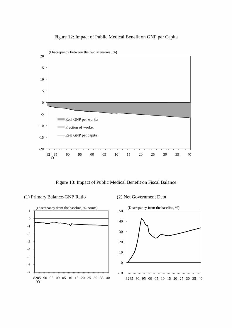
(1) Primary Balance-GNP Ratio (2) Net Government Debt
Figure 12: Impact of Public Medical Benefit on GNP per Capita
Figure 13: Impact of Public Medical Benefit on Fiscal Balance
-20
-15
-10
-5
0
5
10
15
20
82 85 90 95 00 05 10 15 20 25 30 35 40
Real GNP per worker
Fraction of worker
Real GNP per capita
(Discrepancy between the two scenarios, %)
Yr
-7
-6
-5
-4
-3
-2
-1
0
1
8285 90 95 00 05 10 15 20 25 30 35 40
(Discrepancy from the baseline, % points)
-10
0
10
20
30
40
50
8285 90 95 00 05 10 15 20 25 30 35 40
(Discrepancy from the baseline, %)
Yr

(1) Return on Capital (2) Growth Rate of Real GNP
(3) Saving Rate (4) Investment Rate
(5) Current Account-GNP Ratio (6) Trade Balance-GNP Ratio
(7) Income Account-GNP Ratio (8) Real GNP per Capita
Figure 14: Impact of Decline in Fertility Rate on Current Account
-6
-4
-2
0
2
4
6
1 10 20 30 40
(Discrepancy from the baseline, % points)
-6
-4
-2
0
2
4
6
1 10 20 30 40
(Discrepancy from the baseline, % points)
-6
-4
-2
0
2
4
6
1 10 20 30 40
(Discrepancy from the baseline, % points)
[Assumption] The growth rate of age-21 population declines permanently by 1.0% point. Domestic return on capital is equalized to foreign return on capital.
-0.3
-0.2
-0.1
0.0
0.1
0.2
0.3
1 10 20 30 40
Closed
Small Open
(Discrepancy from the baseline, % points)
Period
-1.0
-0.5
0.0
0.5
1.0
1 10 20 30 40
(Discrepancy from the baseline, % points)
-6
-4
-2
0
2
4
6
1 10 20 30 40
(Discrepancy from the baseline, % points)
-6
-4
-2
0
2
4
6
1 10 20 30 40
(Discrepancy from the baseline, % points)
-3
-2
-1
0
1
2
3
1 10 20 30 40
(Discrepancy from the baseline, %)

(1) Return on Capital (2) Growth Rate of Real GNP
(3) Saving Rate (4) Investment Rate
(5) Current Account-GNP Ratio (6) Trade Balance-GNP Ratio
(7) Income Account-GNP Ratio (8) Real GNP per Capita
Figure 15: Impact of Increase in Longevity on Current Account
-3
-2
-1
0
1
2
3
1 10 20 30 40
(Discrepancy from the baseline, % points)
-3
-2
-1
0
1
2
3
1 10 20 30 40
(Discrepancy from the baseline, % points)
-3
-2
-1
0
1
2
3
1 10 20 30 40
(Discrepancy from the baseline, % points)
[Assumption] The conditional survival probabilities of age 65 over households rise permanently by 1.0% point. Domestic return on capital is equalized to foreign return on capital.
-0.3
-0.2
-0.1
0.0
0.1
0.2
0.3
1 10 20 30 40
Closed
Small Open
(Discrepancy from the baseline, % points)
Period
-1.0
-0.5
0.0
0.5
1.0
1 10 20 30 40
(Discrepancy from the baseline, % points)
-3
-2
-1
0
1
2
3
1 10 20 30 40
(Discrepancy from the baseline, % points)
-3
-2
-1
0
1
2
3
1 10 20 30 40
(Discrepancy from the baseline, % points)
-3
-2
-1
0
1
2
3
1 10 20 30 40
(Discrepancy from the baseline, %)

(1) Current Account (to GDP Ratio)
(2) Population Growth Rate
(3) Average Life Span
(Source) IMF "World Economic Outlook," United Nations "World Population Prospects (Medium Forecast),"(Source) Japanese Cabinet Office "National Accounts," U.S. Department of Commerce "National Income and(Source) Product Accounts."(Note) 'Average of Advanced Countries' corresponds to the category 'More Developed Regions' by United (Note) Nations "World Population Prospects (Medium Forecast)."
Figure 16: Current Account and Demographics in Japan and the U.S.
-8
-6
-4
-2
0
2
4
6
8
1960 1965 1970 1975 1980 1985 1990 1995 2000 2005 2010 2015
Japan U.S.
(%)
Yr
Forecastby IMF
-4
-2
0
2
4
6
8
10
1960 1970 1980 1990 2000 2010 2020 2030 2040 2050
Japan
U.S.
Average of Advanced Countries
(%)
Yr
Forecast by UN
65
70
75
80
85
90
1955-1960 1965-1970 1975-1980 1985-1990 1995-2000 2005-2010 2015-2020 2025-2030 2035-2040 2045-2050
(Age)
Yr
Forecast by UN
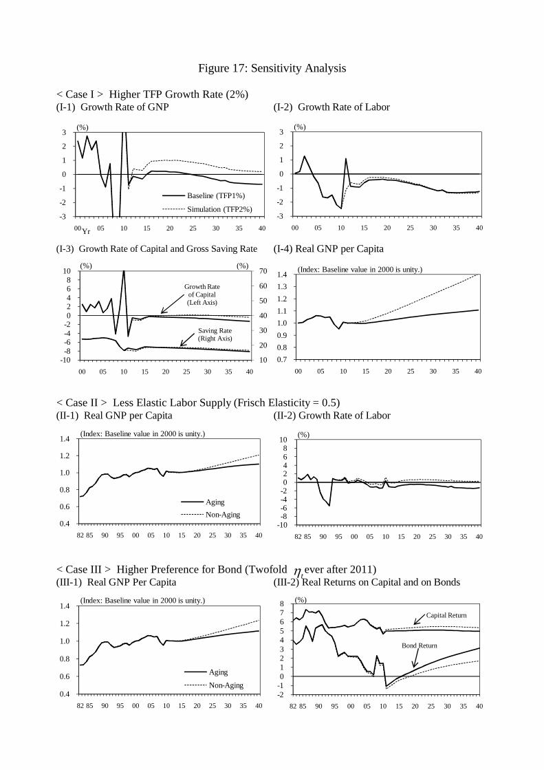
< Case I > Higher TFP Growth Rate (2%)(I-1) Growth Rate of GNP (I-2) Growth Rate of Labor
(I-3) Growth Rate of Capital and Gross Saving Rate (I-4) Real GNP per Capita
< Case II > Less Elastic Labor Supply (Frisch Elasticity = 0.5)(II-1) Real GNP per Capita (II-2) Growth Rate of Labor
< Case III > Higher Preference for Bond (Twofold ever after 2011)(III-1) Real GNP Per Capita (III-2) Real Returns on Capital and on Bonds
Figure 17: Sensitivity Analysis
10
20
30
40
50
60
70
-10 -8 -6 -4 -2 0 2 4 6 8
10
00 05 10 15 20 25 30 35 40
(%) (%)
Growth Rate of Capital(Left Axis)
Saving Rate (Right Axis)
-3
-2
-1
0
1
2
3
00 05 10 15 20 25 30 35 40
(%)
0.7
0.8
0.9
1.0
1.1
1.2
1.3
1.4
00 05 10 15 20 25 30 35 40
(Index: Baseline value in 2000 is unity.)
-3
-2
-1
0
1
2
3
00 05 10 15 20 25 30 35 40
Baseline (TFP1%)
Simulation (TFP2%)
(%)
Yr
0.4
0.6
0.8
1.0
1.2
1.4
82 85 90 95 00 05 10 15 20 25 30 35 40
Aging
Non-Aging
(Index: Baseline value in 2000 is unity.)
-10 -8 -6 -4 -2 0 2 4 6 8
10
82 85 90 95 00 05 10 15 20 25 30 35 40
(%)
0.4
0.6
0.8
1.0
1.2
1.4
82 85 90 95 00 05 10 15 20 25 30 35 40
Aging
Non-Aging
(Index: Baseline value in 2000 is unity.)
-2 -1 0 1 2 3 4 5 6 7 8
82 85 90 95 00 05 10 15 20 25 30 35 40
Capital Return
(%)
Bond Return
t


![Aging population and real exchange rate appreciation: the ...faculty.arts.ubc.ca/kgente/RERjap03044[1].pdf · Aging population and real exchange rate appreciation: the case of Japan](https://cdn.vdocuments.us/doc/165x107/5cbcfbe288c9936c1b8b746e/aging-population-and-real-exchange-rate-appreciation-the-1pdf-aging-population.jpg)


