1
Macroeconomic Environment and Financial Sector’s Performance: Econometric Evidence from Three Traditional Approaches
Muhammad Shahbaz∗, S.M.Aamir Shamim** and Naveed Aamir***
Abstract: The stable macroeconomic conditions are the prerequisites for sound and healthy
performance of the financial sector in the country. This study explores the impact of
macroeconomic environment on financial sector’s performance in Pakistan.
Present paper reveals that previous policies of financial institutions and economic growth
have improved the level of financial development. Both increase in government spending
as well as foreign remittances pushes the performance of financial sector in the upward
direction. Contrarily, the efficiency of financial markets deteriorates on account of rising
inflation due to its damaging impact while literacy rate is having negative influence on
banking sector in Pakistan. Trade openness along with improved capital inflows opens
new directions to improve the development of financial markets in the country. Further
more, performance of financial sector is attached with qualified institutions. High savings
rate declines the efficiency of banking sector and political instability retards the
performance of financial markets.
Key Words: Financial Development, Macroeconomic Environment, Cointegration
JEL Classification: F36, B22, C4
Note: Views are own of authors not representing SPDC.
Introduction An effective and efficient functioning of the financial sector requires sound and favorable
macroeconomic environment in the country. However, in this era of globalization it is
imperative for the financial sector to be strongly integrated in the global economy. In
∗ M.phill student at National College of Business Administration and Economics at Lahore, Pakistan ** SEVP at Dawood Islamic Bank Ltd. Karachi, Pakistan. *** Economist at Social Policy and Development Centre - Karachi, Pakistan
2
Pakistan, although, financial markets have been liberalized and operating on competitive
basis but still has to go a long way to achieve the required level of development. One may
conclude that the process of liberalization created a mushroom growth of both the non-
banking financial institutions (NBFIs) and banks, giving rise to profit competition and
also their existence. Infact, during the past few years, a major chunk of the financial
sector has been shifted from the public sector towards the private ownership in the
country1. In Pakistan, financial soundness indicators (FSIs) reflect an upward moving
trend but there are weaknesses and gaps which demand certain reforms specially the
under-developed legal system23.
Macroeconomic condition which determines the level of credit worthiness of the
borrowers, asset quality, increase and decrease in the value of collateral, etc are the main
sources of macro-economic shocks to the bank’s portfolio. Furthermore, regulatory
environment of an economy, level of financial development and level of concentration of
the financial sector also explains it’s performance. The instruments of monetary policy
like inflation, real exchange rate, short-term interest rate work as important determinants
of FSIs. According to Sundararajan et.al., (2002), FSIs can capture a range of factors
which impose risks to the financial system. So, for long term sustainability of the
financial sector, banks should be capable to operate in a competitive environment while
mitigating the risk factor.
1 The benefits of financial liberalization, as mentioned by Martell and Stultz, (2003) can only be achieved if the system develops to a level that the entire process of liberalization become deep rooted inside the financial sector institutions. Important FSIs consists of capital adequacy, asset quality and profitability which clearly reflects the performance of the banking sector Podpiera (2004). 2 Infact, the size of the impact on capital adequacy clearly indicates the sector’s vulnerability regarding credit risk. According to Stulz (1999), this financial globalization reduce the cost of capital equity on account of the decrease in expected returns to compensate risk. 3 Considering the risks to the banking sector soundness, increased government intervention is a strong element in enhancing this risk. This involves strict government policies with regard to credit requirements, interest rates and the overall functioning of the banking sector without taking into account the overall market forces creating high lending risks for the sector at large. But, in case of lending to the public sector La Porta and others, 2002, explained that although it is profitable but highly inefficient for the banking sector as banks earn easy profits, engage in little client competition, etc. This impact of public sector borrowing is also harmful in the long run for the banking sector liquidity as it absorbs substantial credit and effect their structural characteristics while crowding out the private sector credit. Specially, inefficient banks of the developing economies often adopt this strategy to earn profits while neglecting the efficiency of the financial sector and harm the overall financial deepening process.
3
As mentioned earlier, financial liberalization leads to development of financial market as
more funds are available in the market on reduced rates. As Claessens et al. (2002) and
Levine and Schmukler (2003) pointed out that a shift from domestic towards international
markets provides firms to acquire benefits on account of international portfolio
diversification. Therefore, removing capital controls provide more productive investment
opportunities. The real effects of financial and trade openness can be seen with an
increased trading in the stock market. Well developed stock markets along with the
developed banking system together raises economic wealth of the country (Rajan and
Zingales, 2003). Financial development and trade openness appears to have a positive
relationship in countries which are open to capital flows, (Rajan and Zingales 2003,
Huang and Temple 2005. Trade openness increases the size of capital markets for both
equity and debt finance.
The development of the equity market which is expected after capital account
liberalization can only be achieved if the legal and institutional development has reached
at the desired level. Capital account liberalization is a prerequisite for liberalization of
cross-border transaction of goods as indicated by Aizenman and Noy (2004). Whereas,
the development of equity market can only be possible if the banking sector is well
developed. Sometimes the growth of equity market in comparison to the size of the
market is related with the periods of economic crises and that point of time policy makers
suggest reduction in the level of financial openness (Ito, 2004). In short, financial
liberalization is beneficial in an environment of strong legal and institutional
infrastructure of the financial sector4.
4 During the period of economic downturns, countries with less developed financial system and lower levels of income provide higher capital ratios as noted by Whong, Choi and Fong (2005). This indicates to the fact that when economy is towards downward trend the quality of it’s assets deteriorate. In addition, higher inflation, unemployment and interest rates all worsens asset quality thereby increasing the non-performing loans. Banks are then forced to undertake risk on their capital which then gives high returns. Loan provisioning highlights the necessity of credit expansion in order to reduce the pressure of non-performing loans. Normally there is a lag effect of non-performing loans and banks create cushion for it during the period of credit expansion which also secure them sin case of economic downturn.

4
Body, et al. (1996), and Azariadis and Smith (1996), argued that, if inflation is high
enough, returns on savings are reduced which leads to a reduction in savings and savers.
Similarly, the pool of borrowers is swamped, informational frictions become more severe
and therefore credit becomes scarce in such an economy5. Furthermore, these economies
obviously present less efficient financial markets because of the higher interest rates that
follow high rates of inflation (Bittencourt, 2006). On the empirical surface, Haslag and
Koo (1999), and Boyd, Levine, et al. (2001), reported that moderate inflation has a
negative impact on financial development, as theoretically predicted. Moreover, both
studies find evidence of nonlinearities, i.e. after a particular threshold–15 percent per year
in Boyd, Levine, et al. (2001)–inflation presents only smaller marginal negative effects
on financial sector development. The intuition, not backed by theory though, is that the
damage on finance is done at rates of inflation lower than the proposed threshold
(Bittencourt, 2007). The recent case-study on Brazil by Bittencourt, (2007) & Shahbaz,
et, al (2007) for Pakistan; basing on time-series data, suggested that high rate of inflation
presented deleterious effects on finance6.
Haung and Temple analyzed that openness is more linked with bank-based finance as
compared with the stock market development, while further explaining that openness to
trade and finance are strongly correlated for higher-income countries, but not for lower-
income. In fact, trade provides benefits through specialization and scale of economies. A
much more complex situation arise when trade increase productivity and living standards
especially in the case if trade openness serves to promote financial development in the
country. Trade openness may be linked with high risks, including exposure to external
shocks and foreign competition7 as pointed out by Svaleryd and Vlachos (2000). This
will encourage the development of financial markets that can be used to diversify these
5 On a slightly dissimilar thread, Schreft and Smith (1997), Boyd and Smith (1996), Huybens and Smith (1998), and Huybens and Smith (1999), explored the new side that economies with higher rates of inflation do not approach or reach the steady state point where their capital stocks are high, i.e. there are bifurcations and development traps arise in such economies. 6 When inflation is very low, credit market frictions may be “non-binding,” so that inflation does not distort the flow of information or interfere with resource allocation and growth. However, once the rate of inflation exceeds some threshold level, credit market frictions become binding, and there is a discrete drop in financial sector performance as credit rationing intensifies (Boyd et, al, 2001). 7 Svalery and Vlachos (2002) also found positive association between financial development and liberal trade policies.

5
risks, and also help firms to overcome short run adverse shocks [Beck, (2002), and,
Svaleryd and Vlachos,(2000)]8. A robust link between openness and share of investment
in the GDP is confirmed by Levine and Renelt (1992), infact this could promote financial
development if high investment economies are trading economies. Moreover, the
development of equity market also takes place when there is financial opening and
succeeding trade opening especially in an economy where there is a well developed legal
system. Trade openness is a necessary condition for financial opening. Thus, due to the
nature of specialization and sectoral structure, the demand for external finance is
influenced by trade openness or through the innovation and technology transfer which
requires intensive use of external finance.
A formal model used by Alessandria and Qian (2005) indicate that capital account
liberalization has ambiguous effects on the efficiency of domestic financial
intermediaries. Aizenman and Noy (2003), Aizenman (2004) and, Chin and Ito (2005)
suggest that capital account liberalization is often preceded by goods market openness
because trade integration makes restrictions on capital flows which appears difficult to
sustain. Thus, increased openness in goods transactions leads to increased openness in the
capital account which is crucial for financial development, whereas the reverse situation
does not exist. In short, financial development on account of financial opening guided by
trade opening only occurs when the level of legal and institutional development is
efficiently administered.
Current literature strongly emphasize on the linkages between institutions and trade
openness, specially (Becker and Greenberg, 2004) highlights the very fact that how the
quality of institutions may affect comparative advantage and international specialization.
In this connection that how institutions generate comparative advantage Levchenko
(2003) provides model while explaining that the net exports in industries depending on
external finance are higher in countries with good finance9. Whereas, another work by
8 Using stock market for emerging economies, Li. et. al., (2004) find that goods markets openness is associated with greater market wide variations, but not greater firm-specific variations. 9 Vlachos and Svaleryd use the industry measure introduced by Rajan and Zingales, which was initially shown to capture how much an industry’s growth rate depends on financially development. Hence, Vlachos
6
Grossman and Helpman (2004) show that how institutional problems limit the amount of
outsourcing to low-wage countries. Many authors like Coeffee, (2000); La Porta. et.al,
(1990); Rajan and Zingales, (1998); Stulz and Williamson, (2001) discussed the channel
through which a country’s institutional inheritance affects financial sector development.
The emphasis of empirical analysis to the settler mortality hypothesis has been further
explained by Beck et, al., (2003) in which he indicates that the cross-variation in financial
intermediary and stock market capitalization has been better explained by the initial
endowments hypothesis Beck. et. al., (2003) do not investigate any of the intermediate
linkages rather emphasize more on the historical determinants of financial development.
The relationship between initial endowments and subsequent financial development, for
instance, might reflect factors which are important for financial development rather than
those focusing towards the development of institutions.
Further, explaining those factors which influence financial development, a study by Law
and Demetriades (2005), indicates that simultaneous openness to both trade and capital
inflows has a positive influence on financial development, in tandem with [institutions]
hypothesis, while the quality of country’s institutions has a separate influence on
financial development10. Basically, economic development is effected by capital account
liberalization through the process of financial development. It is often observed that
financially liberalized markets have a positive impact on the development of financial
markets. These developed financial markets play a major role as they are the main source
of funding for the borrowers in case of productive investment opportunities. Capital
account liberalization helps in developing the financial system in several ways. Quite
often, the cost of equity capital is reduced on account of financial liberalization or
because of the process of financial globalization and this provides easy access to the
borrowers. This situation emerges on account of lower expected returns, which generally
compensate for the risk. Then the inefficient financial institutions no longer exist in this
and Svaleryd essentially establish that some of the faster growth in finance-dependant industries located in financially well-developed countries actually results in higher exports (rather than domestic consumption). 10 Svaleryd and Vlachos (2000) suggest that development of institutions is necessary for risk diversifications, e.g. financial markets, mitigate to reduce barriers to trade. In contrast, Roderick (1999) provides evidence that openness to trade also increases the permanent degree of income volatility in an economy.
7
process of liberalization, thereby, demanding overall reforms of the financial
infrastructure. Eventually, an efficient financial system emerges with increased credit
availability in the market.
The role of financial system is not only to transform risk and acquire productive
investment opportunities at a low cost but also to operate as a transfer mechanism for
savings to be moved from those with surplus towards those in need. According to Levine
(1997) saving mobilization is one of the key functions of the financial sector – an
important determinant of economic growth. In the presence of under developed financial
system these private savings are used for housing and other domestic needs while
reducing the overall national saving rate. But a widespread deep financial system through
introduction of various schemes like superannuation can result in increased sustainable
national savings. On the contrary, benefits of sustained level of national savings results in
the form of developed financial system with positive effects on growth and productivity
in the economy.
Another important component for economic and financial development is the overall
stability in the country which is also conducive for human development. The movement
or the flow of remittances and savings towards financial institutions and use for human
capital formation all require stable environment. Benhabib and Spiegel (1994) propose a
measure of human capital accumulation (HCA) to examine cross-country evidence of
physical and human capital stocks on the determinants of the capacity of nations to adopt,
implement and innovate new technologies. Improvement in the indicators of health,
education and general standard of living explains the extent of human development in
any country. But a country with weak political and financial environment cannot benefit
an individual or the society from the growing trends of globalization.
Thus, changes in technology (Bulter and Merton, 1992), non-financial sector policies like
fiscal policies (Bencivenga and Smith, 1991), the legal system (Laporta et al., 1996),
political changes and human resources development, impact on the relationship between
financial development and economic development. Although, it is difficult to explain the
8
socio-political instability, but it can be used for econometric analysis as explained by
Venieris and Gupta, 1986. In-fact the traditional model of economic growth is changed
by incorporating particularly the factors of political violence and socio-political variables
in general as indicated by Gupta (1990). Socio-political instability introduces a new
element of uncertainty in the decision making process, as shown by Venieris and Gupta
(1986). In the absence of social political stability in the economy, development of
financial institutions gets restricted and its effects are not conducive for individual or
institutions. Trends in our financial system, the effects of regulatory settings on our
capital markets access to finance, the process of decision making, etc, all requires social
political stability in the economy. Thus, apart from the effective macroeconomic
environment, the positive effects of trade-openness, higher degree of remittances inflow
and increased level of savings demands well developed financial system in a stable socio-
political environment in an economy.
The endeavor utilizes both expressive and empirical methods to analyze the inter-link
between financial sector’s performance and macroeconomic variables in small
developing economy like Pakistan. The present paper is good addition in development
literature which provides not only the internal but also external factors that influence the
performance of financial sector in the country. To investigate the order of integration
running actors in the model, Ng-Perron utilized due to its superiority over ADF, P-P &
DF-GLS Tests. FMOLS test applied for co-integration while Engle-Granger and CRDW
to examine the robustness of long run association between said actors. ECM (Error
Correction Method) is used for short run dynamics. Rest of the paper is designed as; B
section describes model specification and methodological framework is discussed in C
part, while D elaborates interpreting design and finally, conclusions are included in the
remaining of this paper.
B. Model Specification and Data Collection In order to understand the relationship between macroeconomic environment and
performance of financial sector in the case of small developing like Pakistan, the log-
9
linear models are used [Bowers and Pierce (1975) and Ehrlich’s (1975)]. Log linear
specifications are sensitive to functional form. But on the basis of theoretical and
empirical grounds, Ehrlich (1977) and Layson (1983) argue that the log linear form is
superior to the linear form. In fact, both Cameron (1994) and Ehrlich (1996) suggest that
a log-linear form is more likely to find evidence of a deterrent effect than a linear form.
This makes our results more favorable to the deterrence hypothesis. The version of study
is an enhancement of Butt, et, al (2006) & Shahbaz, et, al (2007) while equation are being
modeled as given below following whole discussion of above literature:
tt LTRLREMLGSLINFLGNPCLFDLFD ηλλλλλλλ +++++++= − 6543211o …. (1)
tt PLLSAVLLINSLREMLINFLFDLFD μγγγγγγγ +++++++= − 6543211o …. (2)
tt PLLSAVLTGDPLINFLGNPCLFDLFD ν+∂+∂+∂+∂+∂+∂+∂= − 6543211o …. (3)
tt LCIFLSAVLINFLGNPCLFDLFD παααααα +++++++= − 432111o …. (4)
We have included the lag of dependant variable (FD), this seems to be having positive
impact because previous finance generates current finance. Literature is full on the
evidence that there is causal relationship between finance and real per capita (GNPC),
Inflation (INF) impacts negatively financial sector’s performance through its detrimental
effects. This also shows the phenomenon of monetary instability and effects the financial
intermediary development with all its costs. Expecting the positive impact of government
spending (GS), the reason for this is positive sign because government expenditures on
infrastructure including education and health activities which contribute in development.
More skilled human resource (LTR) will be having positive impact on development of
financial sector through its absorption of innovative technology.
Remittances (REM) can improve efficiency of financial sector in developing countries
especially in Pakistan is as “money transferred through financial institutions paves the
10
way for recipients to demand and gain access to other financial products and services
and vice versa” (Orozco and Fedewa, 2005). Furthermore, remittance transfer services
not only allow banks to “get to know” but also reach out recipients with limited financial
intermediation (Aggarwal, et, al, 2006). Remittances may improve the efficiency of credit
markets if banks become more enthusiastic for provision of credit to remittance recipients
because remittances receive by recipients are more significant and stable (Shahbaz, et, al,
2007). Productive policies of financial institutions (INS) contribute towards efficient
working of financial sector (Shahbaz, et, al, 2007). Political instability (PL) is very much
detrimental for financial sector in an economy. In such an environment banks can not
sustain their policies and people do not trust on banks especially and they prefer to save
their money in real forms.
Enhancement in public savings (SAV) will advance banking sector to raise efficiency of
financial sector. Openness to trade (TGDP) may also influence the demand for external
finance through the space of innovation and technology transfer, activities that are likely
to make intensive use of external finance along-with improvement in financial markets
and finally, If economy becomes more open to foreign competition or to internal flows of
capital (CIF) then there is an improvement in the performance of financial sector11.
Data of all variables has been obtained from Economic Survey of Pakistan (various
issues), World Development Indicators (WDI, 2007) and data of financial institutions has
generated by authors own (this is an index)12.
C. Methodological Framework Recently, Ng-Perron (2001) developed four test statistics utilizing GLS de-trended
data dtD . The calculates values of said tests based on forms of Philip-Perron (1988)
αZ and tZ statistics, the Bhargava (1986) 1R statistics, and The Elliot, Rotherberg and
Stock (1996) generated optimal best statistics. The terms are defining as following below: 11 Definition of data is given in the appendix. 12 Available on request

11
22
21 /)( TDk
T
t
dt∑
=−= … (5)
While de-trended GLS tailored statistics are as given below:
)2/())(( 21 kfDTMZ dT
da o−= − , MSBMZMZ a
dt ×= , 2/1)/( ofkMSBd = ,
oo fDTkandfDTkMP dT
dT
dT cccc /)()1((,,/)(( 21
221
2−
−−−
−−
−+−⎩⎨⎧= … (6)
If }1{=tx in fist case and },1{ txt = in second13.
Many econometric techniques are available to investigate the existence of long run gossip
among running actors in concerned model but to scrutinize the affect of macroeconomic
variables on financial sector in the case of small developing economy like Pakistan,
FMOLS (Fully Modified Ordinary Least Square) employed. FMOLS was originally
designed first time by [Philips and Hansen, (1990); Pedroni, (1995, 2000); and, Philips
and Moon, (1999)] to provide optimal estimates of Co-integration regressions (Bum and
Jeon, 2005). This technique employs Kernal estimators of the Nuisance parameters that
affect the asymptotic distribution of the OLS estimator. In order to achieve asymptotic
efficiency, this technique modifies least squares to account for serial correlation effects
and test for the endogeneity in the regressors that result from the existence of a Co-
integrating Relationships14. Although this non-parametric approach is an elegant way to
deal with nuisance parameters, it may be problematic especially in fairly very small
samples. To apply the FMOLS for estimating long-run parameters, the condition that
there exists a Co-integration relation between a set of I(1) variables is satisfied. Therefore
13 7−=
−
α , If }1{=tx and 7.13−=−
c 7−=−
α , If },1{ txt = 14 See Philip and Hansen (1990), Hansen (1995) for details.
12
Engle and Granger (1987) discussed that, a set of economic series is not stationary, there
may have to exist some linear combination of the variables that is stationary. Now, when
all the variables are non-stationary at their level but stationary in their 1st difference, this
allows proceeding further for the implementation of Johansen co-integration technique.
Economically speaking, two variables will be co-integrated if they have a long-term
relationship between them. Of course, the system approach developed by Johansen
(1991); Johansen and Juselius,( 1990) can also be applied to a set of variables containing
possibly a mixture of I(0) and I(1) [Pesaran and Pesaran, (1997) and Pesaran et al., (2001,
p.315)]. The general form of the vector error correction model is as follows:
t
p
itt ZZ ηαψ ++= ∑
−
=− o
1
11 (7)
This can also be written in standard form as:
∑−
=−− ++∂−ΔΠ=Δ
1
11
p
itktktit ZZZ εα (8)
Where; ti I ∂++∂+∂+−=∏ ......21
1,...3,2,1 −= ki and kI ∂−∂−∂−=∂ ....21
Where p represents total number of variables considered in the model. The
matrix∏ captures the long run relationship between the p-variables. Now for the
Johansson Test; we have employed the Trace test, which is based on the evaluation of
)1( −rH o against the null hypothesis of )(rH o , where r indicates number of co-
integrating vectors. The co-integration test provides an analytical statistical framework
for investigating the long run relationship between economic variables in the model.
Johansen and Juselius (1990) provide critical values for the two statistics. The statistical
distribution depends on the number of non-stationary components and model telling
constant and trend term. To determine the non-stationary components, it is necessary to
13
choose the lag length for VAR portion of the model. To overcome this problem, this
work determines the optimal lag length using Akaike Information Criterion (AIC) and
Schwartz Bayesian Criterion (SBC)15. The lowest values of AIC and SBC to select the
lags give the most desirable results.
To ascertain the goodness of fit of the FMOLS model, the diagnostic and the stability
tests are conducted. The diagnostic tests examine the serial correlation, functional form,
normality of error term, autoregressive conditional heteroscedisticity and
heteroscedisticity associated with the model. The stability test is conducted by employing
the cumulative sum of recursive residuals (CUSUM) and the cumulative sum of squares
of recursive residuals (CUSUMsq). Examining the prediction error of the model is
another way of ascertaining the reliability of the FMOLS model.
D. Interpreting Design Initially to employ FMOLS, order of integration of running actors is required and Ng-
Perron (2001) employed in order to inspect the stationarity levels of all variables.
Literature is full with great use of ADF (Dicky & Fuller, 1979), P-P (Philip & Perron,
1988) & DF-GLS test to examine out the order of integration. These tests “due to their
poor size and power properties”, are not reliable for small sample data set (Dejong et al,
1992 and Harris, 2003). Said tests seem to over-reject the null hypotheses when it is true
and accept it when it is false. But this newly is proposed test by Ng-Perron (2001)
seemed to solve this arising problem.
ADF and Ng-Perron tests are applied but decision based on the estimations of Ng-Perron
test. Both tests employed to check the robustness about gossips of integrating order of
said variables. Results intimate that all variables are non-stationary at their level form.
One may conclude that all selected variables are having I(1) order of integration that
15The distribution of test statistic is sensitive to the order of lag used. If the lag order is used less than true
lag, then the regression estimates will be biased and residual term will be serially correlated. If the order of lag used exceeds the true order, the power of the test is to be reduced.

14
lends to support for employment of FMOLS for investigating the long run rapport among
variables.
Table-1 Unit Root Test Variables ADF Test at Level ADF Test at 1st Difference
LFD -2.4642 0.3425 -5.6049 0.0003
LGNPC -0.9881 0.9298 -5.2525 0.0008
LGS -1.3547 0.8556 -3.2345 0.0958
LINF -3.0390 0.1370 -4.4412 0.0067
LREM -1.8996 0.6327 -3.2654 0.0903
LLTR -2.7965 0.2081 -4.2324 0.0110
Ng-Perron Test at Level
Variables MZa MZt MSB MPT
LFD -9.3140 -2.1577 0.2316 9.7848
LGNPC -4.7808 -1.3144 0.2749 17.6817
LGS -7.7168 -1.9638 0.2544 11.8097
LINF -9.7878 -2.1861 0.2233 9.4219
LREM -2.3081 -1.0349 0.4483 37.6522
LLTR -1.0352 -0.4212 0.4069 39.4343
Ng-Perron Test 1st Difference
LFD -17.1882*** -2.9315 0.1705 5.3016
LGNPC -15.6619* -2.7218 0.1737 1.8464
LGS -15.2592** -2.7408 0.1796 6.0962
LINF -16.0299*** -2.7528 0.1717 6.1421
LREM -15.3548*** -2.7499 0.1790 6.0568
LLTR -18.7777** -2.6993 0.1437 6.9177
Table-2 summarizes the results of Co-integration analysis between financial sector’s
performance and macroeconomic environment, to test for Co-integration; Johansen
informative maximum likelihood approaches both the maximum Eigen values and Trace
15
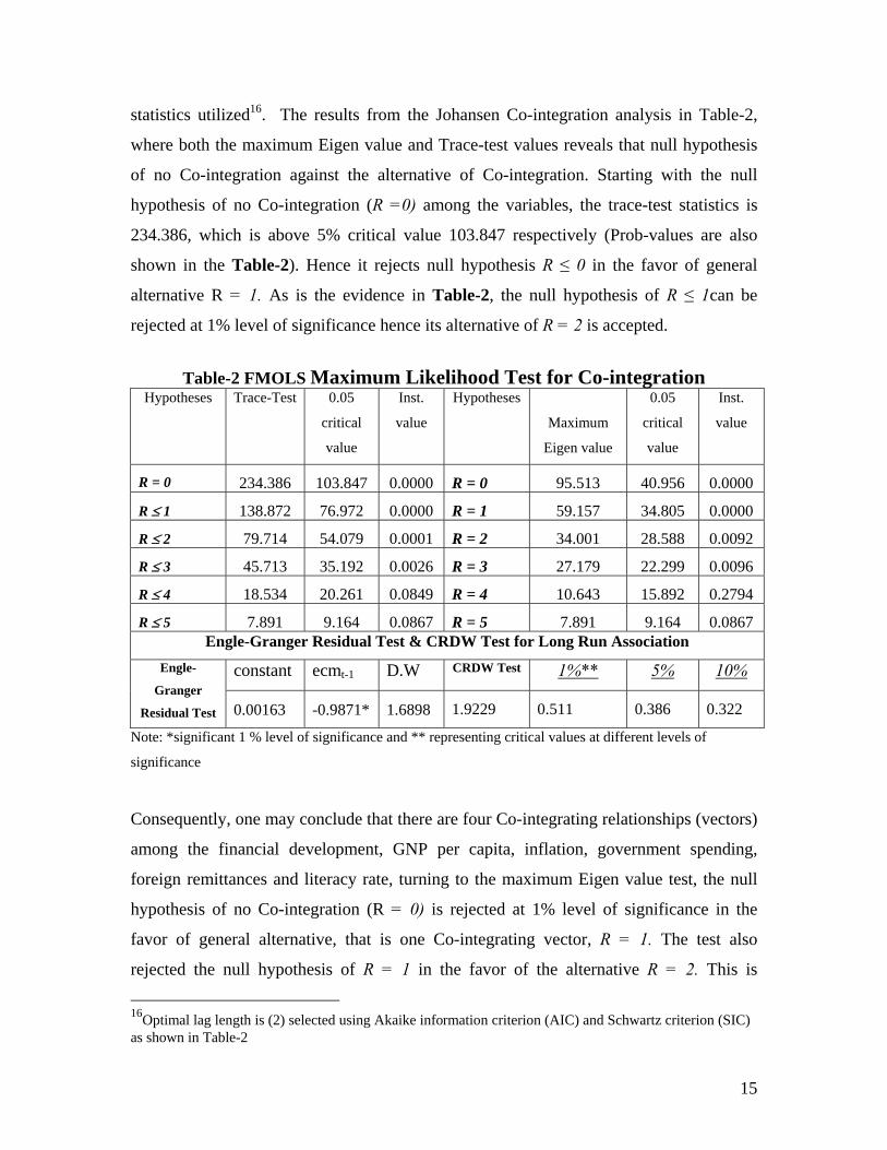
statistics utilized16. The results from the Johansen Co-integration analysis in Table-2,
where both the maximum Eigen value and Trace-test values reveals that null hypothesis
of no Co-integration against the alternative of Co-integration. Starting with the null
hypothesis of no Co-integration (R =0) among the variables, the trace-test statistics is
234.386, which is above 5% critical value 103.847 respectively (Prob-values are also
shown in the Table-2). Hence it rejects null hypothesis R ≤ 0 in the favor of general
alternative R = 1. As is the evidence in Table-2, the null hypothesis of R ≤ 1can be
rejected at 1% level of significance hence its alternative of R = 2 is accepted.
Table-2 FMOLS Maximum Likelihood Test for Co-integration
Hypotheses Trace-Test 0.05
critical
value
Inst.
value
Hypotheses
Maximum
Eigen value
0.05
critical
value
Inst.
value
R = 0 234.386 103.847 0.0000 R = 0 95.513 40.956 0.0000
R ≤ 1 138.872 76.972 0.0000 R = 1 59.157 34.805 0.0000
R ≤ 2 79.714 54.079 0.0001 R = 2 34.001 28.588 0.0092
R ≤ 3 45.713 35.192 0.0026 R = 3 27.179 22.299 0.0096
R ≤ 4 18.534 20.261 0.0849 R = 4 10.643 15.892 0.2794
R ≤ 5 7.891 9.164 0.0867 R = 5 7.891 9.164 0.0867 Engle-Granger Residual Test & CRDW Test for Long Run Association
constant ecmt-1 D.W CRDW Test 1%** 5% 10% Engle-
Granger
Residual Test 0.00163 -0.9871* 1.6898 1.9229 0.511 0.386 0.322
Note: *significant 1 % level of significance and ** representing critical values at different levels of
significance
Consequently, one may conclude that there are four Co-integrating relationships (vectors)
among the financial development, GNP per capita, inflation, government spending,
foreign remittances and literacy rate, turning to the maximum Eigen value test, the null
hypothesis of no Co-integration (R = 0) is rejected at 1% level of significance in the
favor of general alternative, that is one Co-integrating vector, R = 1. The test also
rejected the null hypothesis of R = 1 in the favor of the alternative R = 2. This is
16Optimal lag length is (2) selected using Akaike information criterion (AIC) and Schwartz criterion (SIC) as shown in Table-2
16
confirmed conclusion overall that there are four Co-integrating relationship amongst the
five I(1) variables. Therefore, over annual data from 1971 to 2005 appears to support the
proposition that in Pakistan, there exists a stable long-run relationship financial sector’s
performance and macroeconomic environment. Two tests also applied to investigate the
robustness of long run friendship among the variables in basic model. One can see results
of Engle-Granger & CRDW Residual Tests in lower part of Table-2. Results of these
said tets confirmed the robustness of long run association among the variables17.
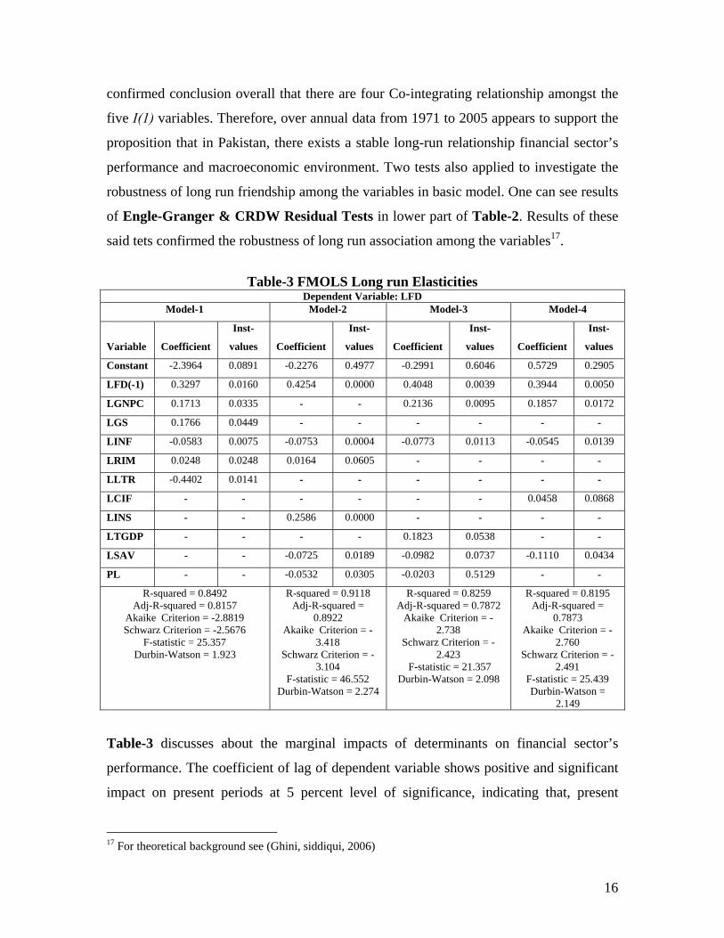
Table-3 FMOLS Long run Elasticities
Dependent Variable: LFD Model-1 Model-2 Model-3 Model-4
Variable Coefficient
Inst-
values Coefficient
Inst-
values Coefficient
Inst-
values Coefficient
Inst-
values
Constant -2.3964 0.0891 -0.2276 0.4977 -0.2991 0.6046 0.5729 0.2905
LFD(-1) 0.3297 0.0160 0.4254 0.0000 0.4048 0.0039 0.3944 0.0050
LGNPC 0.1713 0.0335 - - 0.2136 0.0095 0.1857 0.0172
LGS 0.1766 0.0449 - - - - - -
LINF -0.0583 0.0075 -0.0753 0.0004 -0.0773 0.0113 -0.0545 0.0139
LRIM 0.0248 0.0248 0.0164 0.0605 - - - -
LLTR -0.4402 0.0141 - - - - - -
LCIF - - - - - - 0.0458 0.0868
LINS - - 0.2586 0.0000 - - - -
LTGDP - - - - 0.1823 0.0538 - -
LSAV - - -0.0725 0.0189 -0.0982 0.0737 -0.1110 0.0434
PL - - -0.0532 0.0305 -0.0203 0.5129 - -
R-squared = 0.8492 Adj-R-squared = 0.8157
Akaike Criterion = -2.8819 Schwarz Criterion = -2.5676
F-statistic = 25.357 Durbin-Watson = 1.923
R-squared = 0.9118 Adj-R-squared =
0.8922 Akaike Criterion = -
3.418 Schwarz Criterion = -
3.104 F-statistic = 46.552
Durbin-Watson = 2.274
R-squared = 0.8259 Adj-R-squared = 0.7872
Akaike Criterion = -2.738
Schwarz Criterion = -2.423
F-statistic = 21.357 Durbin-Watson = 2.098
R-squared = 0.8195 Adj-R-squared =
0.7873 Akaike Criterion = -
2.760 Schwarz Criterion = -
2.491 F-statistic = 25.439 Durbin-Watson =
2.149
Table-3 discusses about the marginal impacts of determinants on financial sector’s
performance. The coefficient of lag of dependent variable shows positive and significant
impact on present periods at 5 percent level of significance, indicating that, present
17 For theoretical background see (Ghini, siddiqui, 2006)

17
performance of financial sector improves financial sector development in future more
that 34 percent. Increased real per capita as usual enhances the development of financial
sector at 5 % level of significance, there is 17 % improvement in the efficiency of
financial sector as real income rise by one percent. Coefficient of government spending
also tends to raise the effectiveness of financial sector development at “5 % level of
significance”. One may conclude that one percent increase in government spending
improves the financial sector’s efficiency by 17.7 percent.
Inflation has retarding effect on financial sector performance, more inflation means more
credit rationings and low money supply, obviously, fewer loans by financial
intermediaries to investment projects and there is decline in financial markets efficiency.
Furthermore, inflation will have contemporaneous effects on financial sector’s
performance. High inflation will increase the opportunity costs of holding money that
contracts the financial institution’s efficiency in inflationary environment. Further,
performance of financial sector lowers in high inflation atmosphere if nominal debts do
not increase rapidly as GDP (Butt, et, al, 2007). Continuous flows of international
remittances are having improving impacts on banking sector. Surprisingly, improvements
in human capital resource tends to push down the performance of financial
intermediaries, perhaps due to mismatch of education with financial sector requirements,
indicates that the skilled labor could not absorb the advanced technology to improve the
efficiency of financial sector.
Improvements in financial institution’s policies also stimulate banking sector to make
financial sector more progressive & efficient as in Model-2. As public savings perk up,
financial sector’s development declines in Pakistan. The main reason is that there is high
difference between lending and deposit rates (spread rate). In long run, people prefer to
invest their savings in real assets like, land, gold, government savings schemes, bonds
also in shares. The deposit rate on deposits is not attractive that’s why every body wants
to save his money in productive projects and definitely financial sector will have less
deposits in long span of time. Political instability also retards financial sector’s
development.

18
Model-3 & 4 expose that impact of trade and capital account openness which affects the
financial sector positively and significantly at 5 & 10 percent level of significance
respectively. Results are same as Law and Demetriades (2005), that simultaneous
openness to both trade and capital inflows has a positive influence on financial
development, in tandem with [institutions] hypothesis, the quality of country’s institutions
has a separate influence on financial development.
)11....(inflglg 10 0
650
40 0
3210
1 tt
n
j
n
j
n
j
n
j
n
jt
n
J
ecmlremlltrlsnpclfdlfd εηβββββββ ++Δ+Δ+Δ+Δ+Δ+Δ+=Δ −= === =
−=
° ∑ ∑∑∑ ∑∑o
Table-4 FMOLS Short Run Elasticities Dependent Variable: DLFD
Variable Coefficient T-Statistic Inst-valuesConstant -0.0154 -0.8489 0.4040 DLFD(-1) 0.2678 1.4744 0.1528 DLGNPC 0.2806 3.5070 0.0017 DLGS 0.1439 1.3434 0.1912 DLINF -0.0346 -1.5289 0.1388 DLLTR 0.3058 0.4397 0.6639 DLREM 0.0147 0.6437 0.5256 Ecmt-1 -0.8663 -3.0940 0.0048
R-squared = 0.653289 Adjusted R-squared = 0.556210
Akaike info criterion = -2.946946 Schwarz criterion = -2.584157
F-statistic = 6.729456 Prob(F-statistic) = 0.000156
Durbin-Watson stat = 1.595134
Table-4 gives results of ECM (Error Correction Model) formulation of above equation.
According to Engle-Granger (1987), Co-integrated variables must have in ECM
representation. In the case of small developing economy like Pakistan, this ECM strategy
provides solution for spurious correlation regarding short term dynamic relationship
financial development and its determinants. Whereas, the long run dynamics appears in
the set of regressors. Technically, ECM (Error Correction Term) works as a tool for
measuring the speed of adjustment back to Co-integrated relationships. According to
19
(Banerjee, et al, 1993) when integrated variables deviate, this ECM is a force which
affects them, so that, they return towards their long-run relation. Therefore, the longer is
the deviation; the greater would be the force tending to correct the deviation.
Short run dynamic behavior clearly indicates that picture is hopeful in short span of time.
The entire stream of performance indicators are having signs consistent with the theory
but insignificant except for GNP per capita which improves the performance of financial
sector. The short run dynamic impacts have maintained their signs even to the long span
of time. A fairly high speed of adjustment to the equilibrium level with correct sign after
a shock is illustrated by the equilibrium correction coefficient (Ecmt-1) estimated value of
-0.866, which is significant at 1 percent level of significance. The dis-equilibrium of
almost 86.6% from the previous year’s shock converges goes back to the long run
equilibrium in the current year.
Sensitivity Analysis
Finally, the cumulative sum (CUSUM) and the cumulative sum of squares (CUSUMsq)
are applied while analyzing the stability of the long-run coefficients together with the
short run dynamics. Pesaran and Shin (1999) suggested an empirical investigation of the
stability of estimated coefficient of the error correction model. A graphical representation
of CUSUM and CUSUMsq is provided in Figures 1 and 2. The null hypothesis (i.e. that
the regression equation is correctly specified) cannot be rejected, following Ouattara,
(2004) if the plot of these statistics remains within the critical bounds of the 5% level of
significance.
The plots of both the CUSUM and the CUSUMsq are with in the boundaries which are
quite evident from figures 1 and 2, therefore, the stability of the long run coefficients of
regressors (long run parameters) are confirmed by these statistics which affect country’s
financial sector’s development. In order to evaluate stability of selected model
specification the cumulative sum (CUSUM) and the cumulative sum of squares
(CUSUMsq) of the recursive residual test for the structural stability (see Mohsen, and
BahmaniOskooee, 2002) can be used. Since, neither the CUSUM nor the CUSUMsq test
20
statistics exceed the bounds of the 5 percent level of significance (see Figures 1 and 2), so
the model appears stable and correctly specified.
E. Conclusion Strong and sustainable macroeconomic situation are the requirements of any developing
country like Pakistan especially at the implementation of 3rd generation reforms for
financial sector in Pakistan. Certainly, the period from 2000 onwards witnessed rapid
growth of financial sector due to the reforms being introduced. Although the second half
of 1990s made the process of reforms comparatively costly as the entire economic
condition was not much favorable. To experience effectiveness and adequacy in reform
implementation and efficient functioning of the financial sector what is needed is sound
and favorable macroeconomic environment in the country. In order to compete in this fast
changing global economy, Pakistan still has to strive hard to achieve the required level of
development, in-spite of the fact that country’s financial markets have been liberalized
and operating on competitive basis. However, macroeconomic indicators require more
improvement because country still lags behind other developing countries in the region
with regard to financial deepening and intermediation. Several factors contributed
towards remarkable performance of Pakistan’s financial sector during 2000-05, like for
instance, comparatively favorable macroeconomic indicators, remittances flows,
outreach, product innovation, consumer financing, SME financing, etc
Empirical findings of the study reveal that previous policies of financial institutions and
economic growth improve the financial development. Rise in the level of government
spending and foreign remittances push the performance of financial sector in the upward
direction. Rising inflation deteriorates the efficiency of financial markets through its
damaging impact while literacy rate is having negative influence on banking sector in
Pakistan. Openness in trade and improvements in capital inflows open new directions to
enhance the development of financial markets in the country. Further more, performance
of financial sector is attached with qualified institutions. More qualified financial
institutions means more development in the financial sector. High savings rate declines
the efficiency of banking sector and political instability retards the performance of
21
financial markets. Thus, efforts are still underway for the creation of an enabling
environment for the development of financial sector while adopting forward-looking
strategies for overcoming the challenges of globalization. To conclude, the entire process
of liberalization created a mushroom growth of both of non-banking financial institutions
(NBFIs) and banks, giving rise to profit competitions and also their existence in Pakistan.
References
1. Aggarwal; Asli Demirguc-Kunt and Maria Soledad Martinez Peria, (2006), “Do Workers’ Remittances Promote Financial Development?”.
2. Aizenman, J. (2004). “Financial opening and development: evidence and policy controversies,” American Economic Review, 94(2), 65-70.
3. Aizenman, Joshua and Noy, I. (2004). “Endogenous Financial Openness: Efficiency and Political Economy Considerations,” Manuscripts, University of California, Santa Cruz.
4. Alessandria, G. and J. Qian (2005), “Endogenous financial intermediation and real effects of capital account liberalization,” Journal of International Economics, forthcoming.
5. Azariadis, C. and B. D. Smith (1996). ”Private Information, Money, and Growth: Indeterminacy, Fluctuations, and the Mundell-Tobin Effect.” Journal of Economic Growth 1: 309-332.
6. Banerjee, A. and Newman, A. (1993), “Occupational Choice and the Process of Development”, Journal of Political Economy, 101(2):274-98.
7. Beck, T. (2002), “Financial development and international trade. Is there a link?”, Journal of International Economics, 57: 107-131.
8. Beck, T., A. Demirguc-Kunt, and R. Levine (2003). Law, Endowments, and Finance. Journal of Financial Economics 70 (2): 137-181.
9. Becker and David Greenberg, (2004), “Financial development and International Trade, mimeo.
10. Bencivenga, V.R. and B. Smith (1991), “Financial intermediaries and endogenous growth”, Review of Economic Studies, 58(2), April: 195–209
11. Benhabib, J. and M.M. Spiegel (1994), “The role of human capital in economic development: Evidence from aggregate cross-country data”, Journal of Monetary Economics, 34: 143–173.
12. Bhargava, A. (1986), “On the Theory of Testing for Unit Roots in Observed Time Series,” The Review of Economic Studies, 53(3), 369-384.
13. Bittencourt, (2007), “Inflation and Finance: Evidence from Brazil”, CMPO Working Paper Series No. 07/163, Department of Economics, University of Bristol, 8 Woodland Road, Bristol BS8 1TN, UK..
14. Bittencourt, M. (2006). Financial Development and Inequality: Brazil 1985-99. Bristol Economics Discussion Papers 06/582.

22
15. Bowers, W. and Pierce, G., (1975), “The Illusion of Deterrence in Isaac Ehrlich’s Work on the Deterrent Effect of Capital Punishment”, Yale Law Journal, 85, 187-208.
16. Boyd, J., R. Levine, et al. (2001). ”The Impact of Inflation on Financial Sector Performance.” Journal of Monetary Economics 47: 221-248.
17. Boyd, John H., and Smith, Bruce D., (1996), “The Co-Evolution of the Real and Financial Sectors in the Growth Process”, World Bank Economic Review, 10, 371-96.
18. Boyd, John H., Ross Levine and Bruce D. Smith, (1996) “Inflation and Financial Market Performance,” Federal Reserve Bank of Cleveland, Working Paper 96-17.
19. Bum and Jeon, (2005), “Demographic Changes and Economic Growth in Korea” SKKU ERI WP-06/05.
20. Butt. M.S, Shahbaz. A and Nasir.N, (2007), “Inflation-finance Nexus: Case Study” memio.
21. Butler, D.; Merton, D. (1992), “The black robin: saving the world's most endangered bird”, Auckland, Oxford University Press.
22. Cameron, S., (1994), “A Review of the Econometric Evidence on the Effects of Capital Punishment”, Journal of Socio-economics, 23: 197-214.
23. Chinn, M. D. and Ito, H. (2005). “What matters for financial development? Capital controls, institutions, and interactions,” NBER working paper no. 11370.
24. Claessens, Stijn, Daniela Klingebiel and Sergio L. Schmukler (2002). “Explaining the Migration of Stocks from Exchanges in Emerging Economies to International Centers, “Policy Research Working Paper Series # 2816.
25. Coffee, J., (2000), “Convergence and its critics: What are the preconditions to the separation of ownership and control?” Unpublished working paper. Columbia University, New York.
26. Dejong, D.N., Nankervis, J.C., Savin, N.E., (1992), “Integration Versus Trend Stationarity in Time Series”, Econometrica, 60, 423-33.
27. Dickey, D., Fuller, W.A., (1979), “Distribution of the Estimates for Autoregressive Time Series with Unit Root”, Journal of the American Statistical Association, 74 (June), 427-31.
28. Ehrlich, I., (1975), “The Deterrent Effect of Capital Punishment – A Question of Life and Death”, American Economic Review, 65: 397-417.
29. Ehrlich, I., (1977), “The Deterrent Effect of Capital Punishment Reply”, American Economic Review, 67: 452-58.
30. Ehrlich, I., (1996), “Crime, Punishment and the Market for Offences”, Journal of Economic Perspectives, 10: 43-67.
31. Elliott, G., T.J. Rothenberg and J.H. Stock (1996), “E¢cient Tests for an Autoregressive Unit Root,” Econometrica, 64(4), 813-836.
32. Engle, R. F, Granger C. W. J. (1987), “Cointegration and Error Correction Representation: Estimation and Testing”, Econometrica, 55: 251–76.
33. Grossman, Gene and Elhanan Helpman, 2004, “Outsourcing in a Global Economy”, forthcoming, Review of Economic Studies.

23
34. Gupta, (1990), "Optimization in Groundwater Management", Keynote Address,, Proceedings, Second International Groundwater Conference, Kota Bharu, Malaysia, June 1990, pp.F1-F20.
35. Harris, R., Sollis, R., (2003), “Applied Time Series Modeling and Forecasting” Wiley, West Sussex.
36. Haslag, J. H. and J. Koo (1999). Financial Repression, Financial Development and Economic Growth. Federal Reserve Bank of DallasWorking Paper.
37. Huang, Y. and J. Temple (2005). Does External Trade Promote Financial Development? Bristol Economics Discussion Paper 05/575. University of Bristol, Bristol.
38. Huybens, E. and B. D. Smith (1998). ”Financial Market Frictions, Monetary Policy, and Capital Accumulation in a Small Open Economy.” Journal of Economic Theory 81: 353-400.
39. Huybens, E. and B. D. Smith (1999). ”Inflation, Financial Markets and Long-Run Real Activity.” Journal of Monetary Economics 43: 283-315.
40. Ito, Hiro (2004). “Is Financial Openness Bad Thing? An Analysis on the Correlation between Financial Liberalization and the Output Performance of Crises-Hit Economies” UCSC Working paper Series.
41. Johansen, S. (1992), “Co-integration in Partial Systems and the Efficiency of Single-Equation Analysis” , Journal of Econometrics, 52: 389–402.
42. Johansen, S., (1991), “Estimation and hypothesis testing of co-integrating vectors in Gaussian vector autoregressive models”, Econometrica, 59: 1551–80.
43. Johansen, Soren and Katarina Juselius (1990). “Maximum Likelihood Estimation and Inference on Cointegration- with Applications to the Demand for Money”, Oxford Bulletin of Economics and Statistics 52(2): 169-210.Pedroni, P. (2000). Fully modified OLS for heterogeneous co-integrated panels. In: Baltagi, B., ed. Non-stationary Panels, Panel Co-integration, and Dynamic Panels, Advances in Econometrics. Vol. 15, Amsterdam: JAI Press, pp. 93.130.
44. La Porta, R. et al. (1996), “Law and finance“, NBER Working Paper, No. 5661, July.
45. La Porta, R., F. Lopez-De-Silanes, A.Shleifer, and R.W. Vishny (1990). The Quality of Government. The Journal of Law, Economics, and Organization 15 (1):222-279.
46. La Porta, Rafael, Florencio Lopez-de-Silanes, and Andrei Shleifer, 2002, “Government Ownership of Banks,” Journal of Finance (Vol.57, No.1), pp. 265-301.
47. Law, S. H. and Demetriades, P. (2005). “Openness, institutions and financial development,” University of Leicester, working paper no. 05/08.
48. Layson, S., (1983), “Homicide and Deterrence: Another View of the Canadian Time Series Evidence”, Canadian Journal of Economics, 16: 52-73.
49. Levchenko, Andrei, 2003, “Institutional Quality and International Trade”, working paper, MIT.
50. Levine, R. (1997). Financial Development and Economic Growth: Views and Agenda. Journal of Economic Literature 35 (2):688-721.

24
51. Levine, R. and Renelt, D. (1992). “A sensitivity analysis of cross-country growth regressions,” American Economic Review, 82, 942-963.
52. Levine, Ross and Sergio L.Schmukler (2003). “Migration, Spillovers, and Trade Division: The Impact of Internationalization on Stock Market Liquidity,”University of Minnesota Working Paper.
53. Li, K., R. Morck, F. Yang and B. Yeung (2004). “Firm-specific variation and openness in emerging markets,” Review of Economics and Statistics, 86(3), 658-669.
54. Martell, Rodolfo and Rene Stulz (2003) “Equity Market Liberalization as Country IPOs,” NBER Working Paper # 9481.
55. Merton, R.C. (1992), “Financial innovation and economic performance”, Journal of Applied Corporate Finance, 4(4), winter: 12–22.
56. Mohsen, and BahmaniOskooee, Ng R.. W., (2002). Long Run Demand for Money in Hong Kong: An Application of the ARDL Model. International journal of business and economics, Vol. 1, No. 2, pp. 147155.
57. Ng, S., Perron, P., (2001), “Lag Length Selection and the Construction of Unit Root Test with Good Size and Power”, Econometrica, 69, 1519-54.
58. Orozco, Manuel and Rachel Fedewa, 2005. Leveraging Efforts on Remittances and Financial Intermediation. Report Commissioned by the Inter-American Development Bank.
59. Ouattara, B., 2004. Foreign Aid and Fiscal Policy in Senegal. Mimeo University of Manchester.
60. Pedroni, P. (1995). Panel co-integration: asymptotic and unite sample properties of pooled time series test with an application to the PPP hypothesis. Indiana University Working Papers in Economics, No. 95-013.
61. Pesaran, M. H., Pesaran, B. (1997). “Working with Microfit 4.0: Interactive Econometric Analysis”, Oxford: Oxford University Press.
62. Pesaran, M. H., Shin, Y. and Smith, R. J. (2001), “Bounds Testing Approaches to the Analysis of Level Relationships”, Journal of Applied Econometrics, 16: 289–326.
63. Phillips, P. C. B., Hansen, B. E. (1990). “Statistical inference in instrumental variable regression with I (1) Processes”. Rev. Econ. Studies 57:99.125.
64. Phillips, P.C.B. and P. Perron (1988), “Testing for a unit root in time series regression,” Biometrika, 75, 335-346.
65. Podpiera, R., 2004, “Does Compliance with Basel Core Principles Bring Any Measurable Benefits?” IMF Working Paper 04/204, (Washington: International Monetary Fund).
66. Rajan, R.G. and Zingales, L. (1998) Financial Dependence and Growth. American Economic Review, 88, 559-586.
67. Rajan, Raghuram G., Luigi Zingales (2003). “The Great Reversals: The Politics of Financial Development in the 20th Century,” Journal of Financial Economics 69.
68. Roediger, David R. (1999) “The wages of whiteness: race and the making of the American working class”, Rev. ed. London ; New York: Verso.
69. Schreft, S. L. and B. D. Smith (1997). ”Money, Banking, and Capital Formation.” Journal of Economic Theory 73: 157-182.

25
70. Shahbaz, M, Qureshi, M.N & Aamier, M, (2007), “Remittances and Financial Sector’s Performance: Under Two Alternative Approaches for Pakistan” Published in International Research Journal for Finance and Economics, 12, 2007, pp: 133-146.
71. Stulz, R. M. and Williamson, R, 2003, “Culture, openness, and finance,” Journal of Financial Economics, 70, 313-349.
72. Stulz, Rene (1999). “Globalization, Corporate Finance and the Cost of Capital,” Journal of Applied Corporate Finance, v12(3), 8-25.
73. Sundararajan, V., C. Enoch, A San Jose, P, Hilbers, R. Krueger, M. Moretti, and G. Slack, 2002, “Financial Soundness Indicators: Analytical Aspects and Country Practices.” IMF Occasional Paper No. 212, (Washington: International Monetary Fund).
74. Svaleryd and Vlachos, 2000, “Does Financial Development Lead to Trade Liberalization” mimeo.
75. Svaleryd, H., and J. Vlachos (2002), Markets for Risk and Openness to Trade: How are they Related? Journal of International Economics 57(2):369-395.
76. Venieris, Y.P. and D.K. Gupta (1986), “Income distribution and sociopolitical instability as determinants of savings”, Journal of Political Economy, 94(4): 873–884
77. Venieris and D.K. Gupta, (1986), “Income distribution and sociopolitical instability as determinants of savings”, Journal of Political Economy, 94(4): 873–884.
78. Wong, J., K.Choi, and T. Fong, 2005, “Determinants of the Capital Level of Banks in Hong Kong.” Hong Kong Monetary Authority Quarterly Bulletin.

26
Appendix-A Figure 1
Plot of Cumulative Sum of Recursive Residuals
-15
-10
-5
0
5
10
15
82 84 86 88 90 92 94 96 98 00 02 04
CUSUM 5% Significance
The straight lines represent critical bounds at 5% significance level.
Figure 2
Plot of Cumulative Sum of Squares of Recursive Residuals
-0.4
0.0
0.4
0.8
1.2
1.6
82 84 86 88 90 92 94 96 98 00 02 04
CUSUM of Squares 5% Significance
The straight lines represent critical bounds at 5% significance level.

![Final Report Shamim[1]](https://cdn.vdocuments.us/doc/165x107/547780975806b50b198b45b6/final-report-shamim1.jpg)


