C00-3072-121
Princeton University Elementary Particles Laboratory
Department of Physics
CHARM PRODUCTION BY MUONS AND ITS ROLE IN SCALE-NONINVARIANCE
George D. Gollin
October, 1980
Contract DE-AC02-76ER03072

•
. i
··-·· ... ,.:.·

CHARM PRODUCTION BY MUONS AND ITS ROLE
IN SCALE-NONINVARIANCE
GEORGE D. GOLLIN
A DISSERTATION
PRESENTED TO THE
FACULTY OF PRINCETON UNIVERSITY
IN CANDIDACY FOR THE DEGREE
OF DOCTOR OF PHILOSOPHY
RECOMMENDED FOR ACCEPTANCE BY THE
DEPARTMENT OF
PHYSICS
JANUARY, 1981
.fERMllAB~
,: LIBRARY.~. ...... . ... __ .;" - • .......i: ~..: ...
f~.·~~.~il-:~:-.;;..t ... ..wi-. .... t•·-· - ....... ---~-......... .:.._ .... ......r.1\

..

For Melanie
"0 frabjous day! Callooh, Callay!"
-Lewis Carroll


ABSTRACT
Interactions of 209 GeV muons in the Multimuon
Spectrometer at Fermilab have yielded more than 8xl0~ events
with two muons in the final state. After reconstruction and
cuts, the data contain 20 072 events with (81+10)%
attributed to the diffractive production of charmed states
decaying to muons. The cross section for diffractive charm
muoproduction is 6.9±f :: nb where the error ·includes
systematic uncertainties. Extrapolated to Q2=0 with
o(Q 2)=a(O)(l+Q2/A 2)-2 , the effective cross section for 178
(100) GeV photons is 750±f~g (560±~g~) nb and the parameter
A is 3.3+0.2 (2.9+0.2) GeV/c. The v dependence of the cross
section is similar to that of the photon-gluon-fusion model.
A first determination of the structure function F2Cc~) for
diffractive charm production indicates that charm accounts
for approximately 1/3 of the scale-noninvariance observed in
inclusive muon-nucleon scattering at low Bjerken x.
Okubo-Zweig-Iizuka selection rules and unitarity allow the
muon data to set a 90%-confidence lower limit on the wN total cross section of 0.9 mb.


TABLE OF CONTENTS
ABSTRACT ............................................. LIST OF TABLES ...................................... LIST OF FIGURES .................................... .
Chapter I. INTRODUCTION .............................. .
I I.
I I I.
A brief history of the quark model Charm Models for charm production by muons The muon experiment
THE BEAM AND THE MULTIMUON SPECTROMETER
The muon beam The Multimuon Spectrometer
The magnet Hadron calorimetry Trigger hodoscopes and the dimuon trigger Wire chambers Data acquisition
RECONSTRUCTION AND ANALYSIS
Reconstruction Track finding Track fitting
Acceptance modeling Background modeling
71 ,' K decay Muon tridents, T pairs, bottom mesons
Extracting charm from the data General features of the data Systematic errors
Page
vii
xi
xiii
1
9
22
IV. RESULTS AND DISCUSSION .................... .
Acceptance correction Diffractive charm muoproduction cross section Virtual and real photoproduction of charm
Q2 dependence of the effective photon cross section
Contribution of charm to the rise in the photon-nucleon total cro~s section
v dependence of the effective photon cross section
The charm structure function The role of charm in scale-noninvariance The ratio of w production to charm production
and the ~N total cross section Conclusions
ACKNOWLEDGEMENTS .............................. · · · · · ·
Appendix A. DRIFT CHAMBER SYSTEM FOR A HIGH RATE
EXPERIMENT ............................... · ·
B. THE TURBO-ENCABULATOR ..................... .
REFERENCES .......................... · · · · · · · · · · · · · · · ·
TABLES ....................... · .. · · · · · · · · · · · · · · · · · · · ·
FIGURES ........................ · ·. · · · · · · · · · · · · · · · · · ·
x
67
87
89
94
97
102
llO

xi
LIST OF TABLES
Table Page
1. Calorimeter and hodo~cope subtrigger combinations resulting in a full dimuon trigger ....................................... 102
2. Mean values of six reconstructe.d kinematic quantities for data before background subtraction, for charm Monte Carlo, and for n, K-decay Monte Carlo ........................ 103
3. Effects of charmed quark fragmentation on daughter energy and acceptance ................ 104
4. The Q2 dependence of the virtual photoproduction cross section for charm ....... 105
5. The v dependence of the virtual photoproduction cross section for charm in the range .32 < Q2 < 1.8 (GeV/c} 2 ............. 106
6. The Q2 dependence of the charm structure function F2(c~) for two values of average v ... 107
7. Calculated lO~d F2 I d ln(Q 2) at fixed Bjerken x vs. v, Q2, and x ................... 108
..
•

x j ii
LIST OF FIGURES
Figure Page
1. Drell-Yan production of muon pairs through quark-antiquark annihilation .................. 111
2. Models for charmed particle production ........ 113
3. The NI beam line at Fermilab 115
4. Multiwire proportional chambers and scintillation counters in the muon beam 117
5. The Multimuon Spectrometer .................... 119
6. One module in the muon spectrometer ........... 121
7. A trigger hodoscope ........................... 123
8. Calorimeter subtrigger patterns for dimuon events ........................................ 125
9. Trigger hodoscope subtrigger patterns for dimuon events ................................. 127
10. Calorimeter subtrigger probability vs. shower energy ........................................ 129
11. Multiwire proportional chamber center-finding electronics ................................... 131
12. A drift chamber cell and preamplifier ......... 133
13. Logical flow in the track-fitting program ..... 135
14. cc pair mass in the photon-gluon-fusion model 137
15. Momentum transfer-squared in the photon-gluon-fusion model ............................ 139
16. Hadronic shower energy in the photon-gluon-fusion model 141
17. Daughter muon energy in the photon-gluon-fusion model ............................ 143
Energy lost by the photon-gluon-fusion model
beam muon in the
19. Distribution of interaction vertices in slabs
xiv
145
in a module for shower Monte Carlo events 147
20. Distance from vertex to meson decay point for shower Monte Carlo events ..................... 149
21. Probability vs. shower energy for a shower to yield a decay muon with more than 9 GeV of energy ........................................ 151
22. Charged multiplicity in simulated showers for 11, K mesons with more than 5 GeV of energy .... 153
23. Number of meson generations between virtual photon-nucleon interaction and decay muon in simulated showers ............................. 155
24. Decay probability for 11's and K's in simulated showers ............................. 157
25. Energy lost by the beam muon in simulated inelastic collisions .......................... 159
26. Momentum transfer-squared in simulated muon-nucleon inelastic collisions .................. 161
27. Feynman x for primary shower mesons with more than 5 Gev of energy in simulated showers ..... 163
28. Pf distributions for primary shower mesons with more than 5 GeV of energy in simulated showers ....................................... 165
29. Feynman x distributions for all secondary mesons before imposing energy conservation in simulated showers ............................. 167
30. p~ distributions for all secondary mesons before imposing energy conservation in simulated showers ............................. 169
31. Energy of hadrons which decay in simulated showers ....................................... 171
32. Muon momentum along z from simulated showers
axis for decay muon
33. Energy of produced muons for simulated shower
173
events satisfying the dimuon trigger .......... 175

34. Momentum perpendicular to the virtual photon f?r produced muorrs at the decay point in simulated shower events satisfying the dimuon
xv
trigger ....................................... 177
35. Neutrino energy for simulated shower events satisfying the dimuon trigger ................. 179
36. Feynman diagrams for muon trident production calculated by Barger, Keung, and Phillips 55
••• 181
37. Distributions in daughter muon energy for background-subtracted data, charm Monte Carlo, and 11, K-decay Monte Carlo ............. 183
38. Reconstructed vertex distribution for background-subtracted data and charm Monte Carlo ......................................... 185
39. Distributions in daughter muon momentum perpendicular to the virtual photon for background-subtracted data, charm Monte Carlo, and 11, K-decay Monte Carlo ............. 187
40. Distributions in energy transfer for background-subtracted data, charm Monte Carlo, and 11, K-decay Monte Carlo ............. 189
41. Distributions in momentum transfer-squared for background-subtracted data, charm Monte Carlo, and 11, K-decay Monte Carlo ............. 191
42. Distributions in missing (neutrino) energy for background-subtracted data, charm Monte Carlo, and 11, K-decay Monte Carlo ............. 193
43. Distributions in inelasticity for backgroundsubtracted data, charm Monte Carlo, and 11, K-decay Monte Carlo ........................... 195
44. Flux of transversely polarized virtual photons accompanying a 209 GeV muon ........... 197
45. Virtual photon polarization £ •••.••••••••••••• 199
46. O\/oT in the photon- gluon-fusion model ....... 201
47. ~in the photon- gluon-fusion model .......... 203
48. Diffractive charm photoproduction cross sections ........................•............. 205
xvi
49. The role of charm in the rise of the rN total cross section ..... · ............................ 207
SO. Energy-dependence of the effective cross section for diffractive charm photoproduction . 209
51. Q2 dependence of the structure function F (cc) for diffractive charm muoproduction .... 211
2
52. Scale-noninvariance of F (c:C) 2
213

1
CHAPTER I
INTRODUCTION
A brief history of the quark model
There is great appeal in ascribing the rich
phenomenology of high energy physics to the interactions of
a small number of fundamental particles. Faced with a
growing zoo of subatomic particles, Fermi and Yang suggested
in 1949 that pions might be composite objects. 1 They boldly
calculated the properties that a nucleon-antinucleon state
would exhibit (antiprotons were not discovered until 1955)
and found them similar to those of the pion. In 1956 Sakata
proposed an extension to the Fermi-Yang theory to allow it
to describe strange particles. 2 Sakata's model used the
neutron, proton, and lambda as building blocks and predicted
the existence of several unusual (and nonexistent) particles
such as mesons with strangeness +2 and baryons with
strangeness -3 and isospin 1. 3 Six years later, Gell-Mann
and Ne'eman developed the "eight-fold way," a classification
scheme for mesons and baryons based on the group SU(3).~ The
"eight-fold way" of 1962 treated particle symmetries
2
abstractly, temporarily aba~doning the Sakata model's notion
of three fundamental hadron constituents. Encouraged by the
success of the SU(3) model, in 1964 Gell-Mann was "tempted
to look for some fundamental explanation of the situation." 5
He found that the observed hadron SU(3) multiplets could be
COnStrUCted from a Unitary triplet (d- S- u0) and a baryon
singlet b 0 • More interesting to Gell-Mann was a simpler
scheme which postulated three fractionally charged, spin 1/2
"quarks," each with baryon number 1/3. Baryons would be
composed of three quarks or four quarks and an antiquark,
etc. while mesons would be constructed from equal numbers
of quarks and antiquarks. 5 Soon after, Greenberg introduced
an extra degree of freedom, later to become color, into the
quark model to permit the symmetric combination of three
quarks in ans state. 6
Hadron spectroscopy provided ample experimental support
for the SU(3) symmetry of the "eight-fold way." Indications
that quarks themselves have physical as well as mathematical
significance came from several sources. The cross section
for inelastic electron-proton scattering may be written in
terms of two structure functions, W1
and W2
as
e:' E
Here, E and E' are the energies of the incident and
scattered electron, v is E-E', and Q2 is the square of the

3 .
four-momentum transferred from the electron. Experimenters
at the Stanford Linear Accelerator Center (SLAC) found that
W depended weakly on Q2 and that vW depended only on the 2 2
ratio Q2 /v. This suggested that beam electrons were
scattering elastically from point-like particles inside
target protons.
More support for the existence of quarks came from
measurements of muon-pair production in pion-nucleon and
proton-nucleon collisions. In the spirit of the quark
model, most non-resonant muon pairs should come from
quark-antiquark annihilation7 as shown in Fig. 1. Since
pions contain valence antiquarks while protons do not, the
ratio cr(pN*µ+µ-X)/0(11N+µ+µ-X) should be much less than 1.
This was seen to be true. 8
Charm
The unitary triplet, baryon singlet model discarded by
Gell-Mann led Bjorken and Glashow in 1964 to study a
constituent model for hadrons in which four fundamental
"baryons" were linked by SU(4) symmetric forces. 9 Baryon
number, electric charge, hypercharge, and a new quantum
number, charm, were conserved quantities in their theory.
They predicted that charmed mesons would have masses of
4
approximately 760 MeV and noted that their model was
"vulnerable to rapid destruction by the experimentalists." 9
Six years later, Glashow, Iliopoulos, and Maiani (GIM)
proposed another SU(4) charm model, this time a four quark
extension of Gell-Mann's three quark theory. 1 D The GIM model
eliminated strangeness-changing neutral currents from the
Weinberg-Salam model of weak interactions, which previously + -
had predicted anomalously high rates for the decays K~*µ µ + + -
and K .;..11 vv.
The w was discovered in proton-beryllium collisions and
in electron-positron annihilation in 1974. 11 Its narrow
width indicated that the w did not decay strongly and
suggested that it was a bound state of a new quark and its
antiquark, the charmed quark of the GIM model. The lightest
charmed mesons, the DD (1863) and D+(l868) were observed at
the Stanford electron-positron collider, SPEAR, in 1976.
The DD was seen as a narrow peak in the invariant mass + _++- +
di stri but ions of K 11 and K 11 11 11 systems and the D as a - + + I 2 bump in masses of K 11 11 states. The system recoiling
against the D was found to be always at least as massive as
the D, evidence for the associated production of the new
mesons. Excited states of the w and heavier charmed
particles such as the D'* , F, x, and Ac. have also been
observed. 1 3-
1 5
..

5
Models for charm production Er muons
In the simple quark model, nucleons are said to consist
of three valence quarks and a surrounding veil of sea quarks
and antiquarks. A beam pa t" 1 f r ic e can trans er energy and
momentum to a virtual charmed quark (or antiquark), creating
a charmed particle. F1"gure Za ·11 t h" 1 us rates t is process for
charm muoproduction. A more modern view holds that the sea
quarks arise from polarization of the vacuum by the strong
interaction field around the nucleon.
Another approach is provided by the vector-meson
dominance model (VMD), shown in Fig. Zb. In VMD, charm
production is a two step process. A virtual photon (y")
from the beam muon's electromagnetic field couples directly
to a vector meson, the ~. which then scatters off the target
into a pair of charmed particles. 16 The model assumes that
the Yv-~ coupling is nearly independent of Q2 and that the
~-N scattering is largely diffractive so that the charmed
quarks in the exchanged~ appear in the final state. VMD
predicts the Q2 -dependence of the reaction yvN ~ ccX to be
(1 + Q2 /mi )- 2, the propagator for the virtual ~ in the
Feynman diagram of Fig. Zb. Here, c is a charmed quark and
c is its antiquark. The model does not predict the v
dependence of charm muoproduction. Unlike the simple quark
model, VMD predicts a strong correlation between the momenta
6
of the daughter particles. VMD describes well the
production of the light particles p, w, and~. The larger
extrapolation from Q2 = 0 to Q2 = ~ required for charm
production however is unsettling. 16
A recent model for heavy-quark muoproduction is the
virtual photon-gluon-fusion (yGF) model. 17 Figure Zc shows
the Feynman diagram for yGF charm production. A virtual
photon from the beam muon fuses with a gluon from the
target, producing a charmed quark and antiquark. A cc pair
with suff1"c1"ent i"nvar·a t f · 1 n mass can ragment into a pair of
charmed particles. YGF uses elements of quantum
chromodynamics (QCD) and makes the following assumptions
about the production process. The scale of the strong
coupling constant, ~, is set by the mass of the charm
system. Color bookkeeping, the exchange of gluons between
the cc pair and the target to "bleach" the quark pair of
color, is assumed to be a soft process which does not change
the yGF predictions. The production process is assumed to
be unaffected by the fragmentation of quarks into hadrons.
Ordinary part on model calculation rules are used, allowing
results to be expressed as cross sections for
Yv -parton ~ ctX, summed over the contents of the nucleon and
integrated over the momentum distributions of the partons. 16
The Y GF model requires some numerical input before it
can make predictions. The mass of the charmed quark must be
specified. The distribution of momentum fraction for
gluons must be
definition of as
properties of
must be fixed.
completely the
dependence, the
defined.
must be
the nucleon
Once these
kinematics
cc pair
7
The mass constant A used in the
chosen. Parameters describing
target, such as -t dependence,
are set, the model describes
of charm production. Q2 and v
mass spectrum, and the total
production cross section are defined. 16 When a prescription
is adopted to allow the quarks to fragment into hadrons, the
yGF model describes charmed states observable in the
laboratory. The predictions of yGF will be discussed in
detail later.
The' muon experiment
This thesis describes interactions of the form µ~µµX
observed in the Multimuon Spectrometer (MMS) at Fermilab.
Brief descriptions of the results obtained from these
observations have appeared in Refs. 18 and 19. Data from
approximately 4xl0 11 21S GeV beam muons were collected
during the first half of 1978. Results from l.388xl0 11
positive and 2.892xl0 10 negative beam muons are presented,
covering the range 0 (GeV/c) 2 J. Q2 J. SO (GeV/c) 2 and
SO GeV J. v J. 200 GeV. After reconstruction and cuts, the
datp contain 20 072 events with two muons in the final
8
state, most from the production and decay of charmed
particles. The statistical power of such a large sample,
~so times that of other muon experiments', allows a first
measurement of differential spectra for charm muoproduction.
Chapter II describes the beam system and muon
spectrometer. Chapter Ill describes event reconstruction,
acceptance modeling, and background modeling. Extraction of
the charm signal, general features of the data, and
estimation of systematic errors are also discussed. Chapter
IV presents results of measurements of the diffractive charm
muoproduction total cross section, the Q2 and v dependence
of charm virtual photoproduction, and the role of charm in
ihe rise with energy of the photon-nucleon total cross
section. The contribution of charm production to the scale
non-invariance observed in muon-nucleon scattering at low
Bjerken x is discussed. A lower limit on the llJN total cross
section is presented.
..

9
CHAPTER II
THE BEAM AND THE MULTIMUON SPECTROMETER
Muons from the Nl beam line at Fermilab arrived at the
south end of the muon laboratory, passed through the air gap
of the Chicago Cyclotron Magnet (CCM), and entered the
Multimuon Spectrometer (MMS). The trajectories of beam
muons and any scattered or produced muons were registered by
wire chambers placed periodically in the MMS. Data from
events satisfying any of four sets of trigger requirements
were recorded on magnetic tape for subsequent analysis.
The muon spectrometer was conceived as a detector for a
high-luminosity muon scattering experiment studying rare
processes with one or more muons in the final state. Good
acceptance for both high-Q2 scattering events and low-Q2
multimuon events was desired. An intense muon beam incident
on a long target could provide the desired luminosity while
a spectrometer sensitive to muons produced at large and
small angles to the beam could meet the acceptance
requirements.
The detector was built in 1977 as a distributed target
dipole spectrometer.
into eighteen closely
Magnetized iron plates were grouped
spaced modules. Each module was
10
instrumented with wire chambers and hadron calorimetry. The
spectrometer was active over its entire fiducial area,
including the region traversed by the beam, allowing
reconstruction of low-cf multimuon events.
The beam system and individual elements of the
Multimuon Spectrometer will be described below. Further
details are presented in the appendices.
The muon beam
A schematic diagram of the Nl beam line is shown in
Fig. 3. A primary beam of 400 GeV protons from the main
ring was focused onto a 30 cm aluminum target. A series of
quadrupole magnets, the
the produced particles
quadrupole triplet train, focused
into a 400 m long decay pipe.
Particles of one sign and with momentum near 215 GeV/c were
bent west in enclosure 100 and were passed to enclosure 101.
An east bend at enclosure 101 acted as a momentum slit and
bent the beam away from its lower-energy halo. Polyethylene
absorber inside the west-bending dipoles of enclosure 102
stopped hadrons in the beam. Quadrupoles in enclosure 103
refocused the beam and an east bend at enclosure 104 made
the final momentum selection. Th~ Chicago Cyclotron Magnet
bent the beam east into the MMS. 20

11
Figure 4 shows the locations of multi-wire proportional
chambers (MWPC's)
to measure the beam
and plastic scintillation detectors used
and reject halo muons. MWPC's and
scintillator hodoscopes after the quadrupoles in enclosure
103 and at the entrance to enclosure 104 measured the
horizontal positions of muons. MWPC's and scintillator
hodoscopes measured horizontal and vertical coordinates at
the downstream end of enclosure 104, at the entrance to the
muon lab, immediately downstream of the CCM, and immediately
upstream of the MMS. Halo muons were detected at three
points upstream of the spectrometer. A "jaw" scintillation
counter in enclosure 104 registered muons which passed
through the iron of the enclosure's dipoles. A very large
wall of scintillation counters downstream of the CCM also
detected halo muons. A scintillator hodoscope with a hole
for the beam covered the front of the muon spectrometer and
counted halo particles entering the detector. A signal from
any of the halo counters along the beam disabled the MMS
triggers. Scintillation detectors in the beam counted
incident muons and vetoed events with more than one muon in
an rf bucket or with muons in the preceding or following
buckets.
Data were taken with 10 13 to l.7xl013 protons/spill on
the primary target. Typically l.9xl06 positive muons/spill
in a beam 8 inches high and 13.5 inches wide survived all
vetoes. An equal number were present in the halo outside
12
the beam. The fraction of positive muon flux which
satisfied all the veto
10 13 protons on target to
requirements varied from 1/2 with
3/8 with l.7xl0 13 protons on
target. The effective yield of positive beam muons was
about l.4xl0-7
muons/proton. The yield of negative muons
was one-third to one-half as great.
The beam energy was 215 GeV with a +2% spread. A
comparison between beam energies determined by elements in
the beam line and by the MMS showed that the values from the
beam line were systematically 1.5 GeV greater than those
from the muon spectrometer. A further check came from
elastic • production data with three final state muons.
Requiring that the beam energy equal the sum of the energies
of the final state muons showed the beam system's
measurement to be 2 GeV high. To maintain consistency
between beam energy and final state energy, the momentum
measured by the beam system was decreased during analysis by
about 1.5 GeV.
The Multimuon Spectrometer
The muon spectrometer consisted of four major systems.
Steel slabs served as an analyzing magnet and rectangular
scintillation counters measured hadronic shower energies.
•
•

13
Trigger hodoscopes determined event topologies and wire
chambers sampled muon trajectories. The detector is shown
in Fig. 5; each of its four systems will be described below.
The magnet
The most massive component of the detector was the 475
tons of steel that served as target and analyzing magnet.
The steel was rolled and flame cut into ninety-one plates,
each 4 inches thick and 8 feet square. They were grouped
into eighteen modules, with five slabs per module. An
additional slab was placed upstream of the first detector
module. The fiducial area was magnetized vertically to 19.7
kG by two coils running the length of the spectrometer
through slots in the steel. The magnetic field was uniform
to 3% over the central l.4xl m area of the slabs. It was
mapped with 0.2% accuracy using flux loops. The location of
the peak + -in theµ µ pair mass spectrum at 3.1 GeV/c from
events
µ N>-µ lji x, + -\j>rµ µ
provided confirmation that the field measurements were
correct. The polarity of the magnet was reversed
periodically. Roughly equal amounts of data were recorded
with each polarity.
14
The magnet steel also acted as a target. The upstream
single slab and slabs in the first twelve modules gave a
target density for the dimuon trigger of 4.9 kg/cm 2. This
corresponded to a luminosity of 500 events/pb for the data
presented here. Acceptance was fairly uniform over the full
target length. The average density of matter in the
spectrometer was 4.7 gm/cm 3, six-tenths that of iron,
allowing the magnet to act as a muon filter. Particles were
required to travel through the steel of six modules, almost
eighteen absorption lengths, before satisfying the µµ
trigger. Hadronic showers developed in the steel downstream
of interactions and were sampled every 10 cm by
plastic-scintillator calorimeter counters.
Hadron calorimetry
Figure 6 shows a side view of a single module.
Calorimeter scintillation counters 31.5 inches high by 48
inches wide were placed after each plate in the first
fifteen modules. Each counter was viewed from the side by
one photomultiplier tube. To achieve the large dynamic
range required, signals from the tubes were amplified in two
stages and the output from each stage was recorded by an
analogue-to-digital converter.

15
Deep inelastic scattering data and ~ production data
provided calorimeter calibration information. Magnetic
measurements of energy lost by muons in inelastic scattering
events related calorimeter pulse heights to hadronic shower
sizes. The calorimeter's zero level was set with the help
of ~ events which had less than 36 GeV of shower signal. By
requiring agreement between the average beam energy and the
average visible energy in the final state (the sum of the
three muons' energies and the calorimeter signal), a
zero-shower-energy pulse height was determined. The rms
accuracy of the hadron calorimetry was 6E=l.5E~ for 6E and
E in GeV, with a minimum uncertainty of 2.5 GeV.
Trigger hodoscopes and the dimuon trigger
Each of the spectrometer's eight trigger hodoscopes was
composed of four large "paddle" counters and eight narrow
"stave" counters. The arrangement of scintillator elements
in a trigger bank is shown in Fig. 7. Hodoscopes were
placed in the gaps following every other module, starting
with the fourth. The muon experiment took data using four
different triggers,
single-muon trigger
run in
required
parallel.
each of three
The hi gh-Q2
consecutive
trigger banks to have no hits in any stave counter and to
16
have a hit in a paddle counter. The three-muon trigger
required each of three consecutive banks to have hits
corresponding to three particles with some vertical opening,
perpendicular to the bend plane. The "straight-through"
trigger required a beam muon to enter the spectrometer
without passing through any of the upstream halo counters
and was prescaled by typically 3xl0 5• The two-muon trigger
required both a shower signal from the calorimetry and a
pattern of hits in three consecutive trigger hodoscopes
downstream.
The dimuon calorimeter subtriggers are illustrated in
Fig. 8. Calorimeter counters were ganged in overlapping
ciusters of ten. The first cluster included scintillators
in modules one and two, the second in modules two and three,
etc. giving a total of fourteen clusters. When signals
from at least half the counters in a cluster exceeded a
threshold level, that cluster's calorimeter subtrigger was
enabled. The greater range in steel of hadronic showers
enabled the
electromagnetic
calorimetry
cascades.
to discriminate against
The ho do scope subtriggers
required at least two counters to fire in the upstream pair
of a group of three consecutive banks comprising the
trigger. To reduce the rate of spurious triggers from
o -rays, the downstream bank was required to have hits in two
staves with at least one empty stave between them, or hits
in one paddle and any other counter, or hits in any three
..

17
counters. There were six different hodoscope subtriggers,
corresponding to each combination of three successive
trigger banks. Possible hit patterns satisfying a hodoscope
subtrigger are shown in Fig. 9. The full dimuon trigger
required both a calorimeter and a hodoscope subtrigger, with
a separation along the beam direction between them. The
upstream end of the earliest calorimeter cluster
participating in the trigger was required to be at least
seven modules from the furthest downstream trigger bank in
the trigger. Table 1 lists possible calorimeter-hodoscope
subtrigger combinations and Fig. 10 shows the probability of
satisfying the calorimeter subtrigger as a function of
shower energy. The subtrigger probability was measured when
the calorimeter was calibrated. It was found by determining
the fraction of the deep inelastic showers of given energy
which set calorimeter subtrigger bits. The hodoscope
subtrigger rate was typically l.3xHl 3 per beam muon while
the ful 1 di muon trigger rate was about 8xHl6 per beam muon.
Wire chambers
A system of nineteen
(MWPC's) and nineteen
multiwire proportional
drift chambers CDC's)
horizontal and vertical positions of muons
chambers
measured
in the
18
spectrometer. An MWPC and a DC were placed upstream of the
first module and in the gap following each of the eighteen
detector modules. The spatial resolution of the chamber
system was sufficient to allow multiple Coulomb scattering
of muons in the steel magnet to limit the spectrometer's
momentum resolution. The chambers were active in the beam
region, greatly reducing the sensitivity of the dimuon
detection efficiency to Q2 and pT. The wire chambers were
built on aluminum jig plate, permitting them to be thin but
rigid. This minimized the required widths of the
inter-module gaps and maximized the average spectrometer
density. The "low-Z" jig plates covered the upstream sides
of the chambers and served to stop soft electron 6-rays
traveling with beam muons.
The multiwire chambers had a single plane of sense
wires, measuring coordinates in the horizontal (bend) plane.
Signals induced on two high-voltage planes were read by
center-finding circuitry shown in Fig. 11, yielding vertical
and diagonal coordinates. There were 336 sense wires spaced
1/8 inch apart in each MWPC. High-voltage wires spaced 1/20
inch apart were ganged in groups of four, giving 196
diagonal channels and 178 vertical channels of information
with an effective channel spacing of 1/5 inch. The
proportional chambers were built on 1/2 inch jig plate and
were active over an area 41.5 inches wide by 71.2 inches
high. The separation between sense and high-voltage planes

19
was 0.4 inches. The MWPC readout electronics were gated on
for 70 nsec.
The chamber resolution was approximately equal to the
wire spacing divided by IT2. The efficiencies of the
multiwire chambers varied with position across the faces of
the chambers and with chamber location along the
spectrometer. Chambers near the front of the MMS had sense
and induced plane efficiencies in the beam of 83% and 59%
respectively while MWPC's towards the
induced plane efficiencies in the
rear
beam
had sense and
of 88% and 76%
respectively. Away from the beam, all proportional chambers
had sense and induced plane efficiencies of 95% and 94\
respectively.
Each drift chamber was built with a single sense plane
of fifty-six wires measuring coordinates in the bend plane.
Track finding with proportional chamber information resolved
the left-right ambiguity present in single plane DC's. The
drift cells were 3/4 inch wide with field shaping provided
by high-voltage planes spaced 1/8 inch from the sense plane.
The separation between high-voltage wires was 1/12 inch.
Figure 12 illustrates the drift cell geometry and indicates
the voltages applied to the field-shaping wires. The DC's
were active over a 42 inch wide by 72.5 inch high area and
were built on 5/8 inch aluminum jig plate.
The chamber preamplifiers read differential signals
from the transmission lines formed by sense wires and the
20
eight closest field-shaping wires as indicated in Fig. 12.
A start pulse sent from the trigger logic to the drift
chamber time digitizing system enabled a 120 MHz timing
clock. Signals from the chambers arriving at the digitizer
within thirty-one time bins of the start pulse were latched,
though most valid pulses arrived in an interval
approximately twenty bins wide. The drift chamber readout
was designed to latch up to four hits per channel with an
average of
described
Appendix A.
1/2 scaler per wire. The system has been
in detail in Ref. 21 which has been reproduced in
The resolution of the drift chambers was determined to
be better than 250 microns by fitting muon tracks with drift
chamber information. An experimental lower limit on the
resolution was not determined. The theoretical resolution
was 150 microns. The efficiency of the drift chambers was
better than 98% in the beam.
Data acquisition
Data from the different systems were read from the
experimental hardware by CAMAC whenever a trigger was
satisfied. A PDP-15 received the CAMAC information and
stored it on magnetic tape. On-line displays, updated after

21
each accelerator spill, permitted constant monitoring of the
performance of the detector while the experiment was
running. There were typically fifty triggers per spill; the
maximum number that could be processed was about twice that.
The data transfer rate of the CAMAC system and the data
handling speed of the computer set the limit on event rate.

22
CHAPTER III
RECONSTRUCTION AND ANALYSIS
The muon experiment recorded more than 10 7 triggers on
1064 reels of computer
TRACK, analyzed raw data,
from the wire chamber
tape. A track-finding program,
constructing muon trajectories
information. Taking into account
multiple Coulomb scattering and energy loss, a track-fitting
program, FINAL, momentum-fit muon tracks found by TRACK. A
Monte Carlo program modeled the muon spectrometer,
generating simulated raw data which were analyzed by TRACK
and FINAL. Different physics generators permitted the Monte
Carlo to describe the detector's acceptance for both charm
production and background processes.
This chapter discusses event reconstruction and data
analysis. The first section describes the track-finding and
momentum-fitting algorithms. The second describes
acceptance modeling and the third describes background
simulation. The fourth discusses methods used to isolate
the charm signal from the backgrounds and the fifth presents
general features of the reconstructed data and Monte Carlo
simulations. The sixth details methods used to estimate
systematic errors.
23
Reconstruction
The goals of the reconstruction algorithms are
conceptually simple. TRACK and FINAL attempt to determine
the hadronic shower energy and the four-momenta of initial
and final state muons at the interaction vertex. The
implementation of these goals belies their simplicity,
however. The finding program, TRACK, contains about 25,000
lines of FORTRAN and the fitting program, FINAL, even more.
TRACK and FINAL analyze events of all four trigger
topologies; the algorithms' reconstruction of dimuon
triggers will be described below.
Track finding
Raw data from an event are unpacked and translated into
wire chamber hits, calorimeter scintillator pulse heights,
and latch information. A filter routine inspects patterns
of hits in the trigger hodoscopes. The filter requires the
hodoscope information to be consistent with all tracks
intersecting at a common vertex. About 22% of the triggers,
some caused by o -rays and by stray muons entering the top or
bottom of the detector, are discarded. The filter does not
reject legitimate events with extra tracks.

24
Proportional chamber "blobs" are constructed of
contiguous wire hits in each plane of the MWPC's. Since the
deadtime of a drift chamber preamplifier corresponds
typically to a drift distance of 2.5 mm, drift chamber
"blobs" are constructed of all hits whose drift distances
are within 2.5 mm of the drift distance of another hit on
the same wire. MWPC hits in the planes measuring horizontal
(x), vertical (y), and diagonal (u) coordinates are grouped
into "triplets" or "matches" when any part of a u-plane blob
is within 0.75 cm of the location expected from the pairing
of a particular x blob and·y blob. A blob may participate
in at most three triplets; the matches are ordered by the
u positions. Both difference between predicted and found
triplets and blobs which are not part of a triplet are
available to the routines which search for tracks.
Calorimetric information gives an estimate of the
vertex position
algorithm finds
along
the
z, the beam direction. The vertex
maximum calorimeter counter pulse
height, A. For each slab in the detector it calculates a
quantity N, where N is the difference between the number of
counters with pulse height less than O.OBA and the number of
counters with pulse height greater than O.OBA, for all
counters upstream of that slab. The middle of the slab with
the largest value of N is chosen as the vertex position.
If several slabs share the largest value of N, the center of
the slab closest to the front of the detector is chosen.
25
TRACK uses data from the wire chambers in the beam
system to project a muon track into the detector. With
information from the MWPC between the first plate and the
first module, an incident position and angle for the beam
muon are determined. The trial trajectory is then extended
downstream using a fit which is linear in y and includes
energy loss and bending due to the magnetic field in x.
Chamber resolution and multiple scattering determine the
size of a search window at each MWPC. The triplet inside
the search window which is closest to the predicted location
is placed on the track. If no triplets are found, unmatched
blobs are used. TRACK recalculates the muon's trajectory
wi~h the new hits and projects downstream one
process is continued
calorimeter algorithm.
past the
After filling
vertex
in the
module.
found by
entire
The
the
beam
track with proportional chamber information, TRACK adds
drift chamber blobs to the muon's path. The two closest
blobs in each drift chamber are assigned to the track in one
pass, with no refitting after the inclusion of each DC's
data.
The track finder next searches for muon trajectories
downstream of the vertex. TRACK begins at the back of the
spectrometer and works upstream, constructing a trial track
with hits from at least four MWPC's. When a track is found,
drift chamber information is added simultaneously along the
entire trajectory. MWPC triplets used in the track are

26
removed from the list of available matches, then the program
begins the process again with the proportional chamber
information still available.
To project a track forward from the back of the MMS,
TRACK requires three triplets or two triplets and unmatched
x and Y hits in a third MWPC. The starting triplets may be
separated by up to three proportional chambers, but there
can be no more than one empty MWPC between any two chambers
in the initial segment of three MWPC's. Chambers used on a
track must have twelve blobs or less in the x plane. Within
resolution and multiple scattering limits, the y coordinates
must lie on a straight line. The curvature of the starting
segment must correspond to a momentum greater than 15
GeV/c -2o where a is the error of the calculated momentum.
Three-chamber track segments are extrapolated past the
vertex by a routine called TRACE. The actions taken by
TRACE are similar to those of the beam fitting routine. The
track is extended upstream one module at a time. A multiple
Coulomb scattering and resolution window is opened at each
chamber and a triplet or unmatched blobs are placed on the
track. TRACE refits the track with the new information,
including energy loss and bending in the magnetic field, and
continues upstream. When a track is complete, TRACE
simultaneously assigns the two best drift chamber blobs in
each DC to the track and removes all used triplets from the
table of available matches.
27
The track-hunting process continues until all possible
starting segments have been investigated. Tracks are
required to contain (x,y) points from at least four
proportional chambers with at least two of the points from
MWPC triplets. Tracks are also required to have a fit
momentum of less than 325 GeV/c. The x2 per degree of
freedom for tracks fit only with proportional chamber
information must be less than 4 or 5 for x or y views
respectively. Dimuon triggers with a reconstructed beam
track and two or more reconstructed final-state tracks are
written to secondary data tapes for analysis by
track-fitting program, FINAL.
Track fitting
the
FINAL assumes that tracks suffer smooth, continuous
energy loss. It fits tracks by simultaneously varying the
Coulomb scattering impulse in each module to minimize the x2
associated with the momentum fit. The algorithm calculates
iteratively, rejecting information which makes a substantial
contribution to the total x2 , then performing a new fit.
FINAL fits trajectories which are found by TRACK and then
attempts to constrain them to a common vertex.
Figure 13 diagrams the logical flow of the fitting
28
routine. The initial fit to all tracks uses only MWPC
information. The better drift chamber blob in each pair of
blobs is then attached to the track. FINAL attempts to
minimize the x2 of the fit and maximize the number of
chambers on the track by removing hits from the track and
replacing them with unattached DC blobs. Separate tracks,
corresponding to a single track broken by the track finder,
are fused. Halo tracks and tracks from stray muons are
identified and discarded. A vertex is then chosen for
dimuon triggers which possess a reconstructed beam track and
at least two accepted final state tracks.
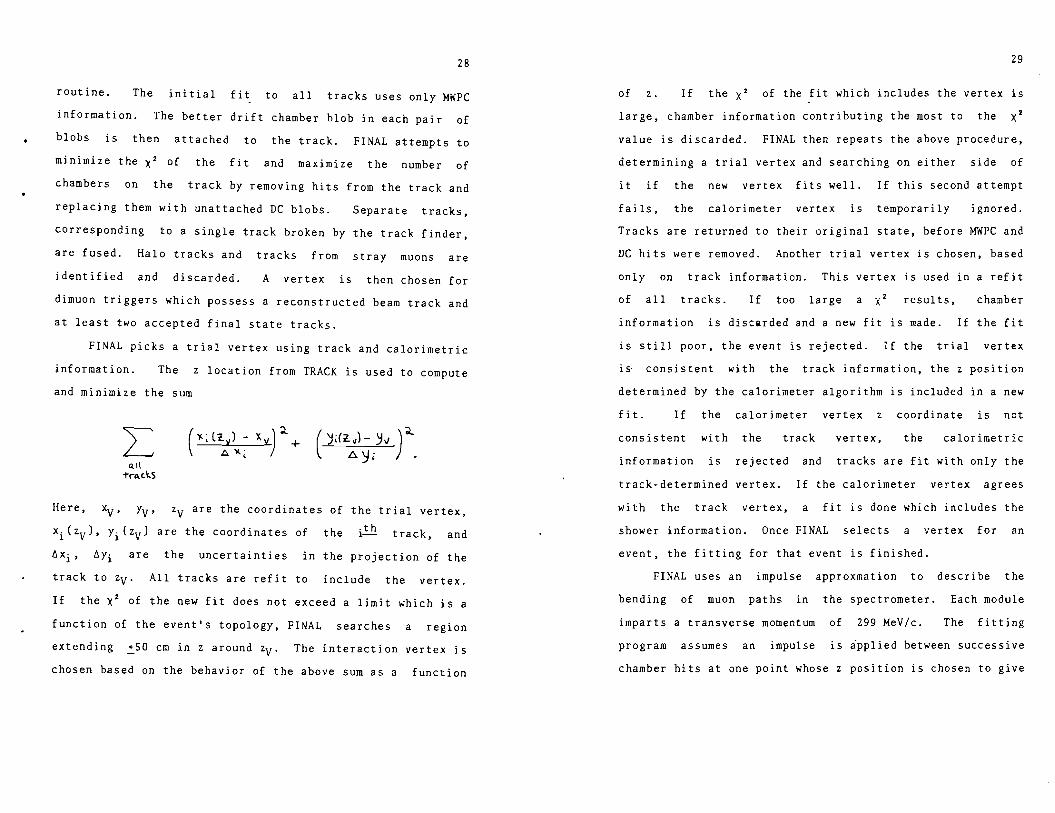
FINAL picks a trial vertex using track and calorimetric
information. The z location from TRACK is used to compute
and minimize the sum
Here, xv, Yy. zv are the coordinates of the trial vertex,
xi Czv), Yi Czv) are the coordinates of the ith track, and
~xi, ~Yi are the uncertainties in the projection of the
track to zy. All tracks are refit to include the vertex.
If the X2 of the new fit does not exceed a limit which is a
function of the event's topology, FINAL searches a region
extending ~SO cm in z around zy. The interaction vertex is
chosen based on the behavior of the above sum as a function
29
of z. If the x2 of the fit which includes the vertex is
large, chamber information contributing the most to the x2
value is discarded. FINAL then repeats the above procedure,
determining a trial vertex and searching on either side of
it if the new vertex fits well. If this second attempt
fails, the calorimeter vertex is temporarily ignored.
Tracks are returned to their original state, before MWPC and
DC hits were removed. Another trial vertex is chosen, based
only on track information. This vertex is used in a refit
of all tracks. If too large a x2 results, chamber
information is discarded and a new fit is made. If the fit
is still poor, the event is rejected. If the trial vertex
is consistent with the track information, the z position
determined by the calorimeter algorithm is included in a new
fit. If the calorimeter vertex z coordinate is not
consistent with the track vertex, the calorimetric
information is rejected and tracks are fit with only the
track-determined vertex. If the calorimeter vertex agrees
with the track vertex, a fit is done which includes the
shower information. Once FINAL selects a vertex for an
event, the fitting for that event is finished.
FINAL uses an impulse approxmation to describe the
bending of muon paths in the spectrometer. Each module
imparts a transverse momentum of 299 MeV/c. The fitting
program assumes an impulse is ipplied between successive
chamber hits at one point whose z position is chosen to give
30
the correct angular and _spatial displacement for a muon
traveling through the iron magnet. Since FINAL fits tracks
assuming a smooth, continuous energy loss, the z position of
the impulse is generally not midway between the front of the
first plate and back of the fifth plate in a module.
FINAL's estimate for the amount of energy lost by a particle
is a function of energy and path length in matter.
Multiple Coulomb scattering of particles is also
described in the impulse approximation. FINAL
simultaneously varies the transverse impulse in x and y in
each module to determine a best fit to a trajectory.
The track fitting program corrects the beam energy as
described in the previous chapter. The correction is
applied to blocks of data, each containing about 5% of the
full data sample. All events in a block have the same sign
of beam muon and magnet polarity. The hadron calorimeter is
calibrated separately for each data block as described
previously. FINAL uses the appropriate set of calibration
constants for each event.
A series of cuts, to be described later, are applied to
reconstructed events to discard data taken in kinematic
regions where the spectrometer's acceptance changes rapidly.
Before these cuts are made, 91% of the successfully analyzed
events have tracks which reconstruct to satisfy the dimuon
trigger. After the cuts, 98% of the events meet this
requirement. Because of this, no attempt is made to require
31
analyzed events to satisfy the µµ trigger after
reconstruction.
To compute kinematic variables such as Q2 and v, the
analysis programs must decide which final state muon is the
scattered muon and which is the produced muon. The choice
is obvious when the muons downstream of the interaction have
opposite charges-- the scattered, or "spectator" muon is the
particle with the same charge as the beam muon. If both
muons have the same sign as the beam, the more energetic µ
is chosen as the spectator. When applied to opposite sign
pairs, this algorithm is successful 91% of the time.
The error in vertex placement varies from 15 cm to
several meters. It depends in part on the opening angle of
the final state muon trajectories and the "cleanliness" of
the calorimeter information. The rms momentum resolution is
about 8% and varies approximately as the square root of the
length of tracks in the spectrometer.
TRACK is able to reconstruct 39% of the exclusive
dimuon triggers, where "exclusive" refers to events which
satisfy only one trigger. Most rejected events emerge from
the track finder with fewer than two final state tracks.
FINAL successfully analyzes 37% of its input from TRACK.
Most failed dimuon triggers do not survive FINAL's attempts
to construct a vertex. These events largely are caused by
noise such as shower activity in the detector and do not
reconstruct to have two muons in the final state.

32
Acceptance modeling
A Monte Carlo simulation of the spectrometer is used to
unfold detector acceptance from measured distributions. The
Monte Carlo also allows an extrapolation of measured
distributions into kinematic regions outside the acceptance
of the detector. By using the calculation to estimate the
ratio of observed to unseen events, total cross sections may
be determined. To be successful, the simulation must
accurately model the geometry and sensitivity of the
spectrometer and must include effects such as energy loss
and multiple scattering of muons. An acceptable model of
the underlying physics governing interactions is needed to
properly describe acceptance and to allow extrapolation
outside the measured kinematic region.
The Monte Carlo simulation of the Multimuon
S ·sts of two parts, a shell and a physics pectrometer cons1
generator. The shell describes the detector, propagates
particles through the spectrometer, and writes simulated
data tapes when an imaginary interaction satisfies an event
trigger. The physics generator contains the model for the
d d d daug hter particles and process being studie an pro uces
hadronic showers with distributions intended to mimic actual
interactions. Generators for charm production, deep
inelastic scattering, vector-meson production, and n, K
production are among the routines that have been
the Monte Carlo shell.
33
used with
The shell uses randomly sampled beam muons recorded as
straight-through triggers during the course of the
experiment. The program propagates beam muons from the
front of the spectrometer to interaction vertices, causing
the muons to suffer energy loss from effects such as µ-e
collisions, muon bremsstrahlung, and direct electron pair
production. Simulated muon trajectories are bent by the
magnetic field and are deflected by single and multiple
Coulomb scattering processes. A nuclear form factor is used
in the description of large-angle scatters. Daughter muons
bend, lose energy, and multiple scatter in the same way.
One of the physics generators creates charged n and K mesons
and allows them to decay after traveling through typically
half a module. The Monte Carlo causes the mesons to lose
energy, multiple Coulomb scatter, and bend in the magnetic
field during their brief existence. All muons are traced
through the spectrometer until they leave the detector or
stop. Interactions which satisfy any of the experimental
triggers are encoded and written to tape with the same
format as was used to record real events.
The shell assumes that the efficiency of the drift
chambers is iOO% and the efficiency of the MWPC's is less,
as described earlier. Wire chamber hits are generated to
represent particles traveling through the MMS and showers

34
developing downstream of an interaction. Halo muons,
a-rays, and out-of-time beam particles are not simulated.
Only a minimal attempt is made to model the spreading of
hadronic showers through the chambers.
A photon-gluon-fusion (YGF) model for charmed quark
production, described in chapter I, serves as the heart of
the physics generator used to study detector acceptance for
charm. In yGF, the cross section to produce a charmed quark
and its antiquark with a virtual photon is
for transversely polarized photons and
for longitudinally polarized photons. 22 Here,
and I
I
( d y. ol ~ ~ .;i. ) ( m" + ,,.1"' ~ J s"' 1~ ' Xo
- ~ ( """ ~(,.'- Q') ;,.•) }
w,, ~ ) J, ., GM, i; i ~r 91'- ~- -;(,.~.;it'. •·'l•·'•-.' )~~ ~D
-1> r-1:::~1 [1 - (3l'll.1- "mel.)~ + l.j {11-.\ Sm'rt1c" - ~m,-.) ~:i..
-a ... '( M< HM',.; -•·<' )b' l }
35
where
~"' (m .... +Q'l.)-1 ..,.o = ( ~ m ~ +a. 'l. ) I (.:i.1·11--1)
ols = 1~.,,. /t~H fa.l~m .... ) 1 Gt"'):. '?>(1-y.f/'1-.
The connection between muoproduction and virtual
photoproduction will be discussed in chapter IV.
Charmed quark pairs are produced quasi-elastically in
yGF; that is, the cc pair carries off most of the energy of
the virtual photon. To allow the model to make quantitative
predictions, the charmed quark mass, me, is set to 1.5
GeV/c 2•
22 The distribution for the gluon momentum fraction
xg is taken to be Here, is
(Q 2 + m ~ )/(ZMv). cc The strong coupling constant a s is
l.5/ln(4m ~ ) ~ 3/8. cc Figure 14 shows the
spectrum that results; the average pair mass is
mcc pair mass
4.9 GeV/c 2•
Only those events with mcc > ZmD are allowed to generate
final states containing open charm.
One-tenth of the beam muons which produce charm
interact coherently with iron nuclei while the rest interact
incoherently with nucleons in Fermi motion. The yGF model
does not describe the -t dependence of the production cross
section, where -t is the square of the four-momentum
transferred to the target. Coherence, screening, and -t
dependence are parametrized in a fashion identical to that
36
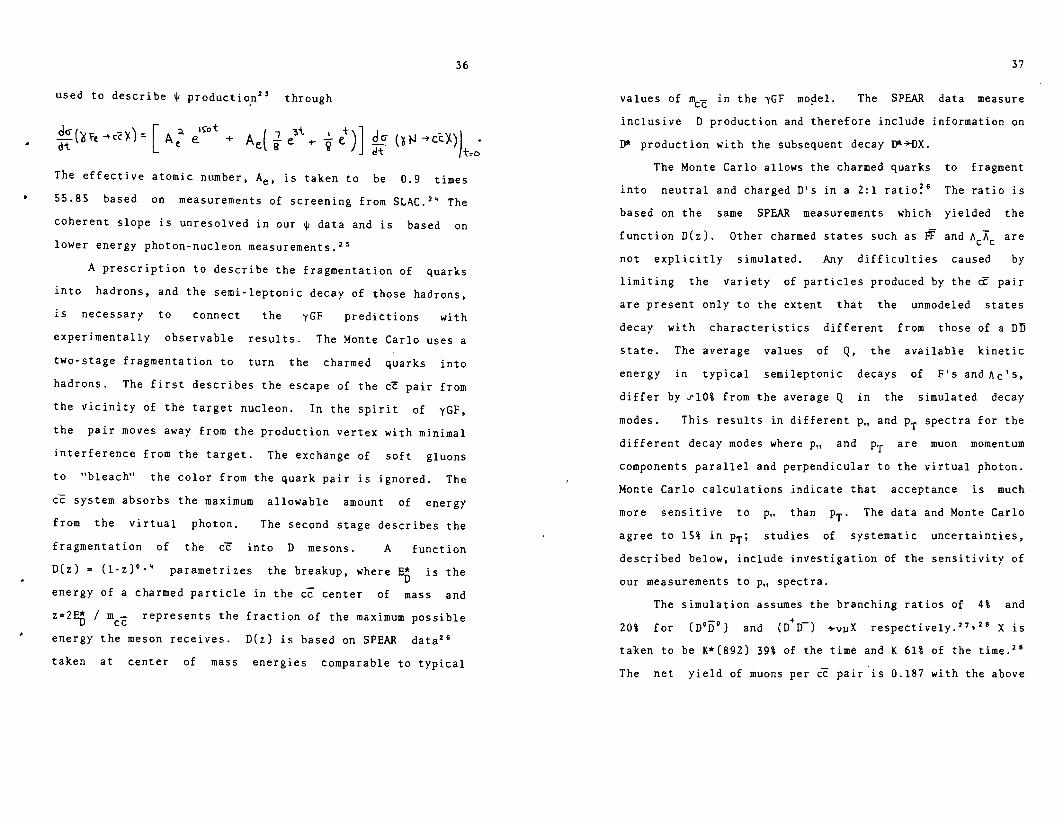
used to describe ~ producti~n 23 through
The effective atomic number, Ae, is taken to be 0.9 times
55.85 based on measurements of screening from SLAC. 2 ' The
coherent slope is unresolved in our ~ data and is based on
lower energy photon-nucleon measurements. 25
A prescription to describe the fragmentation of quarks
into hadrons, and the semi-leptonic decay of those hadrons,
is necessary to connect the -yGF predictions with
experimentally observable results. The Monte Carlo uses a
two-stage fragmentation to turn the charmed quarks into
hadrons. The first describes the escape of the cc pair from
the vicinity of the target nucleon. In the spirit of -yGF,
the pair moves away from the production vertex with minimal
interference from the target. The exchange of soft gluons
to "bleach" the color from the quark pair is ignored. The
cc system absorbs the maximum allowable amount of energy
from the virtual photon. The second stage describes the
fragmentation of the cc into D mesons. A function
D(z) = (l-z) 0·• parametrizes the breakup, where ED is the
energy of a charmed particle in the cc center of mass and
z=2E* / m - represents the fraction of the maximum possible D cc h · D(z) i's based on SPEAR data 2 6 energy t e meson receives.
taken at center of mass energies comparable to typical
37
· h GF d 1 The SPEAR data measure values of mcc in t e r mo. e .
inclusive D production and therefore include information on
D* production with the subsequent decay D*~DX.
The Monte Carlo allows the charmed quarks to fragment
into neutral and charged D's in a 2:1 ratio~ 6 The ratio is
based on the same SPEAR measurements which yielded the
function D(z). Other charmed states such as FF and AcXc are
not explicitly simulated. Any difficulties caused by
limiting the variety of particles produced by the Cf pair
1 h t t that the Unmodeled states are present on y to t e ex en
decay with characteristics different from those of a DD
state. The average values of Q, the available kinetic
energy in typical semileptonic decays of F's and Ac's,
differ by ~10% from the average Q in the simulated decay
modes. This results in different p11 and Pr spectra for the
different decay modes where p.. and PT are muon momentum
components parallel and perpendicular to the virtual photon.
Monte Carlo calculations indicate that acceptance is much
th P The data and Monte Carlo more sensitive to p.. an r· agree to 15% in Pr; studies of systematic uncertainties,
described below, include investigation of the sensitivity of
our measurements to p11 spectra.
The simulation assumes the branching ratios of 4% and
20% for (D 0o0) and (D+D_) ~vµX respectively. 27 • 28 Xis
taken to be K*(B92) 39% of the time and K 61% of the time. 28
The net yield of muons per cc pair is 0.187 with the above

38
assumptions. To permit prop~r modeling of the shower energy
and missing (neutrino) energy, D's are allowed to decay to
evX with the same branching fractions.
The Monte Carlo was used to generate a data set of
simulated events representing a beam flux equivalent to that
producing the real data reported here. In all, 2.87xl0~
incoherent and 3.30xl0f coherent Monte Carlo interactions
produced 4.49xl0¥ and 8.4xl03 triggers, respectively. The
trigger efficiency for YGF events with decay muons is
therefore 16.7\. Including the muonic branching ratios
indicated above gives a net trigger efficiency of 2.87%.
Figure 15 shows the Q~ distributions for events which
were generated by the charm model and which satisfied the
simulated trigger. The spectrometer's acceptance is
remarkably flat in Qa. due to its "no-hole" construction and
forward sensitivity. This is evident in the minimal
difference in the shapes of the generated and triggered
spectra. Figure 16 shows shower energy distributions. The
different shapes of the generated and triggered plots are
caused to great extent by the calorimeter subtrigger.
Spectra of daughter muon energies are shown in Fig. 17.
Since daughter muons must travel through at least six
modules to satisfy the dimuon trigger, the detector's
acceptance for slow muons is small. The energy loss per
module experienced by a muon is about 1 GeV and the
transverse momentum imparted by the magnetic field is about
39
300 MeV/c. Soft muons are s~opped or slowed and pitched out
of the spectrometer before they can trigger the apparatus.
Distributions in v are shown in Fig. 18. Acceptance as a
function of v, the energy lost by the beam muon, is
influenced strongly by the shower requirement and the
daughter-energy acceptance. For values of v close to the
beam energy, the requirement that the scattered muon travel
through more than six modules has a strong effect.
The data presented in figures 15-18 include both
same-sign and opposite-sign final state muon pairs. Since
beam muons are bent partially out of the spectrometer while
traveling to the interaction vertex, daughter muons with the
opposite sign are bent back into the MMS. Consequently,
after reconstruction, the acceptance for opposite-sign pairs
is higher by a factor of 1.45. After analysis cuts
described below, the factor decreases to 1.26.
The comparison between data and Monte Carlo samples
will be discussed later.
Background modeling
The experiment identifies charmed states by their
decays into a muon and at least two other particles. Since
decays such as D~Kn- contribute only to the calorimeter

40
signal, none of the kinema~ic distributions can exhibit an
invariant-mass peak representing charm production. To allow
extraction of the charm signal, important sources of
contamination must be modeled and subtracted from the data.
If the spectrometer had measured two-body decays which yield
mass peaks for charm, the experimental data would provide
all the necessary background information. A smooth curve
could be extrapolated under the mass peak, allowing accurate
determination of signal-to-background ratios. Since this is
not the case, a Monte Carlo simulation of the major
background is used to remove non-charm contamination from
the data.
The largest source of background is the decay-in-flight
of « and K mesons produced in inelastic muon-nucleon
collisions. Other sources of contamination are muon trident
production /"N ... ,..p .. µ- X, '(pair production~~p""C .. 'C- X with
-r .. ,µX, and bottom meson production p.N- }> BBX with B or
'B-,µ.x.
Tl, K decay
The average density of the Multimuon Spectrometer is
4.7 gm/cm3, six-tenths that of iron. Because of this, most
1f and K mesons produced in a hadronic shower interact and
41
stop in the detector before decaying. The probability for a
'tlor K with energy ¥me~ to decay in flight is L/(~c~) where
L is the particle's absorption length and~ is its mean
proper lifetime. For a 20 GeV 1f in the MMS the total decay
probability is about 4xl0-<1 , while for a 20 GeV KT- it is
4xl03 This indicates that perhaps a tenth of a percent of
the inelastic muon-nucleon collisions in the spectrometer
will give rise to a shower-decay muon. Since theoretical
estimates predict charm muoproduction cross sections that
are a percent or less of the total inelastic cross section,
accurate simulation of the 'fl, K decay background is
necessary.
A shower Monte Carlo based only on experimental data
measuring muon-nucleon and hadron-nucleon interactions is
used to study the lT, K-decay background. Parametrizations
f :i..o • :2'1,~o
o muon-nucleon scattering and hadron muoproduct1on
cross sections from the Chicago-Harvard-Illinois-Oxford
collaboration (CHIO) fix the Monte Carlo's absolute
normalization. Bubble chamber data are used to describe the
interactions ,,_,.,.
of pions and kaons with target nuclei as
the shower develops in the detector. The simulation creates
a full shower until all charged particles have energies less
than 5 GeV. Once the hadronic cascade has been generated,
the Monte Carlo chooses which, if any, of the shower mesons
to let decay.
The physics generator for the~. K Monte Carlo is used
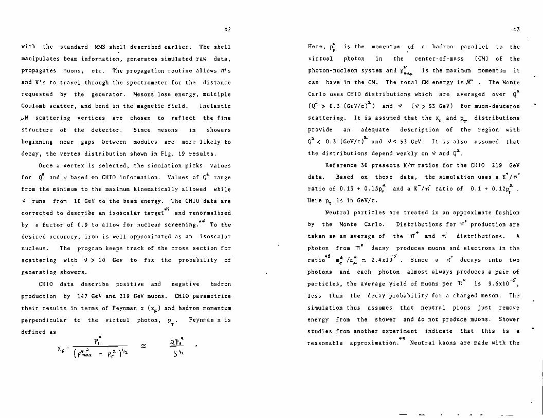
42
with the standard MMS shell described earlier. The shell
manipulates beam information, generates simulated raw data,
propagates muons, etc. The propagation routine allows rr's
and K's to travel through the spectrometer for the distance
requested by the generator. Mesons lose energy, multiple
Coulomb scatter, and bend in the magnetic field. Inelastic
~N scattering vertices are chosen to reflect the fine
structure of the detector. Since mesons in showers
beginning near gaps between modules are more likely to
decay, the vertex distribution shown in Fig. 19 results.
Once a vertex is selected, the simulation picks values
for Qa and v based on CHIO information. Values .of Q~ range
from the minimum to the maximum kinematically allowed while
~ runs from 10 GeV to the beam energy. The CHIO data are -11
corrected to describe an isoscalar target and renormalized
by a factor of 0.9 to allow for nuclear screening.~4 To the
desired accuracy, iron is well approximated as an isoscalar
nucleus. The program keeps track of the cross section for
scattering with v > 10 Gev to fix the probability of
generating showers.
CHIO data describe positive and negative hadron
production by 147 GeV and 219 GeV muons. CHIO parametrize
their results in terms of Feynman x (xF) and hadron momentum
perpendicular to the virtual
defined as
photon, p • T
Feynman x is
43
,.. Here, ~1 is the momentum of a hadron parallel to the
virtual photon in the center-of-mass (CM) of the
photon-nucleon system and pr _,,. is the maximum momentum it
can have in the CM. The total CM energy is .JS' The Monte
Carlo uses CHIO distributions which are averaged over Qa
(Qa > 0.3 (GeV/c).l.) and v (v > 53 GeV) for muon-deuteron
scattering. It is assumed that the xF and pT distributions
provide an adequate description of the region with
Q2 < 0.3 (GeV/c)a. and v < 53 GeV. It is also assumed that
the distributions depend weakly on v and Q2•
Reference 30 presents K/Tr ratios for the CHIO 219 GeV
data. Based on these data, the simulation uses a K,. /Tr+
a ratio of 0.13 + 0.13pT and a K-/TT- ratio of 0.1 + 0.12p"'
T
Here pT is in GeV/c.
Neutral particles are treated in an approximate fashion
by the Monte Carlo. Distributions for n" production are
taken as an average of the ,,-+ and n distributions. A
photon from 7T 0 decay produces muons and electrons in the . "8 .t a -~
ratio me Im,....-::::. 2.4xl0 Since a lf. decays into two
photons and each photon almost always produces a pair of 0 -!>
particles, the average yield of muons per 11 is 9.6xl0 ,
less than the decay probability for a charged meson. The
simulation thus assumes that neutral pions just remove
energy from the shower and do not produce muons. Shower
studies from another experiment indicate that this is a
"'" reasonable approximation. Neutral kaons are made with the
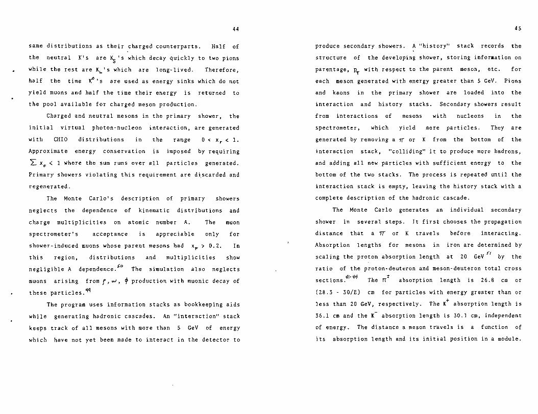
44
same distributions as their charged counterparts. Half of
the neutral K's are ~ 's which decay quickly to two pions
while the rest are K~'s which are long-lived. Therefore,
half the time t' 's are used as energy sinks which do not
yield muons and half the time their energy is returned to
the pool available for charged meson production.
Charged and neutral mesons in the primary shower, the
initial virtual photon-nucleon interaction, are generated
with CHIO distributions in the range O<XF<l.
Approximate energy conservation is imposed by requiring
L:, xF < 1 where the sum runs over all particles generated.
Primary showers violating this requirement are discarded and
regenerated.
The Monte Carlo's description of primary showers
neglects the dependence of kinematic distributions and
charge multiplicities on atomic number A. The muon
spectrometer's acceptance is appreciable only for
shower-induced muons whose parent mesons had xF > 0.2. In
this region, distributions and multiplicities show
negligible A dependence.so The simulation also neglects
muons arising from r' u.J' ~ production with muonic decay of
these particles.&!'!
The program uses information stacks as bookkeeping aids
while generating hadronic cascades. An "interaction" stack
keeps track of all mesons with more than 5 GeV of energy
which have not yet been made to interact in the detector to
45
produce secondary showers. A "history" stack records the
structure of the developing shower, storing information on
parentage, p with respect to the parent meson, etc. for T
each meson generated with energy greater than 5 GeV. Pions
and kaons in the primary shower are loaded into the
interaction and history stacks. Secondary showers result
from interactions of mesons with nucleons in the
spectrometer, which yield more particles. They are
generated by removing a 7f or K from the bottom of the
interaction stack, "colliding" it to produce more hadrons,
and adding all new particles with sufficient energy to the
bottom of the two stacks. The process is repeated until the
interaction stack is empty, leaving the history stack with a
complete description of the hadronic cascade.
The Monte Carlo generates an individual secondary
shower in several steps. It first chooses the propagation
distance that a 1T or K travels
Absorption lengths for mesons in
scaling the proton absorption length
before interacting.
iron are determined by
at 20 GeVn by the
ratio of the proton-deuteron and meson-deuteron total cross
sections.'ll-lf'f The TT:? absorption length is 26.8 cm or
(28.3 - 30/E) cm for particles with energy greater than or
less than 20 GeV, respectively. The K+ absorption length is
36.1 cm and the K absorption length is 30.1 cm, independent
of energy. The distance a meson travels is a function of
its absorption length and its initial position in a module.

46
Particles produced near the back of a module have a greater
chance of reaching the gap between modules.
The shower generator decreases the meson's energy by
the average amount it is expected to lose traveling through
the spectrometer to its interaction point.
inelastic collisions are simulated:
.. .. -; 0
T( N..., n,"TI- +n.._11 +~"11. +X
K~N..., n, K~ +n "11.'! +n -r.." +n rc0 +X :i. a •
The following
The coefficients n, -n4 are greater than or equal to zero.
These interactions are completely described by specifying
the particle multiplicity, xF, and distributions.
Charged multiplicities are taken from the bubble chamber
data of Refs. 33-36. Multiplicities are reduced by one unit
to remove the target proton from the bubble chamber
distributions. The data of Ref. 34 are then used to obtain
the xF "> 0 multiplicities from the corrected -1 <. xF < 1
multiplicities of the cited references. These forward
multiplicities provide an absolute normalization for the
momentum distributions used to generate secondary hadrons.
References 31, 32, 34, and 37 provide the Feynman x and p T
information which describes charged particle production.
Neutral pions are produced with distributions corresponding
to those for the pion with opposite charge from the parent
particle.
Secondary mesons with xF > 0 are generated. As before,
47
approximate energy conservation is imposed by requiring
2=_ xF < 1. After successful creation of a secondary shower,
all 1t 's and K's with more than S GeV of energy are loaded
into the two stacks.
The Monte Carlo neglects A dependence of secondary
multiplicities and momentum distributions. The data of
Ref. 45 indicate that the atomic number dependence is
important in the target fragmentation region, xF < 0, and is
negligible in the forward, positive xF region.
The simulation does not model associated production in
reactions such as irN-tKI\.
The entire cascade is generated before the Monte Carlo
chooses which particle will decay. If the probability of
decay for a typical shower meson were large, this method
would overpopulate the final generations of a shower. Early
decays in the shower would deplete the hadron population
available to produce ·more mesons in secondary cascades.
Since the probability for a 120 GeV shower to produce a
decay muon is about 1~3 , creating the full cascade while
initially neglecting decays is a sufficiently accurate
approximation. The Monte Carlo allows at most one meson to
decay. A hadron with at least S GeV of energy is chosen
based on a probability which is a function of absorption
length, energy, and place of creation in the MMS. The
probability that a particle will decay after traveling a
given distance is proportional to the probability that it

48
neither decayed nor interacted before getting that far.
Since it is much more likely for a TI or K to interact than
to decay, the simulation chooses the length of the hadron's
flight path according to the probability that it traveled
that distance before interacting. Figure 20 shows a plot of
the distance between creation and decay for chosen shower
mesons.
Pions decay to pv with 100% probability and kaons to;<"
with 63.5% probability. The 3.2% K..,µ.v1C decay mode is
neglected. The laboratory frame energy of the neutrino is
calculated to obtain the correct balance of shower energy,
daughter energy, and missing energy. Once a decay meson is
chosen, the shower generator returns program control to the
Monte Carlo shell. The shell propagates through the
detector all the mesons in the parent-daughter chain which
terminates in a decay, calculates the Lorentz
transformations needed to produce the resulting muon, and
propagates the muon through the rest of the detector.
Events which satisfy an event trigger are recorded on tape.
The total cross section for muon production via 1f,
K-decay is a convolution of the inelastic scattering cross
section with the probability that a decay muon comes from
the hadron cascade. The average beam energy at the
interaction vertex is 209 GeV. With that energy and the
beam's observed momentum spread, the inelastic cross section
to scatter with \l > 10 GeV is 3. 54_JJ- b. The cross section to
49
scatter and produce a decay_ muon with energy greater than 5
GeV is 2.28 nb. The combined trigger and reconstruction
efficiency for these events is 4.6%. Figure 21 shows the
probability vs. v for a shower to produce a muon with
energy greater than 9 GeV. The absolute normalization of
the Monte Carlo predicts that after reconstruction but
before analysis cuts, 43% of the dimuon signal is from rr, K
decay. After the analysis cuts described below, the decay
contamination drops to 19%.
The Monte Carlo was used to generate a data sample
corresponding to 1/3.915 times the beam flux represented by
the data to be discussed. All~. K-decay distributions and
th~ir errors are scaled by 3.915 to compare data with Monte
Carlo.
Figures 22-35 show predictions of the shower Monte
Carlo. The charged multiplicity for mesons with more than 5
GeV of energy is shown in Fig. 22. The number of meson
generations linking the virtual photon-nucleon interaction
and the decay muon is shown in Fig. 23. Though 22% of the
muons come from parent particles created in meson-nucleon
showers, after reconstruction and cuts this decreases to
10%. Figure 24 shows the decay
probability for generated shower mesons. The two peaks
correspond to ~·sand K's. The ratio of K's to ~·s decaying
in flight is 0.69 for KT/~~ and 0.46 for K- /-r{. The ratio
of rr~ to~ is 0.92. This unusual charge ratio accurately

so
reflects the production ratio of 0.91 measured by CHIO.
After reconstruction and analysis cuts, the ratios are 0.81 T 't - - + -for K In , 0.59 for K /~ , and 0.81 for TI /rr . The increase
in K/rr fractions presumably results from the difference in
acceptance caused by the greater available pT in K decay.
The change in the rt /Tr.- ratio is caused by the larger
acceptance for daughter muons charged opposite to the beam
since most data were taken with positive beam muons.
Figures 25 and 26 show v and Q~ for simulated inelastic
muon-scattering events. Figures 27 and 28 show the xF and :i.
pT distributions for rr•s and K's with more than S GeV of
energy in the primary shower. ' Distributions in xF and pT
for all secondary mesons before the l:xF requirement is
imposed are shown in figures 29 and 30. The approximate
energy conservation requirement rejects 14\ of the generated
secondary showers. Figure 31 shows the energy of hadrons
allowed to decay and Fig. 32 shows the decay muon momentum
along the z axis. The muon energy for events satisfying the
simulated dimuon trigger is shown in Fig. 33. Figure 34
illustrates the momentum component perpendicular to the
virtual photon for the muon at the decay point in events
satisfying a trigger. The neutrino energy for 1'(, K-decay
triggers is shown in Fig. 35.
It is important to have confirmation that the
predictions of the shower Monte Carlo are reasonable. Since
most reconstructed fr, K events have a muon from the decay of
51
a primary shower meson, data in agreement with the CHIO
results would provide this check. Unfortunately, all other
experiments studying hadron production by charged leptons
have used lower energy beams.sot The only possible tests of
the simulation are indirect.
One check compares the missing (neutrino) energy
predicted for Tr, K events with that observed in the data.
The meson momentum spectrum is sharply peaked at low
momentum.
Feynman x
This is caused by the approximate exp(-3.SxF) d.9 spectrum exhibited by primary mesons combined
4 '* (1-x.=) shape which describes secondary with the
production. Since the spectrometer's acceptance for slow
muons is small, decay muons produced in the forward
direction are strongly favored. A forward decay muon is
accompanied by a neutrino with very little energy in the
laboratory. The tGF charm model suggests that charmed
quarks tend to receive half of the virtual photon's energy.
Though fragmentation and decay kinematics exert a strong
influence on muon energies, the parent distribution of quark
momenta is not sharply peaked at low momentum. Charmed
particles tend to have more energy in the laboratory than
shower mesons so observed muons from charm can be produced
in a wider angular range. As a result, charm events should
show significantly greater missing energy. This is found to
be true; the comparison between dafa and Monte Carlo missing
energies will be discussed below.

52
Another effect influences the missing energy
distributions for T[, K and charm events. The probability
for a Tlor K to decay in flight is proportional to l/E where
Eis the meson's energy, while the probability for a charmed
particle to decay promptly is independent of energy. This
l/E dependence favors slow rr's and K's with a forward decay
muon over faster shower mesons with more decay phase space
in the acceptance of the MMS.
The results of the shower Monte carlo are consistent
with the rates predicted by a Monte Carlo used by the
Caltech-Ferrnilab-Rockefeller (CFR) neutrino experiment. sa
The CFR program uses a model by Feynman and Fields'+ to
generate a neutrino-induced primary shower. Data taken by
CFR with incident pions are used to parametrize secondary
interactions of shower mesons. The CFR Monte Carlo predicts
muon yields equal to those predicted by my shower simulation
for 75 GeV showers, 10% higher for 100 GeV showers, 15%
higher for 125 GeV showers, and 25% higher for 150 GeV
showers. The average shower energy in this experiment is 87
GeV.

53
Muon tridents, 'L pairs, bottom mesons
Other sources of background to the charm signal include
muon tridents, "( pairs with muonic decay of oner. and
bottom meson pairs with muonic decay of one or both mesons.
Each has been investigated and will be described.
Barger, Keung, and Phillips (BKP) have studied the
contribution of electromagnetic muon tridents to the . SS multimuon signal which might be seen by a muon experiment.
They wrote a computer program which generates trident events
through the three processes shown in Fig. 36. Since most
tridents are not accompanied by significant shower activity,
the BKP calculation predicts a small contribution to the
dimuon trigger rate. Events which satisfy the trigger and
are reconstructed as two-muon events should contaminate the
data at the level of 1/2%. The trimuon final state trigger
rate predicted by the BKP generator, when patched into a
crude simulation of the MMS, provides a consistency check of
the dimuon information. This check confirms that
electromagnetic tridents are a small background to charm
production.
Another upper limit on the trident background comes
from the study of events with three muons in the final state
which satisfied the dimuon trigger. This test checks the
consistency of the data with the hypothesis.that all the
54
dimuon triggers with three r~constructed final state tracks
result from charm production followed by the muonic decay of
both charmed particles. The production process and charm
d to be desc ribed by the dGF decay kinematics are assume
model discussed earlier. The charm Monte Carlo is
normalized so that it predicts the same number of dimuon
events after reconstruction and cuts as are present in the
data after subtraction of the expected 1t", K-decay
background. All data events and ~GF events which satisfy
the dimuon trigger with three reconstructed tracks are
subjected again to analysis cuts after the analysis is
blinded to the softest final state track. After cuts, 720
data events and 706 Monte Carlo events remain. Including
statistical errors, the Monte Carlo accounts for (98 ~ 5)%
of the data. This suggests that most 2µ events which result
from partial reconstruction of 3µ final states come from
·d t Less than one-fifth of charm systems, not muon tr1 en s.
the simulated dimuon triggers are caused by 3,JJ.charm events.
Consequently, other sources of 3p. events which feed down to
the 2,M- sample should account for a negligible fraction of
the data. We conclude that the dimuon background from
partially reconstructed muon tridents is small and neglect
it.
'L leptons can decay into hadrons and neutrinos. A '[
pair can therefore satisfy the di~uon full trigger through
decay combinations like -r·-. ,. ... \),; , 1:-- Ji\;...,._ Ye- The

SS
reduction in the trigger ra~e from muon tridents provided by
the calorimeter subtrigger therefore does not apply to
't'-pair events. Fortunately, the kinematics of lepton
production reduces the cross section for ~production by a
factor of (m-"'/m't):i. = 3.4xl0-3 relative to trident '18
production. Including the 17.S\ 'L->ry~ branching ratio
gives an extra factor of .289 so the net ratio of 't'
production with a single decay muon to trident production is
approximately 1~3 • The calorimeter subtrigger reduces the
dimuon trigger rate only by a factor of 160, so the ~
background should be about 0.1%, even less than the trident
background. The masses of the T and D are nearly equal.
Replacing the c~ by a r+~- and the gluon by a photon in
Fig. Z(c) allows a comparison of the charm and 'C cross
sections. The ratio is approximately
consistent with the above estimate.
background from 't' pairs is neglected.
Consequently, the
The ~GF model predicts a bottom meson production cross
section which is less than 0.03% of the charm cross . SS . section. Bottom pairs should be seen as dimuon events and
as events forming exotic charge combinations like
f-~N .. p. .. r_/A_ X from cascade decays through charm. The small
number of exotic events and events with four or five muons
in the final state proves that bottom production is not a
significant background to charm production. Our
90%-confidence upper limit on the cross section for "f
S6
production 56 confirms this conclusion. Even if the bottom
production cross section times muonic branching ratio were
100 times that for 'Y'•s, BB states would comprise less than
5% of the data.
Extracting charm from the data
Raw data and simulated raw data from the ~GF and "Tr,
K-decay Monte Carlo simulations are analyzed in an identical
fashion. Histograms for data and Monte Carlo are generated
with the same reconstruction and analysis cuts. After the
-rl, K histograms are scaled by 3.91S they are subtracted
bin-by-bin from the data histograms, yielding distributions
for charm. Statistical errors quoted for charm spectra
include the error on the subtraction. Systematic errors
associated with this procedure will be discussed below.
Cuts applied to
several purposes.
can be discarded.
data
Events
and Monte Carlo events serve
whose reconstruction is dubious
Data in kinematic regions where the
detector's acceptance changes rapidly or is poorly
understood can be rejected. Cuts which favor charm over 11,
K decay can improve the data's signal-to-background ratio.
A number of cuts are used to select events which are
well reconstructed. The vertex selection is checked by
57
requiring the difference between the z position of FINAL's
vertex and the calorimeter algorithm's vertex to be greater
than -60 cm and less than +65 cm. The incident energy of
the beam muon must lie between 206 GeV and 226 GeV. The ~~
for the fit to the beam track must be less than 10 for four
degrees of freedom in the horizontal view and less than 7.5
for three degrees of freedom in the vertical view. An
aperture cut passes events whose beam muons did not enter
the iron of the enclosure 104 dipoles. Events must have
exactly two reconstructed final-state tracks. Each track
must have horizontal and vertical ~2
fits with less than 4.5
and 3.5 per degree of freedom, respectively. The number of
degrees of freedom for tracks in the MMS depends on the
length of the tracks. Data which satisfy only the dimuon,
and not the trimuon, trigger are passed. Reconstructed
tracks are projected upstream to the vertex and downstream
until they leave the MMS. These "extended" tracks must be
missing no more than four MWPC hits between the hit furthest
downstream on the track and the point where the extended
track leaves the detector. There must be no more than six
missing chamber hits between the vertex and the hit furthest
upstream on the track. To reject events associated with a
shower entering the front of the spectrometer, the MWPC
upstream of the first module must contain fewer than ten
hits. Reconstructed tracks must differ sufficiently in
curvature and direction to represent distinct muon
58
trajectories. Two requirements discard events in which a
stale track has been interpreted as the trajectory of a
produced muon. The difference between the z momentum of the
beam and the sum of the z momenta of final state tracks must
be greater than -18 GeV/c. The ratio of the energy lost by
the beam muon to the energy observed in the final state (the
sum of the muon energies and the shower energy) must be
greater than 0.6.
Several analysis cuts exclude data from kinematic
regions where the spectrometer's acceptance changes rapidly
or changes in a way which is poorly modeled. Reconstructed
tracks are required to have at least 15 GeV/c of momentum.
Events are required to have more than 36.5 GeV of shower
energy.
of the
Reconstructed vertices must lie between the centers
first and eighth modules. To increase the
signal-to-background ratio, daughter muons are required to
have at least 0.45 GeV/c momentum perpendicular to the
scattered muon. In addition, the beam muon is required to
lose at least 75 GeV of energy.
The dimuon sample shrinks from 82 026 events after
reconstruction cuts to 20 072 events after both
reconstruction and analysis cuts are applied. The 1[,
K-decay background drops from 43\ of the data to 19\ of the
data. Qualitative features of the data and further
justification for some of the analysis cuts will be
discussed in the next section.

59
General features of the data
Figures 37-43 show distributions for the two Monte
Carlos and data after s bt t" f h ...r u rac ion o t e 1( , K-decay
background. Events in the histograms survived
reconstruction and cuts; acceptance has not been unfolded.
Events in Fig. 37 pass all the
analysis cuts except that no daughter energy requirement is
made and all events are required to have ~ ~ 150 GeV. The
unusual 'V cut increases the sensitivity of the predictions
of the Monte Carlo simulation to assumptions about charmed
quark fragmentation. The i"nvert d h' t e is ogram represents the
1f, K Monte Carlo, absolutely normalized to the beam flux and
scaled as described earlier. The upright histogram
represents data after subtraction of the 1<, K histogram.
The smooth curve shows the prediction of the ¥GF model,
normalized to the data after the standard analysis cuts are
applied. The horizontal bar indicates the rms resolution at
30 GeV. Figure 37 makes clear the need for a daughter
energy cut. Though both Monte Carlo samples, and presumably
the data, heavily populate the region of low daughter
energy, the detector's acceptance is too small to allow
reconstruction of many of these events. All other
histograms and results do not include events with daughter
energy less than 15 GeV.
60
The probability to obtain a calorimeter subtrigger as a
function of shower energy is shown in Fig. 10. Because of
the curve's steep rise at low energy, a minimum shower
energy requirement of 36.5 GeV is imposed.
Figure 38 shows the vertex distribution for subtracted
data and ~GF Monte Carlo. Agreement between them is best in
the front half of the spectrometer. The beam bends out of
the detector while traveling through it. Tracks of daughter
muons with the same charge as the beam therefore tend to
become shorter as the vertex moves downstream. Inaccuracies
in the algorithm used by the Monte Carlo to inject
shower-induced hits into the wire chambers have the greatest
effect on short tracks and therefore on events occuring in
the downstream half of the spectrometer. By cutting on
vertex position, the data whose acceptance is not well
modeled can be discarded.
The momentum of the daughter muon perpendicular to the
virtual photon is shown in Fig. 39. As in Fig. 37, data,
~GF, and 1(, K Monte Carlo events are shown. The horizontal
bar indicating rms resolution is 0.15 GeV/c wide. The cut
requiring 0.45 GeV/c daughter momentum perpendicular to the
scattered muon essentially demands that the daughterµ have
a P; which is nonzero by at least 3~. The number of
tridents contaminating the data is further reduced by this
cut. The mean pT for the subtracted data is 15\ higher than
for the charm Monte Carlo. This variable is sensitive to

61
assumptions about -t dependence, not part of the ~GF model,
so the disagreement does not necessarily reflect a problem
with the charm production model.
Figure 40 shows the energy lost by the beam muon for
data and both Monte Carlo data sets. All canonical cuts
except the v cut are imposed. The horizontal bar
illustrates rms resolution. The agreement between
subtracted data and Monte Carlo is spectacular. The Tf,
K-decay events have lower average \). The ratio of
subtracted data toll, K is small for large~ but is of order
unity for v < 75 GeV. To reduce sensitivity to the absolute
normalization of the shower Monte Carlo, data with
\J < 75 GeV are discarded. The dashed curve shows the
predictions of the charm Monte Carlo when the ~GF \)
dependence is replaced by a flat v dependence and the
fragmentation is changed to D(z) = b (z-1). ~
The Q distributions are shown in Fig. 41. Horizontal
bars indicate rms resolution. The 1l, K events tend to have
lower Q~ than the subtracted data. The ~GF model predicts a ~
Q. spectrum that is slightly higher than observed.
Figure 42 presents the missing energy for subtracted
data and the two Monte· Carlos. As expected, the mean
missing energy is substantially less in the 71, K sample than
in the charm sample. The mean missing energies are
4.45!0.53 GeV, 14.59+0.18 GeV, and 18.18+0.24 GeV for 1[, K
Monte Carlo, ~GF Monte Carlo, and subtracted data. The
62
horizontal bar indicates rms resolution and the arrow shows
the change in the centroid of the data which results if the
calorimeter calibration is varied +2.5%. The relationship
between shower energy and pulse height used in both Monte
Carlos is fixed by deep inelastic scattering events as
described in chapter II. This is an accurate description
for 1'f, K-decay events since they are inelastic scattering
events. The showers in charm events, in the °tGF picture,
are caused by the decay products of the charmed particles
since very little energy is transfered to the target
nucleon. Charm decays almost always include K's in the
final state. Since K's have shorter lifetimes and longer
absorption lengths than rr•s, there is no reason to expect
that the signature of a charm shower, which may be initiated
by two K's and a lf, will exactly match that of an inelastic
#-N collision, which usually does not contain fast strange
. 1 3o part1c es.
Figure 43 shows the inelasticity for data and Monte
Carlos. Inelasticity is defined as 1 - E(daughter /#') I v.
Mean values of reconstructed v, Q~, daughter energy,
inelasticity, missing energy, and momentum perpendicular to
the virtual photon are presented in Table 2. Particularly
in the case of Y, daughter energy, and missing energy, the
tabulation excludes the possibility that the dimuon data can
be explained by if, K-decay.

63
Systematic errors
After reconstruction, cuts, and background subtraction,
the data contain 16 376 events attributed to the production
and muonic decay of charmed particles. A sample this large
has considerable statistical power-- a total cross section
can be determined to a statistical precision of better than
1%. To understand the limitations on the accuracy of
results presented here, systematic errors must be
investigated. Systematic effects can come from two sources.
The backgrounds to charm production may be described
incorrectly or the acceptance of the muon spectrometer for
charm events may be simulated inaccurately.
The predictions of the shower Monte Carlo are sensitive
to the K/1f ratio in primary showers. This is .:l.'l,30
information which is least well determined by CHIO.
the
To
gauge the Monte Carlo's sensitivity to this ratio, showers
were generated with K/11 ratios of 0.4 for both signs. The
data of Ref. 30 are inconsistent with ratios this high.
Simulated trigger rates increased by 60% and the number of
shower events surviving the standard cuts increased by 73%.
Since only 10% of the ir, K events passing analysis cuts
come from the decay of secondary hadrons, the predictions of
the simulation are not sensitive to assumptions made about
the interactions of primary hadrons in the detector.
64
A synthesis of charm and shower Monte Carlo samples
provides a consistency check. The data are represented as a
combination of both simulations. By seeing how the relative
normalizations must be changed to fit different kinematic
distributions of the data, an estimate of the accuracy of
the Monte Carlos was obtained. It is not correct to fix the
1f, K normalization this way since it then becomes impossible
to test the ¥GF model against the data.
We conclude that the background description provided by
the shower Monte Carlo is accurate to within 50%.
Therefore, after analysis cuts, our best estimate is that
the decay in flight of TI and K mesons contributes (19~10)%
of the dimuon signal where the quoted error is systematic.
The acceptance of the muon spectrometer is by far most
sensitive to the energy spectrum of produced muons. The ~GF
model describes quasi-elastic charm production; that is, the
cc pair receives most of the energy of the virtual photon.
The charm model accurately predicts the v dependence of the
subtracted data. Varying the fragmentation function D(z)
used to create D's from cc pairs allows investigation of
this sensitivity. D(z) provides the link between v, which
is correctly modeled, and daughter energy. The form for o·+ 01.6
D(z) used in acceptance modeling is D(z) : (1-z) . 3 -f·S'
Remodeling with D(z) : (1-z) and D(z) c (l-min(z,0.99))
changes the detector acceptan-ce by -19% and +20%,
The exponent s in the "too soft" and "too respectively.
65
hard'' functions are more than 5~ from the value determined
at SPEAR.'6
The mean daughter energies which result are
presented in Table 3. Agreement in energy and other
distributions is spoiled by using the alternative
fragmentation descriptions.
When same-sign dimuon data and opposite-sign dimuon
data are analyzed separately, little change is seen in
data-to-Monte Carlo ratios. Cross sections based only on
same-sign or opposite-sign events differ by 3.5% from those
based on both signs.
Systematic uncertainties in rr, K modeling and charm
modeling are not expected to be significantly correlated.
An estimate of the total systematic error is made by
reanalyzing the data with different assumptions. Errors are
parametrized by (1) decreasing, (2) increasing by 50% the
subtracted shower background and by recalculating the
acceptance with the (3) softer, (4) harder fragmentation
function. The effects on results are obtained by
reanalyzing the data with each of the four systematic
changes, adjusting the ~GF normalization to yield the
observed number of events past cuts, and replotting or
recalculating acceptance-corrected information.
positive deviations from the canonical results are added in
quadrature to yield the positive systematic error and all
negative deviations are added in quadrature to yield the
negative systematic error. The results define bands of
66
systematic tolerance around observed distributions. Cross
sections presented in the next chapter will include
systematic errors of +28' and -20,.
67
CHAPTER IV
RESULTS AND DISCUSSION
The spectra in figures 37 and 39-43 reflect physical
processes seen through the prism of experimental acceptance.
By removing detector effects with a Monte Carlo simulation,
the nature of the underlying physics may be studied. This
chapter describes acceptance correction and presents
measurements of charm production by muons and virtual
photons. Results include the total diffractive cross
section for muoproduction of charm and the Q~ and v
dependence of virtual photoproduction of charm. The cross
section for charm production by real photons and its
contribution to the rise in the photon-nucleon total cross
section are discussed. The role played by charm in the
scale-noninvariance of muon-nucleon scattering at low
Bjorken x' is described. A lower limit on the
f~nucleon total cross section is presented.
68
Acceptance correction
Most spectra presented in the following sections are
differential in Qa or v. To unfold the experimental
acceptance, data, ff, K-decay Monte Carlo, and ~GF Monte
Carlo are placed in (ln(Q'l), ln(v)) bins. If Ao'(Q 2 ,\>) is
the number of events in the (ln(Q~), ln(V)) bin which
includes the values Q~ and v, the ratio of subtracted data
to charm Monte Carlo in a bin is
t:.rr(clo.-la) - t.cS(it,K)
t.6 ( lr~F)
For small bins, the ratio of the acceptances for subtracted
data and charm Monte Carlo will be constant across the width
of a bin. Because of resolution smearing, the measured ~
average values of Q and v in a bin will generally differ
from the true average values. The charm Monte Carlo is used ;I.. to calculate the shift between measured and true mean Q and
v. The acceptance-corrected
which results is
differential cross section
'Jl ti.~ (da:to.) - MS (Tr, I<'.)
AO'U~i::)
Here, ~(charm) is the cross section for charm production by ~
muons and Q and v are the corrected average values in the
bin. This procedure, which equates real cross sections with

69
Monte Carlo cross sections weighted by the ratio of
subtracted data to Monte Carlo, is used to obtain the
results presented in the following sections.
Diffractive charm muoproduction cross section
The measured
production by 209
cross section for +I·~
GeV muons is 6.9_,.4
diffractive charm
nb. "Diffractive
production" refers to the creation of cc pairs carrying most
laboratory energy of the virtual photon, as in the Of the
~GF and VMD models. This analysis is insensitive to
mechanisms which might produce charm nearly at rest in the
photon- nucleon center of mass. To correct for experimental
acceptance~ the cross section is computed by multiplying the
~GF prediction of 5.0 nb. by the ratio of subtracted data to
~GF Monte Carlo. A total of 20 072 data events, 944 Ti, K
Monte Carlo events (scaled to 3696 events), and 13 678 XGF
Monte Carlo events survived reconstruction and analysis cuts
to contribute to this ratio. The error on the cross section
is systematic and reflects uncertainties in background
subtraction and acceptance modeling, as described earlier.
The statistical uncertainty is negligible compared to the
systematic error. Ignoring nuclear shadowing and coherence
would raise the reported cross section by 9.4%. After a
70
(26:t5H relative acceptance correction, the opposite-sign to
same-sign ratio for background-subtracted data is 1.07~.06.
A Michigan State-Fermilab (MSF) experiment has reported
a cross section for charm production by 270 GeV muons of 3+1
nb.s1 °Correcting the beam energy to 209 GeV, using the ~GF
model, reduces the MSF cross section to 2.1+0.7 nb. The MSF
data contain 412 fully reconstructed dimuon events; the
collaboration simulates detector acceptance with a
phenomenological model containing three free parameters.SS
Their choice of parameters was based on a sample of 32
dimuon events observed earlier at a beam energy of 150
Gev.s' The 150 GeV sample contained an estimated 4.9 trident
events and a small, but unspecified, number of if, K-decay
events. Our results are inconsistent with the MSF
measurement.
Virtual and real photoproduction of charm
As a beam muon passes near a target nucleon, its
electromagnetic field may transfer momentum and energy to
the target. In the single-photon approximation, the
interaction is described as the absorption by the target of
a virtual photon from the beam particle. There is intuitive
appeal to characterizing the muon's field as a cloud of

71
virtual quanta-- classically, the field of a rapidly moving
charge behaves like a pulse
stationary .observer. 00 In the
of radiation as it passes a
spirit of this, the
differential charm production cross section may be written
The factors ~T and rl represent the fluxes of transversely
and longitudinally polarized virtual photons with mass'1.=-Q~
and energy v. The terms cr1 (Q~,Y) and ~~(Q~,v) are the cross
sections for photons of the two polarizations to be absorbed
by the target to yield charmed particles.
defining E =~Ir.,. and R= cr .. llfT gives
More compactly,
Parametrizations of ~ and f from Ref. 61 are used to
extract virtual photon cross sections from muon cross
sections:
rT = Cl (\>1+Q1.)''~
d...il Q'E1- 0-E-)
t_, = 1-t- 1( Ql.+\)l.) tc.n 1 ~
Q
Here, E is the beam energy, M is the nucleon mass, 9 is the
muon scattering angle in the laboratory, and (Bjerken) x is
7Z
Q'1.l(2Mv). Figure 44 shows Q:i.T'T vs. Q~ for different values
of \I; Fig. 45 illustrates the polarization ratio, E . The J. flux rT is normalized so that as Q approaches zero, the
effective cross section ~H =(l+fR)O'.,. approaches the cross
section for real photons of energy v.
Q~ dependence of the effective photon cross section
The effective photon cross section is obtained by
factoring the equivalent flux of transversely polarized
virtual photons out of the muon cross section. A
measurement of R would require a substantial amount of data
at a second beam energy and has not been made. There is no
reason to expect crL lcr.,. for charm production to equal a.Irr.,.
for deep inelastic scattering. In peripheral models like
~GF and VMD, the photon couples to the produced quark pair,
not to a valence quark in the target. Consequently, the
kinematic effects which determine R for charm are different
from those which influence R for inelastic scattering.
Figure 46 shows R as predicted by ~GF and Fig. 47 shows the
product ER. ~ The Q dependence of the effective photon cross section
is shown in Fig. 48 and Table 4 .. The data are grouped into
two 'V bins, covering the regions 75 GeV"- Y "- 133 GeV with
73
(i>) = 100 GeV and \) "> 133 GeV with (\l) = 178 GeV. In the
figure, data points are shown with statistical errors. The
solid lines are best fits to VMD propagators,
r5(0)(l+Q4 ;,{ )-d... The dashed curves, normalized to
the nominal value of ~(O), indicate the influence of the
systematic effects discussed previously. Systematic errors
are parametrized by (1) decreasing, (2) increasing by 50\
the subtracted ~. K-decay background and by recalculating
the acceptance with the (3) softer, (4) harder fragmentation
function described above. The mass parameter /\ is 3.3+0.2
GeV/c and 2.9+0.2 GeV/c for the 178 GeV and 100 GeV data,
respectively. E d Q~--o, h d xtrapolate to t e ata are best fit • 180 +•o•
by cf(O) of 750-no nb and 560_ 1l.0 nb for the 178 GeV and 100
GeV data. The errors on(\ and ~(0) are systematic. A drop ~ ;i.. ~ in ~et.f with decreasing Q is present below Q =.32 (GeV/c) .
Fits which do not include data in this region yield
essentially the same results.
A wide-band photon-beam experiment has measured cross
sections averaged from 50-200 GeV of 464~207 nb for n•i)i
pair productionbl. and, later, 295~130 nb for inclusive D0
lo3 ~· production. Using SPEAR data , one may crudely estimate
the neutral D:charged D:F: "-r: ratio to be 2:1:1:1 at
mcc - 4-5 GeV/ca.. The average of the two D0
cross sections
is 343~110 nb, corresponding to a total cross section for
charm production of -860 nb. This is consistent with our
measurement. The authors of Refs. 62 and 63 determine
74
experimental acceptance with a model which uses a
fragmentation function D(z)=f(z-1) and assumes no energy
dependence above 50 GeV. The dashed curve in Fig. 40 shows
that the muon data do not support these assumptions.
Contribution of charm to th~ r~se in the photon-nucleon total cross section
Above --40 GeV, the photon-nucleon total cross section
increases with "'1,loS energy. This rise presumably reflects "S" the "hadronlike properties" of the photon; most hadronic
total cross sections begin to rise in this energy region.
The authors of Ref. 65 suggest that charm production may
contribute 2 to 6ftb of this increase in the energy range
from 20 GeV to 185 GeV. A fit to half the photon-deuteron
cross section from Ref. 64 is shown in Fig. 49. Since the
threshold energy for charm production is about 11 GeV, the
charm cross section rises from zero at low energy to the
values reported here at v =100 GeV and v =178 GeV.
Diffractively produced charm is seen to make only a minor
contribution to the rise in the photon-nucleon total cross
section.

75
~ dependence of the effective photon cross section
The v dependence of the effective photon cross section
in ~ 2 01.
the range 0.32 (GeV/c) < Q < 1.8 (GeV/c) is shown in
Fig. so and Table s. For fixed v, the cross section cr'eff
varies by less than 20% in this range of Q~. Data in the
figure are shown with statistical errors. Systematic
uncertainties, parametrized as described previously, are
indicated by the shaded band, referenced to the solid curve
for visual clarity. To gauge the systematic error
associated with a given point, the shaded region should be
moved vertically until the position cut by the solid line
rests on the data point. Data with \) < 75 GeV are excluded
from the analysis because of their large systematic
uncertainty.
The solid curve exhibits the v dependence of the ¥GF
model with the gluon x' S'
distribution 3(1-ic,) Ix, and
represents the data
choices,
with 13% confidence. q
(1-Xs) /x'j and distribution s
(1-x_,) (13. S+l. 07 /xj) are indicated by dashed
Other gluon
"broad glue" 17
curves. The
dashed curve labeled "BN" represents the phenomenological bb
parametrization of Bletzacker and Nieh and the horizontal
dashed line represents energy-independence. All curves are
normalized to the data.
The muon data clearly indicate that O'(H increases with
76
photon energy. The standard "counting-rule" gluon
distribution is favored, but systematic uncertainties
prevent the analysis from ruling out the BN model or the two
extreme choices for the gluon x' distribution.
The charm structure function
In quantum mechanics, the probability for a free
particle in a state Ip) to scatter from a potential V(r)
into a state If'> is ]<r'l V(r)/p)I~ in familiar notation.
If the potential is localized in space and reasonably "well
behaved," the initial and final states are well approximated
by plane waves. Neglecting normalization, in
non-relativistic quantum mechanics, the scattering
probability becomes
Defining 1 to be p-p' and F(qa.) to be the Fourier transform
of the potential allows the scattering probability to be
written as IFCqa.)I~. By studying
the short-range nature of the
measured.
the scattering process,
potential V(r) can be
The high energy analogue of F(q~) in potential
scattering is the nucleon structure function F~(x,Q2
) in

77
deep inelastic lepton scattering. For muon-nucleon
collisions, the scattering cross section is
The variables x and y are Q:i../(ZMv) and v/E where M is the
nucleon mass and E is the beam energy. By measuring the
structure functions F~ and R, the small-scale structure of
the nucleon can be probed. As before, R is~. /~T• the ratio
of the cross sections for the target to absorb
longitudinally and transversely polarized virtual photons ;. :I.
with mass : -Q and energy \I.
The quark model provides a particularly simple
interpretation for F:i..· Beam muons scatter elastically from
the pointlike constituents of the nucleon. Subsequent
interactions of the struck quark with the rest of the target
produce a hadronic shower and do not influence the initial
collision. Since the muon-quark interaction is elastic, the
relationship between Q:i.. and \I is Q~ = Zmv, where m is the
quark mass. Within the quark-parton model, the muon
scatters elastically from a quark which carries momentum xP,
where P is the nucleon momentum in a frame where P is very
large. The structure function is x times the
probability to find a quark in the nucleon with this
momentum. In this model, F:i.. is scale-invariant and depends
only on x, not on both x and Q~. This is seen to be
78
approximately true; F~(x,Q~) with x held constant shows only l. .oo 1o1
weak Q dependence. ' In quantum chromodynamics (QCD),
the quark-antiquark pairs in processes like g~qq~g should be
revealed by the short-distance resolution of high-QA
scattering. Consequently, as QA
increases, the nucleon
momentum should seem to be carried by more and more quarks
and the average quark momentum should drop. The structure
function F2 will increase at small x and decrease at large x
as Q~ grows. This scale-noninvariance of F;. has been -l,O, "- "l
experimentally observed. F:i.. increases with Q;. for fixed
x~0.25 and decreases with increasing Q~ for fixed xi0.25.
The description of scattering in terms of structure
functions ~s equivalent to the description in terms of
virtual photon fluxes and cross sections. The relationship :I.ct
between F;i. , OT, and dL is
F~ =
A structure function may be defined for any process once its
Q2
and v dependence are measured.
We define a charm structure function, F:i..(cc) as the
analogue of the nucleon structure function F~ through the
expression
In this
= '11ri2. \I -<; + u//i] f'~(cl.). vQ~ L
definition, is neglected. However, the
79
comparison of F~(ct) with YGF model calculations takes the
model's predictions both for rrL and ~T fully into account.
Figure 51 a~d Table 6 show F~(cc) as a function of Q;i._ for
fixed v at two values of average v. Data are presented in
the figure with statistical errors; the systematic
uncertainty associated with each point is indicated by the
shaded band. As in Fig. 50, the systematic error for a
point may be determined by moving the shaded region to cover
that point. Each curve, at each of the two average photon
energies, is normalized to the data. The curves labeled
mc=l.5 and mc=l.2 are ~GF predictions with charmed quark
masses of 1.5 GeV/c~ and 1.2 GeV/c~. Curves labeled fDM are
vector-meson dominance predictions using the 't mass in the
VMD propagator. The curves labeled BN represent the model
of Ref. 66. Shown at the top is a fit adapted from CHI0~0
to the inclusive structure function F~ for isospin-0
muon-nucleon scattering. At its peak, Fa(cc) is -4% of F.._.
Since a cc state must have m~ ~2mP to produce charmed
particles, the parametrized quark mass mt affects ~GF's
absolute normalization, not the shapes of its distributions.
The maxima predicted by both the ~GF and BN models resemble
the data in shape and ~ dependence, but occur at higher
values of Q~. The t-dominance functions drop too slowly at
high Qa.
Q~ and
Systematic errors are only weakly correlated
do not obscure the disagreement. When
redefined to be a function of m~ +Q-., instead of
with
"(J is
the
80
v . bS agreement between data and oGF improves.
R(x,Qa) is absorbed by F~(ct) in the definition of the
structure function used in this analysis. Alternative
assumptions about R could be made; the values of such a
redefined Fa would change typically by less than the
reported systematic uncertainties.
The role of charm in scale-noninvariance
The relationship between Fa(cc) and may be
written as
Since most data reported here have x ! 0.1, at fixed V
F:1.-(cc) will grow with Q;i.. until O-tt.f begins to decrease, when
~ 4 ) Q ~mi' . Because O't:ff rises with energy, Fa (cC. will also 4
increase when Q and v are increased but x is held constant.
In the past, muon experiments measuring deep inelastic
scattering have been unable to recognize charm production in ,;io,'!,o,~1
their inclusive scattering data. The detectors used
by these experiments have been insensitive in the region
traversed by the beam, which has severely limited their
detection efficiency for charm states. As a result, typical
measurements of inclusive F~ and its scale-noninvariance

81
have included all or par~ of the contribution from charm.
Data from this experiment determine how much of the
previously measured F,_ results from diffractive charm
production, described by Fa.Ccc).
Figure 52 shows the behavior of F~(ct) as a function of
with x held constant. Data points are arranged in
pairs, alternately closed and open, and are connected by
solid "bowtie-shaped" bands. The points in a pair represent
data with the same value of x, but different Qa.. Data are
shown with statistical errors. The systematic uncertainty
in the slope of a line connecting the points in a pair is
indicated by the solid band. Pairs are labeled by their
values of Bjorken x. The dashed curves are the predictions
of the~ GF model, normalized to the data and damped at high a :i.. :i.. a. -a
Q by the ad hoc factor (1 + Q /(100 GeV /c )) . The
damping factor forces
large values of Q~. The
the model to agree with the data at
dot-dashed lines represent the
changes in F~(cc) as Q• is increased but x is held constant
that would be necessary to equal the changes in the CHIO fit
to Fa which occur under the same circumstances. Their
relative sizes are given by the percentages next to the
lines.
The scale-noninvariance of F~(cc) is indicated by the
non-zero slope in the line connecting the points in each
pair. Diffractively-produced charm causes about one-third
of the low-x scale-noninvariance measured by CHIO in the
82
' a ;i. range 2 (GeV/c) < Q <. 10 (GeV/c) . This charm-induced
scale breaking is a purely kinematic effect related to the
heavy mass of charmed particles.
The production of bound charm states also contributes
to the scale-noninvariance of F;i.. The '\J muoproduction rate •t,•'l.~'3 \)
agrees with the unmodified oGF prediction if
elastic '\' production accounts for 1/6 of all charmonium
production. To estimate the net effect of charm on Fa, the
model's predictions for 2.8 nb of bound and 6.9 nb of open
charm are combined to produce the results in Table 7. The
numbers in the/table are grouped in pairs. The top number
in each pair is lO;d Fa.Cct) I d ln(Q:i.) at fixed x. F;.(cc)
is· calculated as the sum of F::i.(cC.) for md < 2mt> as
predicted by ~GF and F::i.(c() for open charm production as
predicted by ~GF but damped at high Q~ and normalized to the
data. This damped, renormalized F;i..(cc) matches the data in
Fig. 52. The bottom number is lO"ld Fa. I d ln(Q;;i.) at fixed x
for the fit to F;. adapted from CHIO.::i.• Charmonium production
increases the scale-noninvariance of F;.(ct) by -15\.
The results in Table 7 are calculated, not measured.
Data from the muon experiment cover the Q~-v region of the
two columns on the right side of the table. Where the charm
scale-noninvariance is most important, the calculation is
reliable to - +40\.
accounts for
scale-noninvariance
The ~GF model predicts that charm
about one-third
in
of
the
the inclusive
region

83
:l Q~ < ;i.
2(GeV/c) < 13(GeV/c) and 50 GeV < -.) (. 200 GeV,
centered at x-0.025. This region provided most of the
original i."7
evidence for scale-noninvariance in muon
scattering.
The consequences of charm-induced scale breaking for
QCD predictions of scale-noninvariance depend on the level
of detail sustained by the QCD calculation. Calculations
which correctly describe the charmed sea in principle should
be able to predict scale-breaking which properly includes
the effects of charm production. Alternatively, F~(ct) may
be subtracted from the experimentally measured structure
function F-.. for comparison with QCD models which do not
quantitatively describe the charmed sea at low Q~.
The data indicate that the mechanism for charm
production resembles (GF. The study of events with three
final state muons discussed earlier also suggests that ~GF
correctly describes these events. If this is true, charmed
quarks tend to share equally the photon's energy. Results
from another muon experiment confirm this tendency.bq
The ratio of 'f production to charm production and the ~ total cross section
The Okubo-Zweig-Iizuka70 (OZI) selection rules and
vector-meson dominance suggest a relationship between Y
84
d . ..,,
produttion and charm pro uc~1on. In the OZI picture, final
states from t-N collisions tend to contain charmed quarks.
It is more likely for the ct of the 'f to survive the
interaction than to annihilate. Vector-meson dominance
describes '\'photoproduction as a two-step process. The
incident photon changes into a'\-' which then scatters from
the target. The virtual '\i gains enough energy and momentum
to materialize as a real particle. Together, OZI rules and
VMD indicate that charm production should result from
inelastic "f N scattering. In this light' the ratio of charm
production and "f production should equal the ratio of the
inelastic and elastic t-N scattering cross sections.
Sivers, Townsend, and West (STW) discuss the connection
between charm production u, ,,
and inelastic TN interactions.
They use VMD and the width for the decay '\'~e+e- to derive a
relationship between d ()I dt(~N ... tN) and d IS' I dt('.\iN-+'liN). The
optical theorem and -t dependence measured at SLAC then
determine the '\JN total cross section in terms of
STW equate the ~N total cross section with
the '\'N-+ charm cross section and estimate the ratio of 'I-! photoproduction to charm photoproduction to be
-;I. (1.3~0.4)xl0 /~. The constant A depends on the variation
of the tf and the *N couplings with Q;i..; its value is about
'Ill d . ;i."; d h lt one-half. Our data on T pro uct1on an t e resu s
reported here fix the ratio of to diffractive
charm production at 0.045~0.022, somewhat larger than their
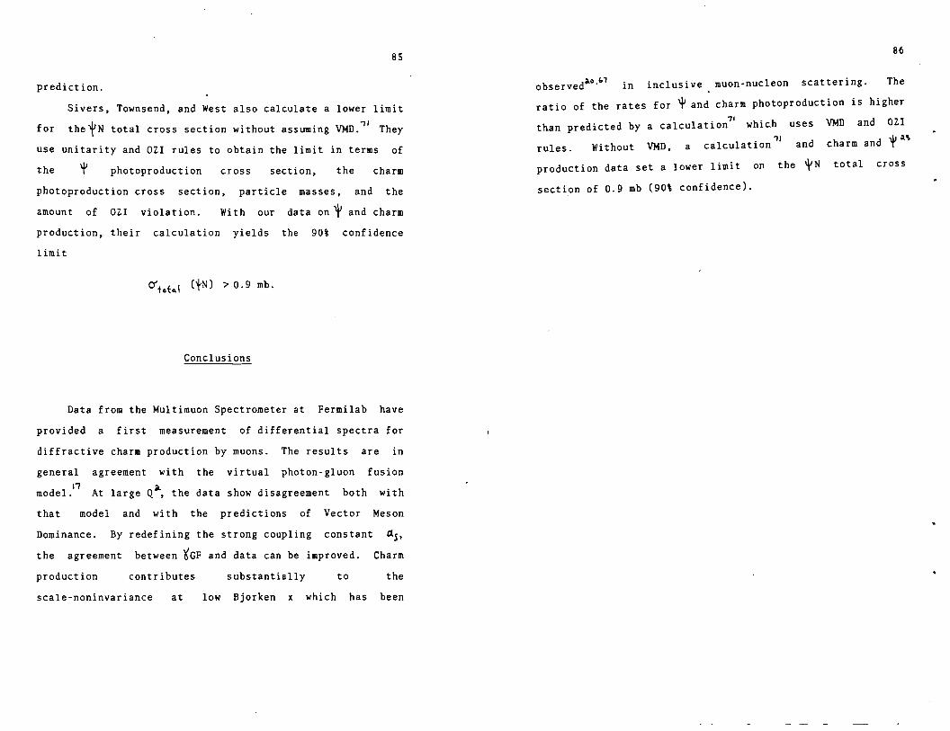
BS
prediction.
Sivers, Townsend, and West also calculate a lower limit
for thei'N total cross section without assuming VMD. 11 They
use unitarity and OZI rules to obtain the limit in terms of
the photoproduction cross section, the charm
photoproduction cross section, particle masses, and the
amount of OZI violation. With our data on 'Ji and charm
production, their calculation yields the 90\ confidence
limit
O"tot<>.I CtN) ":> 0.9 mb.
Conclusions
Data from the Multimuon Spectrometer at Fermilab have
provided a first measurement of differential spectra for
diffractive charm production by muons. The results are in
general agreement with the virtual photon-gluon fusion 17 a. model. At large Q , the data show disagreement both with
that model and with the predictions of Vector Meson
Dominance. By redefining the strong coupling constant a5,
the agreement between ~GF and data can be improved. Charm
production contributes substantially to the
scale-noninvariance at low Bjorken x which has been
86
observed-.0·"
1 in inclusive muon-nucleon scattering. The
ratio of the rates for '!i and charm photoproduction is higher 71
than predicted by a calculation which
rules. Without VMD, a calculation,,
uses
and
VMD and OZI
cha rm and '/! .a~
production data set a lower limit on the '¥N total cross
section of 0.9 mb (90\ confidence).
87
ACKNOWLEDGEMENTS
This experiment was performed by groups from Princeton,
Berkeley, and Fermilab. The Princeton group consisted of my
advisor, Frank Shoemaker, Pam Surko, and me. We were aided
by the mechanical expertise of Howard Edwards and other
technicians at the EP lab. Carl Bopp, Ann David, and Marius
Isaila labored with herculean fortitude to assemble our
drift chamber electronics. Al Clark, Karl Johnson, Roy
Kerth, Stew Loken, Tom Markiewicz, Peter Meyers, Wesley
Smith, Mark Strovink, and Bill Wenzel were the physicists in
the Berkeley contingent. Fred Goozen and other technicians
provided skilled technical support from LBL. John Caron
toiled arduously to create sophisticated analysis software
and Teri Martin tended the administrative fires in Berkeley.
Rol Johnson, Craig Moore, Marshall Mugge, and Bob Shafer
were in the Fermilab group. Garvie Hale's able assistance
at Fermilab was invaluable. I owe a substantial debt of
gratitude to all who worked on the muon experiment.
Dr. Yee Keung kindly gave me Monte Carlo generators
for charm and muon tridents and explained some of their
features. Professors Frank Merritt and Michael Shaevitz
willingly discussed shower Monte Carlo simulations with me.
The high energy physics groups of the University of Chicago
graciously provided me with office space and transportation
88
between Hyde Park and Fermilab for the last year of my
graduate work.

Appendix A IEEE Tunsactions on Nuclear Sch:nce, Vol. NS- 26, No. l. Febr~r, 1979 . DRIFT CHAMJER SYSTD1 FOR A BICI! RA'n I:XPERIMIJ,"T
C. Collin, !i. V. lHUa, r. C. Shoemaker and 1. Surko
Department of Physics , Princeton Univeraity, Princeton, H. J. 08~40
A 1y11tem of 19 large drift chamber s hu bun built and used in an experiment in the FlUl. tllUOn be.am . The design of the chu:bers and electronics enabled the ay•tui to perform t.•ith incident particle rates of up to 107 · per 1econd.
IntroducticD
J. 111aanetiud iroD spectrODeter hu been built and used in a DJOD experi11ent, I203A/391, at Fermilab. The iron ii in modules separated by 10 inch gaps in t.•hich are loceted the track charobers . Iach aap has a mult.it.•ire proportional ch&111ber t.•ith horizontal, vertical, 6.nd diaaonal cocrdin•tes read cut . The anode vires, t.•h ich 111eaaure the position of tracks 1D the bendin& (horizontal) plane, have 1/8 inch spacing.
To improve the resolution in the bendin& plane and to incre•H by redundanq the dficiency of detection, • sinale senu plane drift chamber vas included in each gap. The drift chamber's active aru is 42 x 72 inches. The left- right alllbiEU-itY in the drift ch&D1bera was to be resolved by track fittin& in the drift and multjvire ch~ere .
The iron iD the regjon between the chu.bera fonned a distributed taraet, ugnethed vertically t.·it.h a c;uite uniform fhl~. Since the bea= paue:d directly throu&h all of the chaaibe:n, the bum 111..1on's track could be tied to the final state :.uons ' tracks at the interaction vertex, lliproving the re:solution in mo:aeritu= a:od track angle. In addition, fin•l state trick.a frc1t cul ti-muoo events vhich lie in the beam region were not lost. !ecauu the drift cha1tbers had the intense bum and halo panins directly t hroush them, their delian vas somevhat different frDID that of IOIOSt chanber systems .
The expericent vu dui1ned for an incident muon flux (includin& the halo) of up to 10 7 per second . Therefore, a shorter t.han usual drift disunce was chosen to rr.inimhe the number of accidental tack1. tven so, a three prone event vould be expected to h1\:e T;\.;'O or three •ccidental tracks acco111panying it in the data rud out from the drift chambers . Because of this 1 the ch&Jllber system needed to be able to record more than one: hit per t.·ire per event 1 • The sense aepl1!ier-di1cri.ZOl.ina.tors \l'Ue built t.•ith a short dead t!me and the time di&ithin& system was designed t.•ith the ability to latch lllDre: than one signal per "·ire. \.11th thh multi ... hit c1pab1lity, the data could be plagued b)' false signals Nde: by straggl1n1 e:lectrons from ion pairs created aw•)' !roll! the: 111id plane of the cell . These electrons follow longer electric !ield lines to the senee \:ire. The drift cell (eo•ett')' \l'as chosen to e.ffectively itinimiz.e thia problem.
Cha11ober Design
The drift cells were constructed using graded potenti•h on the cathode ·t.·ires, sialilar to the sy1tem developed by Charpak2 . The cells ' di•endons •l•o
. Supported by the DepntJHnt of Eneru
Contract lrY-76-C-02-3072
wert: 1i•iln, except that the &axi•n11 drift distance "'•• choun to be 3/8 inch . Tbia VH • comproeiu beNeen the con of too m11ny channds and the problu of uceuive bukground tracka auoc1ated "'1th too long a •mory (drift) tiae: . \lith thh drift dhtance, the .. xi11U• drift tiiH: 01:1 the aid phne of the cell "·•• 175 ns . The spacing be~een the cathode ""ire planu ""•• l/4 inch. A thin chamber vith Cherpak'• acoaetr, bad"anu1eou1 if the electronics au dHi&ned "-1th aultihit capability in each channel, as it aini&hu the nu.her of late elect.ron1.
Tia . i. Schematic Diaaran of one Drift Ch.a•ber Cell
Fis . l. is a schf'..mstic dia&ram of one drift cell, showing the applied vol tage1 and the signal conne:ctions. Note th1t the four "'ires closest to the unae t.·ire on each side of the: chamber are conTM"cted toaecher to pr~ vide 1 ''clun" signal around reference . These eight "''ires, '11th the sense: wire, form• coaxial transmission line: with a characte.rhtic i•pedanc:e of about 400 ohu . The signal from •n eve:nt di"idu, half goina t010tard1 the sense attplifier, half goina in the opposite direction, tet.•ards the bottom of the chu:ber . The reflecticn of the latter from the end of the line t.·ould arrive at the amplifier too late: to be of u1e a nd could incruse the effective: dead-time of the se:nu aa:plifier. Therefore, the sense t.•ire h terainaud at the botton of the chamber . The cathode vire sy1t~ was biased at -100 volts to foni a clearing field vhich prevenu e:lectrons r eleased outside of the drift celh from cnterin& the cells and producinG late sigMll . lt:ithout thi• bias, the late electron sicnal was 60 per tent of the nusber of tracks through the chamber . \.'1th the bias
1 stras
gling electrons contributed leu than 1S% of the: rate . The lwer li•it on this contribution h uncertain since monte-carlo calcul•tions predicted that delta rays accompanying the 9.Jons \:ould produce about this rate of double hiu .
A plot of th«- electric field equirotentials iD a half cell, 1111de using conducting paptr 1 is shown in Fig . 2 . The sp1cin1 of the equipotentials h 167 volts. Note that the connection of four of the cathode t.·i res together did not. daNge: the ·ur.1fonity of the drift field . nie senie (anode) t.•iru \:Uc 20 sicron sold plated tungsten. The cathode t.•ires uere 100 r.icron silver plated beryllium copper . In tnta with ecdel chaabers, it was found that 50 aicron c.athode t.·ires produced field niuion •
U. S . Gove r n111ent work not protected by U.S. copyright.
> > > 0 9 ~ ~
f ~ i i
~ >
~
Tig. l .
~ ~ . . w
> > 0 0
~ ~
> > 0
~ .., 2
£q1.:ipotent!ah of the Ilectric Field in a Half Cell
In an iron spe:ctrouieter, ther~ h no need for thin chaa:ber "· in~ows, so the drift chacber s \l'e:re: built en 5/6 1nch thick s huu of duminul!! "tool snd ji&" plste:. tech plate '-'U 4 x 8 feet. This sir;pli!ie:d t he construction, and en1bled the active t.•idth of the chattber t o be a larger !uction of the space betveen the c.asnet coils th•n \l'Ould be the c••e if • heavy frame ue.re needed. The chat:bers t.•ere riounted "'1th the (lo"' Z) slu:.inuit plate up beaa !ro1r. the active volume: to reduce the nw:ober of delta rays. The do\."'Tl beani win~Ot."
\:'5S l/1.6 inch sluminum, prt'viding an iit"pen:1u.ble structure and ,col! shieldinb 1 as "'ell as a n equipotential for the clurina fie:ld .
Tis . 3. Chacber Construction Detail
Fig. 3 shovs the: vay the \Ji res t.•ere DOunted. They \l'ere soldued to pads fonr.ed by printeod circuit techniques on 1/8 inch thick G-10 6heets . After each plaoe was wound, the: next layer of r.- 10 '-"as epoxied in place . The t-:ylar cover in£ the solder pads on the bot toe l•yer of cathodet.·ires vas nE"eded to prevent dark current ftOtD ! lo"·ina to these p•ds . The sense t.•i res and ce:ll ed£e t.•ires vere hid by hend t'n precisely scribed lines. No c!Hficult)' veg found in replacing broken or =11- bid t.·ire:s - all that "as required '"as the re1r.cwal o! one or two of the cathode viru on the top plane. This con-1truction did initially cause probleu in the propu cleanina cl the vire: planCs. J. brush and 1olveni.1 , the usual chacber cleanin£ tool1 1 did not reach the bottOD cathode plane and as a result, the char:ibers had e:11ces-1ive noise rates. It was found, however , that squirtin& solver.ts onto the "·ires and blo.iing them dry with
nitrogen reduced the noise rate:s nearly to the calcuUted cosi:iic ray rate.
The: length of the sense t.·1ru , 72 inchu 1 h about the uximu• sta~le lensth for a safe ten~ion ob the 20 ~icron tungsten "'ire. To insure that the t.·ir es remined centered between the cathode phnu, bridses of C-10 were placed 12 inches on either side of the C!f:nter , dividing the chaJtibet into third1 . These constrained the cathoGc planes as "'ell as the sense plane, so that twists in the supporting alultinwr: plate would not influence the sp1t1n1. The space hetwten the G-10 strips on e1 ther side of the: sense plant ,.. .. deten:ined by the ce:ll edge t.•ires, so that the thinner sense viru \:ere free. To insure: thlit they did not hang up on the bridges, the challlbeu were pounded with • h&DDe.r as they hung wi tb the: wires vertical.
The , .. l.:'H sin:ilar to that uud by Chalr~k,2 approxiutely 2/3 argon , 1/3 ilobu tanc, exce:pt that the concentration of methy lal t.·as increased . During tuts on tr10del chnlbers, it t.·as found that an intense Rul06 beta gun could c;uickl)' deaden a section of • chacber unless the methylal content of the gas t.·11 sre•ter than in Ch1;rp5k's. Consequently, all of the argon '"as bubbl~d through methyld It o• C. There '-'U no degradation of the chambers' per fcn.ance caused by the intense muon bea11 ir. spite of the large currer.u (80 ~ per drift ch5cber) Cra.\."D dur!ns the spill.
Sense Amplifier - Dhcr!i::inator
The ser.e:e amplif1eu \:ere e:ach construc.ud of No Texas l nstTuMnts 10116 ICL inteirated circuits. These are triple differential line receivers 1.•i th d1f!uer.thl outputs . The ' 'oluge E•in hoc dU!nential ir.put to tiffue:nthl output h about 13 1 and the rise tiM is about 5 ns for sc.all siEnala anc! 2 ns for saturued si&nals. Fig . 4 shows the acplifhrs' scheoatic di5£r&C. Not shDI.~ ne pulld0t."n ru!stcrs betveen the amplifier outputs and ·5 volts on a ll su,es. The p\llldm.-n ru!stors .;ere 1500 ohms on all stages ncept the last , "'hich had 330 ohm resiuors.
°"' st .. u2j,_'_,-'oo-rr~ •l•f Cl
HI--+--+-'--< (,, .. 001--1,__..__,_.._-l
w1•u Cl 100
_,,
lOit l
"~~""... .. .... 100 C&tll
101tl
Tig .•• !:thematic Dia1u11 of the SenH AmplifierDiscriminator
To increase the. s1stem's COICllOn code noise i111t1Unitr, the acpl1f1er 1 s differential inputs were AC coupled to the cathode and sense t.'1 res of the drift chu:ber . AC coupling produced no problems because it "'U necessary tc.. clip the input pulses severely to r•duce the d.ad time: to acceptable levels. DTi!t chat:ber pulses typically ha\•e a length of 200 ns. The clippin& t.·u per-
• formt'd by 7.5 ns RC differentiation bett.•een the seccnd a nd third stages. It vas phced there to l\0 oid saturation of any amplifiers before t he clip, and to elicJ.nMe any difficulties due to 1>C offset of the: input ate&• ·

The input of the a.::1pl1f1er 'IJH protected by back-toback diodes. It is not kno1."D that they were needed. but there was ·no difficulty "'1th failure of inputs dcring the exper11:1ent. Note that the input has a high impedance (2000 ohms differential). This increased the r;ensitivity of the 51Dplifier by pulse-reflection doubling aod caused no difficulties becsuse the opposite end of the 1>e.nse vi re \.'86 terminated.
ThE sensitivity of the s.mplifier-discriU!inator \.>&S set by the 200 ttillivolt bia6 at the input to the third stage. The subu'!quent suges produced a utureted Ea. pulse '1."hich triggered the output stage through a 2 ns ti.JDe constant. The output "'"as connected as a one-shot (monostable) circuit "'hich produced a lS ns standard output pulse vith e dif!erentlll amplitude of &bout l.B vol ta.
The threshold sensitivity va1> 0.5 millivolu, t:ieasured 1.dth a signal \.'.'hich h11C a 200 ns decay timeconstant to Eit::Ulate drift ch&mber pulseE:. Th£ c3esd time, l!lasurecl at the end of the 200 foot ribbon cable, and dter the line receiver in the C1g1ti2.er, \:a& 35 The c11lcul&ted Efficiency, assut:ing 6 trs.cks in th£ c.hcmber, is thi=.n about 0. 98.
Time Digitizers
The digitiars Gesigned for this exp£ritcent follo-..•eC generiilly th£ logical systez:; "1.."hic"h Seuli 1 refers to as a Dig1tron 3 1.."ith "complete addreuing". A five-bit Cinary scaler is cepable of div::lc:!ing the drift ti::ie into 31 tilile bins, of about 7 m:nciseconds each. tiecause of the -multiple scettering in the iron, e finer subdivisien lJOi.:ld be pointless. '!his made possible. E.
relE.tivE-ly si:ple system, sho\."'n in Fig. 5.
fig, 5.
MASTER/SLAV[ f LIP -FLOPS
LOGIC TRUE
'I- Sil SMIF"T REGIS"l"EFI
~20 MHi
5- BIT BINARY SCALERS
Schematic Diagram of the Time Di ti tiz.er
The sigr • .a.ls frot:i the sense iimplifier~ 1Jere tr.ansir.itted .end delayed by ribbon cables about 200 feet long. The experiment's trigger logic produced a "pre-trigger1
'
'1.'h:ich \.'as used to init.iete the digitiz.ing process .and '"1'hich served as the timE re.ference. This :iniati:ted the delay required in the ribbon cables. If the fult. trig-
ger requirements turned o\lt to 'be uri.u.tisfied, the digiti:ters \Jere cleared, resulting in a deadtilDe of ooly 8
microsecond. The differential 6ignal from the ribbon cable 1..·as sc.plified by a 10115 clifferential line receiver. The resistor net\Oork .at the input terminated the ublE 1.nd provided 300 millivolts of fon.-srd biu, This ""as necesury because the 15 os pulses were attenu&ted much more by the cable than \JAS the DC level from the ECI. output. of the sense amplifier. The pre-trigger initiated the event ~ and the trein of 31 clock pulses. The digiti.z:ers accepted signds only for the duration of the event gete.
The dgns.l \:SS processed first by a T!r;ie Qucntizer!I which produced et it6 output the first clock pulse follo""1.ng the rising edge of the signal. This allowed all of the subsequent electronics to be ciesigned for synchronized signal6. Esch TitDe Quanti:ter \.'.1!16 cor.-str\lcted of No 10131 u:aster-slave D-type flip-flop1&." The outputs o! the 8 ti.Irie qc..enti:ters pessed vll &.b 8-1.1sy OR to e shift re&ister "·hich had its serial data input tied high. The first signcl to be rece.:l.ved therefore ce.used the Ollt.put Q0 of the shift regi5te.r to go high and this, in turn, latched the psttern of si&n£ls in that time bib end stopped the firi;;t scaler. The next sip·al frotll the s-·ay OR caused 01 of the shift register to go high, latching the pattun of signals in that time bin end stepping the seccnd scaler, etc. The shift register '"'as a hirc"hilO 10000, the scalers \.'er£ Fairchild 10016's "'"itl-, the fifth bit ;-ro,·ideC by s flip-flop iriven by the 10016 's fo"Urth bit. The lotches ...,ere 10153's. Not sho\."'Tl on the C.:l..s.grE..m is the delay in the sitn~ls bED-;een the Time Quanthers .and the l!!tches needed to synchronize them ""1th levels frot:. the shift register. Note th.at up to 4 of the 31 tilDE bins m2y be occup.:l.ed, end th.at ..any pattern of 6igm.ls on the B inputs "'i thin a t iwe bin i·s r i::corC.ed, \.".:i th one bit per channel. 'The trac:k efficiency of thic systt!lll is given by the formula:
""hEre UJ ... the nur.ber of active time bins • 21 p • the nwabu of bo.ards pE.r challlber ... 7 .t • the nur..ber of time slots per board • ~
the nuu.ber of trBcks per che:i!:bU.
For n • 6, the efficiency is 0.9985 for recording each track. The efficiency for recording 3 of the 6 tracks (ass"Ullling 3 £re background) is 0.995. The boards \,,lere cri&inally designed for & clock frequency of 150 ?-l::t and all \.le.re successfully tested at that fnquEncy, \.'hen the e..xperimer.t t.:as set up, however, tifficulties \."1th the clock fanout required the reduction to 120 ~z., so that t.he drift ti:me for the t::.ajor portion of the:. cell covered only 21 ti-me bins.
This formula for the efficiency assumes th.lit the tracks are di$tributed sutisticolly over the entire chac:.bt:r. This, of course, "'"a& not the cu;e - more ths.n hs.lf of them werE: in the beam region. To .evo::ld an overload of the digi t.i:ters connect.eel to the cells in the beam retion, a "ui.atrix box" \,,18S inserted ben;een the sense amplifiers ancl the cligitb.ers. This transposed the utrix of E:!ght atnplifier tDOdules each ""ith seven outputs to connect to seven digjth:ers each "·ith dght inputs. Thus the first digiti:ter board "·as ccmnected to the first, eithth, fifteenth, •.. cells, the second digit her board co the secon<!, ninth, •.• cells, etc. The intense beam region 'l.:'8S therefore distributed over ell of the digitizer boards.
In addition to the logic sho'l.-n on the diagram· overflo"\J& "'ere·recorded if more than 4 time bins v~re occupied. The ECL levels from the counters and latches were converted to TTL .end ...,e.re re.ad out Eerially into 8
FIFO regiEter, with empty d.ata '"'ords suppressed. This serial readout occurred ""hile the CAMAC systel!O was readint data from other parts of the e.xperiment so that no additional time ~as lost. The FIFO \JBS read out by the CA.MAC system. · .
The digitizers were congtructed on Hulti\.'.'ire5 circuit boards. The. conductors on these boards e.re r,3i; A't..'G insuleted copper ,_.ires "'hich ere laid by 11 co~putercontrolled machine in .e lay£r of epoxy ... ~hich covers a copper-clad C-10 printed circuit board. If the copper laye~ forms a continuous ground plane (interrupted only by su.s.l~ holes) tPen these conductors form good SO-ohm tr4".nsm.ission lines. There was no difficultv trans-cl t ting the 150 MH:t clock train on these boa~ds. The advantage of this construction is that the conductors ms.y cross \.l'ithout detectable cross-talk. The layout is therefore ve:ry much s!i:::pler than that of a printed circuit board. There is son.e cress-talk if conCuctors ha'l..·e long runs E.t the m1r.11'lum (0.05 inch) sp.;c:!.ng, but this. is euily svoideG. In the layout of the digitizers, care vas required to t:,.,;;tch the pinh lengths to keep the signels synchroni:ted. No di!ficlllty has been cbserved, ho,_;ever, due to lack of synchronization in the production beards.
The boards ""'en: rr.ount£-d in crstes \."hich servE:d No cha'Clbers each. The seven data-bo;i;rds for t:sch char:ber ~er.erE.ted 16-bit data 1..'Crds, each of ... +iich had e!rJbeOded in it a 3-bit bond address. A chamber-;;;dciress board for each chat::lbEr generated a. ...,ord containing chai:.ber number and cverflO'\J bits. This "·ere '"'as Cistinguishecl froci d.sta by an "illegEl" board adOress bit p.&.ttern. The ~ano~t. of the clock and £\"ent gate fer the seven boaras in each chon.ber group ""'as i;.lso performed on the chamber address bo.e:rd.
The principal diffici.;lty "'it.h this s)'He.I! during the experimer.t \.:BS 1.."ith the. mir,iature co.sxi.al cable conpectoris used fer the clock. \."'"hen tht:re vas an indic.:t!on of trouble, it usually coi.:ld be fixed by l.liggling the cables.
S'l.•s te!ll Perfon..enee
The operating sense "'ire voltage for the drift chambers \..•as chosen after investigcting the voltagE:c dependence of beth the eff:ic:.:l.ency and the resol\;tion. The ~fficiency, mEasured ""'it.h cos::ic rays and a p::..E.st:1c sc.intill.atcr telescope, typically plateaoed be.lo"· +1550 volts. The resolution, "Illes.sured in a small tut chclllber, did not reach its plateau until abciut +1700 volts. At this voltage, the ai::plification et the sense "'ire presumably ""as i;reat enough to place the signal from e single electron above the sense. amplifier-<liscri1dr.ator threshold. During the first part of the eY.periroer.t, the chat:ben l..'e!"e operated st +1800 volts. Later this
reduced to +1700 \'Olts to decrease the sisn5.l size into the sense srwplifiers, possibly reducing slightly the.ir dead time. The effect on the resolution anG Efficiency \.'B6 negligible.
The relationship bE:Neen drift time. .end clrift C.ists.nce is sho\lr'I in Fig. 6. The str&ight line is for reference only, to i;uide the eye. The 31 points "'ere obuined by integrating the population vs time bin histogram from a low intensity run "'ith strait,ht-throu!'.h triggers. The 2v~rege Ulwr.ination of the cells vas expected to be extremely uniform over the drift sp6 c:e. The histotraID had a t£11 "'•hich extended out to time bin· 31 although TDOSt of the hits fell in ti.me bins 3 through 23. This t.sil proC1..:ceCl the esymptotic approach of the
point& to the "Dli6.Ximum drift distance. That this was the correct ibterpretation \.>86 established by fitting data from beam tracks in five adjacent ch.e:::ibers t.:ith a parabola. Even small deviation& from this relationshi \.>OUened the x2 of the f1 t. p
.•OOr
l•oo "' u ~.zoo
.... "' c ~ •OO
~
c
rig. 6.
......
TIM[ BIN
Gnph of Drift Dist;rnce vs Time Bin Number
This asyttptor.ic approach to th£ ca:ximum drift distLnce is belie\.•ed to be due to the hct thct electrons free. trecks close to the cell eCge "ire, if f'Ot released ex~ctly .on the eid plane, have dgr.ificar.tly lonrer drift C1srar.ces ii.lcng the curved dectric field lines. There is probE.bly some ""'orsenir.g of the reEolut.ion in this region. The nonlinu.rity i~ teken ccre of in the tu.ck programs b;· si:r:ply using ~ look-up table coT1Uining '.H entries per chc"C'lbc.r gTOl.lp. tecause of some cable lengtt-, <i1fferences·, there are three gToups of chcrobers. The aver2t;e drift speed is 18 1tilS per time bin, or e.bou~.5.5 cm/i.Jsec.
The resolution cf the Grift chccbers while in place in the spectroJLeter 1..·as chedeC by the ofcre.centioned fjning prog:-ar.i. Since it \OC.S expected tliat there might be some c'l-.2mber construction errors, the chstiher rescluticn assumed in the program \.'"BS double that expected from the width of the ti1:1e bins, or 10 mils (250 :lticrons). The multiple scattering in the iron '"'as put in cuefully, including the correletions ben•een the s~attering offsets in adjacent c:h.e.mbeTs. The resulting X distributions wue narrower than that theoret:icc.lly expecteC, "but i..:i th a considerable teil. This is interpreted as sho ... ·ing that. the chacliers had clcEe to their ideal resolution. The tcil :!.!: believed to be due to delte r.eys ,,.·h;tch happen to prorluce iens closer to t'he sense 1."ire than the muon track. The trackfin~ing Frotratt now in use in the analysis of the experiment, \.""hich fits to both the drift ch.ambers and the 111ulth·ire proportionol ch.uibers, gi·ves a residual distribution for the drift c.h..aobers ._.i th a ....,id th of about 660 cicrons. This is largely due to c.ul tiple. sea tt£ring in the iron.
The chat::.ber hit efficiency, r:;easured "-!th non-ir.teracting beam muons, averagE'd be.tter th1in 98.5%. This efficiency 1..·as calculated frotll data taker, three c;uarters of t.he vay through the exp£ri11>er.t's run "'1th 8
muon beam containing ebout S. 5 x 10⁶ muons per spill \."1th additional muons in the halo. The full 1..·idth 2.t
half maximutn of this beat: \:es ten drift cells.
The noise rate for the OR of ell 56 chant1els in a chamber \."as· typically i; Utz. The rate exp~cted f!"oi:i cosmic ra~·s ... ·as ebout 1 k.Ez. Xo d.ar"k c\lrrent "'8S observed up to +2100 volts on the sense 1..·ire dllring these te&ts. Aftt:r the chambers 'Were :installed i 11 the

spectrometer, none bed a derk current above 300 pA, the miniln\.n:::i. observable. At the end of the experime.nt, after a total of I. x iol l J:DUons hed passed through the epectrometer "1'1th an average intensity of 5 x 10⁶ ·beam uruon.s per pulse, the dark current dra\.'"D. by one chamber vaa intermittently up to l lJA, "1'hile all of the othr1 re:Diaioed unobservable. This &hould be compared with the 80 µA
dr&wn. by e.ach chamber '*11le the bE.tni va1 passing through the i1.pp&ratus. Neither the ch.miber e.fficiency noL the resolution \,/ere observed to change apprec!.ably over· the course of the experiment.
Ackno"'·ledgement•
h'e vish to thank our collaborator• on this experiment, the me:mbers of the l....avrence Berkeley l.Aboratory and Fermilab groups, for their aissistance and support, The constrllction -of the chambers and the electronic Systems ,.,ere ebly performed by meni.ber& of our technical support group. \.'e vish to thank A. Y..ike Halling for hi&
help during· the ea:-ly parts of the development and in-1ull•tion of the equipment.
Referencu
l. F. Saul1, "Comments on Some :Proposed Sc.hemes for Drift Chamber Electronic&", CD.N NP Internal '.Report 73-12 (Rev.) (1973).
2. G. Cherpak, F. Seuli ·and lo:. Duinker, "High-Accuracy Drift Cha1Dbe.rs end Their U1e in Strong Magnetic Field&", Nucl. Inatr • .e.nd Meth., 108, lil3-A26 (1973).
3. I. Pizer, "A Multi~hannel !ime Recorder''. NP Internal Report 73-14 (1973).
li. Suggested by A. R. Clark, Private Ccmunication.
5. Y..anufectured by Photocirc\liU Division, Kollmorget1 Corp.,· Clen Cove., N. Y. ·

94
APPENDIX B
THE TURBO-ENCABULATOR*
For a number of years work has been proceeding in order
to bring to perfection the crudely-conceived idea of a
machine that would not only supply inverse reactive current
for use in unilateral phase detractors, but would also be
capable of automatically synchronizing cardinal
Such a machine is the "Turbo-Encabulator."
grammeters.
The only new
principle involved is that instead of power being generated
by the relative motion of conductors and fluxes, it is
produced by the modial interaction of magnetoreluctance and
capacitive directance.
The original machine had a base-plate of prefabulated
amulite, surmounted by a malleable quasiboscular casing in
such a way that the two spurving bearings were in a direct
line with the pentametric fan. The latter consisted simply
of six hydrocoptic marzlevanes, so fitted to the ambifacient
lunar waneshaft that side fumbling was effectively
prevented. The main winding was of normal lotus-0-delta
type placed in panendermic semi-boloid slots in the stator,
every seventh conductor being connected by a non-reversible
95
tremic pipe to the differential girdle spring on the up end
of the grammeters.
Forty-one manestically spaced grouting brushes were
arranged to feed into the rotor slip-stream a mixture of
high S-value phenylhydrobenzamine and five per cent
reminative tetraliodohexamine. Both of these liquids have
specific periosities of 2.SCn where n is the diathetical
evolute of retrograde kinetic phase disposition and C is
Cholmondoley's annular grillage coefficient. Initially, n
was measured with the aid of a metapolar refractive
pelfrometer (for a description of this ingenious instrument
see L. F. Rumpelverstein, Z. Electrotechnischtratishce
donnerblitze III, 212 (1929)), but up to the present date
nothing has been found to equal the transcending missive
dados cope. (See H. Feducc i et al. , Proc. Peruv. Ac ad.
Scat. Sci. ~. 187 (1979)).
Mechanical engineers will appreciate the difficulty of
nubing together a metahesive purwell and a superamitive
wannelsprocket. Indeed this proved to be a stumbling block
to further development until, in 1952, it was found that the
use of anhydrous nagling pins enabled a dryptonastic boiling
shim to be tankered to the bendyles.
The early attempts to construct a sufficiently stable
spiral decommutator failed largely because of a lack of
appreciation of the large quasi-piestic stress in the
sembling studs; the latter were specifically designed to

96
hold the tremic pipes to th~ spanshaft. When, however, it
was discovered that wending could be prevented by a simple
recession of the lipping sockets, almost perfect running was
secured.
The operating point is maintained as near as possible
to the h.f. rem. peak by constantly fretting the
anthragenous spandrels. This is a distinct advance on the
standard nivelsheave in that no additional dramcock oil is
required after the phase detractors have remissed.
Undoubtedly, the Turbo-Encabulator has now reached a
very high level of technical development. It has been shown
that it may successfully be used for encabulating nofer
trunnions. In addition, whenever a barescent skor motion is
required, it may be employed in conjunction with a drawn
reciprocating dingle arm to reduce sinusoidal depleneration.
The future promises frogs, dogs, and television sets.
*Based on a lecture delivered to Physics 1 by P.G. Bamberg,
Jr., Harvard University, Cambridge, Massachusetts, 1974.
97
REFERENCES
1. E. Fermi (1949).
and C. N. Yang, Phys. Rev. 76, 1739
2. S. Sakata, Prog. Theor. Phys . .!..§_, 686 (1956).
3. K. Matumoto, Prog. Theor. Phys. .!..§_, 583 (1956).
4. See, for example, M. Gell-Mann, Phys Rev. _!1i, 1067 (1962).
5. M. Gell-Mann, Phys. Lett. !• 214 (1964).
6. O. W. Greenberg, Phys. Rev. Lett. _!l, 598 (1964).
7. S. D. Drell and T.-M. Yan, Phys. Rev. Lett. ~.
316 (1970).
8. See, for example, K. J. Anderson et al.' Phys. Rev. Lett. ~. 944 (1979).
9. B. J. Bjerken and S. L. Glashow, Phys. Lett . .!..!.• 255 (1964).
10. S. L. Glashow, J. Iliopoulos, and L. Maiani, Phys. Rev. D2, 1285 (1970).
11. J. J. Aubert et al., (1974); J.-E. Augustin ~. 1406 (1974).
12. G. Goldhaber et al., (1976); I. Peruzzi et 569 (1976).
Phys. Rev. Lett. 33, 1404 et al., Phys. Rev:-Lett.
Phys. Rev. Lett. 37, al., Phys. Rev. Lett.
255 iZ_,
· 13. G. J. Feldman et al., Phys. Rev. Lett. ~. 1313 (1977).
14. R. Brandelik et al., Z. Physik Cl, 233 (1979).
15. See, for example, J. Kirkby in Proc. IX Int. Symp. on Lepton and Photon Interactions at High Energy (Batavia, 1979).
16. J. P. Leveille, University of Wisconsin Report No. C00-881-120 (1979).
17. See, for example, J. P. Leveille and T. Weiler,
..

98
Nucl. Phys. Bl47, .147 (1979), and references cited therin.
18. A.R. Clark et al., Phys. (1980).
Rev. Lett. ~. 682
19. A.R. Clark et al., Lawrence Berkeley Laboratory Report No. LBL- 10879 (to be published).
20. B.A. Gordon et al.' Phys. Rev. D20, 2645 (1979).
21. G. Goll in (1979).
et al., IEEE Trans. Nuc. Sci. NS-26, 59
2 2. V. Barger, w. Y. Keunf, and R. J. N. Phi 11 ips, Phys. Lett. 91B, 253 1980).
23. A. R. Clark (1979).
et al., Phys. Rev. Lett. ~. 187
24. W. R. Ditzler et al., Phys. Lett. 57B, 201 (1975).
25. See, for example, A. Silverman, in Proc. Int. Symp. on Electron and Photon Interactions at High Energies (Daresbury, 1969), Table 2.
26. P. A. Rapidis et al., Phys. Lett. 84B, 507 (1979).
27. The decay matrix elements of I. Hinchcliffe and C. H. Llewellyn Smith, Nucl. Phys. Bll4, 45 (1976) are used to describe D decay.
28. J. Kirkby in Proc. IX Int. Symp. on Lepton and Photon Interactions at High Energy (Batavia, 1979); M. Coles, private communication. Our experiment measures the product of the cross section and the average yield of muons.
29. W.A. Loomis et al., Phys. Rev. Dl9, 2543 (1979).
30. J. Proudfoot, Ph.D. Thesis, University of Oxford, 1978 (unpublished).
31. P. Bo set ti et al., Nucl. Phys. B54, 141 (1973).
32. P. Bo set ti et al. , Nucl. Phys. B60, 307 (1973).
33. G.A. Akopdjanov (1974).
et al., Nucl. Phys. B75, 401
34. w. Morris et al., Phys. Lett. 56B, 395 (1975).
99
35. E.L. Berger et al., Nucl. Phys. B77, 365 (1974).
36. v.v. Ammosov et al., Nucl. Phys. B58, 77 (1973).
37. S.L. Stone et al., Nucl. Phys. B32, 19 (1971).
38. R. Barloutaud et al., Sov. J. Nucl. Phys., 24, 303 (1976).
39. A. Bialas in Proc. First Workshop on Ultrarelativistic Nuclear Collisions, Lawrence Berkeley Laboratory Report No. LBL-8957 (1979).
40. A. Bialas and E. Bialas, Phys. (1980).
Rev. D21, 675
41. S.P. Denisov et al., Phys. Lett. 36B, 415 (1971).
42. S.P. Denisov et al., Nucl. Phys. B65, 1 (1973).
43. A.S. Carroll et al., Phys. Rev. Lett. ~. 932 (1974).
44. W. Galbraith et al., Phys. Rev. ~. 913 (1965).
45. J.E. Elias et al., Fermilab Report No. FERMILAB-Pub- 79/47-EXP 7185.178 (1979).
46. J.A. Gaidos et al., Nucl. Phys. B32, 10 (1971).
47. S.C. Loken, private communication. The correction is a hand fit to SLAC data comparing electron-neutron and electron-proton scattering.
48. D.H. Perkins, Introduction to High Energy Physics, Addison-Wesley, Reading, ~assachusetts, 1972, p. 40.
49. M. Shaevitz, private communication. Prompt muons from hadronic showers contribute less than 10% of the total muon yield.
50. W.A. Loomis, private communication.
51. C. Bricman et al., Review of Particle Properties, Lawrence Berkeley---raDoratory, Berkeley, 1978, p. 34.
52. See, for example, J.F. Martin et al., Phys. Rev. D20, 5 (1979). This experiment used 20.5 GeV electrons at SLAC.
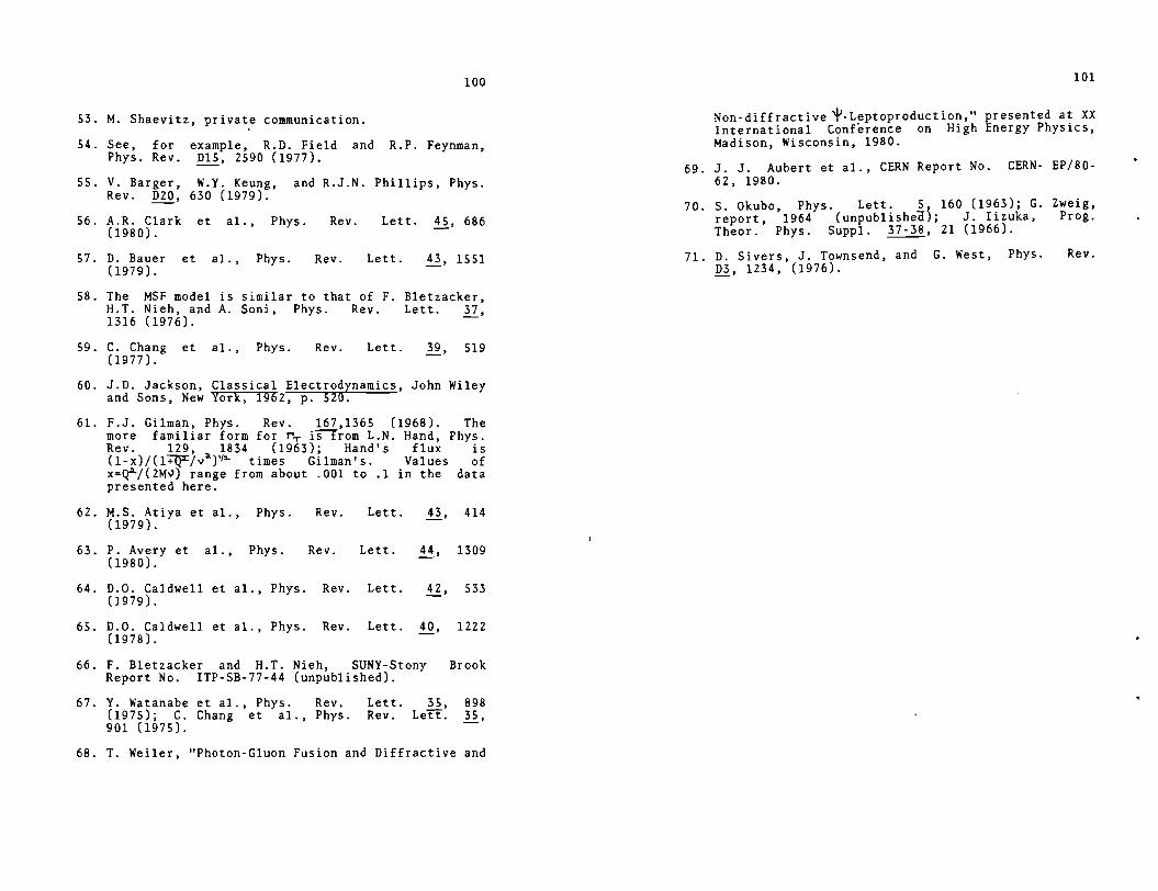
100
S3. M. Shaevitz, private communication.
S4. See, for example, R.D. Field and R.P. Feynman, (1977). Phys. Rev. DlS, 2S90
SS. V. Barger, W.Y. Keung, and R.J.N. Phillips, Phys. Rev. 020, 630 (1979).
S6. A.R. Clark et al., Phys. Rev. Lett. ~. 686 (1980).
S7. D. Bauer et al.• (1979).
Phys. Rev. Lett. 43, lSSl
S8. The MSF model is similar to that of F. Bletzacker, H.T. Nieh, and A. Soni, Phys. Rev. Lett. ~.
1316 (1976).
S9. C. Chang et al., Phys. (1977).
Rev. Lett. 39, Sl9
60. J.D. Jackson, Classical Electrodynamics, John Wiley and Sons, New York, 1962, p. 520.
61. F.J. Gilman, Phys. Rev. 167,136S (1968). more familiar form for rT i""Strom L.N. Hand, Rev. 129, 1834 (1963); Hand's flux (1-x)/(l+"Q=L/v")'1"- times Gilman's. Values x=Q4/(2M~) range from about .001 to .1 in the presented here.
The Phys.
is of
data
62. M.S. Atiya et al., Phys. (1979).
Rev. Lett. ~. 414
63. P. Avery et al., Phys. (1980).
64. D.O. Caldwell et al.• Phys. (1979).
6S. D.O. Caldwell (1978).
et al.• Phys.
Rev. Lett. ~. 1309
Rev. Lett. ~. S33
Rev. Lett. 40, 1222
66. F. Bletzacker and H.T. Nieh, SONY-Stony Brook Report No. ITP-SB-77-44 (unpublished).
67. Y. Watanabe et al., Phys. Rev. Lett. 3S, 898 (197S); c. Chang et al.• Phys. Rev. Lett. ~. 901 (197S).
68. T. Weiler, "Photon-Gluon Fusion and Diffractive and
101
Non-diffractive '\'-Leptoproduction," presented at XX International Conference on High Energy Physics, Madison, Wisconsin, 1980.
69. J. J. Aubert et al., CERN Report No. CERN- EP/80-62, 1980.
70. S. Okubo, Phys. Lett. S, 160 (1963); G. Zweig, report, 1964 (unpublishea); J. Iizuka, Prog. Theor. Phys. Suppl. 37-38, 21 (1966).
71. D. Sivers, J. Townsend, and G. West, Phys. Rev. 03. 1234, (1976).

102
TABLE 1
Calorimeter and hodoscope subtrigger combinations
resulting in a full dimuon trigger. Cluster 1 includes
calorimeter counters in modules 1 and 2, cluster 2 includes
modules 2 and 3, etc. as described in the text. Hodoscope
group 1 includes trigger banks 1, 2, and 3, placed after
modules 4, 6, and 8, group 2 includes trigger banks 2, 3,
and 4 after modules 6, 8, 10, etc.
1 2 3 4 5 6
Calorimeter cluster with subtrigger
(and any others downstream) (and any others downstream) (and any others downstream) (and any others downstream) (and 6 if present)
Required hodoscope groups with subtrigger
any of 1-6 any of 2-6 any of 3-6 any of 4-6 5 or 6 6
103
TABLE 2
Mean values of six reconstructed kinematic quantities
for data before background subtraction, for charm Monte
Carlo, and for Tf, K-decay Monte Carlo. All events have
E(daughter /A-) '> 15 GeV, v '> 7 5 GeV, and satisfy the standard
analysis cuts described in chapter III. Statistical errors
are shown.
Reconstructed kinematic Data Monte Carlo quantity Charm -rr. K
<\)) (GeV) 132.2 136.1 120.4 +0.2 +0.3 +1. 0
Geometric mean Q:i.. 0.547 0.729 0.260 (GeV/c)"- +0.004 +0.006 +0.011
< Dau~hter ,.._ energy) 26.02 26.35 23.58 (GeV +0.07 +0.08 +O. 21
<Inelasticity) 0.794 0.800 0. 793 +0.001 +0.001 +0.003
<Missing energy) 15.65 14.59 4.45 (GeV) +0.14 +0.18 +0.53
(p(daurter hto ~v) 0.749 0.676 0.618 (GeV/c +0.003 +0.003 +0.008
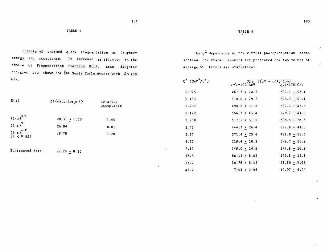
104
TABLE 3
Effects of charmed quark fragmentation on daughter
energy and acceptance. To increase sensitivity to the
choice of fragmentation function D(z), mean daughter
energies are shown for tGF Monte Carlo events with V> 150
GeV.
D(z) <EC daughter f<)) Relative acceptance
o.q (1-z) 28.31 + 0.15 1. 00
'l (1-z) 26.94 0.81
-l·S (1-z) 29.78 1. 20 ( z ( 0.99)
Subtracted data 28.20 + 0.20
105
TABLE 4
The Q1 dependence of the virtual photoproduction cross
section for charm. Results are presented for two values of
average v. Errors are statistical.
Q-. (GeV''/ca) O'eff ( ¥vN -- cC:X) (nb) 0)=100 GeV <:v)=l78 GeV
0.075 467.3 + 24.7 627.1 + 53.1 -0.133 518.6 + 29.7 628.7 + 55.1
0.237 498.3 + 31. 8 687.7 + 47.6
0.422 556.7 + 45. 4 720. 7 + 41. 5 - -0.750 517.5 + 31. 0 698.5 + 28.8
1. 33 444.3 + 26.4 588.8 + 41. 0
2.37 371. 4 + 23.4 488.0 + 19.6 -4.22 219.4 + 18.5 378.7 + 20.8 -7.50 149.0 + 14.1 274.8 + 16.8 - -13. 3 86.12 + 8.63 149.8 + 12.5
23.7 30.76 + 5.43 68.50 + 9.63
42.2 7.94 + 2.96 19.97 + 6.04

106
TABLE 5
The v dependence of the virtual photoproduction cross ;i._ ~
section for charm in the range .32 < Q < 1.8 (GeV/c) . The
first error shown is statistical, the second systematic.
'V (GeV) <rt.H (~vN __.. cC:X) (nb)
60.4 378.8 + 162.6 + 289. - 291.
69.8 393.9 + 102.0 + 189. - 187.
80.6 408.7 + 53.31 + 112. - - 106.
93.1 424.4 + 40.56 + 65. - 76.
107. 631. 8 + 41.53 + 36. - 30. -
124. 559.0 + 27.31 + 61. - 14.
143. 606.7 + 29.51 + 97. - 34.
165. 641.1 + 30.67 + 130. - - 49.
191. 693.1 + 44.68 + 162. - 60. -
107
TABLE 6
The Q~ dependence of the charm structure function F;i.Ccc) for
two values of average v. The first error shown is statistical,
the second systematic.
Q'J.. ;I.
(GeV/c) <'.v)=lOO GeV F ;i.. ( cC.)
<v> =178 GeV
0.075 (3 . 0 0 2 + 0 . 15 9 + 0 . 4 51 _4 ( 3 . 516 :_ O . 2 9 7 + 0 . 2 91 -~
-0.63l)x10 -0.222)x10
0.133 (6.117 +0.351 +0.513 -· (7.221 +0.633 +0.778 -4 -0.513)x10 -0.888)xl0
0.237 (10.69 +0.683 +0.641 -· (15.48 +1.07 +2.28 -~ -1.20)xl0 -1.15)x10
0.422 (21.60 +1.76 +2.48 ~ (30.99 +1.78 +1.21 ~ -3.07)x10 -2.ll)xlO
0.750 (36.08 +2.16 +2.86 ·• (55.89 +2.30 +Z.65 _11 -4.95)xl0 -4.55)x10
1. 33 (55.27 +3.28 +3.24 -~ (84.93 +5.91 +4.38 -~ -3.50)xl0 -7.00)xlO
2.37 (81.86 +5.16 +10.4 -4 (123.1 +4.93 +7.48 -~ -3.83)xl0 -3.40)xl0
4.22 (85.32 +7.21 +8.26 ~ (163.9 +9.01 +7.53 ~
-19.2)x10 -17.3)xl0
7. 50 (102.0 +9.62 +6.08 -- (203.0 +12.4 +12.2 -'( -10.5)xl0 -8.0l)xlO
13.3 (104.0 +10.4 +14.0 --1 (190.1 +15.9 +17.0 -o./ -7.lO)xlO -22.2)xl0
23.7 (65.60 +11.6 +2.76 -4 . (150.6 +21.2 +5.17 -'/ -28.4)xl0 -5.20)xl0
42.2 (29.94 +11.2 +1.17 -~ (76.78 +23.2 +23.7 -'i -1.71)xl0 -ll.9)xl0

108
TABLE 7
Calculated lO~d Fl. I d ln Q;i. at fixed Bjerken x vs. v
(top), Q~ (left margin), and x (diagonals, right margin).
For each Q2
-v combination, two values are shown. The bottom
value is fit to the structure function F2 for muon-nucleon
scattering (Ref. 20). The top value is the contribution
F2 (c') to F~ from diffractive muoproduction of bound and
unbound charmed quarks.
\l(Ge\I) 27 42 67 106 168
Q2 2
(GeV/c)
0.63
1.0
1.6
2.S
4.0
6.3
10
16
25
40
63
4 - 2 10 aF 2 (cc)ja.tnQ
l o4 aF 2 (µN) /d.tnQ2
17 30 43"' S4 S8 1070 ""-1090 ""-1110 1120 '-.....1130
23 43""' 63-..... 77......_ 84 980 '-.....1010 1040 '1oso '1060
30......_ s9'-..... 87"'-. io7'-...,. 116 6SO ........ 680 700 720 730
36-.... 73......_ 110-..... 139-..... 146 310 ......... 340 ........ 3SO ........ 360 ........ 360
36 80 128-..... 162....._ 163 320"' 390"' 430 ........ 460 ........ 480
29 75......_ 128-..... 165-..... 1S4 210 '-...,. 330 ........ 410 ........ 460 ........ 490
is, S4-..... 104"'-. 138"'-. i12 so ........ 220 ........ 340 430 480
4 -130
27-..... 64....... 90-..... S2 50 ........ 230 ........ 360 ........ 440
-2 7 -189 -126
0 -1 6 -31 -171 -122
10"' -22 so 240
0 l l -16 -23 -1S4 -119 so

110
Figure 1.-- Drell-Yan production of muon pairs through
quark-antiquark annihilation.
c: 0 Q)
(...)
:::J :z
c: 0 Cl>
(...)
::> :z

112
Figure 2.-- Models for charmed particle production.
(a) charmed sea production; (b) vector-meson dominance
production; (c) virt_ual photon-gluon-fusion production.
c
fL
N
11 '3
----------fL
c (a)
) charm
(b) ] x
fL a
cc
as N
(c)
Figure 2.

114
Figure 3.-- The Nl beam line at Fermilab. North is
towards the bottom of the page and west is towards the
right. Magnets Dl and QZ are in enclosure 100, Q~ and DZ in
enclosure 101, and D3 in enclosure 102. Q4 is in enclosure
103 and D4 is in enclosure 104.
t Ex1rac1ion -1200m
+ -soom D~cay
Vacuum
+ I -400m
Decay Vacuum
I
T -140m
1
x
zl t ·Proton
0 Target §"§:J QI
Triplet
I I I I I I I I I I I I I 1------Bm I
I I I I
~
(Nol To Scole l
Beam
Train
02
Con1air.s CH 2 Absorber
Q4
Neutrino Beam
J Moo" CCM Laboratory
Figure 3.
y
zl t. Proton Beam
x Target + /\Triplet
~Q2
T
8 a3
\I
Train
i::i Absorber
/\ 604
v

Quadrupole Magnet
Dipole Magnets
BH(x)
tn n ..... :;i .... ..... 'Tl ..... .... . ..... OQ Ill c: .... .... ..... C1I 0 :;i ... n 0 c: :;i .... C1I 3: .... c: tn ..... .... ..... ..... ;:l ~ ..... .... .... ::r C1I C1I
51 c: 'O 0 .... :;i 0
'O O" 0 C1I .... Ill .... a .....
0 :;i Ill .....
n ::r Ill 51 O" C1I .... tn
Ill :;i
"'
BH (x,y) MWPC
BH(x,y) MWPC Vh MWPC
Yj
BH Beam scintillator holoscope Vj "Jaw" veto counter
Yw Large veto wall Vh Halo veto hodoscopc
BH(x,y)
vb Bucket occupancy veto counter MMS Mullimuon Speclromcler CCM Chicago Cyclotron Magnet
Figure 4
..... ..... Q\

ll8
Figure 5.-- The Multimuon Spectrometer. The magnet,
serving also as target and hadron absorber, reaches 19.7
kGauss within a l.8xlxl6 3 m fiducial volume. Over the
'3 central l.4xlxl6 m , the magnetic field is uniform to 3% and
mapped to 0.2%. Eighteen pairs of multiwire proportional
(MWPC) and drift chambers (DC), fully sensitive over l.8xl
m~, determine muon momenta typically to 8%. The MWPC's
register coordinates at 30° and 90° to the bend direction by
means of 0.2 inch cathode strips. Banks of trigger
scintillators (S,-S, 2 ) occupy 8 of 18 magnet modules.
Interleaved with the 4-inch thick magnet plates in modules
1-15 are 75 calorimeter scintillators resolving hadron
energy E with
upstream of
rms uncertainty 1. SE 11a. (GeV). Not shown
module 1 are one MWPC and DC, 63 beam
scintillators, 8 beam MWPC's, and 94 scintillators sensitive
to accidental beam and halo muons.
MULTI-MUON SPECTROMETER
BERKELEY-FERMILAB-PRINCETON 9
in modules 4,6,8, 10, 12, 14, 16, 18
PC+ DC in 1-18 5C in 1-15
Figure 5.
"'
14
XBL 795-15:

120
Figure 6.-- One module in the muon spectrometer.
- - _J
CONCRETE BASE
Figure 6.
,~,
PROPORTIONAL CHAMBER
DRLFT CHAMBER
~c-'--- TRIGGER HOOOSCOPE
SUPPORT PLATE
. : . L __ _
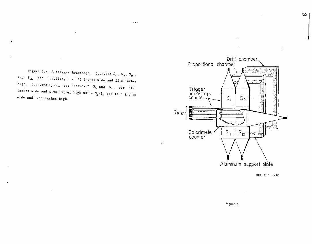
122
Figure 7.-- A trigger hodoscope. Counters S1
, S.;i_, S11
,
and S,;i. are "paddles," 20. 75 inches wide and 23.8 inches
high. Counters 53 -S, 0 are "staves." S'!> and S,0
are 41.5
inches wide and 5.98 inches high while ~ -~ are 41.5 inches
wide and 1.55 inches high.
Proportional
Trigger hocfoscope counters
Colorimeter counter
1~3
. '
Aluminum support plate
XBL 795-1602
Figure 7.

124
Figure 8.-- Calorimeter subtrigger patterns for dimuon
events. (a}
subtriggers.
scintillators
cluster grouping of counters; (b) examples of
Pulse heiJhts in at least five of ten
in a cluster must exceed a threshold for that
cluster to satisfy a calorimeter subtrigger.
-..c
(a)
2 3 15 16 Module
111~~11~ II 3 )\___]
1---~===-~-1 ~ ~~\l~---1 2 14
Colorimeter cluster
(b)
2 3 4 Module
1 \ 11. ---Threshold I I I II J..lliJ
Clusters 1 and 2 satisfy subtri gger
2 3 4 Module
i Jl ill _l :J
~Threshold
I II I I
a.. Cluster 1 satisfies subtrigger
Figure 8.
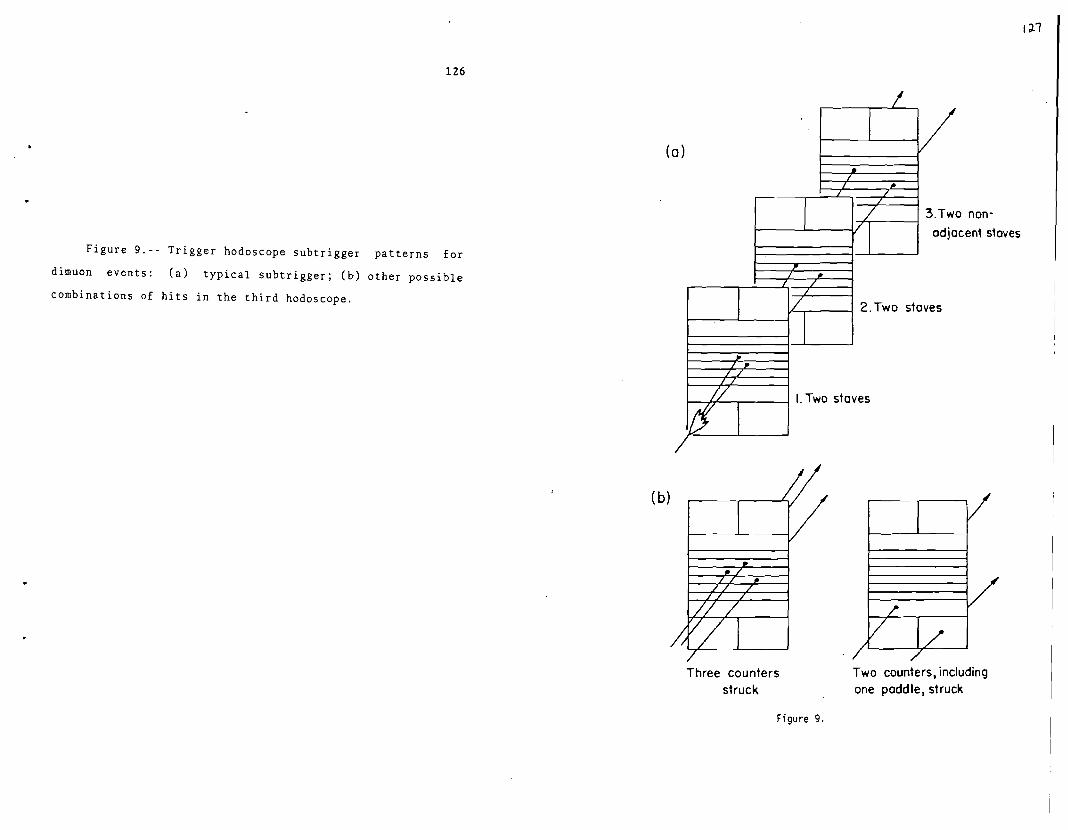
126
Figure 9.-- Trigger hodoscope subtrigger patterns for
dimuon events: (a) typical subtrigger; (b) other possible
combinations of hits in the third hodoscope.
(a)
( b)
.... ~---1 3.Two non-
adjacent stoves
2. Two stoves
I. Two stoves
Three counters struck
Figure 9.
Two counters, including one paddle, struck
t:2.1

Figure 10.-- Calorimeter
vs. shower energy.
128
subtrigger probability
:0 "' .0 0 ....
Q.
/ l 'l
..
0.00 -4<~~--,-~~----.~~~..-~~.-~~...,--~~.,~~~.-~~.-~~.-~~-r-
0 10 20 30 iO so 60 70 BO 50 100
Eshower (GeV)
Figure 10.

130
Figure 11. - - Multiwire proportional chamber
center-finding electronics.
..
MWPC Cathode amplifiers
\14MC10115P
Figure 11.
+
+ Output voltage
XBL 795-1599

132
Figure 12.-- A drift chamber cell and preamplifier.
The cathode wire spacing is 1/12 inch and the separation
between cathode planes is 1/4 inch. The full width of the
drift cell is 3/4 inch. In the circuit, each stage is
one-third of a 10116 ECL triple line receiver. Not shown in
the circuit diagram are "pull-down" resistors connecting
both outputs from each stage to -SV.
> 0 > 0 0
0 tD
I
• • -1600V e
• • > > 0 0 0 0 ~
-sv
> 0 0 tD
I
•
• > 8 tD
> > 0 0 0 Q <.!> I I • • • • • • ,,-+1750V
Sense Wire
t ' ' ' • > > 8 0
0 <.!>
Figure 12.
> 0 0
I
•
• > 0 Q
> 0 0 ~
I
• e-1600V
• > 0 0 <.!>
balanced ribbon coble
133
•

134
Figure 13.-- 'Logical" flow in the track-fitting program.
Fit tracks with MWPC's
only
Add DC's to t rocks
Remove hits to minimize x2• maximize hi ts
F wse broken tracks, discord stray tracks
Use tracks+ colorimeter to choose vertex
Refit tracks, including vertex
Remove hits to reduce
x2
Search grid for best vertex x,y,z
yes
Write tape and proceed to next event
Refit tracks, choose new vertex with 1rocks +colorimeter
A
Figure 13.
Ignore colorimeter information
Reinstate oil canceled
hits
Use only tracks to choose vertex
Refit tracks with vertex
Refit tracks including colorimeter information
Remove hits end refit tracks
Reject event ond proceed to next event
Discord colorimeter information
Use trockonly vertex

136
Figure 14.-- cc pair mass in the photon-gluon-fusion
model.
.,, ..... c: ::: >, I-
'° I-..... .J:> I-
'° lu u
E "'C ...... z "'C
1
10-! \
10-2
10-3 -1-~---r--r-----r-.----.-.---.-.--.-11-.-l--;-l---;->-l--r--
5 6 7 8 2 m - (GeV/c ) cc
Figure 14.
9

138
Figure 15. - - Momentum transfer-squared in the
photon-gluon-fusion model. (a) All events generated; (b)
Events satisfying the dimuon trigger.
"' ..... c: ::l
~
"' !.-..... 0.50
..0 !.-
"' (\J
0 "O ...... z "O
(\J
0
Figure 15.

llf-1
140
Figure 16.-- Hadronic shower energy in the
photon-gluon-fusion model. (a) All events generated; (b)
Events satisfying the dimuon trigger. ~
j "' +" ·~ c: :::i
>. r... "' r... +"
:0 0. 50 r...
"' r... Ill .. 0 .s: "' lg·
...... z: "C
,
Eshower. (GeV)
Figure 16.

142
energy in the Figure 1 7. - - Daughter muon
I
~ ~ I
10-l -J "' ....,
l c:
"" "'
(b) >, (a) '\ I-
' \ "' I-....,
\ .0 I-
"' ~ ::i
I-ClJ ...., i
..c:
w-2 j "" "' "' "'Cl w "'Cl ....... :z: "'Cl
photon-gluon-fusion model: (a) all events generated; (b)
events satisfying the dimuon trigger.
10 20 30 40 50 ED 70 80
Edaughter µ (GeV)
Figure 17.

144
Figure 18.-- Energy lost by the beam muon in the
photon-gluon-fusion model. (a) All events generated; (b)
Events satisfying the dimuon trigger.
Ill ..., c: ::>
t' io-1 "' I-...,
..c I-
"' ;>
" ....... z "
..
0 20 60 80 100 120 160 !BO 200
\) (GeV)
Figure 18.

146
Figure 19.-- Distribution of interaction vertices in l. 00 -1 L x
~ x slabs in a module for shower Monte Carlo events.
x ~ x ~
ro ~
0 ~
~
~ > ~
0.50 ro ~ ~
2 5
slab
Figure 19.

148
Figure 20.-- Distance from vertex to meson decay point
for shower Monte Carlo events. ~
"' ..., -~
c: ::i
t> "' .... ..., :c .... "' ~
.J: ..., "' 0. ...,
.J: O>
:;:: ~
-0 ........ z: -0
w-1
10-2
10-3
~ """
0 50 100 150 200 250 300 350 100 150
meson flight path (cm)
Figure 2·0.

150
Figure 21.-- Probability vs. shower energy for a > Cl.I
<.!:> shower to yield a decay muon with more than 9 GeV of energy.
"' "
;:J_ w
..c: .µ
3: ;:J_
"' c
"' .µ .CJ
,n-1 1 0 ·- -0 .µ
~ >, .µ
1 .CJ
"' .CJ 0 '-
0..
I
20 10 60 BO 100
Eshower (GeV)
Figure 21.
120 110 160
IS-I
I
iSO 200
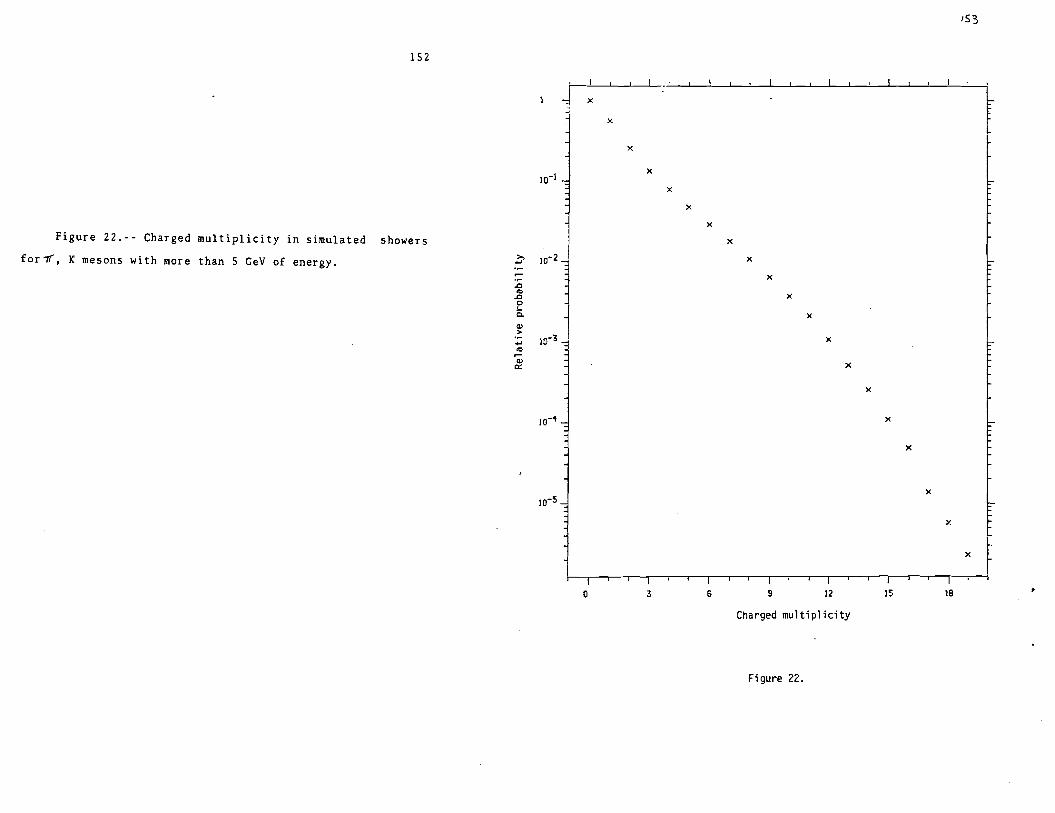
1S3
152
' ~ x f x
L x
10-l x
x
x
x Figure 2 2. - - Charged multi pl ici ty in simulated showers x
for-rl, K mesons with more than 5 GeV of energy. >, ..... w-2 x
x .0 ., .0 x 0
.,J s.. x Cl.
(I) >
x ..... ., ., ~ x 0::
x
10-1 x
x
x 10-S
x
x
0 3 6 9 12 15 18
Charged multiplicity
Figure 22.

154
Figure 23.-- Number of meson generations between
virtual photon-nucleon interaction and decay muon in >, ...,
simulated showers. .L:l
"' .L:l 0 .... Q.
QJ
> ..., "' QJ
0::
x
10-l
10-2
10-3
x
I
2
x
3
Number of meson generations
Figure 23.
x

156
Figure 24.-- Decay probability for '!'('•s and K's in
simulated showers.
"' ..... c:
"' >, .._
"' .._ ..... ..Cl .._
"' Q.,
" ...... ;z
" Q.,
, I ',I
1.00 ~
j 0.50 I
Decay probability P
Figure 24.

158
Figure 25.-- Energy lost by the beam muon in simulated
inelastic collisions.
V1 I0-1 .µ
c :::>
>, ,_ "' ,_ .µ
..c ,_ "' ;:>
"'C ..._ z: "'C
I0-2
0 20 60 BO JOO 120 110 160 180 200
v (GeV)
Figure 25.
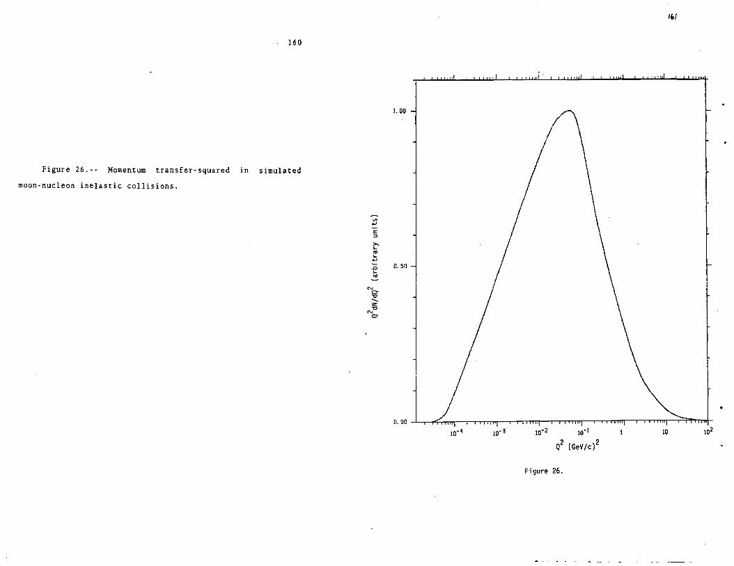
160
I. 00
Figure 26.-- Momentum transfer-squared in simulated
muon-nucleon inelastic collisions.
"' .... ·~ c: :::>
>, .... ro .... .... ·~ 0. Sil ..0 .... "'
N CT "'C ....... z "'C
N CT
I
~ ~
j
/\ I
10-2 w-1
Q2 (GeV/c) 2
Figure 26.
'"'
•
10
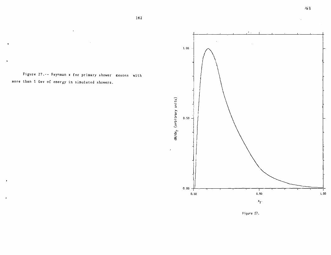
162
Figure 27.-- Feynman x for primary shower mesons with
more than 5 Gev of energy in simulated showers.
"' +'
c::
"' t' "' ... +' ·~
..0 ... "'
l.J... )(
"'C ...... z "'C
I. 00
11 ~I 0.50
j
0. 0(1 I
0.00
llO 3
\
\ \
o. so I. 00
Figure 27.

164
Figure 28.-- distributions for primary shower
mesons with more than 5 GeV of energy in simulated showers. rn-1
"' +'
c:
l ~
>, ... "' ... +' ~
.<:I ... "'
N f-c.
"'C 10-2 ......
;a
Figure 28.

166
I. CO 1 I
4
Figure 29.-- Feynman x distributions for all secondary I ~ ' l
I J
mesons before imposing energy conservation in simulated
showers.
I/) \ ..., \ c:
l ~
\ >, .... "' ....
0.50 I ..., .0 .... "' u.. I x
"O ...... :z: "O
0.00 o. 50 I. 00
Figure 29.

168
Figure 30.-- p~ distributions for all secondary mesons T
imposing energy conservation in simulated showers.
Vl .... <= ~
>, .... "' .... .... .0 .... "'
N I-
c. -0 ...... z -0
r .J
:J j J
,,
10-21
10-3
~
1 0
2
Figure 30.

170
Figure 31.-- Energy of hadrons which decay in simulated 10-l
showers.
"' ...., c: ::i
>, .... re .... ....,
..0 .... 10-2 re
c: 0 ....
"C re
.<::: LU "C ...... z "C
io-3
r
10 20 30
Ehadron (GeV)
Figure 31 .
llJ
so 60 70
r
r
80

172
Figure 32.-- Muon momentum along z axis for decay muon
from simulated showers.
"' 10-2 ..., c:
"' >, ... "' ... ..., :;; ... "'
N Cl.
10.-~
"'Cl ....... :z "'Cl
173
10 20 30 iO 50 60 70 80
Pz (GeV/c)
Figure 32.

174
Figure 33.-- Energy of produced muons for simulated
shower events satisfying the dimuon trigger. 10-l
"' ,.., c: :::>
>, .... "' .... ,..,
.a
I .... "'
;1 1 l.U "O ....... :z "O
10-2
0 10 20 30 ~D SD 60 70
E ( GeV) 11
Figure 33.

176
Figure 34.-- Momentum perpendicular to the virtual
photon for produced muons at the decay point in simulated
shower events satisfying the dimuon trigger.
"' ..... c: :::>
t' "' s.. ..... ·~ ..0 s..
"' I-
0. -0 ...... z: -0
111
10-I
10-2
0.00 1. 00 2.00
Pr (GeV/c)
Figure 34.

l iC
Figure 35.-- Neutrino energy for simulated shower
events satisfying the dirnuon trigger.
O.QO 12. 5 25. 0
E (GeV) v
Figure 35.

180
Figure 36.-- Feynman diagrams for muon trident SS"
production calculated by Barger, Keung, and Phillips. (a)
Bethe-Heitler production; (b) Muon bremsstrahlung; (c)
Target bremsstrahlung.
,.
(a) Bethe - Heitler
/-'- µ
fL
fL
l T T
( b) Muon- Bremsstrahlung
fL
(c) Target- Bremsstrahlung
fL fL fL
fL
fL
T T Figure 36.
1g1
fL
fL
fL
fL
fL
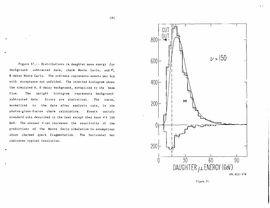
182
Figure 37.-- Distributions in daughter muon energy for
background- subtracted data, charm Monte Carlo, and?(,
K-decay Monte Carlo. The ordinate represents events per bin
with acceptance not unfolded. The inverted histogram shows
the simulated~. K-decay background, normalized to the beam
flux. The upright histogram represents background-
subtracted data. Errors are statistical. The curve,
normalized to the data after analysis cuts, is the
photon-gluon-fusion charm calculation. Events satisfy
standard cuts described in the text except they have v> 150
GeV. The unusual v cut increases the sensitivity of the
predictions of the Monte Carlo simulation to assumptions
about charmed quark fragmentation. The horizontal bar
indicates typical resolution.
800
600 v > 150
400
200 H
200
0 30 60 90 DAUGHTERµ ENERGY (GeV)
XBL 802-378
Figure 37.

184
Figure 38.-- Reconstructed vertex distribution for
background- subtracted data and charm Monte Carlo. Monte
Carlo events were generated only in the upstream -BOO cm of
the detector. (a) The histogram shows subtracted data with
Monte Carlo superimposed as x's; (b) The histogram shows
Monte Carlo with subtracted data superimposed as x's.
E u
.,.., <:t <:t ....... "' .µ c: QJ > CIJ
E u
.,.., <:t <:t ....... "' .µ c: QJ > QJ
zvertex (cm)
"
1000 ~
" Monte Carlo
0J1~~..,.-~-,--~--.-~--.~~,1~--.~--.~~.--~-.--~.,_ -40 560 1160
zvertex (cm)
Figure 38.

186
Figure 39.-- Distributions in daughter muon momentum
perpendicular to the virtual photon for background-
subtracted data, charm Monte Carlo, and 11', K-decay Monte
Carlo. The ordinate represents events per bin with
acceptance not unfolded. The inverted histogram shows the
simulated 1f, K-decay background, normalized to the beam
flux. The upright histogram represents background,
subtracted data. Errors are statistical. The curve,
normalized· to the data after analysis cuts, is the
photon-gluon-fusion charm calculation. Events satisfy
standard cuts described in the text. The horizontal bar
1600
1200
800
400
indicates typical resolution. 400
0 0.5 1.0 1.5 p (DAUGHTER µJ J_ TOrv (GeV/C)
XBLB02-3BI
Figure 39.

188
Figure 40.-- Distributions in energy . transfer for
background- subtracted data, charm Monte Carlo, and ff,
K-decay Monte Carlo. The ordinate represents events per bin
with acceptance not unfolded. The inverted histogram shows
the simulated ~. K-decay background, normalized to the beam
flux. The upright histogram represents backgrou0
nd-
subtracted data. Errors are statistical. The solid curve,
normalized to the data after analysis cuts, is the photon-
gluon- fusion charm calculation. The dashed curve
represents an alternative model in which DD pairs are
produced with a hard fragmentation function and a
probability independent of ~. Events satisfy standard cuts
described in th~ text except that no~ cut is imposed.
horizontal bar indicates typical resolution.
The
800
600
400
200
I
200
I I I
cuTj / OUT I I
II
I I
I I
50
A 11
/ I I I I I I
100 v(GeV)
Figure 40.
\
150
\ \ \ \ \ \ \ \ \ \ \ \ \
200
XBL 802-376
IB"I
• I

190
Figure 41.-· Distributions in momentum transfer-squared
for background- subtracted data, charm Monte Carlo, and Ti,
K-decay Monte Carlo. The ordinate represents events per bin
with acceptance not unfolded. The inverted histogram shows
the simulated 1f, K-decay background, normalized to the beam
flux. The upright histogram represents backgro~nd-
subtracted data. Errors are statistical. The curve,
normalized to the data after analysis cuts, is the photon-
gluon- fusion charm calculation. Events satisfy standard
cuts described in the text. The horizontal bars indicate
typical resolution.
800
600
400
200
200
0.1 I ( GeV/C)2
10
XBLB02-377
Figure 41.

192
Figure 42.-- Distributions in missing (neutrino) energy
for background- subtracted data, charm Monte Carlo, and 1f;
K-decay Monte Carlo. The ordinate represents events per bin
with acceptance not unfolded. The inverted histogram shows
the simulated 1f, K-decay background, normalized to the beam
flux. The upright histogram represents background-subtracted data. Errors are statistical. The curve,
normalized to the data after analysis cuts, is the photon-
gluon- fusion charm calculation. Events satisfy standard
cuts described in the text. The horizontal bar indicates
typical rms resolution. The arrow indicates the shift in
the centroid of the data caused by a +2.5\ change in the
calorimeter calibration.
l'l3
1500
..
1000
500
500 _80 -40 0 40 80 MISSING ENERGY (GeV)
• XBL802-380
Figure 42.
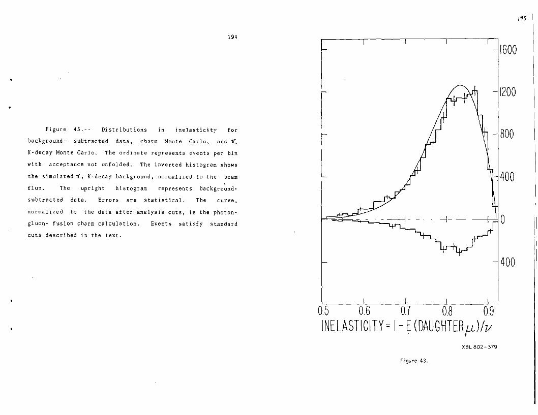
194
Figure 43.-- Distributions in inelasticity for
background- subtracted data, charm Monte Carlo, and 7f,
K-decay Monte Carlo. The ordinate represents events per bin
with acceptance not unfolded. The inverted histogram shows
the simulated~. K-decay background, normalized to the beam
flux. The upright histogram represents background-
subtracted data. Errors are statistical. The curve,
normalized to the data after analysis cuts, is the photon-
gluon- fusion charm calculation.
cuts described in the text.
Events satisfy standard
1600
1200
800
400
400
0.5 0.6 0.7 0.8 0.8 lNELASTlCITY =I E (DAUGHTERµ) Iv
XBL 802- 379
Figure 43.

196
Figure 44.-- Flux of transversely polarized virtual
photons accompanying a 209 GeV muon. The flux is in units ... -~ of c GeV and represents the number of photons per unit
interval of Q~ and~. Shown in the figure is Q~ times the
flux. I > ClJ
c.!l
l.Oxl0- 5
~ 7.5x10:-6 N
CT
5.0xl0- 6
1
I o. 1
Figure 44.
v=lOO GeV
v=l78 GeV
1~1
''I 10 100
•
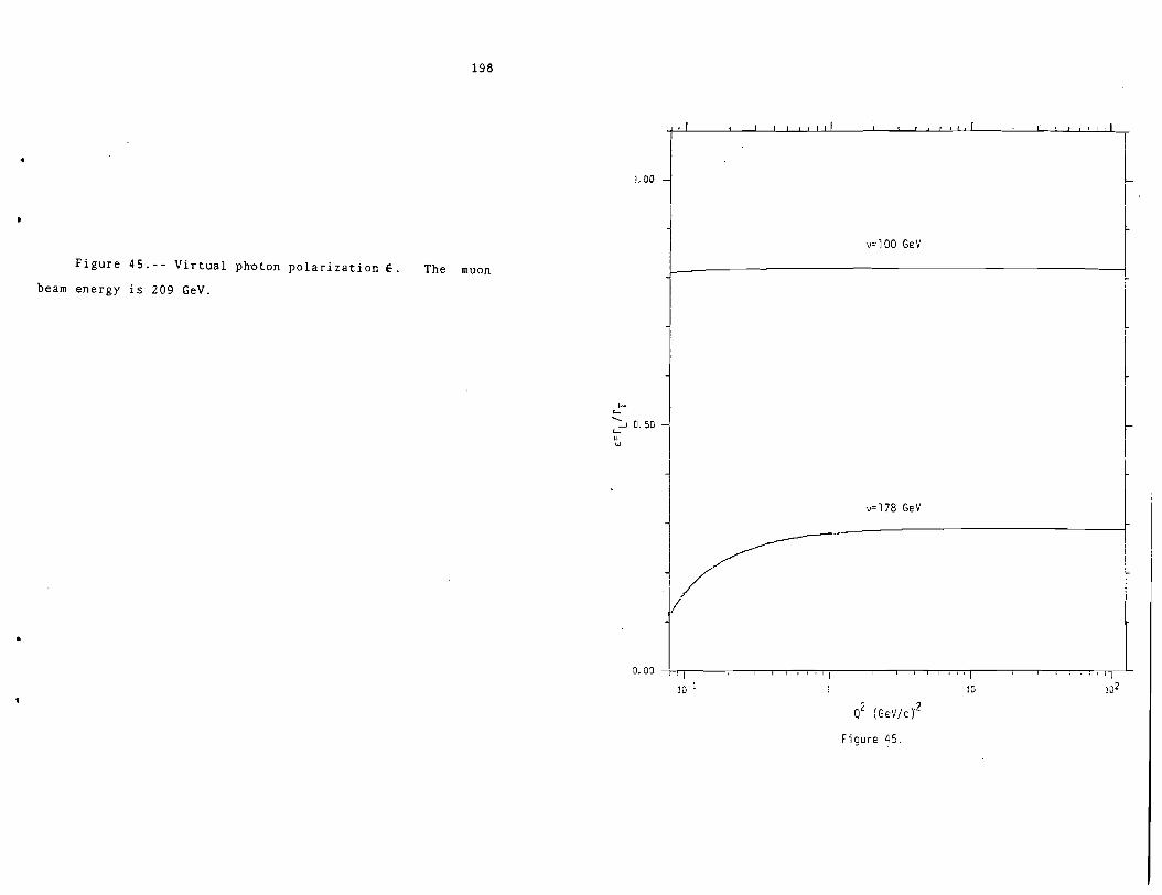
198
r 1 I I' t I 11 ( I l i I
I
l l. DO
I ~
r I v=lOO GeV I I Figure 45.-- Virtual photon polarization E. The muon
beam energy is 209 GeV.
>--'-
--:._, 0. SD -: t s I I I
I I
~
j v=l78 GeV
j i I L i
• 1/ r 0. OD --r-1 I 'I I I I I I I'!
10-l lD io2
02 (GeV/c)'2
Figure 45.
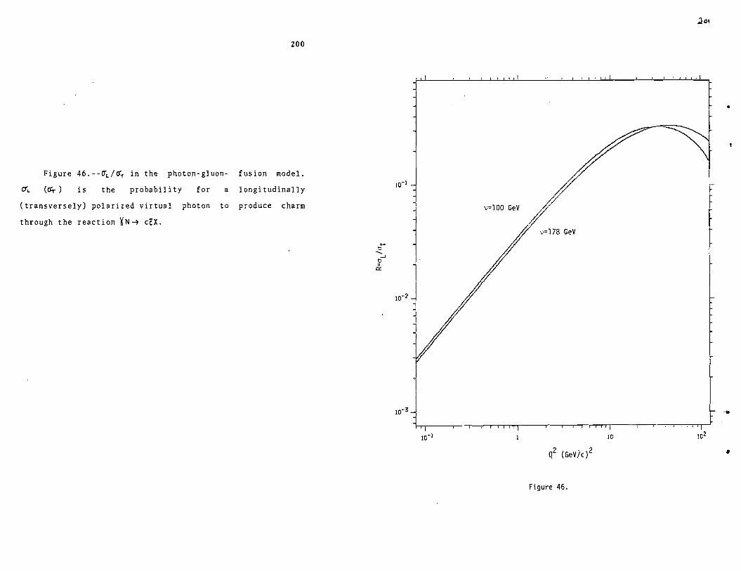
200
Figure 46.--~~/~T in the photon-gluon- fusion model.
is the probability
(transversely) polarized virtual
through the reaction ~N-t c(X.
for a longitudinally
photon to produce charm
ti ....... ....J
b II er:
' I
v=lOO GeV
v=l78 GeV
..
•
Figure 46.

•
202
Figure 47.-- fR in the photon-gluon-fusion model. R is
~ /~ ; € is the virtual photon polarization (see figures 45
and 46).
lb I-
'...._ _J
t: _J
'-II
c:< w
' , I
J v=lOO GeV I
/] / l
v= 178 GeV / w'~ /
~ / l/
Figure 47.
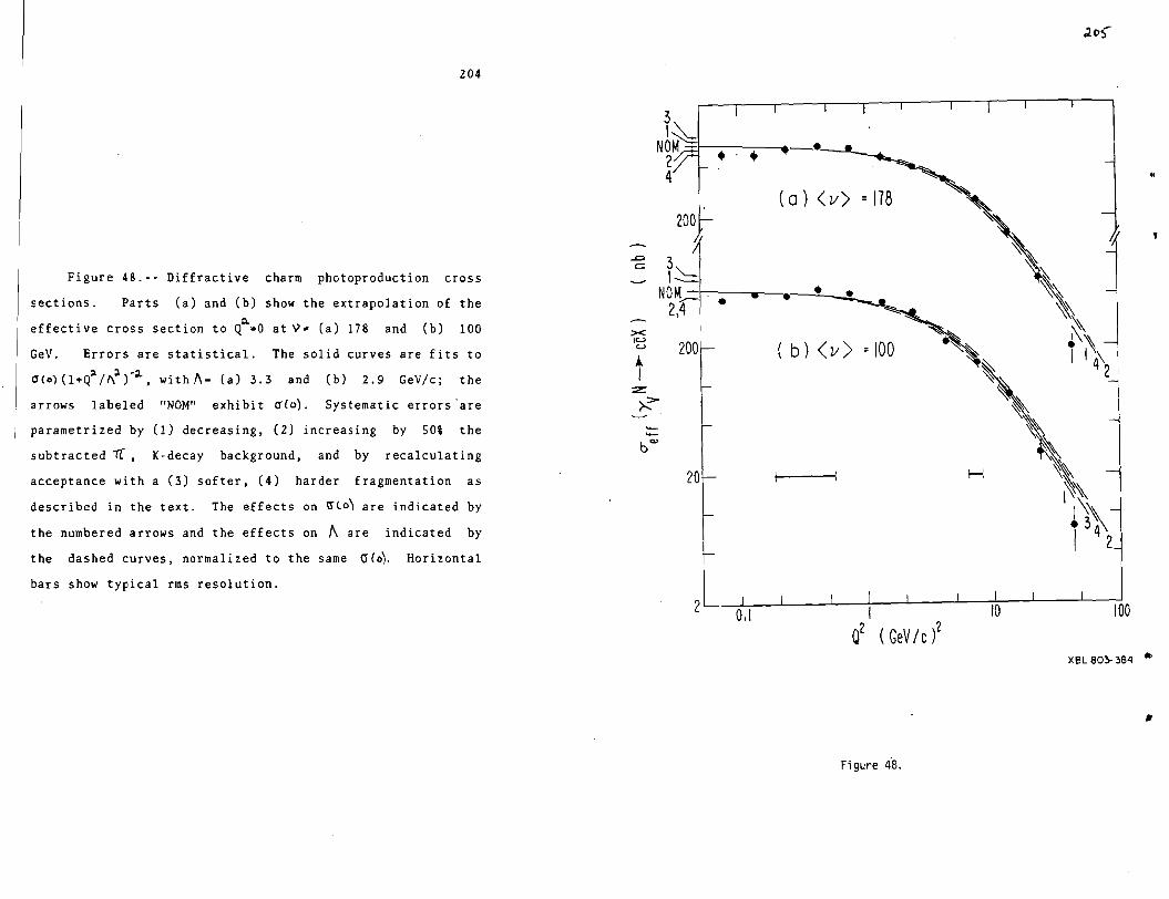
204
Figure 48.-- Diffractive charm photoproduction cross
sections. Parts (a) and (b) show the extrapolation of the
effective cross section to Q::>..=0 at 'V= (a) 178 and (b) 100
GeV. Errors are statistical. The solid curves are fits to
OCo) (l+Q-;a./l\l)-:J.., with.f\= (a) 3.3 and (b) 2.9 GeV/c; the
arrows labeled "NOM'' exhibit alo). Systematic errors 'are
parametrized by (1) decreasing, (2) increasing by 50\ the
subtracted T[ , K-decay background, and by recalculating
acceptance with a (3) softer, (4) harder fragmentation as
described in the text. The effects on ~to) are indicated by
the numbered arrows and the effects on A are indicated by
the dashed curves, normalized to the same 0(~. Horizontal
bars show typical rms resolution.
r~ NOr 2/:r • • • 4
200
~
3"-c , __ NO!{,::
2,4 • >< I"-' 200 u
t = ~ ._ ._
b Q.)
20
-·~ "'!!!, ..
(a) < v) = 178
~~
·\\ • • \\ ~~
~ ( b) < v > = 100 . :\
~ I I 4\2 I
~~ 1 ~~ ~~
H ~ ~\
t\\
XBL80~~84 •
Figure 4·8.

206
Figure 49.-- The role of charm in the rise of the ~N
total cross section. Data points representing the effective
photon cross section (right scale) are compared with a fit
from Ref. 64 to half the photon-deuteron cross section
(curve, left scale). Systematic uncertainties dominate the
errors.
c:> ~
t l.J...J __J
<.:C <...-> c:> U) ~ =
>-Q.> ~
...__...
>-.. l.J...J
r<"l co r<"l ' r<"l
0 CD ...J CD x
~ .,;-
QJ ... ~
C'>
LL

208
Figure 50.-- Energy-dependence of the effective cross
section for diffractive charm photoproduction. For :t '- ~
0.32<Q <l.B(GeV/c) , crcff varies with Q by ~ 20%. Errors
are statistical. The solid curve exhibits the v-dependence
of the photon-gluon-fusion model with the "counting-rule" S'
gluon ~ distribution 3(1-~) /~, and represents the data
with 13% confidence. Other gluon-distribution choices
(1-Xg)q/xj, and "broad glue" (1-x~/(13.5+1.07/x3 ) (Ref. 17)
are indicated by dashed curves. The dashed curve labeled BN
is the phenomenological parametrization of Ref. 66, and the
dashed horizontal line represents energy-independence.
Curves are normalized to the data. The shaded band exhibits
the range of changes in shape allowed by systematic
uncertainies. For visual clarity it is drawn relative to
the solid curve. Data below V =75 GeV are excluded from
further analysis.
0.8
-= :::i_ - 0.6
>< le..>
<:..>
t ::z::
>-
>---4-- 0.4 4--
Q;>
b
0.2
50 70 100 140
v (GeV)
Figure 50.
(\-X)9/x .,,, .. ,,,,,,,,,.,,."· B N
;"'·''/:;>/}\);;""8 U -x) 5 Ix
"BROAD GLUE"
280
XBL 803-366
I~

..
•
210
~ Figure 51.-- Q dependence of the structure function
F~(cc) for diffractive charm muoproduction. At each of the
two average photon energies, each curve is normalized to the
data. Errors are statistical. The solid (short dashed)
curves labeled mc=l.5 (1.2) exhibit the photon-gluon-fusion
model prediction
GeV/c~. Solid
with
curves
a charmed quark mass of 1.5 (1.2)
labeled 'f nM correspond to a
'f-dominance propagator, and long-dashed curves labeled BN
represent the model of Ref. 66. Shown at the top is a fit
adapted from Ref. 20 to the inclusive structure function F~
for isospin-0 muon-nucleon scattering. The shape variations
allowed by systematic errors are represented by the shaded
bands.
0.5
>< :::l
t = :::l
"' ...... 0.1
~ 0.001
:::l
t = :::l
0.0002 '-----0...L. l----'---'---'--I _ _,__ _ _,__l"--0 _ _,___~~100
rJ ( GeV Id
Figure 51. XBLS03- 38Z
.;LI I

212
Figure 52.-- Scale-noninvariance of F1 (cc). Data
points are arranged in pairs, alternately closed and open.
The points in each pair are connected by a solid band and
labeled by their common average value of Bjerken x =
Q;i./( 2Mv). Errors are statistical. The dashed lines are
predictions of the photon-gluon-fusion model with mc:.:i.s
GeV/c;i. except that the model is renormalized and damped at
high Q~ as described in the text. The solid bands represent
the slope variations allowed by systematic errors. The
dot-dashed lines represent the changes in Fi(cc) as Q;i. is
increased but x is held constant that would be necessary to
equal the changes in the CHIO fit to F~ which occur under
the same circumstances. The percentages next to these lines
indicate the relative sizes of the changes in F1 (cc) and F~,
fit by CHIO.
~ 0
ID - --
~ .., ---8 ci
6 ci
8 0 ci
(X~'Jr/-Nrf)
/ I
~I 0\
\
N 0 0 ci
' ' ' ,,........_
6 Cl 0
.. ,
,,
-Q
N - N u II>
:> QJ ,_ Cl) "' (.!) Cl
·~ u.
N 0


