
Linking staples-led growth, economic development and the distribution of wealth: Evidence from a natural experiment comparing Canada and
South Australia
by
L. Di Matteo1, J.C.H. Emery2 and M.P. Shanahan3*
1 Department of Economics, Lakehead University, Thunder Bay, Ontario, Canada 2 Department of Economics, University of Calgary, Calgary, Alberta, Canada
3 School of Commerce, University of South Australia, Adelaide, Australia
[VERSION OF MAY 6, 2008]
DRAFT: NOT FOR QUOTATION
* Livio Di Matteo acknowledges the support of the Social Sciences and Humanities Research Council of Canada. Herb Emery acknowledges the support from the School of Commerce, University of South Australia that allowed him to visit and which resulted in this collaboration. Martin Shanahan acknowledges the assistance of an Australian Research Council Grant in supporting this research and thanks John Wilson for research assistance. The authors thank participants at the Canadian Network for Economic History Conference at Kingston, Ontario, for their comments.

2
ABSTRACT
The literature on the linkages between national development, factor endowments, and institutions views inequality as one factor contributing to institutional quality. Examining these links, such research regularly groups ‘like’ countries such as Canada and Australia in contrast to underdeveloped countries. Similar over-simplifications occurred in the discussions on staples-led development in the 1960s. This paper takes advantage of a natural experiment by comparing two ‘like’ regions, the Thunder Bay District in Northwestern Ontario and the state of South Australia between 1905 and 1915 to highlight their similarities and differences. These two regions, both large wheat exporters with similar institutional heritage, represented very different parts of the export chain. By comparing the level and composition of wealth and wealth inequality found in each region we conclude that long term economic development from natural resources may well be a function of the ability to retain linkages. However, whether an economy diversifies or remains staple dependent is the outcome of a delicate balance between the level, compositon and distribution of the wealth generated.

3
INTRODUCTION In his 1989 Tawney Memorial Lecture, C.B.Shedvin concluded
The optimistic version of the staple thesis suggests that the linkage effects
of staple production will generate significant structural change and a break
from previous path dependency. This mirrors Canadian experience but it
seems that Canada may be exceptional and that the break from staple-
induced path dependency is usually difficult to achieve…1
In explaining how and why Canada’s growth experience had followed the ‘optimistic
liberal version of steady progress from staple production to a broadly based industrial
society’2 Schedvin contrasted the experience of Australia which he argued had fallen into
the ‘staple trap’. There the ‘tendency has been to move from one dominant staple to
another, but there has been little export diversification… The dominant staples have
generated high income levels, but in the long run relative incomes have declined because
of adverse movements in the terms of trade and the inability to move into high value-
added production’.3
We compare accumulated personal wealth stocks in the Thunder Bay District
(TBD), Ontario, Canada and in South Australia (SA) to examine one previously
neglected ‘marker’ behind successful and unsuccessful development from natural
resource exports. We look at the effects of a common resource for export, wheat, in the
same decade, 1905 to 1915, in these two British settler economies.
The first section of this paper discusses aspects of the staples led model of
economic development, and highlights the similarities with the pessimistic view of this
form of development and the ‘resource curse’ literature. The second outlines the
similarities and differences between the TBD and SA in the decades prior to World War
I. Third, we detail our data while in the fourth section we compare wealth levels and
trends in each region between 1905 and 1915. The results suggest that South Australia
represents an economy where transportation, production and handling of wheat are
carried out by local owners of capital so that capital’s share of income is retained locally.
1 Schedvin, “Staples and Regions” p557. 2 Schedvin, “Staples and Regions” p534. 3 Schedvin, “Staples and Regions” p536.
4
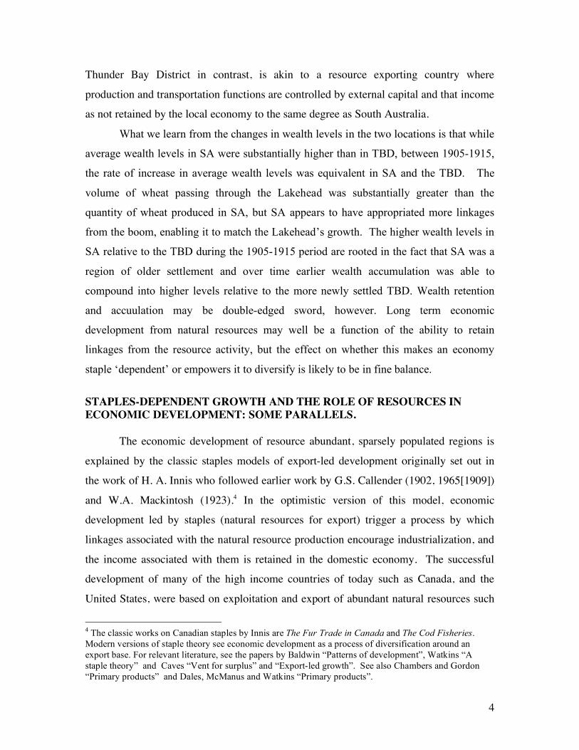
Thunder Bay District in contrast, is akin to a resource exporting country where
production and transportation functions are controlled by external capital and that income
as not retained by the local economy to the same degree as South Australia.
What we learn from the changes in wealth levels in the two locations is that while
average wealth levels in SA were substantially higher than in TBD, between 1905-1915,
the rate of increase in average wealth levels was equivalent in SA and the TBD. The
volume of wheat passing through the Lakehead was substantially greater than the
quantity of wheat produced in SA, but SA appears to have appropriated more linkages
from the boom, enabling it to match the Lakehead’s growth. The higher wealth levels in
SA relative to the TBD during the 1905-1915 period are rooted in the fact that SA was a
region of older settlement and over time earlier wealth accumulation was able to
compound into higher levels relative to the more newly settled TBD. Wealth retention
and accuulation may be double-edged sword, however. Long term economic
development from natural resources may well be a function of the ability to retain
linkages from the resource activity, but the effect on whether this makes an economy
staple ‘dependent’ or empowers it to diversify is likely to be in fine balance.
STAPLES-DEPENDENT GROWTH AND THE ROLE OF RESOURCES IN ECONOMIC DEVELOPMENT: SOME PARALLELS.
The economic development of resource abundant, sparsely populated regions is
explained by the classic staples models of export-led development originally set out in
the work of H. A. Innis who followed earlier work by G.S. Callender (1902, 1965[1909])
and W.A. Mackintosh (1923).4 In the optimistic version of this model, economic
development led by staples (natural resources for export) trigger a process by which
linkages associated with the natural resource production encourage industrialization, and
the income associated with them is retained in the domestic economy. The successful
development of many of the high income countries of today such as Canada, and the
United States, were based on exploitation and export of abundant natural resources such
4 The classic works on Canadian staples by Innis are The Fur Trade in Canada and The Cod Fisheries. Modern versions of staple theory see economic development as a process of diversification around an export base. For relevant literature, see the papers by Baldwin “Patterns of development”, Watkins “A staple theory” and Caves “Vent for surplus” and “Export-led growth”. See also Chambers and Gordon “Primary products” and Dales, McManus and Watkins “Primary products”.

5
as fish, fur, timber, gold, grain, coal and oil.5 The pessimistic version of this model,
however, highlights the view that staple-led development can lead to a ‘trap’ whereby the
economy is overly-dependent on external markets, distorted and subject to instability
flowing from variations in staple prices.6 While Argentina and the ‘old south’ of the USA
are cited as classic exemplars, writers such as McCarty and Schedvin have highlighted
Australia’s and New Zealand’s similar, but less extreme, progress along this path.7
In a debate that resonates with the pessimistic view of staples-led development,
Sachs and Warner show that resource abundant economies (as measured by export
dependence on natural resources) have had slower growth than resource scarce
economies since 1970.8 This negative correlation between natural resource exports and
growth has been dubbed the “resource curse” and has triggered a sizeable literature that
seeks to explain this surprising outcome. As Sachs and Warner note, the resource curse
is a surprising phenomenon given the expectation that resources are a catalyst for
development.9
Unfortunately, Sachs and Warner dismiss the relevance of historically successful
resource based development cases for understanding the resource curse.10 First, they
argue that these successful countries developed in a world of relatively high
transportation costs that encouraged manufacturing and processing industries to locate
near available resource endowments such as coal and that they never had as intensive
exploitation of natural resources compared to resource dependent economies of the mid-
to late 20th century.
5 The staples approach with its focus on natural resource exports has served as an explanatory framework for nineteenth century Canadian and Australian economic history. A comparative study of the success of staples in Canada, Australia and Argentina is provided in Fogarty “Economic history”. For a comparison of Canada and Australia, see Pomfret “The staple theory”. For the role of natural resources in U.S. development, see Wright and Czelusta, “Why economies slow”. For other perspectives on export-led growth see Anderson “Regional trade and adjustment” and Regional Economic Analysis, Harley “Resources and economic development”, Corden “The economic effects” and Corden and Neary “Booming sector and de-industrialization”. For other accounts on the Canadian wheat boom, see Bertram “The relevance of the wheat boom”, Lewis “The Canadian wheat boom”, Harley “Western Settlement and the Price” and Fowke The National Policy. 6 The taxonomy is from Schedvin “Staples and Regions” pp 533-535. 7 McCarty , “The staple approach”. 8 Sachs and Warner, “Natural resource abundance”; and “The big Push” The parallel between staples theory and raw material-based growth was articulated by North “Location theory”. 9 Sachs and Warner, “Natural Resources and Economic Development” 10 Sachs and Warner, “Natural resource abundance”

6
This view neglects that in the absence of protectionist policies, countries like Canada and
the United States primarily exported raw, or unprocessed, natural resources and imported
much of the manufacturing needs from the distant British market. Crafts notes “that the
United States was a high tariff country throughout its rise to world economic
leadership”.11 If the abundance of local power sources and resources for inputs into
manufacturing were the key determinant of industrialization, then the failure of much of
the US northeast, and Northern Ontario in Canada, to industrialize and develop stand as
important historic counter examples. If we consider the resource intensity of Canada and
the United States just prior to their creation as nation states, then we see their successful
development began as resource based economies.12 Further, Auty argues that there is
nothing deterministic about resource abundance and successful development and
sustained growth.13 He notes that many resource abundant economies grew rapidly
between 1870-1913 and 1950-1973. The growth collapses of the late 1970s and early
1980s of resource dependent economies is ironic, he says, since the collapse was the
result of resource dependent economies trying to reduce their resource dependence.
Counter to the view of Sachs and Warner, the explanation for the “resource
curse” may indeed be found in an understanding of why successful natural resource based
development has occurred historically but not recently. In particular, an historical
perspective allows a closer examination of one particular aspect of the process by which
staples, or natural resources, effect development; income (and subsequent wealth)
11 Crafts, “Globalisation and Economic Growth” p .54. 12 Hughes and Cain, American Economic History, p. 30, show that in the Colonial economy of the 1700s, nine-tenths of the population were employed in agriculture, fishing, timbering and mining. McCallum Unequal Beginnings shows that in the mid-nineteenth century Ontario, Canada’s industrial heartland today, two-thirds of its population were engaged in farming with substantial cash sales generated from wheat production and 80 percent of wheat production exported. A comparison of export to GDP ratios for nation states can be mis-leading at any point in history, and particularly mis-leading when comparing across time. Comparing countries of large area like the United States, Canada or Australia, where there are several identifiable regional economies engaged in inter-regional, as well as international, trade with smaller area, single region nations like Kuwait is misleading. While the Canadian and United States national economies may not be as resource intensive as some of the resource abundant economies of today, some sub-national economies were and are intensive exporters of natural resources. For example, for the Provinces of Alberta and Saskatchewan, natural resource (international) exports in 1984 were 35 percent of provincial GDP which is higher than Nigeria, Venezuela and Iran in 1970 as shown in Sachs and Warner’s “Natural Resources and Economic Development” Figure 1. 13 Auty, “The Political Economy of Resource-Driven Growth”

7
distribution.14 The work of Baldwin is particularly apposite here.15 He argued that the
distribution of income directly effected demand linkages on the one hand, and
productivity, and hence the supply side, on the other. On the demand side, he suggests,
unequal income distribution results in the disproportionate importation of luxuries and
the underdevelopment of local industries to supply the demands of high income earners.
Further, conspicuous consumption results in lower investment-savings. On the supply
side, low incomes to workers reduces labour productivity, which over time reduces
relative efficiency and pressure for technological change. Where income is unequally
distributed, he suggests, the benefits of staples led development are hampered.
Probate records, which can reveal the accumulated wealth of individuals collected
over their life-time, should provide some evidence of the extent to which income
generated from staples-led exports was captured and distributed. It should also allow
insight into whether variation in the types of assets held by individuals was consistent
with Baldwin’s hypothesis. If probate records reveal high quantities of luxuries and
personal assets among probated estates in regions with subsequent slower economic
diversification there is at least circumstantial support for the argument that wealth (and
by inference income) distribution matters. To this end, we examine the level, distribution
and composition of wealth of probated decedents in the Thunder Bay District, Ontario,
and in South Australia over the period 1905 to 1915. We are interested in examining
how much wealth accumulated during wheat export booms; how much of that wealth was
invested in the local economy, and how much was held in assets external to the local
economy. Wealth is in many ways a superior variable to income for our purposes,
because it can capture the long-term impacts of the effect of natural resource exports on
economic development.16 The asset composition of that wealth can also reveal something
about the type of long-term consumption enjoyed by wealth leavers. We thus interpret the
14 The standard works are Chambers and Gordon “Primary products and economic growth” and Caves, “Vent for surplus” and “Export-led growth.” For a summary see Altman “Staple theory and export led growth” 15 Baldwin “Patterns of development” 16 Chambers and Gordon “Primary products and economic growth” show that the effect of natural resource exports on long run per capita income growth will reflect the increase in the value of “land”, the fixed factor in natural resource exploitation. See Hartwick “Investment of rents” and Rodriguez and Sachs “Why do resource abundant economies grow” for the reasons why resource exporting economies need to save and invest resource rents in order to sustain consumption levels experienced during the resource boom.

8
accumulation of wealth in a resource-based economy as a marker of the nature of its
staple-led development.
SOUTH AUSTRALIA AND THE THUNDER BAY DISTRICT: A BRIEF
COMPARISON AND HISTORY
Despite geographical and social differences, institutional quality in the
communities of South Australia and the Thunder Bay District should be comparable.
Both were regions with representative government, well-established property rights and
comparable (if different) English legacies in their social attitudes. In the first decades of
the 20th century both were in transition from being under-developed regions on the
periphery of the world economy to regions where the communities aspired to achieve
some of the material outcomes and comforts found in the more developed core.17
There are also differences between the two regions that may be informative for
identifying the ways in which natural resource exports influence economic development.
While both regions benefited from the extension of the agricultural frontier and biological
and technological innovations in wheat production,18 South Australia’s benefits were
encompassed by her borders. Thunder Bay benefited more indirectly from such
innovations as it mostly served as a transshipment point without the direct benefit of
regional wheat production.19 Also, South Australia benefited from earlier resource export
episodes, including copper in the 1840s, wheat and wool in the 1850s and wheat again in
the 1870s. On the other hand, the Thunder Bay District and its port towns of Port Arthur
and Fort William (collectively known as The Lakehead) was really a new economy in
1905. By 1905, South Australian exports, despite still traveling longer distances to their
markets than those from Thunder Bay, had been attuned to the demands of external
buyers for 50 years.
17 Harley 2007 18 For a discussion of biological and technological innovation in wheat production, see Olmstead and Rhodes “The Red queen and the Hard Reds”. 19 Gallup, Sachs and Mellinger “Geography and Economic Development.” and Rappaport and Sachs “The United States as a Coastal Nation” also highlight the positive correlation between coastal locations and income levels but do not satisfactorily explain why the correlation exists. The grain production in the SA economy was for the most part contained within 60 miles of coast, and all within its state borders, whereas Port Arthur/Fort William was an intermediate terminus on the Canadian transportation system; grain being transferred from Great Lakes Freighters to ocean going vessels on the way to market.

9
The years 1905 to 1913 were an important period for the economic development
of both the Thunder Bay District and the South Australian economy even though they
were at different stages of development. For the TBD, this was the period of substantial
initial development while for the already established SA, the period saw the return of
prosperous economic conditions following more than a decade of economic stagnation.
While European settlement of the Thunder Bay District began during the fur trade
when it was home to Fort William, the inland headquarters of the Northwest Company of
Montreal, it was the coming of the transcontinental railway in the 1880s that linked the
region to the Prairie wheat economy and central Canada and spurred the region’s
development. The Thunder Bay District was uniquely juxtaposed between the Prairie
wheat economy, from which it would benefit by having its major metropolitan centre
serve as entrepot, and central Canada, where it was part of Canada’s wealthiest province.
The northwestern portion of the province, along with the Thunder Bay District, was
directly tied to the Prairie wheat boom via the grain port function of the twin cities of
Fort William and Port Arthur known collectively as the “Lakehead”.20 Moreover, a
portion of the economy was rooted in local manufacturing development, resource
extraction and agricultural development.21
The population of the district grew rapidly with the greatest expansion between
1901 and 1911 when the population nearly tripled to approximately 40,000. Most of the
population growth during the boom period occurred at the Lakehead as the result of high
in-migration and by 1921 over 70 percent of the District’s population was at the
Lakehead. The economic boom at the Lakehead ended with the onset of the First World
War. The increase in interest rates in 1913 tightened farm credit and halted the expansion
of the wheat boom that was then followed by the disruption of the war and the reduction
in immigrant flows to the west. The opening of the Panama Canal in 1914 may have also
redirected some of the flow of wheat and commerce away from the Lakehead and to the
west coast. The value of building permits in Fort William rose steadily from 1907 and
peaked in 1912 at just over 4 million dollars and then fell dramatically for the next four
20 Di Matteo, “Economic development of the Lakehead”, “Evidence on Lakehead”, “Booming sector”. 21 Gross regional product in the absence of the wheat boom at the Lakehead would have been 42 per cent smaller. In addition, by 1921, there were 1,534 farms supporting a rural population of 7,397 around the Lakehead. Forestry also employed thousands, in extraction, at sawmills and at the three pulps mills either operating or under construction by 1921. See Di Matteo, “Booming sector”, pp. 611-614.

10
years to reach 0.6 million dollars by 1916. At least a dozen major employers shut down
from 1914-22 and the size of the labour force declined. Recovery did not begin until the
construction of the first pulp mill in 1917.22
The European settlement of South Australia was just over 70 years old in 1905.
South Australia had a rural-based economy founded under a system of ‘systematic
colonization’ to produce a self-supporting system financed by land sales. Despite initial
difficulties, within twenty years of settlement the colony boasted a population of 85,000
and over 160,000 acres of wheat were sown, with a large portion being used to feed the
gold rushes in the neighboring colony of Victoria.23 Indeed so successful was South
Australia in agricultural pursuits that by the 1870s it was regarded as ‘the granary of the
continent’.24 By 1901, the first year of Australian federation the population of the new
state of South Australia was 359,000, with 162,000 or just over 42 percent living in the
capital Adelaide.25 A decade later the state’s population reached almost 410,000, with
Adelaide accounting for around 50 percent of the population.26
SA was geographically distant from the Atlantic economy, but culturally and
historically linked to England. Although distant from the centre of world financial
markets in London and the newly emerging industrial strength of North America, it still
felt itself to be part of the modern industrial world. Changes in transportation affected
the State’s external trade. The great circle route (south from England until the roaring 40s
below South Africa, west to Australia and then after leaving Australia, back to 40o south
and around the Cape of Good Hope) meant that in the 1870s clippers took 80 days to get
to England. The opening of the Suez Canal in 1869 and the rise of steamships changed
the technology of shipping, although by 1883 still only one-third of cargo returned to the
22 Stafford, “Century of growth”, pp.44-45 and Di Matteo, “Evidence on Lakehead”. 23 Stevenson, “Population Statistics” Tables 1.1 p13. 24 Shaw, The story of Australia, p.168. 25 Hirst, Adelaide and the Country, pp 227-228. 26 In 1911 the population of Adelaide was just under 190,000, representing 46.4% of South Australia’s population. Equivalent figures for 1871, 1881, 1891 and 1901 are 33.8%, 37.6%, 42.2% and 45.3%. By 1921 the percentage was 51.6 % (Hirst, Adelaide and the Country, pp 227). Ontario had a more dispersed urban settlement pattern. In 1891, Toronto - Ontario's largest city - had a population of 181,000 which represented less than 10 percent of the province's population. In 1891, only 35 percent of Ontario's population could be considered urban - that is living in centers of 1000 or more.
11
UK via the Suez. It was not until 1911 that steamers replaced clippers in the wheat
trade.27
Despite South Australia’s early expansion in wheat exports (and lead in the use
of agricultural machinery), it took some time for farmers to understand their environment.
From the mid 1850s average yields declined in South Australia until a slight upturn in the
late 1860s. Offsetting the decline was the expansion of acreage. It was not until new
varieties of wheat were developed and planted in the late 1890s, and these were
combined with more effective use of fallowing and fertilizers that average yields per acre
again increased.28
A major factor impacting on the South Australian economy was drought.
Droughts of differing levels of severity occurred in the 1860s and the 1880s, while the
combination of the depression in the early 1890s followed by one of the worst droughts
ever recorded (from 1895-1903) put significant brakes on economic prosperity. A further
drought at the end of World War I slowed economic recovery.29 The First World War
not only made trading agricultural products with Europe difficult, it also impacted
heavily on the workforce. The period from 1914 to the 1940 was one of relative
stagnation of living standards for the whole of Australia, and South Australia was not an
exception.30
Apart from remaining preeminent in wheat production within Australia until the
1890s, South Australia also developed a significant pastoral industry. Together these
gave the economy a large agricultural base for wealth accumulation, as well as heavy
exposure to drought risk. While no extensive gold deposits were found in South
Australia, copper deposits north of the capital provided an alternative resource export for
over 60 years. Wheat, wool and copper, together with benefits of being the nearest capital
27 According to Dunsdorfs The Australian wheat-growing industry (footnote 12, page 172) “Steamships became firmly established in the wheat carrying trade only between 1905 and 1909, or even 1911. The Official Yearbook for New South Wales reported for the year 1905-06 (p.349) that three-fourths of the wheat exported was carried by sailing vessels. For 1911 the same source (p 438) states that since 1909 sailing vessels had been replaced by steamers: “…the proportion of wheat now carried in sailing vessels is very small”.” 28 In this SA has remarkable similarities with wheat expansion in the United States and Canada. Olmstead and Rhodes “The Red queen and the Hard Reds”. 29 For example, in pre-drought 1891 there were 7.6 million sheep in South Australia; by the end of 1914 there were only 3.6 million. (Vamplew South Australian Historical Statistics, Table 11.9) 30 McLean and Pincus, “Did Australian living standards stagnate”

12
to the silver and lead deposits at Broken Hill underpinned Adelaide and South Australia’s
growth through the 19th century. Compared to the other states of Australia, South
Australia had the advantage of agricultural land that was comparatively close to the
capital, and relatively easy to clear.31 This also contributed to development of a network
of rail lines, many of which initially carried wheat to Port Adelaide and from there,
directly to London.32 From the 1870’s many rail lines linked inland farmers directly to
ports outside of Adelaide.33
The onset of Australian Federation in 1901 also brought a change to trade
arrangements. As a colony, South Australia had levied its own tariffs and customs prior
to 1900. Until 1877 there was a 10 per cent ad valorem duty on imported wheat while
from 1888 until 1900 South Australia charged 2 shillings per cental (100 pounds) on
wheat. Only Victoria was seen as being seriously protectionist in outlook and practice.34
Federation removed customs duties between the states, while overall Australia, like
Canada, adopted a protectionist regime.35 Thus, prior to 1900, SA had the unique ability
to capture linkages through protectionist policies, but after 1900, they were not able to do
this. On the other hand, the TBD was never able to set its own independent tariff policy.
South Australia benefited not only from the transport of grain via Adelaide but
also from the actual production of wheat in the region. In other words, it also earned
rents from the land factor which would not have been available in the case of Thunder
Bay. The Thunder Bay District benefited from transporting prairie grain in a manner
described by McCallum – the appropriation of linkages from a staple produced far from
the region.36
31 Dunsdorfs The Australian wheat-growing industry, pp 99-106. 32 Until the 1870s Australia as a whole was not a consistent exporter of wheat with the colonies of New South Wales, Victoria and Queensland being net importers until 1867. Against this trend South Australia became a net exporter comparatively early, exporting a (then record) 3 million bushels to Great Britain in 1872. Despite large annual fluctuations (that impacted on the local economy) this trade continued through the period of interest (Dunsdorfs, The Australian wheat-growing industry, pp167-168). Note too that in 1870 there were only 133 miles of railway open in South Australia, while by 1900 there were 1,736 miles- two thirds of this being built after 1880: Butlin, Investment in Australian p.321. 33 Meinig, On the margins, pp 124-165. 34 This section leans on Dunsdorfs, The Australian wheat-growing industry, p 165-167. 35 Pomfret, “Trade policy in Canada and Australia”, p 116. In 1913 Canada had an average tariff of 18% and Australia 17%. 36 McCallum Unequal Beginnings

13
While the Lakehead towns were the dominant metropolis of their region, their
economic growth was largely dependent on their transshipment function which they
increasingly had to share with Vancouver, Montreal and Quebec City; they did not have
access to the equivalent of Adelaide’s compact agricultural hinterland. The railways that
shipped grain to the Lakehead and the shipping companies that took the grain from the
Lakehead represent external capital/businesses for the Thunder Bay district and as such,
the share of income earned by that capital was less likely to have been retained in the
region. Adelaide residents, however were likely to have possessed a greater locational
monopoly on grain shipping out of their relatively compact region. Despite the
development of ports along the coast in the 1870s, the rail network consisted of “long
extensions deep into the interior, not only to serve the pastoral and mining regions, but
also as instruments of grand strategy to capture a major share of the interior trade of
neighboring colonies.”37 Moreover, all railways in SA were state owned so that the
transportation income was retained in the SA economy.
South Australia had a substantial head start in terms of economic development.
While 1885 represents the dawn of grain shipping at the Lakehead and the full prairie
wheat boom was still over a decade away, in 1885, South Australia exported almost 8
millions bushels of wheat and flour and the population of South Australia was over
70,000.38 However, during the period 1905-1915, when wheat production boomed in
Canada and regained ground after years of drought in SA, the volume of wheat
production in Canada far exceeded that of South Australia and indeed the volume of
wheat shipped through the Lakehead was far greater than that through Adelaide. Whereas
South Australia’s wheat production and exports during the 1880s were comparable in
scale to those of the Ontario economy in the 1850s and 1870s,39 the 1905 to 1915 period
37 Meinig On the margins p.140. As a further example of the possibilities to ‘extract more’ from wheat production, The 1908 Royal Commission on “The Question of the Marketing of Wheat” in South Australia, found that merchants purchasing wheat from farmers colluded so as to reduce the prices received by farmers by 1d to 2d per bushel. A similar enquiry in Victoria found evidence of ‘sharp practice’ that resulted in wheat bags being systematically under-weighed by 1.1 to 3.3 per cent. (Dunsdorf, The Australian wheat-growing industry pp 223-226). 38 Canada exported 5.2 million bushels of wheat and flour in 1885 (Leacy, Historical Statistics of Canada, Series M305). By 1911, exports of wheat and flour from Canada reached 98 million bushels. 39 See McCallum Unequal Beginnings, Table s.3 .
14
saw wheat shipments through the Lakehead that dwarfed the size of wheat production
and exports of SA (See Table 1).
Nonetheless, in relative terms, wheat was extraordinarily important to South
Australia for many years. Between 1860 and the mid 1890s, between 60 and 80 percent
of South Australia’s wheat production was exported, mostly to the UK.40 In South
Australia in 1870, the agricultural (12.6%), pastoral (14.48%), and dairy sectors (3.15%)
contributed one-third of the colony’s GDP and by 1910, this had fallen slightly to 29
percent with agriculture (mostly wheat) contributing 17 percentage points.41 In
comparison, Canada in 1870, agriculture’s (all kinds) share of GDP was 28 percent and
by 1910, it was a little over 20 percent. For Canada in 1870 wheat contributed 4.5
percent to GNP (0.16 of 28%), and by 1910, 4.8 percent (0.24 of 20%).42 Despite South
Australia having been overtaken at the end of the 19th century as the single largest wheat
producer in Australia by Victoria and New South Wales, we estimate that wheat’s
contribution to state product had fallen to ‘only’ 6.97 percent of South Australia’s gross
state product (0.41 of 17%).43
THE DATA
Given both countries sold on the world wheat market between 1905 and 1915, the
Canadian grain economy should have generated income at the Lakehead many times
larger than that seen in SA. There are two ways in which these differences could be
apparent; in the overall increase of the economy and population, and to the extent that
linkages are retained/captured; in wealth estimates. Wealth is a better measure for
evaluating the long term impacts of natural resource exports than current income,44 thus
we focus on estimates on the distribution and composition of personal wealth, and
40 Dunsdorfs The Australian wheat-growing industry, p 168. 41 Sinclair The process of economic development. 42 Urquhart Gross National Product. 43 This last figure may under-estimate wheat’s importance to the SA economy. It is calculated by using Butlin’s national figures on the contribution of wheat to agricultural output in 1910/11 (41% by value) (Butlin, Investment in Australian, Table 44 p 96). 44Hartwick “Investment of rents” and Rodriguez and Sachs “Why do resource abundant economies grow”. Chambers and Gordon “Primary products and economic growth” show that the effect of natural resource exports on long run per capita income growth will reflect the increase in the value of “land”, the fixed factor in natural resource exploitation. In other words, the value of rents should be reflected in real estate values.

15
average wealth levels over the period as an indicator of the effect of natural resource
exports on development. We are interested in examining how much wealth accumulated
during these wheat export booms; how much of that wealth was invested in the local
economy, and how much was held in assets external to the local economy.
The South Australian data are derived from probate and succession duty
documents which are constructed after the death of an individual. Essential to the legal
transfer of assets, these represent consistent, well-monitored information on personal
wealth. Probate records contain papers filed to the court by the administrators of an
estate including a copy of the testator’s will, the executor’s oath, correspondence with the
court etc.. The records contain information on the testator’s name, address, occupation
and a sworn estimate of gross wealth; but no list of assets, the age of the testator, and
other family details. To obtain this information it was necessary to match the probate
records with two other sources; the individual’s death certificate and succession duty
records. The death certificate contained information on the testator’s age and cause of
death as well as providing a cross check for recorded occupation. Between 1905 and
1915 the state levied succession duty on all estates and this process produced a
succession file which contained a full inventory of the assets of the deceased, their heirs
and the duty payable on each inheritance. The succession duty process required an
independent appraiser estimate the market value of each individual piece of property,
which may include assets as trivial as salt and pepper shakers or as large as pastoral
stations or manufacturing businesses.45
The Ontario data set was constructed from the probate records of the District of
Thunder Bay Surrogate Courts from years 1885 to 1920. Prior to the Thunder Bay
District's creation in 1885, the region’s estates were probated in the District of Algoma.
Under the Surrogate Courts Act, 1858 (Statutes of Canada, 22 Vict., Cap. 93, 1858) a
surrogate court with the power to issue grants of probate and administration valid
throughout the province was established in each Ontario County, replacing the
centralized Court of Probate established in 1793. The inventory was conducted by the 45 For the purposes of constructing a data set from the probate data, four strata were selected. A one percent sample of estates between £0 and £500; a two percent sample for estates between £501 and £2500; a five percent sample of estates between £2501 and £20,000 and the complete population over £20,000. Records of a total of 337 individual estates were recorded but exact date of probate was only available for 307 of which two had negative net wealth leaving 305.

16
executor of the estate (administrator in intestate cases) and legally needed only to be
performed in response to a request by a legatee or creditor but in practice was brought in
voluntarily without awaiting the compulsory summons.46
All estates bearing application dates in the years 1885 to 1920 were examined but
only those 591 estates from 1905 to 1915 are used in this paper for comparison purposes.
Variables recorded include place of residence, occupation, marital status, number of
children, date of death, whether they had a will and the value of the estates.
Unfortunately, age at death was not available in these probate records.47 The inventory
provided estimates of wealth grouped into 16 categories.48 Like the Australian data an
advantage of this data source is that there are separate estimates of real estate, financial
assets and personal property over a substantial period of time.
One of the potential differences between the two data sets is the presence of age
differences between a region that had a longer established pattern of settlement and one
currently undergoing a settlement boom. While age data are not available for the set of
Thunder Bay probated decedents, Thunder Bay is part of northern Ontario and census-
linked data constructed for Ontario for 1892 and 1902 reveal the average age of northern
Ontario residents in 1892 was 50.7 years and in 1902 was 50.8. The average age for the
South Australian decedents was older at 63.4 years, which corresponds to the average age
of all Ontarians in the 1892 and 1902 data (61.2 and 61.7 years respectively). This
46 According to Howell’s Law and practice, pp. 325-326: “The inventory should contain a statement of all the goods, chattels, wares and merchandize, as well moveable as not moveable, which were of the person deceased at the time of his death within the jurisdiction of the court. A proper inventory should enumerate every item of which the personal estate consisted, and should specify the value of each particular. But unless by order of court, or in obedience to a citation, an inventory does not set forth the goods and chattels in detail.” Probate instructions do not specify how asset value was assigned. For real estate, livestock and personal property the evidence suggests that it was market value. Sometimes, property was sold and its selling price recorded in the inventory, whereas more often it was an estimate of what the property would fetch if sold. Financial assets by their nature were precisely recorded. Mortgages held, the amount of insurance payments, and bank account balances were precise amounts. In addition, real estate was usually recorded net of any mortgages outstanding. 47 Some data on age could be acquired by census-linkage but only three census years (1881, 1891, 1901) are currently available. 48 The inventory categories were: (1) Household goods and furniture, (2) Farm implements, (3) Stock in trade, (4) Horses, (5) Cattle, (6) Sheep and Swine, (7) Book Debts and Promissory Notes, (8) Moneys secured by mortgage, (9) Life Insurance, (10) Bank stocks and other shares, (11) Securities, (12) Cash on hand, (13) Cash in bank (14) Farm produce, (15) Real estate, (16) Other personal property. For further discussion of probate records in Ontario see Di Matteo and George , "Wealth inequality". For an evaluation of probate sources, see Elliot, "Sources of bias", Osborne,"Wills and inventories" and Wagg,"Bias of probate".

17
suggests that the average South Australian was just over a decade older than the average
resident of the Thunder Bay District and this would be a factor in accounting for a higher
level of wealth.49 It should not, however, be a factor in assessing changes in wealth over
time or in the composition of that wealth.
DISTRIBUTION AND AVERAGE WEALTH IN TBD AND SA, 1905 TO 1915
Estate multiplier based estimates of probated estates in South Australia suggest
that between 1905 and 1915, the top 1 percent of wealth leavers held approximately 30
percent of the wealth and the top 10 percent, 70-80 percent of the wealth. Such a
distribution was similar to the distribution of wealth in New Zealand at the same period
and to that of the United States in 1860.50 Estate multiplier estimates for Wentworth
County, Ontario, between 1872 and 1902 show the top 10 percent of the distribution
owned from 83 to 92 percent of the wealth.51 While estate-multiplier estimates of the
wealth distribution are not available for Thunder Bay District, the distribution of the raw
wealth data finds that over the period 1907-1913, the top 10 percent of the distribution
owned 75 percent of the wealth – an extremely unequal result.52
Taken at face value, these results suggest that if anything, the distribution of
personal wealth, and by implication, the distribution of income captured over a life-time
was slightly more unequally distributed in Wentworth County, Ontario and Thunder Bay
District than in South Australia. If Baldwin’s conjectures are correct, this should imply a
more uneven set of linkages associated with staples based exports in TBD than in SA.
Given what we already know about the structure of the economies in both regions, with
TBD as essentially a staging post for exports while SA was a more broadly structured
49 Regression estimates for all of Ontario in 1892 and 1902 combined suggest an annual rate of wealth accumulation of 7.7 percent per year. See Di Matteo “The Effect of Religious Denomination”. 50 Shanahan “The distribution of personal wealth” 51 Estate multiplier estimates are calculated by ‘multiplying up’ estate figures so that the age distribution in the multiplied population more closely resembles that of the living population. These comparisons, while all based on probate records, are fraught with danger given differences in the age structure, data coverage, estimation techniques etc. They should be regarded as indicative rather than exact. For a more complete discussion see Shanahan “The distribution of personal wealth” and Di Matteo and George “Wealth Inequality”. 52 Di Matteo “Wealth and Inequality” p. 98. By way of comparison, for Wentworth County, the share of the top 10% in 1902 using the unadjusted raw wealth was 62% as opposed to 91% in 1902 for the estate-multiplier estimate. Wealth in Thunder Bay District was much more unequally distributed than Wentworth County.
18
economy, there may be no inconsistency between these results and Baldwin’s argument.
Given differences in the stage of economic development in each region, however, with
South Australia being the older region of settlement, it is also worth examining the rate at
which retained income (wealth) was captured and retained in both regions. In essence the
wealth ‘snap shot’ taken in this period may be misleading, given that we also know the
growth rate of the Canadian economy was about to exceed that of Australia.
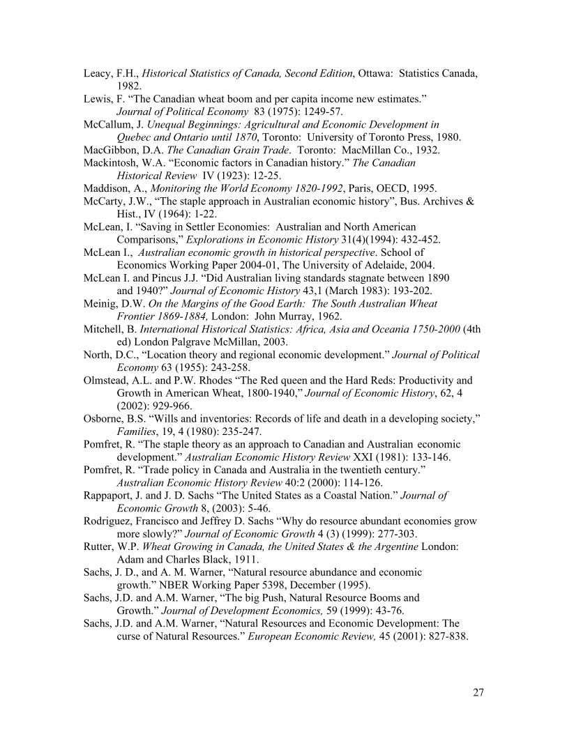
After converting the wealth in both data sets into U.S. dollars, the average wealth
in South Australia probated decedents was roughly 15 times greater than that of probated
decedents in the Thunder Bay District (Figures 1 and 2). Even if we doubled average
wealth for the Thunder Bay District in each year to account for the average age
differences across the two regions, the average wealth of South Australians would still be
massively larger (see footnote 47). SA wealth levels were higher than TB District in 1905
suggesting that much of that wealth was in place at the start of the period under study as
opposed to accumulated over the period. One interpretation is that some of this initial
difference in wealth levels reflects SA’s development through its earlier copper, wool and
wheat export periods in the nineteenth century. The higher wealth levels for South
Australia also reflect prolonged accumulation and growth over a longer period of time
prior to 1905, the results of an older population relative to TBD, as well as the possibility
that more of the benefits of the wheat economy were retained relative to the Thunder Bay
District. As well, there was inflation in asset values in Australia in the late 19th century
that could also explain substantially higher levels of wealth.53 The values of these assets
increased 1870-1890; fell somewhat to the mid 1890s but had high levels by 1905.54 In
addition, some of the difference in wealth levels could also be ascribed to differences in
the distribution of ages of the populations in the two regions. The Thunder Bay region
was newly settled and had a younger average age than South Australia.
53 Bentick “Foreign borrowing and wealth consumption”, McLean “Saving in Settler Economies”. 54 Another possibility is that differences in extraction methods have resulted in quite different samples being taken from the probate records. For Thunder Bay district, all estates probated between 1905 and 1915 have been included. In the case of South Australia, we have a stratified random sample being used. While selecting estates over 20000 pounds, the process also identified those leaving little wealth. While there may be differences in the proportion of estates of different sizes between the two samples, there is no obvious bias of either data set to its relative population.

19
The higher overall levels of wealth of South Australia could be ascribed to
endowments, linkage effects and timing. As a check, a comparison of the changes in
wealth levels across the two economies over 1905 to 1915 allows us to identify the
conditions and factors that result in natural resource exports developing an economy. If
SA’s capacity to accumulate wealth exceeds that of Thunder Bay over 1905 to 1915, then
the reasons for successful resource export based development are to be found in factors
specific to SA, such as its coastal ports. On the other hand, if there is no difference
between the capacities to accumulate wealth across the two economies over the same
period, then the reasons for successful resource export based development are to be found
in factors specific to the earlier period, when Ontario also successfully developed through
wheat exports.
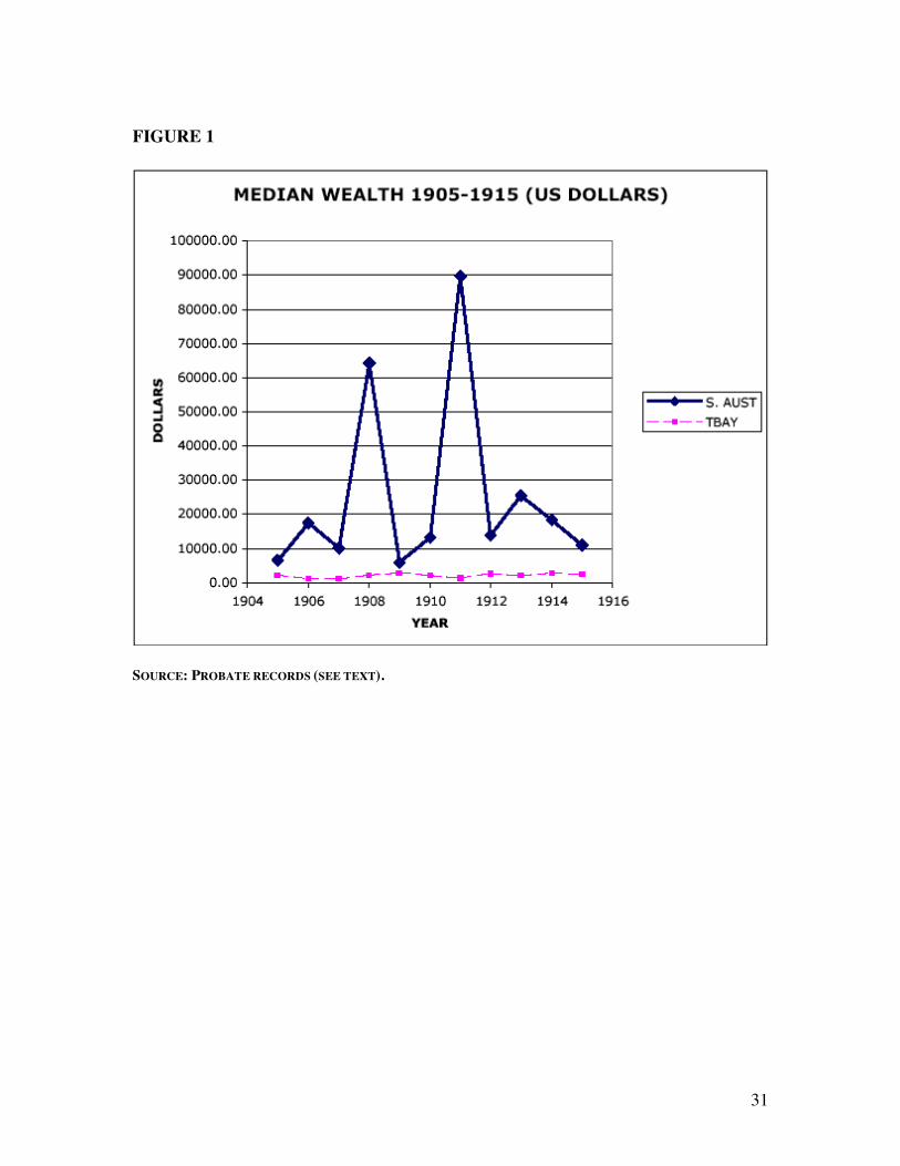
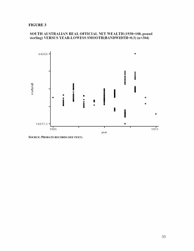
As mentioned above, one of the difficulties that we have encountered in assessing
the change in average wealth levels are the relatively high values for SA wealth in 1908
and 1911, which we believe could also partly be the result of having relatively fewer
observations for the SA sample in some years. Figures 3 and 4 plot LOWESS smoothes
of the value of real wealth in South Australia and Thunder Bay District.55 The LOWESS
smoothes help deal with the impact of extreme observations in assessing the wealth
profile over time. These figures suggest that this boom period for both economies
reached a peak in 1913 with the decline in wealth after 1913 ascribed to adjustments to a
post-boom equilibrium. Figure 5 further adjusts for the impact of outliers on wealth by
removing the top and bottom estate and recalculating the average for each year and then
normalizes the annual value by the average for 1905 to 1915 for the regional economy.
The results suggests that the changes in wealth levels over the period, particularly from
1905 to the peak value in 1913, are the same.
Table 2 shows the proportion of probated decedents reporting financial assets and
real estate across the two regions. These comparisons are important in allowing us to
infer whether the final forms in which income was accumulated either potentially
contributed to investment or detracted from it. The differences in the proportion reporting
55 LOWESS stands for Locally Weighted Scatterplot Smoothing and is a non-parametric smoothing technique. For South Australia, the CPI index with 1939=100 (Source: Mitchell International Historical Statistics) was used while the Altman adjusted Urquhart Index was used for the Thunder Bay data. Not all of the South Australian data had a year date and therefore the size of the data set was reduced to n=304.

20
real estate ownership were much smaller across the two regions whereas there is a very
large gap in financial asset ownership. Figure 6 shows the value of real estate in each
year normalized by the average value of real estate for the period 1905 to 1915. This
figure suggests that the value of “local assets” in the two economies had common
changes. The common changes in real estate ownership trends and values and the greater
importance of financial wealth for the South Australian decedents suggests that members
of the South Australian small open economy had the potential to be capital exporters by
1905.56 The importance of financial assets in the portfolio would also suggest that SA is
an example of what needs to happen for resource exports to generate sustainable income
levels according to Rodriguez and Sachs (1999).
The fact that the increase in average wealth was common to both economies
despite the much greater level of grain trade activity in TBD suggests that there are
features of the SA economy that allowed it to capture a greater share of the economic
rents/linkages associated with the rural economy. We also suspect, following McCallum
(1980) that these characteristics are shared with Southern Ontario from 1840 to 1870.
Two potential explanations need to be considered. First is the coastal location of the port
of Adelaide compared to the inland entrepot location of TBD. To the extent that total
resource costs of transporting grain to market were lower in SA than from the prairie
grain economy, there may have been more surplus to be captured by producers and
transporters. Second, it may be important who captured the surplus and how they
captured it. We characterize this latter point as a modification of a Stolper-Samuelson
theorem argument where a relative increase in the price of a commodity will increase the
real return to the factor used intensively in that industry and reduce the real return to the
other factor, but where that increase in real return ultimately remains depends on the
location of the owner of the factor of production.
To demonstrate the reasons for South Australia’s ability to generate the same
average change in wealth as the Thunder Bay District despite having total bushels of
wheat produced that represented at most 4 percent of total bushels of wheat shipped
through the Lakehead, we provide the following exercise. The role of the Thunder Bay
District in the Canadian Grain trade was to handle enormous quantities of grain arriving 56 See McLean “Saving in Settler Economies” Figure 4.

21
by rail from western Canada. The grain was transferred from rail cars, weighed,
inspected, and stored in terminal elevators before being transferred to a lake freighter.
The costs of doing these functions were on the order of 1.5 to 2 cents per bushel.57 As
much of the elevator capacity at the Lakehead (80 percent in 1905 and 60 percent in
1915) was owned by the railways, a large portion of this income would not have been
retained by the Lakehead region. Only the Paterson Elevators had its private owners
based in the Lakehead. In addition, the income of farmers from wheat production would
accrue to the prairie provinces, not the Thunder Bay District. The income earned by the
railways that brought the grain to the Lakehead, other than the wage payments to locally
based employees, would accrue to the location of the railway’s head office in the east of
the country as would the income earned by the companies that owned the ships that plied
the great lakes. We estimate the income from the wheat activities at the Lakehead
District as the number of bushels of wheat shipped from the Lakehead each year shown
in Figure 7, multiplied by 1.5 cents per bushel for years 1905 to 1915.
For the South Australian economy, we are looking at a situation where
production, transportation to the ocean port and handling were all carried out in the SA
economy. As we noted earlier, the SA rail network was state owned. Under the strong
assumption that the income for these activities was completely captured by local
producers, shippers and handlers, we approximate the income from a bushel of wheat for
the South Australian economy by the price of wheat in England less the cost of ocean
transportation from Australia. The average market price of an Imperial Bushel of wheat
at Pt. Adelaide was 0.19 of a Pound for 1905 to 1914.58 If we value the pound in US
dollars (an average of approximately 4.85 over the years 1905-1915), the price per bushel
of wheat was roughly equivalent to 90 cents. The total wheat income for South Australia
is thus approximated as the annual number of bushels of wheat produced time 90 cents
per bushel.59
57 Based on estimated costs of moving a bushel of wheat from Saskatchewan to Liverpool in 1925, Kerr and Holdsworth Historical Atlas of Canada Plate 19 “The Grain Handling System”. Rutter Wheat Growing in Canada provides a similar estimate for 1900-1910. 58 The price of wheat in Port Adelaide was 0.33 of a Pound in 1915, substantially higher than any other price over the period. The average price of a bushel of wheat in Port Adelaide is 0.2 of a Pound if this 1915 observation is included. 59 The issue of the level of freight rates or prices received by farmers is not relevant to this calculation so long as wheat production is not too supply elastic. Those rates and prices pertain to the distribution of the

22
Figure 8 demonstrates that despite a vast difference in quantities of grain
produced, transported and traded, wheat exports generated substantially higher income in
SA than TBD before 1910, and the convergence in grain trade incomes only takes place
after 1910 when grain shipments through the Lakehead increased substantially. Our
estimates of wheat incomes for the two economies provide a clear explanation for the
higher average wealth levels in SA relative to TBD, and the changes in wheat incomes
generally reflect the changes we demonstrate in average wealth in the two economies
over 1905 to 1915. For the Thunder Bay District, this estimated income from the wheat
trade shows the same approximate pattern as the average wealth estimates in Figure 5.
This comparison highlights a key determinant for successful development from
the export of natural resources; the ability to retain linkages associated with the resource
exports. One way to think of our comparison of these two wheat exporting economies is
that South Australia represents an economy where transportation, production and
handling of wheat is carried out by local owners of capital so that capital’s share of
income is retained locally. Thunder Bay District in contrast, is akin to a resource
exporting country where production and transportation functions are controlled by
external capital and that income does not remain in the local economy.60 While wheat
exports would have increased the incomes of farmers, transportation companies and other
sectors across Canada, the regional benefits of the grain trade would have been
distributed according to the home address of the head offices and the owners of capital.
As a consequence, much of the income and wealth generated by the resource exports did
little for the TBD economy.
The wealth data can also provide some insight into how much capital income may
have been exported out of each region. It is possible to classify the components of wealth
as locally held versus externally held. For the Thunder Bay District for example, life
insurance, stocks, securities, and cash in bank accounts would be the obvious externally
held assets with the remainder as internally held. For the period 1905 to 1909, the
wheat income across activities and agents involved in the production and trade of wheat. So long as all of these agents reside in the domestic economy, then the price of wheat at the port represents the income per unit of quantity for the domestic economy. 60 It should be noted that this characterization is still relevant today with the region referred to as a resource extraction colony. See Ibbitson “A new province called Mantario?” The Globe and Mail, August 9th, 2006, p. A4.

23
average value of internal assets was 4800 dollars while external assets averaged 2216
dollars. Between 1909 and 1915, internal assets rose to 9939 dollars – the growth
magnified by the boom in real estate values - while external assets rose to only 2282
dollars. For the 1905-1909 period, the share of externally held assets accounted for about
one-third of wealth and then declined to about one-fifth during the intense boom phase.
If real estate is removed from wealth, then the external share is 55 percent from 1905-
1909 and then declines to 37 percent from 1910 to 1915. For South Australia between
1905 and 1915, the share of assets held externally was just over one-third and for 1910 to
1915 this rose to just over 40 percent.61 When real estate is omitted the share of assets
held externally was over half in the first five years, rising to 63 percent in 1910 to 1915.
CONCLUSION
In this paper, we find that natural resources can result in successful economic
development in both the short run and the long run. The wheat boom of the early
twentieth century led to similar changes in wealth in the Thunder Bay District and in
South Australia suggesting successful short term impacts of the wheat boom across
regions. At the same time, the level of wealth was substantially higher in South Australia
than the Thunder Bay District suggesting that the wheat boom certainly generated
successful long-term economic development in South Australia. Moreover, wealth
distribution in Thunder Bay Distrcit was slightly more unequal than South Australia.
There are other important differences between the two regions. South Australia
benefited from earlier resource export episodes whereas in 1905 the Lakehead was really
a new economy. Adelaide SA is a coastal port that, for much of the latter nineteenth
century was a direct gateway to the world grain market, whereas the Port Arthur/Fort
William port was an intermediate terminus on the Canadian transportation system, as
grain was transferred from Great Lakes freighters to ocean going vessels. Adelaide
managed to maintain more of a hold on its hinterland region than did the Lakehead,
which faced substantial competition from other ports. Nevertheless, the Lakehead
61 This assumes real estate is included in total wealth.

24
experienced similar growth rates in wealth because of the much higher volume of grain
produced in Canada and shipped through the Lakehead relative to Adelaide.
While average wealth levels in SA between 1905-1915 were substantially higher
in SA than in the TBD, the increase in average wealth levels was equivalent in SA and
the Lakehead district. The volume of wheat passing through the Lakehead was
substantially greater than that produced in SA but SA was able to appropriate more
linkages from grain production. The higher wealth levels in SA relative to the TBD
during the 1905-1915 period were also likely caused by SA being a region of older
settlement and earlier wealth accumulation was compounded into higher levels relative to
the more newly settled TBD. Moreover, South Australia had greater control over its
institutions especially prior to 1901 when it was actually able to pursue its own tariff and
commercial policy.
Long term economic development from natural resources is likely a function of
the ability to retain linkages from the resource activity as well as the passage of time
necessary for linkages to develop and wealth to accumulate. The failure of the Thunder
Bay District by the late twentieth century to develop successful self-sustaining long run
economic growth and export capital as South Australia began to do in the early twentieth
century lay in the key differences in linkage generation and retention between the two
regions. The key to capturing the linkages from natural resource production is to
eventually generate domestic sources of capital rather than rely on external sources.
Our comparison suggests that an understanding of the apparent poor performance
of resource abundant economies may have less to do with the intrinsic properties of
natural resources and more to do with the sources and ownership of capital used to
produce and transport the natural resources to market. The implication for modern oil
producing nations is that they may be less likely to succeed in breaking from staples
dependent development in the long term when capital intensive production and
transportation of the commodity is combined with heavy reliance on external capital.

25
REFERENCES Altman, M “Staple theory and export-led growth: constructing differential growth.” Australian Economic History Review 43 (3) (2003): 230-255. Anderson, F.J. “Regional trade and adjustment with expenditure effects.” Canadian Journal of Regional Science XIV (1991): 23-46. Anderson, F.J. Regional Economic Analysis A Canadian Perspective. Toronto: Harcourt Brace Jovanovich 1988. Auty, R. M. “The Political Economy of Resource-Driven Growth,” European Economic
Review 45 (4-6) (2001): 839-846. Baldwin, R.E. “Patterns of development in newly settled regions.” Manchester School of Economic and Social Studies XXIV (1956): 161-179. Bentick, B.L. “Foreign borrowing and wealth consumption: Victoria 1873-93,”Economic
Record, 45(111) (1969): 415-431. Bertram, G.W. “The relevance of the wheat boom in Canadian economic growth.” Canadian Journal of Economics VI (1973): 545-566. Buckley, K.A.H. “The role of staple industries in Canada's economic development.” The Journal of Economic History 18 (1958): 439-450. Butlin N.G., Investment in Australian Economic Development 1861-1900, Department of Economic History, ANU. Canberra, 1964[1976]. Callender, G.S. “The early transportation and banking enterprises of the states in relation to the growth of corporations.” Quarterly Journal of Economics XVII (1902): 111-162. Callender, G.S. Selections from the economic history of the United States, 1765-1860. New York: Augustus M. Kelley 1965[1909]. Caves, R.E.“’Vent for surplus’ models of trade and growth.” In Trade, growth and the
balance of payments: Essays in honor of Gottfried Haberler. Baldwin et al., 95-115, Chicago: Rand McNally, 1966.
Caves, R.E. “Export-led growth and the new economic history.” In Trade, Balance of Payments and Growth, edited by Bhagwati et al., 403-442, Amsterdam: North Holland, 1971.
Chambers, E.J. and D.F. Gordon, “Primary products and economic growth: An empirical measurement.” Journal of Political Economy 74 (1966): 315-331. Corden, W.M. and J.P. Neary “Booming sector and de-industrialization in a small open economy,” Economic Journal 92 (1982): 825-848. Corden, W.M. “The economic effects of a booming sector.” International Social Science Journal 35 (1983): 441-454. Crafts, N. “Globalisation and Economic Growth: A Historical Perspective,” World
Economy (2004): 45-58. Dales, J.H., J.C. McManus and M. Watkins, “Primary products and economic growth: A comment.” Journal of Political Economy 75 (1967): 876-880. Di Matteo, L. (2004) “Wealth and inequality on Ontario’s Northwestern Frontier:
Evidence from Probate” Histoire Sociale-Social History 38: 75, 79-104. Di Matteo, L. “The economic development of the Lakehead during the wheat boom era:1900-1914.” Ontario History LXXXIII (1991): 297-316.

26
Di Matteo, L. “Evidence on Lakehead economic activity from the Fort William building permit registers, 1907-1969.” Papers and Records, Thunder Bay Historical Museum Society XX (1992): 37-49. Di Matteo, L. “Booming Sector Models, Economic Base Analysis, and Export-Led
Development: Regional Evidence from the Lakehead.” Social Science History 17 (4) (1993): 593-617.
Di Matteo, L. “The Effect of Religious Denomination on Wealth: Who Were the Truly Blessed? Social Science History 31 (3) (2007): 299-341.
Di Matteo, L. and P. George “Canadian wealth Inequality in the Late Nineteenth Century: A Study of Wentworth County Ontario, 1872-1902,” Canadian Historical Review 73 (4) (1992): 453-483.
Dunsdorfs, E. The Australian wheat-growing industry 1788-1948. The University Press, Melbourne 1956. Fogarty, J. “Economic history and the limits of staple theory.” In Clio's Craft edited by T. Crowley: 179-194, Toronto: Copp Clark Pitman, 1988. Fowke, V.C. The National Policy and the Wheat Economy. Toronto: University of Toronto Press, 1971[1957]. Gallup, J.L., J. D. Sachs and A.D. Mellinger “Geography and Economic Development.”
NBER Working Paper Series, Working Paper 6849, 1998. Harley, C. K. “Western Settlement and the Price of Wheat, 1872-1913,” Journal of
Economic History 38 (4) (1978): 865-878. Harley, C. K. “Transportation, the World Wheat Trade, and the Kuznets Cycle, 1850-
1913,” Explorations in Economic History 17 (1980): 218-250. Harley, C.K. “Resources and economic development in historical perspective”. In Responses to Economic Change, Royal Commission on the Economic Union and Development Prospects for Canada, Vol. 27 edited by David Laidler Toronto: University of Toronto Press. 1986: 1-32. Harley, C.K. “Comments on factor prices and income distribution in less industrialized
economies 1870-1939: Refocusing on the frontier”, Australian Economic History Review 47 (3) (2007): 238-248.
Hartwick, J. “Investment of rents from exhaustible resources and intergenerational equity”, American Economic Review. 67 (5) (1977): 972-974.
Hirst, J.B., Adelaide and the Country 1870-1917. Their Social and Political Relationship, Melbourne: Melbourne University Press 1973. Howell, A. The Law and Practice as to Probate, Administration and Guardianship in
Surrogate Courts. Toronto: Carswell 1880. Hughes, J.and L.P. Cain, American Economic History Fourth Edition. New York: Harper
Collins, 1994. Innis, H.A. The Fur Trade in Canada: An Introduction to Canadian Economic History. Toronto: University of Toronto Press 1984[1930]. Innis, H.A. The Cod Fisheries: The History of an International Economy.Toronto: University of Toronto Press 1978[1940]. Innis, H.A. Essays in Canadian Economic History. Mary Q. Innis (ed.) Toronto: University of Toronto Press 1969[1956]. Kerr, D. and D. W. Holdsworth eds. Historical Atlas of Canada, Volume III: Addressing
the Twentieth Century 1891-1961, Toronto: University of Toronto Press, 1990.
27
Leacy, F.H., Historical Statistics of Canada, Second Edition, Ottawa: Statistics Canada, 1982.
Lewis, F. “The Canadian wheat boom and per capita income new estimates.” Journal of Political Economy 83 (1975): 1249-57. McCallum, J. Unequal Beginnings: Agricultural and Economic Development in Quebec and Ontario until 1870, Toronto: University of Toronto Press, 1980. MacGibbon, D.A. The Canadian Grain Trade. Toronto: MacMillan Co., 1932. Mackintosh, W.A. “Economic factors in Canadian history.” The Canadian Historical Review IV (1923): 12-25. Maddison, A., Monitoring the World Economy 1820-1992, Paris, OECD, 1995. McCarty, J.W., “The staple approach in Australian economic history”, Bus. Archives & Hist., IV (1964): 1-22. McLean, I. “Saving in Settler Economies: Australian and North American Comparisons,” Explorations in Economic History 31(4)(1994): 432-452. McLean I., Australian economic growth in historical perspective. School of Economics Working Paper 2004-01, The University of Adelaide, 2004. McLean I. and Pincus J.J. “Did Australian living standards stagnate between 1890 and 1940?” Journal of Economic History 43,1 (March 1983): 193-202. Meinig, D.W. On the Margins of the Good Earth: The South Australian Wheat Frontier 1869-1884, London: John Murray, 1962. Mitchell, B. International Historical Statistics: Africa, Asia and Oceania 1750-2000 (4th
ed) London Palgrave McMillan, 2003. North, D.C., “Location theory and regional economic development.” Journal of Political
Economy 63 (1955): 243-258. Olmstead, A.L. and P.W. Rhodes “The Red queen and the Hard Reds: Productivity and
Growth in American Wheat, 1800-1940,” Journal of Economic History, 62, 4 (2002): 929-966.
Osborne, B.S. “Wills and inventories: Records of life and death in a developing society,” Families, 19, 4 (1980): 235-247.
Pomfret, R. “The staple theory as an approach to Canadian and Australian economic development.” Australian Economic History Review XXI (1981): 133-146. Pomfret, R. “Trade policy in Canada and Australia in the twentieth century.” Australian Economic History Review 40:2 (2000): 114-126. Rappaport, J. and J. D. Sachs “The United States as a Coastal Nation.” Journal of
Economic Growth 8, (2003): 5-46. Rodriguez, Francisco and Jeffrey D. Sachs “Why do resource abundant economies grow
more slowly?” Journal of Economic Growth 4 (3) (1999): 277-303. Rutter, W.P. Wheat Growing in Canada, the United States & the Argentine London:
Adam and Charles Black, 1911. Sachs, J. D., and A. M. Warner, “Natural resource abundance and economic growth.” NBER Working Paper 5398, December (1995). Sachs, J.D. and A.M. Warner, “The big Push, Natural Resource Booms and Growth.” Journal of Development Economics, 59 (1999): 43-76. Sachs, J.D. and A.M. Warner, “Natural Resources and Economic Development: The curse of Natural Resources.” European Economic Review, 45 (2001): 827-838.

28
Schedvin, C.B. “Staples and regions of Pax Britannica.” Economic History Review 2nd ser XLIII 4 (1990): 533-559. Shanahan, M.P. “The distribution of personal wealth in South Australia 1905-1915” Australian Economic History Review (September) XXXV: 2 (1995): 82-111. Shaw, A.G.L. The Story of Australia, London: Faber, 1954. Sinclair W.A., The process of economic development in Australia, Melbourne: Longman
Cheshire, 1976 [1985]. Stafford, J. “A Century of Growth at the Lakehead” In Thunder Bay: From rivalry to
unity edited by T. Tronrud and A.E. Epp, Thunder Bay: Thunder Bay Historical Museum Society, 1995.
Stevenson, T. “Population Statistics”. In South Australian Historical Statistics, edited by Vamplew W., Richards E., Jaensch D., and J.Hancock, Monograph No 3, University of New South Wales Sydney, 1986. Urquhart, M.C. “New estimates of gross national product, Canada, 1870-1926: Some
implications for Canadian development.” In NBER Studies in Income and Wealth vol. 51: Long Term Factors in American Economic Growth edited by S.L. Engerman and R.E. Gallman Chicago: University of Chicago Press: 1986, 9-94.
Urquhart, M.C. Gross National Product, Canada, 1870-1926: The Derivation of the Estimates. McGill-Queens University Press, 1994.
Vamplew W., Richards E., Jaensch D., and Hancock J. South Australian Historical Statistics, Historical Statistics Monograph No 3. University of New South Wales History Project Incorporated 1988.
Vamplew W. (ed.) Australians. Historical Statistics, Sydney: Fairfax, Syme &Weldon Associates, 1987. Wagg, P. “The bias of Probate: Using Deeds to Transfer Estates in Nineteenth-Century
Nova Scotia,” Nova Scotia Historical Review 10 (1) (1990): 74-87. Watkins, M.H. “A staple theory of economic growth.” Canadian Journal of Economics and Political Science XXIX (1963): 141-158. Wright, G. and J. Czelusta, “Why economies slow: the myth of the resource curse,”
Challenge 47 (2004): 6-38.

29
TABLE 1: WHEAT PRODUCTION IN SOUTH AUSTRALIA AND CANADA
AREA UNDER WHEAT (ACRES) Year SA Australia Canada 1870 604761 1123839 1647000 1880 1733542 3052617 2367000 1890 1673573 3228535 2701000 1900 1913247 5666614 4225000 1910 2104719 7372456 8865000 1915 2739214 12484512 15109000 WHEAT PRODUCTION (BUSHEL PER ACRE) Year SA Canada 1870 11.50 10.20 1880 5.00 13.70 1890 5.60 15.60 1900 5.90 13.20 1910 11.60 14.90 1915 12.50 26.00 SOURCE: CANADA-HISTORICAL STATISTICS OF CANADA DUNSDORFS (1956) APPENDIX; VAMPLEW ET AL (1987) AG46-54.

30
TABLE 2: ASSET HOLDING PROPORTIONS Year Real Estate Financial Assets S. Aust T. Bay S. Aust T. Bay
1905 0.68 0.87 0.92 0.73 1906 0.85 0.58 0.94 0.67 1907 0.72 0.59 0.84 0.77 1908 0.75 0.62 0.96 0.81 1909 0.79 0.76 0.95 0.71 1910 0.73 0.70 0.95 0.66 1911 0.83 0.72 0.97 0.53 1912 0.82 0.69 0.95 0.64 1913 0.74 0.69 0.97 0.64 1914 0.84 0.74 1.00 0.69 1915 1.00 0.81 0.83 0.68
Average 0.79 0.70 0.95 0.67
SOURCE: PROBATE RECORDS (SEE TEXT).
31
FIGURE 1
SOURCE: PROBATE RECORDS (SEE TEXT).

32
FIGURE 2
SOURCE: PROBATE RECORDS (SEE TEXT).
33
FIGURE 3
SOURCE: PROBATE RECORDS (SEE TEXT).

34
FIGURE 4
SOURCE: PROBATE RECORDS (SEE TEXT).

35
FIGURE 5 COMPARISON OF NORMALIZED WEALTH AFTER ADJUSTING FOR EXTREME OBSERVATIONS EACH YEAR*
*BOTTOM AND TOP ESTATE DROPPED FOR EACH YEAR TO ESTIMATE AN OUTLIER ADJUSTED AVERAGE WEALTH FOR EACH YEAR. THIS IS NORMALIZED BY THEN DIVIDING EACH YEAR BY THE AVERAGE FOR THE WHOLE 1905-1915 PERIOD. SOURCE: PROBATE RECORDS (SEE TEXT).
"Normalized" Adjusted Wealth
0.00
0.20
0.40
0.60
0.80
1.00
1.20
1.40
1.60
1.80
1905 1907 1909 1911 1913 1915
Year
S.AUST
TBAY

36
FIGURE 6 COMPARISON OF NORMALIZED* REAL ESTATE
* NORMALIZED BY DIVIDING EACH YEAR BY THE AVERAGE FOR THE WHOLE 1905-1915 PERIOD. SOURCE: PROBATE RECORDS (SEE TEXT).
"NORMALIZED" REAL ESTATE
0
0.5
1
1.5
2
2.5
3
1905 1907 1909 1911 1913 1915
YEAR
S.Aust
T.Bay

37
FIGURE 7
Total Grain Shipments from the Lakehead: 1905-1929
0
50000000
100000000
150000000
200000000
250000000
300000000
350000000
400000000
450000000
1905
1906
1907
1908
1909
1910
1911
1912
1913
1914
1915
1916
1917
1918
1919
1920
1921
1922
1923
1924
1925
1926
1927
1928
1929
Year
Bushels
Source: Canal Statistics, Department of Railways and Canals and Dominion bureau of Statistics, Statistics Canada, 54-201 (1919-1931); Canada Year book (pre 1919).

38
FIGURE 8
Estimated Gross Incomes From Wheat Production, Transportation and Trade, The Lakehead
and South Australia, 1905-1915
0
500000
1000000
1500000
2000000
2500000
3000000
1905 1906 1907 1908 1909 1910 1911 1912 1913 1914 1915
Do
llars Lakehead
SA
SOURCE: AUTHORS CALCULATIONS (SEE TEXT)


