
HAL Id: halshs-00180128https://halshs.archives-ouvertes.fr/halshs-00180128
Preprint submitted on 17 Oct 2007
HAL is a multi-disciplinary open accessarchive for the deposit and dissemination of sci-entific research documents, whether they are pub-lished or not. The documents may come fromteaching and research institutions in France orabroad, or from public or private research centers.
L’archive ouverte pluridisciplinaire HAL, estdestinée au dépôt et à la diffusion de documentsscientifiques de niveau recherche, publiés ou non,émanant des établissements d’enseignement et derecherche français ou étrangers, des laboratoirespublics ou privés.
Life-cycle position and migration to urban and ruralareas: estimations of a mixed logit model on French data
Cécile Détang-Dessendre, Florence Goffette-Nagot, Virginie Piguet
To cite this version:Cécile Détang-Dessendre, Florence Goffette-Nagot, Virginie Piguet. Life-cycle position and migrationto urban and rural areas: estimations of a mixed logit model on French data. 2004. �halshs-00180128�

GATE Groupe d’Analyse et de Théorie
Économique UMR 5824 du CNRS
DOCUMENTS DE TRAVAIL - WORKING PAPERS
W.P. 04-03
Life-cycle position and migration to urban and rural areas: estimations of a mixed logit model on French data
Cécile DETANG-DESSENDRE
Florence GOFFETTE-NAGOT
Virginie PIGUET
Avril 2004
GATE Groupe d’Analyse et de Théorie Économique UMR 5824 du CNRS
93 chemin des Mouilles – 69130 Écully – France B.P. 167 – 69131 Écully Cedex
Tél. +33 (0)4 72 86 60 60 – Fax +33 (0)4 72 86 60 90 Messagerie électronique [email protected]
Serveur Web : www.gate.cnrs.fr

Life-cycle position and migration to urban and rural areas:
estimations of a mixed logit model on French data1
Cécile Détang-Dessendre
CESEAR-INRA2
Florence Goffette-Nagot
GATE-CNRS3
Virginie Piguet CESEAR-INRA4
Abstract: Migration flows between urban and rural areas in developed countries show a strong
difference in migration destinations with regard to age. Our paper analyses, in the French
case, who rural areas attract or repel and what their so-called “pull-factors” are. Our goal is to
explain the propensity to migrate and the destination choice among four categories of area
(urban centres, suburbs, rural areas under urban influence, rural LMAs), for three age groups.
Mixed logit models, that do not rely on the IIA assumption and allow for heterogeneity in
individual behaviours are estimated on a large French sample. The results show that the
educational level of young people and the labour market characteristics of their initial
residential area particularly influence their destination choices. The labour market variables
have little influence on the migration decisions of the middle-aged, for whom residential
motivations appear to be predominant. The migration decisions of 45-64 years old are clearly
residentially motivated changes.
Keywords : Migration, Life-cycle, Urban and rural areas, mixed logit models.
JEL Classification Codes : J62, R23.
1 The authors would like to thank Pierre Blanchard, Claude Montmarquette and Bertrand Schmitt for their
constructive comments. This paper was presented at the XVII Annual Conference of the European Society for
Population Economics (New York, 2003).
2 CESEAR-INRA, 26 bd docteur Petitjean, BP87999, 21079 Dijon Cedex, France, [email protected].
3 GATE, CNRS-Univ. Lyon 2-ENS, 93 chemin des Mouilles69130 Ecully, France, [email protected].
4 CESEAR-INRA, 26 bd docteur Petitjean, BP87999, 21079 Dijon Cedex, France, [email protected].
1

1. Introduction
The increase in the population of rural areas in developed countries in the 1970’s has been
considered by many as part of a “demographic revolution” (Beale, 1977; Vining, Strauss,
1977; Champion and Fielding, 1992). After a slowdown in the 1980’s, the last ten years of the
20th century showed again a dispersal pattern, supporting the idea of a “clear break” (Fuguitt,
Beale, 1996; Long, Nucci, 1997). In the USA, population in non-metropolitan areas grew
during the 1990s, due to high net immigration rates (Barkley, Henry, 1997; Hamrick, 2002;
U.S. Census Bureau, 2003). Most European countries are also experiencing a population
dispersal mainly explained by migration flows (see Geyer, 2002, for the presentation of
various recent situations in developed countries). In France, the rural population increased by
0.2 % per annum between 1990 and 1999, largely due to a positive migration balance (+ 0.4
% per annum5) (INRA, INSEE, 1998; Bessy-Piétry et al., 2000).
The demographic growth of rural areas has implications in terms of public policies, as
migratory flows affect strongly not only population densities, but also the demographic
composition of rural populations. In the USA, one issue at moment is the ageing of population
in non-metropolitan areas, as the rural birth rate is low and elderly represent a large part of the
migration flows to rural areas (Rogers, 2002). Urban sprawl is also a topic of debate
(Brueckner, 2000; Carruthers, Ulfarsson, 2002). In France, the dramatic increase in rural
population raises concerns about the provision of public services and facilities, and the
heterogeneity of economic development between urban and rural areas is considered as
undesirable. As a result the French government explicitly raises the issue of “developing rural
areas” in a bill that was proposed at the beginning of September 2003 (Ministère de
l’Agriculture, 2003). Its main objectives are (i) sustaining economic activities, (ii) improving
access to public facilities, and (iii) ensuring environmental respect. These propositions rest on
the idea that “it is socially preferable to lead activities to people than people to activities. This
conception is opposite to that of Anglo-Saxon countries where incentives are directed towards
migrations rather than relocation of activities” (Mougeot, Gérard-Varet, 2001).
5 The migration balance was of +0.23 % per annum between 1982 and 1990
2

In view of these two different conceptions, one might ask whether policies should not first
take into account the factors affecting urban-rural mobility. In particular, the strong difference
in migration destinations with regard to age calls for a better comprehension of what in rural
areas attracts or repels individuals depending on their age (Champion and Fielding, 1992).
Our paper contributes to this debate. More precisely, our objective is to analyse, in the French
case, who rural areas attract or repel and what their so-called “pull-factors” are. In other
words, we investigate why certain types of area are more suitable for people of certain ages
and how this variation in motives amongst different age groups affects migratory flows
towards rural areas. The expected results provide the basis for regional planning policies
focusing on individual mobility and individual migrant characteristics. As Nivalainen (2002)
outlines, this question has not received much attention in the micro level research.
In terms of general determinants, it is accepted that (i) rural areas adjacent to urban cores
attract households due to lower housing prices in the Alonso-Muth tradition (Miezskowsky,
Mills, 1993), (ii) more remote rural areas have natural amenities allowing their demographic
rebirth (McGranahan, 1999) and (iii) low-density areas may provide specific job opportunities
(Kontuly, 1998). More precisely, Bierens and Kontuly (2002) investigate whether regional
differentials in employment growth are a major determinant of the so-called
“counterurbanization”. However, their data are at the regional level and are therefore not
precise enough to deal with the heterogeneity of rural areas. Renkow and Hoover (2000) and
So et al. (2001) analyse commuting behaviour in metropolitan and non-metropolitan areas on
the basis of housing prices and wage differentials, the former with aggregate data and the
latter with micro level data. Rouwendal and Meijer (2001) make use of individual stated
preferences data in order to estimate preferences for housing, jobs and commuting. In these
studies however, empirical results show substitution patterns between housing and transport
prices, but do not give insights into the characteristics of rural immigrants. Nivalainen (2002)
gives a precise picture of who migrates to rural areas in Finland in recent times. Nonetheless,
the Finnish context is a bit specific in that migration rates are low in comparison with other
developed country, and the study period corresponds to a sudden recession in Finland.
Moreover, except Rouwendal and Meijer (2001) who allow for heterogeneity in preferences,
these analyses consider individual behaviour as homogenous in the population. On the
contrary, we argue that the factors affecting migration choices differ by age, as suggested by
the demographic structure of migration flows. As a consequence, we implement an empirical
3

model that stresses differentiation by age by estimating separate models for three age classes,
while allowing for heterogeneity into each class with the use of a mixed logit model.
The other main characteristic of our analysis is to take into account not just one type of rural
areas, but several categories along an urban-rural gradient. This view is in accordance with
operational classifications used for instance in the USA, where the urban-rural continuum
code captures a similar idea. Here, we consider that locations along the urban-rural gradient
can be characterised along two dimensions. The first one is the type of labour market area
(LMA hereafter) to which the locality belongs, while the second one is the distance to the
employment centre of this LMA. More precisely, we distinguish urban and rural LMAs
depending on the size of their employment centre, and then consider three classes in urban
LMAs: urban centres, suburban areas and rural areas under urban influence which can be seen
as more remote suburbs (see definitions in appendix 1). According to economic geography
and urban economics, the type of LMA induces differentiation in the working of labour
markets, while distance to the centre governs the working of land and housing markets. These
differentiations suggest some hypotheses concerning the main determinants of migration
destinations for three age classes.
In order to test this set of hypotheses, we estimate mixed logit models on a French sample
taken from the “Echantillon Démographique Permanent” (Permanent Demographic Sample)
which is a source allowing for the monitoring of a set of individuals from one census to the
next (here 1982-1990). Our goal is to explain the propensity to migrate and the destination
choice among four categories of area (urban centres, suburbs, rural areas under urban
influence, rural LMAs), for three age groups. Explanatory variables are individual
characteristics related to labour market or housing demand, such as gender, marital status,
evolution of household size, educational level or rise in social status, as well as some
attributes of the initial location in terms of amenities or the unemployment rate.
The results show that the determinants of migration decisions and destination choices vary, as
assumed, with age range. The educational level of young people and the labour market
characteristics of their initial residential area particularly influence their destination choices.
On the contrary, the labour market variables have little influence on the migration decisions of
the middle-aged, for whom residential motivations appear to be predominant. In this group,
changes in family composition influence strongly migration decisions, reflecting the
4

consequences of housing demand, and the first access to homeownership has a strong
influence on migration towards suburban areas and rural areas under urban influence. Also, a
rise in the social status of the middle-aged is associated with migration to urban LMAs.
Finally, the migration decisions of 45-64 years old are clearly residentially motivated
changes. Some migration is predominantly directed towards rural areas: this is the case for
people whom children leave, for retired individuals, and also for individuals residing in 1982
in the Ile-de-France region.
In the next section, we present the economic mechanisms we hypothesise have governed the
migration choices between urban and rural areas in France in recent times. We then draw
consequences for the agent's choice of location. Section 3 presents the data and the
econometric method used to test these hypotheses. Some statistic evidence and the results of
the econometric estimations are shown in section 4. Section 5 summarises our findings and
sets out a few concluding remarks.
2. Migration along an urban-rural gradient: hypotheses
Let us recall that economic theory considers migration as resulting from the comparison of
utilities (actually discounted future flows of utility) provided by the different locations, after
deduction of the cost of migration. An individual gets a certain level of utility from each
location depending on his preferences and endowments and of the location characteristics in
terms of housing, amenities and the labour market. Migration occurs if the place that
maximises net utility differs from the current location (Greenwood, 1997).
The individual's preferences and endowments change over time and in particular with his life-
cycle position. The influence of position in the life-cyle on migration propensity has been
highlighted in various studies, for instance recently by Détang-Dessendre et al. (2002) or
Nivalainen (2004). Life-cycle position may also explain destination choices, with the
characteristics of different areas meeting the requirements of different categories of
population (Clark, Hunter, 1992). In the early years of the individual's working life,
professional motives far outweigh residential motives (attributes of housing and its
environment). The latter are likely to gain sway as the individual grows older and has a larger
5

family. By retiring age, one can suppose that they are the only motives remaining. These
observations suggest estimating migration destinations choices for different age groups, as
some mechanisms might totally differ at different life-cycle stages.
With regard to the areas, we emphasise that there is an urban-rural gradient defined following
two dimensions. The first one concerns belonging to a local labour market area. The working
of the labour market is supposed to vary according to the density of labour demand and
supply, and thus with whether the area belongs to an urban or rural LMA, with those two
possibilities being distinguished on the basis of their size in terms of employment. Secondly,
the housing market outcomes and residential characteristics vary within urban LMAs with
distance from the employment centre. The combination of these two dimensions leads us to
distinguish rural and urban LMAs and to consider three main categories within urban LMAs:
urban centres where the majority of jobs are located, suburbs that have good accessibility to
urban centres, and small peripheral localities, that can be qualified as rural areas under urban
influence, due to their strong commuting flows to the urban centre. The distinction by
distance from the centre being not relevant in the rural case, we consider only one category
within rural LMAs.
Consequently, the motives for migration are sought by comparing and contrasting the
characteristics of the different categories of area along the urban-rural gradient, alongside
individual attributes that vary in particular with age. Locational characteristics interact with
individual life-cycle position through two channels: (i) labour market related considerations
and (ii) housing related considerations.
2.1. Professional motivations of migration and type of LMA
According to economic geography, the size of LMA determines the functioning of the labour
market, in particular wages and the probability of unemployment that are the components of
expected income. Thisse and Zenou (1995) show that the higher density of labour supply and
demand makes for better matches in urban labour markets. Urban LMAs have a rapid
turnover in employment, and so offer better chances of finding work than rural labour
markets. On the contrary, turnover in employment is lower in rural LMAs and thus jobs are
steadier (Jayet, 1995). Hence, one can argue that the probability of finding a job is higher in
urban LMAs, all things being equal, and in particular for a given age and skill level.
6

Furthermore, a better quality of job-employee matches and urbanisation economies can
account for a higher productivity in urban LMAs, explaining higher urban wages.
As a consequence, one can suppose that expected income of a given individual is higher in
urban than in rural LMAs and that employment considerations should lead individuals to
migrate to urban LMAs. This is particularly true at the beginning of their career and justify
that we run separate estimations for young people, aiming at showing that they predominantly
migrate to urban LMAs and highlighting the characteristics of young migrants that are still
attracted by rural areas. Moreover, secondary job markets that are more developed in urban
areas are of importance for the professional integration of young women. Therefore, gender
should explain migration choices of the youngest.
Hamilton et al. (2000) argue that not only employment turnover and nominal wages are
higher in urban than in rural LMAs, but also the frequency of technological job opportunities.
Jayet (2000) analyses the difference between rural and urban LMAs, taking into account
spatial labour division: higher tertiary sector firms or high-tech industries locate in urban
LMAs, while firms using lower technological levels locate in rural LMAs. These analyses
suggest that the advantage of urban areas in terms of matching will be particularly decisive for
high-skilled workers, while low-skilled workers do not need to leave rural LMAs to find a
job. In accordance, the probability of being employed as well as wages rise with skill level
faster in urban than in rural areas. As a matter of fact, in 1998 in France, executives represent
23% of jobs in urban LMAs and 4% of those in rural LMAs, while blue collar workers
account for 55% of the latter and only 21% of the former (Gaigné, Goffette-Nagot, 2003).
Concerning wage differentials, executives earn on average 11% more in urban LMAs
compared to rural LMAs, while urban blue collar workers earn only 5% more than rural ones.
Finally, one can argue that there exists a spatial differential in expected income in favour of
urban areas, which increases with the worker’s skill level, explaining that migration towards
urban areas should be more profitable for educated workers. As a consequence, three
individual characteristics will be introduced in the estimations of migration decisions:
educational level, social category and social rise, the latter indicating whether the individual
changes social category in favour of a higher one (see variable definition in section 3) during
the observation period. Moreover, the unemployment rate in the initial location will be taken
into account, aiming at capturing whether a low employment probability in the initial location
7

pushes people towards urban LMAs. Finally, the effect of size of the initial LMA will be
more precisely taken into account through a variable interacting the population density of the
initial commune and the size of LMA (see table 1 for a summary of explanatory variables and
their definitions).
2.2. Residential motivations of migration and distance to the centre
Following urban economics, housing prices decrease with distance from an employment
centre and the choice of location distance within a LMA may be seen as resulting from the
trade-off between households’ land consumption and commuting cost (Fujita, 1989). This
mechanism is responsible for urban sprawl in large metropolitan areas, as observed both in the
United States since the 1950’s (Anas et al., 1998) and in Europe since the 1970’s (Champion,
1989). More precisely, the ratio between workers and non workers in a household influences
the choice of distance from the centre: the lower the weight of commuting costs compared to
housing needs, the farther away households locate from the centre. In terms of migration, this
means for instance that working households experiencing a rise in the number of their
children are likely to move to suburbs or rural areas under urban influence. More generally, a
decrease in the household size should encourage people to move to the centre and vice versa.
A particular role is played by homeownership in explaining moves towards the suburbs.
Actually, down payment constraints and mortgage interest make valuable the decrease in
housing price permitted by a location further away from the centre. In that respect, becoming
a homeowner may be powerful in explaining the choice of migrating to suburban areas or
rural areas under urban influence. This will be captured in our estimations by a specific
variable.
Moreover, the land rent curve is higher in an urban LMA than in a rural one, and, more
generally, land rents tend to rise with the size of the employment centre. As a matter of fact,
during the 1984-88 period, housing prices were about 20% lower in urban LMAs with a
centre having less than 200,000 inhabitants in their centre, and 40% cheaper in rural LMAs,
compared to urban LMAs with a centre of more than 200,000 inhabitants. Within each LMA,
prices were 7 to 9 percent lower in the suburbs than in the centre, depending on the LMA size
(INSEE, French Housing Survey, our own calculations). Therefore, migration towards the
suburbs is likely to be more frequent the bigger the LMA. Furthermore, this may account for
8

the frequent migration of retired households towards rural LMAs, as these households are no
longer tied to employment centres.
In addition, the fall in housing prices with distance from the city centre implies a similar fall
in density, and low densities are often associated with natural amenities such as quality
scenery or low pollution levels. This means that the level of natural amenities increases with
distance from the centre and that it is higher in rural than in urban LMAs for a given distance
from the centre. One knows that amenities influence the choice of location at a certain
distance from the city centre as a function of income, alongside the variation with income of
the value of commuting time and housing consumption (Diamond, 1980; Brueckner et
al., 1999). One can expect such considerations to explain destination choices of households,
in suburbs or in rural areas under urban influence, depending on their income and social
category. The impact of income level on distance from the city centre that results from these
several determinants cannot be known a priori, but the social category variable that enters our
estimations will be likely to give some insight into this question.
The density of the initial location, interacted with the LMA size will also be introduced,
aiming at capturing households’ demand for amenities. Furthermore, as the role of return
migration towards birth regions has often been highlighted in France, particularly among the
elderly, a variable assessing whether people are in 1990 in their birth département while they
were not in 1982 is used. Similarly, due to the particular migration behaviour of retirees from
the Paris region, a variable indicating whether people are located in the Ile-de-France region
in 1982 is also introduced. Both variables are likely to reflect situations where migration
towards rural areas in search of rural amenities are more frequent.
A summary of the impact of each explanatory variable and expected effects is found in
table 1.
[insert Table 1 about here]
9

3. Methods and data
The objective of the empirical analysis presented here is to test the hypotheses just formulated
about the explanatory mechanisms of migration choices along an urban-rural gradient. This
test involves showing the influence of individual and initial location characteristics on the
probabilities to move and to choose each type of area.
3.1. Data
The individual data used are from the Permanent Demographic Sample (hereafter PDS)
conducted by the French Institute for Statistics and Economic Studies (INSEE). PDS was first
set up in 1967. It concerns all individuals born each year within four reference days and
collates information relating to their civil status (births, marriages, etc.) and their census
returns for 1968, 1975, 1982 and 1990. The sample represents a little over 1% of the French
population and is an ideal tool for longitudinal demographic analyses (see Rouault, 1995, for
a more detailed presentation of PDS). It contains for each individual her characteristics, the
characteristics of her household and her commune of residence at each Census6. Our analysis
focuses on the period 1982-1990 and selects individuals aged 15 to 64 years in 1982. These
selection criteria and different technical constraints related to the source provide a sample of
77,845 individuals7.
We define migration as the commune of residence in 1990 being different from that in 1982
(changes of commune within an urban centre not being counted). 25% of our sample
(18,781 individuals) migrated between 1982 and 1990. The main limit of the definition of
migration we use is that it considers multiple migration, of which the probability is non
negligible over a period of eight years, as a single migration and that it ignores return
migration during the period between censuses.
6 Communes are French municipalities. They correspond to the lowest level of territory division in this country.
A quarter of the French population lived in 1990 in 31,251 rural communes and three quarters lived in 5,300
urban communes. Urban communes are grouped in urban units when there is settlement contiguity.
7 Although the PDS initially covers about 1% of the French population (808,096 individuals), the fact that the
information collected in 1982 concerns only a quarter sample of the French population and the constraint of age
in 1982 reduce the number of individuals for whom all the necessary data are available to 77,845.
10

As our set of assumptions suggests, the destination is classified under four categories defined on the
basis of belonging to urban or rural LMAs and distance to the centre within urban LMAs. LMAs are
defined by the INSEE on the basis of employment concentration and commuting flows. Urban LMAs
are those having more than 5,000 jobs in their centre. Within urban LMAs, urban centres, but also two
periurban rings, suburbs and rural areas with weak urban influence, are distinguished. The fourth
category encompasses communes outside the preceding categories and represents rural LMAs (see
Appendix 1 for the precise definitions of these categories and mapping).
To test our hypothesis that the determinants of migration flows vary with the life-cycle
position of individuals, estimations are made for three different age groups: individuals aged
15 to 22 years in 1982 are "young people" (they are 22 to 29 at the end of the period);
individuals from 23 to 44 in 1982 represent middle-aged workers (30 to 51 years in 1990);
finally, individuals aged 45 to 64 years in 1982 represent those preparing to stop work and
retire (52 to 71 years in 1990).
The list and precise definition of explanatory variables are presented in appendix 2 and their
means by age group in Appendix 3.
3.2. Econometric method
Estimating the probability not to migrate or to migrate to one out of four categories of area
implies the estimation of a multinomial logit model of the form:
∑ ′′=≠∀>=
k
X
X
ikijijik
ij
e
ejkUUP β
β)(Prob (1)
where j (j=1,…,5) stands for the migration choice (no migration or one of the four destination
categories), Uij is the utility an individual i may get from alternative j, Xij is the vector of
explanatory variables (characteristics concerning the individual, its household and the initial
location) and β is a vector of parameters to be estimated.
If migration decisions and destination choices were independent and, more generally, if
choosing one destination was independent of the destination choice set, working on a subset
of the alternatives or on the full set would produce the same results (except of course the loss
of information on the omitted decision choice). Multinomial logit models are based on this
11

assumption, called the Independence of Irrelevant Alternatives (IIA) assumption. But
unobserved characteristics of the relevant agents and unobserved correlations across choices
can generate a form of IIA assumption violation (Train, 2003). In this case, estimation of a
multinomial logit model is inconsistent. To test this assumption, we used a specification test
proposed by Hausman and McFadden (1984). Unrestricted and restricted models were
estimated, omitting different choices one-by-one and a classical Hausman test was built
(Hausman, 1978), that lead us to reject the IIA assumption.
One way to relax the IIA assumption is to introduce individual random effects and to estimate
a mixed logit model (Brownstone and Train, 1999). McFadden and Train (2000) showed that
“mixed multinomial logit models are random utility maximization (RUM) and any discrete
choice model derived from a RUM model has choice probabilities that can be approximated
as closely as one pleases by a mixed multinomial logit model” (McFadden and Train, 2000, p
448).
In the mixed logit model, the utility that a person i gets from an alternative j is specified as:
ijijiij XU εβ +′= where are observed variables that relate to the alternative and the
decision-maker,
ijX
iβ is a random vector of coefficients which vary over decision-makers in the
population with density ( )βf and ijε is a random term that is iid extreme value. The utility
function can be written as:
ijij
s
iij
m
ij XXU εββ +′+′=
where and characterise the distribution of mβ sβ β i.e. its mean and standard deviation.
The unconditional choice probability is then (Train, 2003): ( ) ββββ
dfe
eP
k
X
X
ijik
ij∫ ∑
= ′
′.
We estimate and by a Simulated Maximum Likelihood method, assuming that mβ sβ ( )βf
is normal. For each respondent, 200 draws from the simultaneous distribution are used.
As Rouwendal and Meijer (2001) point out, another advantage of the mixed logit model is to
deal with unobserved heterogeneity among the respondents in the valuation of alternatives.
The comparison of the log-likelihoods of the mixed logit and of the standard logit models
suggests that assuming heterogeneity among the respondents is indeed valuable, especially for
12

the middle-aged population (with LL=-30,109 for the standard logit and -28,529 for the mixed
logit).
4. The determinants of migration propensity and destination choices
4.1. Migration rates and distribution of migration flows between categories of commune
Let us first present some statistics concerning the distribution of migration choices among the
sample population and its variation with respect to the individual's life-cycle position.
As usually observed, the proportion of migrants decreases with age from 43% for the
youngest to 12% for the oldest. The destination of migration also vary markedly with age:
among young migrants, 58% move towards urban centres, while this is the case for only
35.5% of the elderly. The preferred destinations of middle-aged are the suburbs, with 42.7%
of migrants choosing to live in a suburban area. Elderly move frequently to the less urbanised
places: 45% of their migration decisions lead them either to rural areas under urban influence
or rural LMAs (table 2).
[insert Table 2 about here]
In terms of flows, migration decisions are about evenly divided between flows between urban
centres (26% of migrants), flows from periurban communes or rural LMAs toward urban
centers (21%), reverse flows from urban centres to periurban communes or rural LMAs
(29%), and flows between communes of suburban areas or rural LMAs (24%) (Table 3). The
first two types of flow concern mainly young people aged 15 to 22 in 1982. Conversely,
migration away from urban centres involves older age groups whether they are workers or
not: 34% of migrants from 23 to 44 years and 39% of migrants aged 45-64 years followed this
pattern. However, two thirds of 23-44 year olds having left urban centres go to periurban
communes, while only one third of 45-64 year olds do so.
[insert Table 3 about here]
13

4.2. Spatial differentiation of labour markets: what empirical consequences for
migration decisions are there?
A first estimation concerning the whole population shows that the younger the individual, the
higher the probability to migrate to urban areas8. This first result is in accordance with our
hypotheses. Urban labour markets, with a high density of labour demand and supply and a
rapid turnover in employment, give young people better chances of integration.
In the estimations for the first two age groups, individuals with a high educational level (A-
level or higher) have a higher probability to migrate in general and especially to urban areas:
young people with a university diploma have a probability to migrate to an urban centre rather
than to all other destinations twice as high as people with a short vocational training (Table 4).
Less educated people (CEP-Brevet) are also more attracted by urban centres than by all other
categories. As a result, young individuals with a short vocational diploma are the less
attracted by urban areas. Like the youngest but at a lesser degree, people aged 23-44 years in
1982 with a high educational level migrate more, and globally more to urban destinations
(Table 5). Similar results have been observed by Bover and Arellano (2002) for Spain, where
more educated people making a short-distance migration move more often to large towns.
[insert Tables 4 and 5 about here]
The impact of educational level is rather homogeneous both among youth and among middle-
aged individuals. Only two standard error terms appear to be significant. The first one is
associated with the coefficient of having no diploma in the estimation concerning middle-
aged individuals. As the coefficient itself is insignificant, this means that the coefficient is
positive for half of the population and negative for the others. The second heterogeneity term
is associated with the propensity of a part of the less educated young people to prefer urban
centres instead of rural LMAs: on average, people with low levels of education choose urban
centres more often than people with diplomas from short vocational cycles, but 16% of young
people with the lowest level migrate more towards rural areas, all other things being equal
(Table 4). Thus, if migration to urban centres seems to be the predominant behaviour for
young qualified people, there are several different paths to begin a career for less educated
8 Results are available from the authors on request.
14

individuals, leading to heterogeneous migration behaviour. This point could be an illustration
of difficulties for young unqualified people in the labour market. This heterogeneity of
migration behaviour at the beginning of the career may be compared with Tervo’s (2002)
conclusion that the apparent positive effect of migration on unemployment exits is
predominantly due to a selection effect. Here, we might suspect that young people migrating
towards urban areas are those that are the more likely to find a job there.
The effect of education on migration to urban centres could be thought of as resulting mainly
from the high proportion, in the moves to urban centres, of migration from urban centres (see
Table 3), given that urban young individuals are more educated than the others. The
robustness of the positive link between educational level and migration toward urban centres
is tested by running a new estimation in which educational level is interacted with the type of
initial location (urban/rural LMA). It is then observed that for young people with high levels
of education, behaviour is quite uniform whatever their place of origin (Table 7): they migrate
more than less educated people and they essentially choose urban areas. The only difference
lies in the fact that young educated people from rural areas choose more often rural LMAs
than those from urban ones. Migration of less educated people is more influenced by their
geographical origin. When they come from urban areas, they go to suburban and urban
destinations and when they come from rural areas, they have a high probability to move to the
same type of place. This difference may explain the heterogeneity observed in the parameters
of the low education variable in Table 4. This result is an illustration of the theoretical model
of Jayet (2000) who argues that the match is better in urban LMAs for highly educated people
because of the spatial labour division. This effect is confirmed by the higher probability for
young people who are an executive in 1990 to migrate to urban areas (Table 4).
In the estimations on the middle-aged individuals, the introduction of the interacted variable
shows that (i) whatever their origin, people with a university diploma migrate more (ii) when
they migrate, whatever their educational level, those who come from rural areas choose urban
destinations less often than those who come from urban areas. In other words, the migration
behaviours of middle-aged people who lived in a rural area in 1982 do not vary much with
educational level: they mainly stay in rural areas. As we hypothesised, the spatial labour
division has a higher impact at the beginning of the career (urban LMAs are the first
destination for the youngest), than after the integration in the labour market (middle-aged
15

living in rural areas migrate less toward urban areas). As for the youngest people, those
mechanisms seem to be quite homogeneous among the population.
Nevertheless, a rising PCS (for example, from technician to executive status) increases the
probability of migration for middle-age people and they choose then more often an urban
destination or a destination under the influence of an urban labour market (suburbs or rural
areas under urban influence). It seems that the particularities of urban LMAs, which give
young people better conditions of integration, are also a favourable place to find a better job,
later in the life-cycle. The estimation of the standard error coefficient brings to the fore an
heterogeneity: on average, people who improve their professional status have a higher
probability to migrate to urban centres than to be immobile, but the standard error indicates
that for a significant proportion of individuals, this type of improvement can be realised
without migration. We could imagine that it is particularly true for people who already lived
in urban centres.
The spatial labour division is also revealed by the differentiation of migration destinations
within social category. Farmers of course, but also to a smaller extent manual workers and
independent workers, are more often immobile, and when they migrate, it is less towards
urban centres than towards any other category. This result is the strongest for the 15-22 years-
old individuals, showing that professional motivations are more predominant at this stage of
the life-cycle than later. On the contrary, as executive jobs are fewer in rural areas, individuals
who look for this type of jobs are more likely to migrate to urban centres.
The spatial differentiation of LMA characteristics, such as density or the qualitative
dimension of the labour demand and supply, is supposed to be a major argument in explaining
migration, especially at the early stages of the life-cycle. Nevertheless, it is difficult to build a
direct test of the impact, on destination choice, of specific characteristics of destination
locations. Introducing explanatory variables qualifying the different items of the choice would
be possible by estimating a conditional logit model (Allison, 1999), but this would mean
allocating to each type of area average values of the category, and one can be doubtful of the
relevance of such variables because of the underlying heterogeneity. To address this question,
we would have to adopt another model, desegregating the choice set and distinguishing more
location choices.
16
The impact of the unemployment rate of the LMA of origin has been tested. For young people
(Table 4) as well as for middle-aged (Table 5), living in a LMA with a high unemployment
level rises the probability to move to an urban LMA. Difficulties in the labour market increase
the incentive to locate where professional integration is easier. The estimated standard error
term concerning rural destination is significant, suggesting heterogeneity in the impact of
unemployment rate on migration. This point has to be connected with the debate on the
impact of unemployment on migration. Hughes and McCormick (1994) showed that
unemployment rate has a heterogeneous impact on migration, i.e. a positive effect on
qualified workers and a negative one on unqualified workers. Nevertheless, the use of
unemployment rate as an indicator of LMA dynamism is questionable (Westerlund, 1997).
An indirect way to partly capture the effect of LMA job density is to introduce a measure of
the population density. This type of indicator is very difficult to interpret because we do not
know which type of mechanism (labour market-related or housing market-related) underlies
the captured effect. However, for the youngest, and to a smaller extent for the middle-aged
group, the lower the density, the lower the probability to migrate to rural LMA, that is, the
higher the probability to migrate to urban LMAs. Even if job offer density is not the only
explanation for this centripetal flow, it certainly plays a noteworthy role here.
Gender differentiation is the most important for the youngest. Young women choose urban
areas less often than men. This result is not in accordance with predictions we could carry out
based on the labour market characteristics alone. Actually, urban labour markets should be
better adapted for integration for women, in particular because of a high density of tertiary
jobs. But Détang-Dessendre and Molho (2000) show that job motivations are less important
for young women than for young men in migration decisions. Estimations by gender9 give
some results to clarify this point. On one hand, the behaviour of young women with a
university diploma seems not to differ from young men: when they migrate, they choose
urban destinations more often than all other possible destinations. On the other hand, the
impact of family motivations is very strong for young women, stronger than for men, and
these considerations seem to control their migration decision.
9 Estimations are available from the authors on request.
17

This heterogeneity in individual behaviour that we suggest is confirmed when we compare
standard and mixed logit models by gender. The increase in the log-likelihood value with the
use of random parameters is much higher for young women than for young men. Moreover,
the significant standard errors in the women estimation essentially concern labour market-
related parameters (i.e. diploma and PSC). For instance, female manual workers choose more
often not to migrate than to migrate to urban centres, but there is a significant unobserved
heterogeneity in their behaviour. Technician and supervisor women seem to behave more like
executives than men in the same job position (who seem to behave more like clerical workers)
but they also have a very significant unobserved heterogeneity.
Results concerning the oldest are quite different from the previous ones. Some variables
related to labour market considerations, that have significant coefficients for the first two age
classes, do not play any role for the older group: people aged 45 to 64 do not behave
differently depending on gender; nor are their migration choices affected by unemployment
rate in their original location. In addition, the influence of qualification and professional
categories is also different than for the others. Individuals with A-level or a higher diploma
have the same propensity to migrate to rural LMAs as less educated people, when on the
contrary a high diploma is clearly a factor that pushes younger individuals away from rural
LMAs. Similarly, managers in this age range are not repulsed by suburbs or rural areas under
urban influence. These marked difference in the impact of labour market-related variables
support the idea that migration is predominantly driven by residential motivations in the last
stage of the life-course and show the necessity to run estimations by age classes.
[insert Table 5 about here]
4.3. Demographic changes, housing prices and amenities as migration motivations
Results show some strong regularities concerning the effect of variables related to residential
motivations of migration. For all age ranges, we observe as expected that individuals in
households experiencing a change in their composition are more mobile than those in stable
households. Consistently migration is in favour of rural areas when they are simultaneous to a
size increase and, conversely, in favour of urban centres when they occur with a size decrease.
This result is in line with Nivalainen’s (2002) observation regarding the effect of household
18

size increase on migration towards rural areas in Finland. Moreover, people becoming
homeowners for the first time exhibit a strong tendency to migrate towards suburban areas
and rural LMAs. These results are to be interpreted as the consequences of the trade-off
between commuting costs and housing prices.
However, these general trends have to be examined for each age group. We will firstly present the
results concerning the first two age ranges, which are qualitatively similar, whereas the results of the
estimations for the 45 to 64 years old will be presented afterwards.
There are differences between the first two age groups in the effect of first-time
homeownership, in particular in terms of migration propensity. Young people becoming
homeowners are more likely to stay in the same commune than renters. The opposite is true
for middle-aged households, for which first-time homeownership is predominantly associated
with migration, although the significance of the standard error of the parameter reveals some
heterogeneity (for 6% of these individuals, becoming a homeowner makes them more stable,
which means a change of housing within the same commune or urban centre). This result
probably reflects the fact that young people buy flats in cities more often that middle-aged
people, staying then in their initial locality. On the contrary, older individuals buy houses
more often, following the traditional path of suburbanisation.
Of course, one might argue that becoming a homeowner increases the probability of locating
in a rural area, as the percentage of owner-occupied housings is much higher in France in
rural areas than in urban centres. A rough estimation of this effect can be given by calculating
the probability for a household to migrate to each category of area if it chooses randomly
housing among owner-occupied dwelling units. On the basis of this random allocation of
homebuyers to owner-occupied housings, the odds-ratio relative to urban centres is of 4.1 for
suburban areas, 3.8 for rural areas under urban influence and 2.8 for rural LMAs10
. The
10 These values have been calculated as follows: (Noi/Noj)/(Nri/Nrj) (N being the number of
existing housings, o standing for owner-occupied housings, r for tenant-occupied, i for each
of the categories of rural areas and j for urban centres. The absence of data concerning the
number of houses available on the market made it impossible to calculate more appropriate
odds-ratios. Since the mobility is higher in urban than in rural areas, one may think that our
figures based on housing stock are over-estimated.
19

estimated odds-ratios of homeownership are of 4.4 for the suburbs, 3.4 for rural areas under
urban influence and 2.2 for rural LMAs, for the youngest, and of 4.8 for the suburbs, 3.6 for
rural areas under urban influence and 2.6 for rural LMAs for middle-aged individuals.
Accordingly, even after the effect of housing stock has been taken into account, becoming a
homeowner for the first time is by far the more powerful factor in suburbanization in the
middle of the life-cycle. This result parallels Rouwendal and Meijer (2001) conclusion that
Dutch households accept much longer commutes in order to become an owner-occupier and
to live in a detached house.
Demographic changes and their consequences in terms of migration are of course different for
the two age classes. Young individuals migrate more towards suburbs and rural areas under
urban influence when they are in a relationship and when they have children, and the
probability to migrate towards a suburb is higher the more children there are: this is probably
the consequence of a higher need for housing floor area. For instance, their odds-ratio of
migration towards suburban areas is 2.8 for the first child birth and 4.3 for the third child
birth. Additionally, young people with children move more frequently to suburban areas
rather than to rural areas under urban influence, while having children has the same impact on
the probability to move to suburbs or to rural under urban influence for the 23-44 class. This
observation leads us to think that young individuals moving to the suburbs are pushed to the
close periphery of urban centres by the high levels of housing prices.
Another track of this phenomenon can be found in the impact of the type of initial location.
Young individuals migrate more towards suburban communes when they live initially in a big
urban LMA (that is, having more than 200,000 inhabitants in its urban centre), whereas this is
the case for people living in small urban LMAs in the 23-44 class. This result can be
explained by the observation of development of tenant-occupied housing in the suburban
areas of the bigger French urban LMAs in the recent times (Cavailhès, Goffette-Nagot, 2003).
This trend has been taken as the consequence of high housing prices in big LMAs, that push
tenant families towards suburban communes, in order to get housing with cheaper rents
(whereas suburbanisation in France in the 1970’s and 1980’s concerned above all
homeowners). Our results suggest that this tendency concerns in particular young households
with or planning to have children and consequently having a need for more housing floor
area.
20

This difference between the two age ranges may be interpreted as a life-cycle position effect.
Actually, one can think that in the 23-44 category, some people have already children and
those who were likely to move towards periurban areas at the first child's birth did it earlier.
Then, for those who did not migrate towards suburban areas at the preceding life-cycle stage,
it is the fact of becoming a homeowner, which generates a marked increase in spending on
housing, which is a determinant in the migration towards that kind of location.
Generally, urban centres attract people who experience a breakdown of their relationship, and
suburbs repulse them. For instance, the creation of a single parent family in the 23-44 age
range increases the probability to migrate to an urban centre: these people experience a
decrease in their housing demand and have the need for public service proximity.
Furthermore, we observe some heterogeneity in the impact of the creation of a lone parent
family on migration that is explained, in particular, by the gender of the parent. Indeed,
estimations by gender11
show that both males and females are likely to move when they
experience a split of their couple in this age range, but coefficients are higher and more
significant for women than for men. There is no heterogeneity anymore within each gender
group.
For the oldest (45-64 years old in 1982), the creation of a single parent family makes people
move to urban centres but also to suburban areas. These individuals are likely to be the
youngest among this age range and therefore still in the labour force or with children who
need to be in big LMAs for studying or jobs. The other decreases in household size affecting
this class, and their consequences in terms of location choice, are of course different than for
younger individuals. Individuals aged 45 to 64 whose children leave are more likely to
migrate to any category of rural area than to be stable or to move to a city, compared with
households stable in their composition. This event occurs probably later in the life-cycle than
the creation of a single parent family, and probably at the stage of retirement. One may think
that individuals are then free to choose a location independently from urban centres. Finally,
the departure of the spouse (split, divorce or, probably more frequently, death) in a household
without children, that arises probably for the eldest within this group, decreases the
probability to be geographically stable and makes individuals move both to urban centres or
to rural LMAs rather than to suburban areas or to rural areas under urban influence. These
11 Available from the authors on request.
21

results are consistent with previous observations that among the elderly, migration motives
vary with life-course, the oldest being more driven by the need for assistance, whereas the
“young old” are seeking natural amenities (Litwak, Longino, 1987; Conway, Houtenville,
2003).
In this age class, homeownership induces migration towards all categories of rural areas, as
for the younger but much less significantly. The odds-ratio of first-time homeownership is
around 2.3 for all rural destinations. It is much lower than the odds-ratio given by the random
distribution of homeowners among the tenant-occupied existing housings, particularly for
suburban areas. This means that when homeownership occurs at this stage in life-cycle, that is
relatively tardily12
, individuals migrate to rural areas but to a relatively low extent compared
with other homeowners. Finally, homeownership is powerful in explaining the urban exodus
at the beginning of the life-cycle, but not as much later, compared to the spatial distribution of
owner-occupied housings. This can be explained by the fact that at this stage in the life-cycle,
mortgage constraints are less binding than for the younger, for whom these constraints act
much more in favour of rural areas.
For the older class, migration seems to be more often driven by amenity considerations.
People aged 45 to 64 and living in the Ile-de-France region in 1982 are more likely to migrate
to a rural area under urban influence or a rural LMA than the others (while the preferred
destinations of younger people living in the same region in 1982 are suburbs). This
observation may result from the desire to benefit from rural amenities after people have lived
in a crowded area and is in accordance with previous findings on the impact of natural
amenities on migration for retired agents (McGranaham, 1999; Conway, Houtenville, 2003).
Let us note that the distribution of the two parameters shows that the intensity of this effect
varies among the population, reflecting probably preference heterogeneity. So, individuals
living in Ile-de-France are repelled from urban centres due to housing considerations and
amenity demand: the oldest locate in rural areas away from urban influence, while the
younger, that must stay linked to employment centres, choose suburban areas.
12 Less than 10% of homeowners that bought their housing between 1984 and 1988 were 50
or over. (Dubujet et al., 2000).
22

When the oldest make return migration (living in their birth department in 1990 but not in
1982), it is basically to go to urban centres or rural LMAs. Making a return migration divides
by two the probability to locate in suburban areas rather than in urban centres or rural LMAs.
Another striking result for this category is the fact that old people living in a rural LMA have
a higher propensity, when they move, to choose to locate in the same kind of area: compared
with those who live in a big urban centre, they move twice as frequently to rural LMAs than
to urban centres. This result shows that attachment to rural locations plays a role in migration
of the oldest. It may also be interpreted as representing the weight of short distance moves.
5. Conclusion
The aim of this paper was to explain migration flows between urban centres, suburban areas
and rural LMAs, that lead to an increase in the population of French rural areas during the last
twenty-five years. We argue that migration motivations change over the life-cycle, and we
investigate why certain types of area are more suitable for people of certain ages, as well as
how this variation in motives with age affects migratory flows towards rural areas. Several
categories of areas along an urban-rural gradient have been taken into account, and were
characterised along two dimensions: the first one is whether the area belongs to a local labour
market area (LMA hereafter), while the second one is the distance to the employment centre
of this LMA. Mixed logit models on a French sample taken from the “Echantillon
Démographique Permanent” have been estimated, distinguishing five alternatives: immobility
and four destination choices (urban centres, suburbs, rural areas under urban influence, rural
LMAs), for three age groups.
Our results show that professional motivations lead young people to migrate to urban centres,
especially for those having a high educational level. People with a short vocational training
(CAP-BEP) are quite immobile and not attracted by urban centres. The answer is not so clear
for people with very low educational level (CEP-brevet): they choose more often urban
centres on average, but the use of mixed logit models allows us to observe heterogeneity in
behaviour showing that some of them migrate more towards rural LMAs. Moreover, the
migration destinations of young people are influenced by labour market characteristics of
their initial residential area. In particular, a high unemployment level favours migrations to
23

urban areas. Labour-related variables have only little influence on the migration decisions of
the middle-aged, for whom residential motivations appear to be predominant. However, for
this age range, a rise in social status is associated with migration to urban LMAs.
All changes in family composition make people move. An increase in family size has a
marked influence on the migration to suburban areas, and may be interpreted as the
consequence of an increasing housing demand that some households can not satisfy in urban
centres because of high land rents. This migration motivation concerns young people, in
particular in large LMAs, but also the middle-aged group. For this group however, becoming
a homeowner, which is known to raise housing expenses substantially, is the most powerful in
explaining the urban exodus. Both results make clear the point that housing demand is the
most important factor in explaining the suburban exodus in France in recent time. However,
our results show that the weight of each factor varies with the life-cycle position and the type
of original location. As far as a decrease in family size is concerned, it induces two types of
migration depending on the family composition and the stage in life-course: it leads people to
urban centres and to rural areas, with the suburbs being avoided. Those events essentially
concern the middle-aged and the oldest groups. For the former, we outline some heterogeneity
in behaviour at the moment of the creation of a single parent family: women seem to migrate
and to choose urban centres more often than men. For the latter, the departure of the children
makes people move to the suburbs and rural LMAs, whereas a split or a death in a couple with
no children repels people from moving to the suburbs or rural areas under urban influence.
Actually, except at the stage of creation of a single parent family or children leaving, the
oldest migrate either towards urban centres or rural LMAs. It is the case for retired agents,
individuals making return migrations and highly educated people. One can think that these
households have the need for services that induces them to avoid suburban areas and that their
resources are high enough to let some of them fulfil their housing demand on the urban land
market. Those residing in 1982 in the Ile-de-France region are predominantly attracted by
rural LMAs, probably in search of natural amenities.
The main contribution of this paper lies in the analysis of migration flows along an urban-
rural gradient and of the differentiation of motivations depending on life-cycle position. The
focus was on the impact of individual characteristics in migration decisions. The
differentiation by age that was used in the estimations allows us to disentangle disparate
24

mechanisms that would be likely to cancel each other out in a global estimation. For instance,
the impact of a decrease in family size has different effects depending on age. Further, we
chose to work at a national level and with a very large sample. Therefore, a functional
definition of categories of area was used that did not allow us to introduce characteristics of
destination areas. As a consequence, we could only give hypotheses concerning the impact of
each of the characteristics of labour and housing markets on migration decisions. Moreover,
working on individual decisions, we did not explicitly consider the possibility that migration
decisions are very frequently couple’s decisions. Nevertheless, the introduction of changes in
family composition partly overcame this problem.
References
Allison PD (1999) Logistic Regression Using the SAS System: Theory and Application, SAS
Institute Inc. Cary, North Carolina
Anas A, Arnott R, Small KA (1998) Urban Spatial Structure. Journal of Economic Literature
36: 1426-1464
Barkley D, Henry M (1997) Rural Industrial Development: To Cluster or not to Cluster?
Review of Agricultural Economics, 19, 308-325.
Beale CL (1977) The recent shift of United States Population to nonmetropolitan areas, 1970-
1975. International Regional Science 2, 113-122.
Bessy-Piétry P, Hilal M, Schmitt B (2000) Recensement de population 1999: Evolutions
contrastées du rural. Insee Première, 726.
Bierens HJ, Kontuly T (2002), "Modeling Inter-Regional Migration in Western Germany",
mimeo, presented at the Econometric Society European Meeting 2002 (Venice).
Bover O, Arellano M (2002) Learning about migration decisions from the migrants:Using
complementary datasets to model intra-regional migrations in Spain. Journal of
Population Economics 15:357-380.
Brownstone D, Train K (1999) Forcasting new product penetration with flexible substitution
patterns, Journal of Econometrics, 89(1/2): 109-129.
25

Brueckner J. (2000) Urban sprawl: diagnosis and remedies, International Regional Science
Review, 23: 160-171.
Brueckner JK, Thisse JF, Zénou Y (1999) Why is central Paris rich and downtown Detroit
poor? An amenity-based theory. European Economic Review 43: 91-107.
Carruthers JI, Ulfarsson GF (2002) Fragmentation and sprawl: evidence form an interregional
analysis. Growth and Change, 33, 312-340.
Cavailhès J, Goffette-Nagot F (2003) « Parc de logements et revenus dans les aires urbaines »,
in Pumain D, Mattei M-F, Données Urbaines, Anthropos, Paris, 181-197.
Champion AG (ed.) (1989) Counterurbanization. Edward Arnold, London
Champion T, Fielding T (ed.) (1992) Migration Process and patterns. Vol. 1 : Research
progress and prospects, London Belhaven Press, London
Clark DE, Hunter WJ (1992) The impact of economic opportunity, amenities and fiscal factors
on age-specific migration rates. Journal of Regional Science 32: 349-65
Conway K-S , Houtenville AJ (2003) Out with the old, in with the old: a closer look at
younger versus older ledrely migration. Social Science Quarterly, 84: 309-328.
Détang-Dessendre C, Molho I (2000) Residence Spells Migration: a Comparison for Men and
Women, Urban Studies, 37(2), pp. 247-260.
Détang-Dessendre C., Schmitt B., Piguet V., 2002, Life Cycle Variability in the
Microeconomic Determinants of Urban-Rural Migration, Population-E (1):31-56.
Diamond DB (1980) Income and residential location: Muth revisited. Urban Studies 17: 1-12.
Dubujet F, Le Blanc D (2000) Accession à la propriété : le régime de croisière ? Insee
Première, 718.
Dynarski M (1986) Household formation and suburbanization, 1970-1980. Journal of Urban
Economics 19: 71-87.
Fuguitt G.V., Beale C.L. (1996) Recent trends in nonmetropolitan migration : toward a new
turnaround? Growth and Change, 27: 156-174.
Fujita M (1989) Urban economic theory. Cambridge University Press, New York.
Gaigné C, Goffette-Nagot F (2003) Localisation rurale des activités industrielles. Que nous
enseigne l'économie géographique ? Working Paper 2003-03, GATE/Université Lyon 2.
26

Geyer H.S. (ed.) (2002) International handbook of urban systems: Studies of urbanization and
migration in advanced and developing countries. Cheltenham/Northampton (Mass.):
Elgar.
Hamerik K. (2002) Rural America at a Glance, ERS Rural Development Research Report, No
RDRR94-1, September, 2002
Gérard-Varet L.A., Mougeot M. 2001. L’Etat et l’aménagement du territoire. In Guigou J.L et
al, Aménagement du territoire, La documentation Française, Paris, pp. 45-109
Greenwood M (1997) Internal Migration in Developed Countries, In Rosenweig M.R., Stark
O. (eds), Handbook of Population and Family Economics (Amsterdam: Elsevier), pp.
647-720.
Hamilton J., J-F.Thisse et Y. Zenou (2000), « Wage competition with heterogeneous workers
and firms », Journal of Labor Economics, 18, 453-472.
Hausman J. (1978) Specification Tests in Econometrics, Econometrica, 46, pp. 13251-1271.
Hausman J, McFadden D. (1984) A Specification Test for the Multinomial Logit Model,
Econometrica, 52, pp. 1219-1240.
Hughes G., McCormick B. 1994. Did Migration in the 1980s Narrow the North-South
Divide? Economica, 61, pp. 509-527.
INRA, INSEE (1998) Les campagnes et leurs villes. INSEE (Contours et Caractères), Paris.
INSEE (1994) Atlas des zones d’emploi. INSEE, Paris.
Jayet H (1995) Marchés de l'emploi urbains et ruraux et migrations, Revue économique 46:
605-614
Jayet H (2000) Rural vs urban location: the spatial division of labour. In Huriot JM, Thisse JF
Economics of Cities. Cambridge University Press, New York
Kontuly T. (1998) Contrasting the counterurbanization experience in European nations, in
Boyle P., Halfacree K. (eds.) Migrations into rural areas, theories and issues, Wiley,
London, 61-78
Krugman P (1991) Increasing Returns and Economic Geography. Journal of Political
Economy 99:483-499
Krugman P, Venables T (1995) Globalization and the Inequality of Nations. Quaterly Journal
of Economics 110: 857-880
27

Le Jeannic T (1996) Une nouvelle approche territoriale de la ville. Economie et Statistique
294-295:25-45
Litwak E., Longino C.F. (1987) Migration patterns among the elderly: a developmental
perspective, Gerontologist, 27: 266-72.
Long L, Nucci A (1997) The 'clean break' revisited: is US population again deconcentrating?
Environment and Planning A 29:1355-1366.
McFadden D., Train K. (2000) Mixed MNL Models for discrete Response, Journal of Applied
Econometrics, 15(5): 447-470.
McGranahan D.A. (1999) Natural amenities drive rural population change, Economic
Research Service, U.S. Department of Agriculture, Agricultural Report n° 781.
Mieszkowski P, Mills E S (1993) The Causes of Metropolitan Suburbanization. Journal of
Economic Perspectives 7: 135-47.
Ministère de l’agriculture (2003) Projet de loi relative au développement des territories
ruraux, NOR AGRX0300111L/B1.
Nivalainen S. (2002) Who moves to rural areas? Micro envidence from Finland, Pellervo
Economic Research Institute Working Papers n° 59.44.
Nivalainen S. (2004) Determinants of family migration : short moves vs. long moves, Journal
of Population Economics, forthcoming.
Renkow M., Hoover D. (2000) Commuting, migration and rural-urban population dynamics.
Journal of Regional Science, 40: 261-287.
Rogers C.C. (2002) The older population in 21st Century rural America, Rural America, 17: 2-
10.
Rouault D (1995) L’échantillon démographique permanent a pris un coup de jeune. Courrier
des Statistiques 73:35-41
Rouwental J., Meijer E. (2001) Preferences for Housings, Jobs, and Commuting: a Mixed
Logit Analysis, Journal of Regional Science, 41(3): 475-505
So K.M., Orazem P.F., Otto D.M. (2001) The effects of housing prices, wages and commuting
time on joint residential and job location choices. American Journal of Agricultural
Economics, 83:1036-1048.
28

Thisse JF, Zénou Y (1995) Appariement et concurrence spatiale sur le marché du travail.
Revue Economique, 46(3):615-624.
Train K.E. (2003) Discrete choice methods with simulation. Cambridge, Cambridge
University Press.
U.S. Census Bureau (2003) Migration and geographic mobility in metropolitan and
nonmetropolitan America: 1995 to 2000. Census 2000 Special Reports, U.S. Census
Bureau, August.
Vining D.R., Strauss A. (1977) A demonstration that the current deconcentration of population
in the United Stats is a clean break with the past. Environment and Planning A, 9, 751-
58.
Westerlund O. (1997) Employment Opportunities Wages and Interregional Migration in
Sweden 1970-1990. Journal of Regional Science 37:55-47.
29

Appendix 1: The urban area zoning (ZAU) scheme and its rural complement
In 1996 the INSEE divided up France by the urban area zoning (ZAU) scheme and its rural
complement. They allow to distinguish six categories of area (Le Jeannic, 1996; INRA, INSEE, 1998):
- Urban centers are all the urban units with 5000 jobs or more (and not belonging to the mono-
attracted communes of another urban center).
- Suburban areas are all the mono-attracted communes (rural communes or urban units where
at least 40% of the resident population work in an urban center or in the other communes
attracted by that center) and the multi-attracted communes (all rural communes or urban units
not belonging to the previous categories and of which at least 40% of the resident population
in employment work in several urban centers and their mono-attracted communes, without
reaching the level for a single one and forming a single entity with these areas).
- Rural areas with weak urban influence are all the rural communes and urban units not
belonging to the previous categories which are not rural centers and of which at least 20% of
the resident population work in employment work in urban areas.
- Rural centers are all the urban units or rural communes not belonging to any of the previous
categories, with 2000 to 4999 jobs and where the number of jobs available is greater than or
equal to the number of residents in the working population.
- Hinterland of rural centers comprises all the rural communes and urban units not belonging
to the previous categories and where 20% or more of the resident active population work in
rural centers.
- Remote rural areas are formed from all rural communes and urban units not belonging to the
previous categories.
In our empirical work, the last three categories are gathered and represent rural labor market areas.
30

Appendix 2 : Description of variables.
All variables are dummy variables.
• Aged 15 to 18 in 1982: concerns the 15-22 group, = 1 if in the younger half of the group.
• Aged 23 to 33 in 1982: concerns the 23-44 group, = 1 if in the younger half of the group.
• Female: = 1 if female.
• In 90 in birth department, not in 82: = 1 for people who did not live in their birth
department (or in the spouse’s department) in 1982 but did so in 1990.
• Change in family composition: set of dummy variables indicating the following changes
from 1982 to 1990 in family composition: creation of couple without child; first child
birth; second child birth; third child birth; creation of a lone parent family; departure of the
children; split or death without children; stable (réf.).
• Diploma: Educational level reached in 1982 for the 23-64 year olds and reached in 1990
for the 15-22 years olds. The five following educational levels are used: Without declared
diploma, “CEP& brevet” (lowest level school certificate standard), “CAP & BEP”
(diploma from short vocational cycles; réf.), “Baccalauréat” (high school diploma) and
University diploma.
• Profession and social category: (PCS) in 1982 for the 23-64 years olds and in 1990 for the
15-22 years olds (the PCS being not always defined in 1982 for the youngest individuals).
Eight categories are considered: Farmer, Independent worker, Executive, Technician and
Supervisor, Clerical worker (réf.), Blue-Collar worker, Retired person and Other inactive
population.
• Rise in social status: = 1 if the PCS of the individual or of his spouse rose between 1982
and 1990 from “Blue-collar worker” or “Clerical worker” to “Executive” or “Technician
and Supervisor”; or from “Technician and Supervisor” to “Executive”.
• New homeowners: = 1 if the household was renter in 1982 and homeowner in 1990.
• Population density and LMA size in 1982: population density of the 1982 commune of
residence is taken from the 1982 Population Census and is interacted with the size of its
LMA giving the six following dummy variables: rural LMA; low density and small urban
LMA (≤ 1,000 inhab./km2 * LMA with centre of less than 200,000 inhab.); low density
and big urban LMA (≤ 1,000 inhab./km2 * LMA with centre of more than 200,000 inhab.);
medium density and small urban LMA (1,000 to 5,000 inhab./km2 * LMAs with centre of
less than 200,000 inhabitants); medium density and big urban LMA (1,000 to 5,000
inhab./km2 * LMAs with centre of more than 200,000 inhabitants); high density (> 5,000
inhab./km2).
• Ile de France in 1982: = 1 for individuals that lived in Ile de France region in 1982.
• Unemployment rate ≤ 8% in 1982 location: = 1 if the unemployment rate in the labour
market area to which the commune of residence in 1982 belongs is less than 8% in the
Atlas of French Labour Market Areas (INSEE, 1994).
31

Appendix 3: Descriptive statistics by age class.
15-22 year
old in 1982
23-44 year
old in 1982
45-64 year
old in 1982
Number of individuals 15,070 37,299 25,476
Age in 1982
15 to 18 50.9 - -
19 to 22 49.1 - -
23 to 33 - 55.6 -
34 to 44 - 44.4 -
Female 50.6 51.0 52.8
In 90 in birth department, not in 82 8.2 3.9 2.4
Family composition:
Creation of couple without child 21.6 2.7 1.4
First child birth 19.0 6.5 2.2
Second child birth 10.8 14.0 0.7
Third child birth 3.3 10.7 0.4
Creation of a lone parent family 2.0 3.7 2.3
Departure of the children 0.0 4.6 18.3
Split, death without children 0.3 2.9 7.3
Stable 43.0 54.9 67.4
Educational level:*
No diploma 16.4 24.2 40.1
CEP, brevet 11.8 24.0 36.3
CAP, BEP 35.1 25.2 10.8
A-level 16.2 13.1 7.1
University diploma 20.5 13.5 5.7
Social status:*
Farmers 1.7 3.1 8.0
Independent worker 2.6 5.0 7.0
Manager 6.1 6.7 5.9
Technician & supervisor 16.2 16.6 10.2
Clerical worker 28.8 25.1 14.6
Manual worker 29.1 25.4 17.3
Retired person 12.4
Other inactive population 15.5 18.1 24.6
Rise in social status 3.5 15.5 3.0
New homeowners 11.2 22.1 9.6
Population density in the 1982 Commune of Residence:
In a rural LMA in 1982 27.7 24.6 30.5
low density in a small urban LMA 10.3 10.7 9.4
low density in a big urban LMA 19.6 19.7 18.6
medium density in a small urban LMA 19.9 19.9 18.4
medium density and big urban LMA 11.1 11.2 10.2
high density 11.4 13.9 12.9
Ile de France in 1982 17.1 20.0 17.8
* reached in 1990 for 15-22 years old in 1982, reached in 1982 for 23-44 and 45-64 years old
in 1982
32

Table 1: Synthesis of hypotheses and corresponding variables
Destination of migrations
Urban LMAs Rural
Hypotheses
Corresponding variables
Urban
centers
Subur-
ban areas
Rural
under
urban
influence
LMAs
Professional motivations
Job matching Age : Young people
Middle-aged
Retired
++
+
?
-
-
?
Rise in social status + -
Low unemployment rate in the initial location + -
Spatial labor division Highly-educated in urban LMAs in 1982
Highly-educated outside urban LMAs in 1982
Low-educated in urban LMAs in 1982
Low-educated outside urban LMAs in 1982
++
++
+
-
-
-
-
+
High social category ++ -
Residential motivations
Trade-off housing
price/commuting costs
High population density in initial commune:
proxy for housing price
-- + ++ +
Increasing household size -- ++ + +
New homeowners -- ++ + +
Social category: proxy for income
high income
medium income
+
-
-
+
-
+
?
?
Demand for amenities High population density in initial commune:
proxy for a low level of natural amenities
young and middle-aged people
retired people
-
-
+
+
+
++
+
+
In Ile-de-France region in 1982 - + ++ +
Did not live in his birth department in 1982 but
did so in 1990: return migrations, regional
attachment
- + ++ +
33

Table 2: Distribution of migration destinations by age.
N Proportion Destinations
of
migrants Urban
centers
Suburban
areas
Rural
under
urb. infl.
Rural
LMAs
Total N
15-22 years old in 1982 15,070 42.8 57.7 17.3 9.5 15.5 100.0 6,457
23-44 years old in 1982 37,299 24.8 42.6 28.5 12.3 16.6 100.0 9,240
45-64 years old in 1982 25,476 12.1 35.1 20.0 18.4 26.5 100.0 3,084
Total 77,845 24.1 46.6 23.2 12.3 17.8 100.0 18,781
8,751 4,364 2,313 3,353
Table 3: Distribution of migration flows.
Destinations
Origines Urban centers Suburban
areas
Rural under
urb. infl.
Rural LMAs Total
Urban centers 25,5 15,7 8,9 4,5 54,6
Suburban areas 9,7 4,7 2,2 0,8 17,4
Rural under urb. infl. 4,4 1,5 3,3 1,2 10,3
Rural LMAs 7,0 1,4 5,3 4,1 17,7
Total 46,6 23,2 19,6 10,5 100,0
34

Table 4: Estimation of the mixed logit for the young
Aged 15 to 22 in 1982 Non migrant Suburbs Rural area under
urban influence
Rural LMAs
Estimate S. error Estimate S. error Estimate S. error Estimate S. error
Constant m 2.452*** (0.124) -2.221*** (0.230) -2.787*** (0.378) -1.656*** (0.253)
s.e. 0.087 (0.042)
Aged 15 to 18 in 1982 m -0.030 (0.047) -0.088 (0.081) -0.075 (0.102) -0.130 (0.083)
s.e. 0.100* (0.052)
Female m 0.112** (0.049) 0.232*** (0.089) 0.191* (0.113) 0.271*** (0.090)
s.e.
In 90 in birth department, not in 82 m -0.770*** (0.075) -0.300*** (0.114) -0.182 (0.150) -0.008 (0.119)
s.e. -0.208** (0.088)
Change in family composition
Creation of couple without child m -1.048*** (0.057) 0.525*** (0.114) 0.344** (0.137) 0.276*** (0.107)
s.e.
First child birth m -0.760*** (0.063) 1.048*** (0.114) 0.710*** (0.141) 0.615*** (0.110)
s.e.
Second child birth m -0.569*** (0.082) 1.366*** (0.130) 0.988*** (0.160) 0.804*** (0.135)
s.e. 0.195** (0.091)
Thirld child birth m -0.462*** (0.146) 1.460*** (0.195) 1.173*** (0.245) 1.074*** (0.216)
s.e.
Creation of a lone parent family m -0.647*** (0.157) 0.007 (0.335) 0.062 (0.398) -0.151 (0.335)
s.e.
Departure of the children m - - - - - - - -
s.e.
Split, death without children m -0.757** (0.384) 0.319 (0.808) -0.763 (4.284) -1.488 (6.232)
s.e.
Stable ref. ref. ref. ref. ref. ref. ref. ref.
Diploma
No diploma m 0.202*** (0.071) 0.099 (0.111) 0.155 (0.131) 0.004 (0.116)
s.e.
CEP, brevet m -0.109 (0.076) -0.200* (0.121) -0.301* (0.157) -0.367*** (0.132)
s.e. 0.368*** (0.101)
CAP, BEP ref. ref. ref. ref. ref. ref. ref. ref.
A-level m -0.496*** (0.068) -0.403*** (0.114) -0.601*** (0.156) -0.288** (0.116)
s.e.
University diploma m -0.842*** (0.075) -0.634*** (0.132) -0.614*** (0.176) -0.666*** (0.150)
s.e.
Profession and Social category
Farmers m 3.923*** (0.590) 2.680*** (0.669) 3.053*** (0.686) 3.577*** (0.609)
s.e.
Independent worker m 0.326** (0.144) -0.120 (0.277) 1.040*** (0.236) 1.008*** (0.199)
s.e. 0.538* (0.292)
Manager m -0.797*** (0.103) -0.737*** (0.208) -1.073*** (0.365) -0.773*** (0.252)
s.e.
Technician & supervisor m -0.255*** (0.073) 0.047 (0.129) -0.088 (0.183) 0.006 (0.142)
s.e. 0.175** (0.077)
Clerical worker ref. ref. ref. ref. ref. ref. ref. ref.
Manual worker m 0.569*** (0.067) 0.521*** (0.110) 0.555*** (0.140) 0.567*** (0.111)
s.e.
Retired person m - - - - - - - -
s.e.
Other inactive population m -0.050 (0.071) 0.043 (0.117) 0.072 (0.159) -0.126 (0.131)
s.e.
Rise in social status m 0.043 (0.119) 0.125 (0.180) 0.006 (0.279) -0.177 (0.240)
s.e. 0.401* (0.244)
New homeowners m 0.236*** (0.083) 1.477*** (0.104) 1.217*** (0.134) 0.791*** (0.123)
s.e.
35

Table 4 (continued)
Aged 15 to 22 in 1982 Non migrant Suburbs Rural area under
urban influence
Rural LMAs
Estimate S. error Estimate S. error Estimate S. error Estimate S. error
Population density and LMA size in 1982
In a rural LMA in 1982 m -1.705*** (0.106) -0.220 (0.196) 0.778** (0.347) 0.324 (0.229)
s.e.
low density and small urban LMA m -1.401*** (0.107) 0.151 (0.197) 0.253 (0.355) -0.629*** (0.238)
s.e. -0.101** (0.040)
low density and big urban LMA m -1.174*** (0.108) 0.496** (0.197) -0.559 (0.397) -1.077*** (0.267)
s.e.
medium density and small urban LMA m -1.107*** (0.112) 0.021 (0.207) 0.116 (0.365) -0.645*** (0.249)
s.e.
medium density and big urban LMA m -0.258** (0.104) 0.340* (0.194) 0.269 (0.355) -0.488** (0.235)
s.e.
high density ref. ref. ref. ref. ref. ref. ref. ref.
Ile de France in 1982 m 0.791*** (0.082) 0.486*** (0.141) 0.064 (0.258) -0.188 (0.205)
s.e.
Unemp. rate ≤ 8% in 1982 location m 0.016 (0.047) 0.057 (0.078) 0.001 (0.099) 0.205*** (0.078)
s.e. 0.118** (0.057)
Log likelihood = - 15,164
Observations = 15,070
*** : coefficient significant at the 1% level ; ** : at the 5% level ; * : at the 10% level.
- : variable not relevant for this age range
36
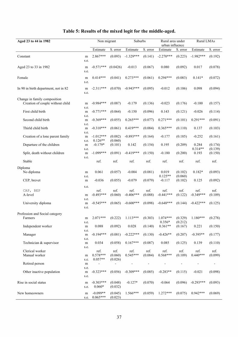
Table 5: Results of the mixed logit for the middle-aged.
Aged 23 to 44 in 1982 Non migrant Suburbs Rural area under
urban influence
Rural LMAs
Estimate S. error Estimate S. error Estimate S. error Estimate S. error
Constant m 2.867*** (0.093) -1.329*** (0.141) -2.270*** (0.223) -1.982*** (0.192)
s.e.
Aged 23 to 33 in 1982 m -0.571*** (0.0426) -0.013 (0.067) 0.080 (0.092) 0.017 (0.078)
s.e.
Female m 0.414*** (0.041) 0.273*** (0.061) 0.294*** (0.083) 0.141* (0.072)
s.e.
In 90 in birth department, not in 82 m -2.311*** (0.070) -0.943*** (0.095) -0.012 (0.106) 0.098 (0.094)
s.e.
Change in family composition
Creation of couple without child m -0.984*** (0.087) -0.179 (0.136) -0.023 (0.176) -0.100 (0.157)
s.e.
First child birth m -0.771*** (0.064) -0.150 (0.096) 0.143 (0.121) -0.026 (0.114)
s.e.
Second child birth m -0.369*** (0.055) 0.265*** (0.077) 0.271*** (0.101) 0.291*** (0.091)
s.e.
Thirld child birth m -0.310*** (0.061) 0.419*** (0.084) 0.365*** (0.110) 0.137 (0.103)
s.e.
Creation of a lone parent family m -1.012*** (0.082) -0.893*** (0.164) -0.177 (0.185) -0.252 (0.161)
s.e. 0.126** (0.060)
Departure of the children m -0.179* (0.101) 0.142 (0.154) 0.195 (0.209) 0.284 (0.174)
s.e. 0.314** (0.139)
Split, death without children m -1.099*** (0.091) -0.419*** (0.150) -0.180 (0.200) 0.193 (0.150)
s.e.
Stable ref. ref. ref. ref. ref. ref. ref. ref.
Diploma
No diploma m 0.061 (0.057) -0.004 (0.081) 0.019 (0.102) 0.182* (0.093) s.e. 0.125** (0.060)
CEP, brevet m -0.036 (0.055) -0.079 (0.079) -0.117 (0.102) 0.125 (0.092)
s.e. CAP, BEP ref. ref. ref. ref. ref. ref. ref. ref.
A-level m -0.493*** (0.060) -0.406*** (0.088) -0.441*** (0.122) -0.349*** (0.109)
s.e.
University diploma m -0.545*** (0.065) -0.600*** (0.098) -0.648*** (0.144) -0.422*** (0.125)
s.e.
Profession and Social category
Farmers m 2.071*** (0.222) 1.113*** (0.303) 1.074*** (0.329) 1.180*** (0.278)
s.e. 0.356* (0.212)
Independent worker m 0.088 (0.092) 0.028 (0.140) 0.361** (0.167) 0.221 (0.150)
s.e.
Manager m -0.194*** (0.081) -0.222*** (0.130) -0.426** (0.207) -0.395** (0.177)
s.e.
Technician & supervisor m 0.034 (0.058) 0.167*** (0.087) 0.085 (0.125) 0.139 (0.110)
s.e.
Clerical worker ref. ref. ref. ref. ref. ref. ref. ref.
Manual worker m 0.578*** (0.060) 0.545*** (0.084) 0.568*** (0.109) 0.440*** (0.099)
s.e. 0.057** (0.026)
Retired person m - - - - - - - -
s.e.
Other inactive population m -0.323*** (0.056) -0.309*** (0.085) -0.283** (0.115) -0.021 (0.098)
s.e.
Rise in social status m -0.303*** (0.048) -0.127* (0.070) -0.064 (0.096) -0.293*** (0.093)
s.e. 0.060* (0.032)
New homeowners m -0.099** (0.045) 1.566*** (0.059) 1.272*** (0.075) 0.942*** (0.069)
s.e. 0.065*** (0.023)
37

Table 5 (continued)
Aged 23 to 44 in 1982 Non migrant Suburbs Rural area under
urban influence
Rural LMAs
Estimate S. error Estimate S. error Estimate S. error Estimate S. error
Population density and LMA size in 1982
In a rural LMA in 1982 m -0.611*** (0.078) -0.336*** (0.118) 0.728*** (0.190) 1.186*** (0.159)
s.e. 0.106** (0.052)
low density and small urban LMA m -0.405*** (0.079) 0.489*** (0.114) 0.538*** (0.194) 0.184 (0.169)
s.e.
low density and big urban LMA m -0.484*** (0.080) 0.300*** (0.120) -0.162 (0.212) -0.630*** (0.203)
s.e.
medium density and small urban LMA m -0.409*** (0.083) 0.663*** (0.119) 0.318 (0.204) 0.145 (0.177)
s.e.
medium density and big urban LMA m -0.022 (0.072) 0.438*** (0.106) 0.043 (0.190) 0.054 (0.156)
s.e. 0.087* (0.045)
high density ref. ref. ref. ref. ref. ref. ref. ref.
Ile de France in 1982 m 0.392*** (0.064) 0.437*** (0.090) -0.166 (0.166) -0.068 (0.139)
s.e.
Unemp. rate ≤ 8% in 1982 location m 0.102*** (0.039) 0.087 (0.058) 0.062 (0.074) 0.249*** (0.066)
s.e. 0.055* (0.033) 0.081** (0.042)
Log likelihood = -28,529
Observations = 37,299
*** : coefficient significant at the 1% level ; ** : at the 5% level ; * : at the 10% level.
- : variable not relevant for this age range
38

Table 6: Results of the mixed logit for the oldest
Aged 45 to 64 in 1982 Non migrant Suburbs Rural area under
urban influence
Rural LMAs
Estimate S. error Estimate S. error Estimate S. error Estimate S. error
Constant m 3.845*** (0.186) -0.585** (0.284) -0.646** (0.300) -0.830*** (0.284)
s.e.
Female m -0.036 (0.080) -0.015 (0.129) -0.142 (0.130) -0.014 (0.115)
s.e.
In 90 in birth department, not in 82 m -4.298*** (0.162) -0.682*** (0.156) -0.326** (0.147) 0.042 (0.126)
s.e.
Change in family composition
Creation of couple without child m -0.483*** (0.169) -0.298 (0.302) 0.010 (0.291) -0.227 (0.255)
s.e. 0.295*** (0.103) 0.563*** (0.216)
First child birth m 0.238 (0.241) 0.371 (0.339) -0.615 (0.457) -0.199 (0.369)
s.e.
Second child birth m 0.391 (0.536) 0.071 (0.774) -0.032 (0.777) -0.273 (0.947)
s.e.
Thirld child birth m -0.477 (0.491) -0.295 (0.806) -0.443 (0.976) -0.125 (0.705)
s.e.
Creation of a lone parent family m -0.587*** (0.186) -0.449 (0.324) -1.442*** (0.507) -1.240*** (0.435)
s.e.
Departure of the children m 0.097 (0.097) 0.266* (0.143) 0.321** (0.143) 0.309** (0.132)
s.e. 0.095* (0.053)
Split, death without children m -0.943*** (0.101) -0.611*** (0.188) -0.624*** (0.199) -0.165 (0.153)
s.e.
Stable ref. ref. ref. ref. ref. ref. ref. ref.
Diploma
No diploma m 0.150 (0.117) 0.111 (0.178) -0.069 (0.186) 0.311* (0.175)
s.e.
CEP, brevet m 0.088 (0.116) 0.031 (0.178) 0.061 (0.181) 0.055 (0.175)
s.e.
CAP, BEP ref. ref. ref. ref. ref. ref. ref. ref.
A-level m -0.385*** (0.143) -0.358 (0.235) -0.657** (0.262) -0.320 (0.229)
s.e.
University diploma m -0.323** (0.154) -0.656** (0.267) -0.724** (0.287) -0.416 (0.262)
s.e.
Profession and Social category
Farmers m 1.230*** (0.249) 0.345 (0.378) 0.567* (0.343) 0.860*** (0.297)
s.e.
Independent worker m -0.227 (0.149) 0.125 (0.220) -0.146 (0.241) -0.539** (0.227)
s.e.
Manager m -0.664*** (0.156) -0.361 (0.252) -0.397 (0.274) -0.902*** (0.262)
s.e. 0.460*** (0.149)
Technician & supervisor m -0.242* (0.131) -0.083 (0.207) 0.040 (0.215) 0.022 (0.190)
s.e.
Clerical worker ref. ref. ref. ref. ref. ref. ref. ref.
Manual worker m 0.532*** (0.146) 0.393* (0.209) 0.450** (0.211) 0.360* (0.194)
s.e.
Retired person m -0.233* (0.129) -0.432** (0.219) -0.580** (0.229) -0.263 (0.189)
s.e. 0.265* (0.154)
Other inactive population m -0.217* (0.113) -0.307* (0.174) -0.152 (0.183) -0.375** (0.162)
s.e.
Rise in social status m -0.192 (0.182) -0.332 (0.307) -1.167*** (0.451) -0.611* (0.323)
s.e. 0.751** (0.366)
New homeowners m -1.496*** (0.084) 0.883*** (0.114) 0.802*** (0.120) 0.829*** (0.107)
s.e.
39

Table 6 (continued)
Aged 45 to 64 in 1982 Non migrant Suburbs Rural area under
urban influence
Rural LMAs
Estimate S. error Estimate S. error Estimate S. error Estimate S. error
Population density and LMA size in 1982
In a rural LMA in 1982 m -0.356*** (0.138) -0.587*** (0.215) 0.282 (0.231) 0.715*** (0.208)
s.e.
low density and small urban LMA m -0.279* (0.144) 0.069 (0.220) -0.124 (0.249) 0.023 (0.224)
s.e.
low density and big urban LMA m -0.236 (0.151) 0.339 (0.225) -0.275 (0.269) -0.329 (0.253)
s.e.
medium density and small urban LMA m -0.159 (0.159) 0.123 (0.235) -0.229 (0.276) -0.024 (0.246)
s.e.
medium density and big urban LMA m -0.216* (0.126) 0.024 (0.191) 0.078 (0.204) -0.141 (0.190)
s.e.
high density ref. ref. ref. ref. ref. ref. ref. ref.
Ile de France in 1982 m -0.099 (0.114) 0.197 (0.167) 0.370* (0.191) 0.421** (0.172)
s.e. 0.177* (0.095) 0.176** (0.085)
Unemp. rate ≤ 8% in 1982 location m 0.011 (0.074) 0.045 (0.116) -0.049 (0.119) 0.163 (0.104)
s.e. 0.111* (0.068)
Log likelihood = -11,383
Observations = 25,476
*** : coefficient significant at the 1% level ; ** : at the 5% level ; * : at the 10% level.
40

Table 7: Estimation of the probability to choose each destination against urban
destination. The impact of the crossed variable: educational level*origin area
(As the estimation is stable, only the results of the crossed-variable are reported)
Non migrant Suburbs Rural area under
urban influence
Rural LMAs
Estimate S. error Estimate S. error Estimate S. error Estimate S. error
Aged 15 to 22 in 1982
Univ. diploma x urban LMA m ref. ref. ref. ref. ref. ref. ref. ref.
Univ. diploma x rural LMA m -0.185 0.167 -0.400 0.278 0.212 0.373 1.332*** 0.373
s.e.
Educ. level under univ.x urban LMA m 0.593*** 0.067 0.490*** 0.125 0.179 0.186 0.185 0.159
s.e.
Educ. level under univ.x rural LMA m 0.725*** 0.131 -0.298 0.209 0.948*** 0.299 2.289*** 0.342
s.e.
Aged 23 to 44 in 1982
Univ. diploma x urban LMA m ref. ref. ref. ref. ref. ref. ref. ref.
Univ. diploma x rural LMA m 0.027 0.152 -0.040 0.227 0.969*** 0.294 1.559*** 0.289
s.e.
Educ. level under univ.x urban LMA m 0.342*** 0.057 0.513*** 0.088 0.524*** 0.140 0.299** 0.126
s.e.
Educ. level under univ.x rural LMA m 0.500*** 0.119 -0.497*** 0.176 1.192*** 0.247 1.969*** 0.260
s.e.
Aged 45 to 64 in 1982
Univ. diploma x urban LMA m ref. ref. ref. ref. ref. ref. ref. ref.
Univ. diploma x rural LMA m 0.312 0.394 -1.295 1.289 1.214* 0.623 1.952*** 0.585
s.e. 0.7045** 0.347
Educ. level under univ.x urban LMA m 0.298** 0.131 0.675*** 0.236 0.644** 0.259 0.635** 0.255
s.e.
Educ. level under univ.x rural LMA m 0.444* 0.230 -0.642* 0.374 1.206*** 0.422 1.855*** 0.414
s.e. 0.164** 0.084
*** : coefficient significant at the 1% level ; ** : at the 5% level ; * : at the 10% level.
41


