Download - Lecture on Radio Propagatio

ETE 424/EEE 424Mobile and Wireless Communications
Dr. Arshad M. ChowdhuryAssociate ProfessorDept. of Electrical and Computer EngineeringNorth South University
Chapter 4 – Mobile Radio Propagation: Large-Scale Path Loss

Non Line of Sight (NLOS)
• Three basic propagation mechanisms in addition to line-of-sight paths– Reflection - Waves bouncing off of objects of large
dimensions – Diffraction - Waves bending around sharp edges of
objects – Scattering - Waves traveling through a medium with
small objects in it (foliage, street signs, lamp posts, etc.) or reflecting off rough surfaces

Reflections• Reflection occurs when RF energy is incident upon a boundary between two
materials (e.g. air/ground) with different electrical characteristics– Example: reflections from earth and buildings
• These reflections may interfere with the original signal constructively or destructively
• Upon reflection or transmission, a ray attenuates by factors that depend on the frequency, the angle of incidence, and the nature of the medium (its material properties, thickness homogeneity, etc.)
• The amount of reflection depends on the reflecting material.– Smooth metal surfaces of good electrical conductivity are efficient reflectors of radio waves.– The surface of the Earth itself is a fairly good reflector.
• Fresnel reflection coefficient → Γ – describes the magnitude of reflected RF energy – depends upon material properties, polarization, & angle of incidence

Ground Reflection (2-Ray) Model• In a mobile radio channel, a single direct path between the
base station and mobile is rarely the only physical path for propagation
• Free space propagation model in most cases is inaccurate when used alone
• 2 Ray Ground Reflection Model: considers both- direct path and ground reflected propagation path between transmitter and receiver• Reasonably accurate for predicting large scale signal strength over
distances of several kilometers for mobile radio systems using tall towers (above 50 m )

Ground Reflection (2-Ray) Model
• The maximum T-R separation distance ( In most mobile systems ) is only a few tens of kms, and the earth may be assumed to be flat.
• ETOT is the electric field that results from a combination of a direct line-of-sight path and a ground reflected path
ETOT = ELOS + Eg

is the amplitude of the electric field at distance d
6
ETOT is the electric field that results from a combination of a direct line-of-sight path and a ground reflected path
ωc = 2πfc where fc is the carrier frequency of the signal
At different distances d the wave is at a different phase

Method of imageThe method of images is used to find the path difference between the line-of-sight and the ground reflected paths
ht : Transmitter height, hr : Receiver heightd: horizontal distance between T-Rd’: Line of sight path distance between T-Rd” : ground reflected path distance between T-R
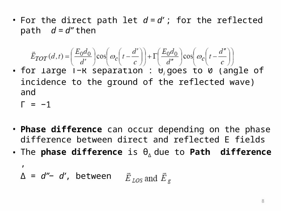
• For the direct path let d = d’ ; for the reflected path d = d” then
• for large T−R separation : θi goes to 0 (angle of incidence to the ground of the reflected wave) and Γ = −1
• Phase difference can occur depending on the phase difference between direct and reflected E fields
• The phase difference is θ∆ due to Path difference ,
∆ = d”− d’, between
8
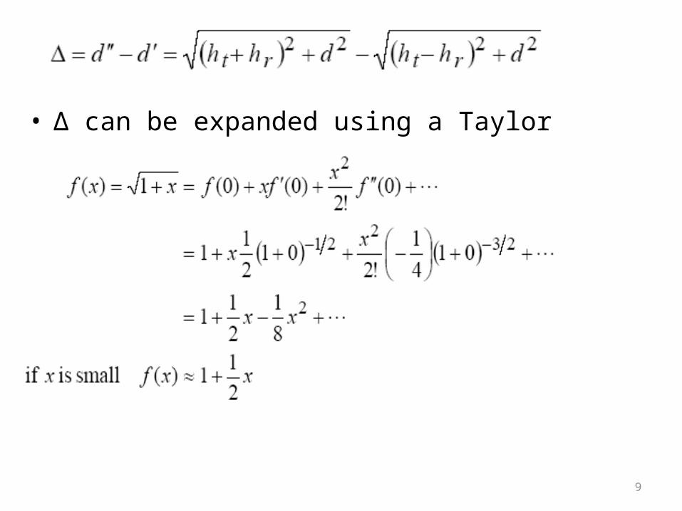
• ∆ can be expanded using a Taylor series expansion
9
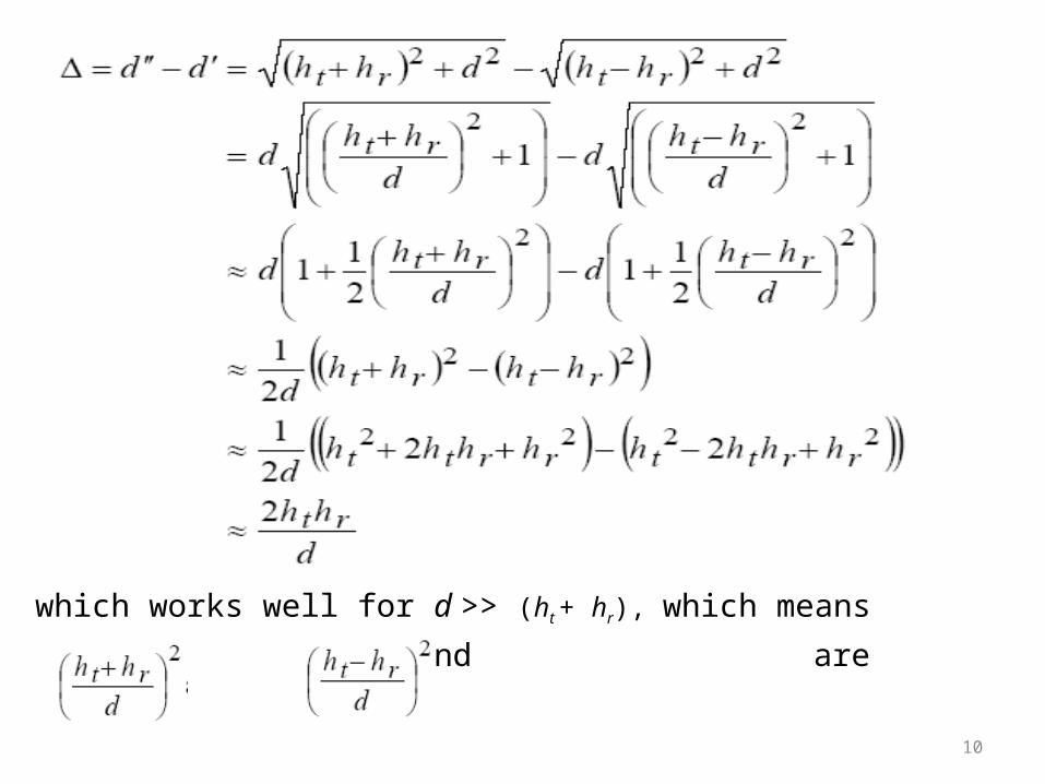
which works well for d >> (ht + hr), which means and are small
10
11
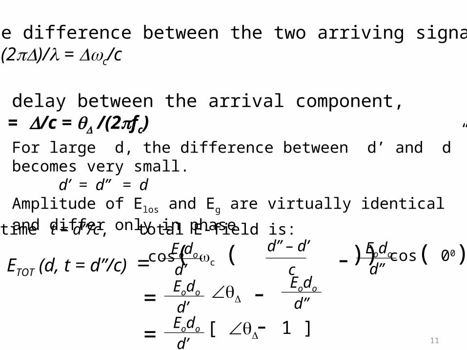
The phase difference between the two arriving signals is = (2)/ = c/c
The time delay between the arrival component, d = /c = /(2fc)
For large d, the difference between d’ and d” becomes very small. d’ = d” = d
Amplitude of Elos and Eg are virtually identical and differ only in phase
ETOT (d, t = d”/c) =
Eodo
d’cos( c ( )) d” – d’
cEodo
d”cos( 00) -
At time t = d”/c, total E-field is:
Eodo
d’Eodo
d” -=
Eodo
d’[ - 1 ]=
12
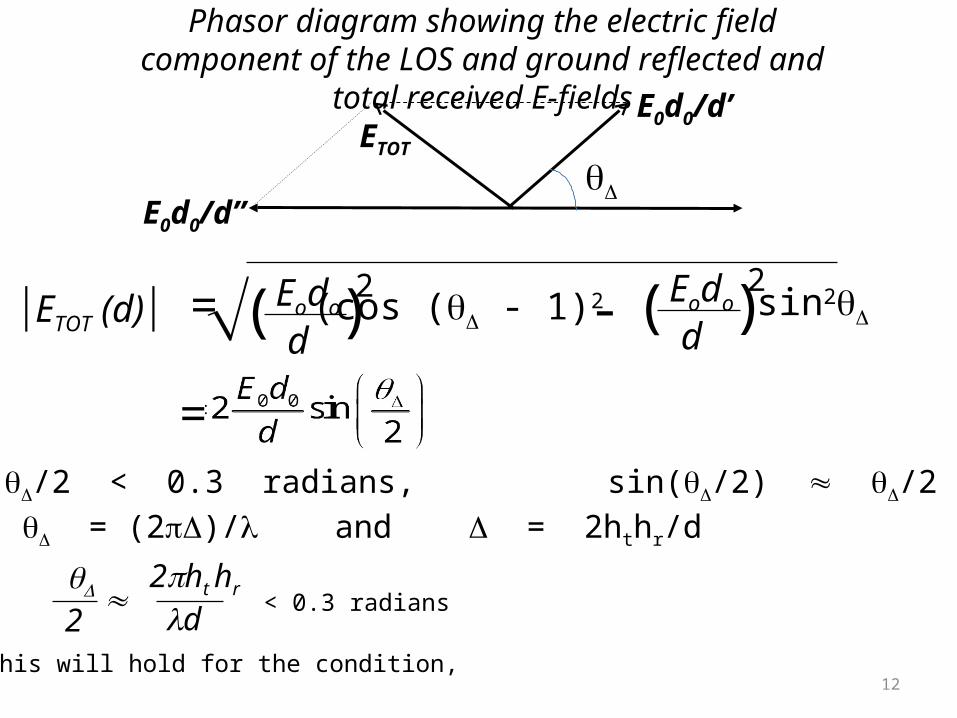
Phasor diagram showing the electric field component of the LOS and ground reflected and total received E-fields
E0d0/d’
E0d0/d”
ETOT
ETOT (d) =
-(cos ( - 1)2 Eodo
d( )2 Eodo
dsin2( )2
=
For /2 < 0.3 radians, sin(/2) /2 Again, = (2)/ and = 2hthr/d
2ht hr
d
2< 0.3 radians
This will hold for the condition,
13
ETOT(d) 2 Eodo
d2hthr
d kd2
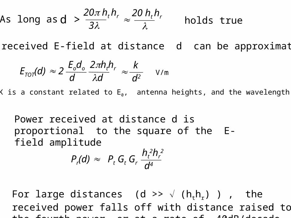
d > 20 ht hr
3 20 ht hr
As long as holds true
The total received E-field at distance d can be approximated as:
V/m
K is a constant related to E0, antenna heights, and the wavelength
Power received at distance d is proportional to the square of the E-field amplitude
Pr(d) Pt Gt Gr ht
2hr2
d4
For large distances (d >> (hthr) ) , the received power falls off with distance raised to the fourth power, or at a rate of 40dB/decade
14
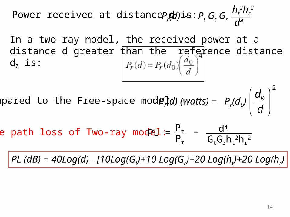
Pr(d) Pt Gt Gr ht
2hr2
d4
The path loss of Two-ray model: PtPr
= d4
GtGrht2hr
2PL =
PL (dB) = 40Log(d) - [10Log(Gt)+10 Log(Gr)+20 Log(ht)+20 Log(hr)
In a two-ray model, the received power at a distance d greater than the reference distance d0 is:
Compared to the Free-space model:
Power received at distance d is:
Pr(d) (watts) = Pr(d0)2
0
dd
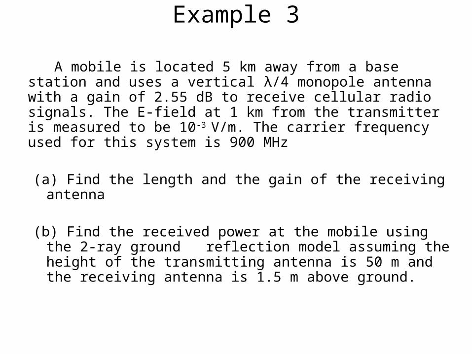
Example 3
A mobile is located 5 km away from a base station and uses a vertical λ/4 monopole antenna with a gain of 2.55 dB to receive cellular radio signals. The E-field at 1 km from the transmitter is measured to be 10-3 V/m. The carrier frequency used for this system is 900 MHz
(a) Find the length and the gain of the receiving antenna
(b) Find the received power at the mobile using the 2-ray ground reflection model assuming the height of the transmitting antenna is 50 m and the receiving antenna is 1.5 m above ground.

Given:T-R separtion distance, d = 5 kmReference distance d0 = 1km
E-field at d0 = 10-3 V/m
Operating frequency, f = 900 MHzwavelength, = c/f = (3x10⁸)/ (900x106) = 0.333 m
a) The length of the monopole antenna = /4 = 0.333/4 = 0.0833m = 8.33cm
The antenna gain, G is related to the effective aperture, Ae :
G = (4 Ae)/ 2
Gain, G = 2.55 dB = 1.8 and wavelength, = 0.333mEffective Aperture Area, Ae = 1.8 x (0.333)2 / 4 = 0.016 m2

b) Height of transmitter antenna, ht = 50m
Height of receiver antenna, hr = 1.5 m
T-R distance, d = 5 km(hthr) = (50x1.5) = 8.66 m
since, d >> (hthr), the E-field at distance d = 5 km is:
ETOT(d) 2 Eodo
d2hthr
d kd2 V/m
ETOT(d) = 2 x (10-3)x (1x103)
(5x10³) [ ]2x 3.14x 50x 1.5 (0.333)x(5x103)
ETOT(d) = 113.1x10⁻⁶ v/m
The received power at distance, d is given by:
Pr(d) = Pd(d). Ae = ETOT2
120 . Ae =
( 113.1x10⁻⁶)2 x 0.016120
= 5.4 x 10⁻¹³ W = -122.68 dBW = -92 dBm

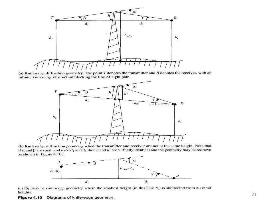
Diffraction• Occurs when the radio path between sender and receiver is obstructed
by an impenetrable body and by a surface with sharp irregularities (edges)
• The received field strength decreases rapidly as a receiver moves deeper into the obstructed (shadowed) region, the diffraction field still exists and often has sufficient strength to produce a useful signal.
• Diffraction explains how radio signals can travel urban and rural environments without a line-of-sight path

Diffraction• Phenomenon of diffraction can be explained by Huygen's principle
– All points on a wave front can be considered as point sources for the production of secondary wavelets
– these 'wavelets combine to produce a new wave front in the direction of propagation
– The field strength of a diffracted wave in the shadowed region is the vector sum of the electric field components of all the secondary wavelets in the space around the obstacle.

• excess path length : The difference between the direct path and diffracted path
• Fresnel-Kirchoff diffraction parameter
• The corresponding phase difference
20
• The diffraction gain due to the presence of a knife edge, as compared the the free space E-field
E0 : Electric field in free spaceEd: Electric field in the presence of Knife-edge
21

Scattering• The medium which the wave travels consists of objects with dimensions
smaller than the wavelength and where the number of obstacles per unit volume is large – rough surfaces, small objects, foliage, street signs, lamp posts.
• Received signal strength is often stronger than that predicted by reflection/diffraction models alone
22
The EM wave incident upon a rough or complex surface is scattered in many directions and provides more energy at a receiver energy that would have been absorbed is instead reflected to the Rx.flat surface → EM reflection (one direction)rough surface → EM scattering (many directions)

Propagation Models• Large scale models predict behavior averaged over
distances much larger than wavelength – Function of distance & significant environmental
features, roughly frequency independent– Breaks down as distance decreases– Useful for modeling the range of a radio system and
rough capacity planning• To predict large scale coverage using analytical and
empirical (field data) methods are used• Various path loss models for indoor/outdoor wireless
communications
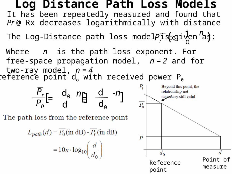
Log Distance Path Loss Models
The Log-Distance path loss model is given as: Pr ( )1d
n
Where n is the path loss exponent. For free-space propagation model, n = 2 and for two-ray model, n = 4
At a reference point do with received power P0
Pr
P0[ ]d0
dn [ ]d
d0
-n= =
Reference point
Point of measure
It has been repeatedly measured and found that Pr @ Rx decreases logarithmically with distance

Typical large-scale path loss

26
• Log Distance Path loss does not consider the surrounding environmental impacts
• Shadowing occurs when objects block LOS between TX and RX• A simple statistical model can account for unpredictable “shadowing” • Log-Normal Shadowing:
PL (d) = PL (do ) + 10 n log (d / do ) + Xσ
– describes how the path loss at any specific location may vary from the average value
– Includes the large-scale path loss component plus a random amount Xσ.
• Xσ : zero mean Gaussian random variable• σ is the standard deviation that provides the second parameter for the
distribution• n & σ are computed from measured data for different area types
Log-Normal Shadowing Model

27
Measured large-scale path loss
Check Example 4.9

Okumura Model• It is one of the most widely used models for signal prediction in
urban areas, and it is applicable for frequencies in the range 150 MHz to 1920 MHz
• Based totally on measurements (not analytical calculations)• Applicable in the range: 150MHz to ~ 2000MHz, 1km to 100km
T-R separation, Antenna heights of 30m to 100m
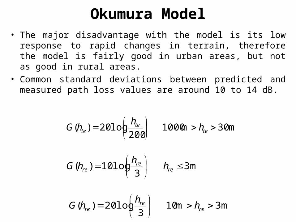
Okumura Model• The major disadvantage with the model is its low response to rapid
changes in terrain, therefore the model is fairly good in urban areas, but not as good in rural areas.
• Common standard deviations between predicted and measured path loss values are around 10 to 14 dB.
m30m1000200
log20)(
te
tete hhhG
m33
log10)(
re
rere hhhG
m3m103
log20)(
re
rere hhhG

Median Attenuation and Correction Factors
Please see Example 4:10 to understand the usage of these charts
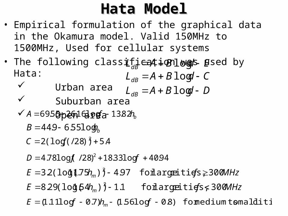
Hata ModelHata Model• Empirical formulation of the graphical data in the Okamura model.
Valid 150MHz to 1500MHz, Used for cellular systems• The following classification was used by Hata:
Urban area Suburban area Open area
EdBALdB logCdBALdB logDdBALdB log
bhfA 82.13log16.2655.69
bhB log55.69.44
94.40log33.18)28/log(78.4 2 ffD
4.5))28/(log(2 2 fC
MHzfhE m 300 cities, largefor 97.4))75.11(log(2.3 2
MHzfhE m 300 cities, largefor 1.1))54.1(log(29.8 2
cities small tomediumfor )8.0log56.1()7.0log11.1( fhfE m
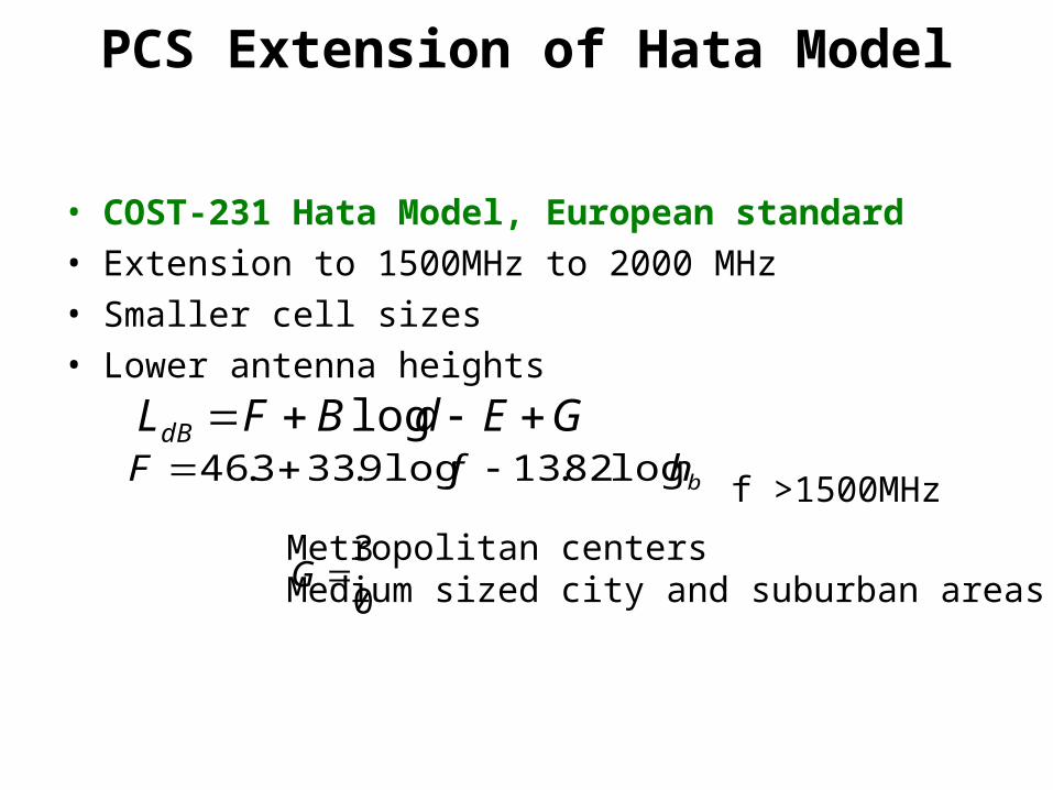
PCS Extension of Hata Model
• COST-231 Hata Model, European standard• Extension to 1500MHz to 2000 MHz • Smaller cell sizes• Lower antenna heights
GEdBFLdB logbhfF log82.13log9.333.46 f >1500MHz
03
GMetropolitan centersMedium sized city and suburban areas


